


Highlights
What are the main findings?
- CA-Mamba achieves competitive binary change detection performance across four public benchmarks, reaching an F1-score of 80.45% on CLCD.
- On LEVIR-CD and CLCD, the full model achieves slightly higher F1-score and IoU than variants without explicit signed-difference pathways or with parameter-matched plain convolutional heads.
What are the implications of the main findings?
- Bi-temporal differences can guide state-space parameter generation and boundary-aware decoding, extending their role beyond feature fusion.
- Practical use of CA-Mamba requires balancing detection accuracy against parameter storage and measured inference latency, rather than judging efficiency from FLOPs alone.
Abstract
Remote sensing binary change detection aims to identify real changes in bi-temporal images while suppressing pseudo-change responses induced by complex backgrounds and temporal variations in otherwise unchanged regions. Although existing state-space-based methods incorporate cross-temporal interaction, integrating explicit difference priors into state-space parameter generation and subsequent boundary-aware decoding remains an important design problem. To address this problem, CA-Mamba, a change-aware Mamba decoding framework, is proposed. An Asymmetric Change-Aware State-Space Mixer (ACSSM) is introduced to condition state-space parameter generation on bi-temporal difference priors and to modulate the two temporal branches asymmetrically. The Cascaded Difference Prior Module (CDPM), the Change Boundary Enhancement (CBE) module, and the Change Representation Constructor (CRC) are further integrated into a unified pipeline for difference-prior generation and propagation, change-aware mixing, boundary enhancement, and region–boundary collaborative representation construction. Experiments on four public datasets, namely, LEVIR-CD, WHU-CD, CDD, and CLCD, show competitive detection performance. Ablation results support the use of signed-difference pathways and the overall CRC design under the evaluated settings. The efficiency analysis characterizes the trade-offs among detection accuracy, reported computational cost, inference latency, and parameter storage.
1. Introduction
Remote sensing change detection is used to identify changes in surface objects, land-cover patterns, and scene structures from multi-temporal imagery, and it has been widely applied to urban expansion monitoring, land-use change analysis, disaster assessment, and resource investigation [1,2,3,4]. As a common setting in this field, binary change detection (BCD) aims to distinguish changed regions from unchanged ones. In practice, however, BCD remains challenging. Bi-temporal images are often affected by illumination variation, seasonal effects, sensor-induced appearance differences, and registration errors, which may produce pseudo-change responses unrelated to true surface changes [3,5,6]. In addition, real changes usually occupy only a small part of the scene, whereas large unchanged background regions dominate the feature distribution and may interfere with cross-temporal interaction [5,6,7,8,9]. Therefore, effective BCD requires reliable semantic discrimination, strong pseudo-change suppression, and precise boundary localization [8,10,11].
Early remote sensing change detection methods mainly relied on image differencing, change vector analysis, image transformation analysis, and conventional machine learning techniques [1,2]. In these methods, change inference was typically performed from handcrafted descriptors or pixel-level statistical differences. For synthetic aperture radar (SAR) change detection, Li et al. [12] use principal component analysis to fuse difference images before two-level clustering. Although such methods were effective in some scenarios, their representation capacity and scene adaptability were limited, making them less suitable for complex backgrounds, imaging disturbances, and fine-grained structural variations in high-resolution imagery [1,2,3]. With the rapid development of deep learning, CNN-based Siamese networks, fully convolutional networks, and encoder–decoder architectures were adopted as mainstream solutions for change detection. By learning discriminative local patterns from bi-temporal images, these methods substantially improved detection performance [13,14]. Multi-scale fusion, attention mechanisms, feature constraints, and cross-temporal interaction strategies were further introduced to enhance change-region representation [9,14,15,16,17,18,19]. Nevertheless, CNNs are still constrained by local convolution operations. Long-range dependencies and cross-region semantic relationships are therefore difficult to model effectively, and local details may be weakened during multi-scale propagation.
To overcome the limited global modeling capability of CNNs, Transformer-based methods have been introduced into remote sensing change detection. Through self-attention, long-range dependencies can be established across distant spatial positions, and contextual perception as well as cross-temporal semantic interaction can be strengthened in complex scenes [10,20,21,22]. Subsequent studies further explored cross-temporal difference modeling, global context aggregation, bi-temporal feature alignment, and structure-preserving decoding to improve the discrimination of real changes from spurious responses [5,6,7,8,10,11,23,24]. However, due to the quadratic complexity of self-attention, high computational and memory costs are usually incurred. This limits the efficiency of Transformers in high-resolution remote sensing imagery and dense prediction tasks [20,21]. Therefore, a better balance among global modeling capability, local boundary recovery, and computational efficiency is still needed.
Recently, state-space models (SSMs), exemplified by Mamba, have emerged as a promising alternative for efficient long-range dependency modeling because state propagation is input-adaptive, and the computational complexity is approximately linear with respect to sequence length [25]. With the development of visual state-space architectures such as Vision Mamba, VMamba, and LocalMamba [26,27,28], encouraging results have also been reported in remote sensing dense prediction and change detection tasks [29,30,31,32,33,34,35,36]. Existing designs explore spatial scanning, local–global representation learning, and cross-temporal interaction; CDMamba, for example, uses information from one temporal image to guide the features of the other [32]. These developments motivate a more specific question: how can explicit bi-temporal difference priors condition state-space parameter generation and remain available for boundary refinement and prediction construction throughout decoding? CA-Mamba addresses this question through cascaded difference-conditioned decoding, rather than treating cross-temporal interaction itself as a new capability.
Accordingly, a change-aware Mamba decoding framework for remote sensing binary change detection, termed CA-Mamba, is proposed. In CA-Mamba, difference priors are introduced during decoding to steer state-space propagation toward change-oriented bi-temporal feature interaction. The Cascaded Difference Prior Module (CDPM) first generates and propagates stable multi-scale difference priors. Guided by these priors, the Asymmetric Change-Aware State-Space Mixer (ACSSM) performs change-aware state-space mixing with asymmetric modulation from bi-temporal differences. The Change Boundary Enhancement (CBE) module and the Change Representation Constructor (CRC) are then used to refine change boundaries and construct a region–boundary collaborative representation. Finally, the Prediction Refinement Head produces the high-resolution prediction by combining the constructed change representation with a change-intensity map.
Compared with existing methods, the main contributions of this paper are summarized as follows:
- CA-Mamba, a change-aware Mamba decoding framework for remote sensing binary change detection, is proposed. Cascaded bi-temporal difference priors condition state-space parameter generation and are subsequently reused for boundary enhancement and prediction-representation construction. The contribution concerns the source, point of application, and continued use of change guidance within the decoder.
- An Asymmetric Change-Aware State-Space Mixer (ACSSM) is introduced. By incorporating difference priors and asymmetric change modulation into state propagation, feature interaction is shifted from generic content aggregation toward change-driven bi-temporal modeling. This design highlights real changes, suppresses background-induced spurious responses, and improves cross-temporal feature interaction and change discrimination.
- A collaborative modeling mechanism between the Change Boundary Enhancement (CBE) module and the Change Representation Constructor (CRC) is developed. CBE enhances change-related boundary responses while suppressing spurious boundary interference. CRC further constructs a prediction-oriented representation that jointly encodes change regions and structural boundaries, thereby improving response continuity, region completeness, and structural consistency through cross-scale propagation.
The remainder of this paper is organized as follows. Section 2 reviews related work. Section 3 presents the materials and methods, including the proposed CA-Mamba framework, datasets, experimental settings, evaluation metrics, and compared methods. Section 4 reports the comparative experiments, ablation studies, and visual analyses. Section 5 discusses the findings, practical implications, and limitations. Section 6 concludes this paper.
2. Related Work
This section reviews three categories of methods related to CA-Mamba: CNN-based, Transformer-based, and Mamba/SSM-based change detection methods. The discussion focuses on local detail representation, global context modeling, cross-temporal interaction, and efficient long-range dependency modeling.
2.1. CNN-Based Change Detection Methods
With the development of deep learning, CNN-based methods have been widely adopted for remote sensing change detection. Early representative studies used fully convolutional Siamese networks to extract bi-temporal features and perform change discrimination through feature concatenation or differencing [13,14]. Compared with traditional handcrafted methods, more discriminative local and semantic representations can be learned by CNN-based models, leading to clear improvements in complex remote sensing scenes.
Subsequent studies further improved CNN-based change detection through multi-scale fusion, deep supervision, attention mechanisms, dense connections, feature constraints, and cross-temporal interaction [9,14,15,16,17,18,19]. For example, DSIFN enhanced the fusion of deep bi-temporal features and difference features through deep supervision [17]. STANet introduced spatial-temporal attention to alleviate the influence of registration errors and pseudo-change responses [18]. SNUNet-CD strengthened multi-level information propagation with a densely connected Siamese structure [19], while HANet improved multi-scale representation through hierarchical attention [9]. FCCDN and Changer further enhanced change discrimination from the perspectives of feature constraints and feature interaction, respectively [15,16].
Although CNN-based methods are effective in local texture modeling, boundary detail recovery, and hierarchical feature representation, their global modeling ability is still limited by local convolution operations. When change regions are sparse, background structures are complex, or large unchanged areas dominate the scene, long-range semantic relationships may be insufficiently captured. In addition, local change cues can be weakened during multi-scale feature propagation. Therefore, it remains important to enhance global feature interaction while preserving local details and boundary structures.
2.2. Transformer-Based Change Detection Methods
Transformer-based methods have been introduced into remote sensing change detection to strengthen global context modeling. By using self-attention, long-range dependencies can be established across distant spatial positions, which helps improve contextual perception and cross-temporal semantic interaction. BIT converted bi-temporal features into semantic tokens and modeled global relationships with a Transformer [20]. SwinSUNet introduced the Swin Transformer into a U-shaped architecture to improve multi-scale semantic modeling and change-region recovery [21]. ChangeFormer and TransUNetCD further combined Siamese or dual-branch designs with Transformer encoders or decoders to balance local feature extraction and global context modeling [22,23]. MSCANet also demonstrated the effectiveness of CNN-Transformer hybrid modeling for fine-grained cropland change detection [24].
Further efforts have been made to improve cross-temporal difference modeling, global context perception, feature alignment, and spurious-change suppression. Cross-temporal Difference Transformer emphasized the importance of modeling temporal difference relationships [10]. GCFormer enhanced change discrimination through global context modeling [7]. BiFA addressed bi-temporal feature misalignment by feature alignment [5]. Semantic-explicit Filtering Network suppressed pseudo-change responses through semantic filtering [6]. MaskCD improved structural representation through mask classification, and CSTSUNet progressively injected detail and boundary information during decoding [8,11].
Related remote sensing object detection studies also address detail preservation during multi-scale feature extraction. Song et al. [37] separate shallow detail and semantic processing in DSH-DETR, while Hu et al. [38] use two-stage frequency-domain enhancement in TSF-DETR to strengthen small-object features. These studies concern object localization rather than bi-temporal change discrimination; their relevance here is the preservation of fine details during feature propagation.
Despite their strong global modeling capability, Transformer-based methods usually require high computational and memory costs because of the quadratic complexity of self-attention [20,21]. Window-based attention, hierarchical designs, and CNN-Transformer hybrid frameworks can reduce this burden to some extent [21,23,24]. However, trade-offs among global receptive field, local boundary recovery, and inference efficiency still remain, especially for high-resolution dense prediction tasks.
2.3. Mamba/SSM-Based Change Detection Methods
State-space models (SSMs), exemplified by Mamba, provide an efficient alternative for long-range dependency modeling with approximately linear complexity in sequence length [25]. With the development of visual state-space architectures such as Vision Mamba, VMamba, and LocalMamba [26,27,28], Mamba/SSM-based modeling has shown strong potential in visual representation learning and remote sensing dense prediction [33].
Recently, Mamba/SSM-based methods have also been explored for remote sensing change detection. ChangeMamba introduced spatiotemporal state-space modeling to enhance bi-temporal feature interaction [29]. ConMamba, Hybrid-MambaCD, and CWmamba combined CNNs with Mamba/SSM to exploit both local detail representation and long-range dependency modeling [30,31,34]. CDMamba incorporated local cues into Mamba to improve the representation of local details and boundary structures [32]. CD-Lamba and Frequency-Enhanced Mamba further enhanced local change awareness and subtle-change representation through cross-temporal adaptive state propagation and frequency-domain modeling, respectively [35,36].
These studies demonstrate the promise of Mamba/SSM for long-range modeling and cross-temporal interaction in remote sensing change detection. CA-Mamba investigates a complementary decoder design in which explicit difference priors condition state-space parameter generation, asymmetric branch updates, and subsequent boundary-aware representation construction. The architectural differences from RS-Mamba, CDMamba, and LGMM-Net are detailed in Section 3.11.
3. Materials and Methods
This section presents CA-Mamba, a change-aware decoding framework for remote sensing binary change detection. Its central design is to condition state-space parameter generation on explicit bi-temporal difference priors and to reuse these priors during boundary enhancement and cross-scale prediction-representation construction.
To address this problem, CA-Mamba adopts a coarse-to-fine decoding strategy. Stable difference priors are first generated from deep semantic features to steer change-aware state-space mixing. Subsequently, boundary enhancement and region–boundary collaborative representation are progressively introduced to recover fine structures and high-resolution change details. The remainder of this section introduces the preliminaries of state-space modeling, the overall architecture, CDPM, ACSSM, CBE, CRC, the Prediction Refinement Head, and the loss function.
3.1. Preliminaries: State-Space Models
State-space models (SSMs) describe sequential signals by recursively updating hidden states. Given the continuous-time input , hidden state , and output , a standard continuous-time SSM can be written as
where , , and denote the state transition matrix, input mapping matrix, and output mapping matrix, respectively.
After discretization, the hidden-state update and output are formulated as
where denotes the hidden state at position t, and and are the discretized state transition and input mapping matrices.
Mamba further introduces selective state-space modeling, in which parameters such as the discretization step size , , and can be generated or modulated according to the input content [25]. This selective mechanism improves contextual adaptivity while retaining efficient long-range modeling. For visual tasks, a two-dimensional feature map is usually serialized into a sequence of length by spatial flattening or directional scanning. State propagation is then performed on the serialized features, enabling long-range spatial interaction with approximately linear complexity [25,26,27].
For bi-temporal change detection, the conditioning signals supplied to this input-adaptive mechanism are a design choice. CA-Mamba uses explicit difference priors to modulate the inputs generating the state-space parameters, linking the mixing operation to change cues while retaining the two temporal feature streams for subsequent decoding.
3.2. Overall Architecture
Given a bi-temporal input image pair , CA-Mamba first extracts hierarchical features using a shared-weight ConvNeXt-T encoder [39]. The shared encoder keeps the two temporal branches in a consistent representation space. As shown in Figure 1, the network contains four stages indexed by , where denotes the shallowest high-resolution stage, and denotes the deepest semantic stage. The extracted bi-temporal features are formulated as
where denotes the shared encoder, and denotes the number of channels at stage s. The decoder proceeds from to . In this coarse-to-fine process, deep semantic features provide stable difference priors, while shallow features supplement spatial details and boundary cues.
Figure 1.
Overall architecture of CA-Mamba. A shared ConvNeXt-T encoder extracts four-stage bi-temporal features from and . The decoder proceeds from deep to shallow stages, where the Cascaded Difference Prior Module (CDPM), Asymmetric Change-Aware State-Space Mixer (ACSSM), Change Boundary Enhancement (CBE) module, and Change Representation Constructor (CRC) are sequentially applied for difference-prior generation, change-aware mixing, boundary enhancement, and prediction-oriented representation construction. Blue, green, and pink dashed arrows denote cascaded difference-prior propagation, cross-scale prediction propagation, and shallow change-intensity guidance, respectively.
For each decoding stage, CDPM first generates the difference prior . Using this prior, ACSSM performs change-aware state-space mixing and produces and . CBE then enhances change-related boundary responses, yielding and . Finally, CRC constructs the prediction-oriented change representation . This stage-wise pipeline integrates difference-prior generation, change-aware mixing, boundary enhancement, and change representation construction.
Two cross-scale information paths are used in the decoder. The first is the CDPM-driven difference-prior propagation path, which transfers stable difference priors from deep stages to shallow stages. The second is the CRC-driven prediction-representation propagation path, which injects high-level prediction cues into shallow decoding. For stage s, the prediction representation propagated from the deeper stage is aligned as
where denotes spatial upsampling and, when necessary, channel projection. For the deepest stage , this propagation is not performed because no deeper prediction representation exists.
At the final prediction stage, the high-resolution change-intensity map is retained at the shallowest stage to support fine boundary recovery. The final prediction logits are obtained from the shallow prediction representation and through the Prediction Refinement Head, denoted as , where . During inference, the binary change map is obtained by selecting the class with the highest logit at each pixel.
For simplicity, stage superscripts are omitted for some mapping functions in the following subsections. Unless otherwise specified, the corresponding modules share the same structure across stages but use independent parameters. When the channel dimension of a mask differs from that of the modulated feature, channel broadcasting or a projection is used for alignment.
3.3. Cascaded Difference Prior Module (CDPM)
In bi-temporal change detection, change cues have different reliability across feature scales. Shallow features preserve spatial details but are sensitive to texture noise, illumination variation, and registration errors. Deep features provide more stable semantic responses, but their boundary details are relatively coarse. To balance these properties, CDPM is introduced to generate difference priors and propagate them from deep to shallow stages. As illustrated by the blue dashed lines in Figure 1, CDPM consists of current-stage difference-prior generation and cross-scale difference-prior fusion.
For the bi-temporal features at stage s, the current-stage difference prior is generated as
where denotes the signed feature difference, which retains both the magnitude and sign of the difference between the bi-temporal features. The projection mapping compresses the raw difference into a unified feature space. The lightweight wavelet convolution introduces multi-scale structural cues [40], and denotes a polarity-sensitive channel-spatial attention operation. In this way, raw subtraction is transformed into a refined difference prior that is less affected by pseudo changes.
For shallow stages (), the prior from the deeper stage is first aligned to the current resolution and then fused with the current-stage prior through a gated mechanism:
where denotes the deeper prior aligned from stage to stage s. denotes spatial upsampling and, when necessary, a channel projection. The symbol denotes channel-wise concatenation, is the Sigmoid function, and ⊙ denotes element-wise multiplication. For the deepest stage, no deeper prior is available, and is directly set to .
Through this cascaded fusion, shallow noisy differences and deep coarse priors are adaptively balanced. The generated difference priors provide continuous change-oriented guidance for the subsequent ACSSM, CBE, and CRC modules.
3.4. Asymmetric Change-Aware State-Space Mixer (ACSSM)
ACSSM is the core module of CA-Mamba and is designed to perform change-aware global interaction, as illustrated in Figure 2. When state-space mixing is applied to bi-temporal features without explicit change guidance, stable background regions and real change regions may be propagated together. In this case, stable semantics can dominate the state propagation process and weaken the responses to real changes. To address this problem, ACSSM uses the difference prior generated by CDPM as a change condition. Rather than simply concatenating this prior with the input features, ACSSM uses it to guide difference enhancement, branch-specific asymmetric modulation, spatially adaptive state-space mixing, and the final output update.
Figure 2.
Structure of the Asymmetric Change-Aware State-Space Mixer (ACSSM). Blue, green, orange, and purple dashed boxes denote difference enhancement (DE), change-conditioned modulation (CC), asymmetric injection (AI), and spatial masking (SM), respectively. Solid arrows indicate feature flow, including residual and modulation paths. Block and feature-map colors distinguish the labeled operations and tensors; they do not encode numerical values. DE fuses the absolute difference response with the mapped difference prior to form an enhanced change condition. CC and AI generate change-conditioned modulation and branch-specific asymmetric injection, respectively. SM uses the spatial prior-guided mask to modulate the injected tokens before parallel state-space mixing. The change-aware mixed features and are then produced.
The computation of ACSSM consists of one preparatory projection step and four key mechanisms: difference enhancement (DE), change-conditioned modulation (CC), asymmetric injection (AI), and spatial masking (SM). These four mechanisms are later examined through the internal ablation study. In Figure 2, the difference-enhancement branch corresponds to DE, the common change path corresponds to CC, the signed-difference injection with branch-specific addition/subtraction corresponds to AI, and the spatial prior-guided mask before state-space mixing corresponds to SM.
(1) Input Projection and Difference Modeling: Given the bi-temporal features and at stage s, the two temporal branches are first projected into the state-space input domain. Mamba-style output-gating features are also generated. The projected features are then used to construct signed and absolute differences:
where denotes the state-space input representation, and denotes the output-gating feature of temporal branch t. The absolute difference retains the magnitude of the feature difference, whereas the signed difference additionally retains its sign. In CA-Mamba, signed feature differences are used for difference-prior generation and branch-specific feature modulation; their signs do not directly represent semantic change categories such as construction or demolition. Since binary change detection distinguishes only changed and unchanged pixels, no change-direction labels or directional prediction objective are introduced. The practical contribution of the associated processing pathways to binary prediction is evaluated in the additional ablation experiment reported in Section 4.2.
(2) Difference Enhancement (DE): To provide stable change conditions for subsequent state-space mixing, the intra-stage absolute difference is enhanced and combined with the cross-scale difference prior:
where denotes the depthwise difference enhancement operator, denotes the prior mapping, and is a learnable gating parameter. This design preserves local difference responses while introducing semantically stable guidance from CDPM.
(3) Change-Conditioned Modulation and Asymmetric Injection (CC and AI): Shared modulation provides common change context for both temporal branches but does not explicitly introduce branch-specific difference modulation. Therefore, ACSSM decomposes the modulation into a common change component and a signed-difference component:
The shared modulation captures the change context common to both temporal branches, while provides branch-specific modulation based on the signed feature difference. By adding and subtracting the signed term, ACSSM forms distinct injection signals for the two temporal features without changing the binary prediction task.
(4) Spatial Masking and State-Space Mixing (SM): The difference prior is further used to generate a spatial injection mask, which controls where the asymmetric modulation should be strengthened. The masked modulation vectors are then injected into parallel state-space heads:
where is a learnable scaling parameter, denotes the spatial-mask mapping, and is the normalized weight of the k-th state-space head. In our implementation, . The spatial features of each temporal branch are flattened in row-major order, and both heads process the same sequence in the forward direction using separate head-specific parameters. Thus, the two heads do not represent forward and reverse scanning directions. The masked modulation vectors serve as change-conditioned injection signals for the state-space heads, so that selective state propagation is constrained by change cues rather than being driven only by generic content features. In the selective-scan implementation, each injection vector is split into components corresponding to the generated , , and terms, and these components are added to the respective state-space parameter inputs before scanning.
After state-space mixing, the output features are normalized, gated, and refined by a post-mask generated from the difference prior:
where is a learnable scaling parameter, denotes the post-mask mapping, denotes the output projection, and is a learnable residual coefficient. The post-mask term further enhances the output updates in change-related regions indicated by the difference prior. At the implementation level, the residual addition in the last line is performed by the surrounding decoder block after the ACSSM output is returned.
Overall, ACSSM transforms content-driven state-space mixing into change-conditioned bi-temporal interaction. Through DE, stable difference cues are strengthened; through CC and AI, shared change context and branch-specific difference modulation are modeled separately; through SM, state propagation is spatially guided by the difference prior. As a result, more discriminative bi-temporal features are obtained for subsequent boundary enhancement and change representation construction.
3.5. Change Boundary Enhancement and Change Representation Construction
After ACSSM, the bi-temporal features have been mixed under the guidance of difference priors. However, accurate change detection still requires a balance between region completeness and boundary localization. Region completeness determines whether changed objects can be fully recovered, whereas boundary localization affects fine structures such as building contours and road edges. To address this issue, the Change Boundary Enhancement (CBE) module and the Change Representation Constructor (CRC) are introduced in the decoding stage. CBE enhances boundaries related to real changes and suppresses texture-induced edge interference. CRC further constructs a prediction-oriented representation by jointly modeling change-region cues and boundary cues.
(1) Change Boundary Enhancement Module: The structure of CBE is illustrated in Figure 3. CBE is not designed to detect all visual edges in an image. Instead, it focuses on boundaries that are consistent with bi-temporal changes. This distinction is important because remote sensing images often contain many texture edges caused by roofs, roads, shadows, and background structures. These edges may be confused with real change boundaries if they are not filtered by change-related cues.
Figure 3.
Structure of the Change Boundary Enhancement (CBE) module. Given the ACSSM outputs and and the difference prior , CBE extracts candidate boundary cues, generates a change-related boundary validity mask, and applies antisymmetric residual correction to obtain and . Solid arrows indicate feature flow and residual connections. The dashed box groups the three depthwise-convolution branches. Yellow, green, purple, and blue operation blocks denote convolution, batch normalization, activation, and depthwise filtering, respectively. Other colors distinguish the remaining labeled operations and feature tensors.
Given the ACSSM outputs and , CBE first constructs a bi-temporal semantic difference and extracts candidate boundary cues through a high-pass operation:
where denotes a local average pooling operation that preserves the spatial resolution. The candidate boundary cue highlights local structural variations in the semantic difference map.
Directional boundary encoding is then applied to , producing the directional boundary feature . The boundary feature map is further obtained as . To distinguish change-related boundaries from ordinary texture edges, the directional boundary feature is combined with the difference prior to generate a boundary validity mask:
where denotes the alignment mapping for the difference prior, denotes the boundary-mask generation function, and denotes channel-wise concatenation. The directional boundary feature describes local boundary structures, while the difference prior provides change relevance. Their joint use allows CBE to preserve real change boundaries and suppress edges caused by stable textures or background structures.
A boundary residual is then estimated from the directional boundary feature and the signed bi-temporal difference:
Oppositely directed residual corrections are then applied to the two temporal branches:
where denotes the boundary-residual mapping, denotes the signed-difference encoding used for boundary correction, is a learnable residual scaling coefficient, and ⊙ denotes element-wise multiplication. This antisymmetric update is designed to enhance the discriminability of bi-temporal features near change boundaries. CBE supplies the boundary mask, the boundary feature map, and the corrected bi-temporal features to CRC for subsequent representation construction.
(2) Change Representation Constructor: The structure of CRC is illustrated in Figure 4. Following the boundary-guided feature correction in CBE, CRC aims to jointly preserve complete change regions and accurate boundary structures. Rather than directly classifying the corrected features, it constructs a prediction-oriented change representation from the corrected bi-temporal features, the difference prior, the boundary mask, and the boundary feature map.
Figure 4.
Structure of the Change Representation Constructor (CRC). Given the CBE-corrected bi-temporal features, the difference prior, the boundary mask, and the boundary feature map, CRC constructs a prediction-oriented change representation through region–boundary collaborative modeling. The cross-scale prediction representation is further incorporated when available. Solid arrows indicate feature flow and skip connections. Yellow and green blocks denote convolution and batch normalization; gray and purple blocks denote activation or gating. The pink and light-blue fusion blocks denote boundary-aware fusion and cross-scale gated fusion, respectively. Colored feature-map slabs distinguish the labeled tensors.
Specifically, CRC takes , , , , and as inputs. When available, the upsampled prediction representation from the deeper stage, denoted by , is also used. A base absolute difference, , is first constructed to measure the magnitude of the bi-temporal discrepancy after boundary correction.
CRC then builds a region stream and a boundary stream. The region stream uses the difference prior to strengthen the representation of changed areas, while the boundary stream uses the boundary mask and boundary feature map to refine structural details:
where is a learnable scaling coefficient for the boundary stream, and denotes the boundary-guided correction term. The two streams are then fused with the boundary mask to obtain the stage-wise change representation:
where , , and denote the region-stream mapping, boundary-stream mapping, and stage-fusion mapping, respectively. Here, denotes channel-wise concatenation, and ⊙ denotes element-wise multiplication. In this way, CRC explicitly links region completeness with boundary localization.
Based on , CRC projects the stage-wise representation into the prediction space and performs cross-scale fusion. For , the fusion process is formulated as
where denotes the projection function into the prediction space, and denotes the cross-scale gating generation function at stage s. The representation is not a final classification map; it is a prediction-oriented change representation propagated across scales. For the deepest stage , no deeper-stage prediction representation is available, and is directly set to .
The change-intensity map is predicted only at the shallowest stage as . Thus, is mainly used to construct and propagate prediction-oriented change representations, while the high-resolution change-intensity map is retained for final prediction refinement.
3.6. Prediction Refinement Head
The Prediction Refinement Head is placed at the end of the CA-Mamba decoding pipeline. At this stage, difference-prior modeling, change-aware mixing, boundary enhancement, and change representation construction have already been performed by CDPM, ACSSM, CBE, and CRC. Therefore, this head is designed as a lightweight refinement module rather than an additional complex decoder. It integrates the shallowest prediction-oriented change representation with the shallowest change-intensity map to generate high-resolution change prediction logits.
Specifically, and are first upsampled to a spatial resolution of and concatenated along the channel dimension. The concatenated feature is refined by a lightweight convolutional unit, upsampled to the original image resolution, and then processed by a second refinement unit followed by a classifier. The overall prediction refinement process is denoted as
where denotes the lightweight prediction refinement head, which consists of bilinear upsampling, channel-wise concatenation, two lightweight convolutional refinement units, and a classifier. Through this lightweight refinement, cross-scale prediction semantics are preserved, while shallow change-intensity cues are further exploited to improve boundary localization and local-detail recovery.
3.7. Loss Function
During training, supervision is applied only to the final change prediction logits . The model is optimized with a joint loss composed of cross-entropy loss and Lovász-Softmax loss [41]:
where denotes the binary change ground-truth map, and denotes the probability maps for the changed and unchanged classes, normalized along the class dimension. The cross-entropy loss provides stable pixel-wise classification supervision. The Lovász-Softmax loss approximately optimizes the overlap quality of change regions, which helps improve IoU performance and region-level prediction consistency [41]. In this work, is set to 1.
3.8. Datasets
To evaluate the proposed method under different remote sensing change detection scenarios, four public benchmarks were used: LEVIR-CD, WHU-CD, CDD, and CLCD. These datasets cover building change, multi-type land-surface change, and cropland or land-cover change scenarios. They also differ substantially in spatial resolution, sample size, and change complexity. For fair comparison, all images were cropped into patch pairs. The adopted train/validation/test splits are summarized in Table 1, where the reported sample numbers correspond to the actual patch-pair splits used in this paper rather than those of the original full-size images.
Table 1.
Statistics and patch splits of the four benchmark datasets used in this paper.
(1) LEVIR-CD [18]: LEVIR-CD is a widely used benchmark for building change detection. It contains 637 pairs of bi-temporal remote sensing images with a spatial resolution of 0.5 m, mainly covering urban building changes. Following the common protocol, patch pairs were used, with 7120, 1024, and 2048 pairs adopted for training, validation, and testing, respectively.
(2) WHU-CD [42]: WHU-CD is a high-resolution building change detection dataset derived from the WHU Building Dataset. It is constructed from bi-temporal aerial images with a spatial resolution of 0.2 m and reflects building construction, demolition, and reconstruction. After the standard patch split, 5947, 743, and 744 pairs were used for training, validation, and testing, respectively.
(3) CDD [43]: CDD is a multi-type remote sensing change detection dataset containing changes in buildings, roads, and other land-surface objects. Its spatial resolution ranges from 0.03 m to 1.0 m, and more diverse change types and stronger appearance interference are involved. After cropping into patches, 10,000, 2998, and 3000 pairs were used for training, validation, and testing, respectively.
(4) CLCD [24]: CLCD is designed for fine-grained cropland and land-cover change detection. It consists of 600 pairs of bi-temporal images with an original size of and spatial resolutions ranging from 0.5 m to 2.0 m. To maintain a consistent input size, the images were partitioned into patches, yielding 1440, 480, and 480 pairs for training, validation, and testing, respectively.
3.9. Experimental Environment and Parameter Settings
The proposed method was implemented in PyTorch 2.1.1 and trained on a single NVIDIA A100 GPU under Ubuntu 22.04. An ImageNet-pretrained ConvNeXt-T was used as the shared encoder backbone, while the decoder and newly introduced modules were randomly initialized. The same dataset splits, input size, and metric definitions were used for all methods, while the original backbone and key training settings of each compared method were preserved whenever possible. CA-Mamba and FarmCD use the method-specific training and checkpoint-selection settings described below.
For the proposed method, AdamW was adopted as the optimizer. The learning rates were set to for the encoder and for the decoder, with a weight decay of 0.01. The model was trained for 200 epochs with a batch size of 16 for both training and validation. A warmup Poly learning-rate schedule (five warmup epochs and a polynomial power of 1.0), a random seed of 42, and gradient clipping with a maximum norm of 5.0 were used.
For CA-Mamba, input patches were set to and normalized using ImageNet statistics. During training, random scaling, cropping, flipping, 90°-based rotations, color jitter, and temporal-order swapping (with a probability of 0.5) were applied. The model was optimized using the joint cross-entropy and Lovász-Softmax losses described in the loss-function subsection, and the best model was selected according to the validation-set Kappa score. During validation and testing, single-scale inference was used without test-time augmentation or extra post-processing, and performance was reported using the metrics described in the evaluation-metrics subsection.
For FarmCD, a pretrained PVTv2-B2 backbone is used. The model is trained for 150 epochs with a batch size of 8 using AdamW, an initial learning rate of , a weight decay of 0.01, and a linear learning-rate decay schedule. The checkpoint with the highest validation-set change-class F1-score is loaded for final test-set evaluation. In the evaluated configuration, the farmland segmentation model is not loaded, soft priors of 0.5 and all-one hard masks are used, and the auxiliary farmland loss is disabled. These results therefore characterize this configuration on the four binary change detection benchmarks, rather than a replication of the complete farmland-specific pipeline evaluated in the original paper.
3.10. Evaluation Metrics
Binary change detection performance was evaluated using six metrics: Precision, Recall, F1-score, Intersection-over-Union (IoU), Overall Accuracy (OA), and Kappa. Precision, Recall, F1-score, and IoU were computed for the change class, which was treated as the positive class. Both the change and unchanged classes were considered when OA and Kappa were computed. Let , , , and denote the numbers of true positive, false positive, false negative, and true negative pixels, respectively. The total number of valid pixels included in the evaluation is denoted by . The six metrics are defined as follows:
where is the chance agreement expected from the marginal distributions of the ground-truth and predicted labels. OA and Kappa were used to measure overall pixel accuracy and chance-corrected classification agreement, respectively. Since model selection for CA-Mamba was based on the validation-set Kappa score, Kappa was also reported in the main comparison and ablation experiments. The metrics are computed in their unscaled form, with OA used as a proportion in the Kappa formula. Unless otherwise specified, the reported values are multiplied by 100 and expressed as percentages.
Test-set metrics are computed from the accumulated pixel-level confusion matrix. FarmCD Kappa values are reconstructed from the full-precision Precision, Recall, and OA values saved during test-set evaluation, under the same binary confusion-matrix definition. All reported FarmCD metrics are converted to percentages and rounded to two decimal places only for presentation.
3.11. Compared Methods
To validate the effectiveness of CA-Mamba, comparisons are conducted with eleven representative remote sensing change detection methods: FC-EF, FC-Siam-Diff, FC-Siam-Conc, SNUNet-CD, BIT, ChangeFormer, BTC-T, RS-Mamba, CDMamba, LGMM-Net, and FarmCD. These methods cover three major modeling paradigms in remote sensing change detection, including CNN-based, Transformer-based, and Mamba/SSM-based methods. Both classical baselines and strong recent models are included.
The CNN-based methods include FC-EF, FC-Siam-Diff, FC-Siam-Conc, and SNUNet-CD. FC-EF, FC-Siam-Diff, and FC-Siam-Conc are fully convolutional encoder–decoder models. In FC-EF, the bi-temporal images are fused at the input, whereas FC-Siam-Diff and FC-Siam-Conc employ Siamese structures and perform bi-temporal interaction through feature differencing and concatenation, respectively [13,19]. The Transformer-based methods include BIT, ChangeFormer, BTC-T, and the PVTv2-based FarmCD [20,22,44,45]. The Mamba/SSM-based methods include RS-Mamba, CDMamba, and LGMM-Net [32,33,46]. RS-Mamba was developed for remote sensing dense prediction, and its change detection variant was denoted as RSM-CD in the original paper. In this paper, RS-Mamba is used to refer to this change detection variant.
Since the main contribution of CA-Mamba lies in change-aware state-space decoding, Table 2 provides a detailed comparison with the three technically related Mamba/SSM-based baselines. Five aspects are considered: input interaction, state-space propagation, scanning strategy, bi-temporal fusion, and decoder design. Input interaction identifies the feature-extraction paths and the location of cross-temporal interaction, whereas bi-temporal fusion specifies the operations used to combine the two temporal streams into change representations. Baseline entries summarize the architectures reported in the original papers [32,33,46]; the forward/reverse sequence processing of CDMamba is additionally verified from its released ConvMamba implementation. The LGMM-Net entry describes the four-directional scheme proposed in its original paper.
Table 2.
Architectural comparison of the Mamba/SSM-based methods from five aspects.
CDMamba already incorporates cross-temporal guidance through AGLGF: local or global features from one temporal image gate the SSM features of the other, and the guided features are adaptively combined before absolute differencing [32]. In CA-Mamba, explicit difference-conditioned signals instead enter the state-space parameter-generation path, while the two temporal streams are retained for subsequent boundary correction and change representation construction. Thus, the distinction is not the mere presence of cross-temporal interaction or the choice of signed rather than absolute differences, but the source of the conditioning signals, their point of application, and their continued use during decoding.
The directional mask in LGMM-Net and the spatial mask in CA-Mamba also serve different purposes. In the LGMM-Net design, directional templates are applied during depthwise-kernel initialization to encode orientation priors; the resulting directional convolutions contribute to state-space parameter generation [46]. In CA-Mamba, the spatial mask is generated from the bi-temporal difference prior of the current image pair and modulates the change-conditioned injection signals at each spatial position. Therefore, the two mechanisms differ in their source of guidance and target of operation: kernel-level directional initialization versus input-dependent spatial modulation of difference-conditioned signals.
Overall, RS-Mamba emphasizes multi-directional spatial context modeling, CDMamba combines local/global representation learning with cross-temporal gated fusion, and LGMM-Net couples a local–global encoder with direction-aware multiscale decoding. CA-Mamba instead organizes its decoder around cascaded bi-temporal difference priors. These priors condition state-space parameter generation and asymmetric branch updates and are subsequently reused for boundary enhancement and region–boundary representation construction. This specifies the architectural contribution as a difference-conditioned decoding mechanism, rather than the use of Mamba alone or an increase in the number of scan directions.
FarmCD, published in 2026, is additionally included as a recent agricultural information-guided gated network for farmland change detection [45]. Its publicly available code (https://github.com/lixinghua5540/FarmCD, accessed on 22 September 2026) is used as the basis for experiments on all four benchmark datasets and their adopted train/validation/test splits. Its PVTv2-B2 backbone and method-specific training configuration are specified in Section 3.9.
4. Results
This section reports the comparative experiments, ablation studies, and visual analyses used to evaluate CA-Mamba.
4.1. Comparative Experiments
(1) Quantitative Comparison: The quantitative comparison results on the LEVIR-CD and WHU-CD datasets, including Kappa, are reported in Table 3.
Table 3.
Quantitative comparison of different methods on the LEVIR-CD and WHU-CD datasets. The best and second-best available results are shown in red and blue, respectively, with ties retained at two-decimal percentage precision.
On LEVIR-CD, strong baselines achieve very close performance. CA-Mamba obtains the highest reported Precision, F1-score, IoU, and OA, while FarmCD achieves the highest Recall. The F1-score and IoU of CA-Mamba are 91.80% and 84.84%, respectively, compared with 91.78% and 84.82% for FarmCD. These small numerical differences indicate closely matched overall detection performance rather than a substantial advantage. CA-Mamba achieves higher Precision, whereas FarmCD achieves higher Recall, reflecting different balances between false positives and missed changes. The Kappa of CA-Mamba is 91.37%, compared with the reconstructed value of 91.35% for FarmCD, again indicating a small numerical difference.
On WHU-CD, CA-Mamba obtains the highest reported Precision, F1-score, IoU, and OA, with F1-score and IoU reaching 95.30% and 91.01%, respectively. The corresponding values for FarmCD are 94.77% and 90.06%, giving approximate gains of 0.53 and 0.95 percentage points for CA-Mamba. FarmCD achieves a higher Recall of 94.84%, compared with 94.63% for CA-Mamba, whereas CA-Mamba achieves higher Precision, at 95.97% versus 94.70%. Thus, the advantage in F1-score and IoU reflects a different precision–recall balance rather than improvements in every metric. CA-Mamba achieves a Kappa of 95.09%, exceeding the reconstructed value of 94.54% for FarmCD by approximately 0.55 percentage points.
Table 4 reports the quantitative comparison results on the CDD and CLCD datasets.
Table 4.
Quantitative comparison of different methods on the CDD and CLCD datasets. The best and second-best available results are shown in red and blue, respectively, with ties retained at two-decimal percentage precision.
On CDD, the performance gaps among BTC-T, LGMM-Net, FarmCD, and CA-Mamba are relatively small. Among the available results, CA-Mamba obtains the best Recall, F1-score, IoU, OA, and Kappa, while sharing the second-best Precision with RS-Mamba. Its F1-score, IoU, and Kappa reach 97.83%, 95.76%, and 97.54%, respectively, improving over LGMM-Net by 0.08, 0.17, and 0.10 percentage points. FarmCD achieves an F1-score of 97.63% and an IoU of 95.37%, compared with 97.83% and 95.76% for CA-Mamba. The corresponding differences are approximately 0.20 and 0.39 percentage points. The Kappa of CA-Mamba exceeds the reconstructed value of 97.31% for FarmCD by approximately 0.23 percentage points.
Under the evaluated settings, CA-Mamba obtains a lower F1-score on CLCD than on the other three benchmarks. CLCD includes diverse land-cover changes, complex background textures, and irregular boundaries, which can make accurate change delineation difficult.
On CLCD, CA-Mamba achieves 85.93% Precision, 75.63% Recall, 80.45% F1-score, 67.30% IoU, 97.27% OA, and 78.99% Kappa. FarmCD provides the closest available baseline results in F1-score and IoU, at 80.18% and 66.92%, respectively. CA-Mamba therefore retains approximate numerical advantages of 0.27 and 0.38 percentage points in these metrics, together with slightly higher Precision, Recall, and OA. Compared with BTC-T, the F1-score, IoU, and Kappa are improved by 2.26, 3.10, and 2.43 percentage points, respectively. The Kappa of CA-Mamba exceeds the reconstructed value of 78.70% for FarmCD by approximately 0.29 percentage points. These results support the competitive performance of CA-Mamba in complex cropland and land-cover change scenarios, while showing a smaller margin over the newly included baseline than over the earlier comparison set.
Overall, CA-Mamba achieves competitive performance across all four datasets. Its F1-score and IoU remain numerically highest among the available results, although performance is nearly tied with FarmCD on LEVIR-CD. On WHU-CD, CDD, and CLCD, higher F1-score and IoU are obtained than with FarmCD under the evaluated configuration. These comparisons should be interpreted within the stated experimental settings, and the small numerical differences do not by themselves establish statistical significance or robustness across random seeds.
Figure 5 plots Precision, Recall, F1-score, IoU, and OA on the CLCD dataset for all compared methods, including FarmCD. CA-Mamba achieves the highest reported values on these five metrics, with FarmCD providing the closest results. Compared with FarmCD, Precision and Recall are higher by approximately 0.07 and 0.42 percentage points, respectively, complementing the combined-metric comparison in Table 4.
Figure 5.
Multi-metric performance comparison of different methods on the CLCD dataset.
(2) Qualitative Comparison: Qualitative comparison results on LEVIR-CD, WHU-CD, CDD, and CLCD are shown in Figure 6, Figure 7, Figure 8 and Figure 9. FarmCD predictions are included for all four datasets. Each figure contains six representative challenging examples. The compared results are analyzed from three aspects: region completeness, boundary alignment, and pseudo-change suppression. In each row, the columns show the bi-temporal input images, the ground truth, and the prediction error maps of different methods. In the error maps, white denotes true positives, black denotes true negatives, red denotes false positives, and green denotes false negatives.
Figure 6.
Visualization results of different methods, including FarmCD, on the LEVIR-CD test set. (a–f) Representative samples. T1 and T2 denote the bi-temporal input images, and GT denotes the ground truth. White denotes a true positive, black denotes a true negative, red denotes a false positive, and green denotes a false negative.
Figure 7.
Visualization results of different methods, including FarmCD, on the WHU-CD test set. (a–f) Representative samples. T1 and T2 denote the bi-temporal input images, and GT denotes the ground truth. White denotes a true positive, black denotes a true negative, red denotes a false positive, and green denotes a false negative.
Figure 8.
Visualization results of different methods, including FarmCD, on the CDD test set. (a–f) Representative samples. T1 and T2 denote the bi-temporal input images, and GT denotes the ground truth. White denotes a true positive, black denotes a true negative, red denotes a false positive, and green denotes a false negative.
Figure 9.
Visualization results of different methods, including FarmCD, on the CLCD test set. (a–f) Representative samples. T1 and T2 denote the bi-temporal input images, and GT denotes the ground truth. White denotes a true positive, black denotes a true negative, red denotes a false positive, and green denotes a false negative.
(a) LEVIR-CD: For LEVIR-CD, the selected examples in Figure 6 cover dense building changes, small-scale building changes, and neighboring buildings with closely spaced boundaries. As shown in Figure 6a,b,e, some early fully convolutional or Siamese-network-based methods produce scattered false positives in dense building areas and show boundary localization errors. These errors are mainly distributed around roof textures, adjacent buildings, and narrow gaps between changed and unchanged objects. In Figure 6c,f, several competitive baselines can localize the main changed regions, but local omissions still appear around small buildings and object boundaries. In contrast, CA-Mamba produces fewer red and green error pixels, indicating more compact predictions and better preservation of structural integrity and boundary consistency.
(b) WHU-CD: WHU-CD contains larger building-scale variations than LEVIR-CD, and some regions are affected by roads, bare land, and complex background textures. As shown in Figure 7a,c,d, early methods generate large false-positive regions in unchanged backgrounds or produce incomplete boundaries in large-scale building changes. Competitive baselines improve region completeness, but local boundary deviations and residual errors remain near complex backgrounds. This is especially visible around building clusters and background regions with similar spectral appearances. CA-Mamba produces substantially fewer false-positive and false-negative pixels. Large-scale building changes are delineated more accurately, and the predictions are more consistent with the ground truth.
(c) CDD: The CDD dataset contains changes in roads, buildings, and other land-surface objects, together with evident appearance differences and local texture disturbances. As shown in Figure 8b,c,f, some early methods tend to produce false positives or fragmented responses around elongated structures, small targets, and narrow boundaries. For example, discontinuous responses are observed in elongated structures in Figure 8f, while a small number of false positives remain near complex backgrounds in Figure 8b. Some baselines also miss local parts of thin change regions, which leads to broken structures in the error maps. By comparison, CA-Mamba better preserves linear structures and isolated small targets while suppressing pseudo-change responses. These observations are consistent with the quantitative results in Table 4.
(d) CLCD: CLCD includes more complex cropland and land-cover changes, with diverse target shapes, irregular boundaries, and strong background texture interference. As shown in Figure 9a–c, some early methods generate large false-positive regions in large land parcels and adjacent areas. In Figure 9d–f, competitive baselines still show local residual errors along elongated parcel boundaries, curved linear structures, and complex local backgrounds. These errors indicate that complex land-cover textures can easily be confused with true changes when boundary and region cues are not modeled jointly. In contrast, the error maps of CA-Mamba contain fewer red and green pixels, showing that background-induced pseudo-responses are suppressed while boundary and fine-grained structural consistency is preserved.
Overall, the selected examples illustrate the region completeness, boundary consistency, and residual errors of the compared methods. FarmCD and CA-Mamba produce visually similar predictions in several examples, consistent with their close quantitative results. The examples illustrate local behavior; dataset-level performance is summarized in Table 3 and Table 4 and Figure 5.
(3) Complexity and Inference Efficiency Comparison: Table 5 compares parameter count, computational cost (GFLOPs), average inference latency, and F1-score (%) on CLCD under a unified bi-temporal input size of . The values reported as FLOPs follow the THOP convention used in this work: the MAC counts returned by THOP are reported as FLOPs, without a factor-of-two conversion. All computational costs are expressed in GFLOPs, with G denoting a factor of . For models with custom state-space operators, these values remain approximate because unsupported operations may not be fully counted. Inference latency is measured on a single NVIDIA A100 GPU with a batch size of 1, excluding data loading and post-processing. The reported latency is averaged over 100 runs after 20 warm-up iterations. Lower parameter count, FLOPs, and latency indicate better efficiency, whereas a higher F1-score indicates better detection performance.
Table 5.
Comparison of model complexity, inference efficiency, and CLCD performance of different methods under bi-temporal image-patch inputs.
As shown in Table 5, CA-Mamba contains 60.578M parameters and has a reported computational cost of 21.577 GFLOPs under the unified bi-temporal input size of . Its average inference latency is 25.045 ms under the A100 timing protocol described above. Compared with BTC-T, a 2.26-percentage-point improvement in CLCD F1-score is obtained with a lower reported computational cost, although both the parameter count and inference latency are higher. Compared with CDMamba and LGMM-Net, higher CLCD F1-score and lower inference latency are obtained, but the parameter count is substantially larger.
Compared with FarmCD, CA-Mamba achieves a 0.27-percentage-point higher CLCD F1-score, but uses more parameters (60.578M versus 49.306M) and has a higher reported computational cost (21.577 versus 16.102 GFLOPs). This comparison with the newly included baseline further illustrates that the small accuracy gain does not imply lower storage or computational requirements.
Figure 10 visualizes the relationship between reported computational cost, CLCD F1-score, and parameter count.
Figure 10.
Performance-complexity distribution of different methods under bi-temporal image-patch inputs. The F1-score is reported on the CLCD dataset. The horizontal axis denotes the THOP-reported computational cost in GFLOPs, the vertical axis denotes F1-score (%), and bubble size represents parameter count.
The implications for parameter storage, runtime memory, and deployment are discussed in Section 5.2, while the limitations of the efficiency measurements are summarized in Section 5.3.
4.2. Ablation Studies
(1) Module-Level Ablation: To assess the contribution of the proposed components, module-level and ACSSM-internal ablation experiments were conducted on the LEVIR-CD and CLCD datasets. Since these modules are designed as a cooperative decoding chain rather than isolated plug-in components, the leave-one-out setting is used to evaluate the role of each component, while the remaining modules are retained. The resulting performance differences should not be interpreted as independent, additive contributions. The module-level study removes CDPM, ACSSM, CBE, or CRC from the full framework one at a time, and the internal study further examines the mechanisms inside ACSSM. Additional experiments evaluate the joint ablation of the explicit signed-difference pathways and a parameter-matched convolutional replacement for CRC. All ablation variants were trained and evaluated under the same settings as the full model. F1-score, Recall, Precision, IoU, OA, and Kappa were used as quantitative metrics. These experiments focus on the contribution of each component within the complete change-aware decoding pipeline.
ACSSM provides the change-aware state-space mixing operation in the proposed architecture, while CDPM, CBE, and CRC supply difference priors, boundary enhancement, and prediction-oriented representation construction, respectively. Table 6 presents the module-level ablation results. The full model (#06) achieves the highest F1-score, IoU, and Kappa among the compared configurations on both LEVIR-CD and CLCD. Compared with the baseline model (#01), where all four proposed modules are removed, the full model improves F1-score, IoU, and Kappa by 0.61, 1.03, and 0.65 percentage points on LEVIR-CD, respectively. On CLCD, the corresponding improvements are 2.59, 3.55, and 2.79 percentage points. These results support the overall detection performance of the complete change-aware decoding pipeline, particularly on CLCD, rather than establishing an independent contribution ranking among its components.
Table 6.
Quantitative results of the module-level ablation experiments on the LEVIR-CD and CLCD datasets.
The role of each component within the complete framework is further examined through the reduced variants. When ACSSM is removed in #04, lower F1-score and IoU are obtained on both datasets, supporting the contribution of change-aware state-space mixing to the final detection results. The largest degradation on CLCD is observed when CRC is removed in #02, with F1-score, IoU, and Kappa decreasing by 7.08, 9.36, and 7.35 percentage points, respectively. However, this configuration also reduces the parameter budget and simplifies feature processing, so these differences cannot be attributed solely to the region–boundary mechanism. A parameter-matched replacement is therefore examined later in this section. Lower overall detection performance is also obtained when CBE (#03) or CDPM (#05) is removed, indicating the importance of boundary enhancement and difference-prior guidance within the complete decoding pipeline.
It should be noted that the highest value is not obtained by the full model for every individual metric. Precision measures the proportion of predicted change pixels that are correctly identified, whereas Recall measures the proportion of actual change pixels that are detected. Therefore, more complete change detection is not necessarily indicated by higher Precision. For example, when CRC is removed on CLCD, Precision is increased from 85.93% to 89.61%, but Recall is reduced from 75.63% to 62.12%, and F1-score is reduced from 80.45% to 73.37%. A more conservative detection pattern is observed in this configuration: a larger proportion of the predicted change pixels is correct, but more actual change pixels are missed.
A similar trade-off is observed on LEVIR-CD. When CDPM is removed, Precision is increased from 93.12% to 93.65%, but Recall is reduced from 90.52% to 89.57%, and F1-score is reduced from 91.80% to 91.57%. However, both Precision and Recall are reduced when CDPM is removed on CLCD. This indicates that the trade-off is dataset-dependent rather than a universal consequence of module removal. Overall, the advantage of the full model is reflected in the highest F1-score, IoU, and Kappa on both datasets, rather than in the simultaneous maximization of every individual metric. Qualitative support for the discussion of change-region completeness and spatial response continuity is provided by the subsequent heatmap analysis.
(2) Heatmap Analysis of Module-Level Ablation: Figure 11 presents the response heatmaps of the module-level ablation variants on the CLCD dataset.
Figure 11.
Response heatmaps of the module-level ablation experiments on the CLCD dataset. Each row corresponds to a representative test sample. The nine columns, labeled (a–i), show the T1 image, the T2 image, the ground-truth map, the #01 baseline, #02 without CRC, #03 without CBE, #04 without ACSSM, #05 without CDPM, and the full model (#06), respectively. Warm colors indicate high predicted change responses, whereas cool colors indicate low responses.
In the selected samples, the full model (#06) produces more continuous and concentrated responses, with fewer spurious background responses. For elongated structures, #06 maintains more stable responses, whereas #04 without ACSSM tends to produce insufficient local responses or missing targets. For large changed regions, #06 forms more complete high-response areas, while #02 and #04 show weaker response completeness, regional consistency, or boundary stability. For samples with complex boundaries, #06 better preserves target integrity and suppresses background interference. In contrast, #05 without CDPM is more likely to produce insufficient responses or unstable structures. These heatmaps illustrate the response patterns associated with the module-level quantitative results.
(3) Internal Ablation of ACSSM: Table 7 presents the internal ablation results of ACSSM. DE, CC, AI, and SM denote difference enhancement, change-conditioned modulation, asymmetric injection, and the spatial mask mechanism, respectively. Since AI and SM depend on CC, they are not evaluated independently when CC is removed. In these experiments, the external module structure is kept unchanged, and only the internal mechanisms of ACSSM are removed one by one. A1 corresponds to the full ACSSM configuration used in the full model (#06) in Table 6. Thus, the same performance values are reported for A1 and #06 by design.
Table 7.
Quantitative results of the internal ablation study of ACSSM on the LEVIR-CD and CLCD datasets.
The highest F1-score and IoU on both LEVIR-CD and CLCD are obtained with the full ACSSM configuration (A1). Relatively small differences are observed among the internal configurations on LEVIR-CD, whereas more pronounced performance changes are observed on CLCD. In A3, CC and its dependent AI and SM pathways are disabled, and F1-score and IoU on CLCD are reduced by 1.83 and 2.53 percentage points, respectively, relative to A1. This result therefore reflects the combined effect of disabling this dependent configuration rather than the isolated removal of CC. When DE or SM is removed individually, F1-score on CLCD is reduced by 1.68 and 1.69 percentage points, respectively. A reduction of 1.04 percentage points is observed when AI is removed. These results support the contribution of the full internal configuration to overall detection performance.
A trade-off between Precision and Recall is also observed in some internal ablation configurations. On CLCD, Precision is increased from 85.93% for the full configuration to 86.48% for A3, but Recall is reduced from 75.63% to 72.07%, and F1-score is reduced from 80.45% to 78.62%. On LEVIR-CD, when SM is removed in A5, Precision is increased from 93.12% to 93.63%, but Recall is reduced from 90.52% to 89.59%, and F1-score is reduced from 91.80% to 91.57%. Thus, higher Precision can be obtained with some reduced configurations, but fewer actual change pixels are detected, and better overall performance is not achieved.
An increase in Precision is not observed after every internal mechanism is removed. For example, when AI is removed on CLCD, Precision and Recall are reduced to 84.56% and 74.85%, respectively, both below those of the full configuration. The removal of an internal mechanism can therefore alter the trade-off between Precision and Recall or reduce both metrics simultaneously. Consequently, not all reduced configurations should be regarded as alternatives for increasing Precision.
(4) Ablation of Signed-Difference Pathways: To evaluate the practical contribution of the signed-difference pathways to binary change detection, an unsigned variant is examined on LEVIR-CD and CLCD. The overall encoder–decoder framework is retained, but three adjustments are made to the explicit signed-difference pathways. In CDPM, the signed difference used for prior generation is replaced with its absolute value. In ACSSM, the signed injection term is set to zero, while common change modulation is retained. In CBE, the antisymmetric residual correction driven by the signed difference is disabled, while boundary-mask and boundary-feature generation are retained. This experiment therefore evaluates the joint ablation of these pathways, rather than isolating the contribution of an individual branch or the difference sign alone.
The same dataset splits and training configuration as those of the full model are used. The best checkpoint is selected according to the validation-set Kappa score and is then evaluated on the test set. Unlike A4 in Table 7, which removes only AI, this variant jointly modifies the signed-difference pathways in CDPM, ACSSM, and CBE.
As shown in Table 8, the F1-score, IoU, and Kappa of the full model are higher than those of the unsigned variant by 0.10, 0.17, and 0.11 percentage points on LEVIR-CD, respectively. The corresponding differences on CLCD are 0.42, 0.59, and 0.47 percentage points. Under the current experimental settings, small numerical advantages are observed for the full model on these metrics on both datasets, with larger differences on CLCD.
Table 8.
Ablation of explicit signed-difference pathways on the LEVIR-CD and CLCD datasets. All metrics are reported as percentages.
On CLCD, Precision is increased by 1.03 percentage points, while Recall is reduced by 0.05 percentage points. On LEVIR-CD, Recall is increased by 0.24 percentage points, while Precision is reduced by 0.04 percentage points. Thus, the improvements in the combined metrics are not accompanied by simultaneous increases in every individual metric.
The unsigned variant still achieves performance close to that of the full model, indicating that the current framework can perform binary change detection without these explicit signed-difference pathways. The small numerical advantages observed when the pathways are retained provide empirical support for their use as internal feature-interaction cues, rather than implying a requirement for explicit change-direction supervision.
(5) Parameter-Matched Replacement of CRC: CRC constructs the stage-wise prediction representation and integrates difference-prior, boundary, and cross-scale information. In the original variant without CRC (#02), this processing is replaced with a lightweight projection of the absolute feature difference and a fixed-weight cross-scale interpolation. A feature-norm-based change-intensity estimate is also used instead of the learned intensity head. Thus, the variant changes both the parameter budget and the representation-construction process. On CLCD, the F1-score decrease of 7.08 percentage points is accompanied by a Recall decrease from 75.63% to 62.12%, despite higher Precision, indicating substantially more missed change pixels. The corresponding F1-score decrease on LEVIR-CD is only 0.35 percentage points, so the magnitude of the effect is dataset-dependent.
To further examine the role of CRC under a comparable budget, a parameter-matched plain convolutional head is introduced at each decoding stage. The replacement receives the same available cues, including the absolute feature difference, the difference prior, the CBE boundary feature and mask, and the aligned cross-scale prediction representation. These cues are processed through ordinary concatenation, channel projections, and two convolutions, without explicit region/boundary branches or learned gating. The output dimensions and decoder interface are preserved. However, the change-intensity head takes the base absolute difference as input, whereas the CRC intensity head takes the region–boundary-fused representation. This experiment therefore compares the overall CRC design with a plain convolutional alternative, rather than isolating the region–boundary mechanism alone.
The replacement variant is trained using the same dataset splits, optimization settings, data augmentation, training duration, and random seed of 42 as the full model. The checkpoint with the highest validation-set Kappa score is selected for final test-set evaluation. The existing results for the full model and the variant without CRC are reused from Table 6 for comparison. Table 9 reports the computational budgets and all six test metrics.
Table 9.
Parameter-matched replacement of CRC on LEVIR-CD and CLCD: computational budgets and test-set results.
Across the four stages, the replacement heads contain 19.995777M parameters, compared with 20.040725M for CRC, a relative difference of approximately 0.224%. The corresponding differences in total network parameters and reported computational cost are approximately 0.074% and 0.136%, respectively, relative to the full model. These measurements establish closely matched parameter and computational budgets, not identical representational capacity.
On CLCD, the plain convolutional replacement achieves an F1-score of 79.79%, compared with 73.37% without CRC, recovering much of the performance loss observed in the original removal experiment. The full model nevertheless obtains higher F1-score and IoU by 0.66 and 0.93 percentage points, respectively, at a comparable budget. On LEVIR-CD, the corresponding advantages are 0.11 and 0.18 percentage points. Recall is slightly lower for the full model than for the plain replacement on both datasets, so these combined-metric advantages do not imply simultaneous improvements in every individual metric.
Taken together, the original CRC removal result reflects both a reduction in processing resources and changes in feature utilization, rather than the independent contribution of the region–boundary mechanism. The parameter-matched comparison provides further empirical support for the overall CRC design under the tested settings. However, branch organization, fusion operations, and intensity-estimation inputs differ between the two heads, so the observed differences cannot be partitioned into separate parameter-count and mechanism contributions.
(6) Summary: The ablations support the complete difference-conditioned decoding pipeline under the evaluated settings. The full model obtains the highest F1-score and IoU among the tested configurations, while the signed-pathway and parameter-matched CRC experiments clarify the scope of the component-level evidence. The interpretation, application implications, and limitations of these findings are discussed in Section 5.
5. Discussion
5.1. Interpretation of the Findings
The results support exploring bi-temporal difference cues not only for feature fusion but also as guidance throughout decoding. In CA-Mamba, these cues condition state-space parameter generation and branch-specific feature updates and are subsequently reused for boundary enhancement and prediction-representation construction. This organization connects temporal feature interaction with region and boundary modeling throughout the decoder. The comparative results and ablations provide empirical support for this integrated design under the evaluated settings.
Prior-guided processing has also been explored in image fusion. He et al. [47] use source-image priors as a foundation for fused-image reconstruction. In contrast, CA-Mamba derives difference priors from the current temporal pair to guide change discrimination rather than reconstruct a fused image. The connection is the use of image-derived guidance, while the prediction objectives and the roles of the priors differ.
The supplementary ablations clarify the role of the signed-difference pathways. In the joint signed-pathway ablation reported in Table 8, the full model achieves slightly higher F1-score and IoU than the unsigned variant on LEVIR-CD and CLCD. These results support retaining the signed-difference pathways under the tested settings, without establishing that the difference sign alone accounts for the observed gains. The unsigned variant nevertheless remains competitive, indicating that these pathways are not indispensable for binary change detection. Their use concerns internal feature interaction and does not introduce supervision of semantic change direction.
The parameter-matched comparison in Table 9 similarly refines the interpretation of CRC. On CLCD, the plain convolutional replacement achieves an F1-score of 79.79%, compared with 80.45% for the complete model, recovering much of the loss observed when CRC is removed. The original removal experiment therefore changes both processing resources and feature utilization. The remaining numerical advantage supports the overall CRC design, but cannot be attributed exclusively to region–boundary collaboration because branch organization, fusion operations, and intensity-estimation inputs also differ.
5.2. Practical Implications and Efficiency Trade-Offs
The Precision–Recall trade-offs observed in the ablations have implications for application-specific evaluation. In building-change monitoring workflows that require manual verification, false positives increase the review workload; higher Precision may therefore be desirable if Recall remains acceptable. Conversely, missed changes reduce the completeness of building inventories and land-cover change maps. The higher-Precision ablation variants illustrate more conservative detection patterns, but their lower Recall prevents recommending them solely on the basis of Precision. The complete model is retained because of its combined F1-score and IoU performance among the tested configurations. These observations describe application considerations, not validated deployment advantages of particular module combinations.
Detection performance must also be considered alongside resource requirements. CA-Mamba contains 60.578 M parameters, corresponding to approximately 242.3 MB of FP32 parameter storage, excluding buffers and serialization overhead, with 1 MB defined as bytes. As shown in Table 5, CA-Mamba has a lower reported computational cost than BTC-T, but more parameters and higher measured inference latency. Compared with the evaluated FarmCD configuration, CA-Mamba achieves a small CLCD F1-score advantage while using more parameters and incurring a higher reported computational cost. These comparisons demonstrate an accuracy–resource trade-off rather than superiority across all efficiency measures. Actual deployment costs additionally depend on intermediate activations, input size, batch size, operator implementation, and hardware. Consequently, parameter counts and FLOPs alone cannot establish peak GPU memory requirements, and latency measured on one platform should not be generalized to other devices or end-to-end processing pipelines.
5.3. Limitations and Future Work
Several limitations define the scope of the present findings. The supplementary ablations use a fixed random seed, and their small numerical differences do not establish statistical significance or stability across training runs. The selected qualitative examples illustrate prediction patterns but do not independently establish causal effects. Repeated training with multiple random seeds would provide a stronger basis for assessing the consistency of the observed improvements.
The efficiency measurements also remain incomplete. THOP-reported computational counts may omit unsupported state-space operations, while peak GPU memory consumption and performance on resource-constrained devices have not been measured. Future work should combine more complete resource measurements with evaluations of model compression, including quantization, pruning, or knowledge distillation. Furthermore, performance under registration errors, annotation noise, and cross-region distribution shifts remains to be systematically examined. Such evaluations would help determine whether the observed benefits of difference-conditioned decoding extend beyond the dataset splits and operating conditions considered here.
6. Conclusions
In this paper, CA-Mamba is proposed as a difference-conditioned decoding framework for remote sensing binary change detection. Cascaded bi-temporal difference priors condition state-space parameter generation and asymmetric temporal-branch updates and are subsequently reused for boundary enhancement and region–boundary representation construction. This organization links change-conditioned state-space mixing with prediction-oriented boundary and region modeling within a coarse-to-fine decoder.
Experiments on LEVIR-CD, WHU-CD, CDD, and CLCD show competitive overall performance. On WHU-CD, CDD, and CLCD, F1-scores of 95.30%, 97.83%, and 80.45% are obtained, exceeding those of FarmCD under the evaluated configuration by approximately 0.53, 0.20, and 0.27 percentage points, respectively. On LEVIR-CD, the two methods achieve nearly identical F1-scores. Ablation studies support the roles of change-aware mixing, difference-prior guidance, boundary enhancement, and representation construction within the complete decoding pipeline. The CRC replacement experiment further shows small numerical advantages of its overall design over a plain convolutional alternative at a comparable parameter and computational budget. These findings indicate competitive detection performance with an accuracy–resource trade-off; statistical stability, deployment costs, and cross-region robustness require further evaluation, as discussed in Section 5.3.
Author Contributions
Conceptualization, X.W., M.L., S.S., and G.Z.; methodology, X.W., M.L., S.S., and G.Z.; software, X.W.; validation, X.W. and M.F.; formal analysis, X.W.; investigation, M.F.; resources, M.L., S.S., G.Z., J.W., and L.W.; data curation, X.W. and M.F.; writing—original draft preparation, X.W.; writing—review and editing, Z.J., M.L., S.S., G.Z., J.W., and L.W.; visualization, X.W. and M.F.; supervision, Z.J.; project administration, Z.J., J.W., and L.W.; funding acquisition, Z.J. All authors have read and agreed to the published version of the manuscript.
Funding
This research was funded by the Major Science and Technology Innovation Project of the Ministry of Science and Technology of China, grant number 2022ZD0115802; the Research Project of Xinjiang Space-Air-Ground Integrated Intelligent Computing Technology Laboratory, grant number 2025A05-2; and the Tianshan Talent Training Project Xinjiang Science and Technology Innovation Team Program, grant number 2023TSYCTD0012.
Institutional Review Board Statement
Not applicable.
Informed Consent Statement
Not applicable.
Data Availability Statement
The four public datasets analyzed in this study are available from the respective sources cited in Section 3.8. No new dataset was created in this study.
Conflicts of Interest
The authors declare no conflicts of interest. The funders had no role in the design of this study; in the collection, analyses, or interpretation of data; in the writing of this manuscript; or in the decision to publish the results.
References
- Singh, A. Review article digital change detection techniques using remotely-sensed data. Int. J. Remote Sens. 1989, 10, 989–1003. [Google Scholar] [CrossRef] [Scilit]
- Nielsen, A.A.; Conradsen, K.; Simpson, J.J. Multivariate alteration detection (MAD) and MAF postprocessing in multispectral, bitemporal image data: New approaches to change detection studies. Remote Sens. Environ. 1998, 64, 1–19. [Google Scholar] [CrossRef] [Scilit]
- Peng, D.; Liu, X.; Zhang, Y.; Guan, H.; Li, Y.; Bruzzone, L. Deep learning change detection techniques for optical remote sensing imagery: Status, perspectives and challenges. Int. J. Appl. Earth Obs. Geoinf. 2025, 136, 104282. [Google Scholar] [CrossRef] [Scilit]
- Zheng, Z.; Zhong, Y.; Wang, J.; Ma, A.; Zhang, L. Building damage assessment for rapid disaster response with a deep object-based semantic change detection framework: From natural disasters to man-made disasters. Remote Sens. Environ. 2021, 265, 112636. [Google Scholar] [CrossRef] [Scilit]
- Zhang, H.; Chen, H.; Zhou, C.; Chen, K.; Liu, C.; Zou, Z.; Shi, Z. BiFA: Remote sensing image change detection with bitemporal feature alignment. IEEE Trans. Geosci. Remote Sens. 2024, 62, 1–17. [Google Scholar] [CrossRef] [Scilit]
- Li, S.; Ren, C.; Qin, Y.; Li, Q. Semantic-explicit filtering network for remote sensing image change detection. IEEE Trans. Geosci. Remote Sens. 2024, 62, 1–11. [Google Scholar] [CrossRef] [Scilit]
- Yu, W.; Zhuo, L.; Li, J. GCFormer: Global context-aware transformer for remote sensing image change detection. IEEE Trans. Geosci. Remote Sens. 2024, 62, 1–12. [Google Scholar] [CrossRef] [Scilit]
- Yu, W.; Zhang, X.; Das, S.; Zhu, X.X.; Ghamisi, P. MaskCD: A remote sensing change detection network based on mask classification. IEEE Trans. Geosci. Remote Sens. 2024, 62, 1–16. [Google Scholar] [CrossRef] [Scilit]
- Han, C.; Wu, C.; Guo, H.; Hu, M.; Chen, H. HANet: A hierarchical attention network for change detection with bitemporal very-high-resolution remote sensing images. IEEE J. Sel. Top. Appl. Earth Obs. Remote Sens. 2023, 16, 3867–3878. [Google Scholar] [CrossRef] [Scilit]
- Zhang, K.; Zhao, X.; Zhang, F.; Ding, L.; Sun, J.; Bruzzone, L. Relation changes matter: Cross-temporal difference transformer for change detection in remote sensing images. IEEE Trans. Geosci. Remote Sens. 2023, 61, 1–15. [Google Scholar] [CrossRef] [Scilit]
- Wu, Y.; Li, L.; Wang, N.; Li, W.; Fan, J.; Tao, R.; Wang, Y. CSTSUNet: A cross Swin transformer-based Siamese U-shape network for change detection in remote sensing images. IEEE Trans. Geosci. Remote Sens. 2023, 61, 1–15. [Google Scholar] [CrossRef] [Scilit]
- Li, L.; Ma, H.; Zhang, X.; Zhao, X.; Lv, M.; Jia, Z. Synthetic aperture radar image change detection based on principal component analysis and two-level clustering. Remote Sens. 2024, 16, 1861. [Google Scholar] [CrossRef] [Scilit]
- Daudt, R.C.; Le Saux, B.; Boulch, A. Fully convolutional siamese networks for change detection. In Proceedings of the 2018 25th IEEE International Conference on Image Processing (ICIP), Athens, Greece, 7–10 October 2018; pp. 4063–4067. [Google Scholar]
- Shi, Q.; Liu, M.; Li, S.; Liu, X.; Wang, F.; Zhang, L. A deeply supervised attention metric-based network and an open aerial image dataset for remote sensing change detection. IEEE Trans. Geosci. Remote Sens. 2021, 60, 1–16. [Google Scholar] [CrossRef] [Scilit]
- Chen, P.; Zhang, B.; Hong, D.; Chen, Z.; Yang, X.; Li, B. FCCDN: Feature constraint network for VHR image change detection. ISPRS J. Photogramm. Remote Sens. 2022, 187, 101–119. [Google Scholar] [CrossRef] [Scilit]
- Fang, S.; Li, K.; Li, Z. Changer: Feature interaction is what you need for change detection. IEEE Trans. Geosci. Remote Sens. 2023, 61, 1–11. [Google Scholar] [CrossRef] [Scilit]
- Zhang, C.; Yue, P.; Tapete, D.; Jiang, L.; Shangguan, B.; Huang, L.; Liu, G. A deeply supervised image fusion network for change detection in high resolution bi-temporal remote sensing images. ISPRS J. Photogramm. Remote Sens. 2020, 166, 183–200. [Google Scholar] [CrossRef] [Scilit]
- Chen, H.; Shi, Z. A spatial-temporal attention-based method and a new dataset for remote sensing image change detection. Remote Sens. 2020, 12, 1662. [Google Scholar] [CrossRef] [Scilit]
- Fang, S.; Li, K.; Shao, J.; Li, Z. SNUNet-CD: A densely connected Siamese network for change detection of VHR images. IEEE Geosci. Remote Sens. Lett. 2021, 19, 1–5. [Google Scholar] [CrossRef] [Scilit]
- Chen, H.; Qi, Z.; Shi, Z. Remote sensing image change detection with transformers. IEEE Trans. Geosci. Remote Sens. 2021, 60, 1–14. [Google Scholar] [CrossRef] [Scilit]
- Zhang, C.; Wang, L.; Cheng, S.; Li, Y. SwinSUNet: Pure transformer network for remote sensing image change detection. IEEE Trans. Geosci. Remote Sens. 2022, 60, 1–13. [Google Scholar] [CrossRef] [Scilit]
- Bandara, W.G.C.; Patel, V.M. A transformer-based siamese network for change detection. In Proceedings of the IGARSS 2022-2022 IEEE International Geoscience and Remote Sensing Symposium, Kuala Lumpur, Malaysia, 17–22 July 2022; pp. 207–210. [Google Scholar]
- Li, Q.; Zhong, R.; Du, X.; Du, Y. TransUNetCD: A hybrid transformer network for change detection in optical remote-sensing images. IEEE Trans. Geosci. Remote Sens. 2022, 60, 1–19. [Google Scholar] [CrossRef] [Scilit]
- Liu, M.; Chai, Z.; Deng, H.; Liu, R. A CNN-Transformer network with multiscale context aggregation for fine-grained cropland change detection. IEEE J. Sel. Top. Appl. Earth Obs. Remote Sens. 2022, 15, 4297–4306. [Google Scholar] [CrossRef] [Scilit]
- Gu, A.; Dao, T. Mamba: Linear-time sequence modeling with selective state spaces. arXiv 2023, arXiv:2312.00752. [Google Scholar]
- Zhu, L.; Liao, B.; Zhang, Q.; Wang, X.; Liu, W.; Wang, X. Vision Mamba: Efficient visual representation learning with bidirectional state space model. arXiv 2024, arXiv:2401.09417. [Google Scholar]
- Liu, Y.; Tian, Y.; Zhao, Y.; Yu, H.; Xie, L.; Wang, Y.; Ye, Q.; Jiao, J.; Liu, Y. Vmamba: Visual state space model. Adv. Neural Inf. Process. Syst. 2024, 37, 103031–103063. [Google Scholar] [CrossRef] [Scilit]
- Huang, T.; Pei, X.; You, S.; Wang, F.; Qian, C.; Xu, C. LocalMamba: Visual state space model with windowed selective scan. In Computer Vision–ECCV 2024 Workshops; Springer: Cham, Switzerland, 2025; pp. 12–22. [Google Scholar]
- Chen, H.; Song, J.; Han, C.; Xia, J.; Yokoya, N. ChangeMamba: Remote sensing change detection with spatiotemporal state space model. IEEE Trans. Geosci. Remote Sens. 2024, 62, 1–20. [Google Scholar] [CrossRef] [Scilit]
- Dong, Z.; Yuan, G.; Hua, Z.; Li, J. ConMamba: CNN and SSM high-performance hybrid network for remote sensing change detection. IEEE Trans. Geosci. Remote Sens. 2024, 62, 1–15. [Google Scholar] [CrossRef] [Scilit]
- Feng, Y.; Zhuo, L.; Zhang, H.; Li, J. Hybrid-MambaCD: Hybrid Mamba-CNN network for remote sensing image change detection with region-channel attention mechanism and iterative global-local feature fusion. IEEE Trans. Geosci. Remote Sens. 2025, 63, 1–12. [Google Scholar] [CrossRef] [Scilit]
- Zhang, H.; Chen, K.; Liu, C.; Chen, H.; Zou, Z.; Shi, Z. CDMamba: Incorporating local clues into Mamba for remote sensing image binary change detection. IEEE Trans. Geosci. Remote Sens. 2025, 63, 1–16. [Google Scholar] [CrossRef] [Scilit]
- Zhao, S.; Chen, H.; Zhang, X.; Xiao, P.; Bai, L.; Ouyang, W. RS-Mamba for large remote sensing image dense prediction. IEEE Trans. Geosci. Remote Sens. 2024, 62, 1–14. [Google Scholar] [CrossRef] [Scilit]
- Liu, Y.; Cheng, G.; Sun, Q.; Tian, C.; Wang, L. CWmamba: Leveraging CNN-Mamba fusion for enhanced change detection in remote sensing images. IEEE Geosci. Remote Sens. Lett. 2025, 22, 1–5. [Google Scholar] [CrossRef] [Scilit]
- Wu, Z.; Ma, X.; Zheng, K.; Lian, R.; Chen, Y.; Huang, Z.; Zhang, W.; Song, S. CD-Lamba: Boosting remote sensing change detection via a cross-temporal locally adaptive state space model. IEEE J. Sel. Top. Appl. Earth Obs. Remote Sens. 2026, 19, 4028–4044. [Google Scholar] [CrossRef] [Scilit]
- Xing, Y.; Jia, Y.; Gao, S.; Hu, J.; Huang, R. Frequency-enhanced Mamba for remote sensing change detection. IEEE Geosci. Remote Sens. Lett. 2025, 22, 1–5. [Google Scholar] [CrossRef] [Scilit]
- Song, F.; Le, W.; Lv, M.; Jia, Z.; Wang, J.; Zhou, G.; Song, S.; Hu, Y. Remote sensing object detection based on detail-semantic decoupling and multiscale coordinate-guided semantic enhancement. IEEE Trans. Geosci. Remote Sens. 2026, 64, 5638721. [Google Scholar] [CrossRef] [Scilit]
- Hu, Y.; Le, W.; Lv, M.; Jia, Z.; Wang, J.; Zhou, G.; Song, S.; Song, F. TSF-DETR: Two-stage frequency-domain enhancement DETR for small object detection in remote sensing. IEEE J. Sel. Top. Appl. Earth Obs. Remote Sens. 2026, 19, 23498–23522. [Google Scholar] [CrossRef] [Scilit]
- Liu, Z.; Mao, H.; Wu, C.-Y.; Feichtenhofer, C.; Darrell, T.; Xie, S. A ConvNet for the 2020s. In Proceedings of the 2022 IEEE/CVF Conference on Computer Vision and Pattern Recognition (CVPR), New Orleans, LA, USA, 18–24 June 2022; pp. 11976–11986. [Google Scholar]
- Finder, S.E.; Amoyal, R.; Treister, E.; Freifeld, O. Wavelet convolutions for large receptive fields. In Proceedings of the European Conference on Computer Vision 2024, Milan, Italy, 29 September–4 October 2024; pp. 363–380. [Google Scholar]
- Berman, M.; Triki, A.R.; Blaschko, M.B. The Lovász-Softmax loss: A tractable surrogate for the optimization of the intersection-over-union measure in neural networks. In Proceedings of the 2018 IEEE/CVF Conference on Computer Vision and Pattern Recognition, Salt Lake City, UT, USA, 18–22 June 2018; pp. 4413–4421. [Google Scholar]
- Ji, S.; Wei, S.; Lu, M. Fully convolutional networks for multisource building extraction from an open aerial and satellite imagery data set. IEEE Trans. Geosci. Remote Sens. 2019, 57, 574–586. [Google Scholar] [CrossRef] [Scilit]
- Lebedev, M.A.; Vizilter, Y.V.; Vygolov, O.V.; Knyaz, V.A.; Rubis, A.Y. Change detection in remote sensing images using conditional adversarial networks. Int. Arch. Photogramm. Remote Sens. Spat. Inf. Sci. 2018, XLII-2, 565–571. [Google Scholar] [CrossRef] [Scilit]
- Rolih, B.; Fučka, M.; Wolf, F.; Čehovin Zajc, L. Be the Change You Want to See: Revisiting remote sensing change detection practices. IEEE Trans. Geosci. Remote Sens. 2025, 63, 1–11. [Google Scholar] [CrossRef] [Scilit]
- Wang, H.; Wang, N.; Li, X. FarmCD: Agricultural information-guided gated network for farmland change detection from remote sensing images. IEEE Trans. Geosci. Remote Sens. 2026, 64, 1–14. [Google Scholar] [CrossRef] [Scilit]
- Fang, C.; Cheng, S.; Du, A.; Wu, C.; Ding, Y. LGMM-Net: A local-global encoder and Mask Mamba decoder network for remote sensing change detection. IEEE Trans. Geosci. Remote Sens. 2026, 64, 1–23. [Google Scholar] [CrossRef] [Scilit]
- He, C.; Jia, Z.; Zhao, H.; Song, S.; Wang, J.; Shi, F. Image fusion based on prior information. IEEE Trans. Pattern Anal. Mach. Intell. 2026, 48, 11682–11699. [Google Scholar] [CrossRef] [Scilit] [PubMed]
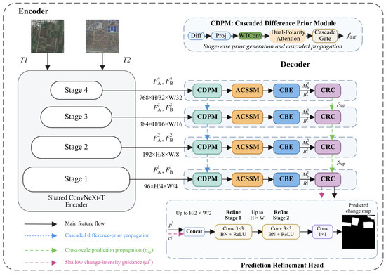
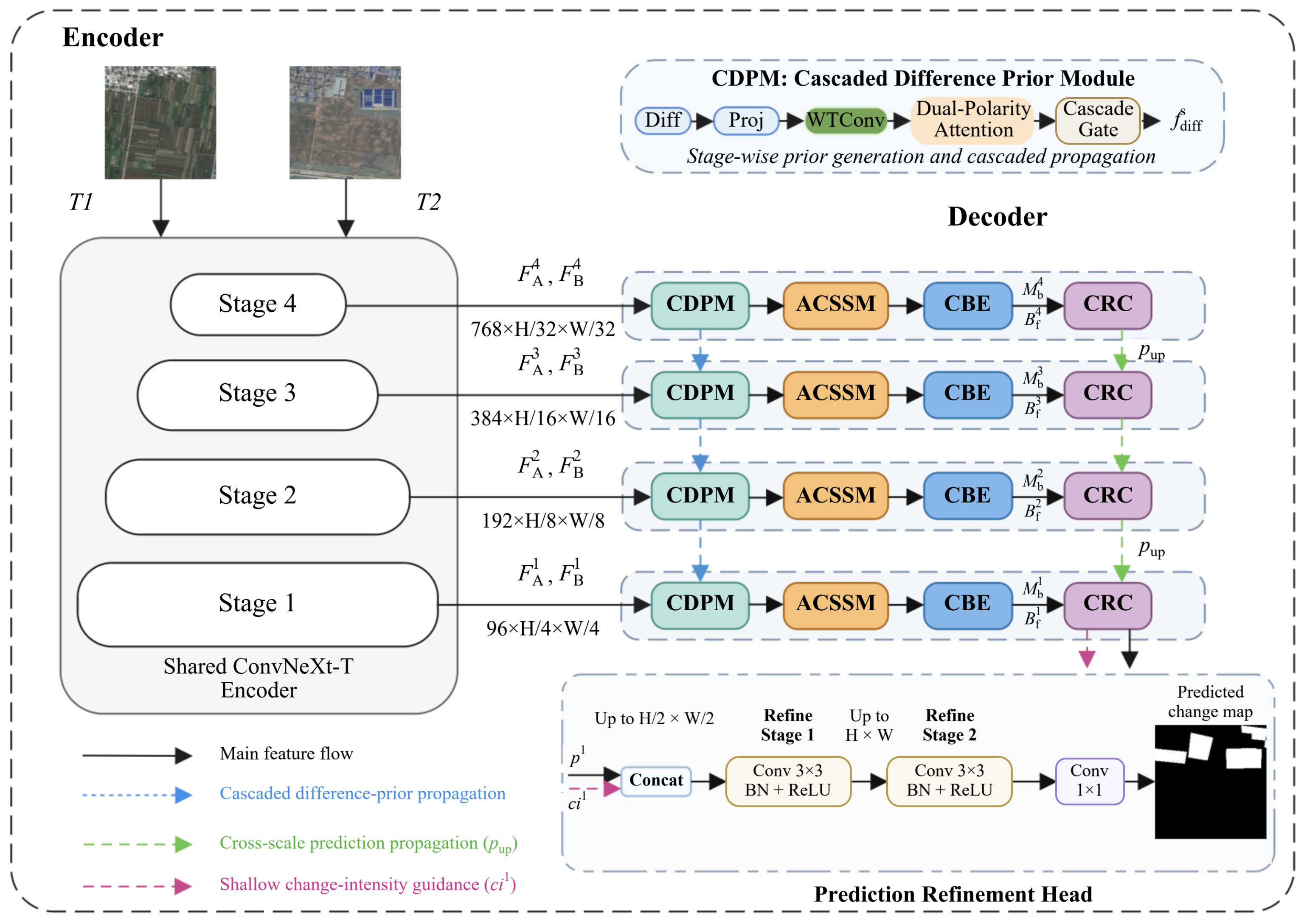
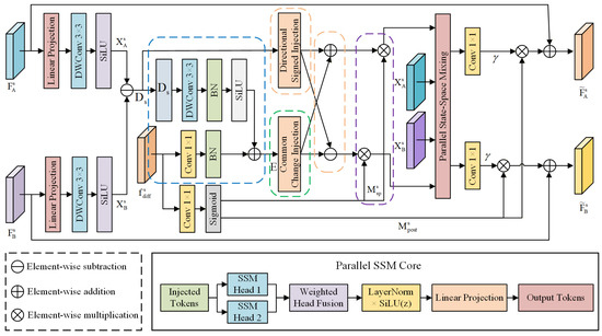
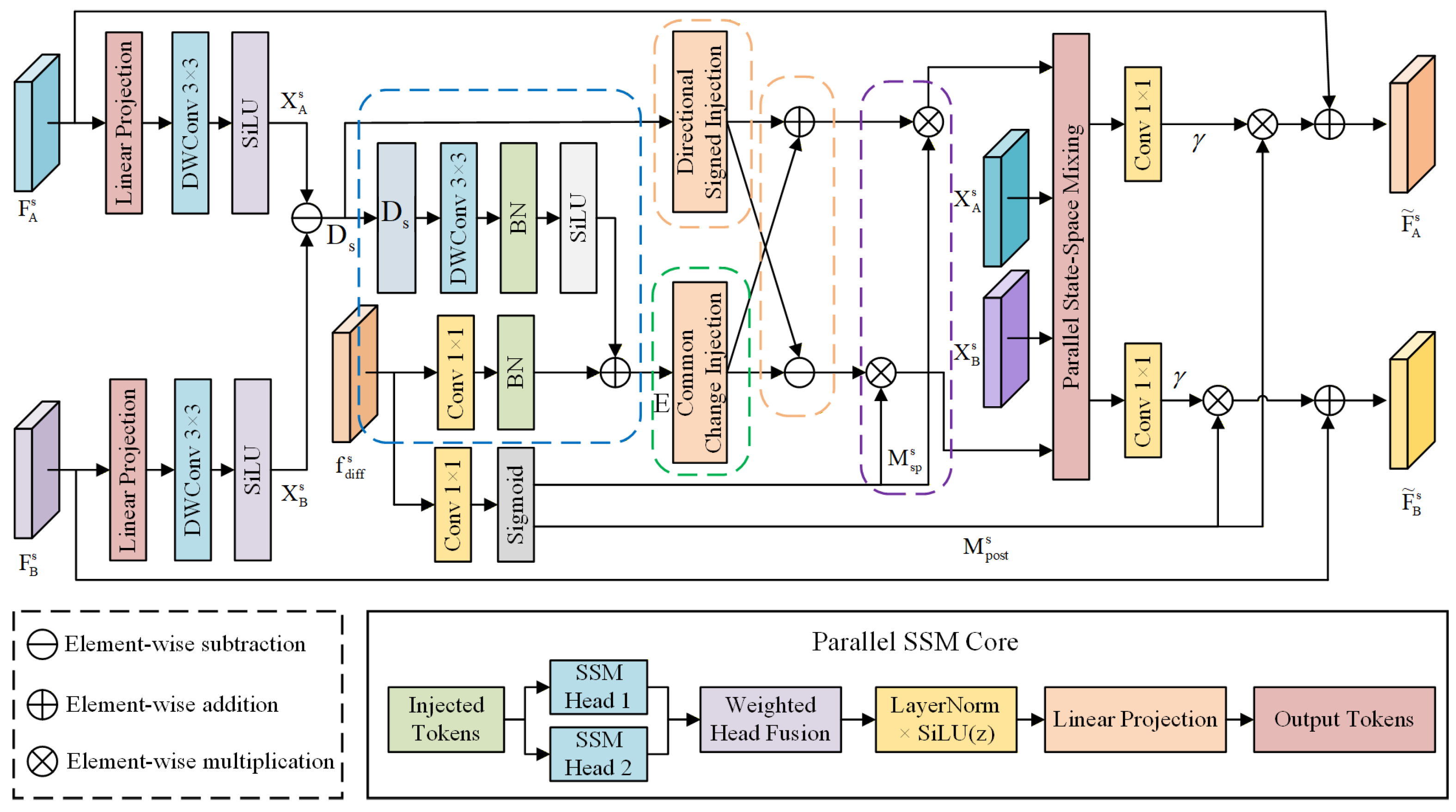
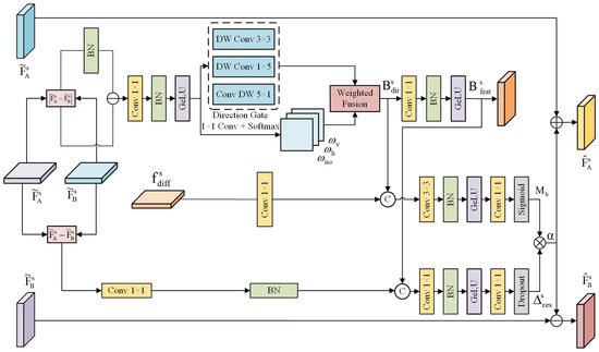
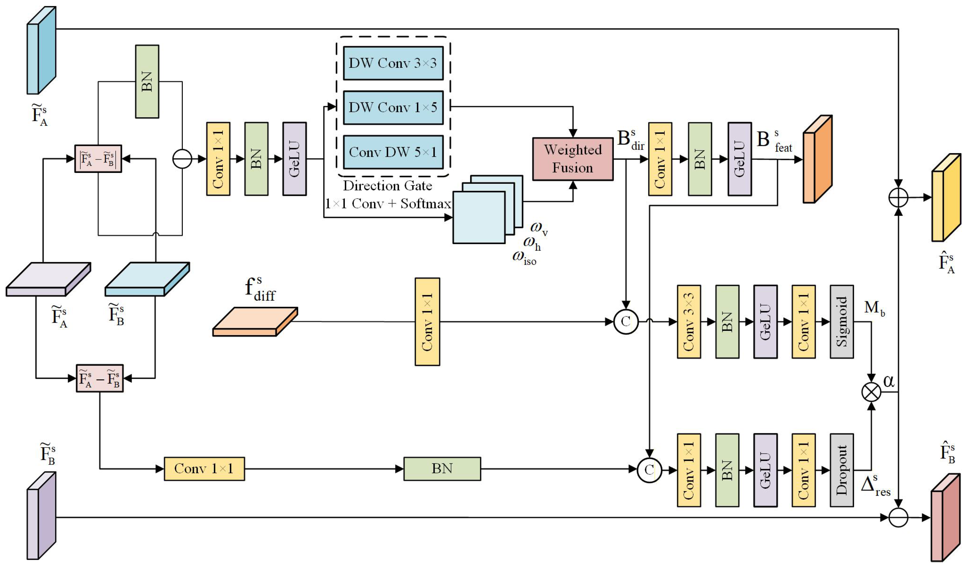
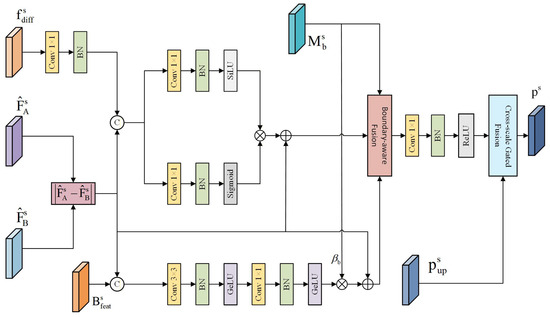
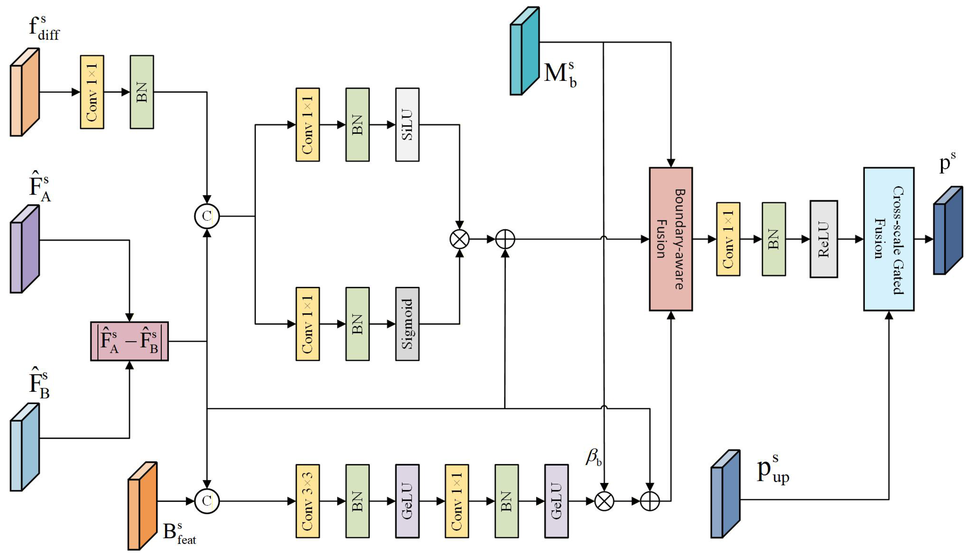
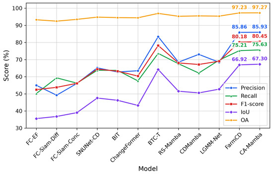
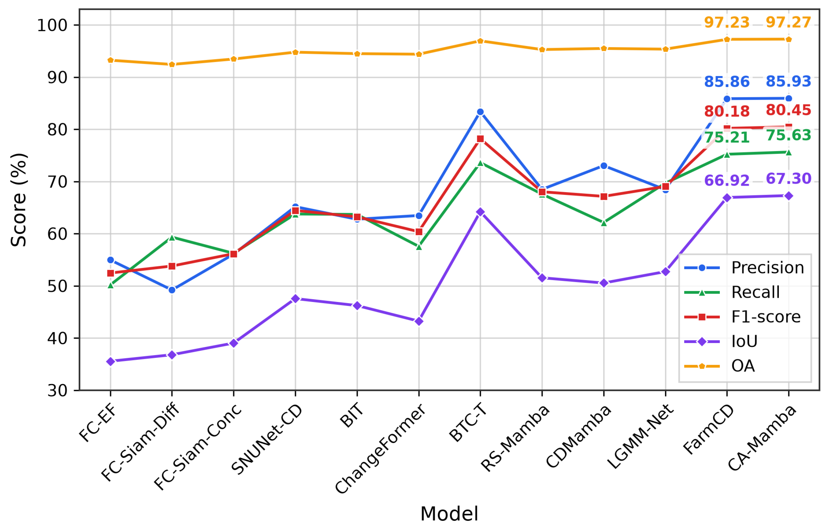
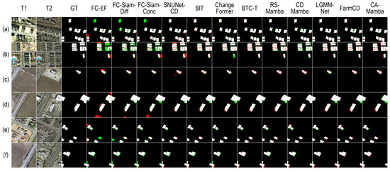
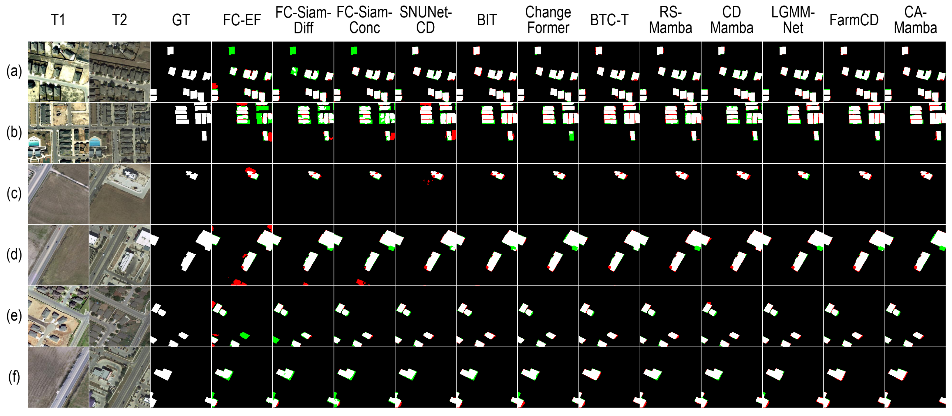
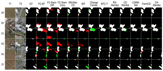
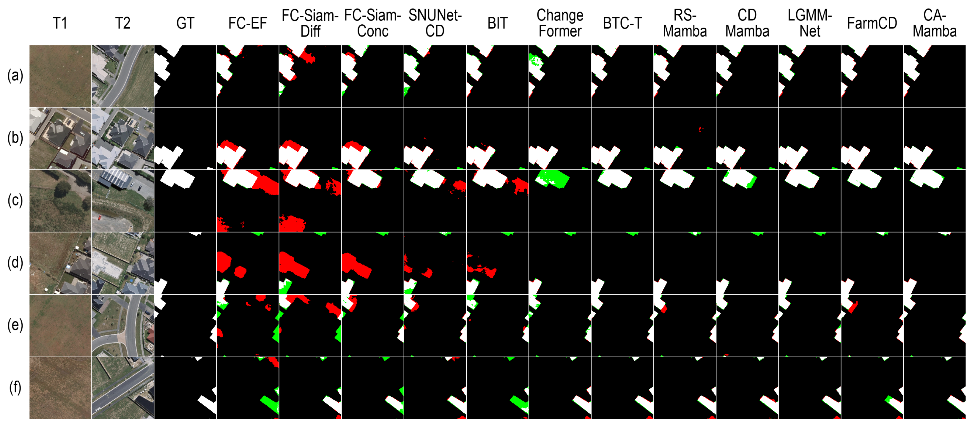
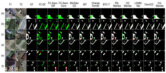
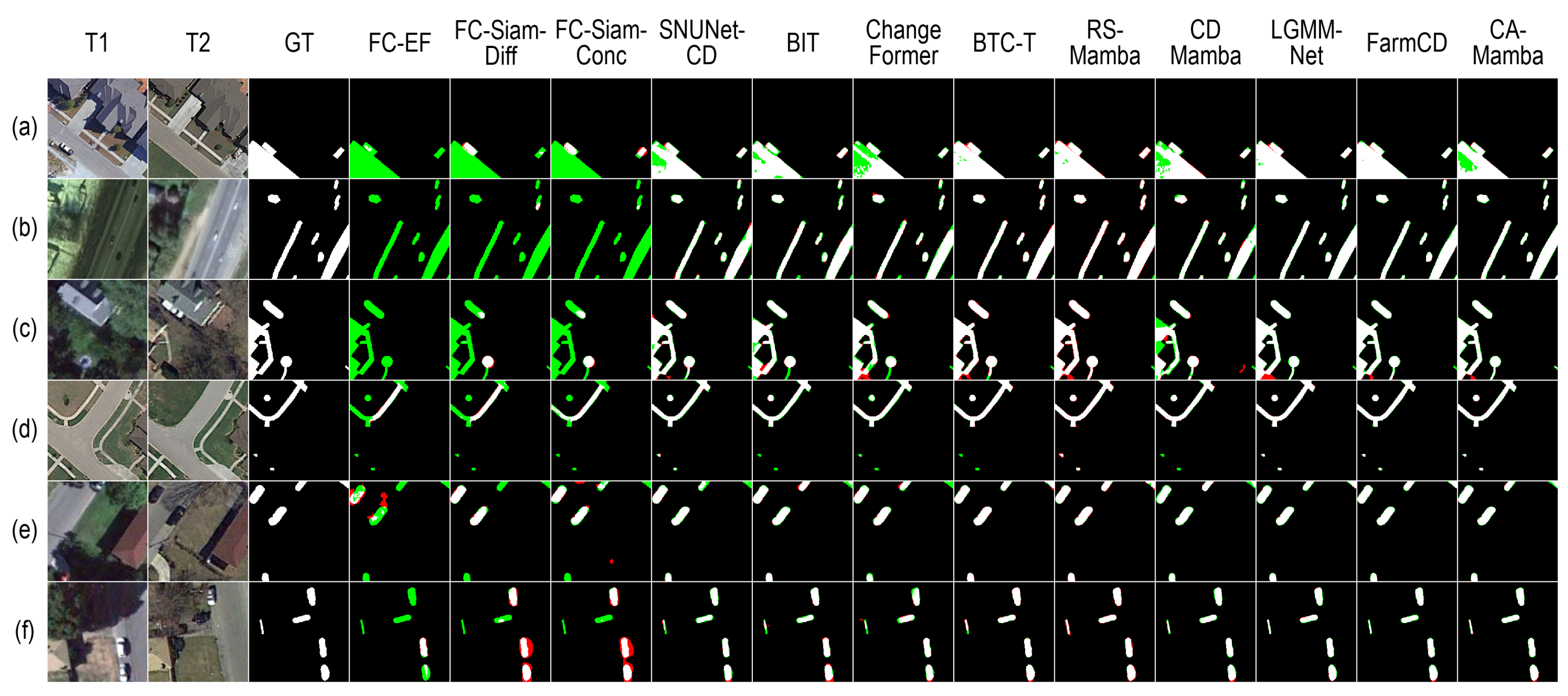
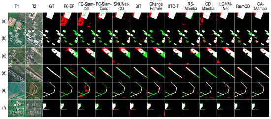
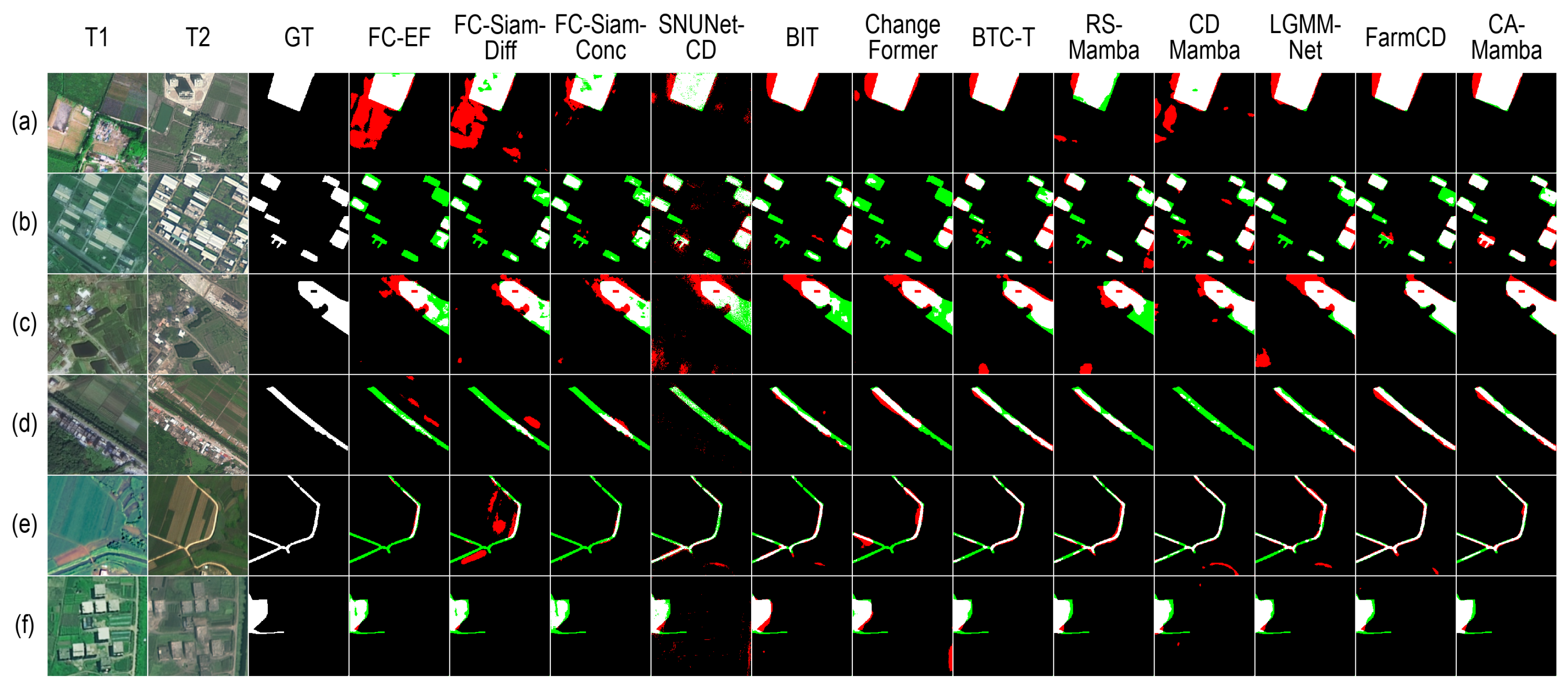
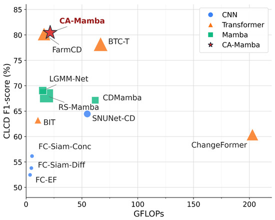
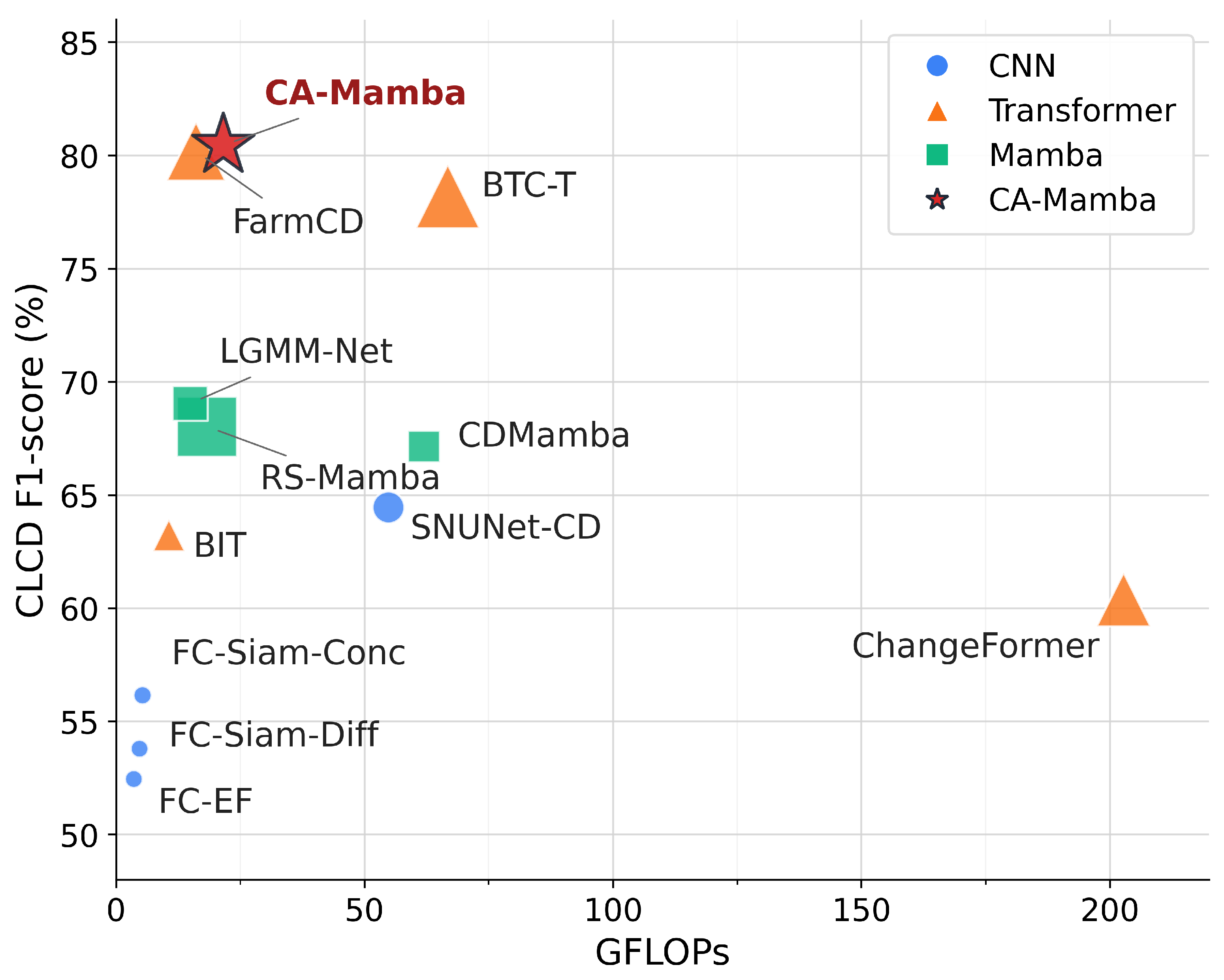
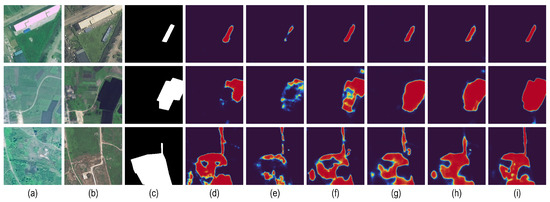
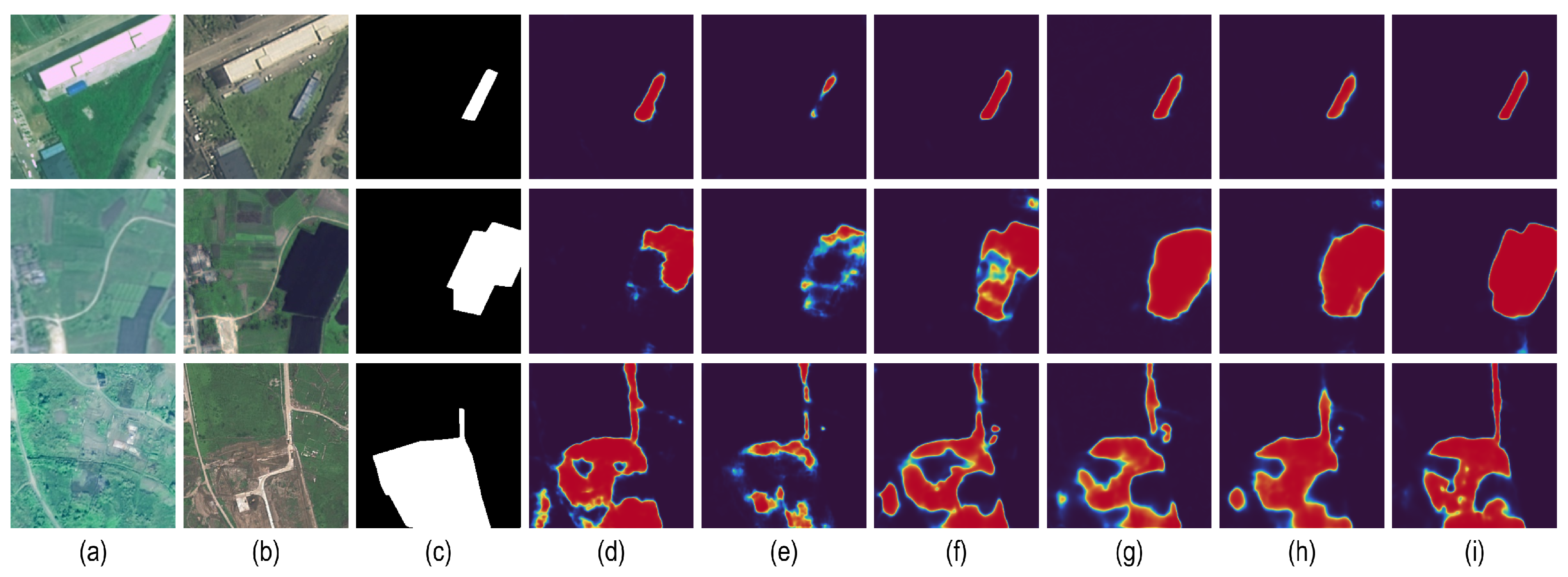

Disclaimer/Publisher’s Note: The statements, opinions and data contained in all publications are solely those of the individual author(s) and contributor(s) and not of MDPI and/or the editor(s). MDPI and/or the editor(s) disclaim responsibility for any injury to people or property resulting from any ideas, methods, instructions or products referred to in the content. |
© 2026 by the authors. Licensee MDPI, Basel, Switzerland. This article is an open access article distributed under the terms and conditions of the Creative Commons Attribution (CC BY) license.