


Highlights
What are the main findings?
- The First long-term (1990–2020) Landsat-based inventory of small and micro wetlands (SMWs) in Anhui Province was generated.
- SMWs expanded markedly after 2010, with increased patch-shape complexity but broadly stable connectivity and aggregation.
What are the implications of the main findings?
- Geodetector reveals temporally varying explanatory patterns and potential joint spatial associations among natural and anthropogenic factors.
- ESV increased markedly, with hydrological regulation among the dominant services.
Abstract
Comprehending the spatiotemporal dynamics, spatial heterogeneity, and pattern-process relationships of small and micro wetlands (SMWs) holds paramount significance for their conservation, restoration, and sustainable management. We integrated Landsat imagery, land-use, topographic, climatic, socioeconomic, and statistical data for 1990–2020 in Anhui Province. Random forest classification, kernel density estimation, standard deviation ellipses, centroid migration, landscape metrics, land-use transition analysis, ecosystem service value (ESV) assessment, and Geodetector were used to characterize SMW change. Total SMW area increased from 53,843.67 ha in 1990 to 71,637.39 ha in 2020, while patch number increased from 104,011 to 125,971; patches smaller than 3 hm2 remained dominant. High-density areas were concentrated in the Jianghuai Plain, Yangtze River plain, Chaohu Lake region, and agricultural drainage networks, with a persistent northeast–southwest distribution orientation. Land-use transitions were dominated by exchanges among cropland, water bodies, and SMWs. At constant 2020 grain prices, total ESV increased from approximately CNY 3.668 billion in 1990 to CNY 6.840 billion in 2020, with hydrological regulation remaining among the largest service components. Geodetector results showed temporally varying single-factor spatial associations, while interaction patterns suggested potential joint spatial associations among natural and anthropogenic factors. These results support spatially targeted SMW conservation and management in Anhui Province.
1. Introduction
Small and micro wetlands (SMWs) are generally characterized by small patch size, scattered distribution, and close associations with surrounding water systems and land-use backgrounds. Recent studies have emphasized that small wetlands can provide multiple ecosystem services and enhance the connectivity and stability of wetland ecological networks in highly urbanized landscapes [1]. In the study of Wuxi, Zhang et al. [2] identified SMWs as small-scale wetland units embedded within urban areas, agricultural landscapes, and lake-margin environments. Zhai et al. [3] further indicated that SMWs in the Yellow River Basin are commonly associated with agricultural drainage networks, riparian zones, ponds, ditches, and seasonal inundation areas. Y. Wang et al. [4] also demonstrated that SMWs in high-latitude regions are characterized by small patch size, spatial dispersion, and high sensitivity to environmental changes.
Although individual patches are usually limited in area, SMWs have considerable ecological significance. Atkinson et al. [5] found that small isolated wetlands are closely related to amphibian diversity, abundance, and nutrient export based on long-term monitoring. Biggs et al. [6] emphasized that small water bodies make important contributions to biodiversity conservation and ecosystem services. Cheng et al. [7] further demonstrated that small ephemeral wetlands can play a disproportionately large role in landscape-scale nutrient retention, while Kim et al. [8] revealed the importance of small wetlands in shaping ecological network transitions within wetland landscapes. Meanwhile, Mao et al. [9] showed that conversions between natural wetlands and cropland are closely associated with agricultural land use and wetland loss in China. Fluet-Chouinard et al. [10] further indicated that global wetlands have experienced extensive losses over the past three centuries. Therefore, understanding the long-term dynamics of SMWs is essential for assessing regional wetland-resource changes, ecological-function responses, and conservation-management needs.
SMWs data acquisition has progressed from field surveys and manual interpretation to remote sensing monitoring and spatial modelling. Zhang et al. [2] extracted SMWs in Wuxi using Landsat imagery, MNDWI, NDVI, and support vector machine classification, demonstrating the applicability of medium-resolution remote sensing for monitoring SMW dynamics in urban agglomerations. Gxokwe et al. [11] mapped small seasonal wetlands in semi-arid South Africa using the Google Earth Engine platform, highlighting the advantages of cloud-computing platforms for large-scale wetland identification. Peña-Regueiro et al. [12] used Sentinel-2 imagery to characterize the surface-water features of small wetlands, indicating that higher-spatial-resolution imagery can improve the delineation of recent small water body boundaries. Recent wetland studies have also shown that remote sensing-derived ecological indicators can effectively support wetland mapping and assessment, including indicators related to water bodies, vegetation, impervious surfaces, and landscape conditions [13]. In addition, water-related indices have been widely used to characterize hydrological conditions and surface-water dynamics in floodplain wetlands [14]. Random forest-based models have also been applied in wetland change simulation and have shown good capability in handling multi-source spatial variables [15]. Therefore, constructing long-term water body datasets from Landsat imagery and integrating water indices, vegetation indices, topographic variables, and machine-learning methods provides a feasible approach for identifying SMW patches at the provincial scale.
After obtaining spatial data on SMWs, changes in area, patch structure, land-use transition, ecosystem service value, and driving mechanisms are important for interpreting their ecological processes. Landscape metrics have been widely used to characterize wetland landscape pattern changes, including changes in patch structure, spatial configuration, and landscape heterogeneity [16,17]. In the field of SMWs research, Zhai et al. [3] explained the spatial dynamics and land-use context of SMWs in the Yellow River Basin through size-class structure, buffer analysis, and overlay analysis, while Y. Wang et al. [4] analyzed their spatiotemporal variation and multiple responses to driving factors in a high-latitude region. Land-use transition analysis provides an important basis for identifying the sources and destinations of wetland change, and ESV assessment can further reveal the ecological value response associated with land-use/cover change in wetland regions [18,19]. In terms of driving mechanisms, Li et al. [20] indicated that long-term wetland changes on the Tibetan Plateau showed clear responses to climate change. Johnston and McIntyre [21] found that cropland encroachment can alter the number, density, size, shape, and structural connectivity of prairie pothole wetlands. Jouma and Dadaser-Celik [22] also showed that irrigation development can reshape semi-arid wetlands and their surrounding landscape patterns. The Geodetector model has been used to distinguish the relative contributions and interactions of natural and anthropogenic factors in explaining spatial ecological heterogeneity [23]. Recent wetland ESV studies have also shown that ESV changes are closely related to wetland type evolution, service composition, land-use change, and driving factors [24]. These studies provide methodological support for linking land-use transition, landscape pattern evolution, ecosystem service value response, and associated factors in SMWs research.
Anhui Province is located in the eastern monsoon region of China and spans several major river systems, including the Huaihe River, the Yangtze River, and the Xin’an River. Plains, hills, and mountains coexist within the province, and lakes, rivers, and agricultural drainage networks are well developed, providing diverse geomorphological and hydrological conditions for the formation and evolution of SMWs. Since 1990, Anhui Province has experienced urban expansion, adjustments in agricultural land-use practices, water-conservancy construction, and changes in ecological protection policies. As a result, SMWs may exhibit regionally differentiated changes in area, patch reorganization, and land-use conversion. However, existing studies on SMWs have mainly focused on urban agglomerations, river basins, or specific natural geographical regions. Comprehensive studies at the provincial scale that simultaneously integrate area and quantity changes, size-class structure, landscape patterns, land-use transitions, ecosystem service value, and driving factors remain relatively limited. Therefore, it is necessary to integrate long-term remote sensing identification with multi-dimensional spatial analysis and ecological evaluation to better understand the evolution of SMWs in terms of spatiotemporal changes, landscape reorganization, land-use transition, ecosystem service responses, and driving mechanisms.
Based on this background, this study selected 1990, 1995, 2000, 2005, 2010, 2015, and 2020 as the study years. Annual water body information was extracted from Landsat imagery using the random forest classification method, and SMWs patches were identified by integrating area thresholds, morphological characteristics, and auxiliary hydrographic constraints. The study aimed to: (1) characterize changes in the area, number, size-class structure, and spatial aggregation of SMWs; (2) analyze landscape pattern evolution, centroid migration, and directional distribution; (3) identify land-use conversion relationships and evaluate ecosystem service value responses; and (4) quantify the explanatory power and interactions of natural and anthropogenic factors using the Geodetector model. The results can provide scientific support for SMWs conservation and restoration, agricultural drainage-network management, and territorial ecological regulation in Anhui Province.
2. Materials and Methods
2.1. Study Area
Anhui Province, situated in eastern China within the western Yangtze River Delta, spans approximately 114°54′–119°37′E and 29°41′–34°38′N, encompassing the North China Plain, Jianghuai hilly region, and southern Anhui mountains. Its terrain generally descends from higher elevations in the west and south to lower elevations in the north, with the south dominated by mountains and hills, the central region by the Jianghuai hills and Yangtze plains, and the north by the Huaibei Plain. The province has a dense hydrological network, including the Yangtze, Huaihe, and Xin’an rivers, as well as lakes such as Chaohu, Shengjin, and Wanfo, which provide a fundamental hydrological setting for SMWs. Climatically, it lies in a transitional zone between warm temperate and subtropical regimes, strongly influenced by the East Asian monsoon, with most precipitation concentrated in summer and showing marked interannual variability. SMWs are widely distributed across plains, river–lake margins, agricultural drainage networks, and hilly zones, but are relatively sparse in parts of the southern mountainous areas where steep topography and slope erosion limit their development. The combined effects of diverse terrain, well-developed water systems, and intensive cropland use make Anhui Province a typical region for investigating the spatiotemporal dynamics and associated factors of SMWs (Figure 1).
Figure 1.
Location and land-cover characteristics of the study area in Anhui Province.
2.2. Data Sources
The data used in this study include remote sensing imagery, land-use data, topographic data, climatic data, socioeconomic data, and ecosystem service value (ESV) accounting data (Table 1). Remote sensing imagery was used to delineate the spatial distribution of SMWs. Land-use data were used to analyze the conversion relationships between SMWs and other land-use types. DEM and climatic data were employed to characterize the natural background conditions associated with the formation and maintenance of SMWs, while socioeconomic data were used to represent human activities and their spatial differences. The ESV accounting data included grain yield per unit area in Anhui Province, prices of major grain crops, and the equivalent coefficients of wetland ecosystem services, which were used to convert changes in small and micro wetland area into comparable monetary values.
Table 1.
Description of datasets used in this study.
To ensure spatial consistency among multi-source datasets, all raster and vector data were unified in terms of coordinate system, spatial resolution, and study-area boundary before analysis. Data preprocessing included clipping, resampling, raster alignment, and missing-value processing. These procedures were not treated as isolated technical steps; rather, they were conducted to ensure that subsequent SMWs identification, land-use overlay analysis, landscape metric calculation, and Geodetector analysis were all performed under the same spatial reference framework.
2.3. Research Workflow
This study was conducted by integrating SMWs identification, spatial pattern analysis, land-use transition analysis, ecosystem service value assessment, and driving-factor detection (Figure 2). The overall framework consisted of seven main steps: data preparation, SMWs identification, spatiotemporal change analysis, landscape pattern analysis, land-use transition analysis, ecosystem service value assessment, and Geodetector-based driving factor analysis.
Figure 2.
Technical framework of the study.
First, annual waterbody information was extracted from multi-temporal Landsat imagery using the random forest classification method. SMW patches were then identified by combining area thresholds, morphological characteristics, existing hydrographic datasets, and visual verification based on high-resolution imagery. Subsequently, their spatial distribution and structural changes were characterized in terms of area, patch number, size-class structure, kernel density, centroid migration, standard deviation ellipse, and landscape pattern metrics.
On this basis, land-use transition matrices were used to identify the conversion relationships between SMWs and other land-use types, such as cropland, water bodies, and construction land. The equivalent-factor method was then applied to estimate changes in ecosystem service value. Finally, using the prefecture-level administrative units corresponding to each target year as the basic spatial units and SMWs area proportion as the dependent variable, the Geodetector model was applied to quantify the relative explanatory power and pairwise interactions of natural environmental and anthropogenic factors associated with the spatial differentiation of SMWs.
2.3.1. Image Preprocessing
To improve the comparability of annual water-body classification, Landsat Collection 2 Level-2 surface-reflectance data were used to construct annual image composites. For each target year, all valid Landsat observations acquired between 1 May and 31 October were selected to cover the main growing season and to reduce the influence of short-term hydrological variability associated with individual scenes. Dilated clouds, clouds, cloud shadows, and snow were masked using the QA_PIXEL band, and the surface-reflectance bands were converted using the Collection 2 scale factor and offset. For Landsat 5/7, SR_B1, SR_B2, SR_B3, SR_B4, SR_B5, and SR_B7 were mapped to Blue, Green, Red, NIR, SWIR1, and SWIR2, respectively; for Landsat 8, the corresponding bands were SR_B2, SR_B3, SR_B4, SR_B5, SR_B6, and SR_B7. All valid observations within the annual time window were then merged, and a pixel-wise median composite was generated to reduce the effects of residual cloud contamination, anomalous observations, and missing data from individual scenes.
Water-related and vegetation-related spectral indices were used to characterize surface-water conditions, wetland vegetation, and mixed pixels. Water-related indices have been widely used to characterize hydrological conditions and surface-water dynamics in floodplain wetlands [14], while Sentinel-2-based studies have also shown that spectral information can improve the delineation of small water bodies in wetland environments [12]. In this study, NDWI, MNDWI, and AWEI were used to enhance open-water information and suppress background interference under complex surface conditions, while NDVI and EVI were used to characterize vegetation-cover conditions and wetland vegetation responses. The main spectral indices used in this study were calculated as follows:
where , , , , , and represent the surface reflectance values of the blue, green, red, near-infrared, first shortwave-infrared, and second shortwave-infrared bands after radiometric and atmospheric correction, respectively. For different Landsat sensors, the corresponding bands were extracted according to their spectral definitions, and all index layers were resampled and aligned to the same spatial resolution and study-area boundary before participating in subsequent random forest classification.
For Landsat 7 ETM+ imagery acquired after the Scan Line Corrector failure (SLC-off), no additional spatial interpolation or artificial gap-filling procedure was applied. Instead, invalid observations were excluded, and multi-scene median compositing within the annual time window was used to reduce the influence of scan-line gaps; where observations from other Landsat sensors were available for the same period, these valid observations were also included in the annual composite. To reduce cross-sensor differences among Landsat 5, 7, and 8, all images were processed from Collection 2 Level-2 surface-reflectance products using a common band-naming scheme, spatial resolution, feature set, and classification workflow. No additional empirical cross-sensor spectral harmonization was applied; therefore, residual differences in sensor spectral response may still affect the long-term comparison and are considered in the Discussion.
2.3.2. Extraction of Small and Micro Wetlands
Following previous studies [2,3], SMWs in this study were defined as small wetland patches with an area of less than 8 hm2 and with permanent or seasonal water occurrence. Previous studies have similarly used an area threshold of 8 hm2 and included both permanent and seasonal water occurrence in the identification of SMWs. Considering the complex hydrographic conditions in Anhui Province, including rivers, lakes, reservoirs, ditches, ponds, and agricultural drainage networks, the annual water-classification results may include non-target water bodies such as main river channels, large lakes, reservoir margins, artificial canals, and other engineered water surfaces. To improve the specificity of SMWs identification, a workflow of “annual water-body mapping–candidate-patch screening” was adopted.
First, annual water body classification was performed using Landsat imagery. Cloud, cloud-shadow, and low-quality observations were removed during image preprocessing. Reference samples from the permanent-water and non-water classes of the JRC Global Surface Water Yearly History dataset were then used to evaluate the consistency of the classification results [25], while seasonal-water and no-data classes were excluded from this assessment. Because the JRC product itself is primarily derived from Landsat observations, this assessment was treated as an external consistency evaluation rather than as fully independent accuracy validation. A classification feature set was constructed by integrating original spectral bands, water indices, vegetation indices, and terrain variables. Water-related and vegetation-related indices were used to enhance surface-water information, characterize vegetation conditions, and reduce the interference of mixed pixels under complex land-cover backgrounds [13,14]. DEM-derived slope was introduced to reduce the influence of terrain shadows and steep-slope areas on water body classification. In addition, the China Land Cover Dataset was used as an auxiliary source for training-sample construction [26]. Water and non-water samples were extracted and further refined through visual interpretation and high-resolution imagery. Random forest classification was applied because of its robustness in remote sensing classification and its ability to handle multi-source feature variables [27]. Training labels were derived from the contemporaneous China Land Cover Dataset (CLCD), with water and non-water classes used to construct the binary training samples. A maximum of 2500 candidate samples were randomly selected for each class and divided into training and testing subsets at a ratio of 70:30 using a random seed of 2024. The predictor set consisted of 12 variables, including six spectral bands (Blue, Green, Red, NIR, SWIR1, and SWIR2), five spectral indices (NDVI, NDWI, MNDWI, AWEI, and EVI), and terrain slope. The random forest classifier contained 150 trees, with a bag fraction of 0.7 and a random seed of 2024. Random forest-based models have also been applied in wetland change simulation and have shown good capability in handling multi-source spatial variables [15]. After classification, the water-body results were further constrained using spectral and terrain thresholds (MNDWI > −0.10, NDVI < 0.40, EVI < 0.25, AWEI > −0.10, NDWI > −0.10, and slope < 15°). An eight-neighbor connectivity filter was then applied, and isolated single-pixel detections were removed. At least two connected 30 m pixels were required to retain a water patch, corresponding to an effective minimum mapping unit of 0.18 hm2. This relatively small threshold was retained because genuine SMWs in the 0–1 hm2 class were an important target of the study. Patch area and spatial morphology were then calculated from the annual water body maps to support the identification of candidate SMWs patches.
Second, auxiliary hydrographic datasets were used to further exclude non-target water bodies such as large lakes, reservoirs, main river channels, and artificial water-conservancy facilities. Specifically, the ReaLSAT reservoir and lake surface area dataset was used to identify lake and reservoir water surfaces, while the China River Extent Maps (CRED) were used as a recent auxiliary river mask to assist in excluding main river-channel-related patches. These datasets were not used to analyze the temporal evolution of lakes, reservoirs, or rivers directly; rather, they served as auxiliary masks for refining candidate SMWs patches. For candidate patches associated with main irrigation and drainage canals, large artificial water bodies, and engineered ponds, manual interpretation was conducted based on regional hydrological characteristics, land-use context, and image texture features. In contrast, small ponds, ditch nodes, and persistent open-water patches within agricultural drainage networks were retained when they met the area threshold and exhibited relatively independent patch morphology. Through this procedure, the final SMWs dataset was obtained for subsequent spatiotemporal analysis.
To further evaluate the reliability of the final SMWs dataset after hydrographic exclusion and manual screening, an object-level stratified validation was conducted using the final 2020 SMWs dataset. A total of 120 mapped patches were randomly sampled according to four SMWs patch-size classes, including 50 samples from 0–1 hm2, 30 from 1–3 hm2, 20 from 3–5 hm2, and 20 from 5–8 hm2. Sentinel-2 imagery at 10 m spatial resolution was used as the primary source for visual interpretation. Google Earth historical high-resolution imagery was additionally consulted for samples that remained difficult to interpret. Each sample was classified as either a target small and micro wetland or a non-target feature based on patch morphology, surrounding land-use context, and water/wetland characteristics. Because all validation samples were drawn from mapped positive patches in the SMWs dataset, this assessment was used primarily to estimate user’s accuracy and commission error of the final SMWs dataset; overall accuracy and producer’s accuracy could not be derived from this positive-only sampling design.
2.3.3. Analysis of Patch Number, Area, and Spatial Distribution of Small and Micro Wetlands
The extracted multi-temporal SMWs datasets provided the basis for quantifying changes in patch number, total area, and size-class structure. These indicators were calculated for each target year to characterize changes in SMWs quantity and patch composition. To further describe patch-size composition, SMWs patches were divided into four area classes following Zhai et al. [3]: 0–1 hm2, 1–3 hm2, 3–5 hm2, and 5–8 hm2.
In terms of spatial distribution, this study analyzed the spatial evolution of SMWs from three dimensions: spatial clustering, distribution direction, and centroid migration. For the kernel density analysis, each SMW patch was converted to an internal representative point, and all patches were assigned equal weight. Kernel density estimation was performed in the Asia North Albers Equal Area Conic projection (WKID 102025) using a 500 m output cell size, a 10 km search radius, and planar distance. Density values were expressed as the number of patches per square kilometer. To ensure temporal comparability, the positive kernel-density values from all seven target years were pooled and classified into five levels using a common Jenks natural-break scheme, and the same class thresholds were applied to all years.
The standard deviational ellipse and mean-center analyses were also performed in the same equal-area projection. The standard deviational ellipse method has been applied to characterize the directional distribution and spatial migration of wetland landscapes [28]. Patch area was used as the weight for both the mean center and the standard deviation ellipse, and a one-standard-deviation ellipse was used to characterize the dominant distribution direction and spatial dispersion of SMWs. Centroid migration was then calculated between consecutive target years to quantify the direction and distance of the area-weighted spatial center of SMWs.
Kernel density estimation, centroid calculation, and centroid migration distance were calculated using Equations (4) and (5):
where is the search bandwidth, is the distance between patch i and location , is the area of patch i, and is the kernel function. and represent the centroid coordinates of patch i in year t, while represents its patch area. and denote the area-weighted centroid coordinates of small and micro wetlands in year t. When projected coordinates were measured in meters, the centroid migration distance was divided by 1000 and converted into kilometers.
2.3.4. Quantification of Landscape Pattern of Small and Micro Wetlands
Landscape pattern metrics were calculated at both the class and landscape levels. At the class level, SMWs were treated as the target class to characterize the evolution of their own landscape pattern. Six metrics were selected: class area (CA), number of patches (NP), patch density (PD), landscape shape index (LSI), patch cohesion index (COHESION), and aggregation index (AI). These metrics were used to describe changes in SMWs area, patch number, patch density, shape complexity, structural connectivity, and spatial aggregation.
At the landscape level, the entire study area and all land-cover classes were treated as the analysis unit to characterize changes in the overall regional landscape pattern. Four metrics were selected: patch density (PD), edge density (ED), contagion index (CONTAG), and Shannon’s diversity index (SHDI). These metrics represented overall patch density, edge complexity, spatial aggregation, and landscape diversity, respectively. Landscape metrics have been widely used to quantify changes in patch structure, spatial configuration, aggregation, connectivity, and landscape heterogeneity [16,17].
CA and NP were obtained directly from the total area and patch number of SMWs, respectively. Class-level PD, LSI, and AI were calculated using Equation (6), whereas landscape-level PD, ED, and SHDI were calculated using Equation (7). COHESION and CONTAG were calculated according to their standard landscape-metric definitions. For the class-level analysis, patch density was defined as the number of SMWs patches per 100 ha of SMWs area, whereas landscape-level PD represented the total number of patches per 100 ha of the entire landscape.
where is the number of patches of class i, is the total area of class i (m2), and is the total edge length of class i (m). is the number of like adjacencies between pixels of class i, and is the maximum possible number of like adjacencies for class i. N is the total number of patches across all land-cover classes, is the total landscape area (m2), and E is the total edge length of the landscape (m). is the proportional abundance of class i in the landscape, and m is the total number of land-cover classes. PD is expressed as the number of patches per 100 ha, whereas ED is expressed as m/ha.
2.3.5. Land-Use Transition Analysis
While the previous analyses described changes in SMWs area, spatial distribution, and landscape structure, land-use transition matrices were used to identify the sources and destinations of SMWs change. The matrices were constructed using the SMWs datasets and land-use data. They were used to analyze the conversion relationships between SMWs and other land-use types during adjacent periods. The transition matrix can quantify the area transferred into and out of different land-use categories between adjacent periods and has been widely used to analyze wetland change and its associated land-use background [9,29]. Compared with simple area-change statistics, the transition matrix can further identify the main source and destination land-use types of SMWs expansion, loss, and transformation.
In this study, land-use transition matrices were constructed for six periods: 1990–1995, 1995–2000, 2000–2005, 2005–2010, 2010–2015, and 2015–2020. The analysis focused on three aspects: (1) conversions from other land-use types to SMWs, which were used to identify the sources of SMWs expansion; (2) conversions from SMWs to other land-use types, which were used to identify the main directions of SMWs loss or transformation; and (3) mutual conversions between SMWs and major land-use types, such as cropland, construction land, and water bodies. To ensure consistency between the mapped SMW datasets and the land-use transition analysis, the final SMWs raster for each target year was aligned with the corresponding land-use raster at a 30 m resolution. Pixels identified as SMWs were recoded as an independent class (class 10), replacing the original land-use category at the same locations, while all remaining pixels retained their original land-use classes. This procedure allowed SMWs to be treated as an independent category in the spatial transition analysis. All annual rasters were standardized to the same spatial extent and grid alignment before the transition analysis.
The land-use transition matrix was used to quantify the area conversion relationships among different land-use types between adjacent periods. Its basic form is expressed as follows:
where represents the area converted from land-use type i in period t to land-use type j in period t + 1, and denotes the corresponding transition proportion.
2.3.6. Ecosystem Service Value Assessment of Small and Micro Wetlands
Changes in SMWs area and land-use transitions may further affect wetland ecosystem services. Therefore, the ecosystem service value (ESV) equivalent-factor method was applied to evaluate the ecological value response of SMWs. The calculation integrated SMWs area, grain yield, grain price, and wetland value-equivalent coefficients. Following the equivalent-factor method developed for ecosystem service valuation in China [30], this study calculated the ESV of SMWs by integrating SMWs area, grain yield, grain price, and wetland value-equivalent coefficients. Recent studies have also applied this method to assess ESV changes in lake-wetland and urban wetland regions based on land-use change and wetland type evolution [18,24].
To reduce the influence of interannual price fluctuations and improve temporal comparability, the value of one standard equivalent factor was calculated using grain yield per unit area and the average grain price in Anhui Province. Following Xie et al. [30], one standard equivalent factor was defined as one-seventh of the annual economic value of grain production per unit area:
is the value of one standard equivalent factor in year t (CNY/hm2), is the grain yield per unit area in year t (kg/hm2), and is the average grain price in year t (CNY/kg). Rice, wheat, and maize were selected as the main grain crops, and the weighted average grain price was calculated as follows:
, , and represent the prices of rice, wheat, and maize in year t, respectively, and , , and denote their corresponding yields. When the prices of early-season, middle-season, and late-season rice were available, the rice price was calculated as their arithmetic mean:
After obtaining the value of one standard equivalent factor, the ESV of SMWs was calculated using wetland ecosystem service equivalent coefficients. According to the ecosystem service classification framework of Xie et al. [30], wetland ecosystem services were divided into 11 categories: food production, raw material production, water supply, gas regulation, climate regulation, environmental purification, hydrological regulation, soil conservation, nutrient cycling maintenance, biodiversity maintenance, and aesthetic landscape. The ESV of service type i in year t was calculated as follows:
represents the value of ecosystem service type i in year t, with the unit of 108 CNY; represents the total ESV of small and micro wetlands in year t, also with the unit of 108 CNY; is the total area of small and micro wetlands in year t, with the unit of hm2; and is the equivalent coefficient of ecosystem service type i.
To further analyze city-scale differences in the ESV of SMWs, this study calculated the ESV for each prefecture-level city. City-scale ESV statistics followed the prefecture-level administrative configuration corresponding to each target year. Chaohu was treated as an independent prefecture-level city through 2010 but was not reported separately in 2015 or 2020 following the 2011 administrative reorganization. The same provincial-level value coefficient was used for all cities in the same year to ensure comparability among regions. Therefore, spatial differences in city-scale ESV mainly reflected differences in the area and distribution of SMWs. Considering that raster clipping, administrative boundaries, and patch attribution may lead to slight inconsistencies between the summed city-level area and the provincial total area, city-scale SMWs area was proportionally normalized to ensure that the sum of city-level ESV was consistent with the provincial total ESV:
is the normalized area of small and micro wetlands in city c in year t, with the unit of hm2; is the original statistical area of small and micro wetlands in city c in year t, with the unit of hm2; is the total area of small and micro wetlands in Anhui Province in year t, with the unit of hm2; and m is the number of prefecture-level cities.
The total ESV and service-specific ESV of small and micro wetlands in city c in year t were calculated as follows:
represents the total ESV of small and micro wetlands in city c in year t, with the unit of 108 CNY; represents the value of ecosystem service type i in city c in year t, with the unit of 108 CNY; is the sum of the equivalent coefficients of the 11 ecosystem service types; and is the equivalent coefficient of ecosystem service type i. The city-scale ESV results were used to compare spatial differences and temporal changes in the ecosystem service value of small and micro wetlands among prefecture-level cities in Anhui Province.
2.3.7. Geodetector-Based Driving Factor Analysis
The preceding analyses revealed the spatiotemporal changes, landscape structure, land-use transitions, and ESV responses of SMWs. The Geodetector model was further used to identify the factors influencing the spatial differentiation of SMWs. It was also used to quantify interactions between natural and anthropogenic factors. The Geodetector model can quantify the explanatory power of independent variables for the spatial heterogeneity of a dependent variable without requiring a linear assumption, and can further detect interactions among different factors [31,32].
In this study, the prefecture-level administrative units corresponding to each target year in Anhui Province were used as the basic spatial units, and the proportion of SMW area relative to the total area of each administrative unit was used as the dependent variable to reduce the influence of differences in administrative-unit size. Nine explanatory variables were considered, including DEM, annual mean NDVI, annual precipitation, annual mean temperature, population density, GDP per capita, annual mean nighttime light, cropland area, and built-up area. DEM, NDVI, annual precipitation, and annual mean temperature represented natural and ecological environmental conditions, whereas population density, GDP per capita, annual mean nighttime light, cropland area, and built-up area characterized human activity intensity and land-use background.
To meet the requirement of categorical variables in the Geodetector model, continuous explanatory variables were discretized into four classes using the natural breaks method, namely high, medium-high, medium-low, and low classes. The discretized factors were then matched with SMWs area at the prefecture-level city scale. Since the discretization of continuous variables may influence q-value estimation, the subsequent interpretation mainly focused on relative explanatory power and interaction relationships [32,33].
The factor detector was used to measure the explanatory power of each factor for the spatial differentiation of SMWs. The q statistic was calculated as follows:
H represents the stratum of the dependent or explanatory variable, L is the number of strata, and N are the numbers of samples in stratum h and the entire study area, respectively, and and are the variances within stratum h and the entire study area, respectively. The q-value ranges from 0 to 1. A larger q-value indicates stronger explanatory power of the factor for the spatial differentiation of small and micro wetlands. The interaction detector was used to determine whether two factors jointly enhanced or weakened their explanatory power by comparing q(), q(), and q( ∩ ). If q( ∩ ) is greater than the q-values of the two individual factors, the interaction is considered to have an enhancement effect.
Statistical support for the factor- and interaction-detector results was assessed separately for each target year using permutation tests. During each test, SMWs area-proportion values were randomly reassigned among prefecture-level spatial units while the stratification of the explanatory variables remained unchanged, and the corresponding q statistic was recalculated. Each test was repeated 9999 times. The permutation p-value was estimated as the proportion of randomized q-values equal to or greater than the observed q-value. Because multiple factors and factor combinations were examined within the same year, the resulting p-values were further adjusted using the Benjamini–Hochberg false discovery rate (FDR) procedure. An adjusted p-value < 0.05 was considered statistically significant. The robustness of q-values to the discretization scheme was further examined using three-, four-, and five-class Jenks natural-break classifications. The four-class scheme was retained for the main analysis, whereas the three- and five-class schemes served as sensitivity checks. In addition, the number of spatial units within each single-factor and interaction stratum was recorded to identify sparse stratification. Because some interaction strata contained only one spatial unit, interaction q-values were interpreted cautiously as exploratory indicators of joint spatial association rather than as direct evidence of causal synergy.
3. Results
3.1. Extraction and Spatial Analysis of Small and Micro Wetlands
The JRC-based consistency assessment showed that the overall accuracy (OA) of the candidate water-body classification ranged from 0.89 to 0.98 across the seven target years, while the Kappa coefficient ranged from 0.78 to 0.95 and water-class precision ranged from 0.90 to 0.98. The corresponding multi-year mean values were 0.95, 0.89, and 0.95, respectively (Table 2). Because the JRC Global Surface Water product is itself primarily derived from Landsat observations, these results mainly represent consistency between the annual water-body maps produced in this study and an existing long-term surface-water product.
Table 2.
Accuracy assessment of candidate water bodies smaller than 8 hm2 in the target years.
To further assess the reliability of the final SMWs dataset, an object-level stratified validation was conducted using the final 2020 SMWs data. Among the 120 randomly selected mapped-positive samples, 105 were confirmed as target small and micro wetlands using high-resolution remote-sensing imagery, corresponding to an overall positive-class user’s accuracy of 87.5%, with a Wilson 95% confidence interval of 80.4–92.3%. The class-specific user’s accuracies were 86.0%, 96.7%, 75.0%, and 90.0% for the 0–1, 1–3, 3–5, and 5–8 hm2 classes, respectively (Table 3). Overall, the final SMWs dataset showed satisfactory object-level identification consistency, although some uncertainty remained for small or morphologically complex patches.
Table 3.
A Size-class-specific accuracy assessment of the final 2020 small and micro wetlands dataset.
The size-class structure of SMWs reflects their patch-size composition and regional differences. Based on the extracted wetland patches in 1990, 1995, 2000, 2005, 2010, 2015, and 2020, this study divided SMWs into four size classes: 0–1 hm2, 1–3 hm2, 3–5 hm2, and 5–8 hm2. The size-class composition of each prefecture-level city was represented by pie charts and overlaid on the administrative map to visualize the spatial differences in wetland patch-size structure from 1990 to 2020 (Figure 3). As shown in Figure 3, the size-class composition of SMWs in Anhui Province remained generally consistent from 1990 to 2020. Patches of 0–1 hm2 dominated in all years, followed by those of 1–3 hm2, whereas the proportions of 3–5 hm2 and 5–8 hm2 patches were relatively low. This indicates that SMWs in Anhui Province were mainly composed of small-area patches, whereas patches in the 3–5 hm2 and 5–8 hm2 classes accounted for only a limited proportion. At the regional scale, the size-class composition varied among cities. In areas with relatively dense river networks and agricultural drainage systems, SMWs were more concentrated, and the patch composition was relatively diverse. By contrast, in mountainous and hilly areas or regions with sparse water systems, SMW patches were fewer and more scattered. In general, the size-class composition of SMWs in Anhui Province was dominated by the 0–1 hm2 and 1–3 hm2 classes during 1990–2020. Although the proportions of different size classes fluctuated slightly among cities and years, no fundamental shift in the overall size-class structure was observed. This suggests that the long-term changes in SMWs were reflected not only in area increase or decrease, but also in the spatial reorganization and local adjustment of existing small patches. In general, SMWs in Anhui Province were characterized by small patch size and a stable dominant size-class structure, while certain regional differences remained in their spatial composition.
Figure 3.
Changes in the spatial distribution and size-class composition of small and micro wetlands in Anhui Province from 1990 to 2020: (a) 1990; (b) 1995; (c) 2000; (d) 2005; (e) 2010; (f) 2015; and (g) 2020. The pie charts represent the area proportions of four size classes of small and micro wetlands in each prefecture-level city.
To gain a more comprehensive understanding of the spatiotemporal changes in SMWs in Anhui Province, this study examined the interannual variations in total area, patch number, regional area composition, and size-class structure from 1990 to 2020. The seven target years, namely 1990, 1995, 2000, 2005, 2010, 2015, and 2020, were used to characterize the temporal trajectory of SMWs over the past three decades.
The examination of changes in total area showed a fluctuating but overall increasing trend (Figure 4a). The total area decreased from 53,843.67 ha in 1990 to 43,941.33 ha in 1995, and remained at a relatively low level in 2000. A short-term increase was observed in 2005, when the area reached 50,167.08 ha, followed by another decline to 44,131.32 ha in 2010. After 2010, the area increased continuously, reaching 62,417.25 ha in 2015 and 71,637.39 ha in 2020. Compared with 1990, the total area of SMWs increased by 17,793.72 ha in 2020, representing an increase of approximately 33.0%. These results indicate that the area change of SMWs in Anhui Province did not follow a simple linear trend, but was characterized by an early decline, mid-period fluctuation, and later expansion.
Figure 4.
Changes in the area and patch number of small and micro wetlands in Anhui Province from 1990 to 2020: (a) total area; (b) patch number.
The change in patch number showed a similar but not identical temporal pattern (Figure 4b). The number of SMW patches decreased from 104,011 in 1990 to 88,046 in 1995, and further declined to 81,437 and 81,153 in 2000 and 2005, respectively. In 2010, the patch number reached its minimum value of 74,752, indicating that both wetland area and patch number were at relatively low levels during this period. After 2010, the number of patches increased markedly, reaching approximately 9.4 × 10⁴ in 2015 and 1.26 × 10⁵ in 2020. Compared with 2010, the patch number increased by about 5.1 × 10⁴ in 2020, with an increase of approximately 68%. This suggests that the post-2010 expansion was not only reflected in total area recovery, but also in the reappearance or formation of numerous small patches.
Notably, both total area and patch number reached relatively low values in 2010, indicating a period of substantial contraction and patch loss. The land-use transition results further showed that SMWs experienced a net decrease of 99.20 km2 during 2005–2010, suggesting that outward conversion exceeded inward conversion during this period. In addition, the Geodetector results indicated that the explanatory power of annual precipitation reached 0.5380 in 2010, implying a close relationship between SMWs distribution and climatic–hydrological conditions in that year. Therefore, the low values observed in 2010 may be associated with seasonal waterbody shrinkage, low-water conditions, and the conversion of some small wetland patches into dryland or general waterbody categories.
After regional stratification, the area changes in northern, central, and southern Anhui all showed phased fluctuations from 1990 to 2020 (Figure 5a–c). In northern Anhui, the area of SMWs decreased from 1990 to 2000, remained relatively low around 2000–2010, and then increased significantly after 2015, reaching a high level in 2020. Central Anhui showed a similar trend of early decline and later increase, with relatively low values in 2000 and 2010 and a clear increase after 2015. In southern Anhui, the changes were more fluctuating, with relatively high values in 1995 and 2015 and lower values in 2000 and 2010. These regional changes were generally consistent with the provincial-scale trend shown in Figure 4, indicating that the decline around 2000 and 2010 and the subsequent increase after 2015 were not confined to a single region, but occurred across northern, central, and southern Anhui.
Figure 5.
Regional area structure and size-class composition of small and micro wetlands in Anhui Province from 1990 to 2020: (a) area composition of small and micro wetlands in northern Anhui; (b) area composition in central Anhui; (c) area composition in southern Anhui; and (d) area composition of four size classes of small and micro wetlands. The black lines in (a–c) indicate the total area of small and micro wetlands in each region, and the black line in (d) indicates the total area of small and micro wetlands in Anhui Province.
From the perspective of size-class composition, SMWs in Anhui Province were consistently dominated by the 0–1 hm2 and 1–3 hm2 classes from 1990 to 2020 (Figure 5d). Among them, the 0–1 hm2 class accounted for the largest proportion, followed by the 1–3 hm2 class, whereas the 3–5 hm2 and 5–8 hm2 classes contributed relatively little to the total area. In 2010, all four size classes reached relatively low values, indicating that the area decline was not caused by the reduction of a single size class, but reflected an overall contraction of SMW patches. After 2010, the 0–1 hm2 and 1–3 hm2 classes increased markedly, especially the 0–1 hm2 class. This indicates that the later increase in SMWs area was mainly associated with the expansion, recovery, or re-identification of small patches.
These results indicate that the area and patch number of SMWs in Anhui Province experienced a process of decline, fluctuation, and expansion from 1990 to 2020. The dominant size classes remained relatively stable, with small patches below 3 hm2 forming the main component of the wetland system. However, the regional differences and interannual fluctuations suggest that the evolution of SMWs was jointly influenced by hydrological variability, land-use transition, and regional landscape background.
The size-class results describe the internal composition of SMWs, whereas kernel density analysis further reveals their spatial clustering pattern. To identify the spatial clustering characteristics of SMWs, kernel density analysis was conducted for 1990, 1995, 2000, 2005, 2010, 2015, and 2020. The results were classified into five levels: very low, low, medium, high, and very high (Figure 6). As shown in Figure 6, SMWs in Anhui Province exhibited clear spatial heterogeneity from 1990 to 2020. High- and very-high-density areas were mainly concentrated in central Anhui, the Yangtze River plain, and the Chaohu Lake drainage-network region, whereas northern Anhui and the mountainous areas of southern Anhui were dominated by low- and very-low-density zones. This pattern indicates that the spatial clustering of SMWs was closely related to river–lake systems, lowland plains, and agricultural drainage networks.
Figure 6.
Kernel density distribution of small and micro wetlands in Anhui Province from 1990 to 2020: (a) 1990; (b) 1995; (c) 2000; (d) 2005; (e) 2010; (f) 2015; and (g) 2020.
Temporally, the density distribution showed evident fluctuations. In 1990, high-density areas were relatively extensive and mainly distributed in central and southeastern Anhui. In 1995, the high-density zones contracted markedly, indicating weakened spatial aggregation. In 2000 and 2005, high-density areas partially recovered and formed a relatively continuous clustering belt in central Anhui and areas along the Yangtze River. After 2010, very-high-density areas remained limited to a few local regions, while medium-density areas expanded in 2015 and 2020, forming a pattern of local aggregation and peripheral low-density distribution.
The kernel density results were generally consistent with the temporal variations in wetland area and patch number shown in Figure 4 and Figure 5. The contraction of high-density areas in 1995 and 2010 corresponded to relatively low area and patch number, whereas the expansion of medium- and high-density areas after 2015 reflected the recovery and spatial reorganization of SMWs.
Standard deviational ellipse and centroid migration analyses were applied to characterize the distribution direction and spatial center shifts of SMWs in Anhui Province from 1990 to 2020. The standard deviational ellipse was used to describe the overall distribution direction and spatial dispersion of SMWs, while centroid migration analysis was used to identify the direction and distance of spatial center shifts among different periods. The results are shown in Figure 7 and Table 3.
Figure 7.
Standard deviational ellipses and centroid migration path of small and micro wetlands in Anhui Province from 1990 to 2020. The ellipses represent the directional distribution of small and micro wetlands in different years, and the arrows indicate the centroid migration path.
As shown in Figure 7, the standard deviation ellipses of SMWs were consistently oriented in a northeast–southwest direction from 1990 to 2020, indicating a clear directional pattern in their spatial distribution. The major axis of the ellipse changed only slightly among different years, suggesting that the overall distribution direction remained relatively stable. From the perspective of terrain and hydrological background, the ellipses mainly covered relatively low-lying areas in central Anhui and regions along major river–lake systems, while mountainous areas in southern Anhui and some marginal areas in northern Anhui were less represented. This indicates that the spatial orientation of SMWs was closely associated with lowland topography, river–lake networks, and agricultural drainage systems.
The centroid migration results showed that the spatial center of SMWs shifted to different degrees during the study period (Table 4). The migration distance was relatively large during 1990–2000, suggesting marked spatial adjustment in the early stage. After 2000, the migration distance generally decreased, indicating that the spatial center became relatively stable. Although the total area and patch number increased after 2010, no large-scale directional shift of the centroid was observed. This suggests that the later expansion of SMWs mainly occurred around existing distribution areas rather than through a substantial regional displacement.
Table 4.
Migration distance and direction of the centroid of small and micro wetlands in Anhui Province from 1990 to 2020.
At the provincial scale, the centroid of SMWs remained within central Anhui during 1990–2020, showing only local fluctuations among different periods. The spatial pattern was characterized by aggregation in lowland and river–lake regions, a relatively stable northeast–southwest distribution direction, and limited phased centroid adjustments.
From the perspective of centroid migration, the centroid of SMWs in Anhui Province showed phased shifts during the study period rather than a continuous movement in a single direction. During 1990–1995, the centroid shifted southwestward by 24.53 km, while during 1995–2000 it moved northwestward by 27.81 km, representing the two largest migration distances. From 2000 to 2005, the centroid shifted only 1.37 km southwestward, indicating a relatively stable spatial center. During 2005–2010, it moved southeastward by 8.65 km, followed by a northwestward shift of 3.88 km during 2010–2015 and a southwestward shift of 5.12 km during 2015–2020. Overall, the centroid migration path remained within central Anhui, showing alternating directional shifts and no persistent unidirectional migration trend.
3.2. Landscape Pattern Analysis
Landscape pattern metrics can reveal the spatial structure and evolution of SMWs in terms of patch area, number, shape complexity, connectivity, and aggregation. To reduce the dimensional effects caused by differences in wetland area and spatial extent, class-level and landscape-level metrics were calculated based on SMWs and land-use data from 1990 to 2020. All metrics were normalized using 1990 as the baseline value of 100 (Figure 8).
Figure 8.
Temporal dynamics of normalized landscape pattern metrics in Anhui Province from 1990 to 2020: (a) class-level metrics of small and micro wetlands; (b) landscape-level metrics of the study area.
At the class level, CA and NP generally followed the temporal variations in the area and number of SMWs. The normalized CA decreased to 80.65 in 2000 and 81.96 in 2010, followed by a marked increase to 133.05 in 2020. NP declined to 71.87 in 2010 and subsequently increased to 121.11 in 2020. PD reached 91.03 in 2020 and remained below the 1990 baseline. Meanwhile, the mean patch area increased from approximately 0.518 hm2 in 1990 to 0.569 hm2 in 2020, indicating that the increase in patch number was accompanied by an increase in average patch size. LSI increased from 84.77 in 2010 to 108.96 in 2020, indicating greater patch-shape complexity in the later period. COHESION remained comparatively stable and reached 102.64 in 2020, while AI reached 104.52, suggesting that structural connectivity and spatial aggregation did not decline markedly despite the increase in patch number.
At the landscape level, PD decreased from the baseline value of 100 in 1990 to 77.85 in 2010 and recovered slightly to 81.99 in 2020. In contrast, ED increased to 109.66 in 2020, while CONTAG decreased to 93.39 and SHDI increased to 111.70. These changes indicate increasing landscape edge complexity and compositional heterogeneity, together with a decline in overall landscape contagion.
Overall, the post-2010 period was characterized by marked increases in the area and number of SMWs, together with greater patch-shape complexity. However, the increase in mean patch area and the relatively stable COHESION and AI values do not support a generalized interpretation of increasing fragmentation. Instead, the later expansion of SMWs occurred within a landscape characterized by increasing edge complexity and heterogeneity.
3.3. Land-Use Transition Process of Small and Micro Wetlands
SMWs are embedded in a complex land-use system and undergo substantial conversions with surrounding land-use types. Based on the harmonized land-use datasets from 1990 to 2020, land-use transition matrices were constructed for six adjacent periods to quantify the inflows to and outflows from SMWs (Figure 9).
Figure 9.
Land-use transition trajectories in Anhui Province from 1990 to 2020.
The reconstructed transition matrices showed that the area of SMWs decreased by 99.02 km2 during 1990–1995 and by 5.14 km2 during 1995–2000, followed by an increase of 67.40 km2 during 2000–2005. A further decrease of 60.36 km2 occurred during 2005–2010, whereas marked increases of 182.86 km2 and 92.20 km2 were observed during 2010–2015 and 2015–2020, respectively. The cumulative net increase in the area of SMWs from 1990 to 2020 was therefore 177.94 km2, exactly matching the difference between the mapped areas of SMWs in 1990 and 2020.
Within the complete mass-balance framework, the cumulative gross gain and gross loss of SMWs across the six adjacent periods were 2025.84 km2 and 1847.91 km2, respectively. After excluding the auxiliary unclassified/NoData class used only for mass-balance verification, the cumulative area converted from actual land-use classes to SMWs was 2016.76 km2. Water bodies and cropland were the dominant source classes, contributing 969.49 km2 (48.07%) and 930.97 km2 (46.16%), respectively, and together accounted for 94.23% of the total inflow from actual land-use classes.
Conversely, the cumulative area converted from SMWs to actual land-use classes was 1839.53 km2. Water bodies were the dominant destination, accounting for 1052.63 km2 (57.22%), followed by cropland with 682.47 km2 (37.10%). Impervious surfaces accounted for 4.12% of the total outflow, whereas conversions to forest, grassland, bare land, and other land-use classes were comparatively limited. Overall, bidirectional conversions between SMWs, water bodies, and cropland dominated the land-use transition process in Anhui Province.
3.4. ESV Response and Urban Spatial Differentiation of Small and Micro Wetlands
The ecosystem service value (ESV) of SMWs reflects their potential ecological contributions to hydrological regulation, environmental purification, biodiversity maintenance, and climate regulation. Based on the equivalent-factor method, this study calculated the ESV of SMWs in Anhui Province from 1990 to 2020. To improve temporal comparability, two monetary frameworks were considered: a current-price series and a constant-price series using the 2020 production-weighted grain price (2.3304 CNY kg−1) as the common benchmark. The constant-2020-price series was used for cross-year comparison, whereas the current-price series was retained only as a nominal monetary reference (Table 5; Figure 10).
Table 5.
Parameters and total ecosystem service value of SMWs in Anhui Province from 1990 to 2020 under the constant-2020-price framework.
Figure 10.
Temporal variation and service-type composition of the ecosystem service value of SMWs in Anhui Province from 1990 to 2020: (a) comparison of total ESV under the current-price and constant-2020-price frameworks; (b) service-type composition under the constant-2020-price framework.
Under current prices, total ESV increased from 7.89 × 10⁸ CNY in 1990 to 68.40 × 10⁸ CNY in 2020, corresponding to a factor of 8.666. This nominal increase can be decomposed into growth factors of approximately 1.330 for SMWs area, 1.402 for grain yield, and 4.648 for grain price, indicating that a substantial proportion of the nominal increase resulted from price changes. After fixing the grain price at the 2020 level, total ESV was 36.68, 33.56, 30.07, 35.31, 35.29, 60.53, and 68.40 × 10⁸ CNY in 1990, 1995, 2000, 2005, 2010, 2015, and 2020, respectively. Thus, the constant-price ESV increased by approximately 86.47% from 1990 to 2020, corresponding to a factor of 1.865 rather than 8.666.
In terms of service composition, hydrological regulation remained the largest component of total ESV, followed by biodiversity maintenance, landscape aesthetics, climate regulation, environmental purification, and water supply. Because the equivalent coefficients of the individual ecosystem service types were fixed, their relative contributions remained constant within the same valuation framework, while their absolute values changed in accordance with SMWs area and grain yield. The marked increase after 2010 therefore mainly reflected changes in SMWs area and grain productivity rather than nominal grain-price inflation.
Figure 11 further illustrates the city-scale differences in the top six ecosystem service types of SMWs under the constant-2020-price framework. At the provincial scale, hydrological regulation was the largest service type among the top six services, increasing from 17.09 × 10⁸ CNY in 1990 to 31.86 × 10⁸ CNY in 2020. Biodiversity maintenance increased from 5.55 to 10.35 × 10⁸ CNY, followed by landscape aesthetics from 3.34 to 6.22 × 10⁸ CNY. Climate regulation and environmental purification both increased from 2.54 to 4.73 × 10⁸ CNY, while water supply increased from 1.83 to 3.41 × 10⁸ CNY. These service-specific changes followed the same temporal pattern as the constant-price total ESV because a common set of equivalent coefficients was used throughout the analysis.
Figure 11.
Bubble size and color represent ESV under the constant-2020-price framework, with values expressed in 108 CNY.
At the city scale, the six major service types showed broadly similar spatial patterns. Hefei, Chuzhou, Wuhu, Lu’an, and Ma’anshan generally exhibited higher values across most service types, whereas Huangshan, Bozhou, Huaibei, and Suzhou showed relatively low values. In 2020, Hefei had the highest values for all six major services, with hydrological regulation, biodiversity maintenance, landscape aesthetics, climate regulation, environmental purification, and water supply reaching 5.41, 1.76, 1.06, 0.80, 0.80, and 0.58, respectively. By contrast, Huangshan had the lowest values, with corresponding values of 0.28, 0.09, 0.05, 0.04, 0.04, and 0.03, respectively. This contrast indicates that the city-scale differences in major service-type ESVs were closely related to the uneven distribution of SMWs area among cities.
The similar spatial patterns among the six service types suggest that city-scale ESV differences were mainly controlled by SMWs area and distribution, especially in the Jianghuai Plain, the Yangtze River Plain, and areas with well-developed lake and agricultural drainage networks. In contrast, the differences in magnitude among service types were primarily associated with their equivalent coefficients. Therefore, Figure 11 highlights both the dominant role of hydrological regulation and the spatial heterogeneity of major SMWs ecosystem services across prefecture-level cities.
3.5. Geodetector Analysis of Factors Associated with the Spatial Differentiation of Small and Micro Wetlands
The spatial differentiation of SMWs may be associated with natural environmental conditions, land-use patterns, and socioeconomic activities. To examine these spatial associations, the Geodetector model was applied to quantify the relative explanatory power of nine factors and their pairwise interactions [31,32]. The factors included DEM, annual mean NDVI, annual precipitation, annual mean temperature, population density, GDP per capita, annual mean nighttime light, cropland area, and construction land area. The spatial distributions of these factors are shown in Figure 12.
Figure 12.
Spatial distribution of the nine driving factors used in the Geodetector analysis for 2020: (a) digital elevation model (DEM); (b) normalized difference vegetation index (NDVI); (c) cropland area; (d) population density; (e) nighttime light; (f) built-up area; (g) annual precipitation; (h) GDP; and (i) annual mean temperature.
Factor-detector results based on SMWs area proportion showed that the relative explanatory patterns varied among years (Figure 13). In 1990, DEM, annual mean temperature, and GDP per capita had comparatively high q-values of 0.400, 0.390, and 0.374, respectively, although none remained statistically significant after multiple-testing correction. In 1995, annual precipitation, annual mean nighttime light, and NDVI showed the three highest q-values (0.489, 0.397, and 0.383, respectively), but again no factor remained significant after FDR correction. In 2000, NDVI and GDP per capita had relatively high q-values of 0.609 and 0.508, respectively, although their statistical support did not remain after FDR correction.
Figure 13.
Factor-detector q-values of the explanatory factors associated with the spatial differentiation of small and micro wetlands in Anhui Province from 1990 to 2020. Asterisks indicate factors remaining significant after 9999 permutation tests and Benjamini–Hochberg FDR correction (* adjusted p < 0.05). All q-values are based on SMW area proportion, and the color scale is fixed from 0 to 1.
In 2005, annual mean temperature and GDP per capita showed similar and relatively high explanatory power, with q-values of 0.582 and 0.581, respectively, and both remained significant after FDR correction. In 2010, GDP per capita and annual mean nighttime light had the highest q-values (0.731 and 0.699), and both retained statistical significance after FDR correction. In 2015, GDP per capita, annual mean nighttime light, and annual mean temperature had comparatively high q-values, but none remained significant after FDR correction. In 2020, GDP per capita showed the highest q-value (0.855) and remained significant after FDR correction, while annual precipitation had the second-highest q-value (0.506). Overall, the factors with relatively high q-values varied among years, whereas only a subset remained statistically significant after FDR correction.
The interaction detector showed that the q-values of many factor combinations were higher than those of the corresponding individual factors (Figure 14). Sensitivity analysis further showed that the interaction results were affected by the number of strata generated under different discretization schemes. Under the three-class scheme, 234 of 237 pairwise interactions (98.7%) contained at least one stratum represented by a single spatial unit, while this proportion reached 100% under both the four- and five-class schemes. These results indicate that interaction q-values were sensitive to sparse stratification at the prefecture level.
Figure 14.
Interaction detector q-value matrices of driving factors for small and micro wetlands in Anhui Province from 1990 to 2020: (a) 1990; (b) 1995; (c) 2000; (d) 2005; (e) 2010; (f) 2015; and (g) 2020. All panels use a fixed 0–1 color scale. Asterisks (*) indicate statistically significant interactions after 9999 permutation tests and Benjamini–Hochberg false discovery rate (FDR) correction (adjusted p < 0.05).
Under the four-class natural-break scheme adopted for the main analysis, no interaction combinations remained significant after 9999 permutation tests and Benjamini–Hochberg FDR correction in 1990, 1995, 2000, or 2005. In contrast, 2, 5, and 5 interaction combinations remained statistically significant in 2010, 2015, and 2020, respectively. The significant combinations in 2010 involved nighttime light × precipitation and GDP per capita × cropland. In 2015, significant associations included nighttime light × precipitation, population density × temperature, precipitation × DEM, GDP per capita × DEM, and temperature × DEM. In 2020, the significant combinations were nighttime light × precipitation, GDP per capita × temperature, GDP per capita × built-up area, GDP per capita × cropland, and GDP per capita × DEM.
These results show that statistically supported pairwise associations became more apparent after 2010 and increasingly involved combinations linking socioeconomic conditions with climatic, topographic, and land-use factors. In particular, nighttime light × precipitation remained significant across the later periods, while GDP per capita participated in an increasing number of significant combinations. Thus, the interaction results reveal a progressively more complex pattern of joint spatial associations among natural and socioeconomic conditions in the later study period.
4. Discussion
4.1. Extraction Accuracy and Uncertainty of Small and Micro Wetlands
The reliability of remote-sensing-based SMWs extraction provides the basis for subsequent analyses of spatiotemporal change, landscape pattern, land-use transition, and ecosystem service value. The JRC-based consistency assessment showed mean overall accuracy (OA), Kappa coefficient, and water-class precision values of 0.95, 0.89, and 0.95, respectively, indicating generally high agreement between the annual water-body maps produced in this study and an existing long-term surface-water product. Following commonly used principles for accuracy assessment of land-cover and land-change mapping [34], these results indicate that the annual water-body classification was generally stable across the study period. Because the JRC Global Surface Water product is also primarily derived from Landsat observations, this comparison was used mainly as a consistency check. In addition, object-level validation of the final 2020 SMWs dataset yielded a user’s accuracy of 87.5%, further supporting the overall quality of the mapped SMWs inventory.
Compared with existing 30 m land-cover, surface-water, and wetland products, the advantage of this study does not lie in replacing national or global datasets, but in conducting regionalized and object-oriented screening for SMWs in Anhui Province. Li et al. [35] developed the ALCC product with an emphasis on temporal consistency and multi-class land-cover mapping in China, but water bodies or wetlands are only one land-cover category and cannot directly represent small wetland patches smaller than 8 hm2. Zhang et al. [36] produced the GWL_FCS30D dataset for global wetland mapping, which is suitable for large-scale wetland monitoring, but its classification system was not specifically designed for provincial-scale SMWs identification. Jung et al. [37] developed dynamic surface-water mapping based on Sentinel-1 SAR data, which can reduce the influence of cloud contamination in optical imagery; however, its sensor mechanism and mapping object differ from the Landsat-based SMWs extraction conducted in this study. Therefore, these products and methods are more suitable as references for discussing accuracy and uncertainty, rather than as direct substitutes for the SMWs patch dataset used here.
Beyond annual water-body classification, the final SMWs dataset was further refined using the area threshold, auxiliary hydrographic information, spatial morphology, and manual interpretation. This object-oriented screening reduced interference from large lakes, reservoirs, main river channels, and engineered water bodies and made the resulting dataset more consistent with the operational definition of SMWs adopted in this study. Nevertheless, differences in the temporal coverage and spatial accuracy of auxiliary hydrographic datasets may still introduce uncertainty in areas affected by historical channel migration or changes in water-body morphology.
Nevertheless, several uncertainties remain. Previous studies have shown that medium-resolution imagery may still have difficulty identifying small, seasonal, and vegetated wetlands because of mixed pixels and temporal variability [38,39], whereas Sentinel-1/2 fusion and SAR–optical integration can improve the detection of small water bodies in complex environments [40,41]. Accordingly, the identification of agricultural drainage networks, ditches, ponds, and seasonal inundation patches in Anhui Province may still be affected by spatial resolution, image acquisition timing, precipitation conditions, and crop-growth status. Overall, the results of this study are more suitable for analyzing long-term trends and spatial patterns of SMWs at the provincial scale than for over-interpreting precise boundary changes of individual small patches. Future work could adopt a probability-based sampling design covering both SMWs and non-SMWs areas and integrate higher-resolution imagery with SAR–optical observations to more systematically quantify producer’s accuracy, omission error, and uncertainty in area estimates.
4.2. Long-Term Changes and Landscape Ecological Implications of SMWs
SMWs in Anhui Province exhibited a fluctuating but overall upward trend from 1990 to 2020 rather than continuous linear expansion. Their total area increased from 53,843.67 ha to 71,637.39 ha, while the number of patches increased from 104,011 to 125,971. Both indicators reached relatively low levels in 2010. This temporal pattern suggests that the evolution of SMWs was not a simple process of degradation or recovery, but a phased response to regional hydrological conditions, land-use transitions, and human activities.
Previous studies have shown that wetland dynamics are closely associated with land-use conversion, agricultural development, hydrological alteration, and urban expansion. Mao et al. [9] identified extensive bidirectional conversions between natural wetlands and cropland in China and showed that cropland expansion was an important cause of wetland loss. Zhang et al. [2] further demonstrated that urbanization and land-use change can alter the area, number, and spatial configuration of SMWs in Wuxi. Consistent with these findings, SMWs in Anhui Province generally declined in area and patch number between 1990 and 2010, although the area showed a temporary recovery in 2005. The marked increase after 2010 may be associated with low-lying inundation, pond and ditch water storage, adjustments to agricultural drainage networks, and changes in water body boundaries. Therefore, the post-2010 increase should not be interpreted directly as an improvement in natural wetland quality.
From a landscape ecological perspective, SMWs in Anhui Province were dominated by patches of 0–1 hm2 and 1–3 hm2, indicating that numerous scattered small water bodies and wetland units constituted the main component of the wetland system. Atkinson et al. [5] found that small, isolated wetlands are closely related to amphibian diversity and nutrient export. Biggs et al. [6] emphasized the importance of small water bodies for biodiversity conservation and ecosystem services. Cheng et al. [7] demonstrated that small ephemeral wetlands can make a disproportionately large contribution to landscape-scale nutrient retention, while Cohen et al. [42] showed that geographically isolated wetlands can influence broader landscape functions. In the present study, although SMWs area and patch number increased after 2010, many newly added patches were spatially dispersed. This pattern indicates that SMWs expansion was accompanied by greater spatial dispersion of newly added patches and increasing landscape heterogeneity, rather than by a uniform increase in fragmentation. Accordingly, SMWs conservation should focus not only on increasing wetland area, but also on maintaining patch connectivity, ecological corridors, and hydrological linkages with river–lake systems and agricultural drainage networks.
4.3. Land-Use Transitions and Ecosystem Service Value Responses
Land-use transition is an important process linking changes in wetland area to ecosystem service responses. Previous studies have shown that wetland dynamics are closely associated with cropland expansion, agricultural use, hydrological alteration, irrigation development, and urban expansion. Mao et al. [9] identified cropland expansion as an important driver of natural wetland loss in China. Johnston and McIntyre [21] showed that cropland encroachment can alter the number, density, morphology, and structural connectivity of prairie pothole wetlands. Jouma and Dadaser-Celik [22] further indicated that irrigation development can reshape semi-arid wetlands and their surrounding landscapes. At the global scale, Yang et al. [19] demonstrated that the expansion of artificial impervious surfaces can encroach upon wetlands and reduce their ecosystem service value. In Anhui Province, however, SMW changes were mainly characterized by bidirectional transitions among SMWs, water bodies, and cropland.
Across the six adjacent transition periods from 1990 to 2020, SMW changes were dominated by exchanges with water bodies and cropland. After recalculation using the final consistent SMWs dataset, water bodies and cropland accounted for 48.07% and 46.16% of the actual land-use inflows to SMWs, respectively, whereas 57.22% and 37.10% of the corresponding outflows were directed toward water bodies and cropland. These results indicate that SMWs were mainly embedded in complex land-use settings, including river–lake margins, low-lying cropland, ponds, ditches, and agricultural drainage networks. Transitions from SMWs to water bodies may reflect changes in river–lake boundaries, increased pond storage, or the merging of small water patches into larger water bodies, whereas transitions to cropland may be associated with drainage, farmland consolidation, and intensified agricultural use.
At current prices, the total ESV of SMWs increased from CNY 0.789 billion in 1990 to CNY 6.840 billion in 2020. This nominal increase, however, was strongly affected by grain-price changes and therefore cannot be interpreted directly as ecological improvement. When the 2020 production-weighted grain price was adopted as the constant-price benchmark, total ESV rose from approximately CNY 3.668 billion in 1990 to CNY 6.840 billion in 2020, representing an increase of about 86.5%. Multiplicative decomposition further indicated that the nominal 1990–2020 increase reflected contributions from SMWs area (1.330), grain yield (1.402), and grain price (4.648). The constant-price series therefore provides a more appropriate basis for temporal comparison of ecosystem service value. Hydrological regulation, biodiversity maintenance, environmental purification, and climate regulation remained the major service components. Nevertheless, changes in estimated ESV should not be interpreted as synchronous changes in ecological quality, because the valuation also depends on SMWs area, grain yield, price parameters, and equivalent coefficients.
4.4. Joint Spatial Associations of Natural and Anthropogenic Factors
Natural environmental conditions may contribute to the spatial differentiation of SMWs through differences in water availability, hydrothermal conditions, vegetation cover, and topographic constraints. Climatic conditions and regional environmental gradients can influence inundation duration, pond storage, ditch water levels, and the hydrological conditions of agricultural drainage networks [43]. The Geodetector results showed that the relative importance of individual natural factors varied over time. DEM and annual mean temperature exhibited comparatively high q-values in 1990, annual precipitation ranked relatively high in 1995, and NDVI showed the highest explanatory power in 2000. Annual mean temperature remained relatively important in 2005, while annual precipitation also showed comparatively high explanatory power in 2010 and 2020. Overall, no single natural factor consistently dominated throughout the study period, indicating that the spatial differentiation of SMWs was associated with temporally varying combinations of topographic, hydrothermal, and vegetation conditions. Only a subset of these relationships remained statistically significant after FDR correction, suggesting that the relative importance of individual natural factors should be interpreted in the context of interannual variability rather than as a persistent controlling effect.
Socioeconomic and land-use factors also exhibited temporally varying associations with the spatial differentiation of SMWs. Previous studies have shown that cropland expansion, irrigation development, urbanization, and water-system modification can alter wetland area, spatial structure, and hydrological connectivity [44]. The Geodetector results indicated that GDP per capita had comparatively high explanatory power from 2000 onward and remained significant after FDR correction in 2005, 2010, and 2020. Annual mean nighttime light also showed relatively high explanatory power in 2010 and was significant after FDR correction in that year. These patterns suggest that socioeconomic conditions were closely associated with the spatial distribution of SMWs during several periods. The influence of human activities may be bidirectional: agricultural drainage, construction expansion, and infrastructure development can contribute to wetland loss and landscape fragmentation, whereas pond construction, water-system management, ecological restoration, and artificial wetland development may create or maintain small wetland patches.
The interaction-detector results provide additional exploratory evidence that the spatial differentiation of SMWs may correspond to combinations of natural and socioeconomic conditions. However, the sensitivity analysis showed that most interaction strata contained very small sample sizes, including numerous strata represented by a single administrative unit. Although several interaction combinations remained significant after permutation testing and FDR correction in 2010, 2015, and 2020, elevated interaction q-values may still be influenced by sparse stratification. Therefore, these results are interpreted as potential combined spatial associations rather than as robust evidence of synergistic or causal interactions. At the prefecture level, the Geodetector analysis is thus most appropriately used to identify relative patterns of spatial association, while finer spatial units and larger sample sizes would be required to evaluate the underlying processes more rigorously.
4.5. Limitations and Future Directions
Although this study systematically analyzed the spatiotemporal changes, landscape structure, land-use transitions, ecosystem service value, and driving factors of SMWs in Anhui Province, several limitations remain. First, medium-resolution remote-sensing imagery still has limitations in identifying narrow ditches, seasonal water bodies, and vegetated wetlands. Mixed pixels, spectral similarity, and differences in image acquisition timing may affect the delineation of small wetland patches [38]. In addition, the long-term observation series spans multiple Landsat sensors, including Landsat 5, 7, and 8. Although a common 30 m spatial resolution, band scheme, feature set, and classification workflow were adopted to improve consistency among sensors, no explicit cross-sensor spectral harmonization was performed. Therefore, residual differences in spectral response among sensors may have affected the detection of small water bodies. Because the post-2010 target years include Landsat 8 observations, part of the observed increase in SMWs after 2010 cannot be completely separated from potential sensor-related detection differences. Recent studies have shown that Sentinel-1/2 fusion, SAR–optical integration, and higher-temporal-density observations can improve the identification of small water bodies and wetland dynamics [40,41]. Second, this study selected seven target years, namely 1990, 1995, 2000, 2005, 2010, 2015, and 2020. This design can reveal long-term trends, but it is still insufficient for characterizing intra-annual seasonal variation, short-term water-level fluctuation, and the effects of extreme climatic events. Seasonal water frequency, inundation duration, and multi-year hydrological variability should be further incorporated in future studies to better distinguish temporary water bodies, seasonal wetlands, and stable SMWs patches. Third, the Geodetector results may be influenced by analytical scale and the discretization of continuous explanatory variables. To evaluate the sensitivity of the results to the classification scheme, additional analyses using three-, four-, and five-class natural-break schemes were conducted. The relative rankings of single-factor q-values were generally consistent between the three- and four-class schemes, indicating that the main single-factor spatial-association patterns were reasonably stable. In contrast, interaction-detector results were more sensitive to the stratification scheme and sample structure. Therefore, the interpretation in this study focuses primarily on the relative explanatory power and statistical support of individual factors, while interaction results are treated as supplementary exploratory evidence without over-interpreting small interannual differences or high interaction q-values. Future studies could further examine these spatial associations using finer spatial units and socioeconomic and environmental datasets with higher spatial resolution. Finally, the ESV results were estimated using the equivalent-factor method. This method provides a comparable monetary indicator of potential ecosystem service value, but it cannot directly represent actual ecological processes or field-based ecosystem functions. Recent wetland ESV studies have shown that ESV estimates are influenced by wetland type evolution, service composition, land-use change, and driving factors [24]. Therefore, future studies should combine field monitoring, water-quality data, biodiversity surveys, hydrological observations, and habitat assessment to validate key ecosystem services such as hydrological regulation, environmental purification, habitat maintenance, and biodiversity conservation.
Future research could integrate Sentinel-2 high-resolution imagery, Sentinel-1 SAR data, UAV images, and field survey data to improve the identification of narrow water bodies, seasonal wetlands, and vegetated SMWs. Cross-sensor harmonization could also be incorporated to further improve the comparability of long-term observations. In addition, seasonal water frequency, soil moisture, hydrological connectivity, irrigation and drainage infrastructure, surrounding land-use intensity, and water-quality monitoring data should be incorporated to better characterize the formation, maintenance, and disappearance of SMWs. From the perspective of management application, future studies should identify priority conservation areas, restoration-potential areas, and construction-disturbance risk zones, with particular attention to the impacts of urbanization, farmland consolidation, and water-conservancy projects on wetland connectivity and service functions. This would provide more targeted support for SMWs conservation and restoration, agricultural drainage-network management, and territorial ecological regulation in Anhui Province.
5. Conclusions
Based on multi-source remote sensing and statistical data for 1990, 1995, 2000, 2005, 2010, 2015, and 2020, this study systematically analyzed the spatiotemporal evolution, landscape pattern, land-use transition, ecosystem service value responses, and factors associated with the spatial differentiation of small and micro wetlands in Anhui Province. The main conclusions are as follows:
- (1)
- From 1990 to 2020, small and micro wetlands in Anhui Province showed a fluctuating increasing trend. Their total area increased from 53,843.67 ha to 71,637.39 ha, and the number of patches increased from 104,011 to 125,971. The overall change was characterized by an early decline, mid-period fluctuation, and later expansion. Small and micro wetlands were dominated by 0–1 hm2 and 1–3 hm2 patches, and were mainly distributed in the Jianghuai Plain, the Yangtze River plain, the Chaohu Lake region, and agricultural drainage-network areas.
- (2)
- The spatial pattern of small and micro wetlands showed obvious clustering and phased changes. High kernel-density areas were mainly located in the central plains, areas along the Yangtze River, and regions with dense lake and river networks. The centroid migration mainly fluctuated within central Anhui and did not show a persistent unidirectional shift. After 2010, both the area and number of SMWs increased markedly. Meanwhile, patch-shape complexity and landscape edge density increased, whereas COHESION and AI remained comparatively stable. These results indicate that the later expansion of SMWs was accompanied by increasing landscape complexity and heterogeneity rather than a simple increase in fragmentation.
- (3)
- Land-use transition results showed that small and micro wetland changes mainly occurred among water bodies, cropland, and small and micro wetlands. Across the six adjacent transition periods from 1990 to 2020, water bodies and cropland accounted for 48.07% and 46.16% of the actual land-use inflows to SMWs, respectively, while 57.22% and 37.10% of the actual land-use outflows from SMWs were directed toward water bodies and cropland, respectively. This indicates that their evolution was closely related to river–lake boundary changes, inundation of low-lying cropland, agricultural drainage-network adjustment, and water-conservancy management.
- (4)
- Using the 2020 production-weighted grain price as a constant-price benchmark, the estimated ecosystem service value of SMWs increased from approximately CNY 3.668 billion in 1990 to CNY 6.840 billion in 2020. Hydrological regulation, biodiversity maintenance, environmental purification, and climate regulation remained the major service components. The nominal current-price increase was substantially affected by grain-price changes; therefore, the observed ESV increase should not be interpreted directly as a synchronous improvement in ecological quality.
- (5)
- The Geodetector results based on SMWs area proportion showed clear interannual differences in the relative explanatory power of natural, socioeconomic, and land-use factors. Socioeconomic factors, particularly GDP per capita, showed relatively high explanatory power in several later periods, while climatic and ecological factors also exhibited varying spatial associations among years. Interaction results suggested potential joint spatial associations among natural and anthropogenic factors. Overall, SMW spatial differentiation was associated with multiple environmental and socioeconomic conditions, although the statistical support and relative importance of individual factors varied among years.
Author Contributions
Writing—original draft, Software, Investigation, J.W.; Writing—review and editing, Data curation, X.W.; Writing—review and editing, Funding acquisition, W.Z. and N.W.; Writing—review and editing, Supervision, Data curation, M.Z.; Supervision, Writing—review and editing, X.L.; Investigation, Formal analysis, B.Z.; Data curation, Validation, X.F. All authors have read and agreed to the published version of the manuscript.
Funding
This research was supported by the National Natural Science Foundation of China (Grant No. 42501401, 42601580), the Natural Science Foundation of Anhui Province (Grant No. 2508085QD125), the Key Laboratory of Southeast Coast Marine Information Intelligent Perception and Application, MNR(Grant No.24103), the Natural Science Research Project of the Anhui Provincial Department of Education (Grant No. 2022AH050193), the National College Student Innovation and Entrepreneurship Training Program of China (Grant No. 2025034811, 202510370628), and the Anhui Normal University Student Innovation and Entrepreneurship Training Program (Grant No. pyjh2024334, S202510370649).
Data Availability Statement
The data mentioned in the manuscript may be requested by email from the corresponding author.
Acknowledgments
We would like to thank the data providers and institutions that made the remote sensing, land-use, topographic, climatic, socioeconomic, and hydrological datasets used in this study publicly available. In addition, we sincerely acknowledge the technical support provided by the Engineering Technology Research Center of Resources Environment and GIS, Anhui Normal University.
Conflicts of Interest
Author Xinyu Wang is employed by the company Yellow River Engineering Consulting Co., Ltd. The remaining authors declare that the research was conducted in the absence of any commercial or financial relationships that could be construed as a potential conflict of interest.
References
- Ye, Y.; Chen, C.; Yu, C.; Sun, C.; Geng, S. Identifying stepping-stones within small wetlands in highly urbanized areas and under network construction: A case study of the Guangdong–Hong Kong–Macao Greater Bay Area, China. Ecol. Indic. 2025, 176, 113622. [Google Scholar] [CrossRef] [Scilit]
- Zhang, J.; Chu, L.; Zhang, Z.; Zhu, B.; Liu, X.; Yang, Q. Evolution of small and micro wetlands and their driving factors in the Yangtze River Delta: A case study of Wuxi area. Remote Sens. 2023, 15, 1152. [Google Scholar] [CrossRef] [Scilit]
- Zhai, G.; Du, J.; Li, L.; Zhu, X.; Song, Z.; Wu, L.; Chong, F.; Chen, X. Spatiotemporal dynamics and driving factors of small and micro wetlands in the Yellow River Basin from 1990 to 2020. Remote Sens. 2024, 16, 567. [Google Scholar] [CrossRef] [Scilit]
- Wang, Y.; Sun, J.; Wu, Y.; Qi, P.; Zhang, W.; Wang, Y.; Dai, C. Spatiotemporal variation of small and micro wetlands and their multiple responses to driving factors in the high-latitude region. Wetlands 2024, 44, 126. [Google Scholar] [CrossRef] [Scilit]
- Atkinson, C.L.; Knapp, D.D.; Smith, L.L. Long-term patterns of amphibian diversity, abundance and nutrient export from small, isolated wetlands. Diversity 2021, 13, 598. [Google Scholar] [CrossRef] [Scilit]
- Biggs, J.; von Fumetti, S.; Kelly-Quinn, M. The importance of small waterbodies for biodiversity and ecosystem services: Implications for policy makers. Hydrobiologia 2017, 793, 3–39. [Google Scholar] [CrossRef] [Scilit]
- Cheng, F.; Park, J.; Kumar, M.; Basu, N.B. Disconnectivity matters: The outsized role of small ephemeral wetlands in landscape-scale nutrient retention. Environ. Res. Lett. 2023, 18, 024018. [Google Scholar] [CrossRef] [Scilit]
- Kim, B.; Lee, J.; Park, J. Role of small wetlands on the regime shift of ecological network in a wetlandscape. Environ. Res. Commun. 2022, 4, 041006. [Google Scholar] [CrossRef] [Scilit]
- Mao, D.; Luo, L.; Wang, Z.; Wilson, M.C.; Zeng, Y.; Wu, B.; Wu, J. Conversions between natural wetlands and farmland in China: A multiscale geospatial analysis. Sci. Total Environ. 2018, 634, 550–560. [Google Scholar] [CrossRef] [Scilit] [PubMed]
- Fluet-Chouinard, E.; Stocker, B.D.; Zhang, Z.; Malhotra, A.; Melton, J.R.; Poulter, B.; Kaplan, J.O.; Klein Goldewijk, K.; Siebert, S.; Minayeva, T.; et al. Extensive global wetland loss over the past three centuries. Nature 2023, 614, 281–286. [Google Scholar] [CrossRef] [Scilit] [PubMed]
- Gxokwe, S.; Dube, T.; Mazvimavi, D. Leveraging Google Earth Engine platform to characterize and map small seasonal wetlands in the semi-arid environments of South Africa. Sci. Total Environ. 2022, 803, 150139. [Google Scholar] [CrossRef] [Scilit] [PubMed]
- Peña-Regueiro, J.; Sebastiá-Frasquet, M.T.; Estornell, J.; Aguilar-Maldonado, J.A. Sentinel-2 application to the surface characterization of small water bodies in wetlands. Water 2020, 12, 1487. [Google Scholar] [CrossRef] [Scilit]
- Yang, Z.; Bai, J.; Zhang, W. Mapping and assessment of wetland conditions by using remote sensing images and POI data. Ecol. Indic. 2021, 127, 107485. [Google Scholar] [CrossRef] [Scilit]
- Teng, J.; Xia, S.; Liu, Y.; Yu, X.; Duan, H.; Xiao, H.; Zhao, C. Assessing habitat suitability for wintering geese by using Normalized Difference Water Index (NDWI) in a large floodplain wetland, China. Ecol. Indic. 2021, 122, 107260. [Google Scholar] [CrossRef] [Scilit]
- Peng, K.; Jiang, W.; Deng, Y.; Liu, Y.; Wu, Z.; Chen, Z. Simulating wetland changes under different scenarios based on integrating the random forest and CLUE-S models: A case study of Wuhan Urban Agglomeration. Ecol. Indic. 2020, 117, 106671. [Google Scholar] [CrossRef] [Scilit]
- Chen, X.; Zhang, M.; Zhang, W. Landscape pattern changes and its drivers inferred from salt marsh plant variations in the coastal wetlands of the Liao River Estuary, China. Ecol. Indic. 2022, 145, 109719. [Google Scholar] [CrossRef] [Scilit]
- Zhu, L.; Zhu, K.; Zeng, X. Evolution of landscape pattern and response of ecosystem service value in international wetland cities: A case study of Nanchang City. Ecol. Indic. 2023, 155, 110987. [Google Scholar] [CrossRef] [Scilit]
- Long, X.; Lin, H.; An, X.; Chen, S.; Qi, S.; Zhang, M. Evaluation and analysis of ecosystem service value based on land use/cover change in Dongting Lake wetland. Ecol. Indic. 2022, 136, 108619. [Google Scholar] [CrossRef] [Scilit]
- Yang, L.; Zhang, S.; Yin, L.; Zhang, B. Global occupation of wetland by artificial impervious surface area expansion and its impact on ecosystem service value for 2001–2018. Ecol. Indic. 2022, 142, 109307. [Google Scholar] [CrossRef] [Scilit]
- Li, Y.; Hou, Z.; Zhang, L.; Qu, Y.; Zhou, G.; Lin, J.; Li, J.; Huang, K. Long-term spatio-temporal changes of wetlands in Tibetan Plateau and their response to climate change. Int. J. Appl. Earth Obs. Geoinf. 2023, 121, 103351. [Google Scholar] [CrossRef] [Scilit]
- Johnston, C.A.; McIntyre, N.E. Effects of cropland encroachment on prairie pothole wetlands: Numbers, density, size, shape, and structural connectivity. Landsc. Ecol. 2019, 34, 827–841. [Google Scholar] [CrossRef] [Scilit]
- Jouma, N.; Dadaser-Celik, F. Landscape transformation after irrigation development in and around a semi-arid wetland ecosystem. Landsc. Ecol. Eng. 2021, 17, 439–457. [Google Scholar] [CrossRef] [Scilit]
- Zhu, L.; Meng, J.; Zhu, L. Applying Geodetector to disentangle the contributions of natural and anthropogenic factors to NDVI variations in the middle reaches of the Heihe River Basin. Ecol. Indic. 2020, 117, 106545. [Google Scholar] [CrossRef] [Scilit]
- Wang, W.; Xu, J.; Luan, X.; Zhang, Z. Wetland ecosystem service values in Beijing significantly increased from 1984 to 2020: Trend changes, type evolution, and driving factor. Ecol. Indic. 2024, 166, 112235. [Google Scholar] [CrossRef] [Scilit]
- Pekel, J.F.; Cottam, A.; Gorelick, N.; Belward, A.S. High-resolution mapping of global surface water and its long-term changes. Nature 2016, 540, 418–422. [Google Scholar] [CrossRef] [Scilit] [PubMed]
- Yang, J.; Huang, X. The 30 m annual land cover dataset and its dynamics in China from 1990 to 2019. Earth Syst. Sci. Data 2021, 13, 3907–3925. [Google Scholar] [CrossRef] [Scilit]
- Belgiu, M.; Drăguţ, L. Random forest in remote sensing: A review of applications and future directions. ISPRS J. Photogramm. Remote Sens. 2016, 114, 24–31. [Google Scholar] [CrossRef] [Scilit]
- Ablat, X.; Wang, Q.; Arkin, N.; Tang, G.; Sawut, R. Spatiotemporal variations and underlying mechanism of the floodplain wetlands in the meandering Yellow River in arid and semi-arid regions. Ecol. Indic. 2022, 136, 108709. [Google Scholar] [CrossRef] [Scilit]
- Wang, S.; Zhang, L.; Zhang, H.; Han, X.; Zhang, L. Spatial–temporal wetland landcover changes of Poyang Lake derived from Landsat and HJ-1A/B data in the dry season from 1973–2019. Remote Sens. 2020, 12, 1595. [Google Scholar] [CrossRef] [Scilit]
- Xie, G.; Zhang, C.; Zhen, L.; Zhang, L. Dynamic changes in the value of China’s ecosystem services. Ecosyst. Serv. 2017, 26, 146–154. [Google Scholar] [CrossRef] [Scilit]
- Wang, J.F.; Zhang, T.L.; Fu, B.J. A measure of spatial stratified heterogeneity. Ecol. Indic. 2016, 67, 250–256. [Google Scholar] [CrossRef] [Scilit]
- Wang, J.F.; Xu, C.D. Geodetector: Principle and prospective. Acta Geogr. Sin. 2017, 72, 116–134. [Google Scholar] [CrossRef]
- Song, Y.; Wang, J.; Ge, Y.; Xu, C. An optimal parameters-based geographical detector model enhances geographic characteristics of explanatory variables for spatial heterogeneity analysis: Cases with different types of spatial data. GISci. Remote Sens. 2020, 57, 593–610. [Google Scholar] [CrossRef] [Scilit]
- Olofsson, P.; Foody, G.M.; Herold, M.; Stehman, S.V.; Woodcock, C.E.; Wulder, M.A. Good practices for estimating area and assessing accuracy of land change. Remote Sens. Environ. 2014, 148, 42–57. [Google Scholar] [CrossRef] [Scilit]
- Li, B.; Liu, X.; Zhuang, H.; Shi, Q.; Zeng, L.; Cai, Y.; Zhang, H.; Cai, Y.; Wu, C.; Xu, X. ALCC: Temporally consistent annual land cover maps over China from 1985 to 2022 based on an ensemble change detection method. J. Remote Sens. 2026, 6, 1029. [Google Scholar] [CrossRef] [Scilit]
- Zhang, X.; Liu, L.; Zhao, T.; Wang, J.; Liu, W.; Chen, X. Global annual wetland dataset at 30 m with a fine classification system from 2000 to 2022. Sci. Data 2024, 11, 310. [Google Scholar] [CrossRef] [Scilit] [PubMed]
- Jung, J.; Fattahi, H.; Jeong, S.; Bonnema, M.G.; Jones, J.W.; Bekaert, D.; Chan, S.K.; Handweger, A.L. Towards global mapping of dynamic surface water extents using Sentinel-1 SAR data. Remote Sens. Environ. 2026, 337, 115326. [Google Scholar] [CrossRef] [Scilit]
- Zhao, Y.; Samat, A.; Du, P.; Luo, K.; Zhu, E.; Li, W. Remote sensing of non-intertidal wetlands: An overview of current status and future research directions. J. Geovis. Spat. Anal. 2026, 10, 7. [Google Scholar] [CrossRef] [Scilit]
- Dunn, B.; Ai, E.; Alger, M.J.; Fanson, B.; Fickas, K.C.; Krause, C.E.; Lymburner, L.; Nanson, R.; Papas, P.; Ronan, M.; et al. Wetlands Insight Tool: Characterising the surface water and vegetation cover dynamics of individual wetlands using multidecadal Landsat satellite data. Wetlands 2023, 43, 37. [Google Scholar] [CrossRef] [Scilit]
- Valerio, F.; Godinho, S.; Ferraz, G.; Pita, R.; Gameiro, J.; Silva, B.; Marques, A.T.; Silva, J.P. Multi-temporal remote sensing of inland surface waters: A fusion of Sentinel-1&2 data applied to small seasonal ponds in semiarid environments. Int. J. Appl. Earth Obs. Geoinf. 2024, 135, 104283. [Google Scholar] [CrossRef] [Scilit]
- Yang, S.; Wang, L.; Yuan, Y.; Fan, L.; Wu, Y.; Sun, W.; Yang, G. Recognition of small water bodies under complex terrain based on SAR and optical image fusion algorithm. Sci. Total Environ. 2024, 946, 174329. [Google Scholar] [CrossRef] [Scilit] [PubMed]
- Cohen, M.J.; Creed, I.F.; Alexander, L.; Basu, N.B.; Calhoun, A.J.K.; Craft, C.; D’Amico, E.; DeKeyser, E.; Fowler, L.; Golden, H.E.; et al. Do geographically isolated wetlands influence landscape functions? Proc. Natl. Acad. Sci. USA 2016, 113, 1978–1986. [Google Scholar] [CrossRef] [Scilit] [PubMed]
- An, X.; Jin, W.; Zhang, H.; Liu, Y.; Zhang, M. Analysis of long-term wetland variations in China using land use/land cover dataset derived from Landsat images. Ecol. Indic. 2022, 145, 109689. [Google Scholar] [CrossRef] [Scilit]
- Wang, S.; Shentu, H.; Yu, H.; Wang, L.; Wang, J.; Ma, J.; Zheng, H.; Huang, S.; Dong, L.; Wei, J. Impact of urbanization and land use on wetland water quality: A case study in Mengxi town. Urban Clim. 2024, 55, 101855. [Google Scholar] [CrossRef] [Scilit]
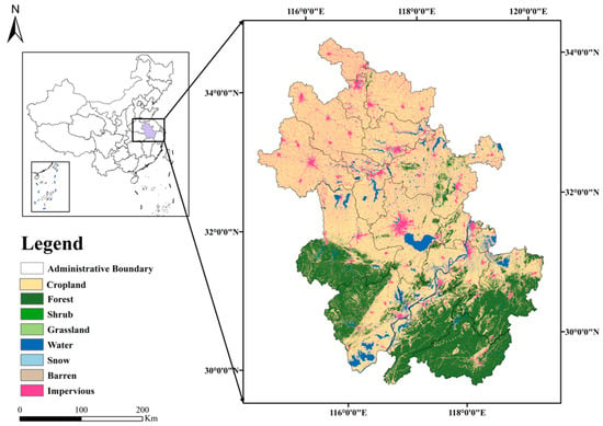
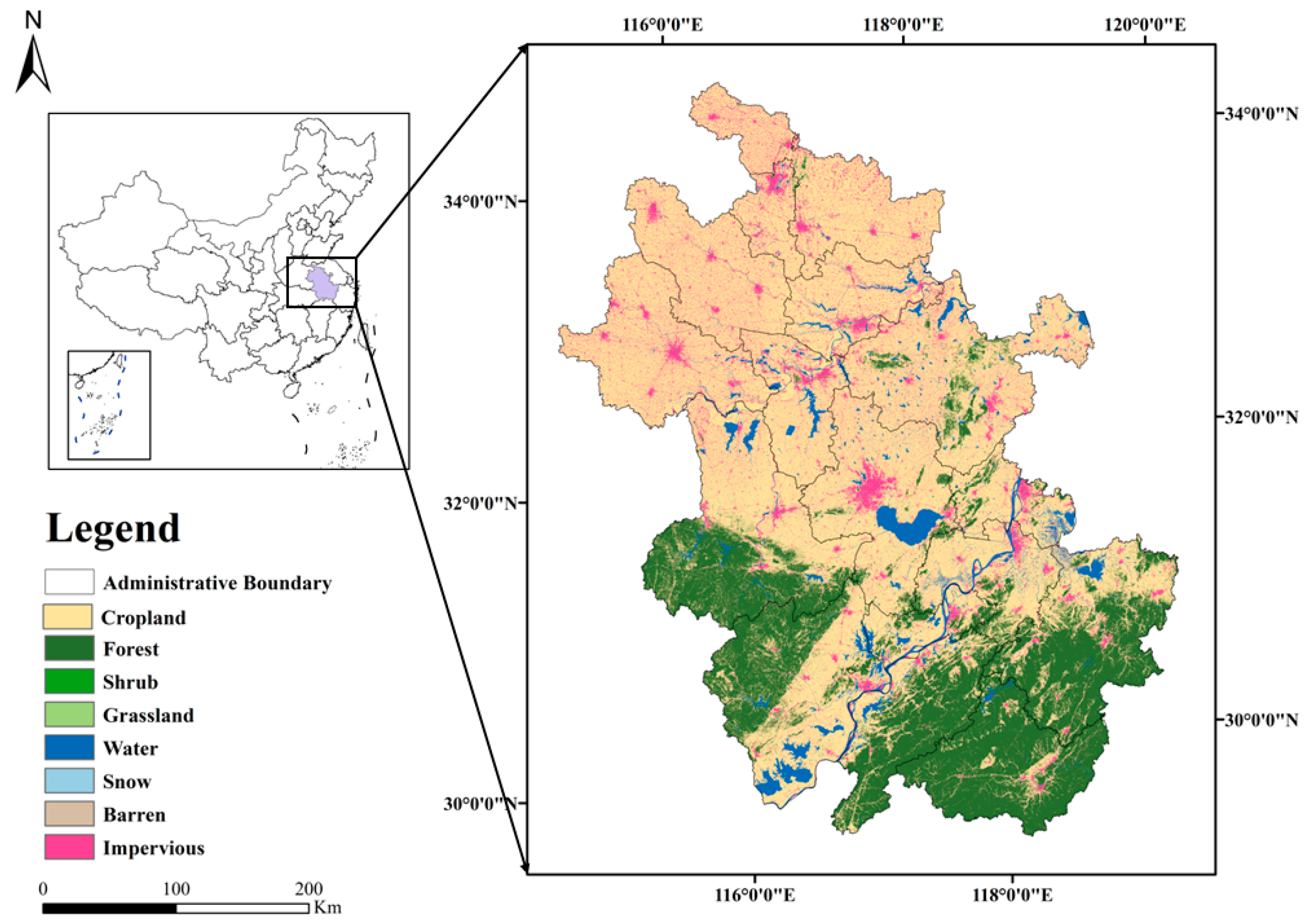
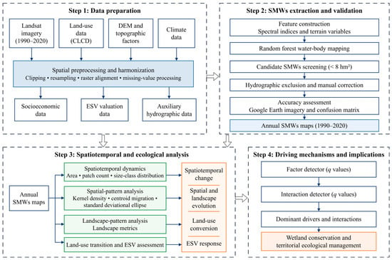
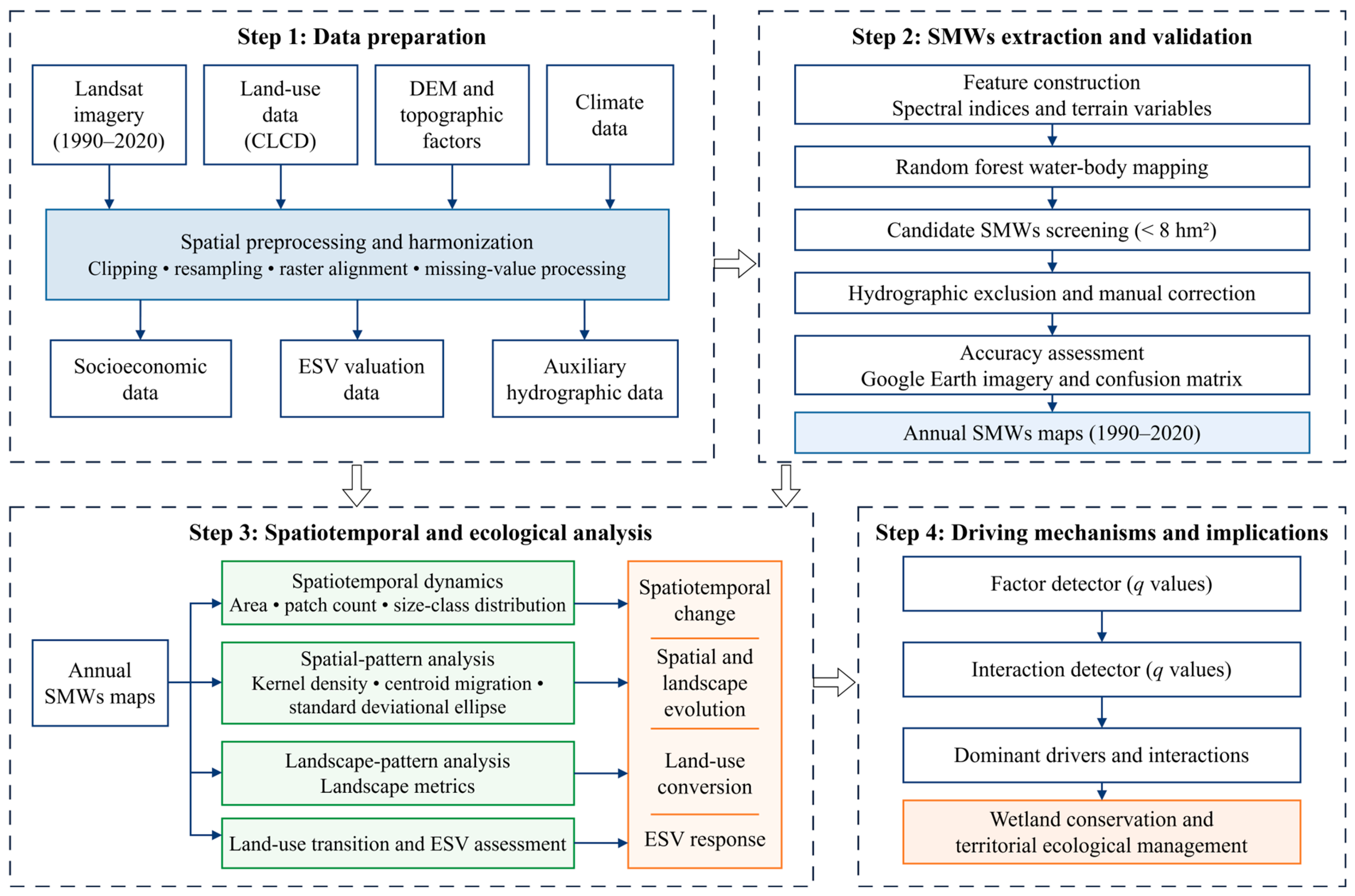
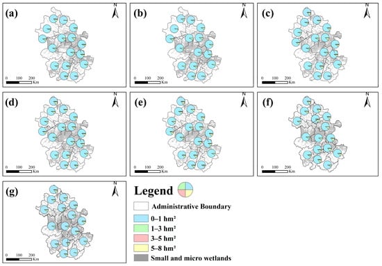
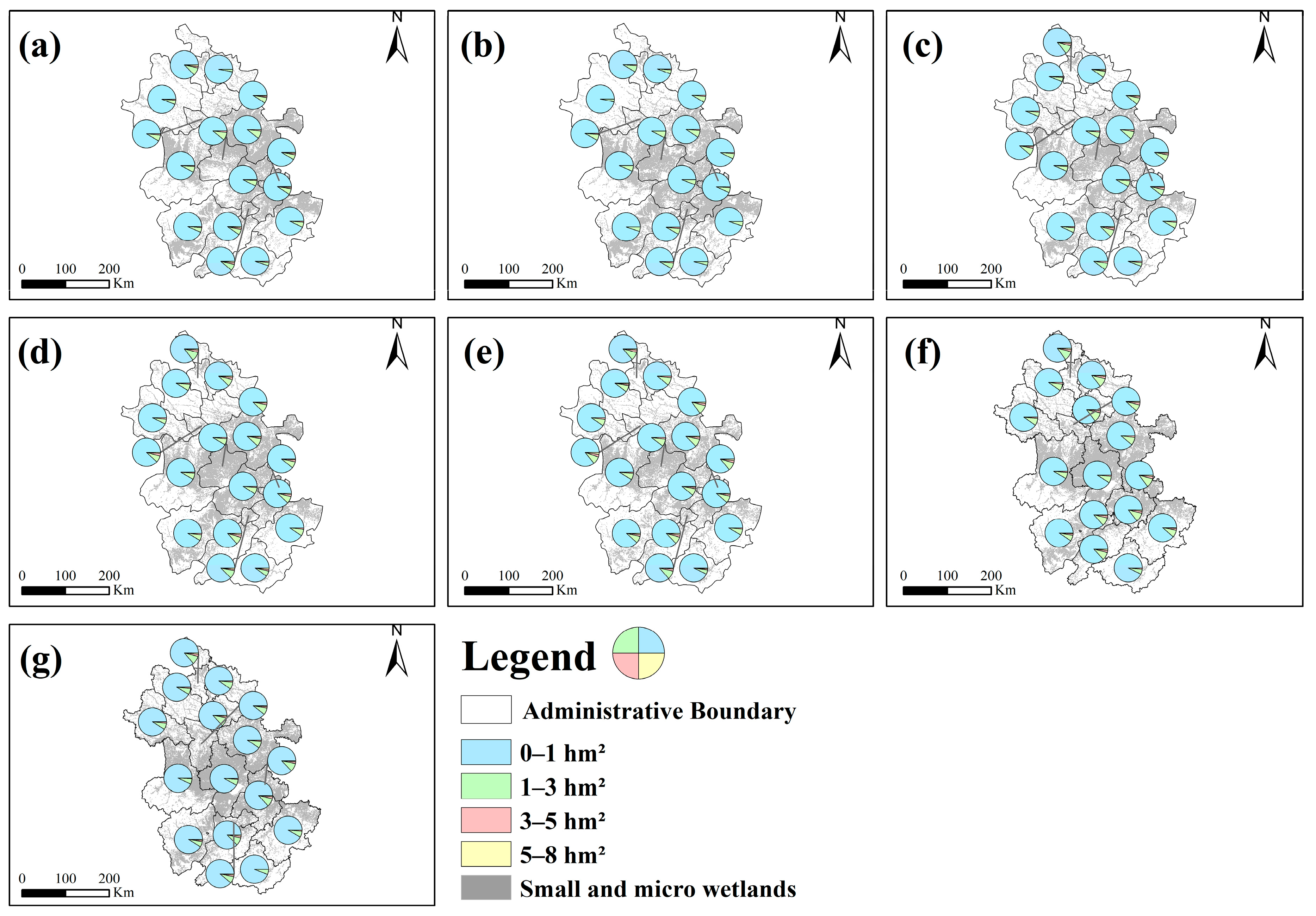
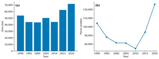
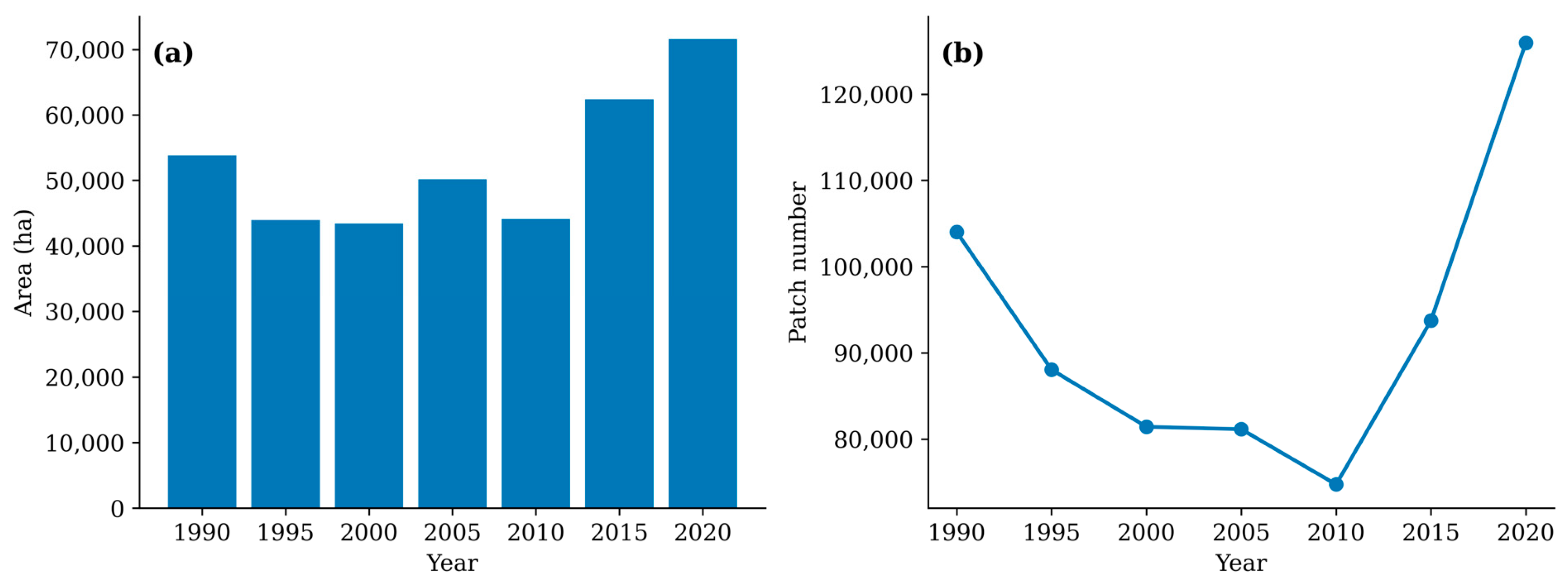
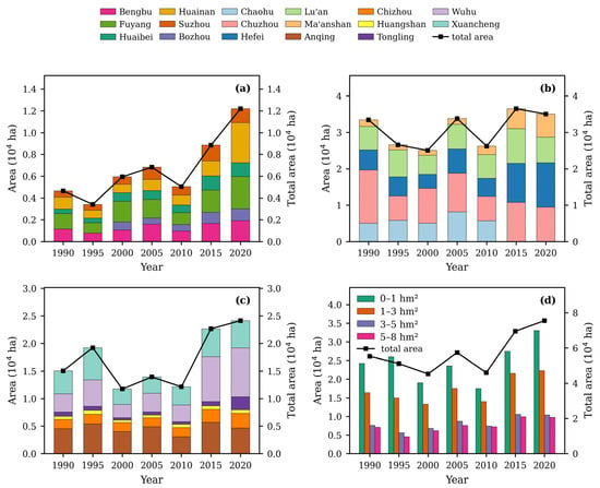
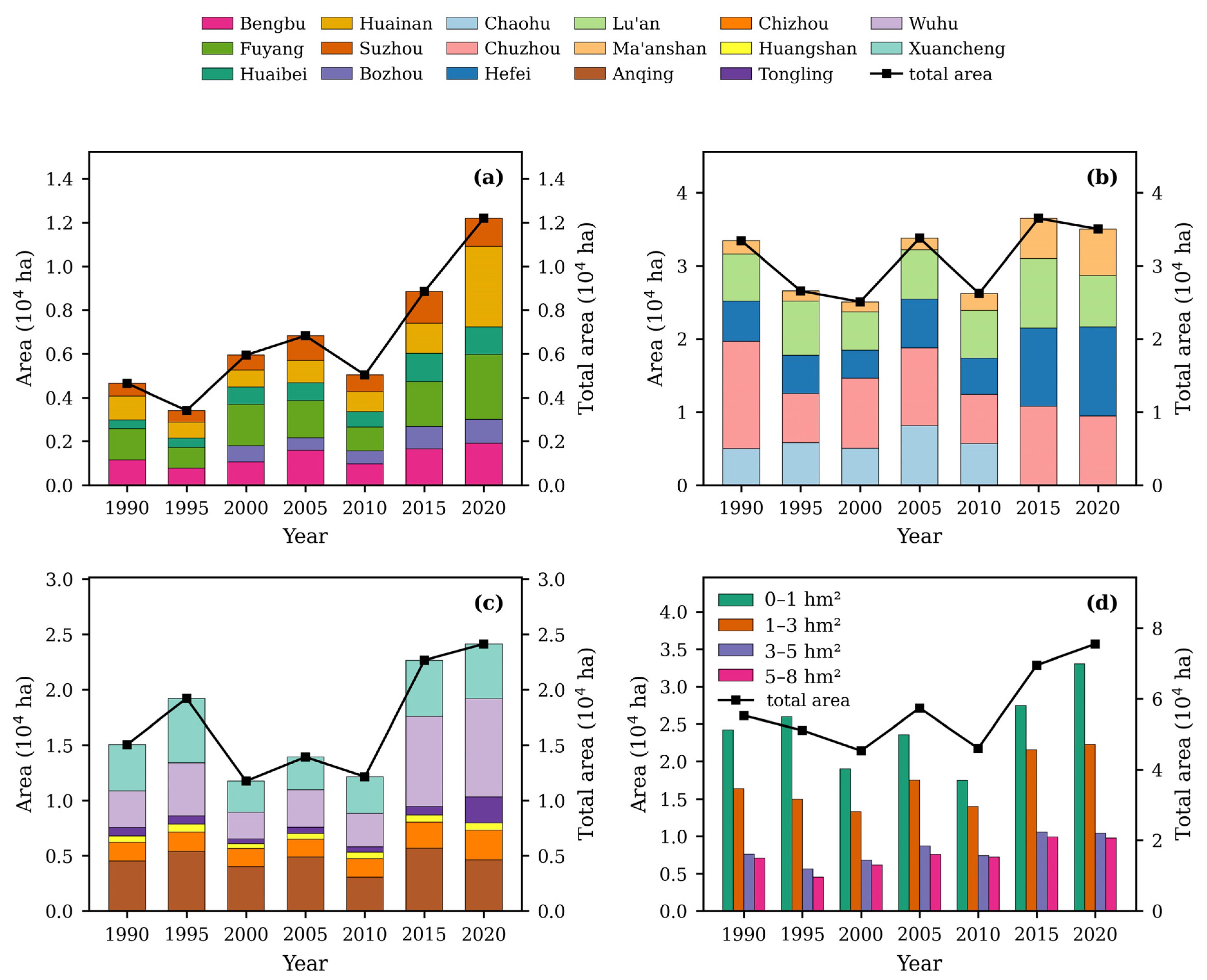
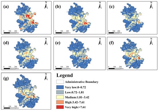
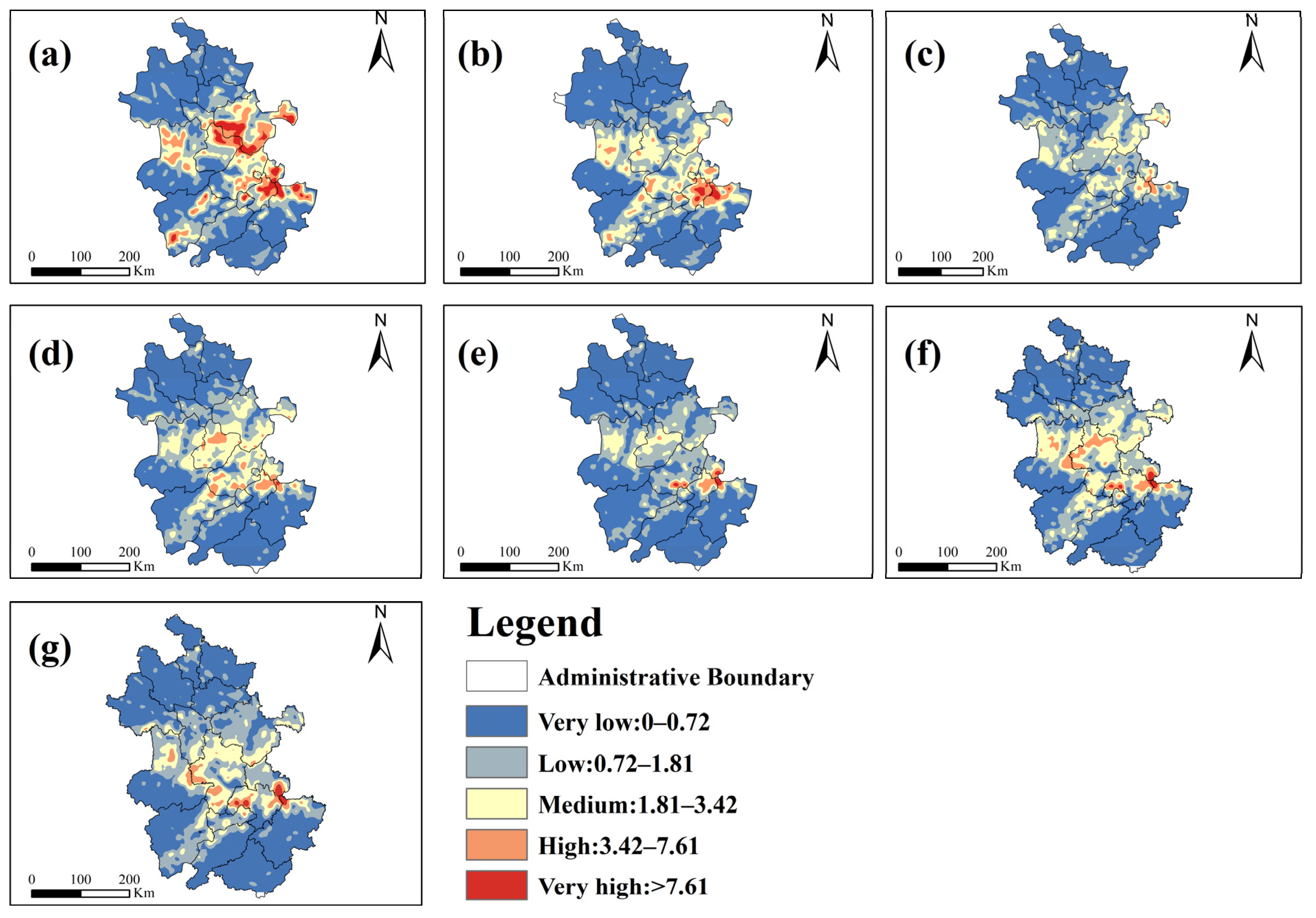
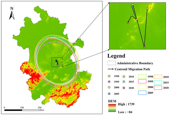
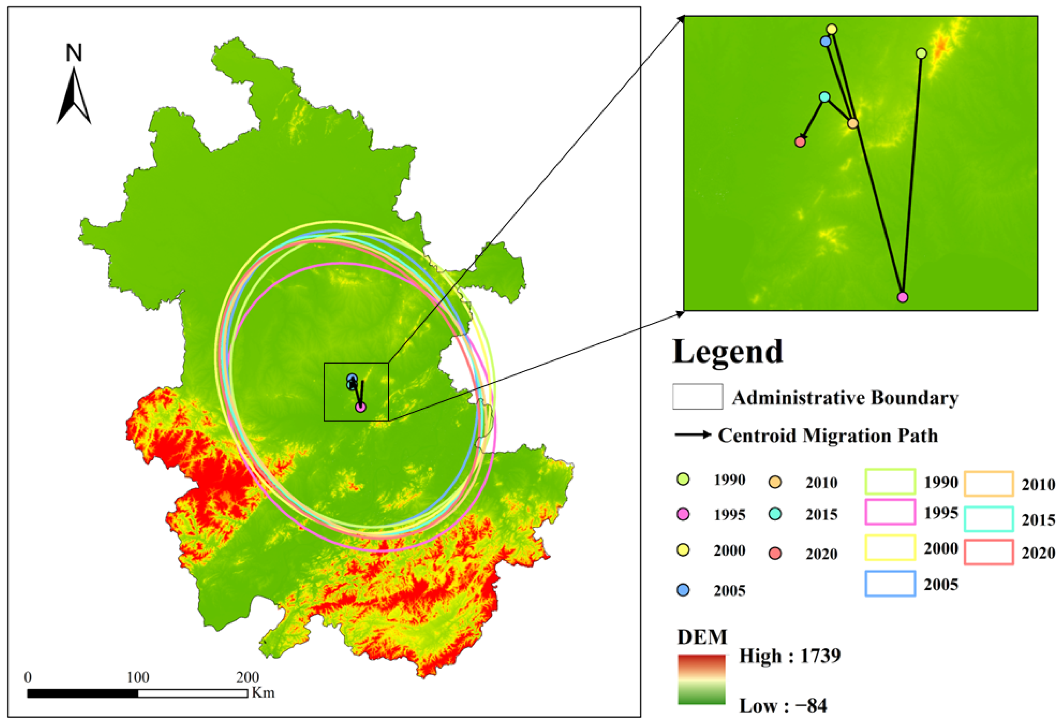
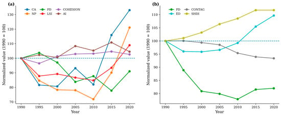
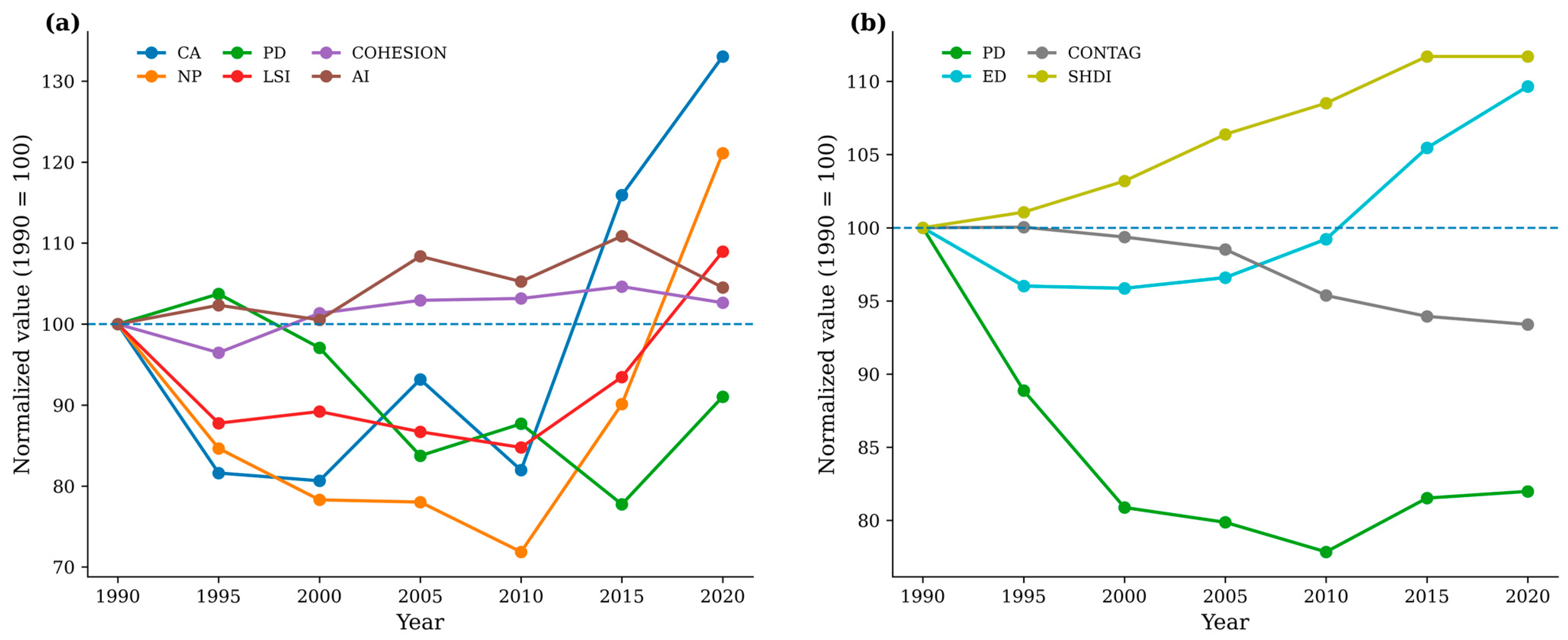
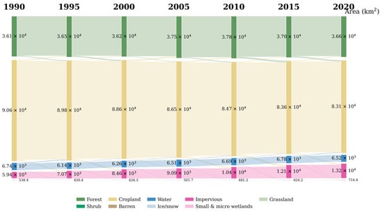
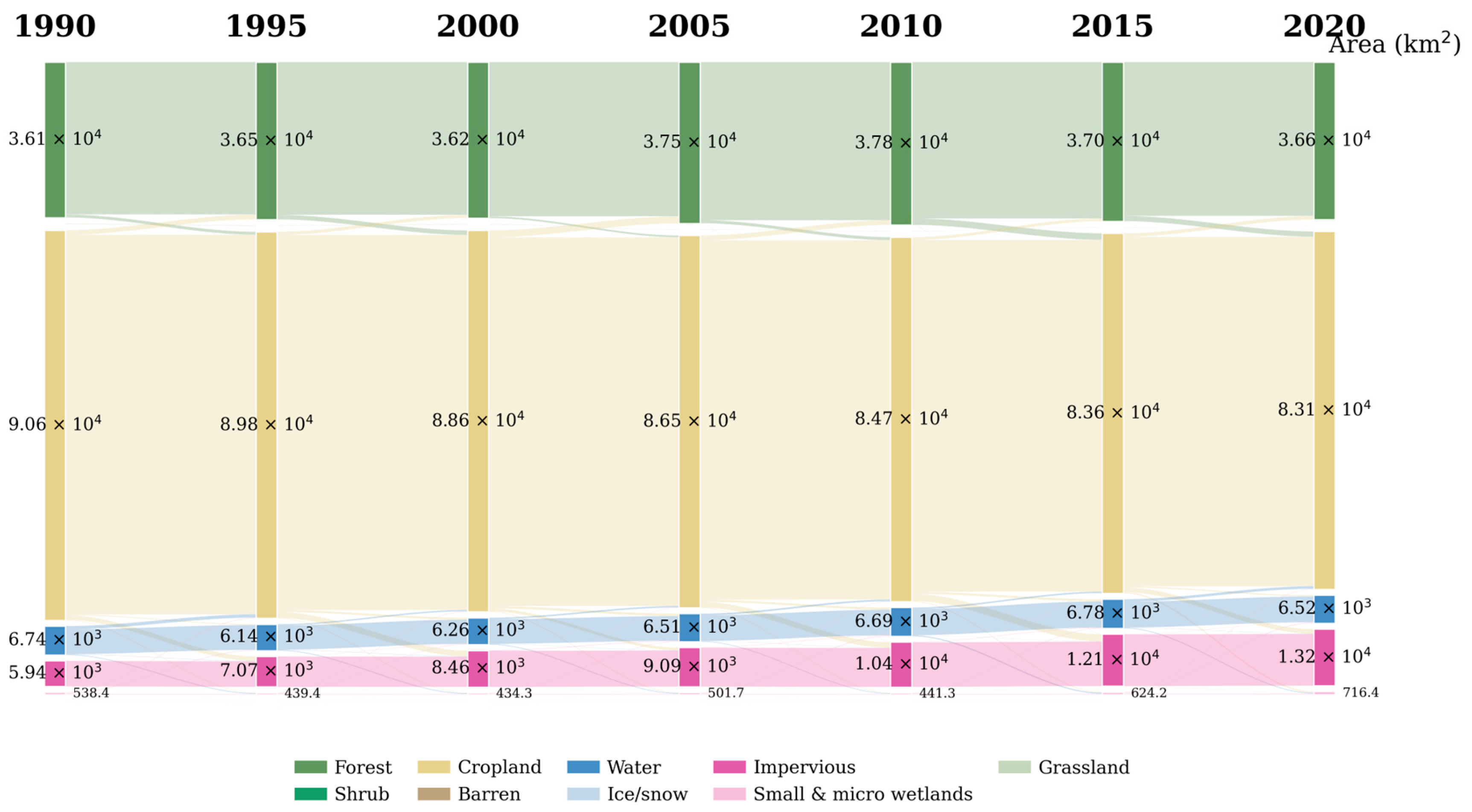
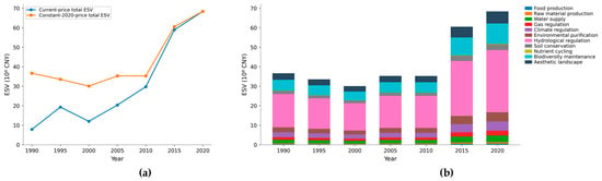
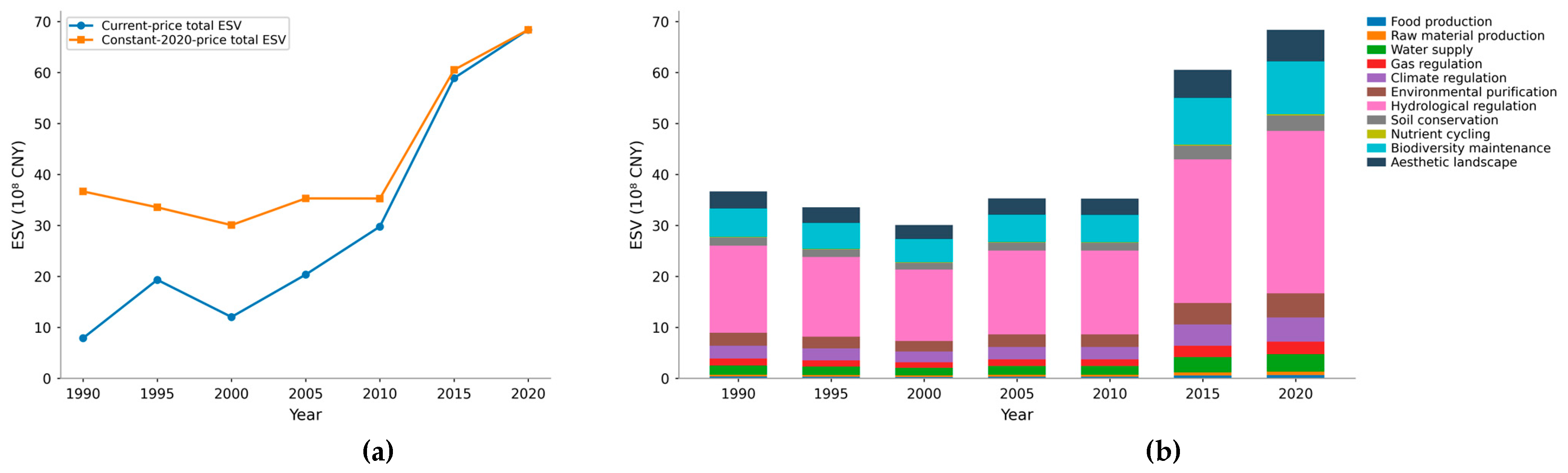
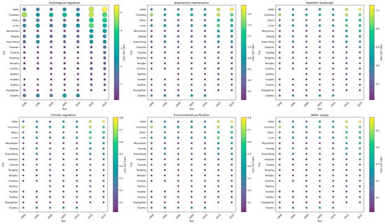
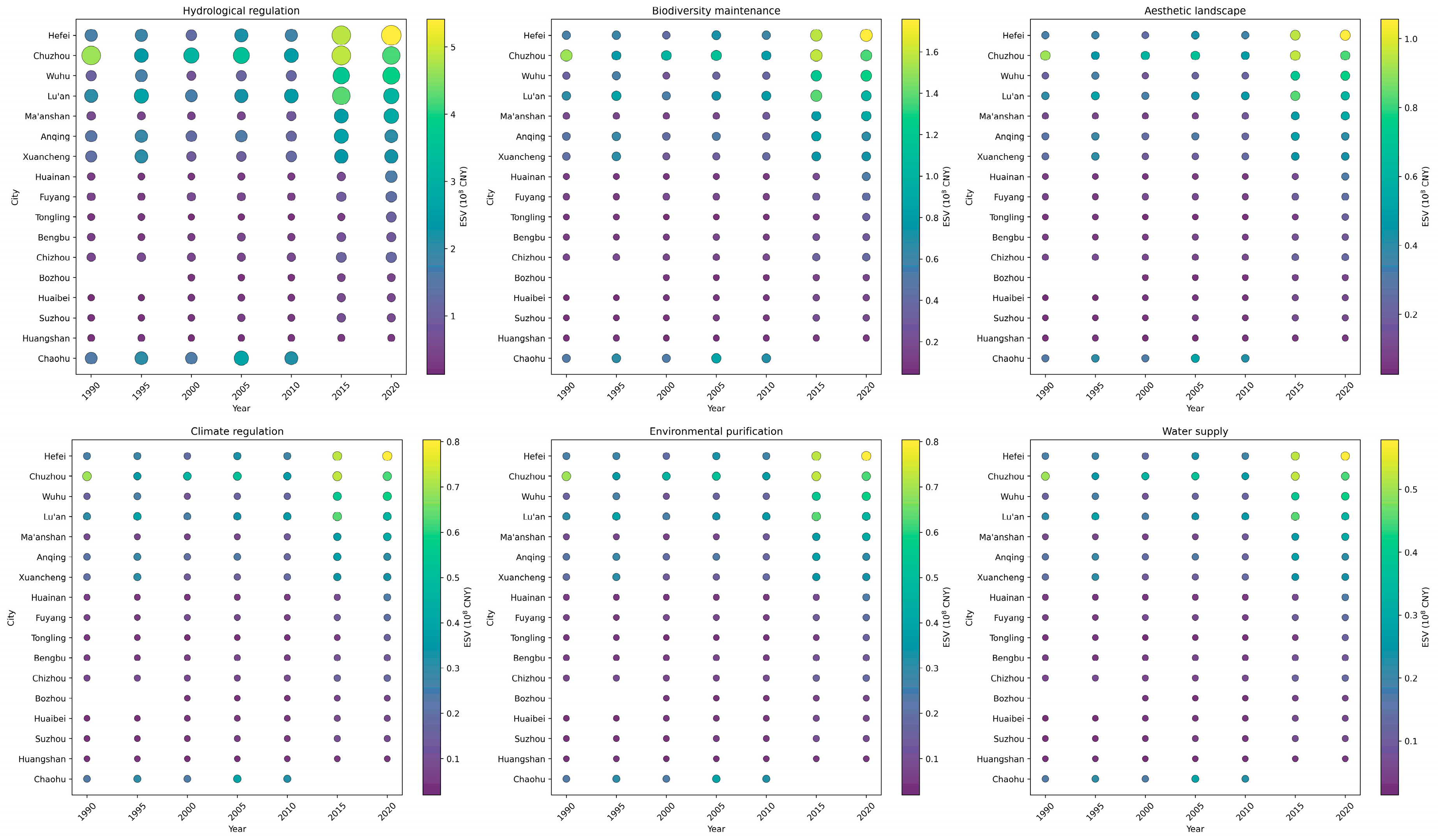
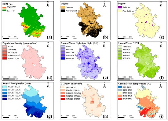
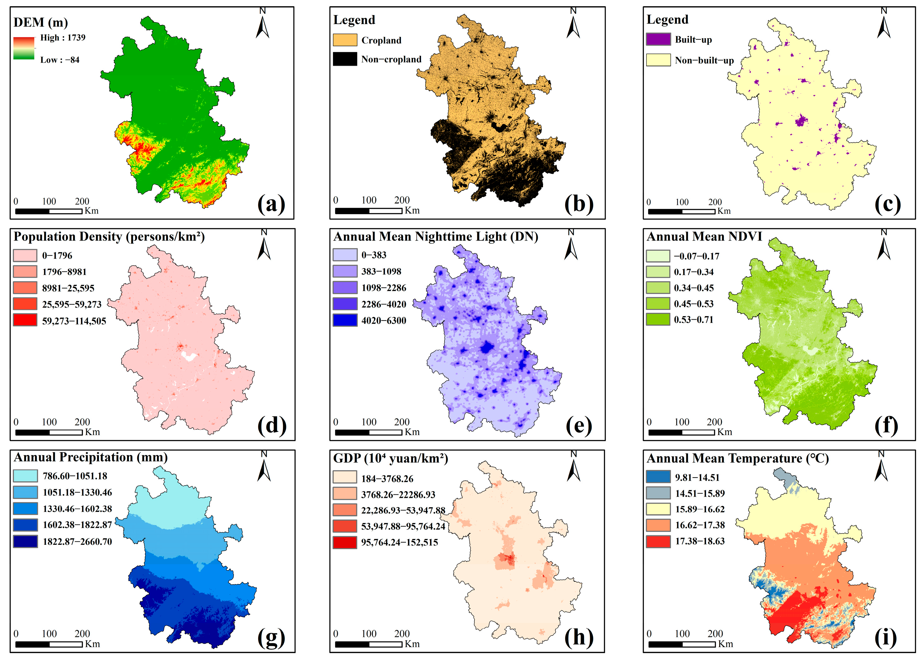
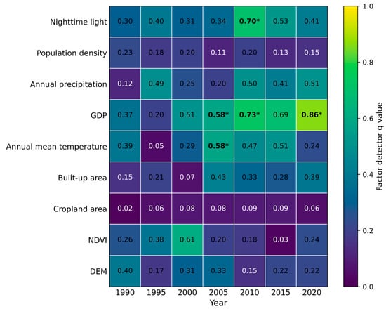
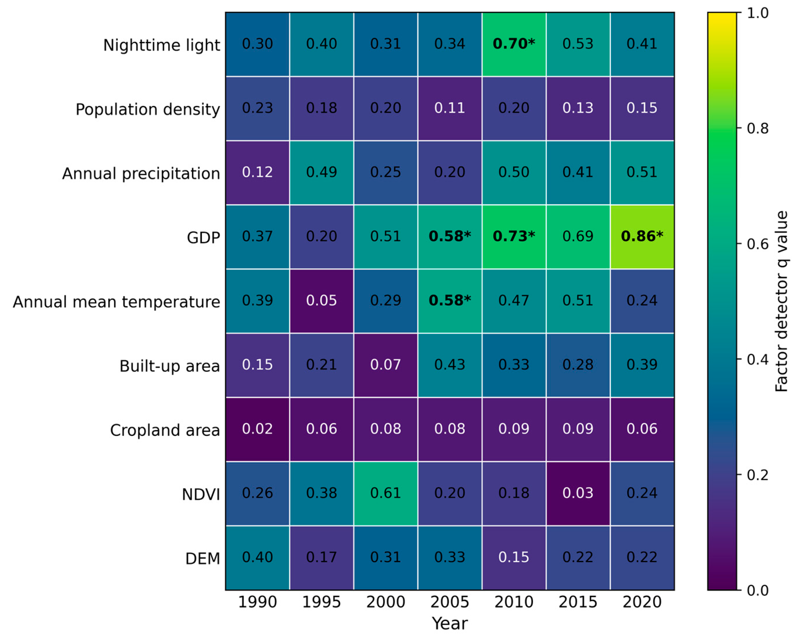
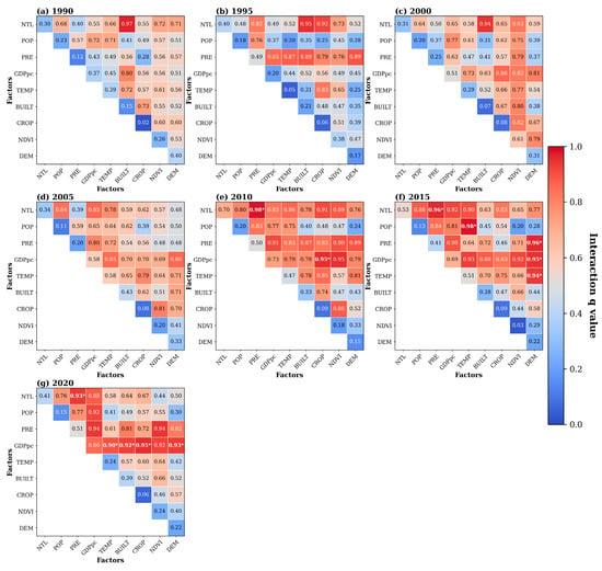
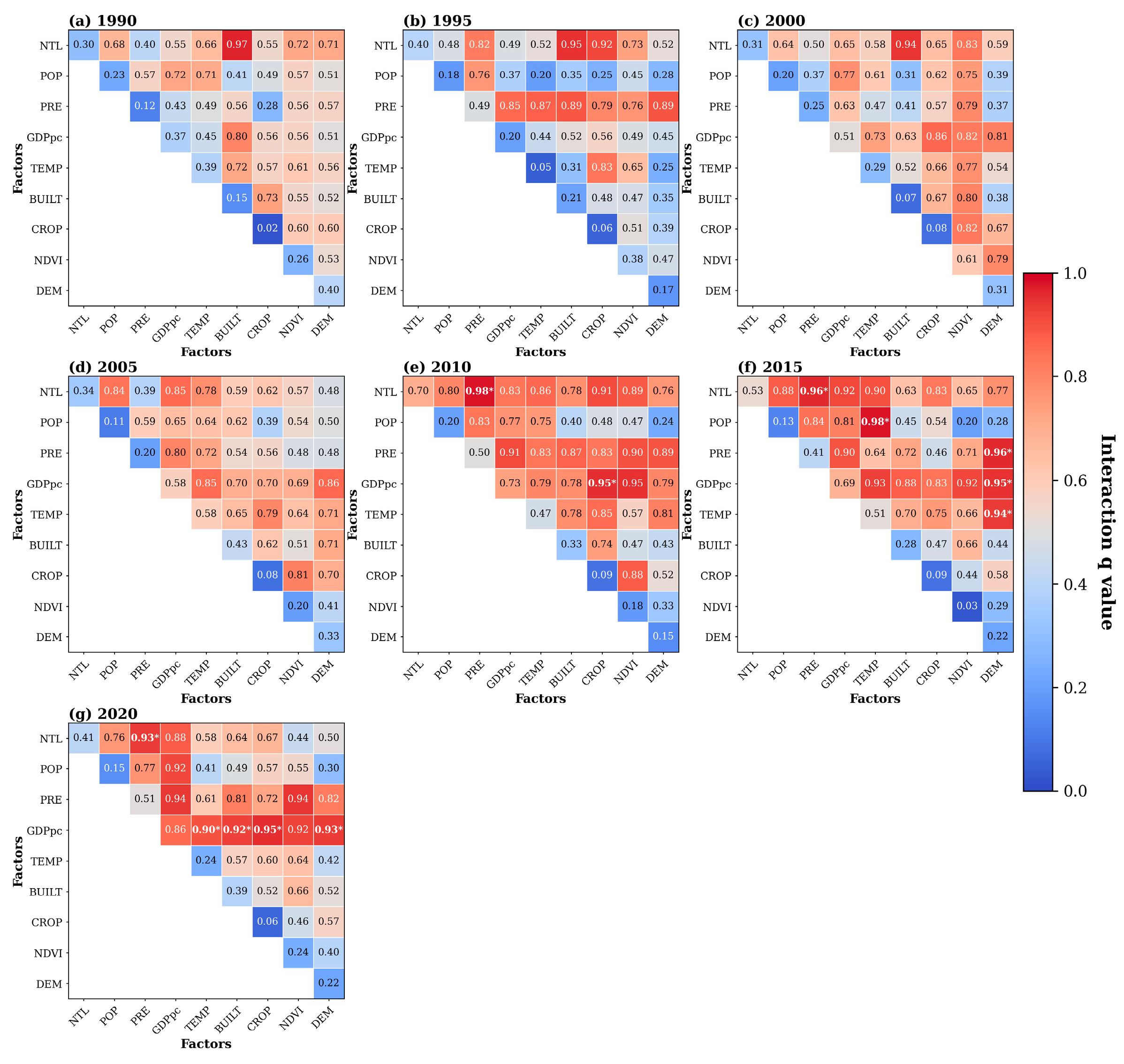

Disclaimer/Publisher’s Note: The statements, opinions and data contained in all publications are solely those of the individual author(s) and contributor(s) and not of MDPI and/or the editor(s). MDPI and/or the editor(s) disclaim responsibility for any injury to people or property resulting from any ideas, methods, instructions or products referred to in the content. |
© 2026 by the authors. Licensee MDPI, Basel, Switzerland. This article is an open access article distributed under the terms and conditions of the Creative Commons Attribution (CC BY) license.