Spectral Proxy Parameter Linking Remote Sensing Reflectance and Inherent Optical Properties in Case-2 Waters

Highlights

What are the main findings?

• The spectral proxy parameter k(λ), linking remote sensing reflectance with inherent optical properties, shows clear wavelength dependence and area to area variability in Baltic Sea Case-2 waters under controlled radiative transfer conditions.
• Area-specific three-coefficient second-order polynomial parameterizations more closely reproduce the regional median k(λ) spectra than a single generalized fit.

What are the implications of the main findings?

• The results demonstrate that k(λ) should not be treated as a universal coefficient in optically complex waters, but as an effective optical scaling parameter whose spectral form depends on the local optical environment and on the adopted radiative transfer conditions.
• The proposed framework provides a regional representation of remote sensing reflectance. The OCP-100 comparison preserves the broad spectral ordering but shows substantial underestimation of absolute R_rs and weak station to station correspondence at 555 and 620 nm; therefore, the parameterization is not interpreted as a station-level predictive model.

Abstract

A spectral proxy parameter linking remote sensing reflectance (R_rs) and inherent optical properties (IOPs) was evaluated for six selected areas of the Baltic Sea. Measured IOPs from the individual optical datasets were used to calculate Morel’s unscaled proxy reflectance, whereas area and wavelength specific median IOPs were used as representative inputs to Monte Carlo radiative transfer simulations. Comparison of the individual proxy estimates with the corresponding area-specific Monte Carlo reference reflectance enabled determination of the spectral proxy parameter k. The results demonstrate a clear wavelength dependence and substantial area to area variability of this parameter. The purpose of the study is not to introduce a new fundamental IOPs–R_rs relationship, but to quantify how the effective scaling coefficient of a widely used proxy relationship varies spectrally and regionally in optically complex Case-2 waters. For each investigated Baltic Sea area, the spectral variability of k was approximated using a three-coefficient second-order polynomial. Area-specific parameterizations provide compact descriptions of the regional median k spectra, while a generalized formulation describes only the pooled central tendency. A radiometric evaluation was performed using 24 in situ OCP-100 spectra from the Gulf of Gdańsk (N = 96 wavelength-level pairs). Predicted and measured R_rs yielded r = 0.680, R² = 0.462, a regression slope of 0.258, a mean bias of −0.00475 sr⁻¹, an RMSE of 0.00590 sr⁻¹, and a MAPE of 62.1%. Within-wavelength correlations were weak at 555 and 620 nm (r = 0.140 and 0.067, respectively). Thus, the regional parameterization preserves broad spectral ordering but underestimates absolute R_rs and does not establish strong station-level predictive skill. The results should be interpreted as a regional, configuration-dependent spectral scaling framework.

1. Introduction

A refined understanding of the wavelength-dependent relationship between remote sensing reflectance (R_rs) and inherent optical properties (IOPs) is essential for improving optical remote sensing in optically complex Case-2 waters. In such environments, the spectral signal is shaped by the combined and highly variable effects of phytoplankton pigments, suspended particles, and colored dissolved organic matter, making the IOPs–R_rs relationship more complex than in open ocean Case-1 waters. Establishing reliable relationships between remote sensing reflectance and the inherent optical properties of natural waters remains a central challenge in ocean optics and aquatic remote sensing [1,2,3,4]. Remote sensing reflectance links the radiative signal emerging from the water surface with the optical characteristics of the water column and therefore plays a fundamental role in the interpretation of ocean-color observations and the retrieval of water quality parameters [5,6,7,8].

The spectral shape of water-leaving reflectance is controlled primarily by absorption and scattering processes occurring within the water column [9]. Early theoretical developments in ocean optics provided the radiative transfer framework describing how light propagates in natural waters and how the upwelling radiance field is related to inherent optical properties such as absorption (a) and backscattering coefficients (b_b) [10,11,12,13]. Subsequent studies introduced semi-analytical and empirical formulations that express R_rs as a function of the ratio between backscattering and absorption, which became the basis of many ocean-color algorithms used nowadays [14,15,16,17,18].

A commonly applied formulation links remote sensing reflectance to inherent optical properties through a proportionality factor describing the angular distribution of the underwater light field [19,20,21]. This factor, often denoted as (f/Q), incorporates the effects of multiple scattering and bidirectional radiative transfer in the water column [22,23,24]. Radiative transfer simulations, including Monte Carlo (MC) modeling, have been widely used to investigate this relationship and to evaluate the accuracy of simplified proxy formulations [25]. Among these approaches, the proxy relationship proposed by Morel and Gentili has proven particularly useful because it provides a physically based method for estimating R_rs from measurable optical properties while maintaining computational efficiency [19,26].

The coefficient k(λ) is conceptually related to the classical f/Q factor, but it is not equivalent to it. In formulations based on b_b/(a + b_b), f/Q describes the angular distribution of the underwater light field and depends on radiance geometry, particle scattering, and the optical properties of the water [19,20,21,22,23,24]. Albert and Mobley [25] likewise expressed subsurface remote sensing reflectance as a function of b_b/(a + b_b) while accounting for solar zenith angle, viewing geometry, and wind speed. In the present study, k(λ) is used as an effective scaling coefficient derived for a fixed set of Monte Carlo conditions. Its value should therefore be interpreted within the radiative transfer conditions adopted here.

Recent advances in ocean optics have demonstrated the growing importance of combining semi-analytical algorithms with numerical radiative transfer approaches for improving the accuracy of remote sensing reflectance modeling [27,28,29,30,31]. Radiative transfer simulations, including Monte Carlo techniques, provide detailed insight into the angular structure of the underwater light field and allow for the assessment of simplifying assumptions commonly used in proxy relationships [22,23,24,25]. These methods have been successfully applied in a wide range of studies, including investigations of light propagation in optically complex waters, evaluation of ocean-color inversion algorithms, and the development of satellite-based products for monitoring marine ecosystems and primary production [32,33,34,35,36]. Furthermore, recent studies emphasize the need to integrate physically based modeling with large-scale observational datasets in order to improve the robustness and transferability of bio-optical algorithms across different marine environments [6,29,31,36].

Although such formulations are broadly applicable, their accuracy strongly depends on the optical characteristics of the investigated water body. In optically complex Case-2 waters, the underwater light field is influenced simultaneously by phytoplankton pigments, suspended mineral particles, and colored dissolved organic matter [27,28,29]. These constituents contribute differently to absorption and scattering processes, producing large spatial and spectral variability in optical properties. As a result, algorithms developed for open ocean Case-1 waters often perform poorly in coastal and inland environments [28,29,30,31]. This limitation highlights the importance of developing regionally adapted parameterizations that reflect the local optical conditions of specific water bodies [37,38].

The Baltic Sea is a typical example of an optically complex Case-2 environment [37,39,40]. Its optical properties are strongly influenced by high concentrations of dissolved organic matter, suspended particles, and pronounced seasonal variability in biological activity [40,41,42]. These factors significantly affect the underwater light field and complicate the relationship between inherent optical properties and remote sensing reflectance [37,39,41]. Consequently, dedicated regional studies are required to improve optical models and retrieval algorithms for these areas [38,39,43].

Our previous study addressed this problem for the Gulf of Gdańsk [44]. That work analyzed 34 optical datasets collected at 17 stations during March–May 2009 and compared Morel’s proxy formulation with Monte Carlo radiative transfer simulations to determine a wavelength-dependent scaling coefficient k [44]. The present study builds on that methodological framework but extends the analysis to 187 optical datasets distributed among six Baltic Sea areas and eight target wavelengths. Thus, the overlap with [44] concerns the Gulf of Gdańsk methodological and data basis, whereas the present contribution focuses on regional and spectral variability across a substantially broader Baltic dataset.

The present study therefore evaluates the wavelength and area dependence of k(λ), compares area-specific quadratic parameterizations with a generalized formulation, and assesses the Gulf of Gdańsk parameterization against available in situ radiometric R_rs. The objective is not to establish a universal IOPs–R_rs equation, but to quantify the spectral and regional variability of the effective proxy coefficient under the controlled radiative-transfer configuration used here [19,25,44].

2. Materials and Methods

2.1. Study Area and Dataset

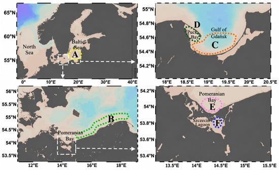
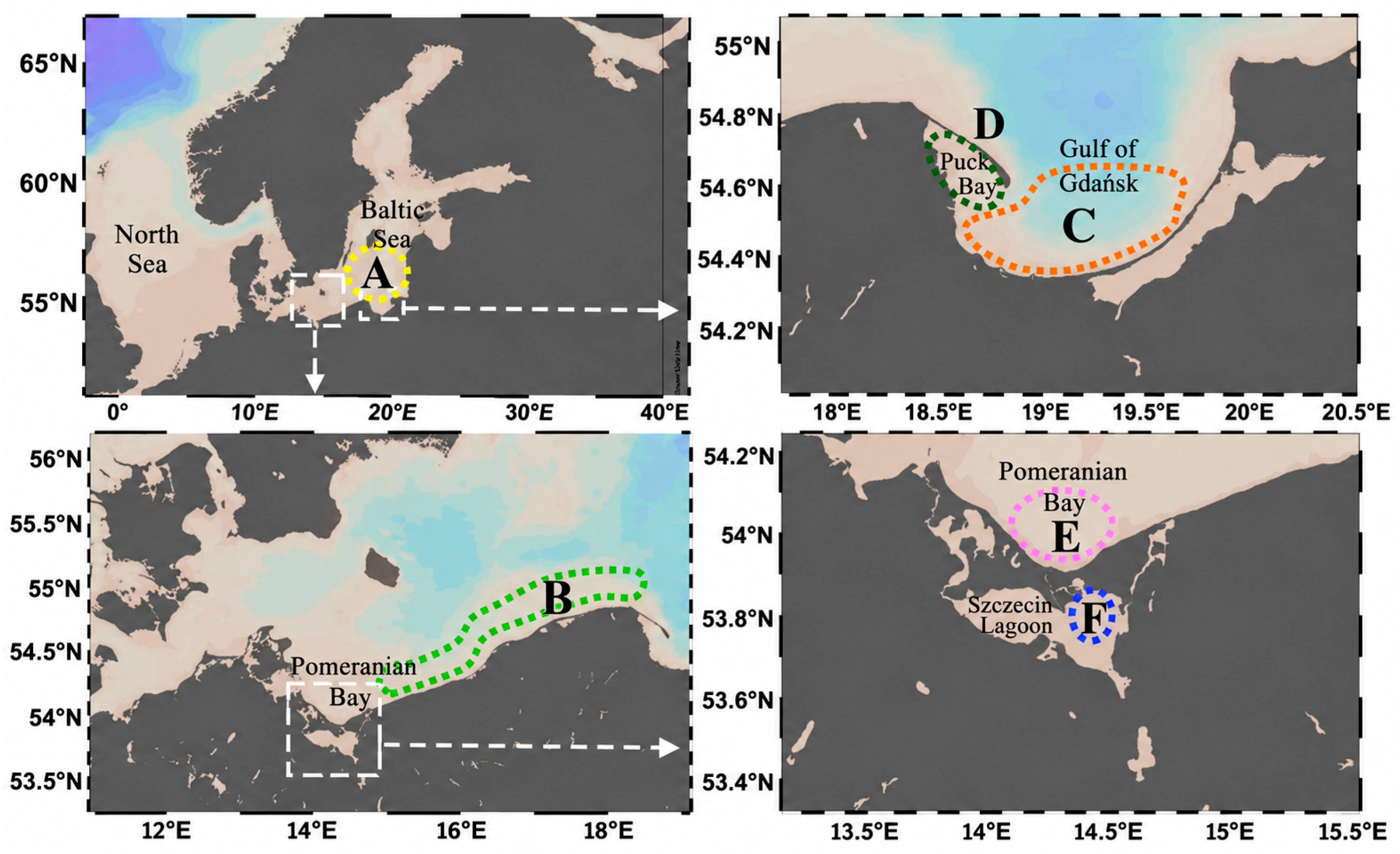
The analysis was conducted for six representative optical areas of the Baltic Sea that exhibit characteristics typical of optically complex Case-2 waters. These areas were selected to span open sea, coastal, gulf, bay, and lagoon environments influenced to different degrees by suspended particles, colored dissolved organic matter (CDOM), and phytoplankton pigments. The dataset was collected during several research cruises between August 2006 and May 2009, providing observations under different seasonal and environmental conditions. The investigated areas include: (A) open waters of the southern Baltic Sea (sBS), (B) coastal waters of the sBS, (C) the Gulf of Gdańsk, (D) Puck Bay, (E) Pomeranian Bay, and (F) the Szczecin Lagoon. The geographical locations of these areas are presented in Figure 1. The sampling effort was not balanced among areas or seasons; therefore, the dataset is used to characterize the range of optical conditions represented by the observations rather than to derive a seasonal climatology.

Figure 1. The locations of Baltic Sea areas for which the spectral proxy parameter was determined. (A) open waters of the southern Baltic Sea (sBS), (B) coastal waters of the sBS, (C) the Gulf of Gdańsk, (D) Puck Bay, (E) Pomeranian Bay, and (F) the Szczecin Lagoon.

In total, the dataset consisted of the following numbers of optical samples for each area: (A) 36 datasets, (B) 20 datasets, (C) 103 datasets, (D) 10 datasets, (E) 12 datasets and (F) 6 datasets. Altogether, these measurements provide a broad representation of optical variability typical of Baltic Sea Case-2 waters. Because areas D–F contain only 6–12 datasets, their regional distributions and constituent statistics are interpreted descriptively.

The unit of analysis is a complete optical dataset rather than a unique station identifier. Each dataset contains the IOP measurements required for the proxy calculation and for construction of the area-specific IOP statistics used as Monte Carlo inputs. Ancillary chlorophyll a, total suspended solids (TSS), particulate organic matter (POM), and particulate inorganic matter (PIM) data were used for optical interpretation. Because the temporal coverage is not balanced among areas, no seasonal or diurnal trends are inferred from the present dataset.

The primary dataset consisted of in situ IOPs measured just below the sea surface, typically at depths of 0.5–1 m. The IOPs sensors were mounted vertically to maintain consistent measurement geometry and to minimize shading and flow disturbances around the instruments. Radiometric observations were not used to derive k(λ) or as inputs to the Monte Carlo simulations. However, archived measurements from an OCP-100 (Satlantic Inc., Victoria, BC, Canada) in-water radiometer were available for a subset of the Gulf of Gdańsk records and were used exclusively for the validation described below.

For 24 Gulf of Gdańsk records from the 2009 cruises, complete radiometric spectra acquired with the OCP-100 were available together with the corresponding IOPs measurements. These radiometric observations were not used in the derivation of k(λ) and therefore provided an observational test of the predicted R_rs. Because the corresponding IOPs measurements belong to area C—Gulf of Gdańsk (Figure 1) and form part of the regional dataset, the validation is not fully independent; nevertheless, the measured R_rs represents an independent radiometric quantity against which the parameterization can be evaluated.

2.2. Measurements of IOPs

The inherent optical properties used in the analysis were derived from in situ measurements obtained with two instruments: an absorption-attenuation meter ac-9 (WET Labs, Philomath, OR, USA) and a spectral backscattering meter Hydroscat-4 (HOBI Labs, Bellevue, Washington, WA, USA). The methodology itself is not instrument-specific: it requires calibrated spectral estimates of absorption/attenuation and backscattering that can also be obtained with equivalent instruments, provided that appropriate temperature, salinity, scattering, and pure-water corrections are applied and that the measurements refer to the same water mass.

The ac-9 instrument was used to measure absorption and attenuation coefficients of seawater constituents (suspended particles and colored dissolved organic matter (CDOM)) at nine wavelengths (412, 440, 488, 510, 532, 555, 650, 676, and 715 nm). The instrument was calibrated prior to each deployment following the manufacturer’s procedures, including dark calibration and reference measurements with filtered Milli-Q water. Measured absorption and attenuation values were corrected for temperature and salinity effects and subsequently adjusted for scattering contributions using established correction procedures [45,46].

The scattering coefficient of suspended constituents b_p(λ) was obtained as the difference between the attenuation and absorption coefficients measured by the ac-9 system.

The Hydroscat-4 sensor provided measurements of the volume scattering function at a scattering angle of 140°. From these measurements, the total backscattering coefficient b_b(λ) was derived at four wavelengths (420, 488, 555, and 620 nm) following standard processing procedures for this instrument [47,48].

The particulate backscattering coefficient b_bp(λ) was then obtained by subtracting the contribution of backscattering by seawater molecules [49] from the total backscattering signal. Measurements from both instruments were acquired simultaneously during each station stop to ensure that all optical parameters corresponded to the same water mass.

2.3. Spectral Interpolation of the b_bp(λ)

Direct measurements of the particle backscattering coefficient were available at four Hydroscat-4 wavelengths: 420, 488, 555, and 620 nm. In order to extend the analysis to the eight target wavelengths required for the ocean-color comparison, the particle backscattering spectrum was reconstructed at the additional wavelengths.

This was achieved using a power-law spectral model, which describes the wavelength dependence of particle backscattering as

b_bp(λ) = X λ^−η

(1)

where X is a proportionality constant and η is the spectral slope parameter.

To estimate the parameters of this relationship, the equation was transformed into logarithmic form:

log(b_bp) = −η log(λ) + Y

(2)

which represents a linear relationship between log(b_bp) and log(λ). Linear regression was then performed using the measured backscattering values at four wavelengths (420, 488, 555, and 620 nm). The regression provided estimates of the spectral slope η and the intercept constant Y. The resulting power-law model was subsequently used to calculate the particle backscattering coefficient at all wavelengths required for the analysis. Using this approach, spectral values of b_bp(λ) were obtained for the eight wavelengths considered in this study: 412, 440, 488, 510, 532, 555, 650, and 676 nm.

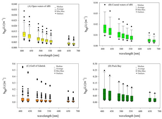
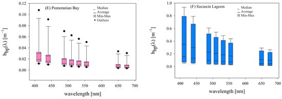
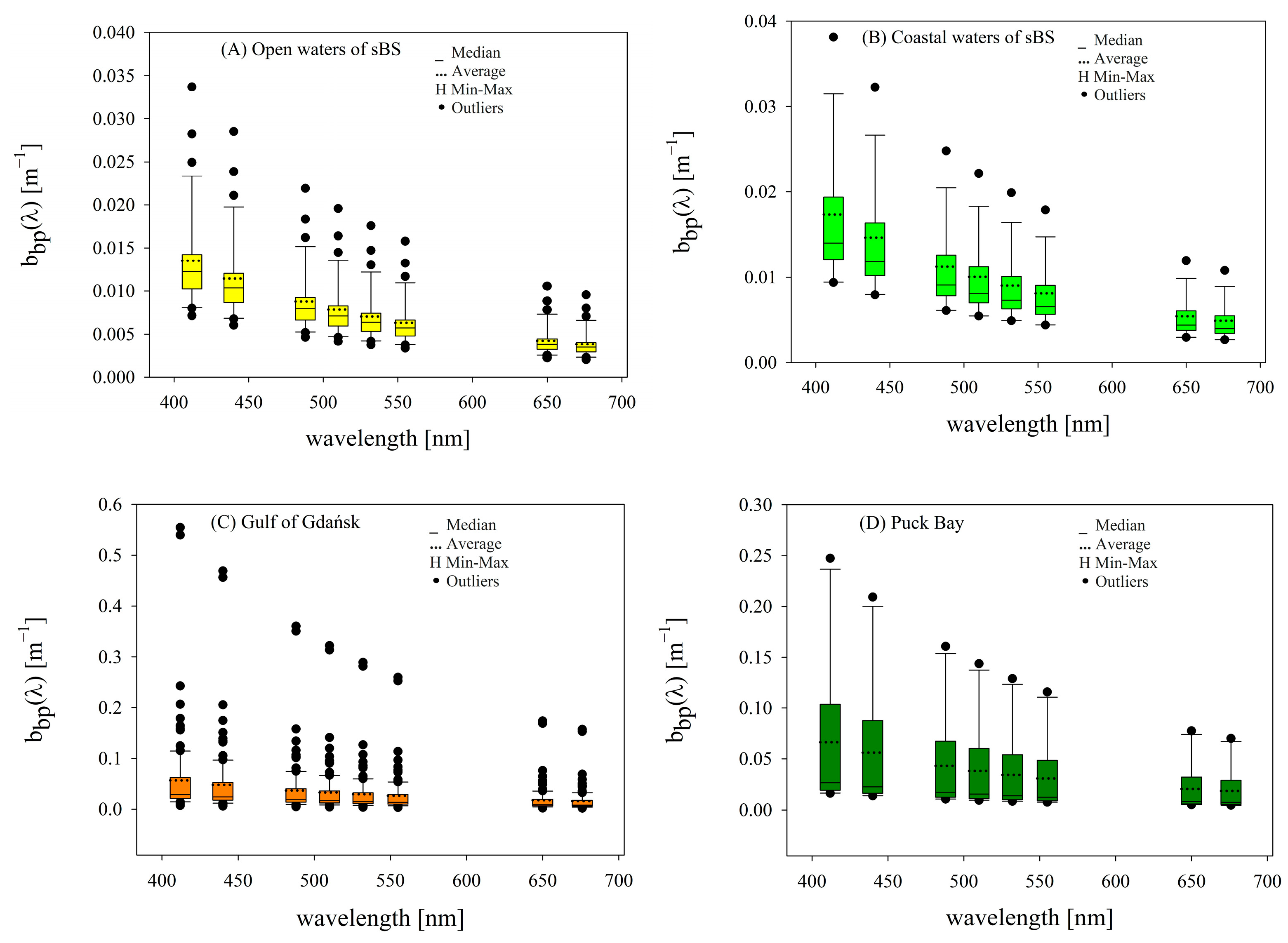
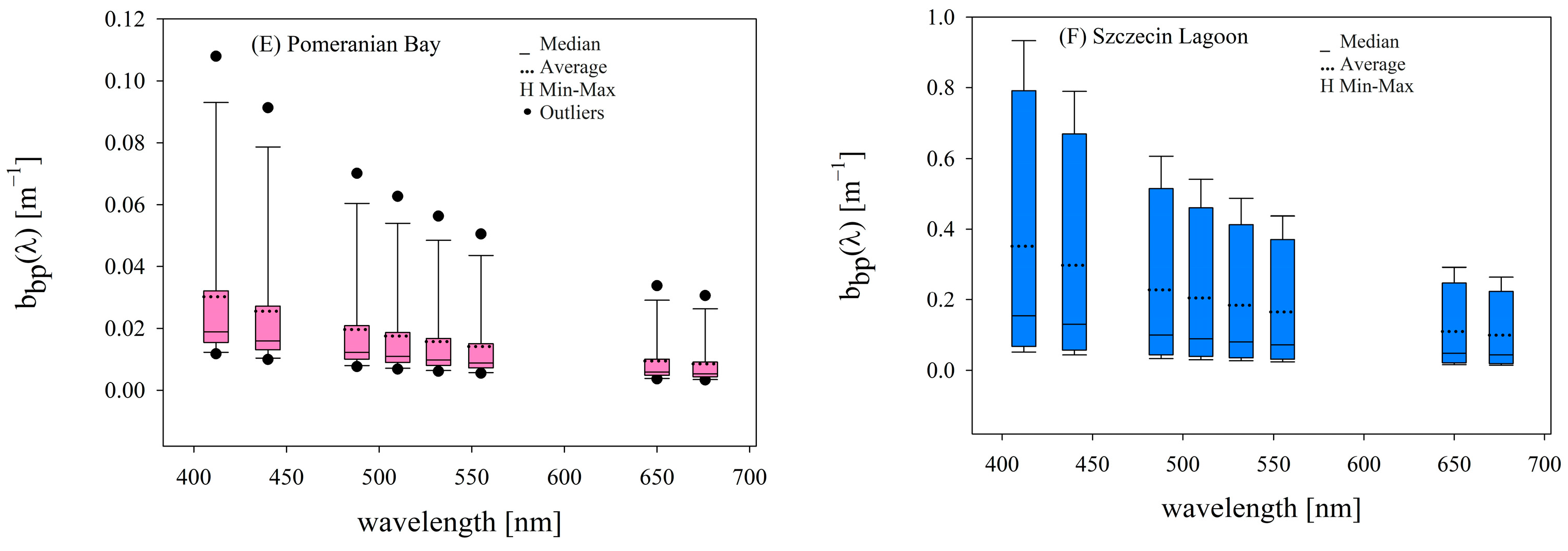
The statistical distributions of the interpolated particle backscattering coefficients for each investigated Baltic Sea area are shown in Figure 2. The results demonstrate clear spectral variability of b_bp(λ) across all analyzed environments. Higher backscattering values are generally observed in optically complex coastal and lagoon waters, particularly in the Szczecin Lagoon and the Gulf of Gdańsk, while lower values occur in the open waters of the southern Baltic Sea. The distributions also show considerable variability within individual areas, reflecting the dynamic optical conditions typical of Case-2 waters. In Figure 2, the whiskers represent the range of non-outlier values (i.e., data within 1.5 times the interquartile range from the first and third quartiles), while values outside this range are displayed as outliers and may correspond to the actual minimum and maximum observations.

Figure 2. The particulate backscattering coefficients b_bp(λ) for selected areas of the Baltic Sea, reconstructed at eight wavelengths: 412, 440, 488, 510, 532, 555, 650, and 676 nm. Sample sizes are: (A) n = 36, (B) n = 20, (C) n = 103, (D) n = 10, (E) n = 12, and (F) n = 6. Vertical bars represent the range of variation, H-shaped whiskers indicate the minimum and maximum values, dashes mark the median, dashed lines denote the mean, and black dots indicate outliers. The rectangles represent the interquartile range (25–75%).

Because the particle backscattering coefficient was directly measured only at four wavelengths, its spectral reconstruction introduces an additional source of uncertainty. The power-law representation was selected because it is a standard spectral form for particulate backscattering in semi-analytical ocean-color approaches and expresses the spectrum through the physically interpretable slope parameter η [13,17]. Fitting the relationship in log–log space uses all four measured Hydroscat-4 bands (420, 488, 555, and 620 nm) and preserves positive b_bp(λ) values over the reconstructed spectrum. Values at 412 nm and in the 650–676 nm range involve short extrapolations beyond the directly measured bands and are therefore explicitly treated as an additional source of uncertainty.

2.4. Determination of Total Optical Properties

The total absorption coefficient of seawater was calculated as

a(λ) = a_pg(λ) + a_w(λ)

(3)

where apg represents absorption by particles and dissolved organic matter and aw denotes absorption by pure water molecules. Values of pure water absorption were taken from the dataset reported by Pope and Fry [50].

The two computational branches used different representations of particle backscattering. In the Morel-type proxy branch, total backscattering was calculated from measured/reconstructed Hydroscat-4 particulate backscattering and the molecular contribution of pure water. In the Monte Carlo branch, measured Hydroscat-4 b_bp was not imposed as an independent input. Instead, measured particulate scattering b_p and the prescribed Petzold coastal water phase function determined the angular redistribution of particle scattering; molecular scattering and backscattering terms followed Morel [49].

For each area and wavelength, the arithmetic mean and median of the measured absorption and particulate scattering coefficients were calculated to characterize the available IOPs distributions. Area-specific median a(λ) and b_p(λ) values were selected as representative Monte Carlo inputs because the Case-2 distributions are frequently skewed and may contain episodic extremes. Measured Hydroscat-4 b_bp values were not included among the Monte Carlo inputs.

Importantly, the statistical reduction to median IOPs was applied only to the Monte Carlo branch of the analysis. Morel’s unscaled proxy reflectance was calculated separately for each individual optical dataset using the measured/reconstructed b_b(λ) and the corresponding absorption coefficient; the proxy calculations were therefore not performed from area-averaged or median IOPs.

For each area r and individual dataset i, the spectral proxy parameter was obtained by pairing the individual proxy estimate R_{rs_un,r,i}(λ) with the Monte Carlo reference reflectance R_{rs_MC,r}(λ) calculated for the median optical state of that area. Thus, k_r,i(λ) = R_{rs_MC,r}(λ)/R_{rs_un,r,i}(λ). Individual k values are scaling quantities referenced to a representative regional Monte Carlo state, not independently simulated station-specific radiative transfer coefficients. The area-level median k values were subsequently used to derive the spectral parameterizations.

The adopted design comprised 48 Monte Carlo simulations (six areas × eight wavelengths), each representing an area-specific median optical state and propagating approximately two billion photon histories. A fully dataset specific evaluation would require 1496 simulations (187 datasets × 8 wavelengths) and was not performed. Accordingly, the Monte Carlo component is used as a controlled regional reference, and no station-level model skill claim is made from the internal parameterization comparison.

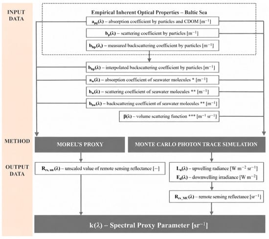
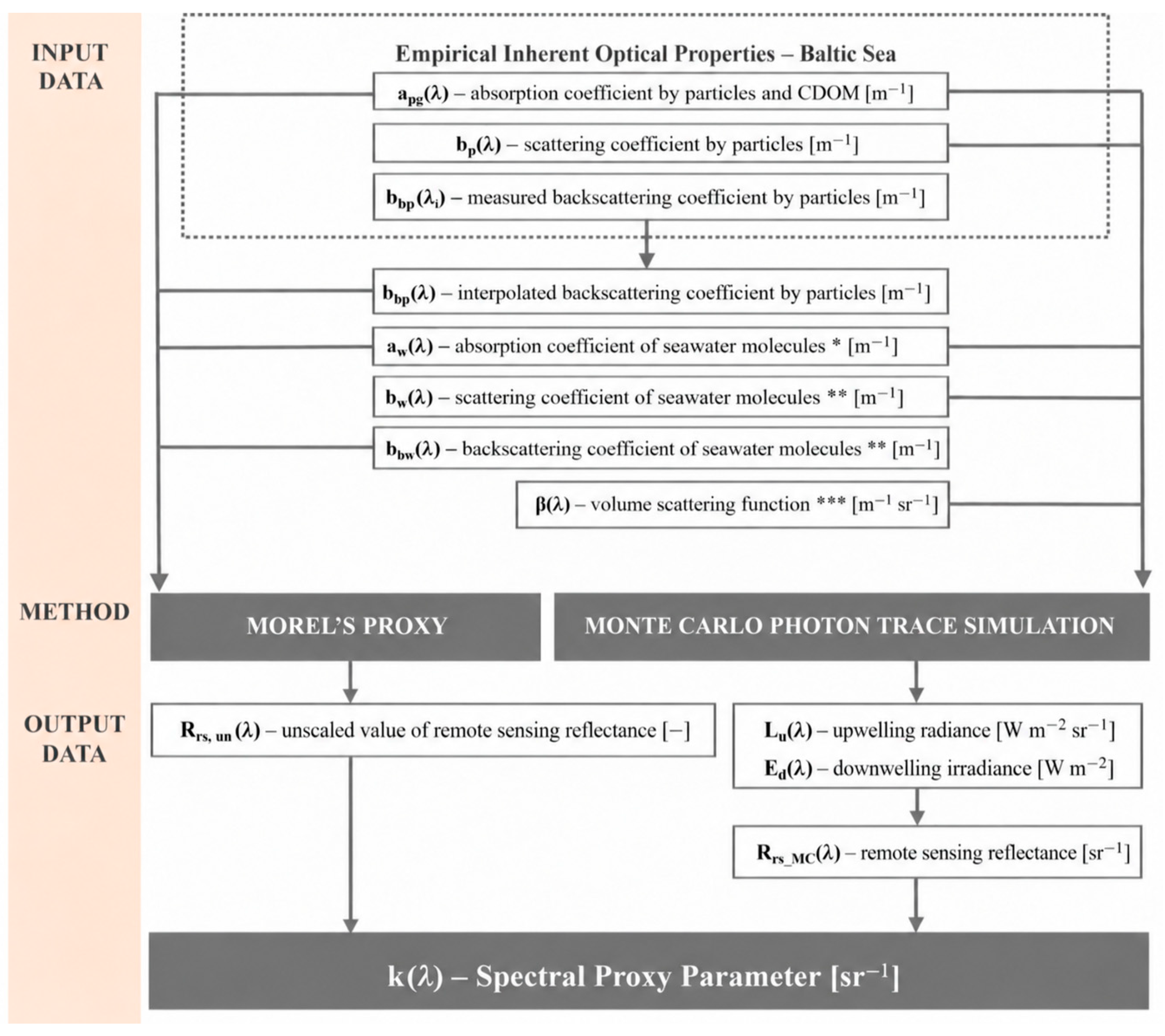
A schematic representation of the entire computational procedure, including input data, modeling methods, and output parameters, is presented in Figure 3.

Figure 3. Block diagram of the determination of the spectral proxy parameter using Morel’s proxy formulation and Monte Carlo simulation for selected Baltic Sea areas at λ = 412, 440, 488, 510, 532, 555, 650, and 676 nm. The proxy branch uses measured absorption and Hydroscat-4 particulate backscattering, with b_bp(λ) reconstructed from the four directly measured bands λ_i = 420, 488, 555, and 620 nm. The Monte Carlo branch uses area and wavelength specific median absorption and particulate scattering derived from ac-9 measurements; measured Hydroscat-4 b_bp is not an input to the Monte Carlo calculation. Particle angular scattering is represented by the same Petzold coastal-water phase function in all six areas. * according to Pope and Fry [50], ** according to Morel [49], and *** according to Petzold [51].

2.5. Monte Carlo Radiative Transfer Simulations

Remote sensing reflectance was calculated using a Monte Carlo photon-tracking radiative transfer model. In this approach, photons were propagated through the simulated water column and their interactions with absorbing and scattering constituents were treated probabilistically according to the specified inherent optical properties.

The Petzold coastal water phase function β(λ) was adopted to represent particle angular scattering in all Monte Carlo simulations [51]. The same phase function was used for each area to maintain a common angular scattering assumption while the measured regional absorption and particulate scattering inputs varied. Because measured Hydroscat-4 b_bp was not imposed in the Monte Carlo branch, particle backscattering in that branch is determined by b_p together with the adopted phase function. The resulting k(λ) therefore includes the consequences of this phase function-based representation and should not be interpreted as a geometry independent f/Q factor.

Surface boundary conditions were modeled using the Cox–Munk statistical representation of a wind roughened sea surface at a fixed wind speed of 5 m s⁻¹ [52]. The sky radiance distribution was generated with RADTRAN under clear sky conditions [53] and a fixed solar zenith angle of 30°, and the lower boundary was treated as optically deep. The 30° solar zenith angle is a controlled reference geometry used consistently in the simulations; it is not intended to reproduce the actual March–May solar geometry at 54–55°N. This fixed configuration provides a common basis for comparison among optically heterogeneous Baltic waters [54].

For each simulation, the trajectories of approximately two billion virtual photons were tracked to ensure numerical stability of the computed radiance fields.

Virtual detectors positioned just below the water surface recorded the modeled upwelling radiance L_u(0⁻) and downwelling irradiance E_d(0⁻). No field radiometric L_u or E_d observations were used in this calculation. The modeled subsurface remote sensing reflectance, denoted here as R_rs__MC(λ), was calculated as

$${\mathrm{R}}_{{\mathrm{rs}}_{\mathrm{MC}}}\left(\mathsf{\lambda }\right)={\displaystyle \frac{{\mathrm{L}}_{\mathrm{u}}\left(0^{-}\right)}{{\mathrm{E}}_{\mathrm{d}}\left(0^{-}\right)}}\hspace{1em}\hspace{1em}\left[{\mathrm{sr}}^{-1}\right]$$

(4)

2.6. Proxy Estimation of Remote Sensing Reflectance

In addition to the Monte Carlo simulations, the proxy formulation was evaluated for every individual optical dataset using the measured inherent optical properties of that dataset. No area averaging was applied before this calculation. The unscaled proxy reflectance was computed as

$${\mathrm{R}}_{\mathrm{rs}\_\mathrm{un}}\left(\mathsf{\lambda }\right)={\displaystyle \frac{{\mathrm{b}}_{\mathrm{b}}\left(\mathsf{\lambda }\right)}{\left(\mathrm{a}\left(\mathsf{\lambda }\right)+{\mathrm{b}}_{\mathrm{b}}\left(\mathsf{\lambda }\right)\right)}}\hspace{1em}\left[-\right]$$

(5)

This formulation is dimensionless and provides an unscaled estimate based solely on the ratio of backscattering to the sum of absorption and backscattering.

2.7. Determination of the Spectral Proxy Parameter

To relate the dimensionless proxy formulation to the radiative transfer reflectance solution, a spectral proxy parameter k(λ) was introduced [19]:

$${\mathrm{R}}_{\mathrm{rs}}\left(\mathsf{\lambda }\right)=\mathrm{k}\left(\mathsf{\lambda }\right){\displaystyle \frac{{\mathrm{b}}_{\mathrm{b}}\left(\mathsf{\lambda }\right)}{\left(\mathrm{a}\left(\mathsf{\lambda }\right)+{\mathrm{b}}_{\mathrm{b}}\left(\mathsf{\lambda }\right)\right)}}\hspace{1em}\hspace{1em}\left[{\mathrm{sr}}^{-1}\right]$$

(6)

Because the ratio b_b(λ)/(a(λ) + b_b(λ)) is dimensionless, k(λ) carries the units of sr⁻¹ and supplies the radiometric scaling required for R_rs(λ). The value of k(λ) was determined by comparing the area-specific Monte Carlo reference reflectance with the individual unscaled proxy reflectance:

$$\mathrm{k}\left(\mathsf{\lambda }\right)={\displaystyle \frac{{\mathrm{R}}_{\mathrm{rs}\_\mathrm{MC}}\left(\mathsf{\lambda }\right)}{{\mathrm{R}}_{\mathrm{rs}\_\mathrm{un}}\left(\mathsf{\lambda }\right)}} \left[{\mathrm{sr}}^{-1}\right]$$

(7)

Albert and Mobley [25] developed a forward formulation of subsurface remote sensing reflectance based on b_b/(a + b_b) and radiative transfer simulations that explicitly accounted for solar zenith angle, viewing angle, and wind speed. The present approach has a more limited objective: k(λ) quantifies the spectral scaling required for the Morel-type proxy to match the Monte Carlo reflectance calculated for representative Baltic optical conditions.

3. Results

The spectral proxy parameter k(λ) was calculated for the individual optical datasets by combining each measured data proxy estimate with the corresponding area-specific Monte Carlo reference solution. The resulting distributions show a systematic dependence on wavelength and substantial area to area variability in Baltic Sea Case-2 waters.

3.1. Spectral Variability of the Proxy Parameter

The values of k(λ) for the six study areas are summarized in Table 1.

Table 1. Median values of the effective spectral proxy coefficient k derived from individual optical datasets within each Baltic Sea area at eight wavelengths. Row G is the wavelength-by-wavelength median of the six area-level median values.

Area/Regional Median k [sr−1]	412 nm	440 nm	488 nm	510 nm	532 nm	555 nm	650 nm	676 nm
(A) Open waters of sBS	0.029	0.033	0.047	0.057	0.065	0.068	0.072	0.074
(B) Coastal waters of sBS	0.033	0.039	0.053	0.061	0.069	0.074	0.076	0.075
(C) Gulf of Gdańsk	0.044	0.053	0.077	0.091	0.103	0.117	0.135	0.131
(D) Puck Bay	0.053	0.065	0.094	0.110	0.128	0.147	0.179	0.173
(E) Pomeranian Bay	0.033	0.038	0.061	0.076	0.090	0.099	0.088	0.081
(F) Szczecin Lagoon	0.013	0.018	0.027	0.033	0.039	0.047	0.066	0.066
(G) Median of six area medians	0.033	0.038	0.057	0.069	0.080	0.086	0.082	0.078

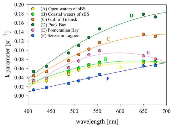
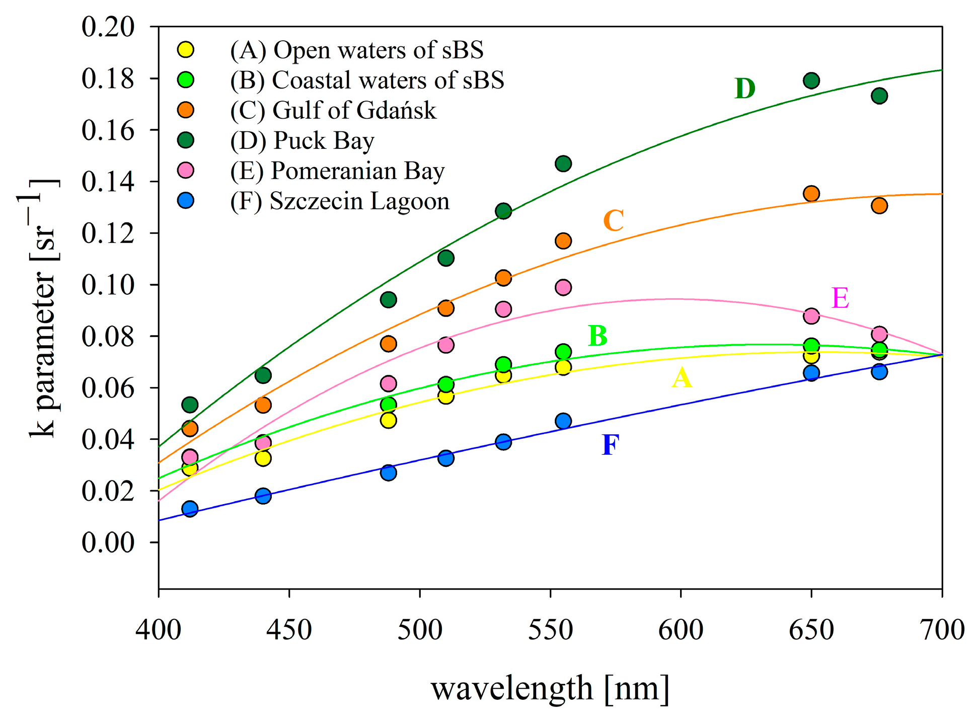
Across all areas, the spectral parameter k(λ) increases from the blue to the red spectral region, with the most pronounced growth observed between 412 nm and approximately 650 nm. In the open waters of the southern Baltic Sea (area A), k(λ) rises from 0.029 sr⁻¹ at 412 nm to 0.074 sr⁻¹ at 676 nm, indicating relatively low variability and overall low magnitude. A similar but slightly enhanced trend is observed in coastal waters (area B), where values range from 0.033 sr⁻¹ to approximately 0.075–0.076 sr⁻¹ at the longest wavelengths.

More optically complex environments exhibit substantially higher values of the proxy parameter in some areas. In the Gulf of Gdańsk (area C), k(λ) increases from 0.044 sr⁻¹ at 412 nm to a maximum of 0.135 sr⁻¹ at 650 nm, followed by a slight decrease at 676 nm. Puck Bay (area D) shows the highest values among all areas, reaching 0.179 sr⁻¹ at 650 nm. Under the optically deep model configuration used here, these differences reflect the combined influence of absorption, backscattering, and multiple scattering in the water column; bottom reflectance was not included in the simulations.

Intermediate variability is found in Pomeranian Bay (area E), where k(λ) increases from 0.033 sr⁻¹ at 412 nm to 0.099 sr⁻¹ at 555 nm, followed by a gradual decrease toward longer wavelengths. In contrast, Szczecin Lagoon (area F), despite its high constituent concentrations and strong optical complexity, exhibits the lowest absolute k values (0.013–0.066 sr⁻¹), while maintaining a monotonic increase with wavelength.

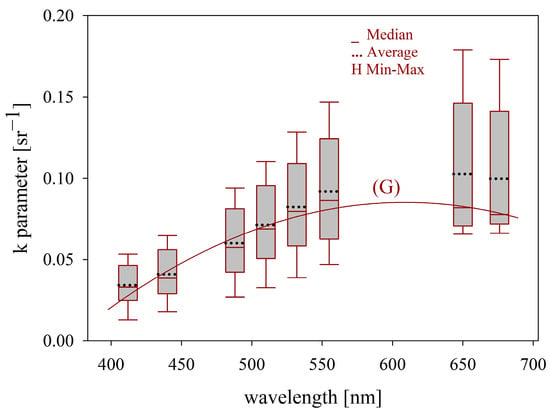
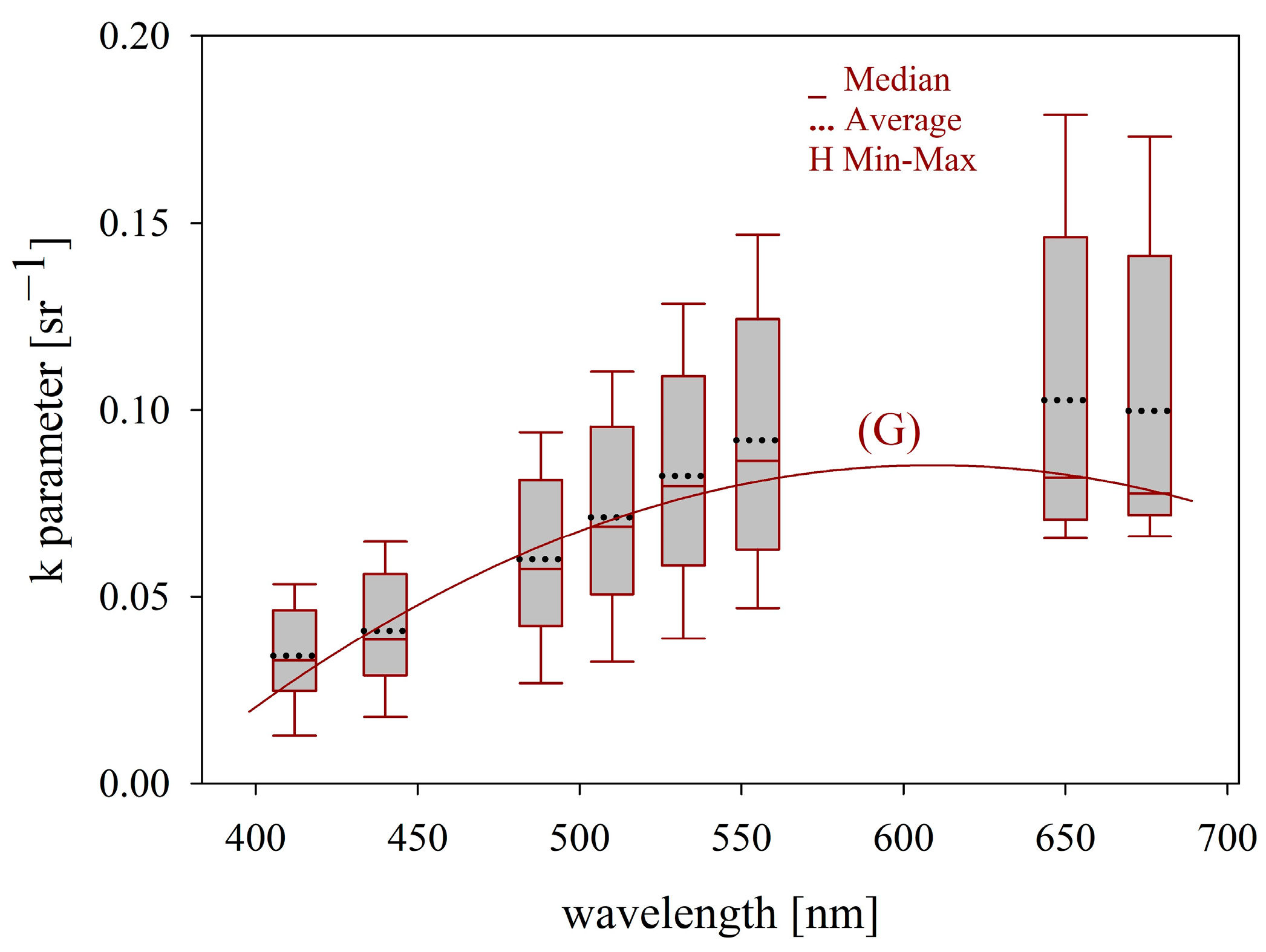
The wavelength-by-wavelength median across the six area-level medians (Table 1 (G)) increases from 0.033 sr⁻¹ at 412 nm to 0.086 sr⁻¹ at 555 nm and then decreases slightly toward the red. This pooled spectrum provides a descriptive central tendency across the six optical regimes and should not be interpreted as evidence for a universal Baltic coefficient.

3.2. Regional Differences and Spectral Trends

The comparison between areas highlights substantial differences in both the magnitude and spectral slope of k(λ) (Figure 4).

Figure 4. Spectral proxy parameter k for the six Baltic Sea areas at eight wavelengths. Curves show the area-specific quadratic fits given by Equation (8) and Table 2 (A)–(F).

Areas C and D exhibit steeper spectral increases and higher k values than the open-water area A. However, the very high constituent concentrations in Szczecin Lagoon (area F) are accompanied by comparatively low k values, demonstrating that k(λ) is not controlled by constituent concentration alone but by the balance between absorption and backscattering and by their influence on the modeled radiance field.

Despite these regional differences, all curves follow a similar concave spectral shape, with a tendency toward saturation or slight decrease at the longest wavelengths (650–676 nm). This suggests that the relationship between remote sensing reflectance and inherent optical properties becomes less sensitive to wavelength variations in the red spectral region.

3.3. Statistical Distribution of the Proxy Parameter

Figure 5 summarizes the six area-level median k values at each wavelength; the box and whisker statistics therefore describe regional spread among six medians.

Figure 5. Distribution of the six area-level median values of the effective spectral proxy coefficient k at each of eight wavelengths. The solid central mark denotes the median across the six areas, the box shows the interquartile range, and whiskers describe the spread of these six regional medians. Curve G is the quadratic fit to the wavelength-by-wavelength median values listed in Table 1 (G).

Because only six regional medians enter each wavelength specific box plot, Figure 5 is descriptive. It shows wavelength-dependent regional spread but does not provide a large-sample estimate of basin-wide variability.

The pooled median spectrum is smooth and can be represented compactly by a quadratic function. Nevertheless, the differences among the six regional medians remain substantial, and the small sample sizes for areas D–F further limit claims of regional robustness.

3.4. Quadratic Parameterization of Spectral Dependence

The spectral dependence of k(λ) for each area was approximated by the three-coefficient second-order polynomial with wavelength λ expressed in nm. Coefficients were obtained by unweighted least squares fitting directly to the eight median k values listed in the corresponding row of Table 1.

$$\mathrm{k}\left(\mathsf{\lambda }\right)=-{\mathrm{A}}_2{\mathsf{\lambda }}^2+{\mathrm{A}}_1\mathsf{\lambda }-{\mathrm{A}}_0$$

(8)

The regional quadratic fits yield R² values from 0.932 to 0.989. These coefficients of determination quantify the in-sample fit to eight smooth-area median spectral points and are not interpreted as station-level predictive skill.

The generalized row G was obtained by fitting Equation (8) directly to the eight wavelength-specific pooled medians in Table 1 (G). The resulting fit has R² = 0.954 and provides a descriptive central spectral form across the six regions.

The full-precision coefficients reproduce the Table 1 median spectra to the accuracy indicated by their R² values and ensure numerical consistency among Equation (8), Table 1 and Table 2.

Table 2. Least-squares coefficients of Equation (8), fitted directly to the eight wavelength-specific median k values in Table 1. Row G is fitted to the eight pooled median values in Table 1 (G).

Area	Region	A2 [sr−1 nm−2]	A1 [sr−1 nm−1]	A0 [sr−1]	R2
(A)	Open waters of sBS	8.311230 × 10−7	0.001085070	0.280297	0.973
(B)	Coastal waters of sBS	9.385394 × 10−7	0.001191963	0.301570	0.979
(C)	Gulf of Gdańsk	1.149858 × 10−6	0.001613170	0.430543	0.983
(D)	Puck Bay	1.150047 × 10−6	0.001752408	0.479934	0.982
(E)	Pomeranian Bay	1.985834 × 10−6	0.002376892	0.616938	0.932
(F)	Szczecin Lagoon	1.080479 × 10−7	0.000333052	0.107353	0.989
(G)	Generalized fit to Table 1 (G)	1.475249 × 10−6	0.001799144	0.463288	0.954

4. Discussion

The principal result is the wavelength- and area-dependent variation in the effective scaling coefficient k(λ) under a fixed radiative transfer configuration. The coefficient should be interpreted as a regional diagnostic of the difference between the simplified measured IOPs proxy and the Monte Carlo R_rs.

A key methodological distinction is that the two branches do not use the same representation of particle backscattering. The proxy branch uses measured Hydroscat-4 b_bp (spectrally reconstructed to the common wavelength grid), whereas the Monte Carlo branch uses measured a and b_p together with a fixed Petzold coastal water phase function; measured b_bp is not imposed in the Monte Carlo model. Consequently, k(λ) incorporates both radiative transfer effects and the difference between the measured backscattering fraction represented in the proxy and the angular scattering representation implied by the Petzold phase function. It is therefore not directly comparable to a universal f/Q-type factor.

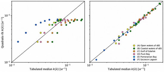
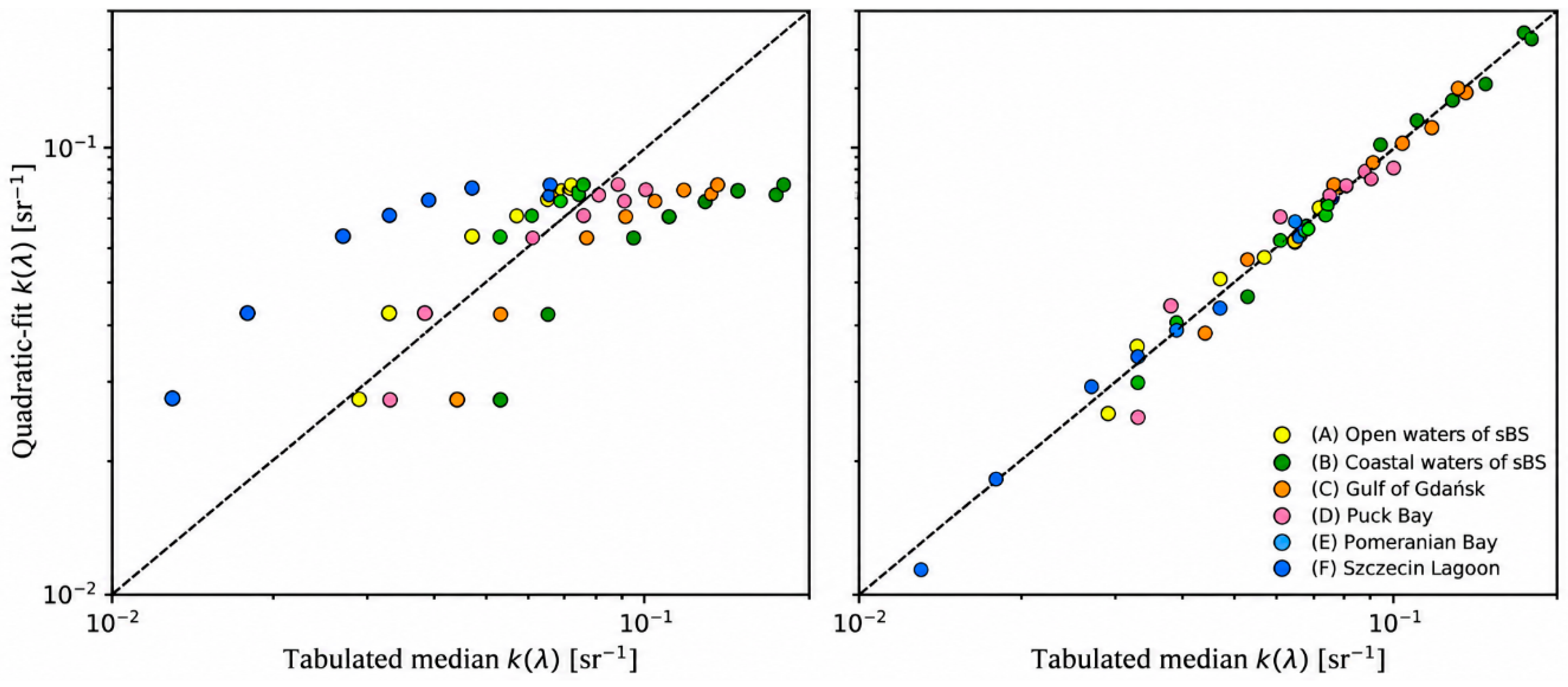
To assess internal numerical consistency without mixing the 48 regional Monte Carlo states with individual dataset-level variability, Equation (8) was re-evaluated for the six area-specific median k spectra at eight wavelengths (N = 48 area–wavelength states). The generalized fitted values were calculated from Table 2 (G), whereas the regional fitted values were calculated from Table 2 (A)–(F). Figure 6 and Figure 7 and Table 3 therefore evaluate the identical N = 48 set.

Figure 6. Numerical consistency of the quadratic spectral parameterizations for the 48 area–wavelength median states. Left: fitted k(λ) obtained from the generalized coefficients in Table 2 (G) versus the corresponding area-specific median k values in Table 1 (A)–(F). Right: fitted k(λ) obtained from the area-specific coefficients in Table 2 (A)–(F) versus the same reference medians. The dashed line denotes the 1:1 relationship.

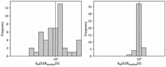
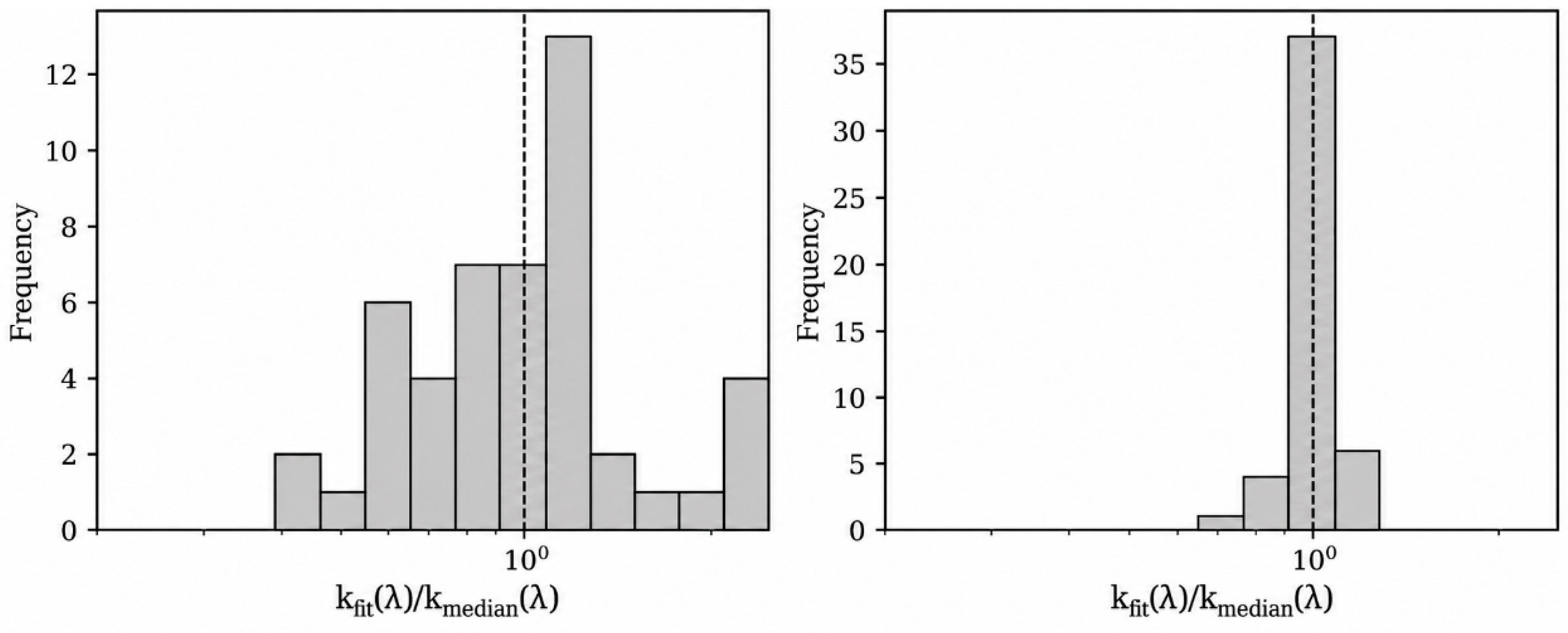
Figure 7. Frequency distributions of the ratio between quadratic-fit k(λ) and the corresponding tabulated regional median k(λ) for the same N = 48 area–wavelength states used in Figure 6. Left: generalized parameterization, Table 2 (G). Right: area-specific parameterizations, Table 2 (A)–(F). The dashed vertical line denotes unity.

Table 3. Internal numerical-consistency statistics for the 48 area–wavelength median states shown in Figure 6 and Figure 7. Relative errors are defined as 100[k_fit(λ)/k_median(λ) − 1]. The logarithmic error is ln[k_fit(λ)/k_median(λ)].

Parameterization	N	Mean Relative Error [%]	Relative RMSE [%]	Mean Logarithmic Error [−]	Standard Error Factor	Logarithmic Limits [%]
Generalized, Equation (8), Table 2 (G)	48	5.99	47.10	−0.02660	1.504	+50.40/−33.51
Area-specific, Equation (8), Table 2 (A)–(F)	48	−0.02	7.34	−0.00294	1.079	+7.92/−7.33

The generalized formulation reproduces the pooled central spectral tendency but retains substantial inter-area dispersion, whereas the area-specific equations closely reproduce the regional median spectra. Table 3 summarizes this same N = 48 consistency comparison.

For the N = 48 consistency states, the relative error is defined as ε_i = 100[k_fit,i/k_median,i − 1], and the relative RMSE is the square root of the mean squared ε_i values.

Using the corrected full-precision coefficients, the generalized formulation has a mean relative error of 5.99% and a relative RMSE of 47.10%. The area-specific equations reduce the relative RMSE to 7.34%, with a mean relative error close to zero (−0.02%). These values quantify the fidelity of the quadratic spectral representations to the tabulated regional median k spectra.

The logarithmic error is defined as ε_g,i = ln(k_fit,i/k_median,i) and is dimensionless. Its mean is the arithmetic mean of ε_g,i, while the standard error factor is obtained from the sample standard deviation of the logarithmic errors and expresses multiplicative dispersion.

The logarithmic statistics lead to the same conclusion. For the generalized formulation, the mean logarithmic error is −0.02660 and the standard error factor is 1.504, corresponding to +50.40%/−33.51% multiplicative limits. For the area-specific formulations, the corresponding values are −0.00294 and 1.079, with +7.92%/−7.33% limits.

Observational performance is assessed separately with the OCP-100 radiometric data below. The in situ radiometric measurements complement the Monte Carlo analysis by showing how the regional k(λ) parameterization performs when applied to measured R_rs.

The distributions shown in Figure 7 provide the same N = 48 diagnostic in ratio form. The generalized formulation produces a broad distribution of k_fit/k_median, whereas the area-specific formulation is tightly concentrated around unity.

4.1. Regional Variability of Water Constituents

The regional differences in k(λ) are consistent with the variability of water constituents summarized in Table 4. The investigated areas exhibit substantial differences in chlorophyll a (Chl a), total suspended solids (TSS), particulate organic matter (POM), and particulate inorganic matter (PIM), both in magnitude and variability.

Table 4. Descriptive statistics of water quality parameters (maximum, minimum, median, mean, standard deviation (SD), and coefficient of variation (CV)) for samples collected from the six Baltic Sea areas.

Area: (Number of Samples)	Parameter [Unit]	Max	Min	Median	Mean	SD	CV [%]
(A) Open waters of sBS: (36)	Chl a [mg m−3]	9.40	0.19	2.42	3.15	2.27	72
	TSS [mg L−1]	3.63	0.51	1.06	1.25	0.68	55
	POM [mg L−1]	3.50	0.47	0.99	1.08	0.63	58
	PIM [mg L−1]	1.38	0.01	0.09	0.17	0.26	153
(B) Coastal waters of sBS: (20)	Chl a [mg m−3]	6.10	0.84	2.20	2.52	1.50	60
	TSS [mg L−1]	3.50	0.73	1.19	1.38	0.70	51
	POM [mg L−1]	1.73	0.30	0.98	1.01	0.34	33
	PIM [mg L−1]	1.86	0.01	0.13	0.38	0.56	149
(C) Gulf of Gdańsk: (103)	Chl a [mg m−3]	75.86	0.76	4.83	9.84	12.38	126
	TSS [mg L−1]	20.04	0.55	2.11	3.36	3.27	97
	POM [mg L−1]	13.41	0.33	1.92	2.55	2.15	85
	PIM [mg L−1]	9.21	0.01	0.33	0.82	1.45	177
(D) Puck Bay: (10)	Chl a [mg m−3]	22.78	2.16	5.33	9.28	8.46	91
	TSS [mg L−1]	15.67	0.61	2.13	3.61	4.46	124
	POM [mg L−1]	8.29	0.43	1.88	2.33	2.30	99
	PIM [mg L−1]	7.38	0.02	0.35	1.28	2.31	181
(E) Pomeranian Bay: (12)	Chl a [mg m−3]	13.04	2.47	5.36	6.29	2.98	47
	TSS [mg L−1]	3.29	0.96	1.51	1.74	0.70	40
	POM [mg L−1]	2.74	0.74	1.16	1.31	0.55	42
	PIM [mg L−1]	0.74	0.10	0.50	0.43	0.25	58
(F) Szczecin Lagoon: (6)	Chl a [mg m−3]	76.94	3.36	16.45	32.65	32.26	99
	TSS [mg L−1]	51.64	1.93	9.06	19.36	21.27	110
	POM [mg L−1]	26.51	1.74	4.54	10.12	10.58	105
	PIM [mg L−1]	25.13	0.19	4.52	9.24	10.74	116

The open waters of the southern Baltic Sea are characterized by relatively low constituent concentrations and moderate variability, whereas the Gulf of Gdańsk and Puck Bay include observations with elevated phytoplankton and suspended matter. These patterns provide environmental context for the regional optical differences. Because areas D–F contain only 10, 12, and six datasets, respectively, their constituent statistics are interpreted descriptively.

Szczecin Lagoon provides the clearest example of this distinction. It contains the highest median and maximum concentrations of several water quality constituents, yet it exhibits the lowest absolute k values. Since k is defined as the ratio between the Monte Carlo reflectance and the dimensionless IOPs proxy b_b/(a + b_b), its magnitude depends on the relative spectral contributions of absorption and backscattering and on the resulting multiple-scattering and angular-redistribution effects, rather than on concentration magnitude alone. The Monte Carlo domain was treated as optically deep, so the observed inter-area differences cannot be attributed to bottom reflectance. Consequently, the present parameterizations should not be transferred directly to optically shallow waters in which bottom contributions are significant.

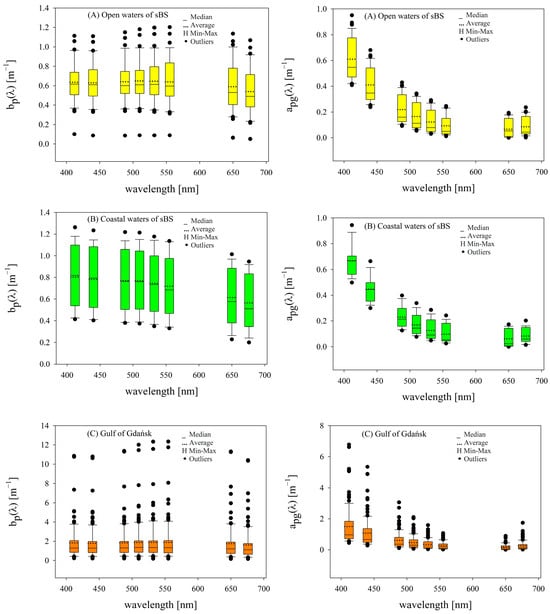
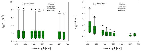
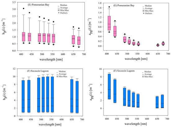
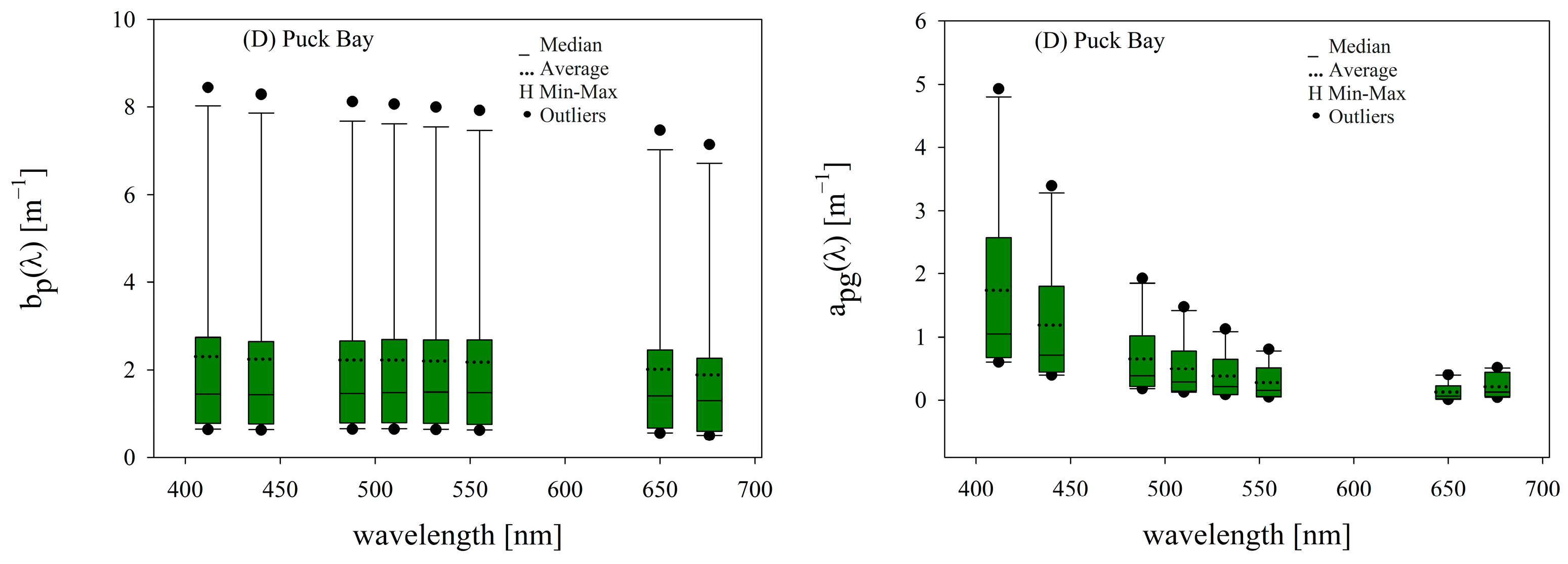
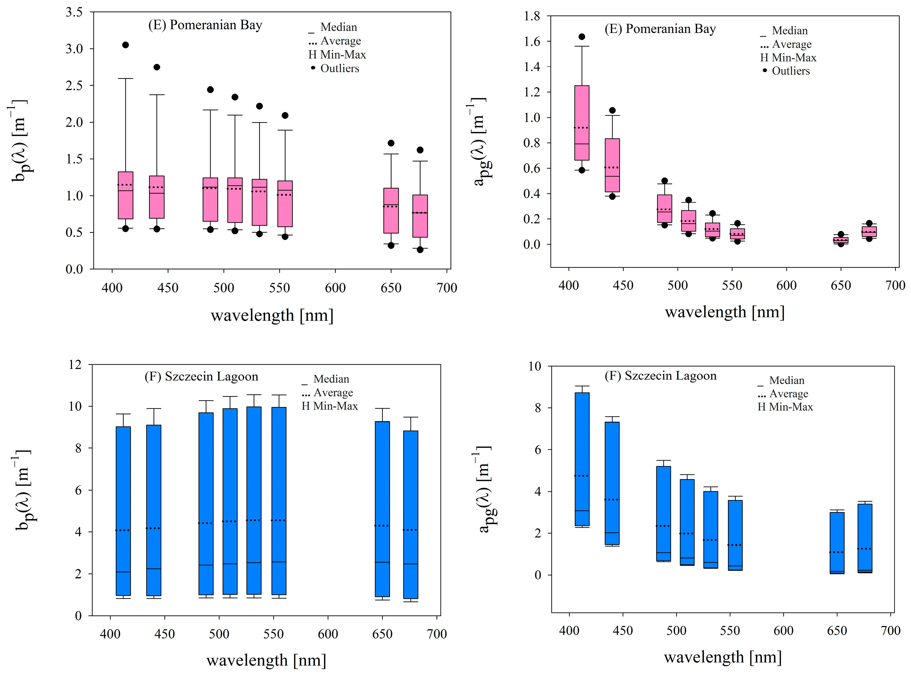
The optical variability illustrated in Figure 8 and Figure 9 further emphasizes the complexity of these environments. Figure 2 shows particulate backscattering b_bp(λ), whereas Figure 8 and Figure 9 show the distinct quantities particulate scattering b_p(λ) and combined particle plus CDOM absorption a_pg(λ). Their broad distributions and outliers demonstrate that the relative balance of scattering and absorption varies strongly within and among the investigated areas, providing the optical context for the observed variability of k(λ).

Figure 8. Particulate scattering coefficients b_p(λ) (left panels) and absorption coefficients by particles and CDOM a_pg(λ) (right panels) for areas (A–C): (A) open waters of the southern Baltic Sea, (B) coastal waters of the southern Baltic Sea, and (C) Gulf of Gdańsk, at 412, 440, 488, 510, 532, 555, 650, and 676 nm. Vertical bars represent the range of variation, H-shaped whiskers indicate the minimum and maximum values, dashes mark the median, dashed lines denote the mean, and black dots indicate outliers. The rectangles represent the interquartile range (25–75%).

Figure 9. Particulate scattering coefficients b_p(λ) (left panels) and absorption coefficients by particles and CDOM a_pg(λ) (right panels) for areas (D–F): (D) Puck Bay, (E) Pomeranian Bay, and (F) Szczecin Lagoon, at 412, 440, 488, 510, 532, 555, 650, and 676 nm. Vertical bars represent the range of variation, H-shaped whiskers indicate the minimum and maximum values, dashes mark the median, dashed lines denote the mean, and black dots indicate outliers. The rectangles represent the interquartile range (25–75%).

4.2. Validation Against Measured In Situ R_rs

Twenty-four complete OCP-100 (Satlantic) in-water radiometric spectra acquired in the Gulf of Gdańsk during March–May 2009 were available for observational evaluation. The archived OCP-100 product represents subsurface reflectance, R_rs(0⁻) = L_u(0⁻)/E_d(0⁻), i.e., the same radiometric quantity calculated by the Monte Carlo model. OCP-100 values at 420, 488, 555, and 620 nm were obtained from the adjacent measured radiometric bands using the interpolation procedure applied to this dataset [55].

For these validation records, the absorption coefficients at 420, 488, 555, and 620 nm were taken from the component resolved optical dataset previously established for the same Gulf of Gdańsk measurements [55]. At each target wavelength, total absorption was calculated as a(λ) = a_ph(λ) + a_d(λ) + a_CDOM(λ) + a_w(λ), and total backscattering as b_b(λ) = b_bp(λ) + b_bw(λ). Predicted reflectance was then calculated as R_{rs_pred}(λ) = kC(λ)(b_b(λ)/(a(λ) + b_b(λ))). The area-C coefficients were re-fitted by least squares directly to the eight median k values in Table 1 (C), yielding A₂ = 1.149858 × 10⁻⁶ sr⁻¹ nm⁻², A₁ = 0.001613170 sr⁻¹ nm⁻¹, and A₀ = 0.430543 sr⁻¹ (R² = 0.983). The corresponding kC values are 0.04415, 0.08285, 0.11058, and 0.12762 sr⁻¹ at 420, 488, 555, and 620 nm, respectively.

Agreement between predicted and observed R_rs was evaluated using Pearson’s correlation coefficient r, ordinary least-squares regression (slope and intercept), the coefficient of determination R², mean bias, root-mean-square error (RMSE), and mean absolute percentage error (MAPE). R² was obtained from the ordinary least-squares regression. Bias, RMSE, and MAPE were calculated as follows:

$$\mathrm{BIAS}={\displaystyle \frac{1}{\mathrm{N}}}{\displaystyle {\displaystyle \sum }_{\mathrm{i}=1}^{\mathrm{N}}}\left({\mathrm{R}}_{\mathrm{rs}\_\mathrm{pred},\mathrm{i}}-{\mathrm{R}}_{\mathrm{rs}\_\mathrm{obs},\mathrm{i}}\right),$$

$$\mathrm{RMSE}={\left[{\displaystyle \frac{1}{\mathrm{N}}}{\displaystyle {\displaystyle \sum }_{\mathrm{i}=1}^{\mathrm{N}}}{\left({\mathrm{R}}_{\mathrm{rs}\_\mathrm{pred},\mathrm{i}}-{\mathrm{R}}_{\mathrm{rs}\_\mathrm{obs},\mathrm{i}}\right)}^2\right]}^{{\displaystyle \frac{1}{2}}},$$

$$\mathrm{MAPE}={\displaystyle \frac{100}{\mathrm{N}}}{\displaystyle {\displaystyle \sum }_{\mathrm{i}=1}^{\mathrm{N}}}\left|{\displaystyle \frac{{\mathrm{R}}_{\mathrm{rs}\_\mathrm{pred},\mathrm{i}}-{\mathrm{R}}_{\mathrm{rs}\_\mathrm{obs},\mathrm{i}}}{{\mathrm{R}}_{\mathrm{rs}\_\mathrm{obs},\mathrm{i}}}}\right|,$$

where N denotes the number of paired predicted and observed values. The pooled calculation contains N = 96 wavelength-level pairs (24 spectra × 4 wavelengths), while the wavelength-specific calculations contain N = 24 pairs each. Reporting both levels distinguishes pooled spectral separation from station to station correspondence within individual bands.

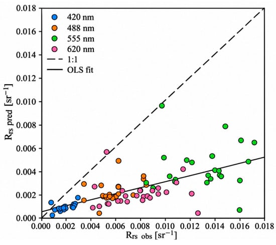
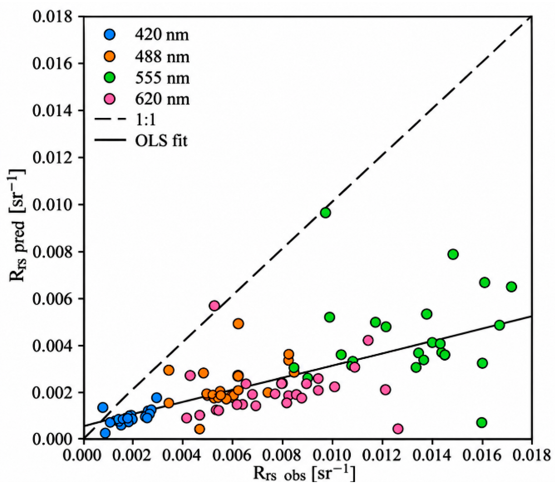
Across the 96 pooled wavelength level pairs, predicted and observed R_rs yielded r = 0.680 and R² = 0.462. The ordinary least-squares relation was R_{rs_pred} = 0.258 R_{rs_obs} + 0.000573 sr⁻¹, with mean bias = −0.00475 sr⁻¹, RMSE = 0.00590 sr⁻¹, and MAPE = 62.1% (Figure 10). The wavelength specific correlations were r = 0.628 at 420 nm, 0.443 at 488 nm, 0.140 at 555 nm, and 0.067 at 620 nm. The corresponding RMSE values were 0.00100, 0.00385, 0.00912, and 0.00635 sr⁻¹, and MAPE values were 50.7%, 60.7%, 65.6%, and 71.4%, respectively.

Figure 10. Comparison between observed in-water R_{rs_obs} and R_{rs_pred} for 24 Gulf of Gdańsk spectra at 420, 488, 555, and 620 nm. Predictions use Equation (8) with the area C coefficients re-fitted by least squares to the eight median k values in Table 1 (C): A₂ = 1.149858 × 10⁻⁶ sr⁻¹ nm⁻², A₁ = 0.001613170 sr⁻¹ nm⁻¹, and A₀ = 0.430543 sr⁻¹. The dashed line is the 1:1 relationship; the solid line is the pooled ordinary least-squares fit (N = 96 wavelength level pairs).

The pooled correlation is influenced strongly by the separation among wavelength-dependent reflectance levels and should not be interpreted as evidence of strong station-level predictive skill. Within band correspondence is weak at 555 and 620 nm, while the regression slope far below unity, negative bias, and high MAPE show substantial underestimation of absolute R_rs. The comparison therefore indicates that the regional area C formulation retains broad spectral ordering.

The OCP-100 comparison is therefore used as a observational check of the regional spectral parameterization. It shows partial retention of wavelength structure together with substantial errors in absolute magnitude and strongly wavelength-dependent station correspondence.

All Monte Carlo simulations were performed with the same Petzold coastal water phase function, Cox–Munk surface representation at a wind speed of 5 m s⁻¹, clear-sky RADTRAN illumination, a fixed solar zenith angle of 30°, and an optically deep lower boundary. Holding these conditions constant is advantageous for isolating regional optical differences, but the 30° solar zenith angle is a controlled model geometry rather than a representation of the actual March–May field geometry at 54–55°N.

The magnitude of k(λ) is sensitive to the assumed particle phase function and to the fact that measured Hydroscat b_bp is used in the proxy but not imposed in the Monte Carlo branch. Freda and Piskozub [56] showed that alternative phase functions constrained to the same backscattering ratio can modify water-leaving radiance by several percent. In the present framework, however, k should not be interpreted as a direct f/Q estimate because it also contains the difference between the measured backscattering proxy representation and the fixed Petzold angular-scattering representation. Baltic measurements may depart from the Petzold function, particularly in the backward-scattering region [54].

The use of area-specific median IOPs in the Monte Carlo simulations was adopted to define representative regional optical states and to ensure a consistent comparison among the six investigated areas. At the same time, the variability of the individual IOPs measurements was retained in the Morel proxy calculations. The Monte Carlo reference should therefore be interpreted as a regional optical representation rather than as a station-by-station reconstruction. The OCP-100 comparison complements this framework by providing an observational assessment against measured radiometric R_rs. The observed wavelength dependence of the agreement, together with the remaining differences in absolute magnitude, is consistent with the distinction between a regional parameterization and the full range of local optical and illumination conditions encountered at individual stations.

Within this framework, the quantitative interpretation of k(λ) is influenced by several factors arising at different stages of the analysis, including the assumed phase function, the use of representative regional IOPs in the Monte Carlo simulations, the spectral reconstruction of b_bp outside the Hydroscat-4 measurement bands, and station-to-station variability in the radiometric observations. These influences are not combined here into a single uncertainty term because they characterize different components of the modeling and validation procedure. Table 3 and the radiometric comparison instead provide complementary assessments of the regional parameterization. Further work can build on this framework by testing selected individual IOPs states, incorporating Baltic-specific phase functions, and examining transferability with fully independent IOPs and radiometric datasets. Once this regional optical relationship is further established, its implications for chlorophyll a, suspended matter, and CDOM retrievals can be evaluated using appropriate inversion algorithms.

5. Conclusions

This study demonstrates that the effective spectral proxy coefficient k(λ), linking the IOPs ratio b_b/(a + b_b) with remote sensing reflectance, varies systematically with both wavelength and optical environment in Baltic Sea Case-2 waters. Analysis of 187 optical datasets from six Baltic Sea areas showed that a single generalized parameterization does not fully represent the observed regional variability, whereas area-specific three-coefficient second-order polynomial formulations provide a closer representation of the corresponding regional median k spectra.

The full-precision quadratic coefficients reproduce the six regional median k spectra with a mean relative error of −0.02% and a relative RMSE of 7.34% across N = 48 area–wavelength states, compared with 5.99% and 47.10%, respectively, for the generalized fit.

The observational evaluation using 24 in situ OCP-100 spectra (N = 96 wavelength level pairs) yielded r = 0.680, R² = 0.462, a regression slope of 0.258, a mean bias of −0.00475 sr⁻¹, an RMSE of 0.00590 sr⁻¹, and a MAPE of 62.1%. The pooled comparison retained broad spectral ordering, but weak within-band correlations at 555 and 620 nm and substantial underestimation of absolute R_rs demonstrate limited station-level predictive skill.

Overall, the results support interpreting k(λ) as a wavelength- and area-dependent, configuration specific scaling coefficient rather than a universal factor. The framework provides a regional optical description that can be tested further with dataset-specific Monte Carlo simulations, Baltic-constrained phase functions, and fully independent paired IOPs–radiometry datasets.

References

- Gordon, H.R.; Brown, O.B.; Jacobs, M.M. Computed relationship between the inherent and apparent optical properties of a flat homogeneous ocean. Appl. Opt. 1975, 14, 417–427. [Google Scholar] [CrossRef] [Scilit] [PubMed]
- Morel, A.; Prieur, L. Analysis of variations in ocean color. Limnol. Oceanogr. 1977, 22, 709–722. [Google Scholar] [CrossRef] [Scilit]
- Gordon, H.R.; Morel, A. Remote Assessment of Ocean Color for Interpretation of Satellite Visible Imagery: A Review; Springer: New York, NY, USA, 1983. [Google Scholar]
- Preisendorfer, R.W. Hydrologic Optics; National Technical Information Service: Springfield, VA, USA, 1976; Volumes 1–6; pp. 1–6. [Google Scholar]
- McClain, C.R.; Franz, B.A.; Werdell, P.J. Genesis and evolution of NASA’s satellite ocean color program. Front. Remote Sens. 2022, 3, 938006. [Google Scholar] [CrossRef] [Scilit]
- Werdell, P.J.; McKinna, L.I.W.; Boss, E.; Ackleson, S.G.; Craig, S.E.; Gregg, W.W.; Lee, Z.; Maritorena, S.; Roesler, C.S.; Rousseaux, C.S. An overview of approaches and challenges for retrieving marine inherent optical properties from ocean color remote sensing. Prog. Oceanogr. 2018, 160, 186–212. [Google Scholar] [CrossRef] [Scilit] [PubMed]
- McClain, C.R.; Christian, J.R.; Signorini, S.R.; Lewis, M.R.; Asanuma, I.; Turk, D.; Dupouy-Douchement, C. Satellite ocean-color observations of the tropical Pacific Ocean. Deep Sea Res. Part II Top. Stud. Oceanogr. 2002, 49, 2533–2560. [Google Scholar] [CrossRef] [Scilit]
- Siegel, D.A.; Behrenfeld, M.J.; Maritorena, S.; McClain, C.R.; Antoine, D.; Bailey, S.W.; Bontempi, P.S.; Boss, E.S.; Dierssen, H.M.; Doney, S.C. Regional to global assessments of phytoplankton dynamics from the SeaWiFS mission. Remote Sens. Environ. 2013, 135, 77–91. [Google Scholar] [CrossRef] [Scilit]
- Kirk, J.T. Light and Photosynthesis in Aquatic Ecosystems; Cambridge University Press: Cambridge, UK, 1994. [Google Scholar]
- Gordon, H.R.; Brown, O.B.; Evans, R.H.; Brown, J.W.; Smith, R.C.; Baker, K.S.; Clark, D.K. A semianalytic radiance model of ocean color. J. Geophys. Res. Atmos. 1988, 93, 10909–10924. [Google Scholar] [CrossRef] [Scilit]
- Gordon, H.R. Inverse methods in hydrologic optics. Oceanologia 2002, 44, 9–58. [Google Scholar]
- Garver, S.A.; Siegel, D.A. Inherent optical property inversion of ocean color spectra and its biogeochemical interpretation: 1. Time series from the Sargasso Sea. J. Geophys. Res. Oceans 1997, 102, 18607–18625. [Google Scholar] [CrossRef] [Scilit]
- Morel, A.; Maritorena, S. Bio-optical properties of oceanic waters: A reappraisal. J. Geophys. Res. Oceans 2001, 106, 7163–7180. [Google Scholar] [CrossRef] [Scilit]
- Carder, K.L.; Chen, F.R.; Lee, Z.P.; Hawes, S.K.; Kamykowski, D. Semianalytic Moderate-Resolution Imaging Spectrometer algorithms for chlorophyll a and absorption with bio-optical domains based on nitrate-depletion temperatures. J. Geophys. Res. Oceans 1999, 104, 5403–5421. [Google Scholar] [CrossRef] [Scilit]
- Maritorena, S.; Siegel, D.A.; Peterson, A.R. Optimization of a semianalytical ocean color model for global-scale applications. Appl. Opt. 2002, 41, 2705–2714. [Google Scholar] [CrossRef] [Scilit] [PubMed]
- Werdell, P.J.; Franz, B.A.; Bailey, S.W.; Feldman, G.C.; Boss, E.; Brando, V.E.; Dowell, M.; Hirata, T.; Lavender, S.J.; Lee, Z. Generalized ocean color inversion model for retrieving marine inherent optical properties. Appl. Opt. 2013, 52, 2019–2037. [Google Scholar] [CrossRef] [Scilit] [PubMed]
- Lee, Z.; Carder, K.L.; Arnone, R.A. Deriving inherent optical properties from water color: A multiband quasi-analytical algorithm for optically deep waters. Appl. Opt. 2002, 41, 5755–5772. [Google Scholar] [CrossRef] [Scilit] [PubMed]
- Lo Prejato, M.; McKee, D.; Mitchell, C. Inherent optical properties-reflectance relationships revisited. J. Geophys. Res. Oceans 2020, 125, e2020JC016661. [Google Scholar] [CrossRef] [Scilit]
- Morel, A.; Gentili, B. Diffuse reflectance of oceanic waters II: Bidirectional aspects. Appl. Opt. 1993, 32, 6864–6879. [Google Scholar] [CrossRef] [Scilit] [PubMed]
- Park, Y.J.; Ruddick, K. Model of remote-sensing reflectance including bidirectional effects for case 1 and case 2 waters. Appl. Opt. 2005, 44, 1236–1249. [Google Scholar] [CrossRef] [Scilit] [PubMed]
- Hirata, T.; Højerslev, N.K. Relationship between the irradiance reflectance and inherent optical properties of seawater. J. Geophys. Res. Oceans 2008, 113, C03030. [Google Scholar] [CrossRef] [Scilit]
- Morel, A.; Antoine, D.; Gentili, B. Bidirectional reflectance of oceanic waters: Accounting for Raman emission and varying particle scattering phase function. Appl. Opt. 2002, 41, 6289–6306. [Google Scholar] [CrossRef] [Scilit] [PubMed]
- Voss, K.J.; Morel, A. Bidirectional reflectance function for oceanic waters with varying chlorophyll concentrations: Measurements versus predictions. Limnol. Oceanogr. 2005, 50, 698–705. [Google Scholar] [CrossRef] [Scilit]
- Lee, Z.P.; Carder, K.L.; Du, K.P. Effects of molecular and particle scatterings on model parameters for remote-sensing reflectance. Appl. Opt. 2004, 43, 4957–4964. [Google Scholar] [CrossRef] [Scilit] [PubMed]
- Albert, A.; Mobley, C. An analytical model for subsurface irradiance and remote sensing reflectance in deep and shallow case-2 waters. Opt. Express 2003, 11, 2873–2890. [Google Scholar] [CrossRef] [Scilit] [PubMed]
- Sathyendranath, S. (Ed.) Remote Sensing of Ocean Colour in Coastal, and Other Optically-Complex Waters; IOCCG: Dartmouth, NS, Canada, 2000. [Google Scholar]
- D’Sa, E.J.; Miller, R.L. Bio-optical properties in waters influenced by the Mississippi River during low flow conditions. Remote Sens. Environ. 2003, 84, 538–549. [Google Scholar] [CrossRef] [Scilit]
- Liu, C.C.; Miller, R.L. Spectrum matching method for estimating the chlorophyll-a concentration, CDOM ratio, and backscatter fraction from remote sensing of ocean color. Can. J. Remote Sens. 2008, 34, 343–355. [Google Scholar] [CrossRef] [Scilit]
- O’Shea, R.E.; Pahlevan, N.; Smith, B.; Boss, E.; Gurlin, D.; Alikas, K.; Kangro, K.; Kudela, R.M.; Vaičiūtė, D. A hyperspectral inversion framework for estimating absorbing inherent optical properties and biogeochemical parameters in inland and coastal waters. Remote Sens. Environ. 2023, 295, 113706. [Google Scholar] [CrossRef] [Scilit]
- Van der Woerd, H.; Pasterkamp, R. HYDROPT: A fast and flexible method to retrieve chlorophyll-a from multispectral satellite observations of optically complex coastal waters. Remote Sens. Environ. 2008, 112, 1795–1807. [Google Scholar] [CrossRef] [Scilit]
- Blondeau-Patissier, D.; Gower, J.F.R.; Dekker, A.G.; Phinn, S.R.; Brando, V.E. A review of ocean color remote sensing methods and statistical techniques for the detection, mapping and analysis of phytoplankton blooms in coastal and open oceans. Prog. Oceanogr. 2014, 123, 123–144. [Google Scholar] [CrossRef] [Scilit]
- Gregg, W.W.; Conkright, M.E.; Ginoux, P.; O’Reilly, J.E.; Casey, N.W. Ocean primary production and climate: Global decadal changes. Geophys. Res. Lett. 2003, 30, 1809. [Google Scholar] [CrossRef] [Scilit]
- Behrenfeld, M.J.; Boss, E.; Siegel, D.A.; Shea, D.M. Carbon-based ocean productivity and phytoplankton physiology from space. Glob. Biogeochem. Cycles 2005, 19, GB1006. [Google Scholar] [CrossRef] [Scilit]
- Yoder, J.; Kennelly, M. What Have We Learned About Ocean Variability from Satellite Ocean Color Imagers? Oceanography 2006, 19, 152–171. [Google Scholar] [CrossRef] [Scilit]
- McClain, C.R.; Meister, G.; Monosmith, B. Satellite Ocean Color Sensor Design Concepts and Performance Requirements. In Experimental Methods in the Physical Sciences; Donlon, C., Parr, A., Eds.; Academic Press: Cambridge, UK, 2014; Volume 47, pp. 73–119. [Google Scholar]
- Brewin, R.J.; Sathyendranath, S.; Müller, D.; Brockmann, C.; Deschamps, P.-Y.; Devred, E.; Doerffer, R.; Fomferra, N.; Franz, B.; Grant, M. The Ocean Colour Climate Change Initiative: III. A round-robin comparison on in-water bio-optical algorithms. Remote Sens. Environ. 2013, 162, 271–294. [Google Scholar]
- Konik, M.; Kowalczuk, P.; Zabłocka, M.; Makarewicz, A.; Meler, J.; Zdun, A.; Darecki, M. Empirical Relationships between Remote-Sensing Reflectance and Selected Inherent Optical Properties in Nordic Sea Surface Waters for the MODIS and OLCI Ocean Colour Sensors. Remote Sens. 2020, 12, 2774. [Google Scholar] [CrossRef] [Scilit]
- Lednicka, B.; Kubacka, M.; Freda, W.; Haule, K.; Ficek, D.; Sokólski, M. Multi-Parameter Algorithms of Remote Sensing Reflectance, Absorption and Backscattering for Coastal Waters of the Southern Baltic Sea Applied to Pomeranian Lakes. Water 2023, 15, 2843. [Google Scholar] [CrossRef] [Scilit]
- Zibordi, G.; Berthon, J.F.; Melin, F.; D’Alimonte, D.; Kaitala, S. Validation of satellite ocean color primary products at optically complex coastal sites: Northern Adriatic Sea, northern Baltic Proper, Gulf of Finland. Remote Sens. Environ. 2009, 113, 2574–2591. [Google Scholar] [CrossRef] [Scilit]
- Ostrowska, M.; Ficek, D.; Stoltmann, D.; Stoń-Egiert, J.; Zdun, A.; Kowalewski, M.; Zapadka, T.; Majchrowski, R.; Pawlik, M.; Dera, J. Ten years of remote sensing and analyses of the Baltic Sea primary production (2010–2019). Remote Sens. Appl. Soc. Environ. 2022, 26, 100715. [Google Scholar] [CrossRef] [Scilit]
- Kowalczuk, P. The absorption of yellow substance in the Baltic Sea. Oceanologia 2002, 44, 287–288. [Google Scholar]
- Reinart, A.; Kutser, T. Comparison of different satellite sensors in detecting cyanobacterial bloom events in the Baltic Sea. Remote Sens. Environ. 2006, 102, 74–85. [Google Scholar] [CrossRef] [Scilit]
- Woźniak, S.B.; Darecki, M.; Zabłocka, M.; Burska, D.; Dera, J. New simple statistical formulas for estimating surface concentrations of suspended particulate matter (SPM) and particulate organic carbon (POC) from remote-sensing reflectance in the southern Baltic Sea. Oceanologia 2016, 58, 161–175. [Google Scholar] [CrossRef] [Scilit]
- Lednicka, B.; Otremba, Z.; Sagan, S.; Piskozub, J. Modelling the Remote Sensing Reflectance for the Sea Surface Layer Using Empirical Inherent Optical Properties. Remote Sens. 2026, 18, 98. [Google Scholar] [CrossRef] [Scilit]
- Pegau, W.S.; Gray, D.; Zaneveld, J.R.V. Absorption and attenuation of visible and near-infrared light in water: Dependence on temperature and salinity. Appl. Opt. 1997, 36, 6035–6046. [Google Scholar] [CrossRef] [Scilit] [PubMed]
- Zaneveld, J.R.V.; Kitchen, J.C.; Moore, C.C. The scattering error correction of reflecting-tube absorption meters. In Proceedings of Ocean Optics XII, Bergen, Norway, 13–15 June 1994; Jaffe, J.S., Ed.; SPIE: Bellingham, WA, USA, 1994; Volume 2258, pp. 44–55. [Google Scholar]
- Maffione, R.A.; Dana, D.R. Instruments and methods for measuring the backward-scattering coefficient of ocean waters. Appl. Opt. 1997, 36, 6057–6067. [Google Scholar] [CrossRef] [Scilit] [PubMed]
- Dana, D.R.; Maffione, R.A. Determining the backward scattering coefficient with fixed-angle backscattering sensors—Revisited. In Proceedings of the Ocean Optics XVI Conference, Santa Fe, NM, USA, 18–22 November 2002. [Google Scholar]
- Morel, A. Optical properties of pure water and pure seawater. In Optical Aspects of Oceanography; Jerlov, N.G., Steemann Nielsen, E., Eds.; Academic Press: London, UK, 1974; pp. 1–24. [Google Scholar]
- Pope, R.M.; Fry, E.S. Absorption spectrum (380–700 nm) of pure water. II. Integrating cavity measurements. Appl. Opt. 1997, 36, 8710–8723. [Google Scholar] [CrossRef] [Scilit] [PubMed]
- Petzold, T.J. Volume scattering functions for selected ocean waters. In Light in the Sea; Tyler, J.E., Ed.; Dowden, Hutchinson & Ross: Stroudsburg, PA, USA, 1977. [Google Scholar]
- Cox, C.; Munk, W. Measurement of the roughness of the sea surface from photographs of the Sun’s glitter. J. Opt. Soc. Am. 1954, 44, 838–850. [Google Scholar] [CrossRef] [Scilit]
- Gregg, W.W.; Carder, K.L. A simple spectral solar irradiance model for cloudless maritime atmospheres. Limnol. Oceanogr. 1990, 35, 1657–1675. [Google Scholar] [CrossRef] [Scilit]
- Siegel, H.; Gerth, M.; Ohde, T.; Heene, T. Ocean colour remote sensing relevant water constituents and optical properties of the Baltic Sea. Int. J. Remote Sens. 2005, 26, 315–330. [Google Scholar] [CrossRef] [Scilit]
- Lednicka, B.; Kubacka, M. Semi-Empirical Model of Remote-Sensing Reflectance for Chosen Areas of the Southern Baltic. Sensors 2022, 22, 1105. [Google Scholar] [CrossRef] [Scilit] [PubMed]
- Freda, W.; Piskozub, J. Revisiting the role of oceanic phase function in remote sensing reflectance. Oceanologia 2012, 54, 29–38. [Google Scholar] [CrossRef] [Scilit]
Disclaimer/Publisher’s Note: The statements, opinions and data contained in all publications are solely those of the individual author(s) and contributor(s) and not of MDPI and/or the editor(s). MDPI and/or the editor(s) disclaim responsibility for any injury to people or property resulting from any ideas, methods, instructions or products referred to in the content. |
© 2026 by the authors. Licensee MDPI, Basel, Switzerland. This article is an open access article distributed under the terms and conditions of the Creative Commons Attribution (CC BY) license.