


Highlights
What are the main findings?
- TLS recovered more reference infrastructure objects, while UAV required less acquisition effort at the study site.
- Independent check points revealed coordinate-dependent agreement and a larger mean height difference for TLS.
What are the implications of the main findings?
- Data source choice should account for the feature class and the geometry required on an as-built map.
- A preliminary retrospective accuracy–object detection completeness score illustrates source comparison, with geometric and legal eligibility assessed separately.
Abstract
Terrestrial laser scanning (TLS) and unmanned aerial vehicle (UAV) photogrammetry provide complementary observations for infrastructure documentation, but their suitability depends on the required map features. This study compares TLS- and UAV-derived as-built products for a wastewater treatment plant with a conventional survey reference and illustrates a preliminary, retrospective, feature-level data source selection approach. Positional agreement was assessed at 30 independent check points selected purposively from details identifiable in all three products. RMSE3D was 7.51 cm for TLS and 7.66 cm for UAV; these values characterize the common observable sample rather than the accuracy of the complete infrastructure. TLS and UAV mapped 128 and 102 of 135 reference objects, corresponding to object detection completeness rates of 94.8% and 75.6%, respectively. UAV required less recorded acquisition effort, while TLS recovered more reference objects using the tested configuration. A transparent score combines planimetric accuracy and object detection completeness where both are available, with source eligibility assessed separately. The application illustrates source comparison using existing products; it does not establish improved map quality or lower production cost. A completed selected source map and a merge-all alternative were not independently evaluated.
1. Introduction
Reliable as-built mapping of engineering infrastructure increasingly relies on the integration of heterogeneous spatial datasets acquired using different surveying technologies. Recent advances in remote sensing and geodetic technologies have significantly transformed the methods used for spatial data acquisition and representation in environmental monitoring and engineering infrastructure documentation. Conventional two-dimensional geodetic products are increasingly being replaced by three-dimensional (3D) digital representations, including dense point clouds, orthophotos, and object-oriented spatial databases, which provide a more accurate and comprehensive representation of complex spatial structures. Among close-range remote sensing technologies, terrestrial laser scanning (TLS) has become one of the principal tools for modern spatial surveying owing to its capability to acquire high-density datasets with high geometric consistency [1,2]. At the same time, the rapid development and widespread availability of unmanned aerial vehicles (UAVs) have considerably expanded the capabilities of close-range remote sensing by enabling flexible, cost-effective, and high-resolution data acquisition at the local scale. UAV photogrammetry has proven particularly effective for capturing detailed surface geometry and radiometric information, complementing TLS data, especially in areas characterized by complex spatial structures [3,4]. Nevertheless, numerous studies have demonstrated that the application of a single surveying technology is often insufficient to simultaneously satisfy the requirements for positional accuracy, geometric completeness, and operational efficiency, particularly in the case of complex engineering structures [5,6,7,8].
In response to these limitations, integrated surveying approaches based on the synergistic use of terrestrial laser scanning (TLS), UAV photogrammetry, GNSS observations, and conventional geodetic measurements have become increasingly common. In this context, Integrated Surveying (IS) extends beyond simple data fusion and refers to the coordinated application of multiple surveying technologies throughout the spatial data acquisition process. Such an approach exploits the complementary strengths of individual techniques while mitigating their inherent limitations, as confirmed by recent studies in remote sensing and engineering geodesy [4,7,8,9]. From a technical perspective, integration involves combining heterogeneous datasets characterized by different spatial resolutions, acquisition geometries, and data structures. Conventional surveying and GNSS provide accurate reference observations, and TLS delivers dense three-dimensional point clouds, whereas UAV photogrammetry generates high-resolution orthophotos and image-based 3D models. Ensuring geometric consistency among these datasets requires rigorous georeferencing and registration procedures, typically based on control points established using GNSS or conventional surveying methods. As demonstrated in previous studies, inaccuracies introduced during this stage may propagate throughout the processing workflow and significantly affect the reliability of the final products [1,10].
The combined use of TLS and UAV data has proven particularly advantageous for engineering infrastructure mapping, where TLS provides highly accurate geometric representation of structural components, while UAV observations improve spatial coverage and overall completeness. Consequently, hybrid datasets are increasingly applied in as-built documentation, condition assessment, and digital representation of engineering structures [11,12,13]. However, the overlap between multiple sensing modalities inevitably introduces redundant observations and data noise, requiring dedicated filtering, optimization, and quality control procedures. Therefore, validation based on comparisons between independently acquired terrestrial and aerial datasets remains a key step in the quantitative and qualitative assessment of integrated surveying products [5,14].
High-fidelity 3D models generated from integrated datasets are gradually replacing conventional two-dimensional maps in engineering documentation and infrastructure management. They enable more intuitive interpretation of spatial relationships and support advanced analyses, including as-built mapping, structural condition assessment, and integration with Building Information Modelling (BIM) environments [9,15]. Despite the growing number of studies on integrated remote sensing techniques, relatively few have systematically evaluated their applicability and operational efficiency for engineering surveying, particularly through direct comparison with conventional geodetic methods.
Recent engineering applications include TLS/UAS assessment of industrial tanks [16] and UAV-based as-built building surveys [17]. Therefore, this study compares the positional agreement, object detection completeness, and recorded operational characteristics of TLS- and UAV-derived as-built products with a conventional survey reference. It also illustrates a preliminary, retrospective approach to feature-level data source comparison using the available class-specific evidence. The objective is to describe the complementary capabilities and limitations of the two methods using the tested configuration. This study does not independently evaluate an assembled selected source map or compare its performance with a merge-all product.
2. Materials and Methods
2.1. Study Area and Object Description
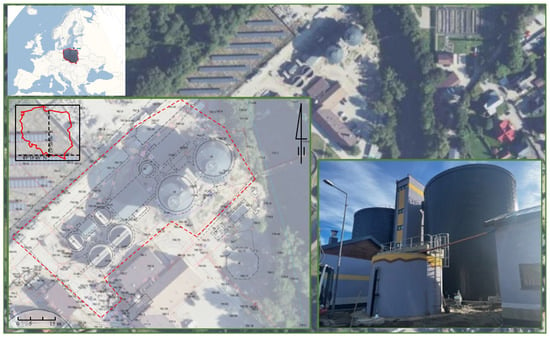
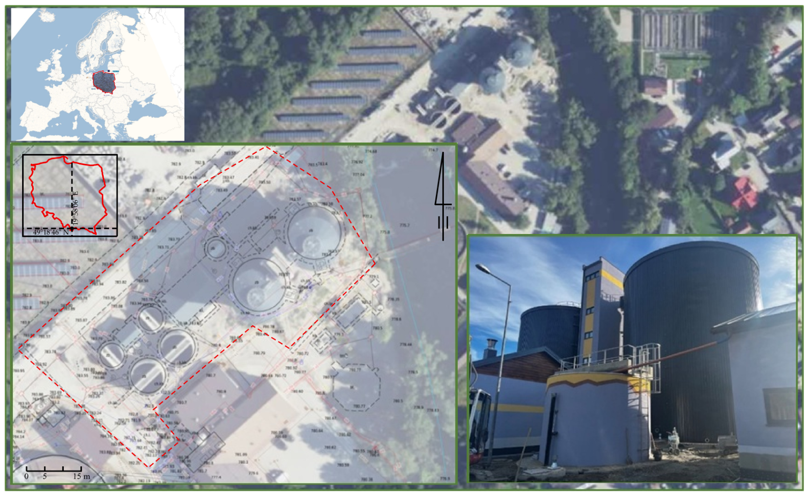
This study was conducted at an operational wastewater treatment plant representing a complex engineering infrastructure characterized by a high density of structural, technological, and linear elements. The study area comprised parts of two formally separate wastewater treatment plants, Spyrkówka and Łęgi, located in the Małopolska Voivodeship, within the administrative boundaries of the city of Zakopane, southern Poland (Figure 1). Although situated on opposite sides of the Cicha Woda River, the facilities operate as a single integrated technological system with a common sludge management process under the administration of Tatrzańska Komunalna Grupa Kapitałowa Ltd. (Zakopane, Poland).
Figure 1.
Localization of study area and object.
The investigated area included both the technological facilities of the treatment plants and the associated infrastructure, including interconnecting utility networks, internal roads, and surrounding site development. Facilities of this type are characterized by substantial geometric heterogeneity and a high density of objects with different spatial scales, making them a demanding test environment for integrated surveying methods. The treatment plant comprises regular engineering structures, such as sedimentation tanks, biological reactor chambers, and technological buildings, as well as geometrically complex and partially inaccessible objects, including above- and below-ground pipelines, steel structures, and process installations. In addition, the surveying process is complicated by numerous occlusions, variable illumination conditions, and the requirement to maintain uninterrupted plant operation throughout the measurement campaign.
As part of the planned modernization and expansion of the technological infrastructure, a multi-stage investment program was implemented, including the construction of a new biological treatment system for the Spyrkówka catchment, the extension of sludge treatment facilities, and the construction of anaerobic digestion chambers and associated infrastructure. The research presented in this study was carried out following the completion of the first stage of the investment, implemented entirely within the Łęgi wastewater treatment plant. This stage included the construction of new technological facilities, together with numerous utility relocations and new underground service connections. Completion of the construction works required a statutory as-built survey, which was performed using conventional total station surveying supported by GNSS RTK and GNSS RTN observations and adopted as the reference dataset. To evaluate the applicability of terrestrial laser scanning (TLS), UAV photogrammetry, and their integration within the Integrated Surveying Method (ISM), complementary remote sensing datasets were acquired over the same area. These datasets were georeferenced using control points established by conventional surveying methods and subsequently used to produce independent as-built maps. Finally, the resulting cartographic products were subjected to both quantitative and qualitative validation against the reference survey.
2.2. TLS Data Acquisition and As-Built Mapping
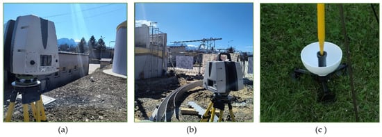
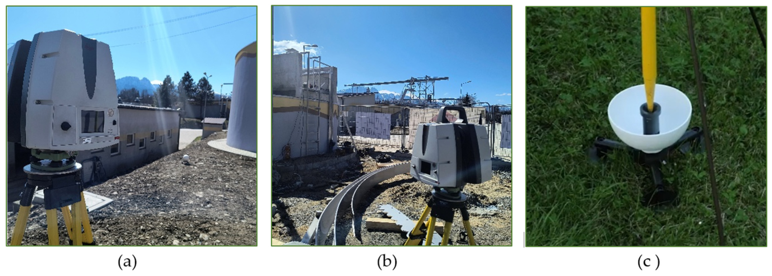
The generation of the 3D as-built map from terrestrial laser scanning (TLS) data was divided into three main stages: field survey, data processing, and cartographic mapping. The field campaign began with a preliminary site inspection and the planning of scan positions. The area of the mapped study was 2.739 ha. A total of 22 scan stations were strategically distributed to improve coverage of the study area while minimizing occlusions within the wastewater treatment infrastructure. The TLS control network consisted of 24 tie points, including 21 reference spheres and 3 planar targets (Figure 2a). The inventory comprises 135 objects in 13 classes (Table 7).
Figure 2.
TLS data capturing: (a) target network and openable reference sphere (Polish patent No. 238935 [18]); (b) Leica ScanStation P40; (c) GNSS RTK reference observations.
The reference control points, implemented as openable reference spheres, were adopted as a solution previously validated under laboratory conditions and described in the literature [19]. In the present study, the system was further evaluated under field conditions. The two-part design enables the physical realization of the sphere center, allowing its direct measurement using GNSS RTK without relying on fitting a mathematical sphere model to determine its reference position. This facilitates sphere-center identification and may improve point cloud registration and georeferencing. The effect of the target design on field accuracy was not isolated experimentally. TLS data were acquired using a Leica ScanStation P40 operating with a full 360° field of view at scan resolutions of 5 mm/10 m and 5 mm/15 m (Figure 2b), selected owing to its millimeter-level ranging accuracy and long measurement range. Both scan resolutions, 5 mm/10 m and 5 mm/15 m, were used. The reference sphere is described in [18] as the subject of Polish patent No. 238935, with Maria Makuch named as inventor. The TLS dataset was complemented by GNSS RTK observations of the control points, enabling georeferencing of the point cloud within the PL-2000/7 national coordinate reference system (Figure 2c).
Post-processing of the TLS data was performed in Cyclone REGISTER 360 PLUS (ver. 2023.0.2.r24956) and included the registration of individual scan stations into a single coherent point cloud in the local coordinate system (RMS = 0.20 cm), followed by transformation to the national reference system through georeferencing (RMS = 1.70 cm). The georeferenced point cloud in the PL-2000/7 coordinate system was subsequently unified using a redundancy removal threshold of 0.003 m. The registration and georeferencing RMS values are internal fitting residuals, distinct from the independent check point differences reported below; the effect of the 0.003 m thinning threshold was not tested at alternative values.
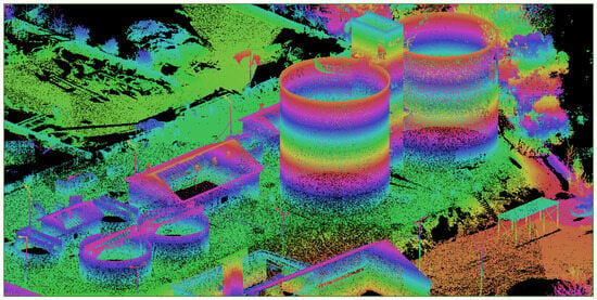
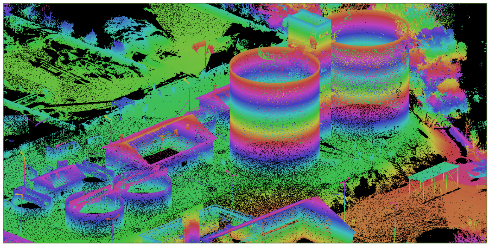
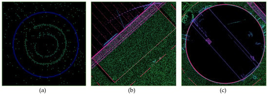
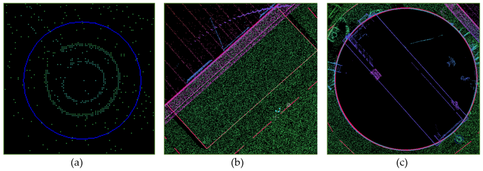
The as-built map of the wastewater treatment infrastructure was generated from the TLS dataset in the MicroStation V8i environment using the MKGEODEZY geodetic extension. A height-coded visualization of the point cloud enabled color-based classification of objects according to their elevation values, supporting accurate interpretation of their geometry and spatial position (Figure 3). The mapping process required manual extraction and delineation of individual infrastructure elements. Point features were positioned at object centroids, linear features along their geometric axes, and polygonal features according to their outer boundaries (Figure 4). The acquired TLS data enabled an accurate reconstruction of the two largest technological tanks, including the detailed geometry of steel-covered surfaces (Figure 4c), confirming the suitability of terrestrial laser scanning for producing high-detail as-built maps of complex engineering infrastructure.
Figure 3.
Height-coded visualization of the TLS point cloud used for feature identification and as-built mapping.
Figure 4.
Feature mapping from the hight-coded TLS dataset: (a) point features, (b) linear features, and (c) polygonal features.
2.3. UAV Data Acquisition and Photogrammetric Processing
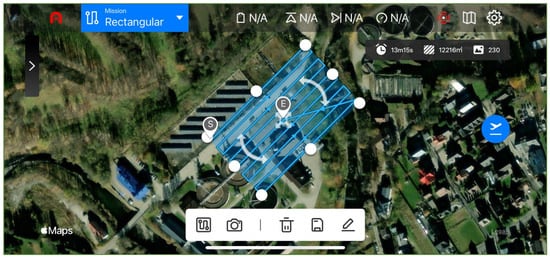
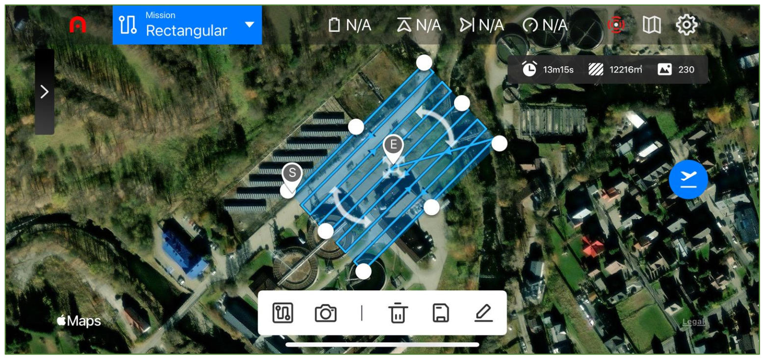
The orthophoto of the wastewater treatment plant was generated from photogrammetric data acquired using an Autel EVO II Pro unmanned aerial vehicle (UAV) equipped with a 6K digital camera and a 10.1004 mm focal length reported for the XT705 camera in Metashape. Mission planning and image acquisition were performed in automatic flight mode, enabling synchronization of the UAV survey with the terrestrial laser scanning campaign. The flight was conducted at an altitude of 40 m above ground level (AGL) with 80% forward and side overlap, ensuring sufficient image redundancy and robust aerial triangulation. The flight speed was set to 7 km h−1, while the camera optical axis was oriented vertically (90° gimbal angle) to minimize perspective distortions. These mission parameters ensured homogeneous image geometry, compatibility with the TLS dataset, and suitability for as-built mapping of engineering infrastructure. TLS and UAV data were acquired simultaneously on 3 April 2025. The flight lasted 13 min 15 s, and 229 photogrammetric images were processed (Figure 5).
Figure 5.
UAV flight mission planned in the Autel Explorer V2 application.
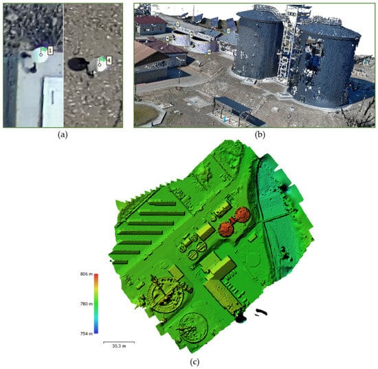
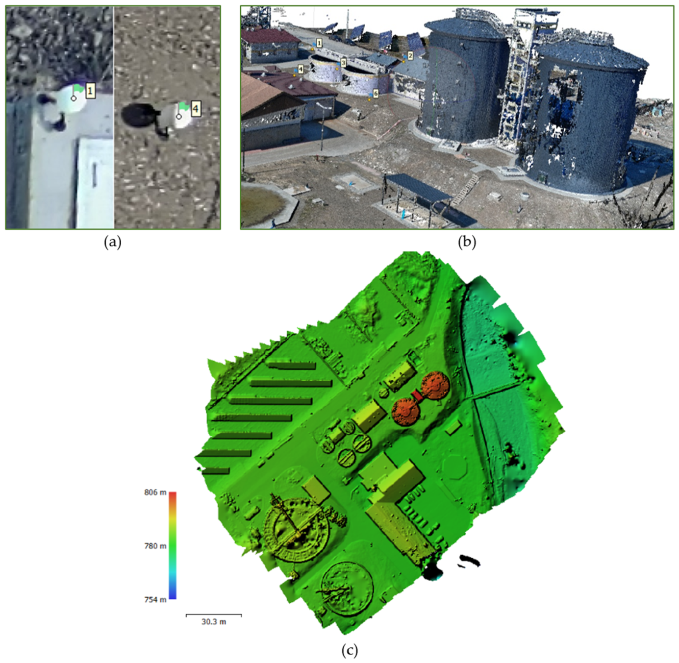
The UAV data were processed in Agisoft Metashape Professional, version 1.8.4 [20], including automatic tie-point detection, camera self-calibration, image alignment, and bundle adjustment. Georeferencing to the PL-2000/7 national coordinate reference system was achieved using five GCPs within the common survey control framework (Figure 6a). Based on the adjusted image block, a dense point cloud (Figure 6b) and a digital elevation model (DEM) (Figure 6c) were generated and subsequently used for orthorectification. Metashape Professional 1.8.4 used high alignment accuracy, generic preselection, 40,000 key points, and 4000 tie points; high-quality depth maps with mild filtering produced 80,457,290 dense points. The reported image GSD was 9.45 mm/pixel, and DEM resolution was 1.89 cm/pixel; as ground filtering is not documented, the DEM is treated as a surface model rather than a verified bare-earth DTM.
Figure 6.
UAV data processing: (a) control point network; (b) photogrammetric point cloud; (c) reconstructed surface elevation model (Metashape DEM).
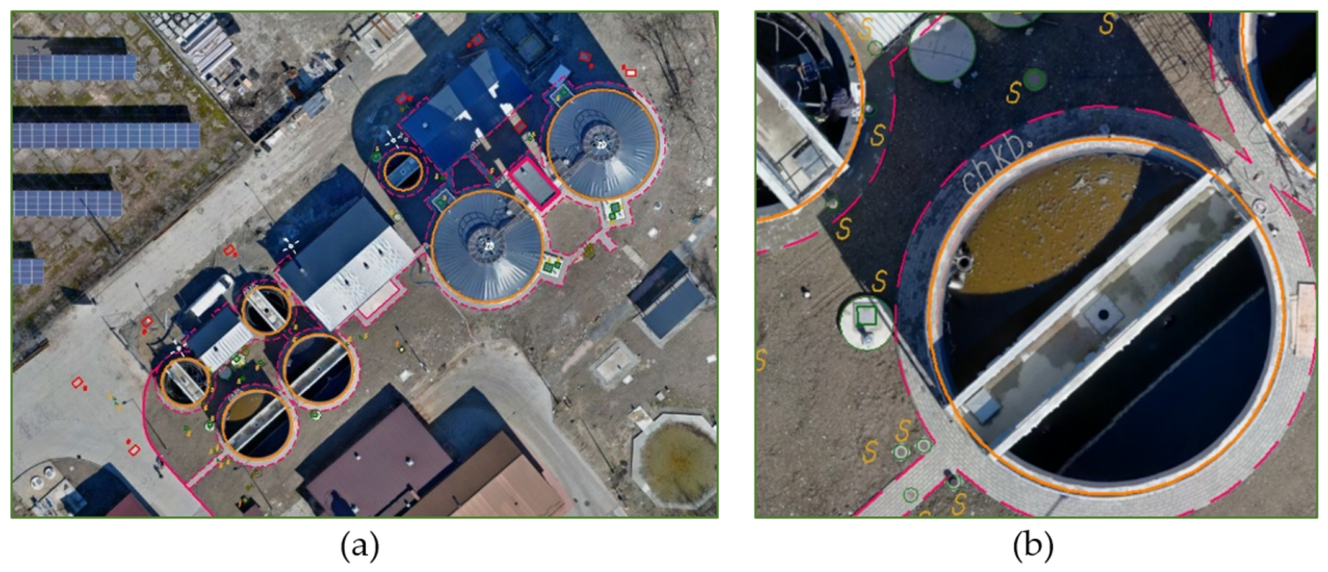
The final product was a GeoTIFF orthophoto. The reported 2.61 cm RMSE is the internal fitting error of five GCPs, with Easting, Northing, and height components of 1.69, 1.90, and 0.58 cm; it is not an independent 3D accuracy estimate of the orthophoto. The UAV-derived orthophoto proved to be an efficient source of information for mapping point, linear, and polygonal features (Figure 7), complementing the TLS dataset in open areas and supporting multi-sensor integration of spatial data. Owing to its raster representation, the orthophoto enabled more efficient visual interpretation and feature classification than direct analysis of the point cloud.
Figure 7.
Feature mapping from the UAV-derived orthophoto: (a) study area and (b) detailed view.
3. Results
The as-built maps generated from the TLS and UAV datasets were compared with the reference as-built survey completed in November 2024, following the completion of the first stage of the wastewater treatment plant expansion. The reference geodetic documentation, registered in the Polish National Geodetic and Cartographic Resource under identification number P.1217.2024.3401, served as the benchmark dataset for subsequent analyses of data complementarity and statistical agreement.
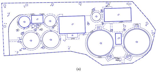
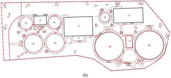
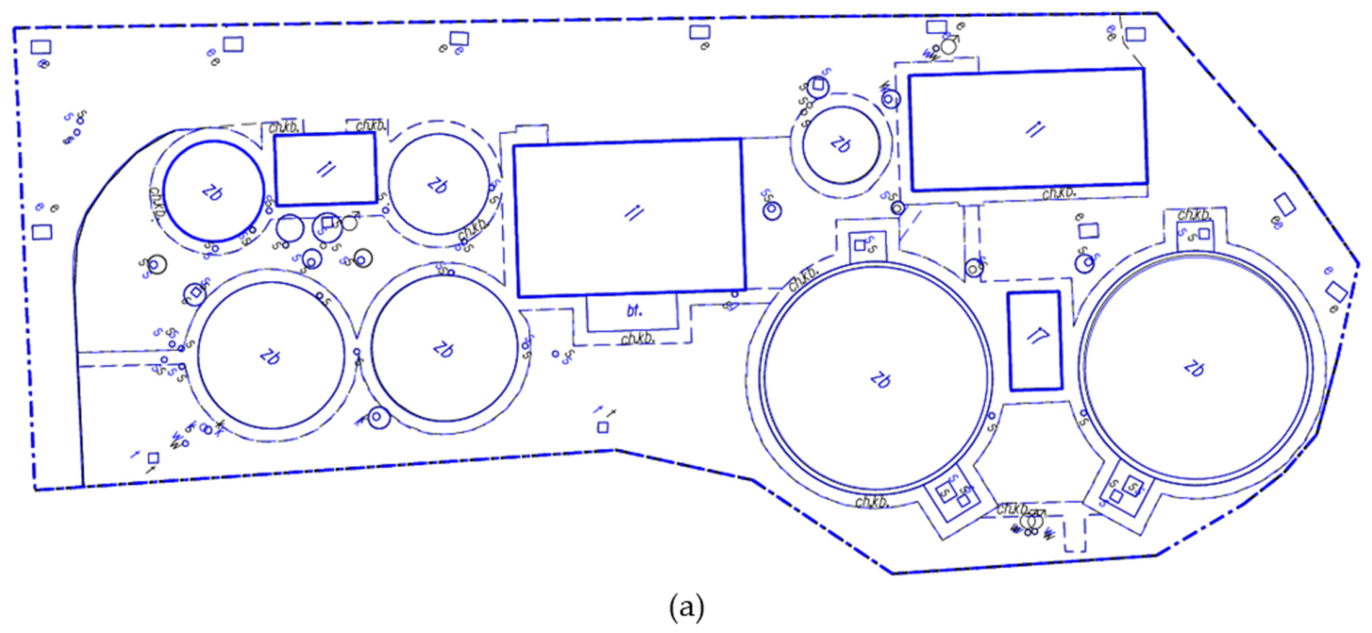
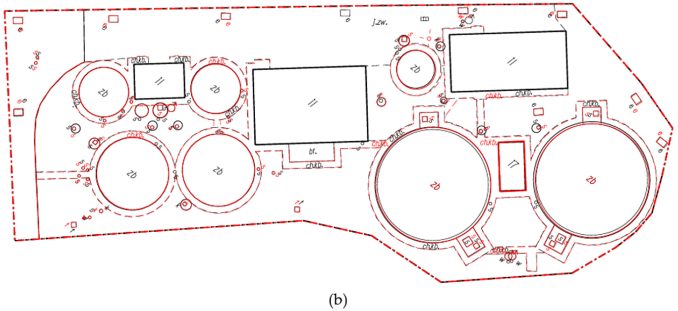
All 30 coordinates, including heights, originate from the November 2024 statutory survey, performed using a Trimble S5 total station and a Trimble R8s GNSS receiver and rigorously adjusted by least squares. The maximum reported planimetric position error and height error were each 0.01 m; these values are not treated as zero uncertainty or as specified standard deviations. Reference heights were converted from the local datum by adding 2.853 m to obtain KRON86-NHheights, then transformed to EVRF2007-NH. The check point features remained unchanged and were checked before the TLS/UAV campaign on 3 April 2025. All datasets were subsequently transformed into a common reference framework comprising the PL-2000/7 projected coordinate system and the EVRF2007-NH vertical reference system. The comparative analysis was limited exclusively to infrastructure elements constructed during the first stage of the investment (Figure 8). To assess geometric agreement and mapping completeness, the TLS-derived as-built map (Figure 8a, blue) and the UAV-derived as-built map (Figure 8b, red) were compared with the reference map obtained from conventional geodetic surveying (Figure 8, grey), enabling both qualitative and quantitative evaluation of positional accuracy and the identification of differences in the representation of individual infrastructure elements.
Figure 8.
Comparison of the conventional reference map (black) with (a) TLS results (blue) and (b) UAV results (red). Coincident colored geometry overlays the black reference geometry; elements visible only in black have no coincident colored representation at that location.
The comparison inventory contains 135 objects in 13 classes, of which 128 were mapped from TLS and 102 from UAV, corresponding to completeness of 94.8% and 75.6%. Completeness refers to the required map representation: roof visibility does not establish that a building ground footprint can be delineated. Concrete pavement edges adjoining building walls were obscured in UAV imagery, whereas paved sidewalk edges offset from buildings were observable. Zero counts indicate that the required representation could not be determined (Table 7).
3.1. Statistical Analysis
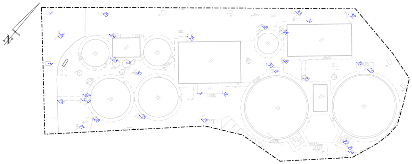
For the statistical evaluation of the generated as-built maps, a set of 30 check points representing characteristic infrastructure features was selected. Three-dimensional coordinates (X, Y, H) were extracted for each point from the three cartographic products: the reference geodetic survey, the TLS-derived as-built map, and the UAV-derived orthophoto (Figure 9). The points were selected purposively from details identifiable in all three methods and were independent of the TLS registration and UAV control or adjustment points; UAV heights were obtained from the Metashape DEM, while ICC(A,1) is the absolute agreement formulation used below. This common observable sample does not represent the accuracy of features that could not be mapped from UAV data. For the reference survey and the TLS dataset, elevation values were determined within the CAD environment, whereas UAV heights were extracted from the DEM. The statistical analysis focused on the positional accuracy, systematic error, and agreement between the investigated surveying methods. Two- and three-dimensional root mean square errors (RMSE2D and RMSE3D) were calculated to quantify positional accuracy relative to the reference survey. The Bias was subsequently determined to identify systematic deviations in the coordinate components and to distinguish systematic from random errors. Finally, the Intraclass Correlation Coefficient (ICC(A,1)) was computed to assess the agreement and reliability of the coordinates derived from the TLS and UAV datasets with respect to the reference measurements.
Figure 9.
Spatial distribution of the check points used for the statistical analysis.
Georeferencing expresses each dataset in a common coordinate reference system; registration aligns overlapping observations, while orthorectification projects images onto an elevation surface to form a planimetric raster. Agreement of products must subsequently be evaluated using points withheld from registration and adjustment. Sharing a control framework does not establish the independence of the comparison points. In this study, reference frame consistency, and comparison point independence are treated as separate requirements. The 30 points comprise 16 sanitary sewer covers, eight paved sidewalk edge points, two telecommunications chamber points, three electrical cable chamber points, and one sewer cover; accuracy conclusions are restricted to this purposive sample.
The validation of the TLS-derived as-built map and the UAV-derived as-built map was performed using a statistical sample of 30 check points. The analysis began with an evaluation of the spatial coordinate differences between the reference geodetic survey and the datasets generated using close-range remote sensing techniques. As a measure of positional accuracy, the Root Mean Square Error (RMSE) was adopted, as a measure of coordinate agreement. Based on the three coordinate datasets, two sets of coordinate differences () were calculated by comparing the reference survey with the coordinates derived from the TLS and UAV datasets, respectively [21] (Equation (1)); all reported signed differences use method minus reference, and all calculations retain n = 30:
The obtained coordinate differences were subsequently used to calculate the two-dimensional positional difference () as the square root of the sum of squared planimetric coordinate differences () (Equation (2)) and the three-dimensional positional difference () as the square root of the sum of squared coordinate differences () (Equation (3)):
At this stage, the coordinate differences were examined to identify observations exceeding the adopted comparison benchmarks. Both the TLS and UAV datasets contained only a few check points with two-dimensional positional differences greater than 0.10 m relative to the reference survey. For TLS, these were points 1 and 4 (electrical cable chambers) and point 15 (sanitary sewer manhole cover), whereas for UAV they were points 2 and 20 (sanitary sewer manhole covers). The remaining observations, representing 90.0% of the TLS sample and 93.3% of the UAV sample, were within 0.10 m. Exceeding this benchmark was not considered sufficient evidence of an erroneous observation, and all 30 points were retained in the subsequent statistical analyses. These results describe planimetric agreement for the selected check points; they do not independently establish compliance for all features represented on the as-built maps.
Before analyzing the three-dimensional positional differences, the vertical differences at the 30 check points were examined separately. For the TLS-derived map, 22 points agreed with the reference survey within an absolute height difference of 0.05 m, while the remaining eight exceeded this value. For the UAV-derived coordinates, with heights extracted from the DEM, 27 points were within 0.05 m, and three exceeded this value. The maximum absolute height difference was 0.09 m for both methods. Thus, UAV showed a higher proportion of check points within the adopted height benchmark than TLS. These comparisons do not independently certify compliance with the element-specific requirements of the Polish surveying regulations [22]. The larger TLS height differences may be associated with georeferencing or vertical reference-system transformations. However, the contribution of these factors was not isolated experimentally, and they remain possible explanations rather than established causes. The subsequent Bias analysis examines the systematic component of the observed differences.
The three-dimensional positional differences were within the descriptive 0.10 m benchmark at 25 TLS check points and 26 UAV check points. This benchmark was used to summarize the observed spatial differences rather than as a combined legal acceptance criterion. All observations, including those exceeding the benchmark, were retained in the RMSE, Bias, and ICC calculations. The assessment of the geometric accuracy of the TLS and UAV datasets was further complemented by the Root Mean Square Error (RMSE). RMSE was calculated separately for the individual coordinate components ,, as well as for the corresponding 2D and 3D positional errors, according to Equations (4)–(6) [21]:
For all 30 check points, RMSE3D was 7.51 cm for TLS and 7.66 cm for UAV (Table 1). TLS had lower RMSE2D, whereas UAV had lower RMSEh. These results describe agreement with the reference survey; the higher TLS RMSEh motivates subsequent Bias analysis without identifying its physical cause. These estimates characterize 30 purposively selected check points identifiable in all three products. They do not represent the accuracy of the complete mapped infrastructure or features that UAV photogrammetry could not represent reliably.
Table 1.
RMSE values for the geometric accuracy assessment of the TLS and UAV datasets (m).
The systematic error (Bias) for each coordinate component was calculated as the arithmetic mean of the corresponding coordinate differences (,) computed according to Equation (7):
The results of the Bias analysis and its effect on the assessment of geometric agreement are presented in Table 2:
Table 2.
Influence of systematic errors (Bias) on the geometric agreement of the TLS and UAV datasets (m).
For the planimetric coordinates derived from TLS and for the UAV X coordinate, the estimated Bias values were close to zero, indicating that the observed RMSE values were predominantly associated with the random component of the measurement errors. A different pattern was observed for the vertical component of the TLS dataset, where the estimated Bias reached −4.10 cm, closely matching the corresponding RMSEh of 4.60 cm. This result indicates that the total vertical error was largely dominated by a systematic component. To isolate the random error component (σe) from the total error expressed by the RMSE, the relationship among RMSE, Bias, and the standard deviation of the coordinate differences was applied according to the following equation (Equation (8)):
Equation (8) was subsequently used to isolate the residual RMS component after accounting for Bias (Equation (9)); this is a statistical decomposition rather than a correction of the original coordinates.
Equations (8) and (9) use denominator n for the residual mean square. After accounting for Bias, the residual RMS was 4.60, 3.68, and 2.24 cm for TLS and 3.65, 4.10, and 2.78 cm for UAV in X, Y, and H, respectively (Table 3). These values describe a statistical decomposition of the observed differences; no correction was applied to the original coordinates. For the planimetric coordinates derived from the TLS dataset (X and Y), the residual RMS values remained close to the original RMSE values, indicating a small contribution of the mean coordinate differences to the observed mean square discrepancies. A similar relationship was observed for the X coordinate of the UAV dataset. In contrast, the UAV Y-coordinate RMS decreased from 5.71 cm to 4.10 cm after accounting for Bias, indicating an appreciable systematic component. The most pronounced effect was observed for the vertical component of the TLS dataset. After accounting for Bias, the height RMS decreased from 4.64 cm to 2.24 cm, indicating that the squared mean height difference accounted for most of the observed mean square height discrepancy. For UAV, the corresponding value decreased from 3.59 cm to 2.78 cm, indicating a smaller systematic contribution. Although UAV exhibited a smaller absolute height Bias, its residual height RMS was higher than that of TLS; a smaller Bias therefore does not by itself establish greater stability of height determination (Table 3). The systematic Bias observed for the vertical component may reflect the influence of several factors, including the transformation of the reference data to a common vertical reference system and GNSS-based georeferencing performed under mountainous conditions. This interpretation is consistent with the findings of Strugarek, et al. (2026) [23], who demonstrated that the accuracy of GNSS-derived heights in mountainous regions depends primarily on the quality of the geoid/quasi-geoid model and atmospheric modelling rather than on the positioning technique itself. Their study reported local differences of 7–12 cm between quasi-geoid models, while residual tropospheric modelling errors may introduce vertical biases reaching several centimeters. However, their individual contributions were not isolated experimentally in the present study, and the Bias analysis alone cannot establish whether the discrepancy originated from georeferencing, reference height transformation, or other stages of the measurement workflow.
Table 3.
RMSres values for the geometric accuracy assessment of the TLS and UAV datasets (m).
The assessment of geometric accuracy requires consideration of the applicable surveying requirements and the characteristics of the measurement methods [24,25]. Beyond RMSE and Bias, the Intraclass Correlation Coefficient (ICC) was calculated separately for X, Y, and H to assess agreement between the TLS- and UAV-derived measurements and the reference survey. The analysis used the two-way absolute agreement, single-measurement ICC(A,1) formulation of McGraw and Wong [26]. Unlike a conventional correlation coefficient, which describes association, an absolute agreement ICC also reflects systematic differences between the compared measurements. However, ICC depends on the variability between the measured points; high values may therefore coexist with coordinate differences that are relevant to as-built surveying. Consequently, ICC was interpreted together with RMSE, Bias, and the coordinate-wise Bland–Altman analysis. ICC(A,1) was chosen because it accounts for both systematic and random sources of variability and is recommended for method comparison studies [26].
ICC estimates were calculated from the paired coordinate records, and their 95th percentile confidence intervals were obtained using 20,000 paired bootstrap resamples. All 30 check points were retained, including observations exceeding the adopted comparison benchmarks.
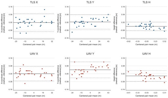
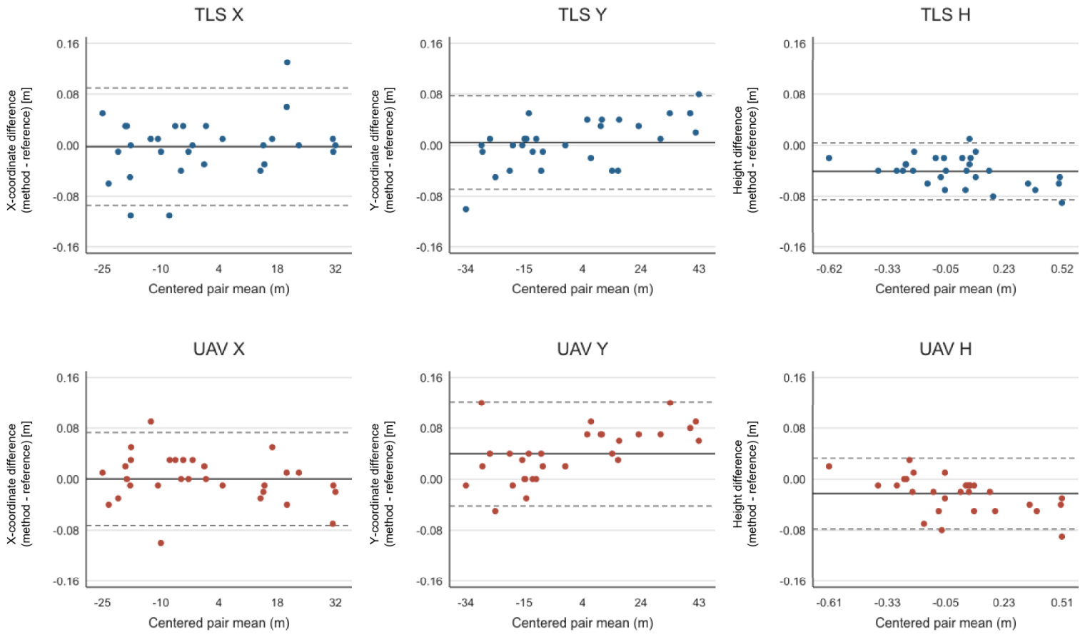
The assessment of agreement was further complemented by coordinate-wise Bland–Altman analysis, as a high ICC may reflect the spatial variability of the check points without demonstrating small coordinate differences (Figure 10, Table 4 and Table 5). For each coordinate component, method-minus-reference differences were plotted against the mean of the two measurements; the mean difference represents Bias, while the limits of agreement were calculated as the mean difference plus or minus 1.96 sample standard deviations [27]. These limits describe the approximate spread of individual differences using an approximately normal, constant variance model, whereas confidence intervals describe uncertainty in the estimated statistics. The analysis used all 30 points and 20,000 paired bootstrap resamples (seed 4531948) to obtain 95% confidence intervals for Bias, each limit of agreement, RMSE, and ICC(A,1), calculated separately for each coordinate component [27]. The intervals are conditional on the selected points and do not account for unmeasured reference uncertainty or possible spatial and within-object dependence. The reported 0.01 m maximum reference errors are not subtracted from the observed differences or propagated as standard deviations, because their probability model and covariance are not specified. The evaluation focused on descriptive summaries and estimation of agreement, including Bland–Altman mean differences and limits of agreement with bootstrap confidence intervals. No null hypothesis significance tests were reported. Proportional bias was not formally assessed; magnitude-dependent differences require further evaluation.
Figure 10.
Coordinate-wise Bland–Altman plots for TLS and UAV relative to the reference survey (n = 30). The vertical axes show X-coordinate, Y-coordinate, or height differences, calculated as method minus reference, in meters. The horizontal axes show pair means centered by a common constant within each panel, in meters. Solid lines indicate Bias, and dashed lines indicate the limits of agreement.
Table 4.
Mean differences and limits of agreement with 95% bootstrap confidence intervals (all values in m; n = 30).
Table 5.
Updated full-sample RMSE and absolute agreement ICC(A,1) estimates with 95% bootstrap confidence intervals (RMSE in m; ICC dimensionless; n = 30).
Taken together, the ICC and Bland–Altman analyses provide complementary information on agreement with the reference survey. ICC(A,1) exceeded 0.99 for X and Y, while the height values were 0.9855 for TLS and 0.9911 for UAV, with corresponding 95% bootstrap confidence intervals of 0.9732–0.9909 and 0.9820–0.9955. Despite these high coefficients, the Bland–Altman analysis revealed mean height differences of −4.07 cm for TLS and −2.27 cm for UAV, with limits of agreement of −8.52 to 0.39 cm and −7.81 to 3.28 cm, respectively. Thus, TLS exhibited a larger systematic height offset but narrower limits of agreement, whereas UAV showed a smaller mean offset with greater dispersion around that mean. These findings demonstrate why high ICC values should be interpreted alongside the magnitude and distribution of coordinate differences.
3.2. Operational Performance
The operational performance of TLS and UAV was evaluated with respect to three stages of the mapping workflow: data acquisition, data processing, and feature extraction and vectorization (Table 6). TLS data acquisition involved multi-station terrestrial laser scanning and required approximately 5–6 h of fieldwork by one operator, including the placement of targets and reference spheres. UAV acquisition required 0.5 h by one operator, including an automated flight lasting 13 min 15 s. UAV therefore required less acquisition time and fewer acquisition person-hours under the conditions of this study. Acquisition person-hours exclude control network establishment and all office-stage labor.
Table 6.
Recorded acquisition time and personnel effort; office-stage durations are reported separately.
Data processing involved several stages, including registration or image alignment, georeferencing, and generation of intermediate products. For UAV, the sum of the unique computation stages recorded in Metashape was 3 h 26 min 32 s (Table 6). This value represents computation time rather than active operator labor or a verified end-to-end processing duration. Feature extraction and vectorization required 3 h for each method. Radiometric information in the UAV orthophoto supported the identification and delineation of infrastructure features, whereas interpretation of the TLS point cloud involved inspection of cross-sections and local subsets. These differences characterize the mapping procedures, but the recorded durations do not demonstrate a time advantage for either method at the feature extraction stage.
Despite its longer acquisition time, TLS achieved higher object detection completeness, representing 128 of the 135 reference objects, compared with 102 for UAV. Roof structures and densely developed facilities limited the delineation of building footprints and other features requiring ground-level geometry from UAV data. The results therefore support the complementary use of terrestrial and aerial observations, while showing that neither dataset provided a complete representation of all required features. The available records do not support a complete economic comparison or an estimate of total workflow person-hours. Software expenditure, equipment depreciation, calibration, processing supervision, and rework were not quantified, and staffing for office stages was not documented. Accordingly, the person-hour values in Table 6 refer exclusively to data acquisition. The observed UAV advantage in acquisition effort should not be interpreted as evidence of lower total map production cost. Taken together, these findings indicate that source selection should consider the characteristics of the documented infrastructure, the required geometric representation, and the operational constraints of the survey. This provides the rationale for the feature-level data source selection framework presented in the following section, while acquisition effort remains a separate practical consideration.
3.3. Feature-Level Data Source Selection Framework
The comparison of TLS and UAV photogrammetry showed that source characteristics depend on the feature type and its required representation. A preliminary feature-level data source selection framework is proposed as a retrospective decision aid for comparing existing products. It does not constitute a validated workflow for producing a selected-source map.
The assessment uses two measurable criteria: planimetric accuracy and object detection completeness. Visibility is incorporated into completeness because it determines whether the required geometry can be identified. For example, a visible roof in UAV data does not establish that the building footprint at ground level can be determined. Acquisition time is reported separately because the available information does not allow labor input to be assigned to individual feature classes.
Planimetric accuracy was assessed against the reference survey using all independent check points within each class, including points with positional differences exceeding 0.10 m. Accuracy and completeness were expressed on a scale from 0 to 1:
where
- i—the feature class;
- j—the data source;
- Ni—the number of features of that class on the reference map;
- Nij—the number mapped from the respective source.
A reference value of t = 0.10 m was adopted to scale RMSE2D. This value does not replace verification of legal and accuracy requirements, including height accuracy. For RMSE2D ≥ t, equals zero, indicating the lowest score on the adopted scale rather than missing data. The value t = 0.10 m is a project-relevant benchmark linked to the planimetric accuracy requirement for Group I terrain details in §16 of the Polish technical standards [22]. This regulatory context motivates the scaling benchmark but does not establish robustness of the rankings or legal compliance of a completed map.
The overall data source score was defined as the weighted mean of the two criteria:
The baseline weights were wA = wC = 0.5, assigning equal importance to accuracy and completeness. They represent an explicit comparative assumption rather than expert-derived values or weights fitted to obtain a preferred method.
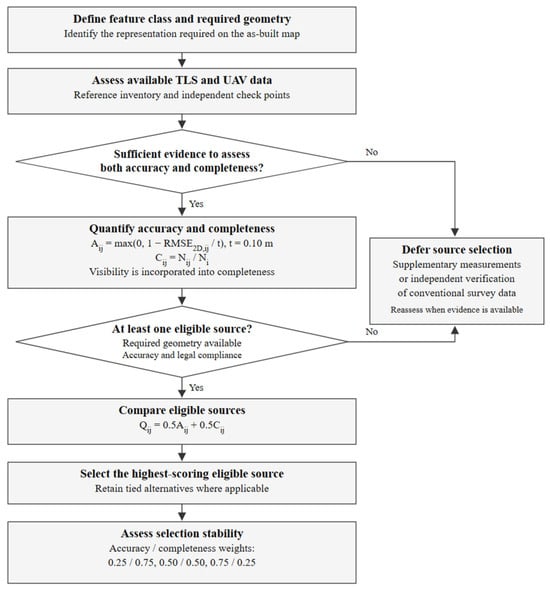
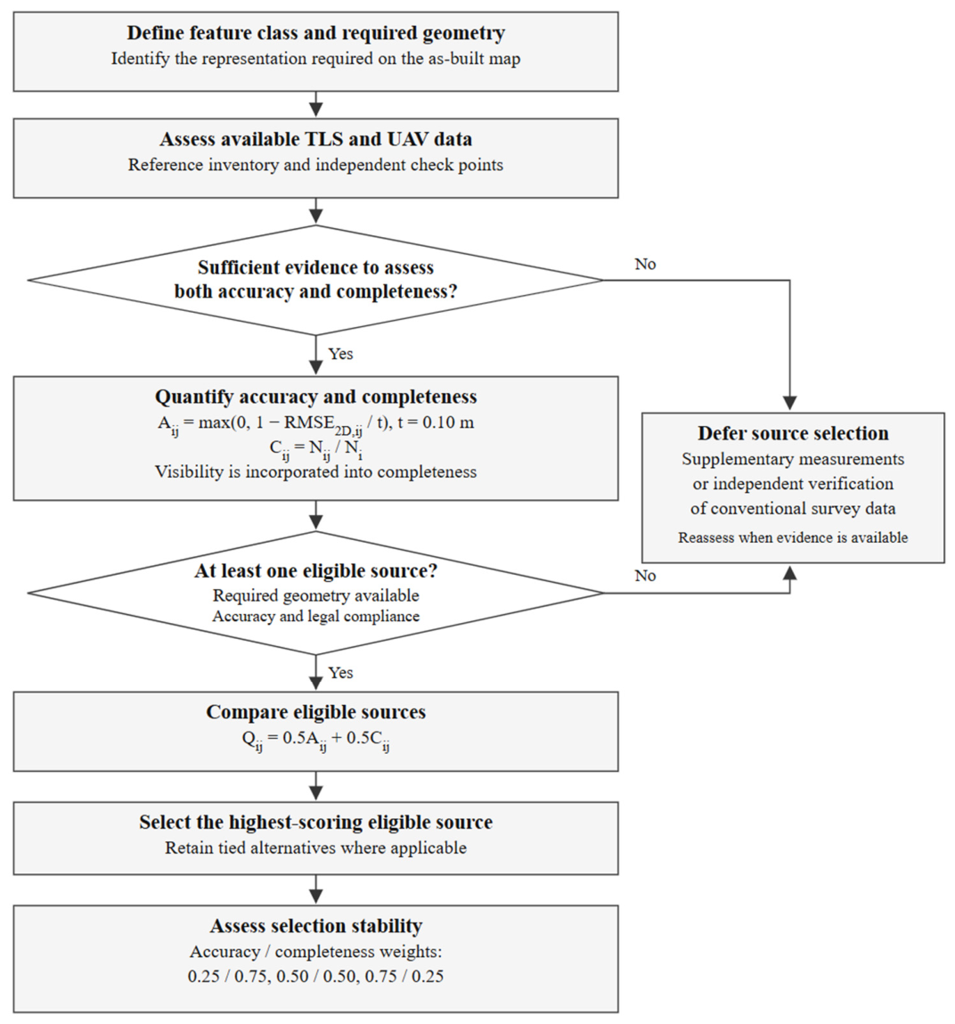
The sequence of the procedure is presented in Figure 11. After calculating the scores, source eligibility is assessed by checking whether the required geometry can be determined and whether the available evidence confirms compliance with the applicable requirements. A high score alone does not establish source eligibility.
Figure 11.
Feature-level data source selection framework based on planimetric accuracy and completeness. Visibility is incorporated into completeness. Insufficient assessment data or the absence of an eligible source requires supplementary measurements or independent verification of conventional survey data.
The framework was illustrated retrospectively using the TLS- and UAV-derived as-built maps and the conventional reference inventory. The purpose was to examine whether the measured planimetric accuracy and object detection completeness could support transparent source selection for individual feature classes. The inventory comprised 135 features in 13 classes. For each class, completeness was determined by comparing the number of features whose required map representation could be recovered from TLS or UAV with the corresponding reference count. Visibility was incorporated into this assessment through the ability to identify the required geometry.
The 30 independent check points represented five classes, for which class-specific RMSE2D values and the combined quality scores Q were calculated. Equal weights were assigned to accuracy and completeness in the baseline comparison, and alternative weights were examined to assess the stability of the resulting rankings. Only completeness was reported for the remaining eight classes, because no independent check points were available to estimate their planimetric accuracy (Table 7). Missing class-specific accuracy estimates were not replaced with zero, and no combined score was assigned to these classes.
Table 7.
Retrospective data source assessment using equal weights. Groups distinguish the extent of supporting evidence. Each pair reports TLS/UAV.
The resulting rankings illustrate retrospective comparison of existing products, subject to the required feature geometry and applicable accuracy and legal requirements. They do not demonstrate improved map accuracy, completeness, consistency, reduced redundancy, or lower production cost attributable to source selection. A completed selected source map and a merge-all alternative were not independently evaluated.
Object detection completeness is the mapped/reference object count ratio using the adopted inventory procedure. It does not quantify commission errors, recovered line length, polygon-area recovery, or geometric completeness within objects. Calculations used unrounded values. Scores based on one to three check points are illustrative and require additional validation before class-wide source selection. For n = 1, RMSE2D equals the positional difference at the single point. No score is assigned where accuracy is unassessed.
For example, 16 check points represented sanitary sewer manhole covers. RMSE2D was 5.23 cm for TLS and 6.96 cm for UAV, with completeness rates of 29/31 and 24/31, respectively. The overall scores were
The higher TLS score for this class reflected both smaller positional differences and greater completeness. UAV obtained the higher score for electrical cable chambers, where its accuracy advantage outweighed its slightly lower completeness. These results illustrate the dependence of source suitability on feature class.
The effect of the weights was examined only for (wA, wC) = (0.25, 0.75), (0.50, 0.50), and (0.75, 0.25), at a fixed t = 0.10 m. The TLS and UAV rankings remained unchanged in the five assessed classes for these scenarios. This limited assessment does not establish robustness to alternative scaling values, additional criteria, or feature-specific stakeholder priorities. These factors were not evaluated in the present study. Numerical scores for the three existing weight scenarios are provided in Supplementary Table S1.
Source selection can be expressed as
where Ji comprises sources with confirmed capability to determine the required geometry, compliance with the applicable requirements, and sufficient assessment evidence. In a tie, the equation admits more than one source. If Ji is empty or eligibility remains unresolved, selection is deferred until additional evidence is available. Conventional surveying is not assigned a perfect accuracy score by comparison with itself.
The framework links source selection to measurable results and makes the adopted assumptions explicit. Because some classes contain few check points, the results are illustrative, particularly for classes represented by one, two, or three points. The planimetric score does not establish height accuracy. Independent assessment of a map assembled from the selected sources remains necessary to validate the resulting product.
4. Discussion
The ICC(A,1) values exceeded 0.99 for the planimetric coordinate components (X and Y), indicating a high level of agreement between the TLS- and UAV-derived measurements and the reference survey. Slightly lower ICC values were observed for the vertical component (TLS: 0.9855; UAV: 0.9911), consistent with the RMSE and Bias analyses, which revealed a greater contribution of systematic error to the TLS height component. The corresponding 95% bootstrap confidence intervals were 0.9732–0.9909 for TLS and 0.9820–0.9955 for UAV. Although the vertical ICC values remained above 0.90, their interpretation should be complemented by the coordinate differences and Bland–Altman limits of agreement, as high ICC values alone do not establish whether the accuracy requirements for as-built surveying are satisfied.
The TLS height differences had a Bias of −4.07 cm and limits of agreement of −8.52 to 0.39 cm, compared with −2.27 cm and −7.81 to 3.28 cm for UAV. The updated height ICC(A,1) values were 0.9855 for TLS (95% CI: 0.9732–0.9909) and 0.9911 for UAV (95% CI: 0.9820–0.9955); thus, the high ICC values should be interpreted together with the coordinate differences and their limits of agreement, without treating them as evidence of legal acceptance.
The available records do not support a complete economic comparison or total workflow person-hour estimate. Software, equipment depreciation, calibration, processing supervision, and rework were not costed. UAV processing is reported as 3 h 26 min 32 s, the sum of the unique logged Metashape computation stages; this is computation time rather than measured operator labor or a verified end-to-end elapsed time.
The higher TLS object detection completeness and lower UAV acquisition effort reflect complementary strengths using the tested configuration. Similar complementarity has been discussed in applications combining terrestrial and aerial observations [28,29,30,31,32,33]. Here, the two-criterion framework makes that comparison explicit at feature class level, but its rankings do not demonstrate improved accuracy or reduced total cost of a completed combined map. Independent evaluation against conventional-only, TLS-only, UAV-only, and merge-all strategies would be required to assess any benefit of an assembled selected source map.
Vegetation can reduce the visibility of infrastructure in both terrestrial and aerial observations. Foliage and understory can occlude TLS sight lines and restrict sampling of the required surfaces [34,35], while vegetation cover can obscure objects in UAV imagery and affect their detectability [36]. In this framework, such effects are reflected in object detection completeness and the assessment of whether the required geometry can be recovered, rather than treated as a separately measured criterion. Their influence was not isolated at this site. Future applications could document vegetation conditions and evaluate supplementary viewpoints or measurements for obscured features.
The decision procedure could be adapted to other infrastructure, but the present scores and rankings cannot be transferred directly. Recent work on UAV bridge reconstruction and TLS–UAV heritage documentation illustrates the importance of acquisition viewpoints, complementary surface coverage, and registration [37,38,39]. Bridge applications would require attention to underside and support geometry; industrial facilities may impose access constraints around dense installations; heritage documentation may require detailed architectural surfaces. Each application would need its own feature classes, required representation, accuracy requirements, and independent assessment. The present approach provides a flexible basis for adapting feature-level data source selection to other infrastructure applications, provided that application-specific feature classes, accuracy requirements, and validation criteria are defined.
The findings are limited to one facility, one acquisition configuration, and 30 purposively selected, commonly observable check points. The conventional reference has nonzero uncertainty, and uneven class sizes limit class-wide inference. The reported bootstrap intervals are conditional on the observed sample and do not separately model spatial or within-object dependence. Independent evaluation of an assembled map, alternative acquisition geometries, and additional sites are required to assess transferability.
5. Conclusions
This study compared TLS and UAV photogrammetry with conventional survey coordinates at 30 independent, purposively selected check points observable in all three products. RMSE3D was 7.51 cm for TLS and 7.66 cm for UAV. TLS showed a larger mean height difference, but its physical cause was not established. The reported differences and uncertainty intervals characterize the selected sample rather than certifying whole-map accuracy.
TLS mapped 128 of 135 reference objects, compared with 102 for UAV. UAV required less recorded acquisition effort, whereas TLS recovered more reference objects under the tested configuration. These findings describe complementary capabilities; object counts do not establish complete geometric representation, and the acquisition records do not establish lower total production cost.
The preliminary feature-level data source selection framework illustrates retrospective comparison of available sources using planimetric accuracy and object detection completeness, with source eligibility assessed separately. The supporting evidence differs between classes, and scores based on very small samples remain illustrative. Independent evaluation of an assembled selected source map against alternative mapping strategies remains a subject for future work.
Supplementary Materials
The following supporting information can be downloaded at: https://www.mdpi.com/article/10.3390/rs18203542/s1, Table S1. Scores for the three existing weight scenarios at t = 0.10 m.
Author Contributions
Conceptualization, P.G., K.D. and M.M.; methodology, M.M., K.D. and P.G.; software, P.G., K.D. and M.G.; validation, M.M., K.D., P.G. and M.G.; formal analysis, M.M., M.G. and P.G.; investigation, M.M.; resources, M.M., K.D., P.G. and M.G.; data curation, M.M., M.G. and P.G.; writing—original draft preparation, P.G.; writing—review and editing, M.M. and P.G.; visualization, P.G. and K.D. supervision, P.G.; project administration, P.G.; funding acquisition, P.G. All authors have read and agreed to the published version of the manuscript.
Funding
This research received no external funding.
Data Availability Statement
The data used in the study are available from the corresponding author upon reasonable request.
Conflicts of Interest
Maria Makuch is the inventor named in Polish patent No. 238935 concerning the reference sphere used in this study [18].
Abbreviations
| TLS | Terrestrial laser scanning |
| UAV | Unmanned aerial vehicle |
| BIM | Building Information Modeling |
| DEM | Digital elevation model |
| 2D positional differences | |
| 3D positional differences | |
| RMSE | Root Mean Square Error |
| RMSEx | Root Mean Square Error by coordinate axes x |
| RMSEy | Root Mean Square Error by coordinate axes y |
| RMSEh | Root Mean Square Error by coordinate axes h |
| RMSE2D | 2D Root Mean Square Error |
| RMSE3D | 3D Root Mean Square Error |
| Bias | Signed error to identify systematic deviations |
| Standard deviation | |
| RMSres | Residual root mean square after accounting for Bias |
| ICC | Intraclass Correlation Coefficient |
References
- Sabzali, M.A. Comprehensive Review of Mathematical Error Characterization and Mitigation Strategies in Terrestrial Laser Scanning. Remote Sens. 2025, 17, 2528. [Google Scholar] [CrossRef] [Scilit]
- Baltsavias, E.P. Airborne Laser Scanning: Basic Relations and Formulas. Remote Sens. Environ. 1999, 68, 199–214. [Google Scholar] [CrossRef] [Scilit]
- Lefsky, M.A.; Cohen, W.B.; Parker, G.G.; Harding, D.J. LiDAR Remote Sensing for Ecosystem Studies. Remote Sens. Environ. 2002, 52, 19–30. [Google Scholar] [CrossRef] [Scilit]
- Anderson, K.; Gaston, K.J. Lightweight Unmanned Aerial Vehicles Will Revolutionize Spatial Ecology. Remote Sens. Environ. 2013, 11, 138–146. [Google Scholar] [CrossRef] [Scilit]
- Nex, F.; Remondino, F. UAV for 3D Mapping Applications: A Review. Appl. Geomat. 2014, 6, 1–15. [Google Scholar] [CrossRef] [Scilit]
- White, J.C.; Wulder, M.A.; Vastaranta, M.; Coops, N.C.; Pitt, D.; Woods, M. The Utility of Image-Based Point Clouds for Forest Inventory: A Comparison with Airborne Laser Scanning. Remote Sens. Environ. 2013, 139, 372–384. [Google Scholar] [CrossRef] [Scilit]
- Guan, S.; Zhu, Z.; Wang, G. A Review on UAV-Based Remote Sensing Technologies for Construction and Civil Applications. Drones 2022, 6, 117. [Google Scholar] [CrossRef] [Scilit]
- Gawronek, P.; Klapa, P.; Sochacki, D.; Piaseczna, K. Multi-Platform Collaboration in Integrated Surveying: Ensuring Completeness and Reliability of Geospatial Data—A Case Study. Remote Sens. 2024, 16, 4499. [Google Scholar] [CrossRef] [Scilit]
- Klapa, P.; Gawronek, P.; Gargula, T.; Sokołowska, A.; Sajdak, K. Integrating Surveying, Photogrammetric, and Remote Sensing Data to Generate Large-Scale Maps. Arch. Civ. Eng. 2025, 71, 37–50. [Google Scholar] [CrossRef] [Scilit]
- Guan, H.; Yu, Y.; Ji, Z.; Li, J.; Chang, L. Deep Learning-Based Building Point Cloud Classification for Smart Cities. Remote Sens. Environ. 2021, 261, 112484. [Google Scholar] [CrossRef] [Scilit]
- Habib, A.; Kersting, A.P.; Ruifanga, Z.; Al-Durgham, K. LiDAR Strip Adjustment Using Conjugate Planar Features. Remote Sens. Environ. 2016, 178, 124–138. [Google Scholar] [CrossRef] [Scilit]
- Sestras, P.; Bilașco, Ș.; Roșca, S.; Naș, S.; Bondrea, M. UAV-Based Photogrammetry for the Assessment of Built Infrastructure: Accuracy and Applicability. Remote Sens. 2022, 14, 623. [Google Scholar] [CrossRef] [Scilit]
- Tang, P.; Huber, D.; Akinci, B.; Lipman, R.; Lytle, A. Automatic Reconstruction of As-Built Building Information Models from Laser-Scanned Point Clouds. Autom. Constr. 2010, 19, 829–843. [Google Scholar] [CrossRef] [Scilit]
- Wang, Q.; Kim, M.K.; Cheng, J.C.P.; Sohn, H. Automated Quality Assessment of As-Is Building Information Models Using BIM and LiDAR. Autom. Constr. 2016, 68, 170–182. [Google Scholar] [CrossRef] [Scilit]
- Torresan, C.; Berton, A.; Carotenuto, F.; Di Gennaro, S.F.; Gioli, B.; Miglietta, F. Forestry Applications of UAVs in Europe: A Review. Remote Sens. Environ. 2017, 198, 612–631. [Google Scholar] [CrossRef] [Scilit]
- García-Martos, S.; García-Trenza, P.; Saura-Campos, A.; Guerrero-González, A.; Hidalgo-Castelo, F. UAS Photogrammetry and TLS Technology: A Novel Approach to Predictive Maintenance in Industrial Tank Systems. Drones 2024, 8, 215. [Google Scholar] [CrossRef] [Scilit]
- He, T.; Chen, K.; Jazizadeh, F.; Reichard, G. Unmanned aerial vehicle-based as-built surveys of buildings. Autom. Constr. 2024, 161, 105323. [Google Scholar] [CrossRef] [Scilit]
- Patent Office of the Republic of Poland. Wiadomości Urzędu Patentowego 29/2021. Granted Patent No. 238935. p. 10. Available online: https://api-ewyszukiwarka.pue.uprp.gov.pl/api/bup-or-wup/wup29_2021.pdf (accessed on 1 October 2026).
- Makuch, M.; Gawronek, P. Development and Validation of an Openable Spherical Target System for High-Precision Registration and Georeferencing of Terrestrial Laser Scanning Point Clouds. Sensors 2025, 25, 7512. [Google Scholar] [CrossRef] [Scilit] [PubMed]
- Agisoft LLC. Agisoft Metashape User Manual: Professional Edition, version 1.8; Agisoft LLC.: St. Petersburg, Russia, 2022; Available online: https://www.agisoft.com/pdf/metashape-pro_1_8_en.pdf (accessed on 13 October 2026).
- Urbančič, T.; Roškar, Ž.; Kosmatin Fras, M.; Grigillo, D. New Target for Accurate Terrestrial Laser Scanning and Unmanned Aerial Vehicle Point Cloud Registration. Sensors 2019, 19, 3179. [Google Scholar] [CrossRef] [Scilit] [PubMed]
- Minister of Development and Technology. Announcement 12 July 2022 publishing the consolidated technical standards for geodetic situational and height measurements. J. Laws 2022. Available online: https://eli.gov.pl/eli/DU/2022/1670/ogl (accessed on 13 August 2026). (In Polish)
- Strugarek, D.; Trojanowicz, M.; Mikoś, M.; Gałdyn, F.; Nowak, A.; Kur, T.; Smolak, K.; Sośnica, K. Height Determination Based on GNSS Measurements in Mountainous Areas: Contribution of the Geoid Model and Data Processing Technique to the Overall Error Budget. GPS Solut. 2026, 30, 78. [Google Scholar] [CrossRef] [Scilit]
- Habib, A.; Bang, K.I.; Aldelgawy, M.; Shin, S. Alternative Methodologies for LiDAR System Calibration. Remote Sens. 2019, 11, 467. [Google Scholar] [CrossRef] [Scilit]
- Nocerino, E.; Menna, F.; Remondino, F.; Toschi, I.; Rodríguez-Gonzálvez, P. Investigation of Indoor and Outdoor Performance of Two Portable Mobile Mapping Systems. In Videometrics, Range Imaging, and Applications XIV; International Society for Optics and Photonics (SPIE): Bellingham, WA, USA, 2017; Volume 10332. [Google Scholar] [CrossRef] [Scilit]
- McGraw, K.O.; Wong, S.P. Forming Inferences about Some Intraclass Correlation Coefficients. Psychol. Methods 1996, 1, 30–46, Correction in Psychol. Methods 1996, 1, 390. https://doi.org/10.1037/1082-989X.1.4.390. [Google Scholar] [CrossRef]
- Bland, J.M.; Altman, D.G. Statistical methods for assessing agreement between two methods of clinical measurement. Lancet 1986, 327, 307–310. [Google Scholar] [CrossRef] [Scilit]
- Tong, X.; Liu, X.; Chen, P.; Liu, S.; Luan, K.; Li, L.; Liu, S.; Liu, X.; Xie, H.; Jin, Y.; et al. Integration of UAV-Based Photogrammetry and Terrestrial Laser Scanning for Three-Dimensional Mapping and Monitoring of Open-Pit Mine Areas. Remote Sens. 2015, 7, 6635–6662. [Google Scholar] [CrossRef] [Scilit]
- Šašak, J.; Gallay, M.; Kaňuk, J.; Hofierka, J.; Minár, J. Combined Use of Terrestrial Laser Scanning and UAV Photogrammetry in Mapping Alpine Terrain. Remote Sens. 2019, 11, 2154. [Google Scholar] [CrossRef] [Scilit]
- Son, S.W.; Kim, D.W.; Sung, W.G.; Yu, J.J. Integrating UAV and TLS Approaches for Environmental Management: A Case Study of a Waste Stockpile Area. Remote Sens. 2020, 12, 1615. [Google Scholar] [CrossRef] [Scilit]
- Klapa, P.; Gawronek, P. Synergy of Geospatial Data from TLS and UAV for Heritage Building Information Modeling (HBIM). Remote Sens. 2023, 15, 128. [Google Scholar] [CrossRef] [Scilit]
- Mena, F.; Pathak, D.; Najjar, H.; Sanchez, C.; Helber, P.; Bischke, B.; Habelitz, P.; Miranda, M.; Siddamsetty, J.; Nuske, M.; et al. Adaptive Fusion of Multi-Modal Remote Sensing Data for Optimal Sub-Field Crop Yield Prediction. Remote Sens. Environ. 2025, 318, 114547. [Google Scholar] [CrossRef] [Scilit]
- Samadzadegan, F.; Toosi, A.; Dadrass Javan, F. A Critical Review on Multi-Sensor and Multi-Platform Remote Sensing Data Fusion Approaches: Current Status and Prospects. Int. J. Remote Sens. 2025, 46, 1327–1402. [Google Scholar] [CrossRef] [Scilit]
- Fareed, N.; Silva, C.A.; Numata, I.; Flores, J.P. Interdisciplinary Applications of LiDAR in Forest Studies: Advances in Sensors, Methods, and Cross-Domain Metrics. Remote Sens. 2026, 18, 219. [Google Scholar] [CrossRef] [Scilit]
- Batista, E.K.L.; Hudak, A.T.; Atkins, J.W.; Broadbent, E.N.; Brock, K.M.; Campbell, M.J.; Sánchez-López, N.; Schlickmann, M.B.; Mauro, F.; Susaeta, A.; et al. Comparing Terrestrial and Mobile Laser Scanning Approaches for Multi-Layer Fuel Load Prediction in the Western United States. Remote Sens. 2025, 17, 2757. [Google Scholar] [CrossRef] [Scilit]
- Baur, J.; Dewey, K.; Steinberg, G.; Nitsche, F.O. Modeling the Effect of Vegetation Coverage on Unmanned Aerial Vehicles-Based Object Detection: A Study in the Minefield Environment. Remote Sens. 2024, 16, 2046. [Google Scholar] [CrossRef] [Scilit]
- Jung, J.T.; Merkle, D.; Reiterer, A. Automated Camera Pose Generation for High-Resolution 3D Reconstruction of Bridges by Unmanned Aerial Vehicles. Remote Sens. 2024, 16, 1393. [Google Scholar] [CrossRef] [Scilit]
- Bac-Bronowicz, J.; Piech, I.; Wojciechowska, G. Integrated TLS-UAV Workflow for HBIM Generation in Heritage Documentation. Remote Sens. 2026, 18, 857. [Google Scholar] [CrossRef] [Scilit]
- Karkınlı, A.E.; Janowski, A.; Kaderli, L.; Gül Hüsrevoğlu, B.; Hüsrevoğlu, M. Robust Multi-Sensor Point Cloud Registration for Cultural Heritage Documentation: A Multi-Population Based Differential Evolution Approach. Remote Sens. 2026, 18, 1971. [Google Scholar] [CrossRef] [Scilit]

Disclaimer/Publisher’s Note: The statements, opinions and data contained in all publications are solely those of the individual author(s) and contributor(s) and not of MDPI and/or the editor(s). MDPI and/or the editor(s) disclaim responsibility for any injury to people or property resulting from any ideas, methods, instructions or products referred to in the content. |
© 2026 by the authors. Licensee MDPI, Basel, Switzerland. This article is an open access article distributed under the terms and conditions of the Creative Commons Attribution (CC BY) license.