Acquisition Realism in Virtual Terrestrial Laser Scanning of IFC Bridge Models: A Screening Study of Boundary-Aware Synthetic-to-Real Transfer for Point Cloud Segmentation

Highlights

What are the main findings?

• Synthetic-test benchmarks built from IFC bridge models overstate real-scan segmentation accuracy by up to +5.2 mIoU points under uniform surface sampling; reproducing terrestrial-laser-scanning acquisition effects drives this overstatement towards zero.
• After fine-tuning on real scans, only pre-training on realism-generated synthetic data improves significantly over training from scratch (+3.6 mIoU points, p = 0.025); uniform-sampling pre-training does not.

What are the implications of the main findings?

• Generator, architecture, or hyper-parameter choices validated only on synthetic test splits can reward exactly the configurations that transfer worst; the synthetic-to-real gap should be reported alongside synthetic scores.
• IFC-derived and real-scan supervision are complementary label sources—each supplies classes the other cannot—so they should be combined rather than substituted.

Abstract

Terrestrial laser scanning (TLS) of bridges supports as-built reconstruction and digital-twin maintenance, but semantic segmentation of such scans is limited by annotation cost, and synthetic point clouds generated from building information models (BIM/IFC) are the established remedy. The virtual scanner behind such data is usually a single fixed design decision validated on synthetic test splits, leaving open whether such benchmarks can be trusted and which acquisition-realism effects justify their cost. This research decomposes virtual laser scanning of four real IFC bridge models into four switchable realism factors—occlusion, incidence-angle dropout, range-dependent noise, and per-station registration error—and measures each factor’s effect, in a leave-one-factor-out screening design, on transfer to twenty real TLS bridge scans. Three findings result. (1) Synthetic-test accuracy overstates real performance by up to +5.2 mean intersection-over-union (mIoU) points: the least realistic generator scores highest on its own test split while transferring no better, and realistic acquisition drives the overstatement towards zero. (2) Boundary-aware metrics, introduced here to infrastructure point clouds, separate component-interface failures that mIoU conflates. (3) After fine-tuning on fifteen real bridges, only realism pre-training improves significantly over training from scratch (+3.6 mIoU points, Welch t(4.0) = 3.48, p = 0.025, Hedges’ g = 2.27), with a same-direction gain at component interfaces. IFC-derived and real-scan supervision are quantifiably complementary.

1. Introduction

Terrestrial laser scanning (TLS) is one of the established high-resolution acquisition techniques for the three-dimensional geometric documentation of existing bridges, alongside total stations, GNSS, mobile laser scanning, and close-range or UAV photogrammetry; the appropriate technique depends on the required accuracy, accessibility, survey scale, and purpose of the investigation [1]. Where dense TLS point clouds are acquired, semantic segmentation of the resulting point clouds is a gating step in many scan-to-BIM reconstruction, inspection-automation, and digital-twin workflows. Its practical bottleneck is labelled training data: annotating component-level classes in hundred-million-point scans is expensive, slow, and—for small or occluded components such as bearings—often impossible.

Generating synthetic training clouds from building information modelling (BIM) or city models is the established remedy, beginning with indoor scenes [2] and synthetic urban mobile scans [3]; the observation that naive surface sampling without occlusion yields unrealistic clouds was made in the industrial domain [4]. This line of work extends to bridges through procedural generators [5,6], manually modelled scenes [7,8], and virtual laser scanning with domain adaptation [9,10]. In the remote-sensing community, physically based laser-scanning simulation is mature-HELIOS++ models beam divergence, full waveforms, and platform trajectories [11], and the influence of scanning geometry on TLS point quality is quantified [12]. Within this journal, synthetic training data has been used for tree segmentation [13], realistic noise generation for virtual Doppler wind lidar has been studied as a single factor [14], and point-cloud-to-BIM reconstruction is an active topic [15]; what has not been examined is how the individual acquisition effects of a terrestrial scan jointly shape the training value of BIM-derived synthetic clouds, measured through to real-scan transfer. Labelled real-scan bridge datasets and benchmarks now exist [16,17,18], and the synthetic/real mixing ratio has been swept [19].

Two questions remain open at the intersection of these literatures. First, applied studies treat the acquisition model as one design decision (“we simulate a scanner”); its components—occlusion, incidence behaviours, range noise, registration error—have never been separated, so there is no evidence about which realism components are worth their implementation cost, nor any measurement of what each contributes to transfer. The practical stake is model selection: generators, architectures, and hyper-parameters are routinely chosen on synthetic test splits, and if those splits are not honest about real-scan difficulty, the selection itself is compromised—the winning configuration may be exactly the one that transfers worst. At most two factors (colour, mixing ratio) have been varied in one study [19]. Second, the bridge-segmentation studies surveyed here evaluate with overall accuracy (OA), mean class accuracy (mAcc), and mean intersection-over-union (mIoU) only; these area-dominated metrics are structurally insensitive to component interfaces (girder–deck, pier–pier-cap, abutment–deck), which govern downstream parametric fitting. Boundary-aware treatment is standard in general 3D vision, whether as a joint edge-prediction stream [20], a contrastive boundary loss [21], or a boundary-band evaluation metric [22]; the closest infrastructure work applies a boundary-aware loss to land transportation scenes [23] but, like the bridge literature, still reports only mIoU. Boundary quality as a reported metric has not reached infrastructure point clouds.

Relative to the nearest prior work, Yang, Fu, and Kim [9] virtually scan bridges but treat the acquisition model as fixed and report no boundary metrics; Rahman and Hoskere [10] train on synthetic reinforced-concrete (RC) bridges without separating realism factors; Kellner et al. [5] author procedural bridges, so component semantics are assigned rather than inherited from a delivery schema; Lamas et al. [6] target the truss typology with a bespoke taxonomy; the lightweight-transformer angle is already addressed by Jing et al. [24] and is therefore not pursued here. The absolute accuracies reported in this paper are not comparable to the mIoU of 89.8 reported in [9]: that work maximises accuracy on its own benchmark with a fixed acquisition model, whereas this study holds the training budget fixed and measures how acquisition-model choices shift transfer, on a public benchmark of twenty bridges with a stated, score-raising class exclusion policy applied identically to every configuration. Comparative experiments at the architecture level are nevertheless included: two established segmentation networks are run under a byte-identical training and evaluation harness (Section 3.4), so the study reports both factor-level and architecture-level comparisons on the same real benchmark.

These observations define the scope and the research questions of this study. The scope is component-level semantic segmentation of TLS point clouds of bridges, trained on synthetic clouds generated from real IFC delivery models and evaluated on real scans. Three research questions are asked. RQ1: which acquisition-realism effects of a terrestrial scan (occlusion, incidence-angle dropout, range-dependent noise, registration error) change the training and evaluation value of the synthetic data, as measured on the synthetic test split and on real-scan transfer? RQ2: can boundary-aware metrics expose component-interface failures that area-dominated metrics conflate, and under what conditions are they informative? RQ3: does acquisition realism in synthetic pre-training carry through to fine-tuning on real scans? The research gap is that no prior bridge study separates the acquisition effects (RQ1), reports boundary quality (RQ2), or connects the two through to real-scan fine-tuning (RQ3).

Table 1 summarises the closest lines of work and where this study departs from each.

Table 1. Related work by category, and how the present study differs from each.

Category (Works)	Key Characteristics	Difference of This Study
BIM-derived synthetic clouds, indoor/industrial [2,3,4]	established augmentation; realism via ray-cast simulators; single fixed acquisition setup	acquisition realism decomposed into four switchable factors and analysed in a leave-one-factor-out screening design
Synthetic bridge data [5,6,7,8]	procedurally authored or manually modelled geometry; typically 4–9-class taxonomies	real IFC delivery models; 23-class schema-traceable ontology with per-label provenance
Virtual scanning + adaptation for bridges [9,10]	maximise accuracy under one fixed acquisition model; report mIoU/mAP only	holds budget fixed, measures how acquisition choices shift transfer; reports the synthetic-to-real overstatement gap
Realism/mixing studies [14,19]	at most two factors (colour, mixing ratio) or noise realism in isolation	four TLS acquisition factors jointly, measured through to real-scan transfer and fine-tuning
Boundary-aware 3D segmentation [20,21,22,23]	edge streams, contrastive losses, boundary metrics on indoor/urban benchmarks; infrastructure work uses boundary losses but reports mIoU	boundary metrics reported for bridge point clouds, with a validation construction and a measured competence threshold
Bridge benchmarks [16,17,18]	labelled real scans and augmented databanks; domain gap quantified as an mIoU drop	benchmark used as the transfer target; gap traced to individual acquisition factors and to label-space complementarity

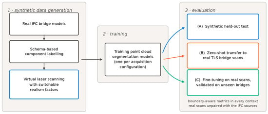
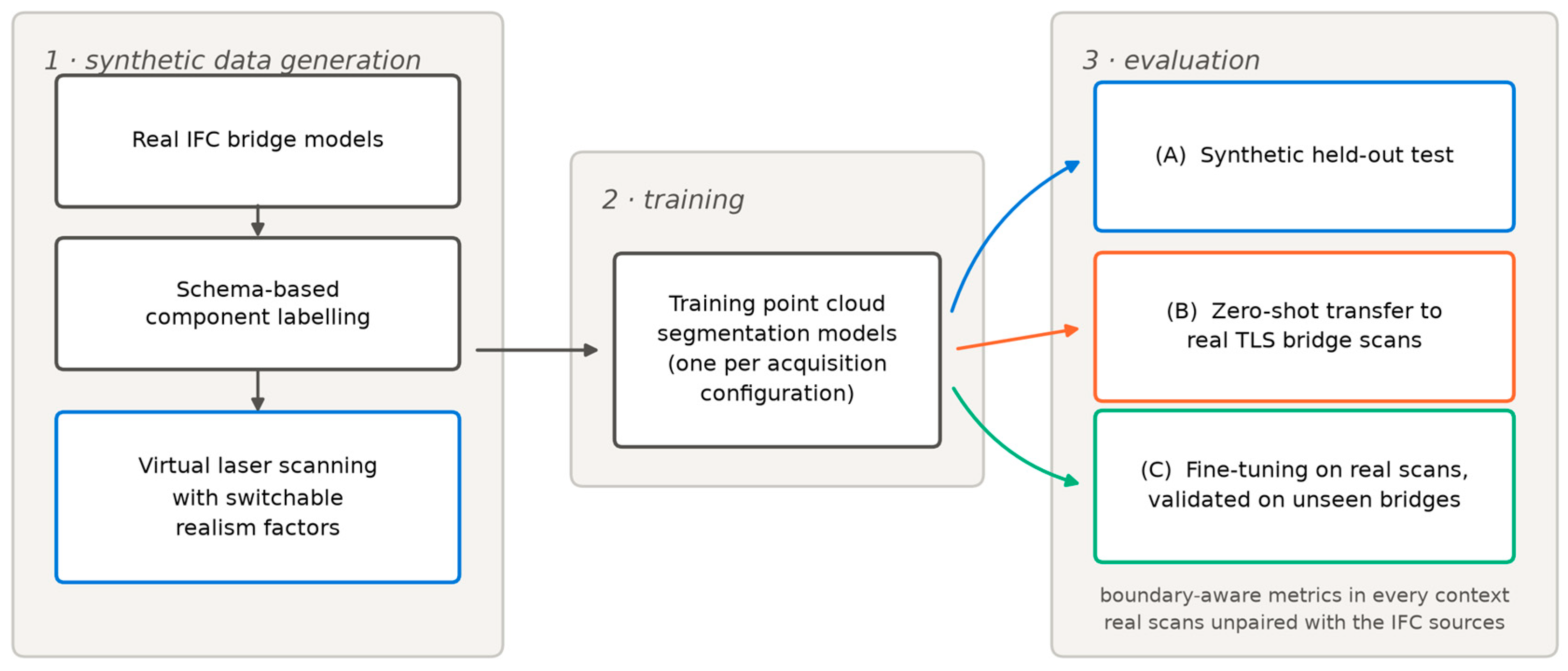
This paper contributes the following: (1) a virtual-laser-scanning acquisition model for Industry Foundation Classes (IFC) bridge data whose realism is decomposed into four independently switchable factors, analysed with a leave-one-out screening design that separates each factor’s effect; (2) evidence that synthetic-test evaluation rewards the least realistic generator while real transfer is statistically flat, making the overstatement gap the actionable quantity; (3) boundary-aware evaluation for infrastructure point clouds, with a validation construction and a measured competence threshold; (4) a schema-traceable 23-class bridge ontology resolved from IFC attributes with per-label provenance and a measured 7.8% substantive conflict rate in real delivery models; and (5) a quantified two-way complementarity between IFC-derived and real-scan supervision. All experiments use real TLS validation data (20 bridges, two scanner families) from the public SemanticBridge benchmark [18]. Figure 1 summarises the study design and, in particular, the three evaluation contexts whose scores must not be conflated: the synthetic test split, zero-shot transfer to real scans under label projection, and fine-tuning evaluated natively in the benchmark’s label space.

Figure 1. Study overview, in three stages. Generation: real IFC bridge models are component-labelled through the schema-traceable ontology and virtually scanned with independently switchable realism factors. Training: one segmentation model is trained per acquisition configuration. Evaluation: (A) a synthetic held-out test, (B) zero-shot transfer to real TLS bridge scans (predictions projected onto the benchmark’s classes), and (C) fine-tuning on real scans, validated on unseen bridges without projection. Boundary-aware metrics are computed in every context, and the real scans are unpaired with the IFC sources.

2. Materials and Methods

2.1. Source Models and Schema-Traceable Labelling

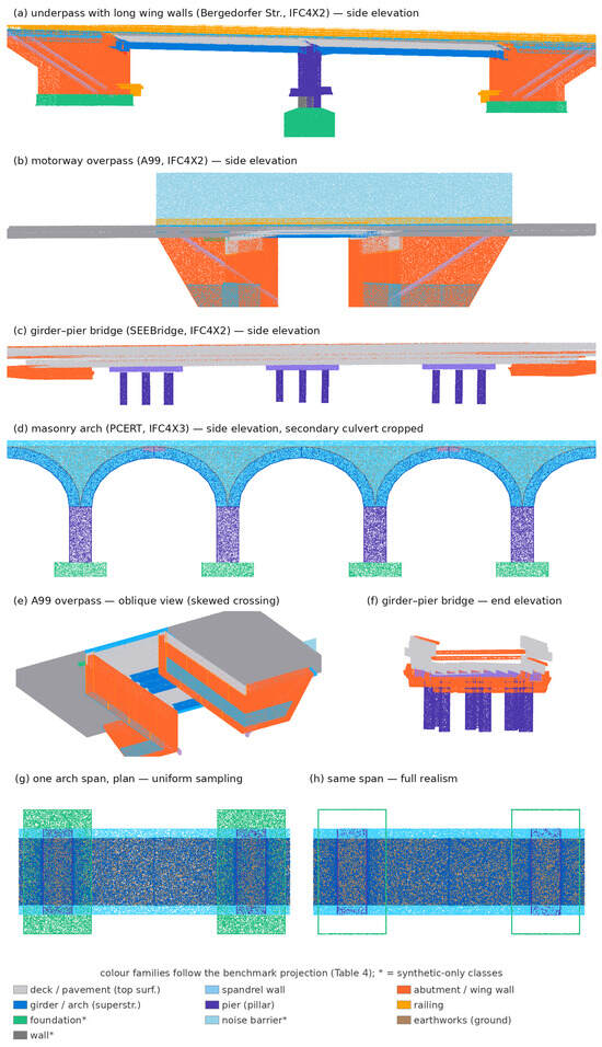
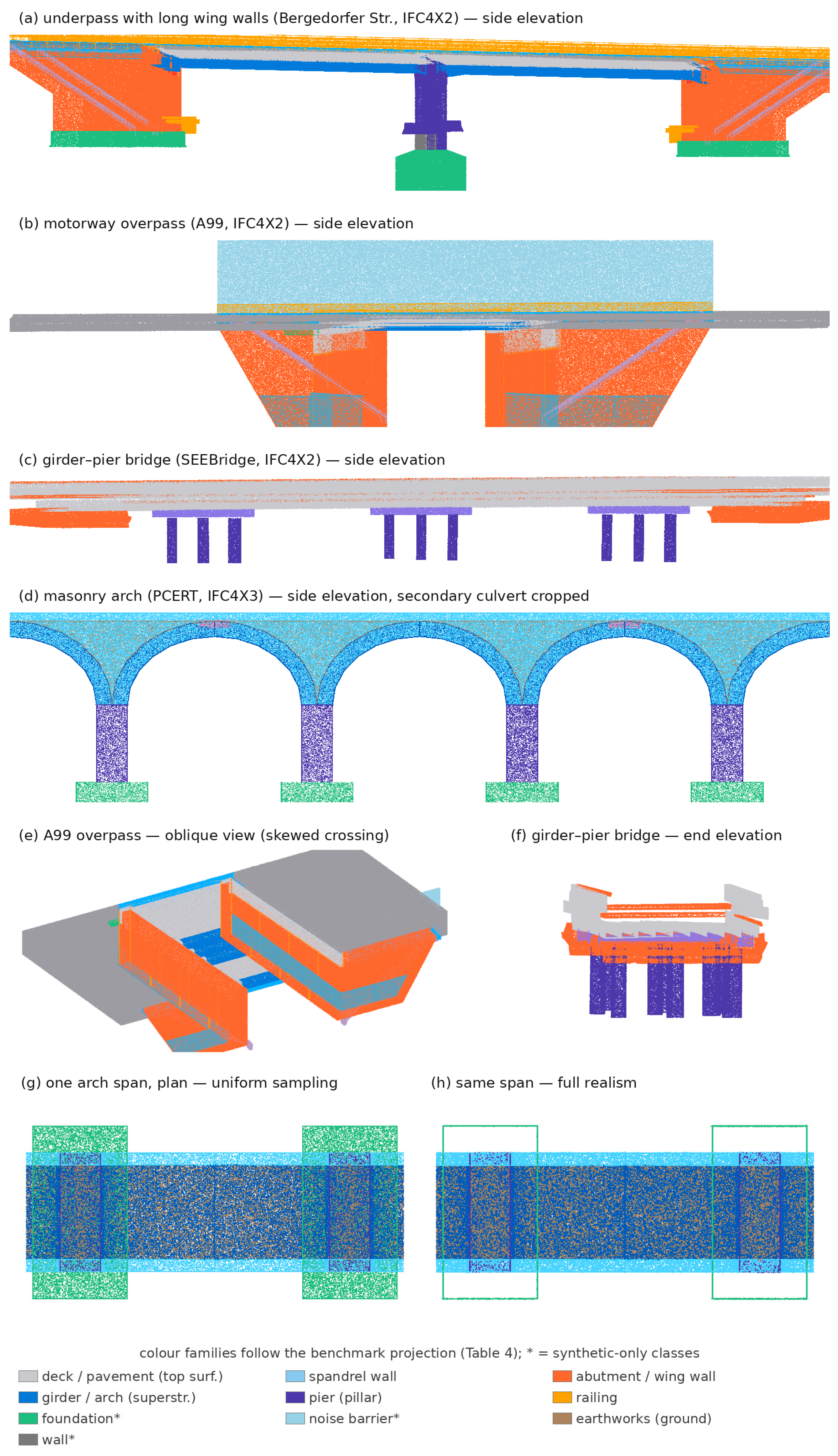
Four real bridge IFC models are used, one per structural typology (Figure 2a–d): three IFC4X2 IFC-Bridge delivery models from the German ifcinfra.de programme-Bergedorfer Straße, a road underpass with long wing walls; A99, a motorway overpass on a skewed crossing; and SEEBridge, a multi-span girder–pier bridge—and the IFC4X3_ADD2 PCERT scene of buildingSMART, a masonry-arch rail viaduct. All 456 geometric products of the four models triangulate successfully under ifcopenshell 0.8.5; after setting aside 80 semantically void products (below) and two rule-excluded auxiliary elements, 374 products enter label resolution (Table 2). Each product is resolved to one of 23 component classes by the fixed precedence PredefinedType > ObjectType > name keywords > IFC class, making every label attributable to an explicit attribute of the source model; the resolver records the producing signal per label. Over the four models, 99.2% of products resolve to a component class (signal mix: name 48.9%, PredefinedType 38.8%, ObjectType 10.4%, class 1.1%). Two properties of real delivery models are reported rather than repaired: 7.8% of products carry substantively conflicting signals (e.g., wing walls exported as IfcBeam/CORNICE while named Flügelwand, which the precedence resolves to edge beam rather than wing wall), and 80 products of one model are semantically void (no name, no type-anonymous anchor bolts), which no attribute-driven method can label; they are excluded and counted (Table 2). The conflict rate therefore upper-bounds the label noise inherited from the source models. To quantify this bound in terms of training data rather than product counts, the 29 substantively conflicting products carry 10.8% of the total sampled surface area (and, sampling being area-weighted, approximately that share of pre-occlusion points), concentrated in the abutment family (48% of abutment-class area, where the rejected alternative signals are the generic wall class or pavement) and in classes whose rejected alternative projects to the same or an unscoreable benchmark class, so that only 9.3% of surface area carries a conflict that could change its projected evaluation class. An ablation that simply deletes these products would remove almost half of the abutment-class supervision along with the suspect labels, confounding label-noise removal with class-support removal; the bound is therefore reported instead (Section 4).

Figure 2. The synthetic training data. (a–d) The four bridge typologies in axis-aligned side elevation under the full-realism acquisition model; in (d) the scene’s secondary culvert is cropped for clarity. Per-typology colour balance reflects the structures themselves (the underpass elevation is dominated by abutment/wing walls, the arch bridge by superstructure). (e) Oblique view of the A99 overpass; the crossing is skewed. (f) End elevation of the girder–pier bridge. (g,h) Plan view of one arch span under uniform sampling versus full realism: the buried foundation pads (green), fully present under uniform surface sampling, vanish under realism except for their exposed edges, and multi-station range noise roughens the remaining surfaces—the never-observed 31.2% of Section 2.2 made visible. Colour families follow the benchmark projection (Table 4); classes marked * exist only in the synthetic supervision.

Table 2. Source models and label resolution.

Model	Schema	Products	Unresolved	Subst. Conflicts	Void-Excluded
Bergedorfer Str.	IFC4X2	165	1.8%	5.5%	0
A99	IFC4X2	99	0.0%	1.0%	80
SEEBridge	IFC4X2	63	0.0%	9.5%	0
PCERT arch	IFC4X3	47	0.0%	27.7%	0

2.2. Acquisition Model with Independently Switchable Realism Factors

Dense area-weighted surface sampling with analytic normals is followed by a per-station scanner model with four independently switchable effects: (i) occlusion via a spherical z-buffer at the scanner’s angular resolution (0.036°), yielding occlusion, self-occlusion, and range-dependent density without ray–triangle intersection; (ii) incidence-angle dropout, progressive beyond 75° and total beyond 85°, following the measured incidence dependence of TLS point quality [12]; (iii) range noise, with σ growing with range and with 1/cos(incidence); and (iv) per-station registration error as a small rigid perturbation. Stations lie on ellipses around the structure at tripod height, placed from robust percentiles of the point distribution. Table 3 gives, for each effect, its exact mathematical form, its parameter values, and the probability distributions of its stochastic terms, so that the acquisition process is reproducible from the paper alone. Incidence dropout removes every return beyond θcut = 85° and removes returns between the knee θknee = 75° and the cutoff with probability p_lost(θ) = ((θ − θknee)/(θcut − θknee))². Range noise displaces each surviving return along the beam by ε~N(0, σ²) with σ(r, θ) = (σ0 + σ10·r/10 m)/max(cos θ, 0.15), σ0 = 1.2 mm, and σ10 = 1.0 mm. Registration error applies one rigid perturbation per station, with translation components drawn from N(0, (3 mm)²) and rotation angles from N(0, (0.010°)²) about the station position. Parameter magnitudes are scanner-class literature values (angular resolution from a phase-based terrestrial scanner’s quarter resolution; noise and incidence behaviour following [12]; registration at the level of target-based registration residuals); they are not calibrated to one specific instrument, and the measured effects apply to the stated magnitudes (Section 4).

Table 3. The acquisition model: exact form, parameter values, and stochastic distributions of the four switchable realism effects and of the shared acquisition geometry.

Component	Mathematical Form	Parameters
surface sampling	area-weighted, density 1/s2, analytic normals	s = 0.05 m point spacing
stations	n per ring on an ellipse from the 2%/98% coordinate percentiles, margin factor 1.35, tripod height	n = 8, 1 ring, height 1.6 m; range gate 0.6–120 m
occlusion	spherical z-buffer: nearest return per angular cell of ρ × ρ	ρ = 0.036°
incidence dropout	quadratic loss p_lost(θ) between knee and cutoff; total beyond cutoff	knee 75°, cutoff 85°
range noise	along-beam Gaussian, σ(r, θ) as in the text	σ0 = 1.2 mm, σ10 = 1.0 mm/10 m, cos θ floor 0.15
registration error	per-station rigid perturbation (R, t) about the station	t~N(0, (3 mm)2I3), angles~N(0, (0.010°)2), ZYX composition
merge	multi-station union collapsed on a voxel grid	2 cm voxel; RNG seed 42 per build

Under the full model, 31.2% of dense surface samples are never observed from any station (8.8–52.3% per bridge, driven by buried footings and deck soffits); multi-station overlap is collapsed on a 2 cm voxel grid. Under full realism, the four models yield 16.6 M labelled points (11.9 M train/4.7 M test after the split buffer of Section 2.4); per-class training support spans three orders of magnitude, from 2.7 M points (deck) to 3 k (traffic sign) and is tabulated class-by-class in Table A1 of Appendix A so that per-class transfer behaviour can be read against its supervision mass. The switchability is the experimental design: a six-cell leave-one-factor-out screening design (uniform baseline, full realism, four leave-one-out cells, three seeds each) contrasts each factor against the full-realism configuration. Figure 2 shows the resulting training data: the four bridge typologies (an underpass with long wing walls, a motorway overpass, a girder–pier bridge and a masonry arch—the last still representing a large share of the in-service European rail stock and the sole source of the arch and spandrel classes), oblique and end-elevation views, and a plan view of one arch span under uniform sampling versus full realism, in which the buried foundations disappear. Per-typology colour balance differs because the typologies differ: the underpass elevation is dominated by abutment and wing walls, the arch bridge by superstructure. Colour families follow the benchmark projection of Table 4, so the supervision visible here can be compared directly with the real-scan predictions presented in Section 3.4.

Table 4. Projection of the 23-class ontology onto the benchmark’s nine classes, applied to predictions at evaluation time.

Benchmark Class	Ontology Classes Projected onto It
top surface	deck, pavement
superstructure	girder, edge beam, arch, spandrel wall
pillar	pier, pier cap
abutment	abutment, wing wall
railing/ground/traffic sign	railing/earthworks/traffic sign
unscoreable (reported separately)	bearing, expansion joint, foundation, drainage, noise barrier, steel detail, stairs, wall

2.3. Segmentation Networks and Training

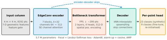
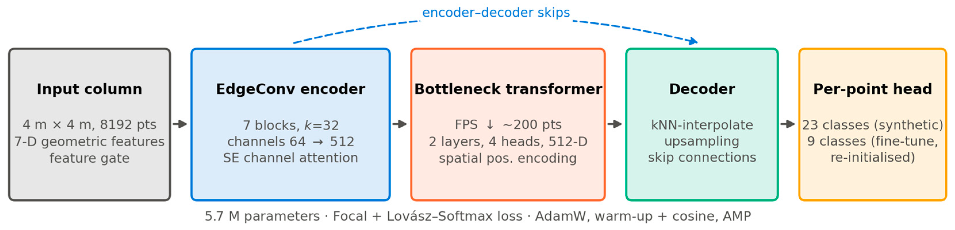
The primary network is PointEdgeSegNet [25], a lightweight EdgeConv U-Net previously developed by the author (seven blocks, k = 32, squeeze-and-excitation (SE) channel attention) with a two-layer bottleneck transformer (5.7 M parameters), trained with Focal + Lovász–Softmax loss, AdamW with warm-up and cosine schedule, automatic mixed precision (AMP; PyTorch 2.11 with PyTorch Geometric 2.8), on overlapping full-height 4 m columns of 8192 points with a leakage-controlled spatial train/validation split. Input features are geometric only (normals, surface variation [26], spatial context; 7D), as a virtual scan carries no reliable radiometry. Two external baselines run under the byte-identical harness (same blocks, loss, schedule, voting, and metrics; a single architecture flag): full-resolution DGCNN [27] and a PointNet++ single-scale-grouping (SSG) variant [28] with kNN grouping. Comparisons are therefore attributable to architecture alone. Figure 3 summarises the primary architecture.

Figure 3. PointEdgeSegNet in overview: a 4 m point column passes through a gated feature embedding, an EdgeConv encoder with SE channel attention, a two-layer bottleneck transformer operating on a farthest-point-sampling (FPS)-downsampled point set, and a kNN-interpolating decoder with encoder–decoder skips; the per-point head is 23-class for synthetic training and re-initialised at 9 classes for real-data fine-tuning.

2.4. Evaluation Protocol

Evaluation takes place in three contexts, which this section describes in turn: the synthetic held-out test, zero-shot transfer to real scans, and fine-tuning on real scans. For the synthetic test, each bridge is split along its long axis (70/30), with a 3 m buffer discarded between the parts; results aggregate the test fragments of all four bridges rather than any single case study, and the same aggregation applies to every configuration.

Boundary-aware metrics are computed in every context. A point is a boundary point if a neighbour within radius r carries a different label; mIoU@boundary, mIoU@inner, their gap (boundary drop), Boundary IoU [22], and boundary F1 are reported. The radius r = 0.10 m used in all principal tables was fixed a priori, before any model was trained, as roughly twice the sampling spacing of the synthetic clouds; its sensitivity is examined by sweeping r over 0.05–0.25 m (Section 3.3).

Real zero-shot transfer uses SemanticBridge [18], a published benchmark of 20 real TLS bridges (CC-BY-4.0), acquired and annotated by its authors—no scan in this study was collected by us—with two scanner families (Leica RTC360, Leica Geosystems, Heerbrugg, Switzerland; Faro, FARO Technologies, Lake Mary, FL, USA) that provide a cross-sensor split. The four IFC source bridges and the twenty scanned bridges are different structures (unpaired); the experiment measures whether training on synthetic scans of some bridges transfers to scans of others, which is the generalisation question practitioners face.

Label spaces and projection. The synthetic clouds are labelled in our 23-class schema-traceable ontology, the benchmark in its own 9-class scheme; the two are deliberately not harmonized at generation time. Discarding label detail is always possible later, recovering it is not, and two of the paper’s contributions (the schema-traceable ontology and the complementarity analysis) depend on the finer labels existing. Comparison is made possible by an explicit projection of model predictions onto the benchmark scheme at evaluation time (Table 4), the standard practice for cross-dataset evaluation. Ontology classes with no benchmark counterpart are unscoreable rather than wrong and are reported separately as the unmapped-prediction rate; the context classes ground/vegetation (no IFC source) are excluded from zero-shot scoring. Both policies raise the reported score and are therefore stated wherever scores appear. One semantic nuance is visible in the qualitative results of Section 3.4: the benchmark’s top surface class concentrates on at-grade trafficked surfaces (approaches), while the upper face of the bridge deck itself is labelled superstructure; the deck→top-surface projection is therefore conservative for zero-shot scoring, identically across all configurations. Because the mapping is applied to predictions of every configuration identically, plausible alternative choices for this one ambiguous pair (scoring deck as superstructure or excluding deck-top points) would shift all six absolute scores in the same direction without affecting the between-configuration contrasts that carry the paper’s conclusions; the remaining mappings of Table 4 are one-to-one at the component-family level and offer no comparable ambiguity. The fine-tuning experiment (described below) requires no projection: its 9-class head is trained and evaluated natively in the benchmark’s label space. On real data, the boundary set is derived from label transitions, and its radius sensitivity is reported.

The fine-tuning experiment runs three arms × three seeds under an identical 20-epoch budget on the benchmark’s own train split (15 bridges), evaluated on its validation split (5 unseen bridges): training from scratch and fine-tuning from backbones pre-trained on the uniform and full-realism synthetic sets (shape-matched tensor transfer; the 23→9-class head is re-initialised).

Statistical protocol. The unit of every hypothesis test in this paper is one training run (one random seed); observations are independent, not paired, with n = 3 runs per condition unless stated otherwise. Group summaries are mean ± sd over seeds. Two-group comparisons use the two-sided Welch t-test with Welch–Satterthwaite degrees of freedom, evaluated on the t distribution, and the small-sample-corrected Hedges’ g; exact t, degrees of freedom, p, and g are reported with each comparison. With n = 3 per group, these tests have low power, so effect sizes and the consistency of directions across metrics carry part of the evidential weight, and all seed-level values are given in Appendix B for reanalysis.

3. Results

3.1. Synthetic-Test Evaluation Rewards the Wrong Generator

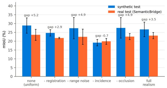
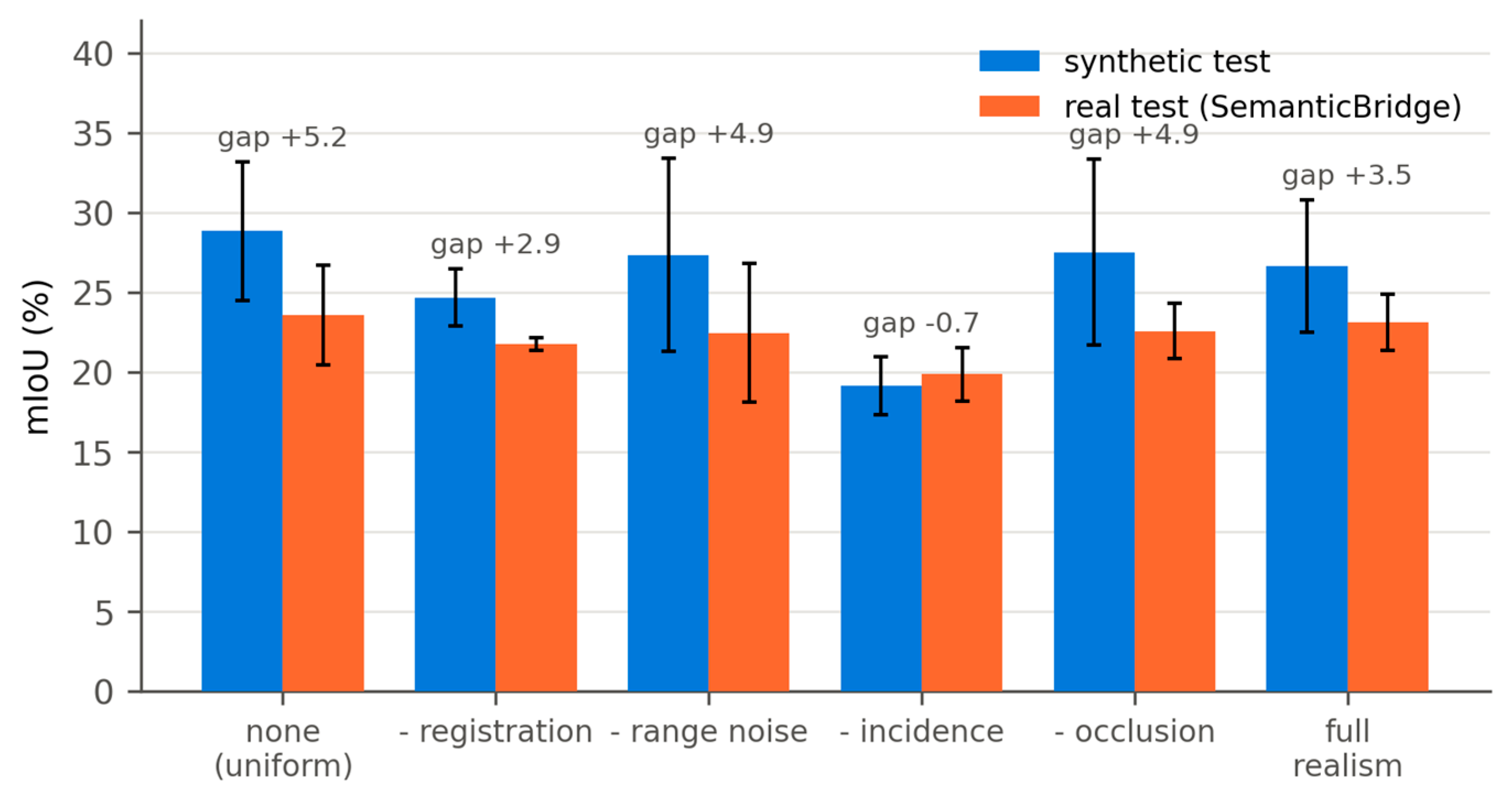
On each configuration’s own held-out synthetic split, the least realistic generator wins (Table 5): uniform sampling reaches 28.8 ± 4.4 mIoU against 26.6 ± 4.2 under full realism. As descriptive contrasts, every factor except incidence-angle dropout lowers the synthetic-test score when switched on (occlusion −3.7, range noise −3.6, registration −1.6, incidence +2.6 pp, each computed over the 18 runs as the mean of runs with the factor active minus the mean of runs with it inactive; none are significant at three seeds, |g| ≤ 0.75). Because the six-cell design does not balance the factors across conditions, these on-minus-off contrasts can mix a factor’s effect with the composition of the remaining cells and are reported as screening indications, not as factorial main-effect estimates; the identifiable comparisons are the direct contrasts of each leave-one-out cell against full realism in Table 5, and interactions among the factors are not estimable from this design. The mechanism is distributional: a cloud without acquisition effects is easier to segment, and its test split is drawn from the same easy distribution. One synthetic-test contrast reaches significance: uniform sampling scores higher OA than full realism (73.6 ± 1.6 vs. 69.8 ± 1.4, g = 2.10, t(3.9) = 3.22, p = 0.034); it also shows the largest boundary drop of any cell (11.3 vs. 8.8 pp, g = 0.85), consistent in direction but not significant at three seeds (p = 0.27). In short, the screening design supports qualitative comparisons—each ablated configuration against full realism—and the on-minus-off values are screening indications only; unbiased main effects and interaction terms would require the 2⁴ full factorial.

Table 5. Synthetic-test vs. real-transfer mIoU (mean ± sd over three seeds). “Unmapped” = predictions in classes the real benchmark cannot score. Gaps are computed from unrounded values and may differ from the difference of the rounded columns by 0.1. Every cell averages three seeds; one uniform-configuration run, previously reported as unfinished, had in fact completed—its summary file failed to serialise—and its metrics were recovered from the run log (Section 3.2). Zero-shot scores in this table are computed under label projection on structural classes only and are not comparable to the natively evaluated fine-tuning scores reported in Section 3.4.

Generator	Synthetic Test	Real Test	Gap	Unmapped
uniform (no realism)	28.8 ± 4.4	23.6 ± 3.1	+5.2	9.5%
−occlusion	27.5 ± 5.8	22.6 ± 1.7	+4.9	4.7%
−range noise	27.3 ± 6.0	22.5 ± 4.3	+4.9	3.8%
−registration	24.7 ± 1.8	21.7 ± 0.4	+2.9	4.2%
−incidence	19.1 ± 1.8	19.8 ± 1.7	−0.7	3.1%
full realism	26.6 ± 4.2	23.1 ± 1.8	+3.5	4.5%

A leading − marks a leave-one-factor-out cell: the full-realism configuration with that factor disabled (same notation in Table A2).

3.2. Real Transfer: The Overstatement, Not the Ranking, Changes

Scored on the 20 real TLS bridges (structural classes only), all six configurations land within 19.8–23.6 mIoU; no factor has a significant on-minus-off contrast on zero-shot transfer (all |Δ| ≤ 1.3 pp, p ≥ 0.30).

What changes is the synthetic-to-real gap: +5.2 under uniform sampling, +3.5 under full realism, and ≈0 for the most realistic ablation cells (Figure 4); synthetic and real scores correlate only weakly across the 18 runs (Spearman ρ = +0.53; the previously unaggregated uniform-cell run is recovered as described in Table 5, and its inclusion lowers the uniform synthetic-test mean from 31.0 to 28.8 and the headline overstatement from +7.5 to +5.2 without changing any ranking or significance statement), and the unmapped-prediction rate halves under full realism (9.5%→4.5%). Acquisition realism buys an honest benchmark before it buys transfer.

Figure 4. Synthetic-test accuracy overstates real performance by an amount that depends on the acquisition model. Paired bars give synthetic-test and real-transfer mIoU (mean ± sd over three seeds) for each screening cell of Table 5; the annotation above each pair is the overstatement gap, largest (+5.2 pp) under uniform sampling and ≈0 for the most realistic cells.

Disaggregating the full-realism configuration over the twenty bridges: Per-bridge mIoU spans 10.4–34.0 (mean 23.3, sd 5.7 over bridges), i.e., between-bridge variation is the dominant variance source, roughly twice the between-seed variation. By scanner family, cross-sensor transfer differs only mildly (Faro 22.5 ± 2.6 vs. RTC360 21.0 ± 3.1 mIoU): zero-shot difficulty is dominated by the sim-to-real gap rather than the scanner family. Per-bridge values for all twenty scans are included in the released evaluation outputs; the benchmark distributes neither typology labels nor scan-distance metadata, so a finer disaggregation by those variables is not possible from the released data. Counting the context classes ground and vegetation as intersection-free (IoU = 0) instead of excluding them gives a naive nine-class average of 15.4 ± 1.2 for full realism (and 6/9 of the structural score for every other cell), which bounds from below what an all-class evaluation would report and conveys the practical size of the domain gap. Practitioners should therefore read every zero-shot score in this paper as a structural-classes-only value under label projection: it does not represent full-scene performance on a real scan that includes ground and vegetation, for which the naive nine-class average above is the more faithful guide.

3.3. Boundary Metrics: Validation and an Observed Applicability Limit

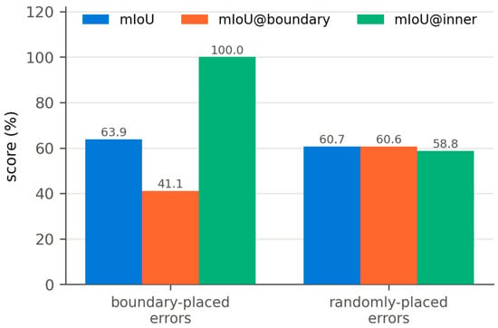
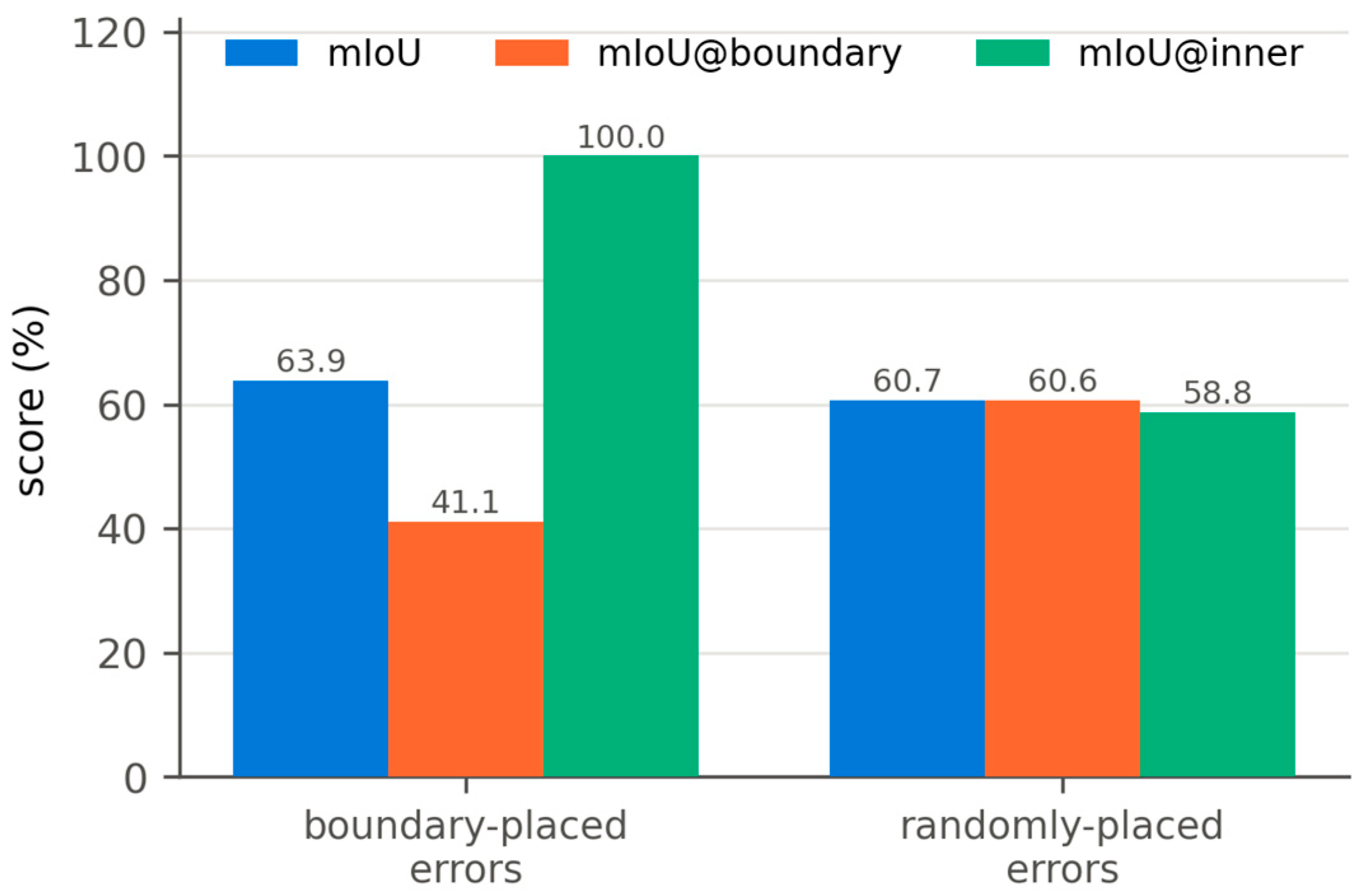
Injecting an identical number of label errors at component interfaces versus at random positions yields mIoU differing by only 3.2 points (63.9 vs. 60.7) but opposite boundary signatures (+58.9 vs. −1.9 pp drop; Figure 5). The metrics also expose their own applicability limit: under zero-shot transfer (mIoU 20–24), the boundary drop collapses to ≈0 (−3.7 to +1.3 pp); a uniformly weak model has no interface structure left to measure. Boundary quality is a meaningful axis only once the model is competent, which motivates the fine-tuning experiment. “Competent” is used here as an empirical observation, not an estimated transition point: boundary structure was measurable in every run above ~45 mIoU and in no run below ~24, and no attempt is made to locate a threshold between them.

Figure 5. Equal error counts, near-identical mIoU-boundary metrics separate the two failure modes. In the boundary-placed condition mIoU@inner is exactly 100 by construction: every injected error lies inside the boundary band, so the inner set is untouched—a check that the band isolates the injected failure mode.

The radius sensitivity of these conclusions was checked in two regimes. On the synthetic validation construction of Figure 5, the separation of the two failure modes holds at every radius in 0.05–0.25 m. On real scans, Table 6 sweeps r for the realism-pre-trained fine-tuned model on two full validation bridges: the boundary band grows from 0.2% to 7.7% of points as r grows, and the boundary drop remains large and of constant sign at every radius, so no conclusion of this paper depends on the choice of r within the swept range.

Table 6. Boundary-radius sensitivity on real data: the realism-pre-trained fine-tuned model evaluated on two unseen validation bridges (400 k-point subsamples). The boundary drop (mIoU@inner−mIoU@boundary, pp) keeps its sign and magnitude order at every radius.

r (m)	Boundary Share	Bridge A Drop	Bridge B Drop	Boundary F1 (A/B)
0.05	0.2%	+29.7	+39.7	1.5/3.4
0.10	0.9–1.3%	+29.7	+37.2	7.2/14.6
0.15	2.1–3.0%	+28.1	+34.6	19.0/28.6
0.25	5.0–7.7%	+22.8	+31.9	36.6/47.8

3.4. Fine-Tuning on Real Scans: Pre-Training and Architecture

Fine-tuning moves all arms into the competent regime (Table 7). Full-realism pre-training improves over training from scratch by +3.6 pp mIoU (50.8 ± 1.3 vs. 47.1 ± 1.3; Welch t(4.0) = 3.48, p = 0.025, corrected Hedges’ g = 2.27; seed-level tests as specified in Section 2.4, n = 3 per arm) and by +3.4 pp on mIoU@boundary (40.5 ± 1.6 vs. 37.2 ± 1.8; t(4.0) = 2.41, p = 0.074, g = 1.58)—the interface gain matches the overall gain in size and direction but does not reach significance with three seeds—whereas uniform-synthetic pre-training yields no significant gain (+0.8 pp, p = 0.64): the value of synthetic pre-training is created by acquisition realism, and the gain extends to component interfaces rather than being confined to easy interior area. Under the identical harness, full-resolution DGCNN outperforms both hierarchical models (56.5 ± 0.5 mIoU; t(2.5) = 12.2, p = 0.003 vs. scratch PointEdgeSegNet) and PointNet++ trails (46.3 ± 0.3); this is reported as measured, since no claim of this paper depends on architecture superiority, and the boundary structure (drop ≈ 9–12 pp for every competent model) is consistent across architectures. With three seeds per arm, these tests remain low-powered, so Table 7 is read jointly with effect sizes and the consistent direction of the mIoU, OA, and boundary metrics, as specified in Section 2.4. The mechanism behind the realism-pre-training gain is consistent with the distributional reading of Section 4: realistic acquisition exposes the encoder during pre-training to the geometry statistics of real scans—occlusion-shaped incompleteness, incidence-thinned surfaces, range-noise roughness—so the learned geometric features already match the fine-tuning domain, whereas uniform sampling pre-trains on implausibly complete surfaces whose features fine-tuning must first unlearn; the halved unmapped-prediction rate and the same-direction boundary gain are both consistent with this reading.

Table 7. Real-data fine-tuning, validation = five unseen bridges (mean ± sd over three seeds). Rows 2–3 initialise the PointEdgeSegNet backbone from synthetic pre-training; all other rows train from random initialisation, the two baselines under the byte-identical harness. Differences quoted in the text are computed from unrounded values and may differ from differences of the rounded entries by 0.1 pp. Evaluation is native in the benchmark’s nine-class label space with no projection and no class exclusion; values are therefore not comparable to the zero-shot scores of Table 5. Seed-level values in Table A3 of Appendix B.

Arm	mIoU	OA	mIoU@bnd	mIoU@inner
PointEdgeSegNet	47.1 ± 1.3	81.7 ± 0.9	37.2 ± 1.8	47.9 ± 1.2
+uniform pre-training	48.0 ± 2.5	81.6 ± 2.2	38.8 ± 2.5	48.7 ± 2.5
+realism pre-training	50.8 ± 1.3	83.2 ± 0.5	40.5 ± 1.6	51.6 ± 1.3
DGCNN	56.5 ± 0.5	86.9 ± 0.2	45.6 ± 0.6	57.4 ± 0.5
PointNet++	46.3 ± 0.3	76.9 ± 0.2	37.9 ± 0.5	47.0 ± 0.3

Bold marks the best of the three PointEdgeSegNet arms.

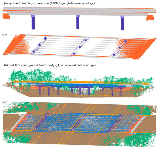
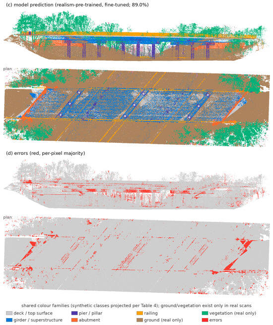
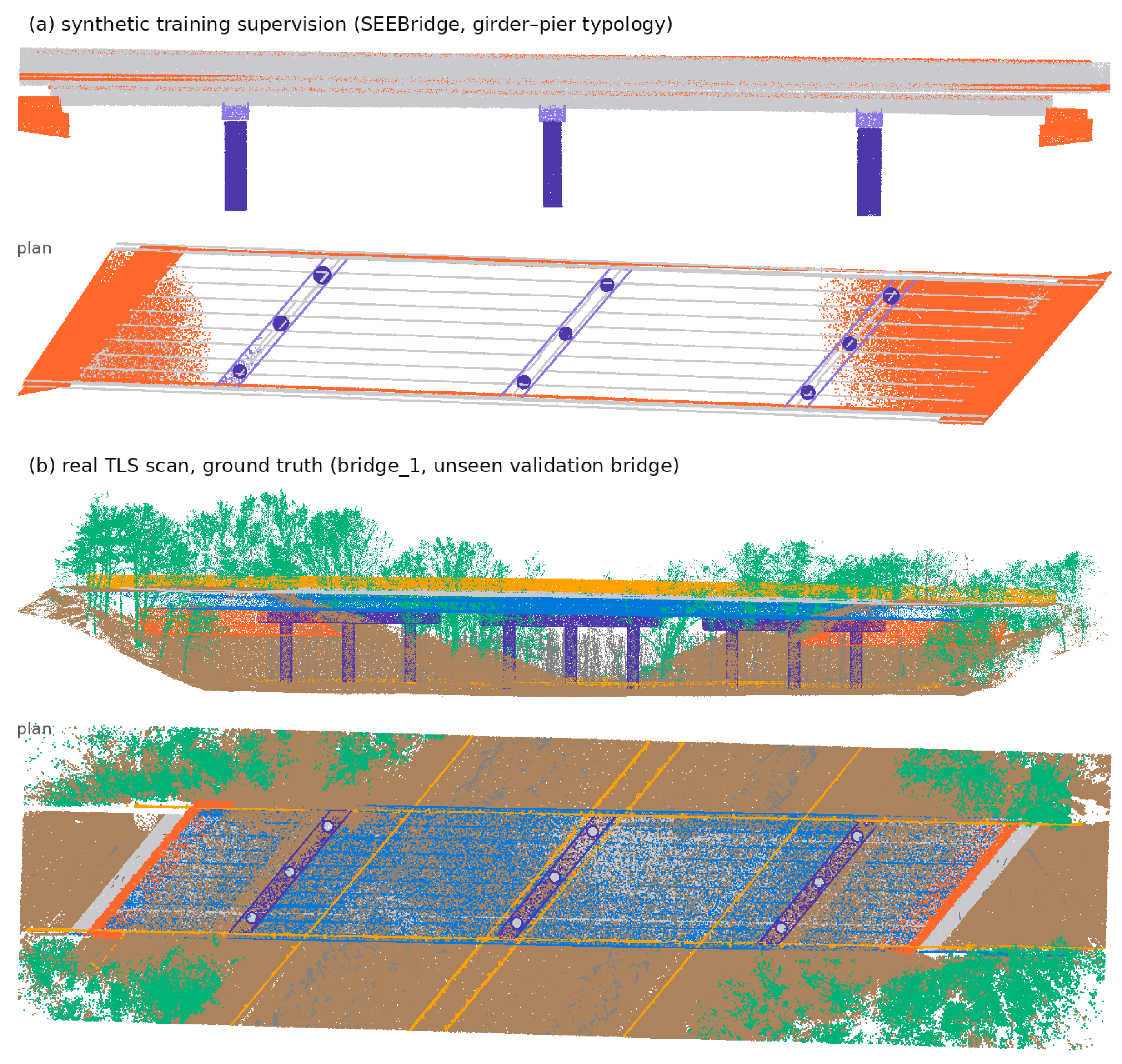
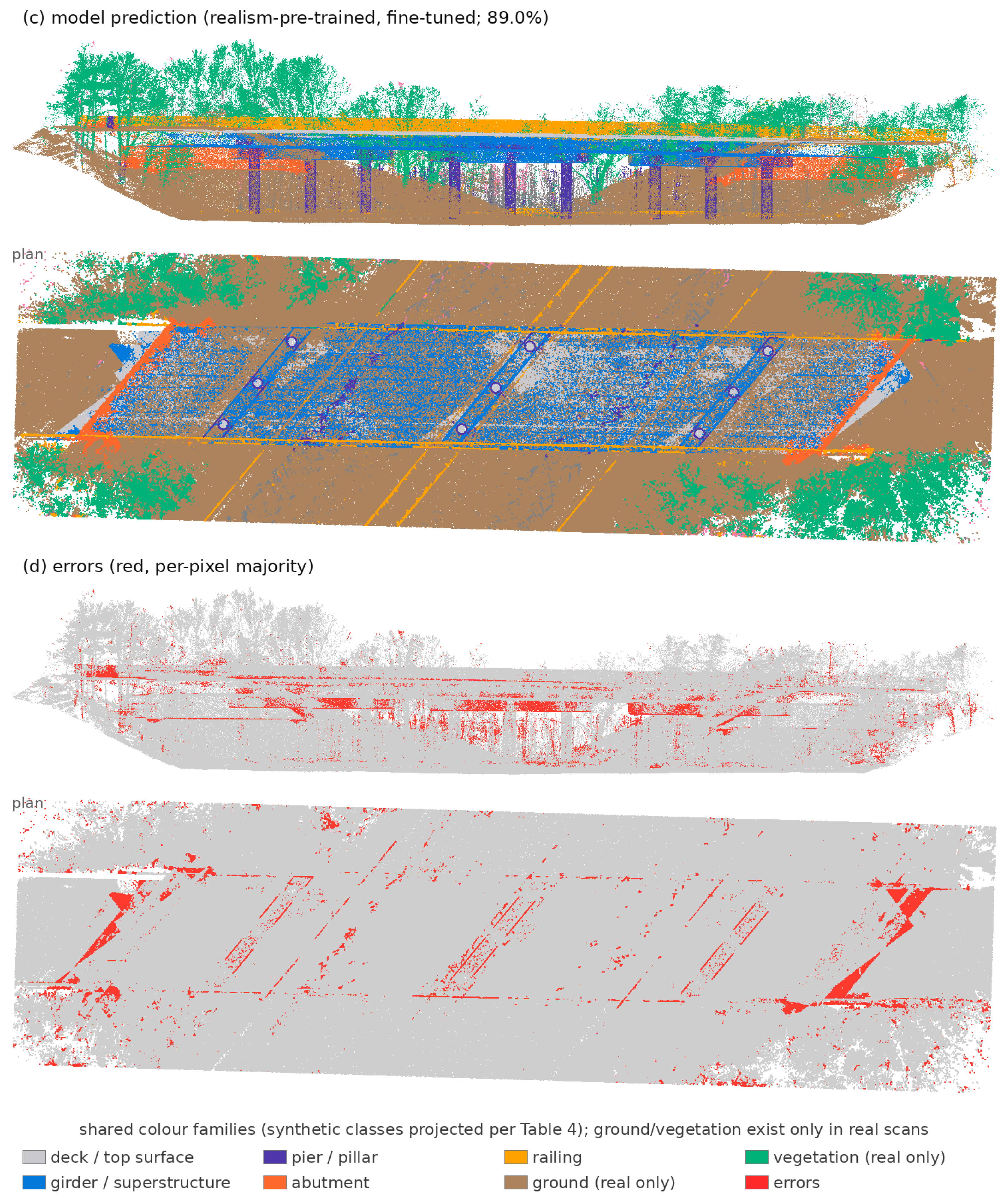
Figure 6 shows a qualitative result on an unseen validation bridge (scene accuracy 89.0%): components are recovered cleanly, and the residual errors concentrate at class boundaries and within vegetation-occluded regions-consistent with the boundary-drop statistics. Panel (a) places a synthetic training bridge of the matching typology alongside the real result in the same colour families, so the correspondence between the synthetic supervision and the real-scan prediction can be read directly within the figure.

Figure 6. From synthetic supervision to real-scan prediction, in shared colour families; each panel shows the side elevation and an axis-aligned plan view. (a) A synthetic training bridge of the matching girder–pier typology; (b) ground truth of an unseen real validation bridge (Faro scanner); (c) prediction of the realism-pre-trained fine-tuned model (scene accuracy 89.0%); (d) per-pixel-majority error map. Ground and vegetation appear only in the real scan—the complementarity of Section 3.5. In the plan view of (a) the deck interior is nearly empty: the ring of ground-level virtual stations sits ∼7 m below the deck top, so the horizontal top face is self-occluded, and only 1.4% of deck returns lie within its top 30 cm—the occlusion factor made visible. Real surveys, by contrast, include on-deck stations, which is why the real panels (b–d) show dense deck tops.

3.5. Complementarity of the Two Supervision Sources

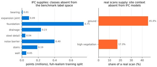
Eight of 23 ontology classes—bearing, expansion joint, foundation, drainage, noise barrier, steel detail, stairs, generic wall—have no counterpart in the real benchmark, and the IFC models supervise 0.01–0.75 million points of each at zero annotation cost. Three senses of “absent” should be distinguished here. Some of these classes are genuinely hard to observe or annotate in TLS data—bearings and expansion joints are small and frequently occluded, foundations are buried—but absence from the benchmark’s taxonomy is in the first instance a property of that label-space design, not proof that annotation is impracticable. What the data support is the label-space statement: whatever the reason for their absence, these classes receive point supervision from the IFC source that the real benchmark does not provide. Conversely, ground (45.4% of the real fine-tuning set) and high vegetation (17.3%) have no source in an IFC model (Figure 7).

Figure 7. What each supervision source uniquely provides. Left: the eight ontology classes with no benchmark counterpart and the point supervision (millions of points) the IFC models supply for them at zero annotation cost. Right: the share of the real fine-tuning set occupied by the context classes ground and high vegetation, which have no source in an IFC model.

4. Discussion

The findings carry two messages for practitioners who generate synthetic TLS training data. When a synthetic dataset will be used to rank or select anything—architectures, generators, hyper-parameters—the results indicate that acquisition realism matters for the honesty of that selection: under the acquisition magnitudes studied here, a benchmark without realism overstated real performance by up to 5.2 mIoU points and ranked the least-transferring configuration first, and reproducing the acquisition effects drove that overstatement towards zero. When the synthetic set instead serves as pre-training mass before real fine-tuning, the fine-tuning arm indicates that the realism investment still pays: only the realism-pre-trained backbone improved significantly over training from scratch, with an interface gain of the same size and direction as the overall gain. These are statements about the configurations and magnitudes investigated, not a universal claim; a differently parameterised scanner model could shift the sizes of the effects.

For evaluation practice, the two additions proposed here are nearly free. Area-dominated metrics cannot distinguish a model that fails at component interfaces from one that fails diffusely, as the validation construction of Section 3.3 shows with two error patterns of near-identical mIoU and opposite boundary signatures; reporting mIoU@boundary alongside mIoU adds one evaluation pass. Likewise, a synthetic-test score alone conceals the transfer gap; reporting the gap requires only that real evaluation data exist at all.

Why does zero-shot transfer saturate at 20–24 mIoU? Three compounding causes are visible in the data. The context classes ground and vegetation dominate real scans, have no IFC source, and absorb structural predictions; the input features are geometry-only, because a virtual scan carries no reliable radiometry; and four source bridges cannot span the typological variety of twenty real ones. Fine-tuning addresses all three at once, which is consistent with the fact that every fine-tuned arm more than doubles its zero-shot score.

The theoretical reading of the headline result is distributional. A synthetic test split drawn from the generator’s own distribution measures in-domain difficulty, not transferability; removing acquisition effects makes the distribution easier and the test split easier with it, which is why the overstatement gap, not the synthetic score, is the quantity aligned with real-world value. Acquisition realism aligns the synthetic distribution with the real one in difficulty before it measurably aligns it in transfer, and the unmapped-prediction rate—which halves under full realism—suggests that part of the alignment is semantic: realistically acquired training clouds keep predictions inside the classes a real scan can contain. The boundary axis is orthogonal to this: it separates failure modes within a fixed accuracy level, which is why it only becomes informative once accuracy is high enough for interface structure to exist.

The DGCNN result deserves a cautious reading. Under the byte-identical harness, the full-resolution baseline outperformed both hierarchical models. One hypothesis consistent with the boundary metrics is that edge features computed at full resolution retain interface detail that farthest-point-sampling pyramids blur, and that at the 4 m-column scale global context is less decisive than local relative geometry; the present experiments cannot, however, isolate the mechanism, and the statement is offered as a hypothesis for future work rather than as a demonstrated cause.

5. Limitations

Six limitations bound the scope of the conclusions. First, four source bridges are a thin basis for typological diversity: they were chosen to span four structural typologies, but many bridge forms (trusses, cable-supported systems, culverts) have no representative, and no parametric geometry variation was applied in this study—the training geometry is exactly the delivery geometry. Second, all statistics rest on three seeds per condition; the tests are correspondingly low-powered, several same-direction contrasts (notably the interface gain of realism pre-training) do not individually reach significance, and seed-level values are published in Appendix B so that the evidence can be reweighed. Third, the screening design identifies direct contrasts against full realism but not balanced main effects or interactions; a 2⁴ full factorial would be needed to estimate those. Fourth, real-data boundary ground truth is derived from label transitions rather than annotated; the radius is fixed a priori and swept (Table 6), but a transition-derived band can still differ from a surveyed interface. Fifth, the ground/vegetation exclusion raises reported zero-shot scores relative to an all-class average; the naive all-class bound is reported in Section 3.2, and the exclusion is stated wherever scores appear. Sixth, the 7.8% substantive label conflicts inherited from the delivery models are quantified (10.8% of surface area, 9.3% evaluation-relevant) but not resolved, and the synthetic-test evaluation subsamples dense columns while transfer evaluation uses coverage-guaranteed blocking, so the two synthetic-side protocols are not byte-identical. A further caveat on the boundary metrics: transition-derived bands inherit any annotation noise near interfaces—both the boundary share and mIoU@boundary then absorb labelling error, in either direction—and, as Section 3.3 shows, the metrics are informative only in the competent performance regime; outside it they should not be interpreted.

6. Conclusions

Four conclusions can be drawn from this screening study of virtual-laser-scanning realism, grounded in real IFC delivery models and validated on twenty real TLS bridge scans. First, acquisition realism did not change what a synthetic-trained model achieves on real bridges in zero-shot transfer—it changed how honestly the synthetic benchmark predicts it, shrinking a +5.2-point overstatement towards zero and halving predictions wasted on unscoreable classes; a synthetic test split should therefore not be used alone to select generators, architectures, or hyper-parameters. Second, boundary-aware metrics expose interface failures that mIoU cannot see, but only once the model is accurate enough for interface structure to exist; a regime zero-shot transfer was not reached in these experiments. Third, in the fine-tuning regime where practitioners operate, only the realism-pre-trained backbone improved significantly over training from scratch (+3.6 pp, p = 0.025, g = 2.27), with a same-direction interface gain (+3.4 pp, g = 1.58), while uniform-synthetic pre-training yielded no significant gain: the training value of BIM-derived synthetic data is created, not merely decorated, by acquisition realism. Fourth, IFC-derived and real-scan supervision are quantifiably complementary—each supplies classes the other cannot—so the two sources should be combined rather than treated as substitutes.

Future work follows directly from the limitations. A 2⁴ full factorial with more seeds would turn the screening indications into balanced main effects and interactions; parametric geometry variation (span, girder count, pier height, skew) would decouple typological diversity from the supply of delivery models; calibrating the acquisition parameters to specific instruments would connect the effect sizes to hardware choices; and annotating true interface ground truth on a small real subset would validate the transition-derived boundary bands. The full class ontology is given in Appendix A and seed-level results in Appendix B; the generation and evaluation code and the six synthetic datasets are available as described in the Data Availability Statement.

References

- Rashidi, M.; Mohammadi, M.; Sadeghlou Kivi, S.; Abdolvand, M.M.; Truong-Hong, L.; Samali, B. A decade of modern bridge monitoring using terrestrial laser scanning: Review and future directions. Remote Sens. 2020, 12, 3796. [Google Scholar] [CrossRef] [Scilit]
- Ma, J.W.; Czerniawski, T.; Leite, F. Semantic segmentation of point clouds of building interiors with deep learning: Augmenting training datasets with synthetic BIM-based point clouds. Autom. Constr. 2020, 113, 103144. [Google Scholar] [CrossRef] [Scilit]
- Griffiths, D.; Boehm, J. SynthCity: A large-scale synthetic point cloud. arXiv 2019, arXiv:1907.04758. [Google Scholar]
- Noichl, F.; Collins, F.C.; Braun, A.; Borrmann, A. Enhancing point cloud semantic segmentation in the data-scarce domain of industrial plants through synthetic data. Comput.-Aided Civ. Infrastruct. Eng. 2024, 39, 2503–2519. [Google Scholar] [CrossRef] [Scilit]
- Kellner, M.; König, T.; Jäkel, J.-I.; Klemt-Albert, K.; Reiterer, A. 3D bridge segmentation using semi-supervised domain adaptation. Autom. Constr. 2025, 172, 106021. [Google Scholar] [CrossRef] [Scilit]
- Lamas, D.; Justo, A.; Soilán, M.; Riveiro, B. Automated production of synthetic point clouds of truss bridges for semantic and instance segmentation using deep learning models. Autom. Constr. 2024, 158, 105176. [Google Scholar] [CrossRef] [Scilit]
- Yang, X.; del Rey Castillo, E.; Zou, Y.; Wotherspoon, L. Semantic segmentation of bridge point clouds with a synthetic data augmentation strategy and graph-structured deep metric learning. Autom. Constr. 2023, 150, 104838. [Google Scholar] [CrossRef] [Scilit]
- Kim, Y.; Kim, J.; Kim, J.; Kim, H. Superpoint transformer-based bridge component recognition using UAV-mounted LiDAR and synthetic point cloud generation. J. Comput. Civ. Eng. 2025, 39, 04025043. [Google Scholar] [CrossRef] [Scilit]
- Yang, X.; Fu, Y.; Kim, J. Synthetic-to-real domain adaptation with virtual laser scanning and self-training-based category-aware cuboid mixing for semantic segmentation of bridge point clouds. J. Comput. Civ. Eng. 2026, 40, 04025148. [Google Scholar] [CrossRef] [Scilit]
- Rahman, A.U.; Hoskere, V. Instance segmentation of reinforced concrete bridge point clouds with transformers trained exclusively on synthetic data. Autom. Constr. 2025, 173, 106067. [Google Scholar] [CrossRef] [Scilit]
- Winiwarter, L.; Esmorís Pena, A.M.; Weiser, H.; Anders, K.; Martínez Sánchez, J.; Searle, M.; Höfle, B. Virtual laser scanning with HELIOS++: A novel take on ray tracing-based simulation of topographic full-waveform 3D laser scanning. Remote Sens. Environ. 2022, 269, 112772. [Google Scholar] [CrossRef] [Scilit]
- Soudarissanane, S.; Lindenbergh, R.; Menenti, M.; Teunissen, P. Scanning geometry: Influencing factor on the quality of terrestrial laser scanning points. ISPRS J. Photogramm. Remote Sens. 2011, 66, 389–399. [Google Scholar] [CrossRef] [Scilit]
- Bryson, M.; Wang, F.; Allworth, J. Using synthetic tree data in deep learning-based tree segmentation using LiDAR point clouds. Remote Sens. 2023, 15, 2380. [Google Scholar] [CrossRef] [Scilit]
- Moss, C.; Letizia, S.; Iungo, G.V.; Moriarty, P.J. Realistic noise generation to enhance realism of virtual lidar scans. Remote Sens. 2025, 17, 2965. [Google Scholar] [CrossRef] [Scilit]
- Pepe, M.; Garofalo, A.R.; Costantino, D.; Tana, F.F.; Palumbo, D.; Alfio, V.S.; Spacone, E. From point cloud to BIM: A new method based on efficient point cloud simplification by geometric feature analysis and building parametric objects in Rhinoceros/Grasshopper software. Remote Sens. 2024, 16, 1630. [Google Scholar] [CrossRef] [Scilit]
- Lu, R.; Brilakis, I.; Middleton, C.R. Detection of structural components in point clouds of existing RC bridges. Comput.-Aided Civ. Infrastruct. Eng. 2019, 34, 191–212. [Google Scholar] [CrossRef] [Scilit]
- Zhang, H.; Zhu, Y.; Xiong, W.; Cai, C.S. A bridge point cloud databank for digital bridge understanding. Comput.-Aided Civ. Infrastruct. Eng. 2025, 40, 1253–1271. [Google Scholar] [CrossRef] [Scilit]
- Kellner, M.; Ferrandon Cervantes, M.; Pan, Y.; Lu, R.; Brilakis, I.; Reiterer, A. SemanticBridge-A dataset for 3D semantic segmentation of bridges and domain gap analysis. Dev. Built Environ. 2026, 26, 100912. [Google Scholar] [CrossRef] [Scilit]
- Zhou, S.; Lin, J.-R.; Pan, P.; Pan, Y.; Brilakis, I. Impact of color and mixing proportion of synthetic point clouds on semantic segmentation. Autom. Constr. 2025, 171, 105963. [Google Scholar] [CrossRef] [Scilit]
- Hu, Z.; Zhen, M.; Bai, X.; Fu, H.; Tai, C.-L. JSENet: Joint semantic segmentation and edge detection network for 3D point clouds. In Proceedings of the ECCV, Virtual, 23–28 August 2020; Springer: Cham, Switzerland, 2020; pp. 222–239. [Google Scholar]
- Tang, L.; Zhan, Y.; Chen, Z.; Yu, B.; Tao, D. Contrastive boundary learning for point cloud segmentation. In Proceedings of the IEEE/CVF CVPR, New Orleans, LA, USA, 18–24 June 2022; IEEE Computer Society: Washington, DC, USA, 2022; pp. 8489–8499. [Google Scholar]
- Cheng, B.; Girshick, R.; Dollár, P.; Berg, A.C.; Kirillov, A. Boundary IoU: Improving object-centric image segmentation evaluation. In Proceedings of the IEEE/CVF CVPR, Nashville, TN, USA, 20–25 June 2021; IEEE Computer Society: Washington, DC, USA, 2021; pp. 15334–15342. [Google Scholar]
- Chen, Y.; Xia, J.; Zou, X.; Xiao, Z.; Tang, X.; Zang, Y.; Chen, D.; Shen, Y. Contextual boundary-aware network for semantic segmentation of complex land transportation point cloud scenes. ISPRS J. Photogramm. Remote Sens. 2025, 230, 18–31. [Google Scholar] [CrossRef] [Scilit]
- Jing, Y.; Sheil, B.; Acikgoz, S. A lightweight transformer-based neural network for large-scale masonry arch bridge point cloud segmentation. Comput.-Aided Civ. Infrastruct. Eng. 2024, 39, 2427–2438. [Google Scholar] [CrossRef] [Scilit]
- Kang, T. PointEdgeSegNet: A Lightweight EdgeConv–U-Net Model for Large-Scale Point Cloud Segmentation. GitHub repository. 2025. Available online: https://github.com/mac999/point_edge_seg_net (accessed on 4 August 2026).
- Pauly, M.; Gross, M.; Kobbelt, L.P. Efficient simplification of point-sampled surfaces. In Proceedings of the IEEE Visualization, Boston, MA, USA, 27 October–1 November 2002; IEEE Computer Society: Washington, DC, USA, 2002; pp. 163–170. [Google Scholar]
- Wang, Y.; Sun, Y.; Liu, Z.; Sarma, S.E.; Bronstein, M.M.; Solomon, J.M. Dynamic graph CNN for learning on point clouds. ACM Trans. Graph. 2019, 38, 146. [Google Scholar] [CrossRef] [Scilit]
- Qi, C.R.; Yi, L.; Su, H.; Guibas, L.J. PointNet++: Deep hierarchical feature learning on point sets in a metric space. In Proceedings of the NeurIPS, Long Beach, CA, USA, 4–9 December 2017; Neural Information Processing Systems Foundation, Inc.: San Diego, CA, USA, 2017; pp. 5099–5108. [Google Scholar]
Disclaimer/Publisher’s Note: The statements, opinions and data contained in all publications are solely those of the individual author(s) and contributor(s) and not of MDPI and/or the editor(s). MDPI and/or the editor(s) disclaim responsibility for any injury to people or property resulting from any ideas, methods, instructions or products referred to in the content. |
© 2026 by the author. Licensee MDPI, Basel, Switzerland. This article is an open access article distributed under the terms and conditions of the Creative Commons Attribution (CC BY) license.