Dual Category-Guided Spatial Mamba Network for Remote Sensing Semantic Segmentation

Highlights

• What are the main findings?

• DGSMNet combines dual category guidance with spatial Mamba modeling to improve remote sensing semantic segmentation on the evaluated class-imbalanced benchmarks.

• The proposed DSCG and SPM modules improve class-specific representation, long-range context modeling, and object-boundary preservation on the Vaihingen and Potsdam datasets.

• What are the implications of the main findings?

• Explicit category guidance and spatially aware state-space modeling provide a practical strategy for improving fine-grained urban remote sensing segmentation.

• The framework can support more reliable recognition of small and visually similar urban land-cover classes.

Abstract

With the rapid development of aerospace technology, remote sensing images contain increasingly rich feature information, while large variations in object scales and imbalanced category distributions pose great challenges to remote sensing semantic segmentation. Current mainstream methods often rely on attention mechanisms for global modeling, yet they tend to over-average features, making it difficult to capture minority categories and preserve fine-grained details. To address these limitations, we propose a Dual Category-Guided Spatial Mamba Network (DGSMNet) that combines dual category guidance with a spatial Mamba mechanism. Specifically, a Dual-Stage Category Guidance (DSCG) module is designed to extract class information via wavelet transforms and guide feature learning, ensuring proportional representation of all categories across channels and enabling the model to learn underrepresented classes. In addition, a Spatial Mamba (SPM) module is introduced to enhance long-range modeling while retaining sensitivity to local details. By integrating DSCG and SPM, the proposed DGSMNet improves category-aware representation and spatial modeling on the evaluated benchmarks. Extensive experiments on the ISPRS Vaihingen and Potsdam datasets demonstrate that DGSMNet achieves competitive performance among the compared methods.

1. Introduction

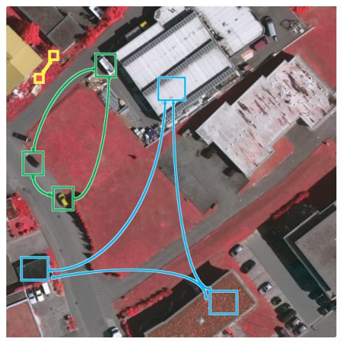
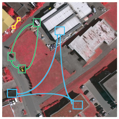
Semantic remote sensing segmentation is one of the fundamental tasks in image processing and its primary goal is to assign a class label to each pixel. Remote sensing segmentation has been widely applied to scenarios such as road extraction [1], disaster monitoring [2], land-cover classification [3], and urban planning [4]. As the spatial resolution and information content of remote sensing imagery increase, traditional machine-learning methods such as support vector machines (SVMs) [5] face difficulties in segmentation because handcrafted features are tedious to design and insufficient for fine-grained pixel-wise discrimination. Meanwhile, numerous issues remain in remote sensing semantic segmentation. As shown in Figure 1, objects of the same semantic class, such as buildings and cars, can exhibit substantial intra-class variation, while different classes such as trees and low vegetation can show strong inter-class appearance similarity. Moreover, cars occupy an extremely small fraction of the scene. These challenges have motivated a growing body of research on category-guided approaches for remote sensing semantic segmentation.

Figure 1. Existing issues in remote sensing semantic segmentation: The models only focus on the information about major categories, while objects belonging to few-shot categories cannot be fully learned due to their extremely low proportion in the dataset. Blue denotes variations within the same building class, green shows differences in car shape and color within one class, and yellow indicates that trees and low vegetation from different classes appear visually similar.

With the rapid development of deep learning [6] and upgrades in computing hardware, deep learning-based semantic segmentation methods have been adopted for remote sensing. FCNs [7] first brought CNNs into semantic segmentation and enabled end-to-end pixel-wise training on images by replacing fully connected layers with convolutions, but the resulting feature maps are relatively coarse and lack full global context. Encoder–decoder designs such as SegNet [8] preserve edge details and spatial structure better than simple interpolation upsampling, while U-Net [9] further introduced skip connections to fuse shallow and deep features; nevertheless, effective deep–shallow fusion remains challenging. Building on these networks, the PSPNet [10] improved multi-scale context modeling for segmentation. The DeepLab series [11,12,13] introduced atrous convolutions and Atrous Spatial Pyramid Pooling (ASPP) and later used depthwise separable convolutions to cut complexity while improving multi-scale context modeling. Recent advances in remote sensing segmentation focus on multi-scale fusion and global–local collaboration. FDGSNet [14] employs frequency decomposition plus multimodal gated fusion to separate and fuse different frequency bands, boosting small-object and boundary recognition.

Nevertheless, intrinsic CNN limitations persist: a constrained receptive field, sensitivity to scale variation and very small targets. To address these shortcomings, recent works increasingly incorporate transformers to provide long-range context and dynamic, token-wise attention, enabling more effective global–local modeling and multi-scale reasoning; common designs fuse CNN encoders for fine local detail with transformer modules for global context. FTransUNet [15] fuses shallow and deep CNN features with transformer blocks to retain fine local details while aggregating global context. HGBFormer [16] integrates hypergraph-based high-order correlation modeling with a Biformer backbone plus dual pooling and feature aggregation modules to strengthen local semantic extraction within transformer reasoning. However, global–local fusion can aggravate the long-tail class imbalance endemic to remote sensing, yielding models biased toward majority classes while underrepresenting minority classes and producing marked drops in performance on those labels. Therefore, architectures must preserve high-resolution local cues for tiny objects, and explicitly counteract class imbalance so that scarce classes receive amplified, reliable attention without degrading performance on prevalent classes.

In recent years more and more researchers have turned their attention to category-guided approaches in remote sensing semantic segmentation. LoG-CAN [17] proposes a global class-aware module and local class-aware modules to capture class-wise global context and local class representations. CGGLNet [18] uses category information to steer both global contextual modeling and local feature interaction.

Motivated by these observations, we propose a Dual Category-Guided Spatial Mamba Network (DGSMNet) that consists of two principal modules: a Dual-Stage Category Guidance (DSCG) module and a Spatial Mamba (SPM) module. The DSCG itself comprises a Wavelet Guidance Module (WGM) and a Fusion Guidance Module (FGM): WGM uses discrete wavelet transforms to extract multi-scale texture and contour cues for each class to enhance minority class representations [19,20], while FGM refines per-class proportions across spatial and channel dimensions to ensure minority classes receive sufficient representational capacity. The SPM employs a Mamba-style global–local modeling mechanism that injects explicit spatial cues to preserve object structure and fine details while enabling long-range context aggregation. Together, DSCG and SPM help the network attend to rare classes under severe imbalance while capturing spatially aware long-range dependencies. We evaluate DGSMNet on the ISPRS Vaihingen and Potsdam benchmarks and report extensive comparisons and ablation studies to validate the effectiveness of the proposed approach. The contributions of this work are summarized in three aspects as follows:

(1)

We propose a novel semantic segmentation network, Dual Category-Guided Spatial Mamba Network (DGSMNet), which guides the model to attend to all class information via class-aware guidance to mitigate class imbalance. Simultaneously, DGSMNet employs a Mamba scanning mechanism combined with spatial extraction to complement global context, thereby improving segmentation accuracy.

(2)

We introduce a Dual-Stage Category Guidance (DSCG) module, which is composed of a Wavelet Guidance Module WGM followed by a Fusion Guidance Module FGM. DSCG efficiently extracts class-specific cues and ensures that class information maintains appropriate proportions across spatial and channel dimensions so that all classes receive sufficient attention. In particular, WGM performs wavelet-based guidance to extract frequency-domain multi-scale texture and contour features that enhance per-sample representations, while FGM adjusts per-class channel proportions on the classified feature maps and further guides features to guarantee comprehensive attention to every class.

(3)

We propose a Spatial Mamba module (SPM), where the Mamba mechanism models long-range dependencies using a one-dimensional sequence formulation to enable cooperation between global semantics and local details. A dedicated spatial branch focuses on multi-scale local textures and edge features to strengthen the network’s sensitivity to complex spatial structures, thereby improving the segmentation accuracy of object boundaries and small targets in remote sensing images.

The remainder of this paper is organized as follows. Section 2 reviews related work. Section 3 presents the overall architecture of DGSMNet, the DSCG and SPM modules, and the loss functions. Section 4 describes the datasets and experimental settings. Section 5 reports the comparative and ablation results. Section 6 discusses category guidance, model efficiency, and limitations. Finally, Section 7 concludes the paper.

2. Related Work

2.1. Single-Modal Semantic Segmentation

FCN [7] introduced an end-to-end, pixel-wise learning paradigm that enabled direct dense prediction, but its limited receptive field and coarse object boundaries remain problematic. Encoder–decoder designs such as U-Net [9] and SegNet [8] partly alleviate these issues by aggregating multi-scale features through progressive downsampling and by using index-guided upsampling, respectively. More recently, UNetFormer [21] integrates transformer-based modules into the U-Net paradigm to better model long-range context while retaining efficient multi-scale reconstruction. Ma et al. [22] incorporate SAM-generated object and boundary constraints to refine segmentation outputs and preserve object contours, while FDNet [23] proposes a frequency decoupling network that separates and processes complementary frequency bands to better capture both fine details and global context in VHR images.

2.2. Multimodal Semantic Segmentation

With advances in remote sensing, multiple modalities such as optical (RGB), infrared, radar, and Digital Surface Model (DSM) imagery are increasingly used in practical applications, where DSM provides explicit height information and can also help delineate object boundaries. FTransUNet [15] performs multilevel modality fusion by enabling interactions between features extracted by CNNs and ViTs, while progressively integrating DSM features with RGB features to jointly preserve local details and global contextual information. LMFNet [24] is a lightweight multi-branch fusion network that employs shared-weight encoders and efficient cross-attention fusion layers to combine RGB, NIR and DSM with minimal parameter overhead; TMFNet [25] uses a transformer-based multimodal fusion model that injects height tokens into token-level attention and uses multi-scale token merging to adaptively blend global DSM context with fine RGB details.

2.3. Category Guidance in Remote Sensing Semantic Segmentation

Remote sensing images typically contain rich features spanning many object categories. These categories are often imbalanced, not only in terms of total pixel counts but also because class proportions can vary greatly within local image regions. Consequently, an increasing number of researchers have incorporated category guidance into remote sensing semantic segmentation. CaFE [26] performs class-conditioned multimodal fusion and reweights features according to local class proportions. LoG-CAN [17] proposes a global–local class-aware network to learn class-wise global context and local class representations for robust multi-scale segmentation. SACANet [27] designs a scene-aware class attention mechanism that embeds scene context and class attention to suppress background noise while enhancing class-specific cues. CSBNet [28] develops a category-guided structural block that iteratively exchanges coarse class cues and contextual features to refine class-specific structures and reduce small-class information loss.

2.4. Mamba in Remote Sensing Semantic Segmentation

Recent state-space sequence models (SSMs) gave rise to the Mamba family, which attains linear-time global context modeling via selective state-space dynamics. Mamba introduces the selective state-space formulation for linear-time sequence modeling, laying the theoretical foundation for efficient long-range token interactions. VMamba [29] adapts the original Mamba to vision by introducing Visual State Space (VSS) blocks and 2D selective scans (SS2D), enabling efficient image-level global context aggregation while preserving spatial locality for dense prediction. RS³-Mamba [30] tailors VSS scans and lightweight decoder designs to high-resolution remote sensing dense prediction, extending scan directions and stagewise fusion to better aggregate oriented structures and process large tiled images with linear complexity. SkyMamba [31] addresses these limitations by jointly fusing visual and geometric features and leveraging state-space models for efficient long-range context modeling, achieving robust performance under class-imbalanced urban scenarios.

DGSMNet differs from these related directions in how the three operations are coupled. Category-guided methods such as CaFE, LoG-CAN, and CGGLNet refine features using class context, whereas DGSMNet assigns every WGM channel to a fixed dataset class through direct multi-scale supervision and transfers the resulting spatial prior to a corresponding channel group in FGM. Unlike frequency-aware networks that use frequency decomposition as a general feature extractor, WGM uses fixed, localized Haar subbands to generate class-specific guidance maps. In the decoder, SPM combines a four-direction 2D selective scan with explicit horizontal and vertical spatial projections at each progressive decoding scale. Thus, the technical contribution is the supervised class-to-channel guidance path and its integration with a spatially augmented state-space decoder, rather than the independent use of wavelets or Mamba.

3. Materials and Methods

In this section, we describe the architecture and constituent modules of DGSMNet. First, the Mamba framework is introduced. The overall network architecture is then presented, followed by the Dual-Stage Category Guidance (DSCG) module, including its first stage, the Wavelet Guidance Module (WGM), and its second stage, the Fusion Guidance Module (FGM). Finally, the design of the Spatial Projection Mamba and the loss functions used to update the network parameters are described.

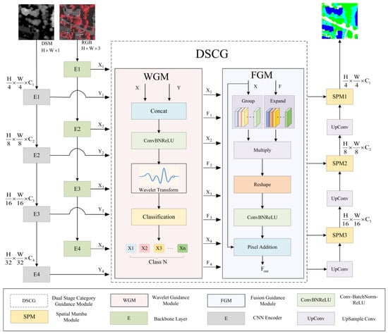
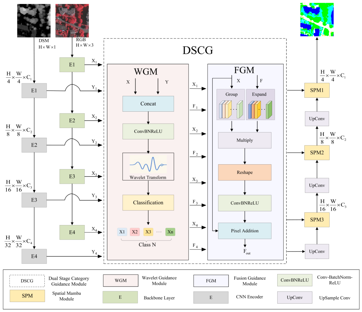
The overall network architecture of DGSMNet is shown in Figure 2.

Figure 2. The main network framework of DGSMNet. DGSMNet is a category-guided network that ensures proportional representation of class information across channels, enabling the model to learn from few-shot class samples and enhance class-specific feature learning.

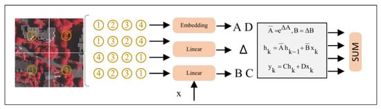
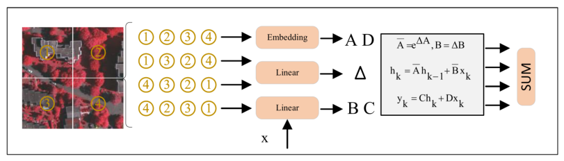
The four-direction scanning mechanism used in the SPM module is shown in Figure 3.

Figure 3. The scanning mechanism in Mamba. These four complementary paths perform state-space modeling in parallel to capture bidirectional spatial dependencies in both row and column dimensions, ensuring the characterization of full-dimensional neighborhood context for each pixel with linear computational complexity.

3.1. Preliminaries

(1) State-space models (SSMs) provide a principled framework for describing the temporal evolution of dynamical systems and have long been applied in control theory and time series modeling. In a continuous-time SSM, the dynamics map an input signal into a latent trajectory via a system of ordinary differential equations, and the latent trajectory is then projected back to produce an output sequence. Formally, this process can be written as:

$$\begin{array}{cc}\hfill h^{\prime }\left(t\right)& = Ah\left(t\right) + Bx\left(t\right)\hfill \\ \hfill y\left(t\right)& = Ch\left(t\right) + Dx\left(t\right)\hfill \end{array}$$

(1)

where $h\left(t\right) \in {\mathbb{R}}^N$ denotes the latent state, $x\left(t\right) \in {\mathbb{R}}^L$ the input, and $y\left(t\right) \in {\mathbb{R}}^L$ the output. The term $h^{\prime }\left(t\right) \in {\mathbb{R}}^N$ denotes the time derivative of the latent state. Here N and L indicate the dimensions of the latent space and the input/output sequences, respectively. The matrix $A \in {\mathbb{R}}^{N\times N}$ governs state transitions, while $B \in {\mathbb{R}}^{N\times L}$ and $C \in {\mathbb{R}}^{L\times N}$ are input and output projection matrices. The matrix D typically acts as a residual (often omitted). To deploy continuous SSMs on discrete-time data, the Mamba framework applies a zero-order hold discretization of the ODEs:

$$\begin{array}{cc}\hfill \overline{A}& = exp\left(\mathrm{\Delta }A\right),\hfill \\ \hfill \overline{B}& = {\left(\mathrm{\Delta }A\right)}^{-1}(exp\left(\mathrm{\Delta }A\right)-I)·\mathrm{\Delta }B\hfill \end{array}$$

(2)

where $\overline{A}$ and $\overline{B}$ are the discrete-time equivalents of A and B obtained with step size $\mathrm{\Delta }$. In practice, the input projection $\overline{B}$ is often approximated efficiently using a first-order Taylor expansion:

$$\overline{B}=(exp\left(A\right)-I)A^{-1}B \approx \left(\mathrm{\Delta }A\right){\left(\mathrm{\Delta }A\right)}^{-1}\mathrm{\Delta }B = \mathrm{\Delta }B,$$

(3)

After discretization, the continuous ODEs reduce to the familiar linear recurrence

$$\begin{array}{cc}\hfill h_t& = \overline{A}{h}_{t-1}+\overline{B}{x}_t,\hfill \\ \hfill y_t& = C{h}_t,\hfill \end{array}$$

(4)

where $\overline{A}$ and $\overline{B}$ denote the discrete-time state and input matrices obtained from $A, B,$$h_t$ is the latent state at discrete step t, and $x_t, y_t$ are the discrete input and output vectors respectively.

(2) Selective Scan Mechanism: Standard SSMs are linear and time-invariant: their parameter matrices are fixed and do not depend on the particular input sequence. This time invariance implies a uniform, non-selective influence over sequence positions. Specifically, the projection matrices are produced conditionally on the input $X \in {\mathbb{R}}^{B\times L\times D}$, so that $B \in {\mathbb{R}}^{B\times L\times N}$, $C \in {\mathbb{R}}^{B\times L\times N}$, and $\mathrm{\Delta } \in {\mathbb{R}}^{B\times L\times D}$ vary with the sequence. This converts the model into a linear time-varying system, enabling selective, data-dependent scanning of sequence elements and improving the model’s ability to capture complex, non-stationary temporal patterns.

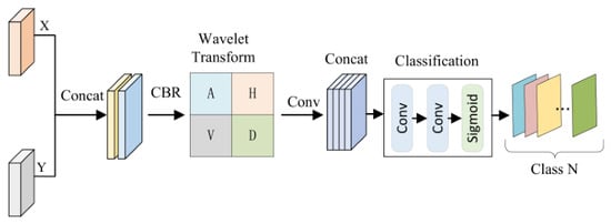
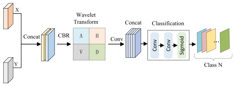
The structure of the Wavelet Guidance Module (WGM) is shown in Figure 4.

Figure 4. The structure of the Wavelet Guidance Module (WGM). WGM first extracts high- and low-frequency features through a wavelet transform to capture texture details and contour information. A convolutional classification head and a sigmoid function then produce one attention map for each semantic class. The output channels follow the dataset label order and are directly constrained by the corresponding binary class masks at every encoder stage.

3.2. Network Architecture

The overall architecture of DGSMNet is illustrated in Figure 2, adopting a classical encoder–decoder design. In the encoder, we use $DSM \in {\mathbb{R}}^{1\times H\times W}$ and $RGB \in {\mathbb{R}}^{3\times H\times W}$ images as input features, providing complementary information about object height variations and boundary cues. Here, C denotes the number of channels, and H and W represent the height and width of the input image, respectively. Specifically, the RGB branch employs a pre-trained ConvNeXt-Tiny backbone for multi-scale feature extraction, while the DSM branch is composed of lightweight CNN blocks, organized into four stages. Each stage performs downsampling by a factor of 2, producing feature maps at resolutions $H/4\times W/4$, $H/8\times W/8$, $H/16\times W/16$, and $H/32\times W/32$.

For each stage of the dual-branch encoder, a DSCG module is introduced for dual guidance. In the first stage, the WGM module generates class attention maps from the aligned fusion of DSM and RGB features to provide precise guidance for subsequent fusion. Each attention channel is assigned to a fixed semantic class according to the dataset label order and receives direct supervision from the corresponding downsampled one-hot ground-truth mask. In the second stage, the FGM module performs class-preserving channel expansion based on the prior attention map, guiding grouped RGB features stagewise to ensure each class is sufficiently represented in the feature channels. This process can be formulated as:

$$\begin{array}{cc}\hfill F_{wgm}^i& = \mathrm{WGM}\left(Concat\right(X,Y\left)\right),i = 1,2,3,4\hfill \\ \hfill F_{fgm}^i& = \mathrm{FGM}(F_{wgm}^i,X),i = 1,2,3,4\hfill \end{array}$$

(5)

where i indexes the encoder stage, X represents the RGB branch features, Y represents the DSM branch features, $WGM(·)$ is the wavelet guidance module, $FGM(·)$ is the fusion guidance module, $F_{wgm}^i$ is the supervised class attention map output by WGM, and $F_{fgm}^i$ is the class-guided feature output by FGM.

The decoder consists of three SPM modules. First, the deepest guided feature is upsampled to generate the initial decoder input. Subsequent decoder blocks integrate category-guided features from DSCG via skip connections. At each decoder stage, SPM first fuses the RGB features and the guided features, then applies the Mamba scan mechanism to capture global semantics, combined with spatial projection to extract spatial information. After processing through the three SPM stages, the final segmentation output is obtained. SPM3, SPM2, and SPM1 operate successively at $H/16\times W/16$ (384 channels), $H/8\times W/8$ (192 channels), and $H/4\times W/4$ (96 channels), respectively. The progressive decoder is formulated as:

$$\begin{array}{cc}\hfill F_{\mathrm{spm}}^4& =F_{\mathrm{fgm}}^4,\hfill \\ \hfill F_{\mathrm{spm}}^i& ={\mathrm{SPM}}_i\left(Up\left(F_{\mathrm{spm}}^{i+1}\right)+F_{\mathrm{fgm}}^i\right),i=3,2,1.\hfill \end{array}$$

(6)

where $F_{\mathrm{spm}}^4$ initializes the decoder with the deepest guided encoder feature. At each subsequent level, $Up(·)$ upsamples and projects the preceding deeper SPM output to match the channel dimension of the skip feature $F_{\mathrm{fgm}}^i$. The fused feature is then refined by ${\mathrm{SPM}}_i$ to produce $F_{\mathrm{spm}}^i$.

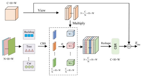
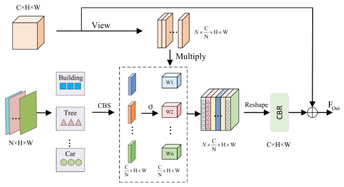
The structure of the Fusion Guidance Module (FGM) is shown in Figure 5.

Figure 5. The structure of the Fusion Guidance Module (FGM). FGM expands the attention maps obtained from WGM and multiplies them with the original features to ensure the proportional representation of each class feature across channels during training, enabling the model to focus on different class information.

3.3. Dual-Stage Category Guidance

(1) Wavelet Guidance Module: In general image segmentation networks, the model learns from all information jointly and only reconciles class-wise predictions at the output stage. For tasks with many and imbalanced classes, such global learning tends to bias the model toward classes with larger sample proportions, while underrepresented classes lack sufficient feature capacity and parameters for reliable modeling. Reducing inter-class competition during learning and ensuring enough representational space for every class is therefore crucial for balancing segmentation performance on imbalanced remote sensing data.

To address this issue, we design a Wavelet Guidance Module (WGM) to obtain class-aware attention maps that serve as priors for subsequent guided fusion, as illustrated in Figure 4. The module first fuses and aligns RGB encoder features X and DSM encoder features Y by channel-wise concatenation and a convolutional alignment block, thereby injecting height and contour cues into the network. The fused feature is computed as:

$$F_{\mathrm{fuse}}^i=\mathrm{ConvBNReLU}\left(\mathrm{Concat}(X_i,Y_i)\right),i=1,2,3,4,$$

(7)

where $X^i$ and $Y^i$ denote the features from the RGB and DSM encoder branches at stage i, respectively; $\mathrm{Concat}(·)$ is channel concatenation; and $\mathrm{ConvBNReLU}(·)$ denotes a convolutional block followed by batch normalization and ReLU activation.

Next, a one-level 2D discrete wavelet transform is applied per channel to decompose $F_{\mathrm{fuse}}$ into spatially localized approximation and detail subbands. For a single-channel feature map $S_c$, let $s_{pq}=S_c(2i-1+p,2j-1+q)$, where $p,q\in \{0,1\}$. The Haar coefficients of each non-overlapping $2\times 2$ block are:

$$\begin{array}{cc}\hfill A_c(i,j)& ={\displaystyle \frac{s_{00}+s_{01}+s_{10}+s_{11}}{2}},\hfill \\ \hfill H_c(i,j)& ={\displaystyle \frac{s_{00}-s_{01}+s_{10}-s_{11}}{2}},\hfill \\ \hfill V_c(i,j)& ={\displaystyle \frac{s_{00}+s_{01}-s_{10}-s_{11}}{2}},\hfill \\ \hfill D_c(i,j)& ={\displaystyle \frac{s_{00}-s_{01}-s_{10}+s_{11}}{2}}.\hfill \end{array}$$

(8)

where the approximation subband $A_c$ retains coarse region extent and stable RGB–DSM structure, whereas $H_c$, $V_c$, and $D_c$ preserve directional boundaries and local textures. Their combination supplies region support for large classes while retaining fine transitions and compact objects, allowing the class head to learn a category-dependent mixture of structural and detail cues. Unlike the global frequency representation of FFT, the wavelet coefficients remain associated with local spatial regions and are therefore suitable for dense class guidance. The indices satisfy $i=1,\dots ,H/2$ and $j=1,\dots ,W/2$.

We concatenate the four subbands across the channel dimension to form the frequency-domain feature:

$$F_f=\mathrm{Concat}(A,H,V,D),$$

(9)

where $A, H, V, D$ collect the per-channel coefficients $\left\{A_c\right\}, \left\{H_c\right\}, \left\{V_c\right\}, \left\{D_c\right\}$, respectively. For an input $F_{\mathrm{fuse}}^i \in {\mathbb{R}}^{C_i\times H_i\times W_i}$, each subband has size $C_i\times H_i/2\times W_i/2$, and $F_f^i \in {\mathbb{R}}^{4C_i\times H_i/2\times W_i/2}$. The one-level Haar transform is fixed and parameter-free; only the subsequent depthwise and pointwise convolutions are learned.

Finally, a convolutional classification head maps $F_f^i$ to N channel logits $Z_{\mathrm{wgm}}^i$, and a sigmoid activation produces the class attention maps $A_{\mathrm{wgm}}^i$:

$$\begin{array}{cc}\hfill Z_{\mathrm{wgm}}^i& = {\mathrm{Conv}}_{1\times 1}\left({\mathrm{Conv}}_{3\times 3}\left(F_f^i\right)\right),\hfill \\ \hfill A_{\mathrm{wgm}}^i& = \sigma \left(Z_{\mathrm{wgm}}^i\right),A_{\mathrm{wgm}}^i\in {[0,1]}^{N\times H_i\times W_i}.\hfill \end{array}$$

(10)

where ${\mathrm{Conv}}_{1\times 1}(·)$ and ${\mathrm{Conv}}_{3\times 3}(·)$ denote $1\times 1$ and $3\times 3$ convolutions, respectively, and $\sigma (·)$ is the sigmoid function. The channel order is fixed to the dataset label order; that is, channel n represents semantic class n at every scale. To establish this correspondence explicitly rather than relying on an emergent ordering, the one-hot ground-truth mask is resized to $(H_i, W_i)$ by nearest-neighbor interpolation, producing $Y^i \in {\{0,1\}}^{N\times H_i\times W_i}$. We impose a channel-wise class-alignment loss at each encoder stage:

$${\mathcal{L}}_{\mathrm{align}}^i=-{\displaystyle \frac{1}{N|{\mathsf{\Omega }}_i|}}{\displaystyle {\sum }_{n=1}^N}{\sum }_{p\in {\mathsf{\Omega }}_i}\left[Y_n^i\left(p\right)log{A}_{\mathrm{wgm},n}^i\left(p\right)+\left(1-Y_n^i\left(p\right)\right)log\left(1-A_{\mathrm{wgm},n}^i\left(p\right)\right)\right],$$

(11)

where ${\mathsf{\Omega }}_i$ is the spatial domain at stage i. Consequently, permuting two WGM channels changes the alignment loss because each channel is compared only with its designated semantic mask. This direct multi-scale supervision therefore establishes an identifiable channel-to-category correspondence throughout training.

(2) Fusion Guidance Module: Since the WGM focuses on spatially localizing class priors, it provides spatial guidance that helps the network preserve spatial priors while enhancing class-discriminative cues and supplying more precise guidance for the decoder. Building upon this spatial prior, we design the Fusion Guidance Module (FGM) to concentrate on channel-wise feature alignment and expansion. Given the attention maps produced by WGM, FGM independently expands each class map into $C/N$ channels using a class-preserving grouped $1\times 1$ projection. The RGB features are divided into N groups in the same fixed class order, and group n is modulated only by the expanded map originating from WGM channel n. No cross-class mixing is introduced before this modulation. A Conv–BatchNorm–ReLU (CBR) block then captures cross-channel semantics after the class-wise modulation, and a residual connection adds the enhanced feature back to the original RGB feature. This procedure is formulated as:

$$\begin{array}{cc}\hfill F_{\mathrm{expand}}& = {\mathrm{CBS}}_{\mathrm{group}}\left(F_{\mathrm{wgm}}\right),\hfill \\ \hfill F_{\mathrm{group}}& = R_1\left(X\right),\hfill \\ \hfill F_{\mathrm{fgm}}& = \mathrm{CBR}\left(R_1^{-1}(F_{\mathrm{expand}}\odot F_{\mathrm{group}})\right)+X,\hfill \end{array}$$

(12)

where $F_{\mathrm{expand}}$ denotes the channel-expanded attention, $F_{\mathrm{group}}$ is the RGB feature after channel-wise grouping, and $F_{\mathrm{fgm}}$ is the category-guided reconstructed feature. ${\mathrm{CBS}}_{\mathrm{group}}$ denotes the class-preserving grouped $1\times 1$ projection followed by batch normalization and sigmoid activation. ⊙ denotes element-wise multiplication, and $\mathrm{CBR}(·)$ denotes a Conv–BatchNorm–ReLU block. The reshape operator $R_1$ maps a tensor of shape ${\mathbb{R}}^{C\times H\times W}$ to ${\mathbb{R}}^{N\times (C/N)\times H\times W}$, and $R_1^{-1}$ restores the grouped tensor back to ${\mathbb{R}}^{C\times H\times W}$. In both datasets, $N=6$ in the fixed order: impervious surface, building, low vegetation, tree, car, and clutter/background; clutter therefore participates in WGM guidance and FGM grouping during training. The encoder widths $C_i=96,192,384,768$ are divisible by six, giving $C_i/N=16,32,64,128$ channels per class group at the four stages.

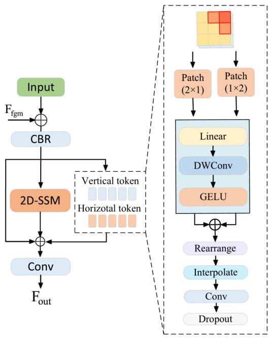
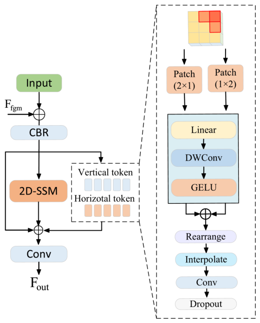
The structure of the Spatial Mamba Module (SPM) is shown in Figure 6.

Figure 6. The structure of the Spatial Mamba Module (SPM). SPM extracts horizontal and vertical feature sequences and then fuses them to enable the network to capture spatial information.

3.4. Spatial Mamba Module

Global and local information are both crucial for remote sensing semantic segmentation: global context helps the model capture long-range dependencies and scene-level layouts, while local cues focus on neighborhood textures, edges and shape details that are essential for accurate segmentation of small objects and precise boundary localization.

Inspired by linear-complexity visual Mamba models such as VMamba, we design SPM for the decoder. Given an input feature tensor $X \in {\mathbb{R}}^{B\times C\times H\times W}$, SPM first applies convolutional upsampling to channels and then adds the skip-connected fusion-guided feature from FGM to obtain a class-guided decoder input, which is further processed through a CBR module. The processing then splits into two parallel branches: one branch passes features through a 2D-SSM block to extract local and long-range spatial cues; in parallel, an auxiliary spatial branch reshapes the input into vertical and horizontal sequences via $2\times 1$ and $1\times 2$ patching, respectively. The 2D-SSM uses four scan directions with state dimension 16, depthwise-convolution kernel size 3, expansion ratio 2, and $dt$ rank $\lceil C/16\rceil$. Specifically, the vertical branch splits the input into $(H/2)\times W$ non-overlapping patches, forming a tensor of shape $B\times \left(\right(H/2)\times W)\times 2C$ and projects it to $B\times \left[\right(H/2)\times W]\times \dim$ via a linear layer, while the horizontal branch splits the input into $H\times (W/2)$ patches, resulting in a tensor of $B\times (H\times (W/2\left)\right)\times 2C$ and projects it to $B\times (H\times (W/2\left)\right)\times \dim$ through the same linear projection. Afterward, the processed sequences from the auxiliary branch are reshaped back to $B\times C\times H\times W$, and the outputs of the two parallel branches are summed element-wise to form the final decoded feature.

Finally, the main branch 2D-SSM output and the auxiliary spatial output are combined, passed through a convolution and dropout, and added to produce the decoder block output. This pipeline is compactly expressed as:

$$\begin{array}{cc}\hfill F_f& = CBR(X+F_{fgm}),\hfill \\ \hfill F_s& = \text{2D-SSM}\left(F_f\right),\hfill \\ \hfill F_h& = \mathrm{GELU}\left(\mathrm{DWConv}\left(\mathrm{Linear}\left({\mathrm{patch}}_{1\times 2}\left(F_f\right)\right)\right)\right),\hfill \\ \hfill F_w& = \mathrm{GELU}\left(\mathrm{DWConv}\left(\mathrm{Linear}\left({\mathrm{patch}}_{2\times 1}\left(F_f\right)\right)\right)\right),\hfill \\ \hfill F_p& = Dropout\left(\mathrm{Conv}\left(Interpolate\left(\mathrm{Rearrange}(F_h+F_w)\right)\right)\right),\hfill \\ \hfill F_{\mathrm{out}}& = \mathrm{Conv}(F_f+F_s+F_p).\hfill \end{array}$$

(13)

where X denotes the input and $F_{fgm}$ denotes the feature from the FGM module. $2\mathrm{D}-\mathrm{SSM}(·)$ represents the Mamba 2D structural state-space scanning module and $\mathrm{CBR}(·)$ denotes a Conv-BatchNorm-ReLU block. ${\mathrm{Patch}}_{1\times 2}(·)$ rearranges the input into $H\times (W/2)$ patches and ${\mathrm{patch}}_{2\times 1}(·)$ rearranges it into $(H/2)\times W$ patches. $\mathrm{Linear}(·)$ denotes linear projection applied to the patched sequences, and $\mathrm{DWConv}(·)$ is a depthwise convolution that captures local spatial interactions. $\mathrm{Interpolate}$ denotes restoring the feature size, and $\mathrm{Rearrange}$ denotes reorganizing the features into the format of $C\times H\times W$. The auxiliary spatial outputs $F_h$ and $F_w$ are summed and regularized by $\mathrm{Dropout}(·)$; $\mathrm{Conv}(·)$ denotes a $1\times 1$ convolution. Finally, $F_p$ is fused with the decoder input $F_f$ and the 2D-SSM output $F_s$ through another $1\times 1$ convolution to form $F_{\mathrm{out}}$.

3.5. Loss Function

The final segmentation output is optimized using cross-entropy loss ${\mathcal{L}}_{\mathrm{ce}}$ and Dice loss ${\mathcal{L}}_{\mathrm{dice}}$. In addition, the four WGM outputs are directly constrained by the multi-scale class-alignment loss in Equation (11). The complete objective is formulated as follows:

$$\begin{array}{c}{\mathcal{L}}_{\mathrm{ce}}=-{\displaystyle \frac{1}{\left|\mathsf{\Omega }\right|}}\sum _{p\in \mathsf{\Omega }}{\displaystyle \sum _{k=1}^K}{y}_k\left(p\right)log{\widehat{y}}_k\left(p\right),\end{array}$$

(14)

$$\begin{array}{c}{\mathcal{L}}_{\mathrm{dice}}=1-{\displaystyle \frac{1}{K}}{\displaystyle \sum _{k=1}^K}{\displaystyle \frac{2{\sum }_{p\in \mathsf{\Omega }}{\widehat{y}}_k\left(p\right)y_k\left(p\right)+ϵ}{{\sum }_{p\in \mathsf{\Omega }}{\widehat{y}}_k\left(p\right)+{\sum }_{p\in \mathsf{\Omega }}{y}_k\left(p\right)+ϵ}},\end{array}$$

(15)

$$\begin{array}{c}{\mathcal{L}}_{\mathrm{wgm}}={\displaystyle \frac{1}{4}}{\displaystyle \sum _{i=1}^4}{\mathcal{L}}_{\mathrm{align}}^i,\end{array}$$

(16)

$$\begin{array}{c}{\mathcal{L}}_{\mathrm{total}}={\mathcal{L}}_{\mathrm{ce}}+{\mathcal{L}}_{\mathrm{dice}}+{\lambda }_{\mathrm{wgm}}{\mathcal{L}}_{\mathrm{wgm}}.\end{array}$$

(17)

where $\mathsf{\Omega }$ denotes the full-resolution spatial domain, $K=6$ is the number of training classes, $y_k\left(p\right)$ is the one-hot ground truth, and ${\widehat{y}}_k\left(p\right)$ is the corresponding softmax prediction. The constant $ϵ$ prevents numerical instability. We set ${\lambda }_{\mathrm{wgm}}=0.4$ in all experiments. No inverse-frequency class weights are used. Instead, the Dice term gives each class an equal contribution to its class average, while ${\mathcal{L}}_{\mathrm{wgm}}$ averages the six supervised class channels equally and explicitly binds each intermediate WGM channel to its designated category at all four encoder scales. Cross-entropy provides stable pixel-wise optimization, and Dice complements it by reducing sensitivity to differences in class region size. The coefficient ${\lambda }_{\mathrm{wgm}}$ was selected from $\{0.2, 0.4, 0.6, 0.8\}$ according to validation performance. The value 0.4 provided the best balance between the auxiliary alignment objective and the two primary segmentation losses and was then fixed for all experiments.

4. Datasets and Experimental Settings

4.1. Dataset

The Vaihingen and Potsdam datasets, provided by the ISPRS 2D Semantic Labeling Challenge, contain high-resolution aerial imagery and Digital Surface Model (DSM) data. Both datasets include five foreground classes—impervious surface, building, low vegetation, tree, and car—and a clutter/background class. All six labels are used during training, including the clutter/background channel. Following the benchmark convention used in our evaluation code, per-class tables and mean F1/mIoU report the five foreground classes, while clutter/background remains included in prediction and OA. The same class protocol is used for both datasets. All subsets were separated at the original-tile level before patch generation.

(1) Vaihingen: The dataset contains 33 tiles with an average size of 2494 × 2064 pixels. The 17 standard test tiles were retained for testing, tile 30 was used for validation, and the remaining 15 tiles were used for training. Training tiles were cropped into 1024 × 1024 patches with a stride of 512 pixels (50% overlap); validation and test tiles used a stride of 1024 pixels without overlap.

(2) Potsdam: The dataset contains 38 tiles of 6000 × 6000 pixels. The 14 standard test tiles were retained for testing, tile 2_10 was used for validation, and the remaining 22 valid tiles were used for training; tile 7_10 was excluded because of incorrect annotations. All subsets were cropped into 1024 × 1024 patches with a stride of 1024 pixels without overlap.

4.2. Experimental Details

All models were trained for 105 epochs on Ubuntu 24.04 using a single NVIDIA A40 GPU with PyTorch 2.2. The ConvNeXt-Tiny RGB backbone was initialized from ImageNet-1K pre-trained weights; newly introduced layers used their standard Kaiming or truncated-normal initialization. AdamW was wrapped by Lookahead, with an initial learning rate of $6\times {10}^{-4}$ ($6\times {10}^{-5}$ for the backbone), weight decay 0.01, and cosine-annealing warm restarts ($T_0=15$, $T_{\mathrm{mult}}=2$). The batch size was 8. Training augmentation included random scaling with factors $\{0.5, 0.75, 1.0, 1.25, 1.5\}$, horizontal and vertical flips, and random rotations. The total loss defined in Section 3.5 combines cross-entropy, Dice, and WGM class-alignment losses, with ${\lambda }_{\mathrm{wgm}}=0.4$. The random seed was fixed to 42, each configuration was trained once, and the checkpoint with the highest validation F1 was used for testing. Inference used scale 1.0 with horizontal flip, vertical flip, and ${90}^{\circ }$ rotation augmentation; inverse-transformed logits were averaged before softmax. RGB images were converted from uint8 to $[0,1]$ by division by 255 and then normalized using the ImageNet mean $(0.485, 0.456, 0.406)$ and standard deviation $(0.229, 0.224, 0.225)$. DSM values were min–max normalized to $[0,1]$. The same normalization, channel organization, and input size were used for training, validation, and testing; random augmentation was applied only during training. For the additional single-pass evaluation, the same checkpoint was evaluated once at scale 1.0 without flips or rotations.

4.3. Evaluation Metrics

The effectiveness of the proposed approach is evaluated using standard metrics commonly adopted in remote sensing semantic segmentation, including Mean Intersection over Union (mIoU), Overall Accuracy (OA), and the F1 score, which are defined as follows:

$$\begin{array}{c}\mathrm{mIoU}={\displaystyle \frac{1}{N}}{\displaystyle \sum _{i=1}^N}{\displaystyle \frac{{\mathrm{TP}}_i}{{\mathrm{TP}}_i+{\mathrm{FP}}_i+{\mathrm{FN}}_i}}\end{array}$$

(18)

$$\begin{array}{c}\mathrm{OA}={\displaystyle \frac{{\sum }_{i=1}^N{\mathrm{TP}}_i}{{\sum }_{i=1}^N({\mathrm{TP}}_i+{\mathrm{FP}}_i+{\mathrm{TN}}_i+{\mathrm{FN}}_i)}}\end{array}$$

(19)

$$\begin{array}{c}\mathrm{Precision}={\displaystyle \frac{\mathrm{TP}}{\mathrm{TP}+\mathrm{FP}}}\end{array}$$

(20)

$$\begin{array}{c}\mathrm{Recall}={\displaystyle \frac{\mathrm{TP}}{\mathrm{TP}+\mathrm{FN}}}\end{array}$$

(21)

$$\begin{array}{c}\mathrm{F}1=2\times {\displaystyle \frac{\mathrm{Precision}\times \mathrm{Recall}}{\mathrm{Precision}+\mathrm{Recall}}}\end{array}$$

(22)

where ${\mathrm{TP}}_k$, ${\mathrm{FP}}_k$, ${\mathrm{TN}}_k$, and ${\mathrm{FN}}_k$ denote the true positives, false positives, true negatives, and false negatives for class k, respectively. The OA metric reflects the ratio of correctly predicted pixels to the total number of pixels. Mean F1 and mIoU are averaged over the five foreground classes; clutter/background is excluded from these two means but remains part of the six-class prediction and OA calculation.

In addition, the computational burden of the network is reported in terms of Floating-Point Operations (FLOPs) and parameter count, using the complete paired input with batch size 1: an RGB tensor of $3\times 512\times 512$ and a DSM tensor of $1\times 512\times 512$.

5. Results

5.1. Comparison with State-of-the-Art Models

All competing methods in Table 1 and Table 2 were implemented, trained, and evaluated by the authors under the same dataset partitions, preprocessing, augmentation, training schedule, inference procedure, and evaluation protocol as DGSMNet, while retaining their original architectures, backbones, and applicable input modalities.

Table 1. Comparative experiments on Vaihingen dataset.

Method	F1 (%)					Evaluation Index
	Imp.Surf.	Building	Lowveg.	Tree	Car	Mean F1	OA	mIoU
PSPNet [10]	95.67	93.22	83.11	88.78	77.41	87.64	91.66	78.62
DeeplabV3+ [32]	96.58	95.27	84.15	89.76	85.19	90.19	92.96	82.53
ABCNet [33]	96.45	94.81	84.16	90.19	83.97	89.92	92.79	82.08
DC-Swin [34]	96.96	96.09	84.85	90.24	86.83	90.99	93.51	83.84
$A^2$-FPN [35]	96.78	95.56	84.63	90.08	88.47	91.10	93.26	83.99
CaFE [26]	96.94	95.66	84.78	90.31	88.77	91.29	93.43	84.29
CMTFNet [36]	96.99	95.98	85.31	90.40	87.21	91.18	93.61	84.12
MCSNet [37]	97.00	95.54	84.41	90.37	88.21	91.19	93.45	84.12
CGGLNet [18]	96.87	95.53	84.25	90.26	88.31	91.04	93.28	83.90
AFENet [38]	96.98	95.86	85.11	90.39	89.51	91.57	93.56	84.75
DGSMNet (ours)	97.13	96.14	85.15	90.41	90.97	91.96	93.71	85.41

Table 2. Comparative experiments on Potsdam dataset.

Method	F1 (%)					Evaluation Index
	Imp.Surf.	Building	Lowveg.	Tree	Car	Mean F1	OA	mIoU
PSPNet [10]	91.31	92.70	83.65	82.41	91.82	88.38	87.30	79.45
DeeplabV3+ [32]	93.85	96.20	87.20	88.79	95.83	92.37	91.16	86.04
ABCNet [33]	93.36	96.47	86.76	88.64	95.98	92.24	90.71	85.84
DC-Swin [34]	94.33	96.94	87.97	89.38	86.31	92.99	91.78	87.11
$A^2$-FPN [35]	93.97	96.31	87.49	88.61	96.22	92.53	91.32	86.33
CaFE [26]	93.46	96.09	86.27	87.09	95.83	91.75	90.31	85.04
CMTFNet [36]	94.58	97.01	88.24	89.22	96.24	93.06	91.96	87.25
MCSNet [37]	94.11	96.64	87.72	88.82	95.79	92.62	91.44	86.46
CGGLNet [18]	94.21	96.90	88.08	89.21	96.73	93.02	91.80	87.19
AFENet [38]	94.38	96.74	88.41	89.45	96.70	93.14	91.94	87.16
DGSMNet (ours)	94.69	97.21	88.33	89.33	96.83	93.28	92.10	87.64

Results on the Vaihingen Dataset: Table 1 reports quantitative comparisons on the Vaihingen dataset. Our DGSMNet achieves a mean F1 score of 91.96%, mIoU of 85.41%, and OA of 93.71%. Compared with CaFE and CGGLNet, DGSMNet improves mean F1 by 0.67% and 0.92%, mIoU by 1.12% and 1.51%, and OA by 0.28% and 0.43%, respectively. The per-class F1 scores in Table 1 show that the largest gain over CGGLNet occurs for car, the smallest foreground class: DGSMNet improves car F1 from 88.31% to 90.97% (+2.66 points), compared with gains of 0.26, 0.61, 0.90, and 0.15 points for impervious surface, building, low vegetation, and tree, respectively. These class-level results complement the aggregate metrics and support the benefit of category guidance on the evaluated minority class.

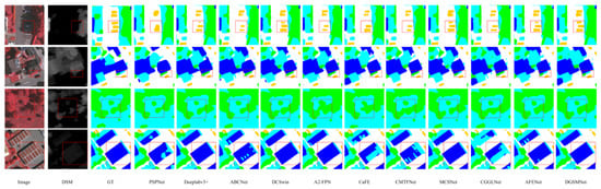
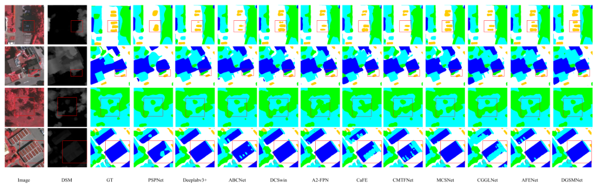
As shown in Figure 7, the first row presents the segmentation results of various networks for the few-shot vehicle category when vehicles are occluded by shadows and have colors similar to those of shadows. It can be seen that other methods fail to identify the vehicles in shadow areas or suffer from shape loss, while our network can recognize the vehicle contours well. The second row shows the segmentation performance when processing out-of-class similar objects. Other networks cannot distinguish the specific categories and tend to misclassify all targets as vegetation or trees. In contrast, DGSMNet fuses DSM information; it can be observed from the DSM that trees are obviously higher than vegetation, and the fusion of such information enables DGSMNet to distinguish trees from low vegetation more clearly. The third row demonstrates that DGSMNet can clearly distinguish categories and contour edges in scenarios with dense and interlaced vegetation and trees. The last row displays buildings with large intra-class differences; due to their color similarity to vegetation, some networks misclassify them as low vegetation, while DGSMNet can recognize the complete building contours by enhancing category guidance.

Figure 7. The locally enlarged results of DGSMNet on the Vaihingen dataset and the comparisons with other state-of-the-art networks.

Results on the Potsdam Dataset: Table 2 reports quantitative comparisons on the Potsdam dataset. Our DGSMNet attains the best results with an F1 score of 93.28%, mIoU of 87.64%, and OA of 92.10%. Compared with CaFE, which achieves 91.75% F1, 85.04% mIoU, and 90.31% OA, DGSMNet improves mean F1 by 1.53%, mIoU by 2.60%, and OA by 1.79%. Against CGGLNet, which achieves 93.02% F1, 87.19% mIoU, and 91.80% OA, DGSMNet yields gains of 0.26%, 0.45%, and 0.30% in mean F1, mIoU, and OA, respectively. DGSMNet also outperforms other methods, demonstrating consistent gains and validating the effectiveness of the proposed category-guidance strategy.

To separate the contribution of the network from test-time augmentation (TTA), Table 3 reports single-scale, single-pass results for the complete DGSMNet. TTA provides only modest gains, while the single-pass model retains comparable performance on both datasets.

Table 3. Single-pass and test-time-augmentation results for DGSMNet.

Dataset	Inference	mIoU (%)	F1 (%)	OA (%)
Vaihingen	Single-pass	85.18	91.82	93.60
	TTA	85.41	91.96	93.71
Potsdam	Single-pass	87.39	93.12	91.95
	TTA	87.64	93.28	92.10

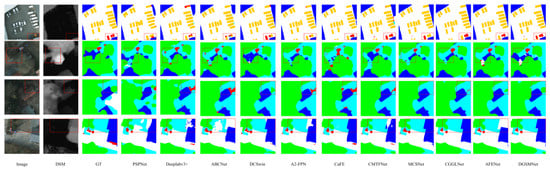
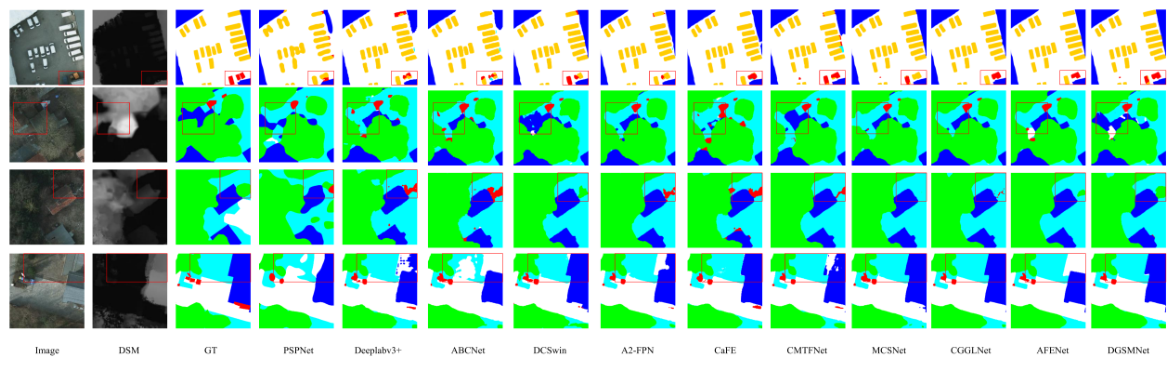
As shown in the first row of Figure 8, when dealing with extremely small objects with very low area proportions, most methods tend to misclassify them as cars with blurred boundaries. In contrast, DGSMNet, benefiting from its category enhancement mechanism, effectively recognizes such minority background objects and accurately delineates their contours. The second row illustrates buildings occluded by trees, where other methods commonly misclassify these regions as low vegetation and fail to recover clear boundaries due to tree interference. However, DGSMNet correctly identifies the building category and remains robust to occlusion effects. The third row presents scenarios with sparse tree canopies, in which existing methods either misclassify trees as background or produce incomplete segmentation, whereas DGSMNet achieves accurate and complete tree delineation. The last row demonstrates the boundary segmentation between large-scale low vegetation and buildings, where DGSMNet simultaneously distinguishes both categories while preserving precise and sharp boundary details.

Figure 8. The locally enlarged results of DGSMNet on the Potsdam dataset and the comparisons with other state-of-the-art networks.

5.2. Ablation Experiment

To verify the effectiveness of each component of the DGSMNet network, we conducted a series of ablation experiments on the Vaihingen and Potsdam datasets. In these experiments, we gradually removed individual modules and mainly focused on two evaluation metrics: mIoU and F1.

The cross-dataset ablation results are summarized in Table 4.

Table 4. Ablation experiments on the Vaihingen and Potsdam datasets.

Method	Vaihingen		Potsdam
	mIoU (%)	F1 (%)	mIoU (%)	F1 (%)
Baseline	82.72	90.31	84.46	91.55
Baseline + DSCG	84.54	91.43	86.42	92.38
Baseline + SPM	84.14	91.20	86.71	92.54
Baseline + DSCG + SPM	85.41	91.96	87.64	93.28

Table 5 further isolates the internal components of DSCG and SPM. Relative to the baseline, WGM alone improves mIoU by 1.23 percentage points, while adding FGM provides a further 0.59-point gain. The 2D-SSM and spatial branches improve mIoU by 1.03 and 0.78 points, respectively, and their combination reaches 84.14% mIoU. Under the same protocol, adding DSM to the RGB input improves mIoU, F1, and OA by 0.81, 0.49, and 0.20 percentage points, respectively. These results show that WGM and FGM provide complementary spatial and channel guidance, the two SPM branches contribute complementary long-range and directional spatial information, and DSM provides useful height cues.

Table 5. Component- and modality-level ablation on the Vaihingen dataset.

Module	Variant	mIoU (%)	F1 (%)	OA (%)
DSCG	Baseline	82.72	90.31	92.98
	WGM only	83.95	91.05	93.34
	WGM + FGM	84.54	91.43	93.47
SPM	Baseline	82.72	90.31	92.98
	2D-SSM only	83.75	90.91	93.28
	Spatial branch only	83.50	90.78	93.21
	2D-SSM + spatial branch	84.14	91.20	93.33
Input	RGB only	84.60	91.47	93.51
	RGB + DSM	85.41	91.96	93.71

Table 6 shows that the performance is stable around the selected loss weight. The best result is obtained at ${\lambda }_{\mathrm{wgm}}=0.4$, while weaker or stronger alignment supervision produces slightly lower scores.

Table 6. Sensitivity to the WGM loss weight on the Vaihingen dataset.

${\mathit{\lambda }}_{\mathbf{wgm}}$	mIoU (%)	F1 (%)	OA (%)
0.2	85.22	91.84	93.64
0.4	85.41	91.96	93.71
0.6	85.33	91.90	93.67
0.8	85.17	91.81	93.61

The incremental DSCG ablation results are reported in Table 7.

Table 7. Ablation study on the Vaihingen dataset with incremental addition of DSCG.

Guide Modules				F1 (%)					Evaluation Index
DSCG1	DSCG2	DSCG3	DSCG4	Imp.Surf.	Building.	Lowveg.	Tree	Car	mIoU (%)	F1 (%)	OA (%)
√				96.89	95.76	84.14	90.25	88.22	83.92	91.05	93.28
√	√			96.83	95.52	84.83	90.10	88.87	84.18	91.23	93.33
√	√	√		96.87	95.80	84.13	90.17	88.35	83.94	91.07	93.30
√	√	√	√	97.00	95.92	84.55	90.28	89.39	84.54	91.43	93.47

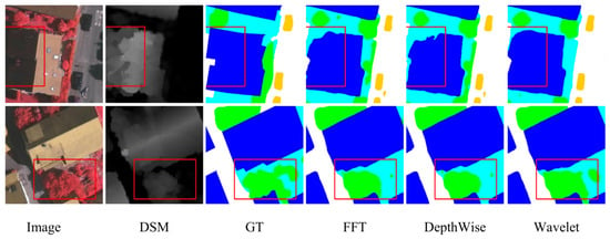
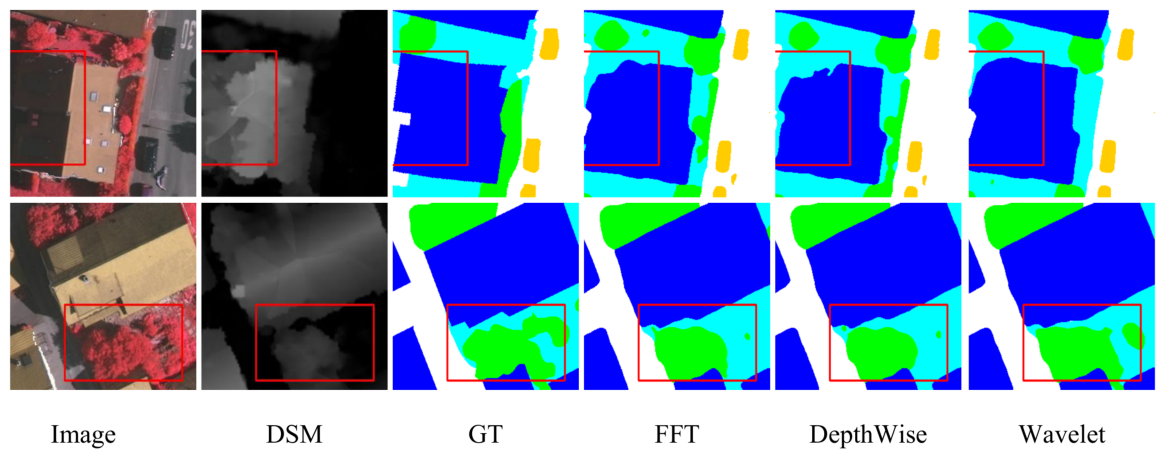
The comparison of feature extractors is reported in Table 8, and the corresponding qualitative results are shown in Figure 9.

Table 8. Comparison of different feature extractors on the Vaihingen dataset.

Methods	Params	Flops	mIoU (%)	F1 (%)	OA (%)
FFT	45.37	44.84	85.16	91.75	93.61
Depthwise	45.77	45.16	85.01	91.72	93.55
Wavelet (Ours)	48.85	51.56	85.41	91.96	93.71

Figure 9. Comparison of different feature extraction methods. The first row shows the segmentation results of building edges, and the second row presents the segmentation effects of different methods in the case of adjacent trees and vegetation.

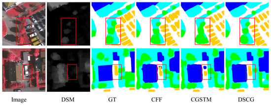
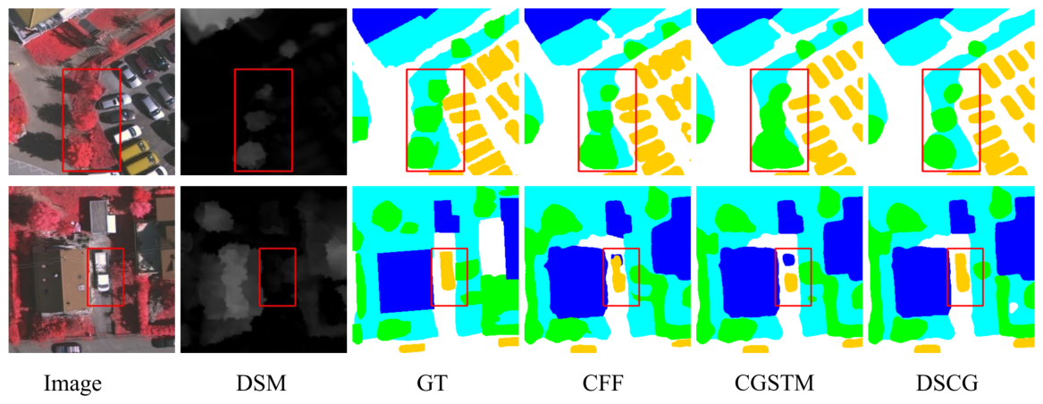
The comparison of category-guided modules is reported in Table 9, and the corresponding qualitative results are shown in Figure 10.

Table 9. Comparison of different category-guided modules on the Vaihingen dataset.

Modules	Params	Flops	mIoU (%)	F1 (%)	OA (%)
CFF [26]	52.42	50.26	84.62	91.53	93.42
CGSTM [18]	94.00	48.81	84.91	91.64	93.50
DSCG (Ours)	48.85	51.56	85.41	91.96	93.71

Figure 10. Segmentation results of different category-guided modules. The first row shows the segmentation results for few-shot trees, and the second row shows trucks that account for a small proportion of the car category.

(1) Components of DGSMNet: As presented in Table 4, each component in the proposed DGSMNet contributes progressively to enhancing segmentation performance. The complete DGSMNet achieves the highest scores, reaching 85.41% mIoU and 91.96% F1 on the Vaihingen dataset, and 87.64% mIoU and 93.28% F1 on the Potsdam dataset. The baseline model, which adopts a U-Net framework with ConvNeXt-Tiny as the backbone, attains 82.72% mIoU and 90.31% F1 on Vaihingen, and 84.46% mIoU and 91.55% F1 on Potsdam. Incorporating the DSCG improves mIoU by 1.82 and 1.96 percentage points and F1 by 1.12 and 0.83 points on the two datasets, respectively, demonstrating the contribution of category-specific spatial and channel guidance. The addition of the SPM improves mIoU by 1.42 and 2.25 points and F1 by 0.89 and 0.99 points, validating its contribution to spatial modeling. When both DSCG and SPM modules are integrated, DGSMNet achieves the best overall performance on both datasets, confirming the complementary effects of category guidance and spatial refinement.

The incremental SPM ablation results are reported in Table 10.

Table 10. Ablation study on the Vaihingen dataset with incremental addition of SPM.

Mamba Modules				F1 (%)					Evaluation Index
SPM1	SPM2	SPM3	SPM4	Imp.Surf.	Building.	Lowveg.	Tree	Car	mIoU (%)	F1 (%)	OA (%)
√				96.86	95.69	84.40	90.27	87.51	83.74	90.95	93.26
√	√			96.85	95.74	83.97	90.11	88.52	83.90	91.04	93.21
√	√	√		96.93	95.65	84.75	90.11	88.55	84.14	91.20	93.33
√	√	√	√	96.88	95.79	83.61	89.66	88.55	83.68	90.90	93.16

Note: The final DGSMNet contains SPM1–SPM3 at $H/4$, $H/8$, and $H/16$, respectively. SPM4 denotes an additional $H/32$ candidate stage evaluated only in this decoder-depth ablation and is not used in the final model.

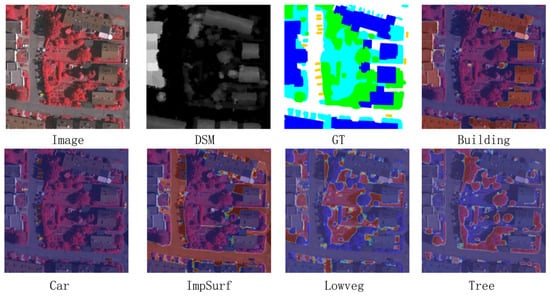
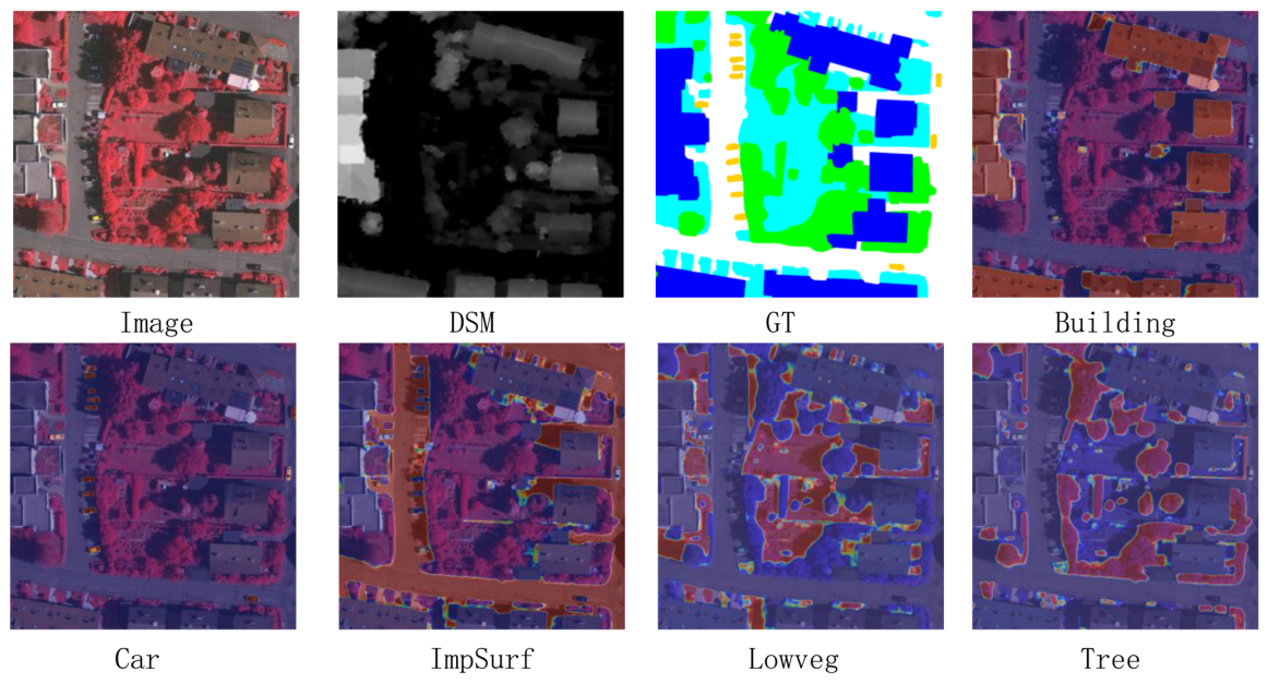
The feature heatmaps are shown in Figure 11.

Figure 11. Heatmaps of the final results, where the heatmap for the features of each corresponding category is separated and overlaid on the original image. The activated units in the heatmap correspond to the categories of the respective objects.

The patch-size comparison is reported in Table 11.

Table 11. Comparison of different patch sizes on the Vaihingen dataset.

Patch Size	mIoU (%)	F1 (%)	OA (%)
4	84.76	91.63	93.61
6	84.94	91.67	93.59
8	85.04	91.68	93.63
2 (ours)	85.41	91.96	93.71

The backbone comparison is reported in Table 12.

Table 12. Comparison of different backbone networks on the Vaihingen dataset.

Backbone	mIoU (%)	F1 (%)
ResNet18	84.81	91.61
ResNet50	84.54	91.44
ResNeXt50	84.94	91.69
ConvNeXt-Tiny	85.41	91.96

(2) Impact of DSCG: As shown in Table 7, progressively inserting the proposed DSCG modules into different stages leads to consistent performance gains. Even introducing DSCG at a single stage already brings clear improvements over the baseline, verifying the effectiveness of category-guided enhancement. When all four DSCG modules are integrated, the model achieves the best performance, reaching 84.54% mIoU and 91.43% F1 on the Vaihingen dataset.

To assess the feature extractor within DSCG, we replace the wavelet transform with FFT and depthwise convolution in Table 8. Wavelet extraction improves mIoU by 0.25 and 0.40 percentage points over FFT and depthwise convolution, respectively, with corresponding F1 gains of 0.21 and 0.24 points. Figure 9 further shows more complete building boundaries and clearer separation of adjacent tree and low-vegetation regions, consistent with combining low-frequency region support and spatially localized directional details.

Additionally, Table 9 compares the proposed DSCG with two representative category-guided modules, namely CFF and CGSTM. Despite using fewer parameters and similar FLOPs, DSCG achieves superior accuracy across all evaluation metrics. These results validate that DGSMNet provides more effective spatial semantic modulation than previous category-guided strategies. As shown in Figure 10, the first row presents the segmentation results for the tree category with a small proportion in the image. CFF and CGSTM fail to identify trees accurately and tend to misclassify vegetation as trees, while DSCG can achieve accurate recognition. The second row shows the recognition results for the car, a few-shot category; the truck carriage in the image is dissimilar to ordinary cars, so other methods are prone to misclassifying it as a building, whereas DSCG can recognize the complete vehicle after category-guided enhancement. In summary, DSCG yields consistent, cumulative improvements.

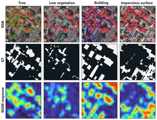
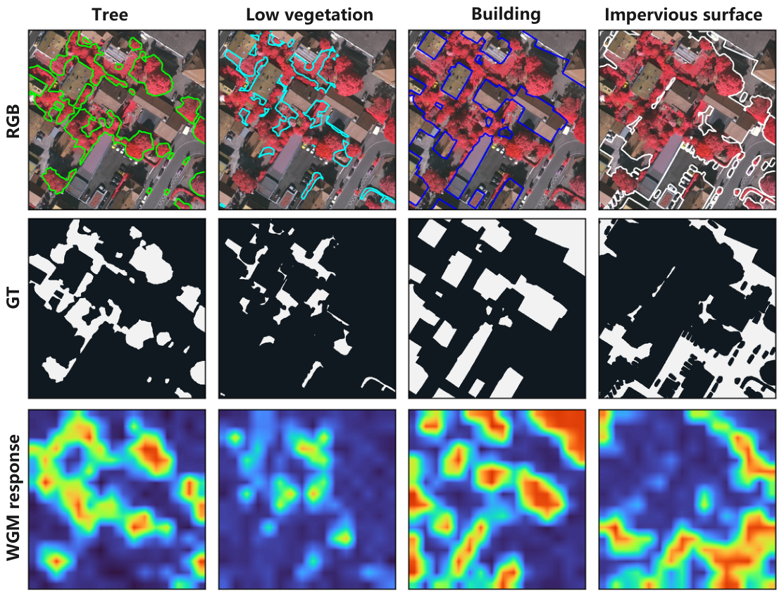
Figure 12 shows the class-specific WGM response maps from encoder Stage 4. The tree, low-vegetation, building, and impervious-surface channels exhibit high responses in their corresponding ground-truth regions. Owing to the coarser Stage 4 resolution, the response boundaries are smoother than those in the ground truth.

Figure 12. Visualization of class-specific WGM response maps from encoder Stage 4 on a Vaihingen test image. Rows show the RGB image with class contours, binary ground truth (GT), and WGM responses; columns correspond to tree, low vegetation, building, and impervious surface. The response maps are upsampled for visualization.The colors represent the activated units in the heatmap.

(3) Impact of the SPM: Table 11 shows that asymmetric small patches are most effective: our $1\times 2$ and $2\times 1$ settings achieve the best result, while larger patches, including 4, 6, and 8, yield marginally lower accuracy. We attribute this to $1\times 2$ and $2\times 1$ patches better capturing anisotropic, directional edge cues in aerial images.

Table 10 evaluates the decoder depth. SPM1–SPM3 correspond to the three decoder stages used in the final DGSMNet, whereas SPM4 is an additional candidate stage introduced only for this ablation. The three-stage configuration achieves the best performance, with 84.14% mIoU and 91.20% F1; adding the experimental fourth stage reduces the scores to 83.68% mIoU and 90.90% F1. The final architecture therefore retains three SPM modules, consistent with the network description in Section 3.2. Although adding SPM4 increases decoder depth and model capacity, it reduces mIoU from 84.14% to 83.68%, suggesting that the improvement of the selected three-stage design is not a simple consequence of increased network capacity. In terms of implementation, the key components are vertical and horizontal tokenization. After obtaining the SPM outputs, we further analyzed the corresponding heatmaps. Figure 11 shows that the model is able to focus on the discriminative structures of different categories, such as the geometric shapes of building roofs and the compact high-contrast regions of cars. These observations indicate that the network effectively integrates spatial and height information, enabling accurate localization of category-specific features and improving segmentation performance across multiple urban classes.

(4) Impact of Backbone: To assess the influence of different backbone networks on DGSMNet, we conducted experiments on the Vaihingen dataset using several widely adopted models, including ResNet18, ResNet50, ResNeXt50, and ConvNeXt-Tiny. As shown in Table 12, ConvNeXt-Tiny achieves the best performance with 85.41% mIoU and 91.96% F1, outperforming other backbones. Although ResNet-based models deliver competitive results, ConvNeXt-Tiny demonstrates stronger feature representation and better compatibility with the re-encoder structure of DGSMNet. Therefore, ConvNeXt-Tiny is selected as the backbone for subsequent experiments, providing an effective balance between accuracy and efficiency.

5.3. Model Parameters and Computational Complexity Analysis

Table 13 compares parameter counts and FLOPs for several competing networks.

Table 13. Comparison of parameters and computation of different networks.

Method	Params (M)	FLOPs (G)
PSPNet [10]	53.3	28.1
DeeplabV3+ [32]	40.3	138.6
ABCNet [33]	13.6	15.7
DC-Swin [34]	66.9	72.1
$A^2$-FPN [35]	22.8	41.7
CaFE [26]	52.42	50.26
CMTFNet [36]	30.1	34.3
MCSNet [37]	54.7	63.9
CGGLNet [18]	34.83	48.81
AFENet [38]	20.23	25.59
DGSMNet (ours)	63.9	74.4

DGSMNet uses 63.9M parameters and 74.4G FLOPs, which are larger than those of most baselines, but it yields superior segmentation performance. This indicates a trade-off where increased model capacity and computation lead to improved accuracy.

6. Discussion

6.1. Effect of Category Guidance

The results across the Vaihingen and Potsdam datasets indicate that category guidance can reduce the adverse effects of class imbalance under the evaluated protocols. The DSCG module improves the representation of minority classes by providing class-aware spatial and channel guidance before the final prediction stage. On Vaihingen, the car F1 gain over CGGLNet is 2.66 points, while using DSCG at all four encoder stages raises car F1 from 88.22% with one guided stage to 89.39%. The ablation results further suggest that the WGM and FGM components are complementary: WGM provides spatially localized class priors, whereas FGM expands these priors into the channel dimension for feature reweighting.

6.2. Effect of Spatial Modeling and Computational Cost

The SPM module improves the modeling of long-range spatial dependencies while preserving local details through horizontal and vertical feature sequences. The qualitative results show that this design is particularly useful for small objects, occluded regions, and boundaries between visually similar classes. The parameter and FLOP comparison also reveals a trade-off: DGSMNet achieves higher segmentation accuracy at the cost of a larger model and greater computational demand than several baseline networks. The current ablations do not include a parameter- or FLOP-matched replacement of SPM with a conventional convolutional or attention-based decoder block. Consequently, they do not fully separate the architectural benefit of SPM from differences in capacity and computational cost; such a controlled comparison remains for future work.

6.3. Limitations and Future Work

This study evaluates the proposed method on the Vaihingen and Potsdam benchmarks, and its generalization to other sensors, geographic regions, resolutions, and class taxonomies remains to be established. The current experiments also focus on a single primary backbone and do not provide a cross-dataset transfer evaluation. Future work will investigate broader cross-domain validation, more efficient model variants, and public release of the training and evaluation pipeline to facilitate reproducibility.

7. Conclusions

This paper proposes DGSMNet, a category-guided remote sensing semantic segmentation network. It employs DSCG to help the network acquire category information and integrates spatial information into the network through decoding via SPM. In DSCG, the WGM module first extracts high- and low-frequency information from objects, which is then converted into feature attention maps corresponding to category features. Based on the attention maps generated by WGM, the FGM module expands them and multiplies them with input features, ensuring the channel proportion of different features during model learning. Finally, the SPM establishes long-range modeling while integrating spatial information into the network, enabling the model to better understand spatial information in images. Experiments on Vaihingen and Potsdam show competitive performance and support the contribution of the proposed components under the evaluated settings. Generalization to other geographic regions, sensors, resolutions, and class taxonomies remains to be established.

References

- Zao, Y.; Zou, Z.; Shi, Z. Topology-Guided Road Graph Extraction From Remote Sensing Images. IEEE Trans. Geosci. Remote Sens. 2024, 62, 1–14. [Google Scholar] [CrossRef] [Scilit]
- Yokoya, N.; Yamanoi, K.; He, W.; Baier, G.; Adriano, B.; Miura, H.; Oishi, S. Breaking Limits of Remote Sensing by Deep Learning From Simulated Data for Flood and Debris-Flow Mapping. IEEE Trans. Geosci. Remote Sens. 2022, 60, 1–15. [Google Scholar] [CrossRef] [Scilit]
- Mountrakis, G.; Heydari, S.S. Harvesting the Landsat Archive for Land Cover Land Use Classification Using Deep Neural Networks: Comparison with Traditional Classifiers and Multi-Sensor Benefits. ISPRS J. Photogramm. Remote Sens. 2023, 200, 106–119. [Google Scholar] [CrossRef] [Scilit]
- Li, Z.; Chen, B.; Wu, S.; Su, M.; Chen, J.M.; Xu, B. Deep Learning for Urban Land Use Category Classification: A Review and Experimental Assessment. Remote Sens. Environ. 2024, 311, 114290. [Google Scholar] [CrossRef] [Scilit]
- Mountrakis, G.; Im, J.; Ogole, C. Support Vector Machines in Remote Sensing: A Review. ISPRS J. Photogramm. Remote Sens. 2011, 66, 247–259. [Google Scholar] [CrossRef] [Scilit]
- Zhu, X.X.; Tuia, D.; Mou, L.; Xia, G.S.; Zhang, L.; Xu, F.; Fraundorfer, F. Deep Learning in Remote Sensing: A Comprehensive Review and List of Resources. IEEE Geosci. Remote Sens. Mag. 2017, 5, 8–36. [Google Scholar] [CrossRef] [Scilit]
- Long, J.; Shelhamer, E.; Darrell, T. Fully Convolutional Networks for Semantic Segmentation. In Proceedings of the 2015 IEEE Conference on Computer Vision and Pattern Recognition (CVPR), Boston, MA, USA, 7–12 June 2015; pp. 3431–3440. [Google Scholar]
- Badrinarayanan, V.; Kendall, A.; Cipolla, R. Segnet: A deep convolutional encoder-decoder architecture for image segmentation. IEEE Trans. Pattern Anal. Mach. Intell. 2017, 39, 2481–2495. [Google Scholar] [CrossRef] [Scilit]
- Ronneberger, O.; Fischer, P.; Brox, T. U-Net: Convolutional Networks for Biomedical Image Segmentation. In Proceedings of the Medical Image Computing and Computer-Assisted Intervention—MICCAI 2015; Navab, N., Hornegger, J., Wells, W.M., Frangi, A.F., Eds.; Springer: Cham, Switzerland, 2015; pp. 234–241. [Google Scholar]
- Zhao, H.; Shi, J.; Qi, X.; Wang, X.; Jia, J. Pyramid Scene Parsing Network. In Proceedings of the IEEE Conference on Computer Vision and Pattern Recognition (CVPR), Honolulu, HI, USA, 22–25 July 2017; pp. 6230–6239. [Google Scholar]
- Chen, L.C.; Papandreou, G.; Kokkinos, I.; Murphy, K.; Yuille, A.L. Semantic image segmentation with deep convolutional nets and fully connected CRFs. arXiv 2014, arXiv:1412.7062. [Google Scholar]
- Chen, L.C.; Papandreou, G.; Kokkinos, I.; Murphy, K.; Yuille, A.L. Deeplab: Semantic image segmentation with deep convolutional nets, atrous convolution, and fully connected crfs. IEEE Trans. Pattern Anal. Mach. Intell. 2017, 40, 834–848. [Google Scholar] [CrossRef] [Scilit]
- Chen, L.C.; Papandreou, G.; Schroff, F.; Adam, H. Rethinking atrous convolution for semantic image segmentation. arXiv 2017, arXiv:1706.05587. [Google Scholar]
- Cui, J.; Liu, J.; Ni, Y.; Wang, J.; Li, M. FDGSNet: A Multimodal Gated Segmentation Network for Remote Sensing Image Based on Frequency Decomposition. IEEE J. Sel. Top. Appl. Earth Obs. Remote Sens. 2024, 17, 19756–19770. [Google Scholar] [CrossRef] [Scilit]
- Ma, X.; Zhang, X.; Pun, M.O.; Liu, M. A Multilevel Multimodal Fusion Transformer for Remote Sensing Semantic Segmentation. IEEE Trans. Geosci. Remote Sens. 2024, 62, 1–15. [Google Scholar] [CrossRef] [Scilit]
- Jing, W.; Zhang, W.; Di, D.; Li, C.; Emam, M.; Mian, A. Hypergraph BiFormer for Semantic Segmentation of High-Resolution Remote Sensing Images. IEEE Trans. Geosci. Remote Sens. 2025, 63, 1–15. [Google Scholar] [CrossRef] [Scilit]
- Ma, X.; Ma, M.; Hu, C.; Song, Z.; Zhao, Z.; Feng, T.; Zhang, W. Log-Can: Local-Global Class-Aware Network for Semantic Segmentation of Remote Sensing Images. In Proceedings of the ICASSP 2023—2023 IEEE International Conference on Acoustics, Speech and Signal Processing (ICASSP), Rhodes Island, Greece, 4–10 June 2023; pp. 1–5. [Google Scholar]
- Ni, Y.; Liu, J.; Chi, W.; Wang, X.; Li, D. CGGLNet: Semantic Segmentation Network for Remote Sensing Images Based on Category-Guided Global–Local Feature Interaction. IEEE Trans. Geosci. Remote Sens. 2024, 62, 1–17. [Google Scholar] [CrossRef] [Scilit]
- Zeng, J.; Gu, Y.; Qin, C.; Jia, X.; Deng, S.; Xu, J.; Tian, H. Unsupervised Domain Adaptation for Remote Sensing Semantic Segmentation with the 2D Discrete Wavelet Transform. Sci. Rep. 2024, 14, 23552. [Google Scholar] [CrossRef] [Scilit]
- Li, Y.; Liu, Z.; Yang, J.; Zhang, H. Wavelet Transform Feature Enhancement for Semantic Segmentation of Remote Sensing Images. Remote Sens. 2023, 15, 5644. [Google Scholar] [CrossRef] [Scilit]
- Wang, L.; Li, R.; Zhang, C.; Fang, S.; Duan, C.; Meng, X.; Atkinson, P.M. UNetFormer: A UNet-like transformer for efficient semantic segmentation of remote sensing urban scene imagery. ISPRS J. Photogramm. Remote Sens. 2022, 190, 196–214. [Google Scholar] [CrossRef] [Scilit]
- Ma, X.; Wu, Q.; Zhao, X.; Zhang, X.; Pun, M.O.; Huang, B. SAM-Assisted Remote Sensing Imagery Semantic Segmentation with Object and Boundary Constraints. IEEE Trans. Geosci. Remote Sens. 2024, 62, 1–16. [Google Scholar] [CrossRef] [Scilit]
- Li, X.; Xu, F.; Yu, A.; Lyu, X.; Gao, H.; Zhou, J. A Frequency Decoupling Network for Semantic Segmentation of Remote Sensing Images. IEEE Trans. Geosci. Remote Sens. 2025, 63, 1–21. [Google Scholar] [CrossRef] [Scilit]
- Wang, T.; Chen, G.; Zhang, X.; Liu, C.; Wang, J.; Tan, X.; Zhou, W.; He, C. LMFNet: Lightweight Multimodal Fusion Network for high-resolution remote sensing image segmentation. Pattern Recognit. 2025, 164, 111579. [Google Scholar] [CrossRef] [Scilit]
- Liu, Y.; Gao, K.; Wang, H.; Yang, Z.; Wang, P.; Ji, S.; Huang, Y.; Zhu, Z.; Zhao, X. A Transformer-based multi-modal fusion network for semantic segmentation of high-resolution remote sensing imagery. Int. J. Appl. Earth Obs. Geoinf. 2024, 133, 104083. [Google Scholar] [CrossRef] [Scilit]
- Zheng, A.; He, J.; Wang, M.; Li, C.; Luo, B. Category-Wise Fusion and Enhancement Learning for Multimodal Remote Sensing Image Semantic Segmentation. IEEE Trans. Geosci. Remote Sens. 2022, 60, 1–12. [Google Scholar] [CrossRef] [Scilit]
- Ma, X.; Che, R.; Hong, T.; Ma, M.; Zhao, Z.S.; Feng, T.; Zhang, W. SACANet: Scene-aware class attention network for semantic segmentation of remote sensing images. In Proceedings of the 2023 IEEE International Conference on Multimedia and Expo (ICME), Brisbane, Australia, 10–14 July 2023; pp. 828–833. [Google Scholar]
- He, X.; Zhou, Y.; Liu, B.; Zhao, J.; Yao, R. Remote sensing image semantic segmentation via class-guided structural interaction and boundary perception. Expert Syst. Appl. 2024, 252, 124019. [Google Scholar] [CrossRef] [Scilit]
- Liu, Y.; Tian, Y.; Zhao, Y.; Yu, H.; Xie, L.; Wang, Y.; Ye, Q.; Jiao, J.; Liu, Y. VMamba: Visual State Space Model. In Proceedings of the Advances in Neural Information Processing Systems; Globerson, A., Mackey, L., Belgrave, D., Fan, A., Paquet, U., Tomczak, J., Zhang, C., Eds.; Curran Associates, Inc.: Red Hook, NY, USA, 2024; Volume 37, pp. 103031–103063. [Google Scholar]
- Ma, X.; Zhang, X.; Pun, M.O. RS3Mamba: Visual State Space Model for Remote Sensing Image Semantic Segmentation. IEEE Geosci. Remote Sens. Lett. 2024, 21, 1–5. [Google Scholar] [CrossRef] [Scilit]
- Gao, L.; Li, X.; Liu, Y.; Chen, X.; Liu, Y.; Xu, J.; Zhang, M. SkyMamba: Integrating Transformer and State-Space Model for UAV Remote Sensing RGB-D Images Semantic Segmentation. IEEE Trans. Geosci. Remote Sens. 2025, 63, 1–18. [Google Scholar] [CrossRef] [Scilit]
- Chen, L.C.; Zhu, Y.; Papandreou, G.; Schroff, F.; Adam, H. Encoder-Decoder with Atrous Separable Convolution for Semantic Image Segmentation. In Proceedings of the Computer Vision—ECCV 2018; Springer: Cham, Switzerland, 2018; Volume 11211, pp. 833–851. [Google Scholar]
- Li, R.; Zheng, S.; Zhang, C.; Duan, C.; Wang, L.; Atkinson, P.M. ABCNet: Attentive bilateral contextual network for efficient semantic segmentation of Fine-Resolution remotely sensed imagery. ISPRS J. Photogramm. Remote Sens. 2021, 181, 84–98. [Google Scholar] [CrossRef] [Scilit]
- Wang, L.; Li, R.; Duan, C.; Zhang, C.; Meng, X.; Fang, S. A novel transformer based semantic segmentation scheme for fine-resolution remote sensing images. IEEE Geosci. Remote Sens. Lett. 2022, 19, 1–5. [Google Scholar] [CrossRef] [Scilit]
- Li, R.; Wang, L.; Zhang, C.; Duan, C.; Zheng, S. A2-FPN for semantic segmentation of fine-resolution remotely sensed images. Int. J. Remote Sens. 2022, 43, 1131–1155. [Google Scholar] [CrossRef] [Scilit]
- Wu, H.; Huang, P.; Zhang, M.; Tang, W.; Yu, X. CMTFNet: CNN and Multiscale Transformer Fusion Network for Remote-Sensing Image Semantic Segmentation. IEEE Trans. Geosci. Remote Sens. 2023, 61, 1–12. [Google Scholar] [CrossRef] [Scilit]
- Chen, Y.; Wang, Y.; Xiong, S.; Lu, X.; Zhu, X.X.; Mou, L. Integrating detailed features and global contexts for semantic segmentation in ultra-high-resolution remote sensing images. IEEE Trans. Geosci. Remote Sens. 2024, 62, 1–14. [Google Scholar] [CrossRef] [Scilit]
- Gao, F.; Fu, M.; Cao, J.; Dong, J.; Du, Q. Adaptive Frequency Enhancement Network for Remote Sensing Image Semantic Segmentation. IEEE Trans. Geosci. Remote Sens. 2025, 63, 1–15. [Google Scholar] [CrossRef] [Scilit]
Disclaimer/Publisher’s Note: The statements, opinions and data contained in all publications are solely those of the individual author(s) and contributor(s) and not of MDPI and/or the editor(s). MDPI and/or the editor(s) disclaim responsibility for any injury to people or property resulting from any ideas, methods, instructions or products referred to in the content. |
© 2026 by the authors. Licensee MDPI, Basel, Switzerland. This article is an open access article distributed under the terms and conditions of the Creative Commons Attribution (CC BY) license.