An Explainable Machine Learning Framework for Sentinel-1 SAR Wave-Mode Significant Wave Height Retrieval via Spotter-Buoy-Corrected ERA5 Reanalysis

Highlights

What are the main findings?

• Quantile-mapping correction using Spotter buoys effectively removes sea-state-dependent biases in ERA5 SWH, improving the SAR retrieval dynamic range.
• XGBoost model achieves RMSEs of 0.36 m (WV1) and 0.45 m (WV2) against independent drifting Spotter buoy data across 0.5–10.0 m SWH.

What are the implications of the main findings?

• SHAP analysis identifies λ_c and cvar as dominant predictors, providing physical interpretability for SAR-based SWH retrieval.
• A compact 12-feature model retains near-equivalent performance, enabling efficient and transparent SWH monitoring from Sentinel-1.

Abstract

Significant wave height (SWH) is a fundamental parameter for ocean engineering, maritime safety, and climate studies. Although spaceborne synthetic aperture radar (SAR) wave mode observations provide global, all-weather coverage, accurate SWH retrieval remains challenging due to the complex ocean-to-SAR imaging mechanism. This paper presents an explainable machine learning algorithm for retrieving SWH from Sentinel-1 SAR wave mode data. To address the scarcity of high-quality collocations and the black-box nature of existing deep-learning approaches, we first correct ERA5 SWH against high-quality Spotter drifting in situ using quantile mapping (QM). The bias-corrected ERA5 data are then collocated with Sentinel-1 SAR to generate a large-scale, globally distributed, and Spotter-calibrated training dataset. Here, QM maps each quantile of the ERA5 data distribution onto the corresponding quantile of the collocated Spotter distribution, thereby adjusting the statistical distribution of the reanalysis. An eXtreme gradient boosting regression model is then trained on 32 physically interpretable features extracted from Sentinel-1 Level-2 products, including image statistics, spectral parameters, azimuth cutoff wavelength, normalized radar cross section, and wind-related variables. Comprehensive temporal-independent validations against Spotter buoys and multi-mission altimeter data throughout one year of 2021 (excluded both from the QM correction and from model training) demonstrate high accuracy, with root-mean-square errors of 0.36 m (WV1) and 0.45 (WV2) for SAR–Spotter matchups over the range 0.5–10.0 m. In addition, SHapley Additive exPlanation (SHAP) analysis is employed to quantify feature contributions and enhance model transparency. Furthermore, a compact 12-feature model selected via SHAP-based hierarchical clustering retains a nearly equivalent performance while improving interpretability. The proposed approach offers a reliable and transparent solution for global SAR-based SWH monitoring.

1. Introduction

Sea state is fundamental to oceanography for understanding momentum and heat exchange at the air–sea interface and the broader global climate system. Ocean wave measurements are also essential for ocean engineering, maritime situational awareness, and the protection of coastal infrastructure against extreme events. Significant wave height (SWH), defined as the average height of the highest one-third of waves, is the most widely utilized bulk parameter for wave monitoring. Nowadays, remotely sensed data serve as an indispensable data source for sea state monitoring while traditional in situ buoy networks are severely limited. For instance, SWH monitored by satellites is part of the ECVs (Essential Climate Variables) in the European Space Agency’s (ESA) Climate Change Initiative (CCI) program.

Spaceborne synthetic aperture radars (SARs), particularly those operating in wave mode, have proven highly successful in observing the SWH at a global scale independent of solar illumination and largely unaffected by cloud cover. For decades, C-band SAR wave mode acquisitions from European ERS-1/2 [1], Envisat ASAR [2,3], Sentinel-1 series [4] and Chinese Gaofen-3 mission have contributed to long-term SAR-derived SWH archive.

However, inverting SWH from SAR images is not straightforward due to the complex and nonlinear ocean-to-SAR imaging mechanism [5]. To date, SWH retrieval from SAR is generally divided into three main categories: theoretical (physics-based), empirical (conventional statistics-based), and machine learning algorithms.

Theoretical approaches aim to first invert the SAR image spectrum into an ocean wave spectrum based on the complex SAR wave mapping forward transform, then compute SWH via 2D spectral integration. Milestone algorithms include the Max-Planck Institute (MPI) scheme [6,7], Semi-Parametric Retrieval Algorithm (SPRA) [8], Partition Rescaling and Shift Algorithm (PARSA) [9], and parameterized first-guess spectrum method (PFSM) [10]. These theoretical methods can provide detailed spectral information. However, they are computationally expensive due to the iterative inversion process and require prior wind information to generate a first-guess wave spectrum. Moreover, they tend to perform poorly under extreme sea states, where nonlinear distortions and the azimuthal cutoff effect often bring significant information loss.

These difficulties spurred the development of data-driven alternatives. In contrast to theoretical schemes, empirical models establish a direct relationship between SAR image features and SWH, thereby avoiding the sophisticated intermediate step of the full wave spectrum retrieval. A representative empirical approach is the CWAVE model family, which was originally developed for ERS-2 by Schulz-Stellenfleth et al. [4], and later adapted for other C-band SAR wave mode data, (e.g., Envisat (CWAVE_ENV) [11], Sentinel-1A (CWAVE_S1A) [12] and Gaofen-3 (QPCWAVE_GF3) [13]). The CWAVE empirical framework has also been extended to the XWAVE model for X-band SAR missions [14,15]. These empirical functions are convenient and robust, making them suitable for near-real-time (NRT) services [16,17]. Nevertheless, the complicated relationships between SAR data and SWH are often inadequately represented by the conventional statistical regression (e.g., second-order polynomial).

In the era of big data, Artificial Intelligence (AI) technologies have gained considerable attention in satellite oceanography [18]. In particular, machine- and deep-learning models for inferring SWH from SAR imagery have emerged in recent years. These efforts include deep neural networks [4,19,20], convolutional neural networks (CNNs) [21,22], deep residual networks [23,24] and eXtreme Gradient Boosting (XGBoost) models [25] for estimating SWH from SAR data. These models can effectively learn the intricate patterns hidden within SAR SWH matchups, thereby significantly improving the SWH retrieval accuracy.

However, challenges remain regarding machine-learning-based SWH retrieval from SAR observations. A major limitation is the scarcity of high-quality labels for model training. Some researchers relied on the in situ SWH from sparsely distributed moored buoys, yielding a small training dataset and hindering comprehensive validation at a global scale. Others exploited the global wave models as the target, such as WaveWatchIII or ERA5 reanalysis from the European Centre for Medium-Range Weather Forecasts (ECMWF). These reanalysis datasets provide globally complete and temporally continuous SWH fields. Nevertheless, they are not error-free and contain sea-state-dependent biases. Another shortcoming of many machine- or deep-learning-based retrieval models is their black-box nature, which makes it difficult to diagnose the physical relevance of the learned SAR features and to assess model robustness.

In this paper, we aim to address the aforementioned challenges. Our main contributions are as follows:

(1)

A distribution-adjusted reanalysis labeling strategy. Spotter drifting buoys [26] provide high-quality in situ SWH measurements across broader open-ocean regions compared with conventional moored buoy networks, e.g., National Data Buoy Center [27] and the Coastal Data Information Program [28]. In this study, we derive sea-state-dependent bias corrections from Spotter observations and apply them to the original ERA5 SWHs. This strategy combines the global coverage and dynamical consistency of reanalysis with the accuracy advantages of in situ observations. By doing this, we curate and leverage Spotter-buoy-corrected ERA5 data to construct a larger, calibrated, and globally distributed training dataset.

(2)

Retrieval model and its accuracy assessment. We develop an XGBoost-based SWH retrieval model using physically meaningful SAR image and spectral features. The model is trained on the large-scale corrected reanalysis labels and extensively validated against independent Spotter buoys and altimeter-derived SWH. Here, we note that the choice of XGBoost is motivated by its suitability to tabular features and its native handling of nonlinearity and feature interaction. The added value here is validating against temporally independent Spotter and multi-mission altimeter observations.

(3)

Interpretability and model compression. We employ SHAP (SHapley Additive exPlanation) analysis but as a diagnostic tool to quantify feature contributions, thereby providing feature interpretability insights into the SAR SWH relationship and improving the transparency of data-driven SAR SWH retrieval models.

The remainder of this paper is organized as follows. The dataset is described in Section 2. Section 3 presents the method for construction of the Spotter-buoy-corrected ERA5 SWH and the XGBoost-based SAR SWH retrieval model. The performance against independent Spotter drifters and altimeters is given in Section 4. Discussion is provided in Section 5. Finally, concluding remarks are given in Section 6.

2. Datasets

2.1. Sentinel-1A/B Wave Mode Data

The Sentinel-1 mission is part of the ESA’s Copernicus Program and was designed as a constellation of C-band SAR satellites, including Sentinel-1A/B and the follow-on Sentinel-1C/D. The SAR sensors onboard Sentinel-1 operate in four imaging modes: interferometric wide swath, extra-wide swath, strip-map, and wave mode (WV). Among them, WV is specifically designed for open-ocean wave monitoring. In WV mode, Sentinel-1 collects consecutive 20 × 20 km SAR imagettes in VV polarization, sampling at two alternating incidence beams approximately 200 km apart. The acquisitions alternate between two incidence angles of approximately 23° and 36°, referred to as WV1 and WV2, respectively.

This study focused on Sentinel-1A/B Level-2 Ocean (OCN) products acquired in WV mode from Jan. 2021 to Mar. 2023. It should be noted that Sentinel-1B data are only available during the early part of the study period because of its sudden failure occurring in late 2021. Several quality controls were applied. First, filtering was carried out according to the normalized variance (cvar) of the SAR imagette intensity, with thresholds of 1.0–2.0 for WV1 and 1.0–1.4 for WV2, following Stopa and Mouche [4]. These thresholds were used to remove inhomogeneous imagettes affected by non-wave signatures. In addition, observations located poleward of 65° latitude were rejected to reduce the potential influence of sea ice contamination.

The Sentinel-1 Level-2 OCN products provide a set of geophysical and spectral parameters relevant to ocean wave retrieval, including normalized radar cross section (NRCS), cross spectra, and other SAR-derived wave parameters. These variables form the basis for the feature construction used in the proposed SAR-based SWH retrieval framework. The selected Sentinel-1 WV parameters used in this study are detailed in Section 3.3.

2.2. ECMWF ERA5 Reanalysis

ERA5 is the ECMWF’s fifth-generation global reanalysis providing hourly estimates of ocean wave parameters. Here, the ERA5 total significant wave height of combined wind waves and swell was used. The ERA5 wave fields are generated by the ECMWF Integrated Forecasting System coupled with the WAM wave model [29] and are offered on a 0.5° × 0.5° grid.

Here, only ERA5 grid points located more than 200 km offshore were used. This criterion was applied to reduce uncertainties related to unresolved coastal processes, complex bathymetry, wave refraction and diffraction, and possible land contamination in SAR imagettes.

Owing to its global spatial coverage and hourly temporal resolution, ERA5 provides a spatially and temporally continuous description of the sea state and has therefore been widely used as references when constructing SAR SWH training matchups and validation (e.g., [24,30,31,32]). Nevertheless, it may contain systematic sea-state-dependent errors. For instance, Wang et al. [33] reported that ERA5 tends to overestimate low sea states and underestimate high sea states. Therefore, directly using ERA5 as training labels may introduce bias into machine-learning retrieval models. To mitigate this issue, this study further corrects ERA5 SWH using Spotter-drifting-buoy observations, as described in Section 3.2.

2.3. Spoter Buoy Observations

In situ wave observations from Sofar Ocean Spotter drifting buoys were used in this study as the ground truth. The Spotter buoy is a compact, solar-powered directional wave measurement platform that estimates three-dimensional sea-surface displacement using GNSS and inertial sensors [26]. As a surface-following Lagrangian platform, Spotter hourly records wave-induced buoy motions, from which wave parameters are derived through spectral analysis of the displacement time series. The Spotter SWH records are estimated from the zeroth-order spectral moment. Previous studies have demonstrated that Spotter SWH measurements are in good agreement with conventional wave buoys, such as Waverider [34,35], and have been used for the calibration and validation of satellite ocean wave retrievals recently [36,37].

2.4. Altimeter Data

Altimeter SWH used in this study are obtained from the ESA CCI Sea State dataset. This dataset provides long-term SWH observations derived from the multi-mission of radar altimeters. All measurements are quality controlled and validated against in situ reference data, ensuring consistency among each other [38].

For the independent validation in this study, focus is placed on Jason-3, SARAL and Sentinel-6 SWH data for the year 2021, which have an approximate spatial resolution of 6 km along the tracks. Note that altimeter observations near land were excluded (less than 200 km offshore) in this study, since altimeter-derived SWH could be less accurate near the coast (e.g., [39]).

3. Methodology

3.1. Collocations

Three collocated datasets were constructed for ERA5 correction, XGBoost training, and independent validation, respectively.

(1)

ERA5 SWH was collocated with Spotter observations to establish the bias correction between the reanalysis and in situ SWH. For each Spotter record, the nearest ERA5 SWH in time and space was selected. The resulting Spotter–ERA5 matchup dataset was used to derive and evaluate the quantile-mapping correction (see Section 3.2). Specifically, the correction was constructed from 1,162,283 collocated Spotter–ERA5 pairs in 2022. And these matchups are distributed globally over the open ocean, which justifies applying one sea-state-dependent correction to the ERA5 SWH fields.

(2)

Sentinel-1 WV data were collocated with Spotter-corrected ERA5 SWH to construct the training dataset for the SAR SWH retrieval model. A temporal window of 0.5 h and a spatial threshold of 0.25° were used for collocation covering the period from April 2022 to March 2023. During this period, only Sentinel-1A data were used since Sentinel-1B data were unavailable. Large-scale matchups with an amount of 259,360 were obtained. The SAR–ERA5 matchups are randomly shuffled and split into groups on a Sentinel-1 satellite cycle basis: training set (75%) and internal testing set (25%) for hyperparameter searching set, respectively. This strategy was adopted to avoid temporal leakage.

(3)

Independent validation datasets were constructed by collocating Sentinel-1A/B WV data with external observation-based SWH references, including Spotter/altimeter-derived SWH dataset. For these validation datasets, a temporal window of 1 h and a spatial threshold of 100 km were adopted. Over the entire one year of 2021, 38,549 (63,069) SAR–Spotter (SAR–altimeter) matchups were obtained. Since this validation period is temporally separated from both Jan.-Mar. 2022 (Spotter used for ERA5 bias correction) and April 2022–March 2023 (Sentinel-1 used for XGBoost model training), these matchups provide an independent assessment of the generalization of our proposed retrieval model.

The 0.25°/0.5 h window used for SAR–ERA5 training matchups is set by the native resolution of the label field (ERA5 grid) rather than by the sparsity of in situ data. In contrast, independent validation against Spotter buoys and along-track altimeters requires a different compromise. A 100 km/1 h window follows common practice for Sentinel-1 WV Cal/Val (e.g., [4,19]) and is intended to retain enough globally distributed samples.

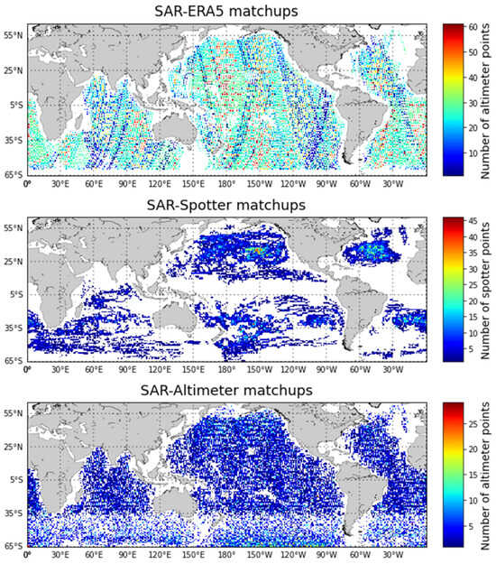
Figure 1 presents the geographical distribution of these matchup datasets. Figure 1 shows that the SAR–Spotter matchups are concentrated in the central and eastern Pacific and are relatively sparser in the other basins. The quantile-mapping correction (see below) used here is a single quantile mapping from ERA5 to Spotter SWH, so this imbalance does not enter as an explicit spatial predictor. Note that it can still affect global applicability if ERA5 errors vary among basins that are weakly sampled by Spotter.

Figure 1. Global distributions of SAR–ERA5, SAR–Spotter and SAR–altimeter collocations.

3.2. Calibration of ERA5 Significant Wave Height

Although ERA5 provides globally continuous SWH reanalysis, it may contain systematic sea-state-dependent biases. Directly using raw ERA5 as training labels may therefore propagate these biases into the SAR retrieval model. To mitigate this shortcoming, Spotter buoy observations were used as reference data to correct ERA5 SWH before training the XGBoost retrieval model. In this section, the quantile mapping (QM) correction method is introduced, a linear regression (LR) correction is implemented as a baseline, and its performance is evaluated.

(1)

Quantile-Mapping correction

To reduce the systematic sea-state-dependent bias in ERA5 SWH, a quantile mapping approach was applied using collocated Spotter buoy observations as the reference. The Spotter–ERA5 collocation dataset was used to establish the statistical relationship between ERA5 SWH and in situ buoy-measured SWH.

Quantile mapping is a distribution-based bias-correction method that adjusts the statistical distribution of model or reanalysis data to match that of reference observations [40,41,42]. Compared with a simple mean-bias correction, QM can account for sea-state-dependent errors by correcting different parts of the SWH distribution separately. Let $H_s^E$ and $H_s^S$ denote the ERA5 and Spotter buoy SWH, respectively. Their empirical cumulative distribution functions (CDFs) are denoted as F_E and F_S. For a given ERA5 SWH value x, the QM-corrected SWH x′ is calculated as

$$x\prime =F_S^{-1}\left[F_E\left(x\right)\right]$$

(1)

where F_E(x) represents the cumulative probability (or say quantile position) of x in the ERA5 SWH distribution, and $F_S^{-1}$ maps this probability to the corresponding SWH value in the Spotter buoy distribution.

In practice, the empirical CDFs were constructed from the collocated ERA5–Spotter SWH pairs. A set of equally spaced quantile levels was first defined as

q_j ∈ (0,1), j = 1,2,…,N_q

(2)

where N_q is the number of quantile levels (N_q = 99 here). For each quantile level q_j, the corresponding ERA5 and Spotter SWH quantiles were obtained as

$$z_j=F_E^{-1}(q_j), y_j=F_S^{-1}(q_j).$$

(3)

The quantile pairs (z_j,y_j) define a monotonic mapping relationship from ERA5 SWH to Spotter-referenced SWH. The correction function was then obtained by linear interpolation between adjacent quantile pairs. The corrected ERA5 SWH can therefore be expressed as

$$H_{\mathit{QM}}^E=C_{\mathit{QM}}\left(H_E^E\right).$$

(4)

where C_QM(⋅) denotes the quantile-mapping correction function. This correction was subsequently applied to the ERA5 SWH fields collocated with Sentinel-1 SAR data, producing the Spotter-buoy-corrected ERA5 SWH used as training labels for the machine-learning retrieval model.

The full QM transfer function is tabulated in the Supplementary Material as a lookup table of ERA5 and Spotter quantiles (both in meters) at integer percentile levels. It comprises N_q = 99 quantile levels. For an arbitrary ERA5 value within the fitted range, the adjusted value was obtained by piecewise-linear interpolation between adjacent quantile pairs. For values outside the tabulated interval, the linear extrapolation using the slope of the outermost tabulated segment was applied.

It should be emphasized that Equations (1)–(4) define a distributional, i.e., marginal, transformation. QM maps each quantile of the ERA5 SWH distribution onto the corresponding quantile of the Spotter distribution. In fact, it does not establish a pointwise correspondence between an individual ERA5 grid-point value and the drifting buoy-measured SWH at that time and location.

The complete lookup table of the ERA5 SWH corrected function based on QM is given in the Supplementary Material.

(2)

Linear Regression Baseline Correction

For comparison with the QM correcting method, a conventional LR calibration was also implemented as a baseline. The LR correction assumes a linear relationship between ERA5 SWH and Spotter buoy SWH and adjusts ERA5 SWH according to

$$H_{s,\mathit{LR}}^E=a{H}_s^E+b$$

(5)

where $H_s^E$ denotes the original ERA5 SWH, $H_{s,\mathit{LR}}^E$ is the LR-corrected ERA5 SWH, and a and b are slope and intercept, respectively. The coefficients (a = 1.1024 and b = −0.2357) were estimated from the training-period Spotter–ERA5 collocations by ordinary least squares, using Spotter buoy SWH as the reference. After the coefficients were determined, the fitted linear function was applied to ERA5 SWH to generate LR-corrected estimates. The same independent Spotter–ERA5 testing dataset used for evaluating the QM correction was also used to assess the LR correction performance.

(3)

Correction Results

From the percentile-based comparison summarized in Table 1, the raw ERA5 SWH overestimates low sea states and underestimates high sea states. For instance, the ERA5 percentile error is approximately +0.126 m at the 5th percentile (1.406 m from Spotter as ground truth) and −1.070 m at the 99.9th percentile (10.158 m from Spotter as ground truth). This behavior is consistent with that of previous findings (e.g., [33,43]). In particular, the underestimation of ERA5 reanalysis in extreme conditions is noticeable, which is a known issue in climate and weather prediction [44]. These biases indicate that directly using raw ERA5 SWH as training labels may bring systematic errors into the SAR-based retrieval model, especially under low and high sea states.

Table 1. Percentile distribution of SWH errors for ERA5 and correction methods.

Percentile	Spotter SWH (m)	Raw ERA5 Error (m)	LR Error (m)	QM Error (m)
05th	1.406	+0.126	+0.047	+0.016
10th	1.582	+0.113	+0.051	+0.010
20th	1.821	+0.076	+0.034	−0.005
50th	2.472	−0.021	−0.006	−0.024
75th	3.267	−0.119	−0.032	−0.018
90th	4.374	−0.206	−0.015	+0.024
95th	5.283	−0.290	−0.015	+0.033
99th	7.314	−0.598	−0.146	+0.031
99.9th	10.158	−1.070	−0.375	−0.021

After correction, both LR and QM substantially reduce these percentile-dependent errors. Nevertheless, QM minimizes the deviations, with errors of approximately +0.016 m at the 5th percentile and +0.031 m at the 99th percentile. These scores describe agreement between the ERA5 and Spotter distributions, although not pair-wise correction of individual Spotter–ERA5 matchups.

Overall, it is evident from this evaluation that the Spotter-buoy-based QM correction effectively reduces the sea-state-dependent biases in ERA5 SWH. Therefore, on that distributional basis, the QM-corrected ERA5 SWH was used as the reference label for constructing the Sentinel-1 WV training dataset in the subsequent XGBoost-based SAR SWH retrieval model.

3.3. XGBoost-Based SWH Model

In this study, XGBoost is employed to model the nonlinear relationship between SAR-derived features and SWH. XGBoost is an efficient implementation of gradient boosting decision trees, widely used for regression and classification tasks [45]. It constructs an additive ensemble of regression trees in a stage-wise manner, where each new tree is trained to reduce the residual errors of the current model. The prediction can be expressed as:

$${\widehat{y}}_i={\sum }_{t=1}^K{f}_t\left(x_i\right),\hspace{1em}{f}_t\in \mathcal{F}$$

(6)

where f_t denotes an individual regression tree and $\mathcal{F}$ is the functional space of all trees.

A key feature of XGBoost is its regularized objective function, which combines the training loss and a model complexity penalty to improve generalization and prevent overfitting:

$$\mathcal{L}={\sum }_{i}l\left(y_i,{\widehat{y}}_i\right)+{\sum }_k\Omega \left(f_k\right)$$

(7)

where l(.) is the loss function and Ω(f) is the regularization term defined as

Ω(f) = γT + 0.5λ‖w‖²

(8)

with T representing the number of leaves and w the leaf weights. The objective is optimized using a second-order Taylor expansion, which improves convergence efficiency and optimization accuracy.

The training dataset is constructed from the Sentinel-1-ERA5 collocations described in Section 3.1. A total of 32 input features derived from Sentinel-1 OCN products are used in the model, including incidence angle (inc), azimuth cutoff wavelength (λ_c), NRCS, and higher-order statistical descriptors of the SAR imagettes such as cvar, skewness (skew), and kurtosis (kurt). In addition, wind-related parameters (wspd_u and wspd_v) are derived from the SAR wind vector, and nlwidth represents the nonlinear inverse spectral width.

The CWAVE and IMACS features are both derived from the Sentinel-1 SAR cross-spectra contained in the OCN products. CWAVE features (cwave1–cwave20) are non-dimensional orthogonal parameters obtained by projecting the SAR cross-spectrum onto a set of predefined basis functions in the wavenumber domain, which compactly describe the energy distribution of ocean wave fields [46]. IMACS features are derived from the imaginary part of the SAR cross-spectrum and computed within specific wavelength bands (15–20 m, 20–27 m, and 27–35 m), which are primarily sensitive to short wind-generated sea states propagating near the radar azimuth direction [47]. The complete list of input variables is summarized in Table 2.

Table 2. SAR features used to predict SWH.

Feature Group	Symbol	Description
Sentinel-1 Ocean Swell Wave (OSW)	inc	Incidence angle of the SAR imagettes (oswIncidenceAngle).
	λc	Azimuth cutoff wavelength (oswAzCutoff).
	NRCS	Normalized radar cross section of the SAR imagettes (oswNrcs).
	cvar	Normalized variance of the SAR imagettes (oswNv).
	skew	Skewness of the SAR imagettes (oswSkew).
	kurt	Kurtosis of the SAR imagettes (oswKurt).
	wspd_u	Range projection of SAR-derived wind speed at 10 m. (oswWindSpeed and oswWindDirection)
	wspd_v	Azimuth projection of SAR-derived wind speed at 10 m.
	nlwidth	Nonlinear inverse spectral width (oswNlWidth).
CWAVE spectral features	cwave1–cwave20	Non-dimensional orthogonal CWAVE parameters derived from SAR cross-spectra.
IMACS spectral features	imacs(1)_15.0–20.0	IMACS within the 15–20 m wavelength band.
	imacs(1)_20.0–27.0	IMACS within the 20–27 m wavelength band.
	imacs(1)_27.0–35.0	IMACS within the 27–35 m wavelength band.

The hyperparameters of the XGBoost model are optimized using a Bayesian optimization framework. The defined search space included: maximum depth (max_depth) [3–40], number of trees (n_estimators) [20–450], learning rate (learning_rate) [0.01–0.4], gamma [0–5], min_child_weight [1–60], subsample and colsample_bytree [0.4–1.0], and alpha [0–10].

The final configuration is provided in Table 3. Here the optimized max-depth values (24–29) are larger than the values commonly recommended for boosted-tree ensembles. We note two considerations that limit the effective complexity of the fitted trees. First, splitting terminates when a child node contains fewer samples than min_child_weight (25–50 here); this constraint, rather than the nominal depth ceiling, determines where splitting stops in practice, so the realized tree depth is substantially smaller than max_depth. Second, the ensemble combines a moderate number of trees with low learning rates, together with L1 regularization, feature subsampling and row subsampling (subsample), all of which act to constrain variance. And the XGBoost random seed (random_state) for each trained model is 3219; the booster parameter seed is the same value. This seed governs the row and features subsampling during fitting.

Table 3. Optimal hyperparameters for XGBoost SWH predictor.

Hyperparameters	Optimal Value (var = 32)		Optimal Value (var = 12)
	WV1	WV2	WV1	WV2
Max depth	24	29	24	28
Number of trees	292	437	393	427
Learning rate	0.0573	0.0424	0.0339	0.0308
Gamma	0.0653	0.0205	0.1156	0.0925
Min child weight	38	45	50	27
Subsample	0.7784	0.6050	0.6668	0.4885
Alpha	2.0426	1.2191	1.0086	1.7958
colsample_bytree	0.8641	0.7816	0.8578	0.9998

4. Independent Validations

The independent validation of the XGBoost-derived Sentinel-1A/B SAR SWH was performed against the Spotter buoy in situ during a separate year of 2021.

Statistical metrics used here include bias, root-mean-square error (RMSE), the correlation coefficient R and scatter index (SI), which can be expressed as follows.

$$\mathit{Bias}={\displaystyle \frac{{\sum }_{i=1}^N(y_i-x_i)}{N}}$$

(9)

$$\mathit{RMSE}=\sqrt{{\displaystyle \frac{{\sum }_{i=1}^N(y_i-x_i{)}^2}{N}}}$$

(10)

$$R={\displaystyle \frac{{\sum }_{i=1}^N\left(x_i-⟨x_i⟩\right)-\left(y_i-⟨y_i⟩\right)}{\sqrt{{\sum }_{i=1}^N{\left(x_i-⟨x_i⟩\right)}^2{\sum }_{i=1}^N{\left(y_i-⟨y_i⟩\right)}^2}}}$$

(11)

$$\mathit{SI}={\displaystyle \frac{1}{⟨x_i⟩}}\sqrt{{\displaystyle \frac{1}{N}}{\sum }_{i=1}^N{\left[\left(y_i-⟨y_i⟩\right)-\left(x_i-⟨x_i⟩\right)\right]}^2}\times 100\%$$

(12)

where x_i denotes the reference SWH from the Spotter buoy or altimeter, and y_i represents the SAR-inferred SWH by XGBoost model, and N denotes the number of collocated samples and means⟨ ⟩ the average operator.

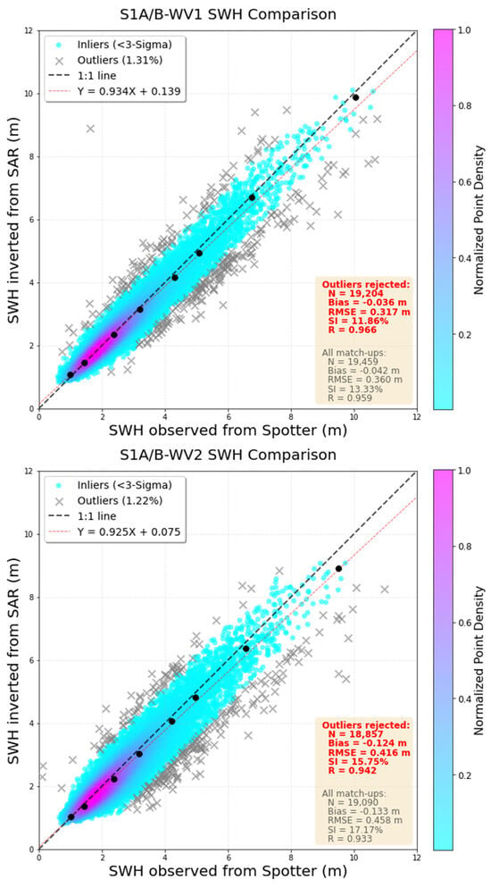
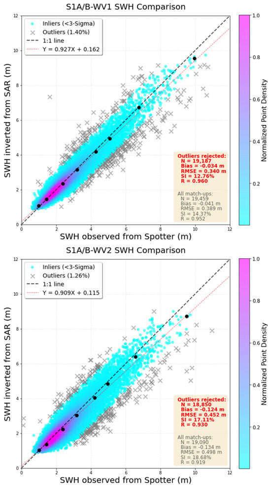
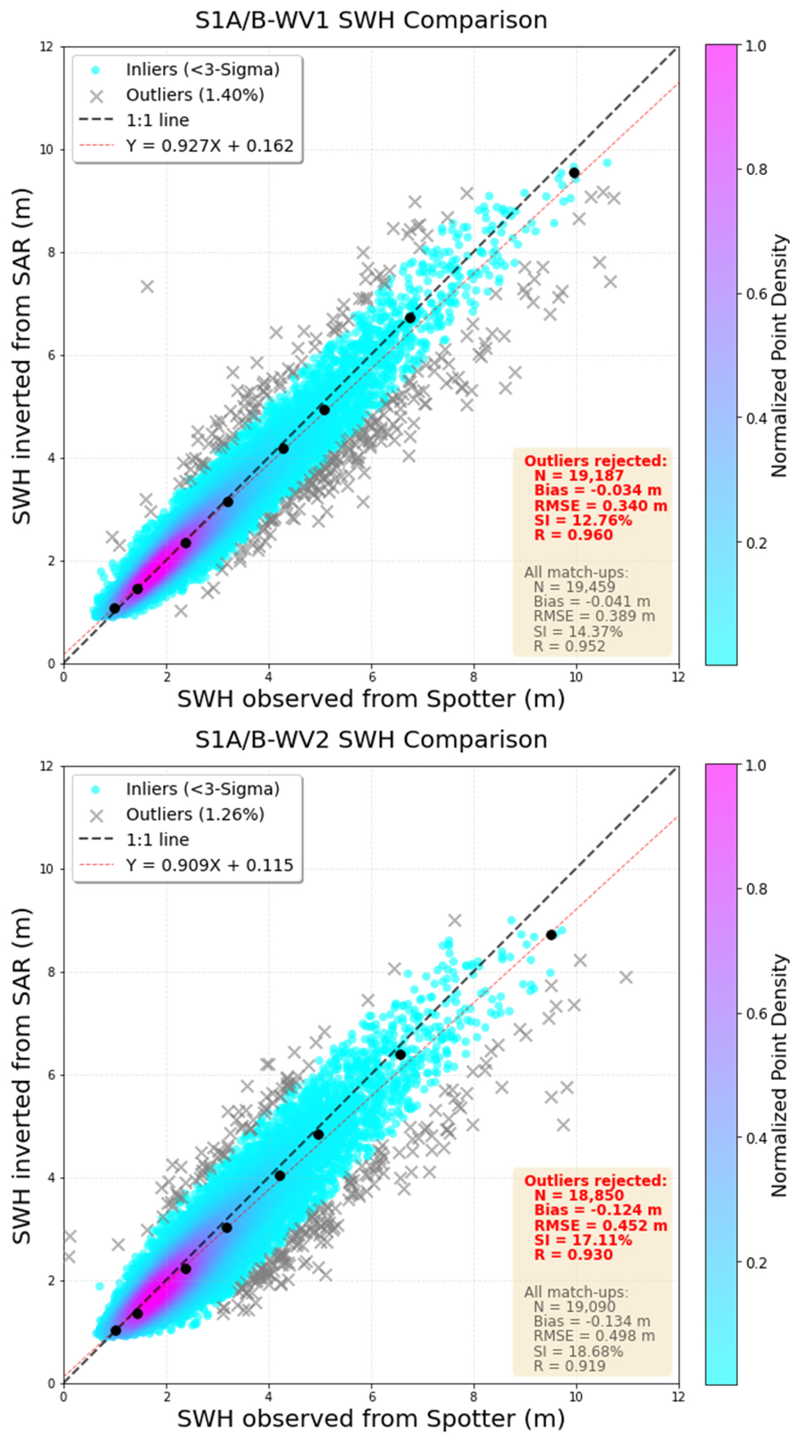
As shown in Figure 2, the scatter distributions are concentrated around the one-to-one reference line, and the regressions are close to unity, indicating good agreement between SAR retrievals and Spotter in situ observations over the SWH range approximately 0.5–10.0 m. Based upon the complete SAR–Spotter set, the RMSEs of 0.36 m and 0.45 m are presented for WV1 and WV2, respectively, against Spotter drifters. Here, few outliers were identified using a 3σ-based residual criterion. It should be noted that this slight proportion (approximately 1%) of matchups is mainly attributed to the imperfectness of spatiotemporal collocation within the adopted window (1 h and 100 km), during which wave conditions may evolve or vary substantially even over open oceans. In addition, Sentinel-1 SAR could be considered as spatially integrated observations over a 20 × 20 km imagette instantaneously, whereas a Spotter buoy measures waves at a single point over a one-hour time period, so representativeness differences between the two observing systems can also contribute to these anomalous discrepancies. After rejecting these 1% outliers, the proposed model achieves a bias of −0.036 m (−0.124 m), an RMSE of 0.317 m (0.416 m), an SI of 11.86% (15.75%), and a correlation coefficient of 0.966 (0.942) for WV1 (WV2). A small but discernible performance degradation is observed for the higher incidence from WV2 beam, which is similar to those of previous studies (e.g., [4,13]).

Figure 2. Comparisons of the Sentinel-1A/B SAR SWH retrievals against Spotter for (top) WV1 and (bottom) WV2. The color shading denotes the normalized point density of the inlier matchups retained after the 3σ-based outlier screening, while gray crosses denote outliers. The black dashed line represents the 1:1 line, and the red dashed line indicates the linear regression fit for the retained inlier. The black dots represent the quantile–quantile points for 1%, 10%, 50%, 75%, 90%, 95%, 99% and 99.99%. Statistical metrics calculated using the inlier. (All) Matchups are shown in red (gray).

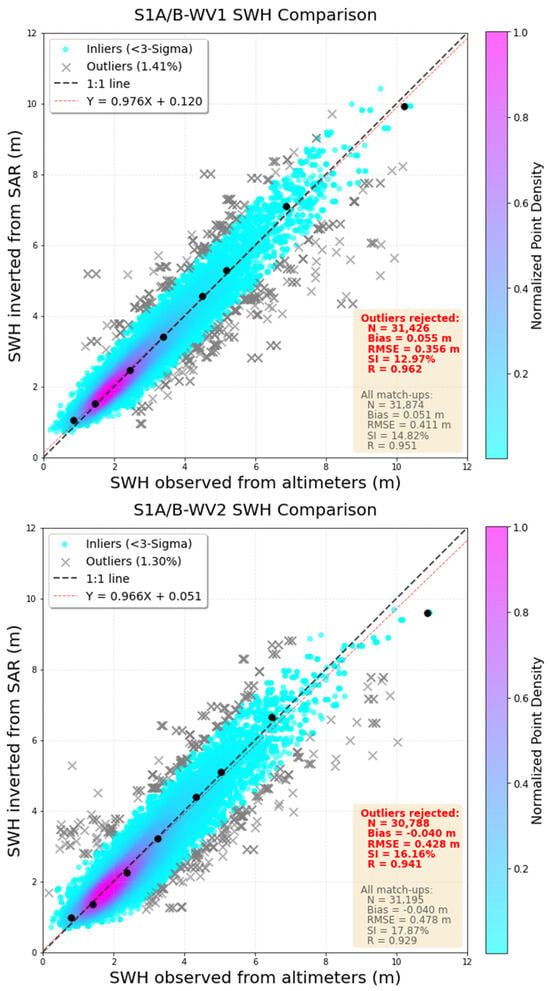
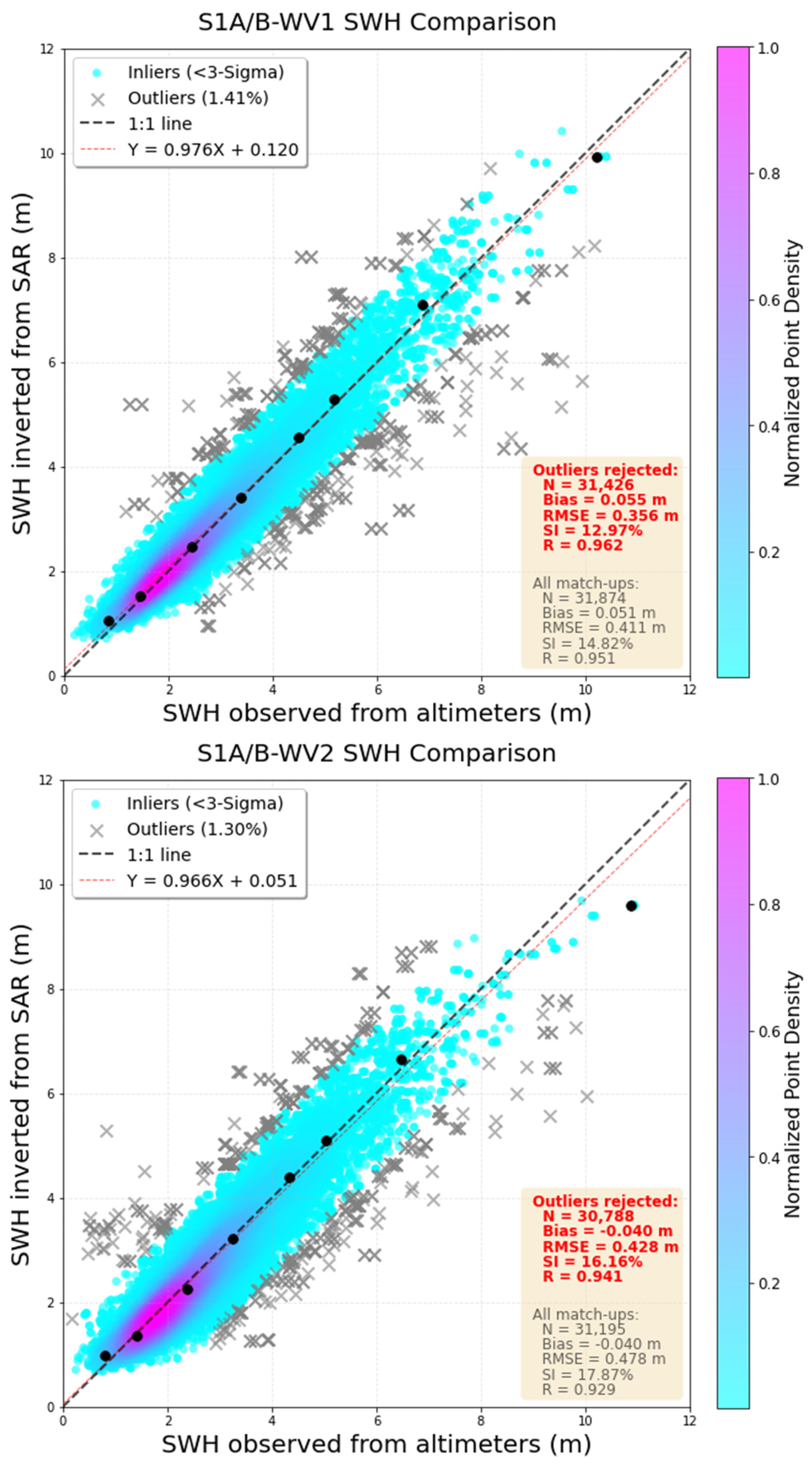
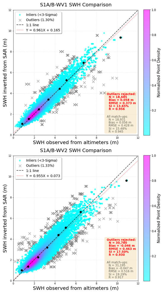
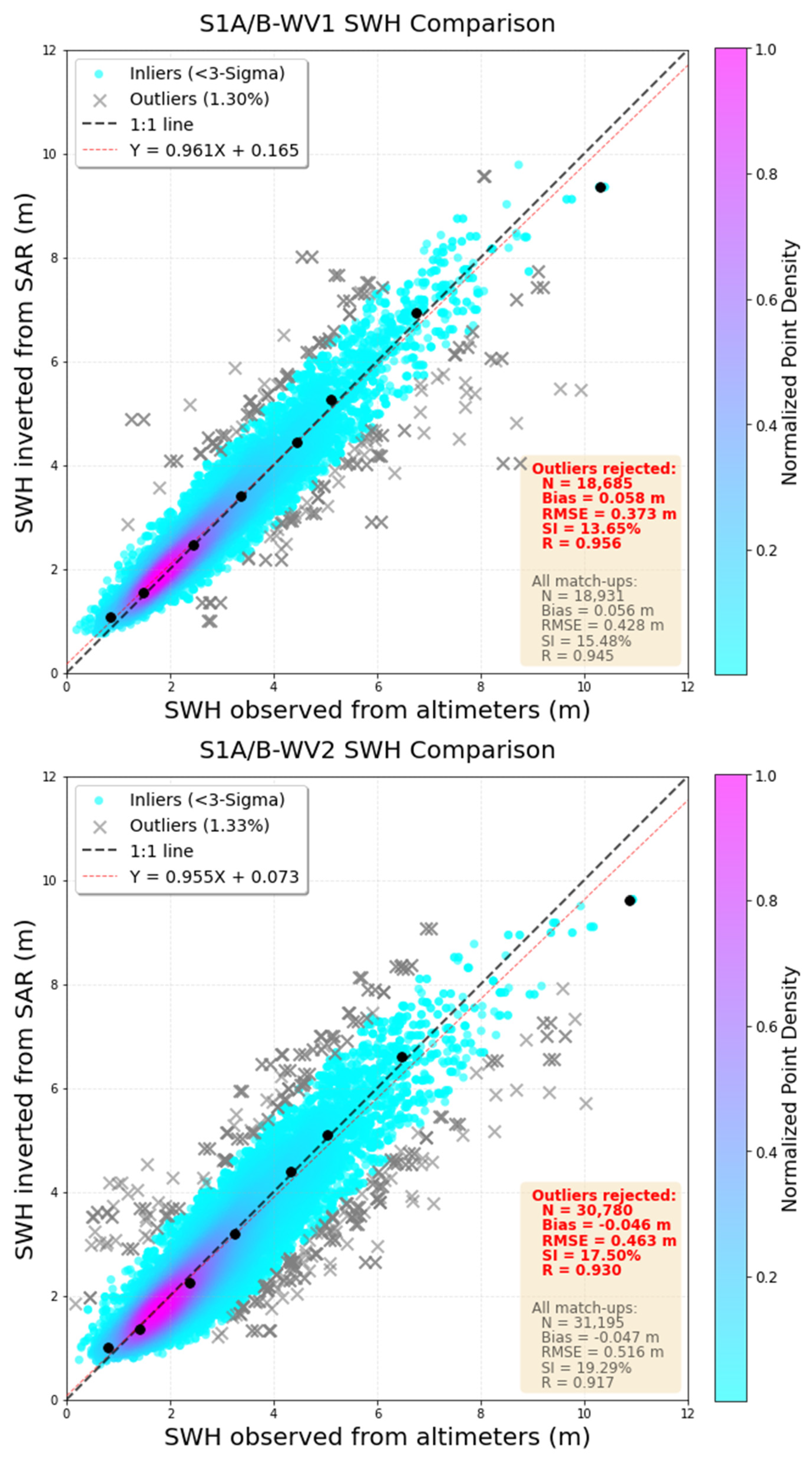
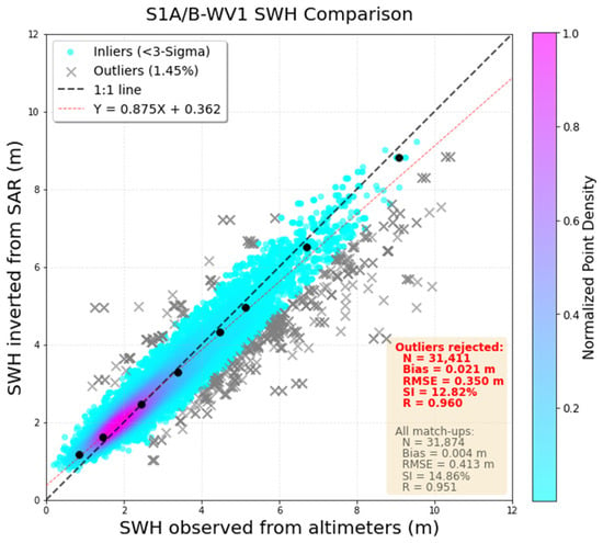
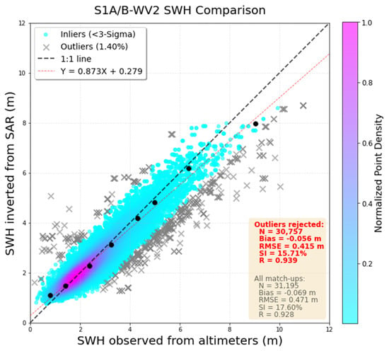
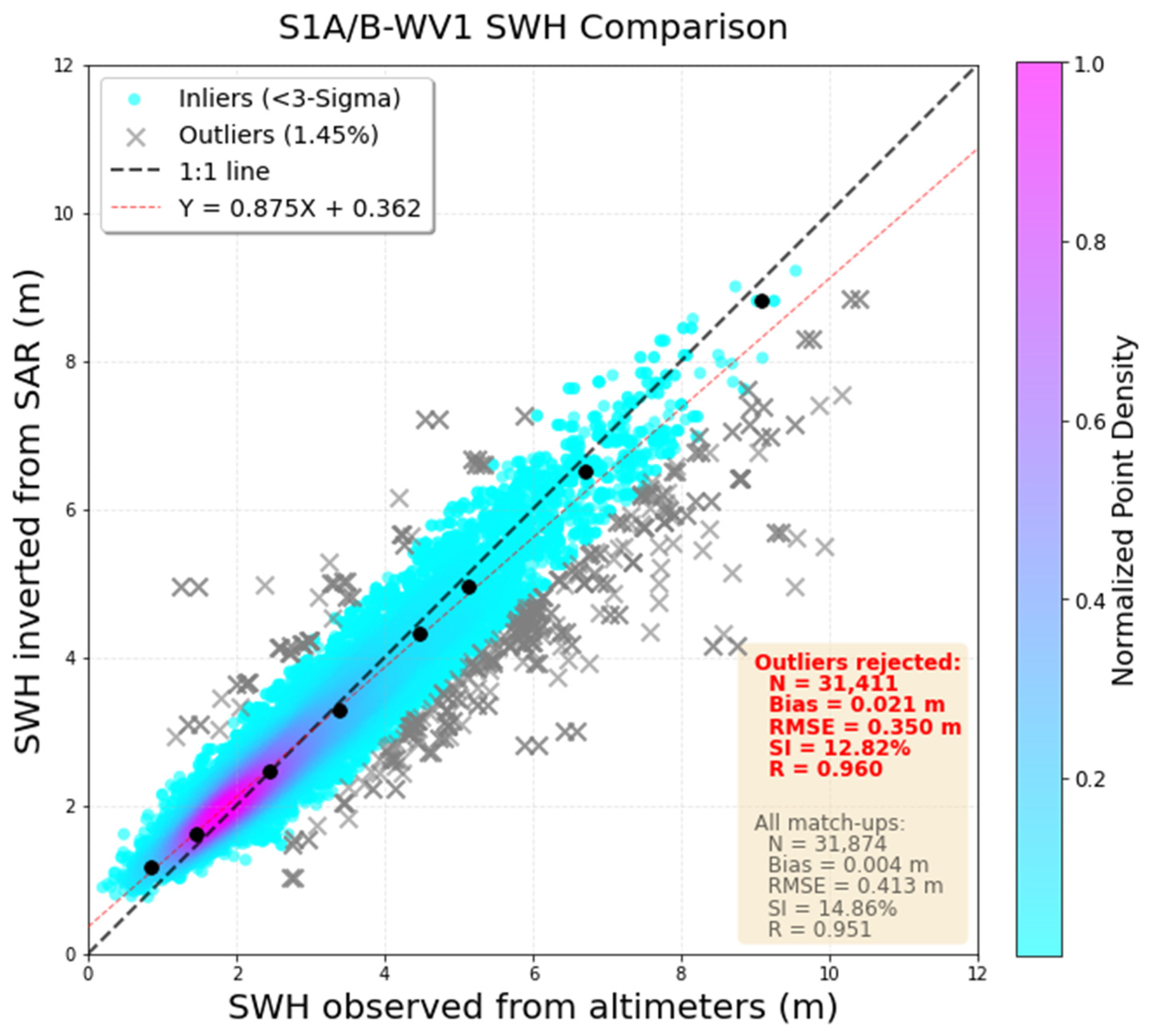
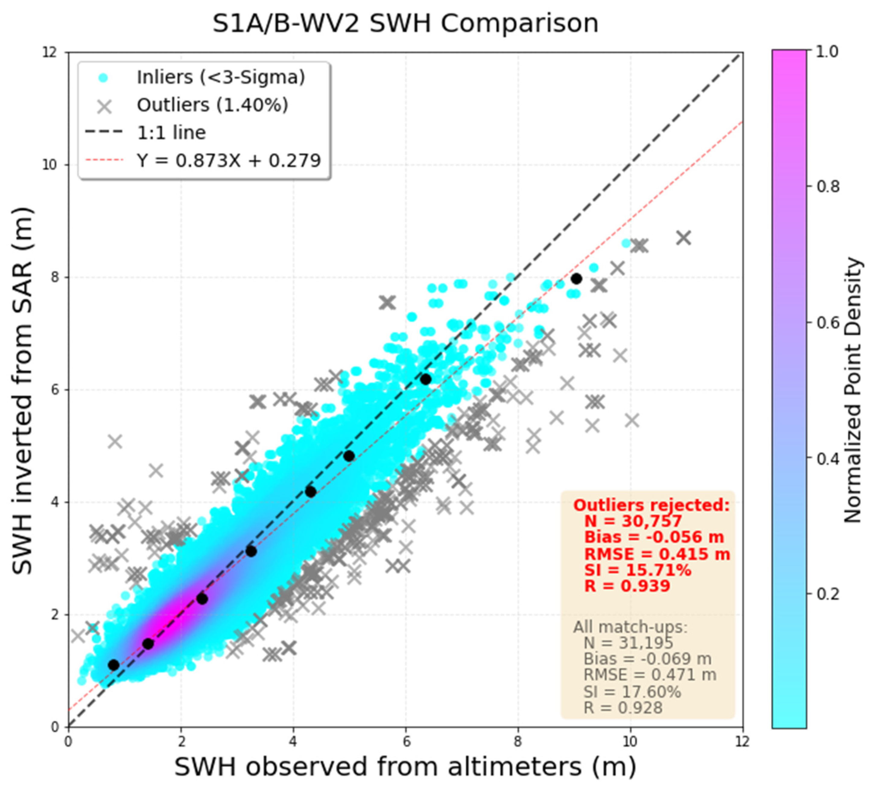
We also perform another independent validation against SWH measurements derived from multiplatform altimeters (i.e., Jason-3, SARAL and Sentinel-6) during the year of 2021. As shown in Figure 3, the altimeter-based verification exhibits scatter patterns similar to those obtained from the Spotter buoy validation (Figure 2). Also, the error metrics are close to those obtained from the Spotter validation, further confirming the robustness of our XGBoost-based retrieval model.

Figure 3. Same as Figure 2 but for independent validation of the XGBoost-derived Sentinel-1A/B SAR SWH against altimeter observations.

In addition, some quantiles (the 1st, 10th, 50th, 75th, 90th, 95th, 99th, and 99.99th) are specifically selected and represented by the black circles in both Figure 2 and Figure 3. These illustrate the consistency between our SAR-retrieved and buoy- and altimeter-observed SWH across different sea states, including high sea states (>8 m). In particular, the underestimation under extreme sea states appears to be alleviated, as suggested by the regression slopes, which are closer to unity in this study (0.93 and 0.97 against Spotter and altimeters, respectively) than the slope of 0.83 which was reported by the previous study [19].

In the literature, Quach et al. [19] reported a deep-learning-based Sentinel-1 WV SWH retrieval RMSE of approximately 0.53 m against a buoy in situ, and about 0.31 m against altimeter measurements. Yang et al. [22] developed a dual-branch convolutional neural network to retrieve SWH from Sentinel-1 WV with RMSE of 0.43 m compared to Copernicus Marine Environment Monitoring Service reanalysis. Recently, Pleskachevsky et al. [17] processed the complete archive of Sentinel-1 SAR in the scope of the ESA CCI program and reported SAR-retrieved SWH with RMSE of 0.40 m for WV1 and WV2 against buoys.

It should be noted that these error metrics may not be compared directly with the present RMSE (around 0.3–0.4 m via Spotter-based and altimeter-based assessments) because of differences in the reference dataset, matchup selection, quality control, and sea-state regime. These close error metrics still indicate that our proposed model can provide reliable estimates and achieve competitive accuracy performance comparable to recent deep-learning methods.

5. Discussion

5.1. Feature Importance and Model Interpretability

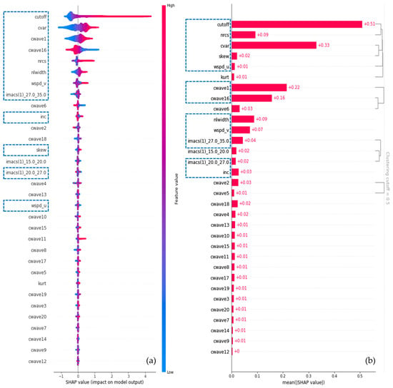
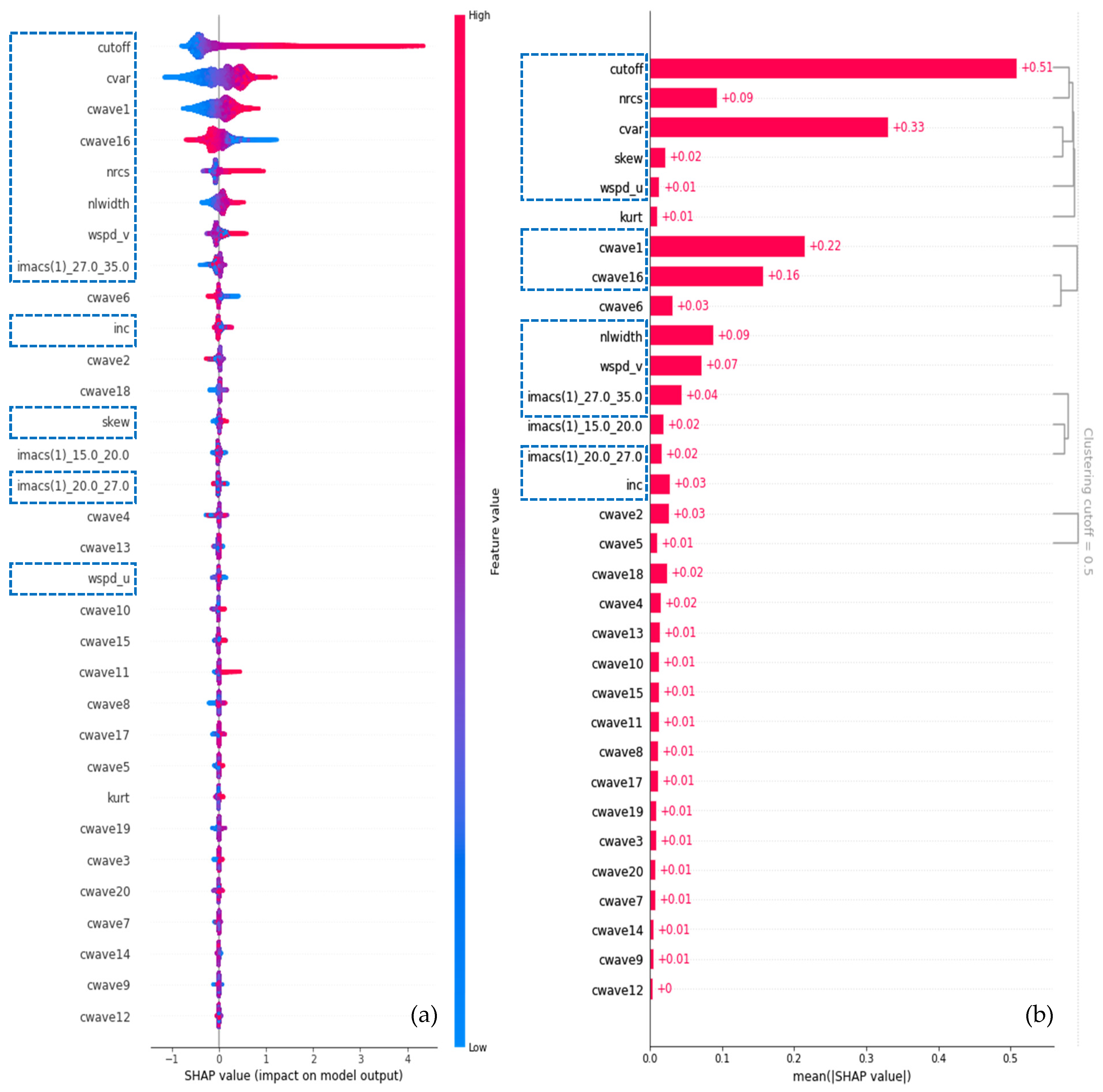
To further interpret the role of the input variables in the XGBoost retrieval model (see Table 2), SHAP analysis was conducted. SHAP provides an additive attribution framework in which the contribution of each feature to an individual prediction can be quantified. Figure 4a shows the SHAP summary plot, where the features are ranked according to their mean absolute SHAP values. The color indicates the original feature value, and the horizontal position represents the impact of that feature on the model output.

Figure 4. SHAP analysis of the XGBoost model. (a) SHAP summary plot illustrating the impact of each feature on model predictions. (b) SHAP-based hierarchical clustering, grouping variables with similar contributions. The blue dashed box represents the 12-feature inputs after filtering.

The azimuth cutoff wavelength, denoted as λ_c, is identified as the most influential predictor. This is physically reasonable because the azimuth cutoff is closely related to the velocity-bunching effect and nonlinear SAR imaging of ocean waves, and has long been recognized as a key parameter for SAR-based wave retrieval [6,48,49]. As shown in Figure 4a, a larger λ_c generally contributes positively to the retrieved SWH. This dependence is consistent with stronger azimuthal smearing under higher sea states (rather than demonstrative of it). The cvar is the second most important feature and represents the strength of SAR-image intensity modulation, which is closely associated with sea-surface roughness variability and wave-induced backscatter modulation. The NRCS also contributes substantially, which is consistent with the known sensitivity of radar backscatter to wind-induced short-wave roughness.

In contrast, most CWAVE parameters exhibit relatively small individual contributions. Only a limited number of components, such as cwave1 and cwave16, show notable importance, suggesting that the XGBoost model does not rely equally on all polynomial CWAVE descriptors. Instead, only specific CWAVE components provide useful information for representing the SAR image spectrum and its relationship with SWH. Similarly, the IMACS features contribute moderately and appear to provide complementary information related to multi-scale image modulation.

To account for potential redundancy among the input variables, SHAP-based hierarchical clustering was further applied, as shown in Figure 4b. Features were clustered using the pairwise distance d_ij = 1 − |ρ_ij|, where ρ_ij is the Pearson correlation between the SHAP values of features i and j. The dendrogram was cut at a distance of 0.5. This threshold was chosen by inspection of Figure 4b: it groups features with similar attribution patterns (|ρ| ≥ 0.5) while leaving the main physical families separate. A representative subset was then selected from each cluster. Within a cluster, the feature with the largest mean |SHAP| was retained. A second member was kept only when it encoded a complementary physical role (a different spectral scale or an orthogonal wind/geometry component); otherwise, the lower-ranked feature was discarded as redundant. Accordingly, the CWAVE parameters were reduced to cwave1 and cwave16, and the IMACS features to imacs(1)_20.0_27.0 and imacs(1)_27.0_35.0. Among the image statistics, cvar and skew were retained, whereas kurt was excluded because it clustered with these two variables and had a smaller mean |SHAP|. NRCS, λ_c, incidence angle, the two wind components, and nlwidth were preserved as cluster representatives or independent contributors. This procedure yielded the compact 12-feature set highlighted in Figure 4.

The XGBoost model was then retrained using the reduced feature set, with the optimized hyperparameters summarized in Table 3. As shown in Figure 5 and Figure 6, the retrained 12-feature compact model shows only a slight degradation (e.g., 0.02 m and 0.03 m degradation of RMSE against Spotter for WV1 and WV2, respectively) in retrieval accuracy compared with the full-feature model, indicating that the removed variables mainly provide redundant or marginal information. Therefore, the reduced model preserves the essential SAR SWH information while offering a more compact and interpretable representation. This reduction is beneficial not only for improving model transparency, but also for enhancing robustness and reducing the risk of overfitting when the model is applied to independent sensors or different sea-state conditions.

Figure 5. Same as Figure 2 but for validation of SWH derived from 12-feature compact XGBoost model against Spotter observations.

Figure 6. Same as Figure 3 but for validation of SWH derived from 12-feature compact XGBoost model against altimeter observations.

It should be noted that SHAP analysis provides a statistical attribution of model predictions rather than a direct causal interpretation. Nevertheless, the consistency between the statistical SHAP-derived feature importance and known physical SAR wave imaging mechanisms supports the interpretability of the proposed XGBoost-based retrieval framework.

5.2. Importance of QM Correction

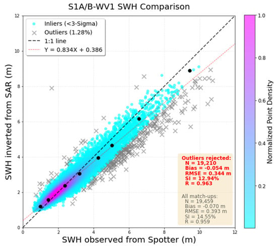
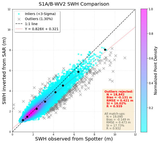
To assess the impact of the QM correction, the retrieval results obtained without QM correction, hereafter referred to as the raw-label results, were compared with buoy and altimeter observations, as shown in Figure 7 and Figure 8. Compared with the QM-corrected results shown in Figure 2 and Figure 3, the raw-label results exhibit larger biases and RMSEs, together with lower regression slopes, indicating systematic performance degradation for both WV1 and WV2.

Figure 7. Same as Figure 2 but for independent validation of the raw-label-trained XGBoost-derived Sentinel-1A/B SAR SWH against Spotter buoy observations.

Figure 8. Same as Figure 2 but for independent validation of the raw-label-trained XGBoost-derived Sentinel-1A/B SAR SWH against altimeter observations.

The uncorrected results overestimate low SWH and underestimate high SWH, and the fitted slopes fall well below unity (0.834 for WV1 and 0.828 for WV2; Table 4). After QM correction the slopes increase to 0.934 and 0.925, respectively, and the quantile–quantile points in Figure 2 and Figure 3 remain closer to the 1:1 line at both ends of the SWH range. The corresponding RMSE reduction is modest, especially for WV2 (0.421 m to 0.416 m; 0.344 m to 0.317 m for WV1). Thus, the principal benefit of QM is to restore retrieval scaling and dynamic range, although not to produce a large decrease in overall RMSE.

Table 4. Validation statistics of SAR-retrieved SWH against buoy observations for Sentinel-1A and Sentinel-1B.

Mode	WV1				WV2
SAR	S1A/B (QM)	S1A/B (RAW)	S1A	S1B	S1A/B (QM)	S1A/B (RAW)	S1A	S1B
Bias (m)	−0.036	−0.054	−0.032	−0.043	−0.124	−0.131	−0.109	−0.149
RMSE (m)	0.317	0.344	0.318	0.315	0.416	0.421	0.412	0.429
SI	11.86%	12.94%	11.75%	12.08%	15.75%	16.02%	15.45%	16.51%
R	0.966	0.963	0.966	0.967	0.942	0.939	0.940	0.942
N	19,459	19,459	12,053	7408	19,090	19,090	11,849	7244
Fit Line	Y = 0.934X +0.139	Y = 0.834X +0.386	Y = 0.928X +0.162	Y = 0.943X +0.105	Y = 0.925X +0.075	Y = 0.828X +0.321	Y = 0.927X +0.085	Y = 0.915X +0.071

5.3. Cross-Platform Consistency

To further evaluate the transferability of our model, the buoy-based validation results were separated for Sentinel-1A and Sentinel-1B, as summarized in Table 4. Although the model was trained exclusively using Sentinel-1A data, its performance on Sentinel-1B remains comparable.

For both WV1 and WV2, the accuracy metrics for Sentinel-1A and Sentinel-1B are highly consistent, with similar bias, RMSE, SI, and correlation values. The regression relationships also show no noticeable differences between the two sensors.

These results indicate that the model generalizes well across the Sentinel-1A and Sentinel-1B platforms and does not introduce significant sensor-dependent biases. Here, we emphasize, however, that this is an assessment of within-mission consistency rather than cross-platform generalization, since Sentinel-1A and Sentinel-1B are twin satellites sharing an identical instrument design.

5.4. Sensitivity to the Collocation Window

The SAR–Spotter validation uses a radius of 100 km and a search window of 1 h (Section 3.1). The radius follows the along-track sampling of the Sentinel-1 wave mode, about 200 km between successive acquisitions at the same incidence (Section 2.1), and is consistent with previous collocations of Sentinel-1 WV retrievals against buoys [4] and altimeters [19].

In fact, Spotter SWH is an hourly record [26]. Hence, matching each imagette to the nearest Spotter data limits the time difference to 30 min, though the nominal 1 h window is applied. Of the 38,549 pairs, the median separation is 69 km and only 27% lie within 50 km. The median time difference is 15 min, and none exceeds 30 min.

Table 5 recomputes the comparison on every matchup, without the 3σ screening used for the red metrics in Figure 2. The baseline RMSE is 0.36 m for WV1 and 0.46 m for WV2. Shortening the time limit to 15 min leaves these values unchanged. Reducing the radius to 50 km lowers the RMSE by about 0.03 m, and a 25 km radius lowers it by about 0.05 m. Bias and correlation remain essentially the same.

Table 5. SAR–Spotter errors for tighter collocation windows, using all matchups (no residual screening).

Window	WV1		WV2
	N	RMSE	N	RMSE
100 km/30 min	19,459	0.36 m	19,090	0.46 m
50 km/30 min	5281	0.33 m	5235	0.43 m
25 km/30 min	1298	0.31 m	1330	0.41 m
100 km/15 min	9831	0.37 m	9421	0.46 m

The 100 km window is retained for the primary validation. A 50 km subset keeps about a quarter of the pairs, and a 25 km subset, comparable to the 20 km imagette, leaves only seven (WV1) and three (WV2) cases with SWH ≥ 8 m, which is too few for the high-sea-state evaluation.

6. Conclusions

In this study, we have developed an explainable machine learning framework for retrieving SWH from Sentinel-1 SAR wave mode observations. By applying quantile-mapping correction using a collocated Spotter buoy in situ as reference, we effectively mitigated the sea-state-dependent biases inherent in ERA5 reanalysis SWH data. This approach enabled the construction of a large-scale, high-quality training dataset that combines the global coverage of reanalysis with the accuracy advantages of in situ observations. An XGBoost machine learning model was then trained on 32 physically meaningful SAR-derived features extracted from Sentinel-1 Level-2 OCN products, including image statistics (e.g., cvar, skewness, kurtosis), spectral parameters (CWAVE and IMACS), azimuth cutoff wavelength, NRCS, and wind-related information.

Comprehensive independent validations against Spotter-drifting-buoy and multi-mission altimeter (Jason-3, SARAL, Sentinel-6) observations throughout 2021 demonstrated the robustness and accuracy of the proposed model. The XGBoost model achieves RMSEs of 0.36 m (WV1) and 0.45 m (WV2), correlation coefficients of 0.959 (WV1) and 0.933 (WV2) and regression slope of 0.93 against the independent drifting Spotter buoy. After outlier rejection, the retrievals achieved lower RMSEs of 0.317 m (WV1) and 0.416 m (WV2). These results are competitive with the State-of-the-Art deep-learning approaches. Agreement at high sea states (SWH > 8 m) is suggested by the upper quantile–quantile points and regression slopes. Because such high-SWH matchups are few, this comparison is indicative rather than a separate tail-specific validation. SHAP analysis provided clear physical insights into model behavior, indicating that λ_c, cvar, and NRCS are the dominant predictors. A compact 12-feature model (selected via SHAP-based hierarchical clustering) retained nearly equivalent performance, enhancing both interpretability and computational efficiency.

The QM correction was shown to be essential: models trained on raw ERA5 labels exhibited systematic overestimation at low SWH and underestimation at high SWH, whereas QM-corrected labels reduced these systematic biases and restored the full dynamic range of retrievals. Furthermore, the model generalized well across Sentinel-1A and Sentinel-1B platforms despite being trained exclusively on Sentinel-1A data, demonstrating transferability between these two closely related platforms.

This work advances SAR-based SWH retrieval by integrating observation-adjusted reanalysis labels, accurate data-driven modeling, and explainability, thereby addressing key limitations of both conventional empirical algorithms and black-box machine-learning approaches. The proposed machine learning framework offers a reliable solution for global open-ocean SWH monitoring from Sentinel-1 SAR WV data, with promising applications in near-real-time ocean engineering services and long-term climate data records. Future efforts will explore its extension to SAR missions rather than Sentinel-1 constellation (e.g., Gaofen-3), working modes (coastal wide swath), and retrieval of additional wave parameters such as wave periods.

References

- Hasselmann, K.; Chapron, B.; Aouf, L.; Ardhuin, F.; Collard, F.; Engen, G.; Hasselmann, S.; Heimbach, P.; Janssen, P.; Johnsen, H.; et al. The ERS SAR Wave Mode: A Breakthrough in Global Ocean Wave Observations. In ERS Missions: 20 Years of Observing Earth; Fletcher, K., Ed.; European Space Agency: Noordwijk, The Netherlands, 2013; pp. 165–198. [Google Scholar]
- Li, X.M.; Huang, B.Q. A Global Sea State Dataset from Spaceborne Synthetic Aperture Radar Wave Mode Data. Sci. Data 2020, 7, 261. [Google Scholar] [CrossRef] [Scilit] [PubMed]
- Wang, H.; Mouche, A.; Husson, R.; Chapron, B. Indian Ocean Crossing Swells: New Insights from Fireworks Perspective Using Envisat Advanced Synthetic Aperture Radar. Remote Sens. 2021, 13, 670. [Google Scholar] [CrossRef] [Scilit]
- Stopa, J.E.; Mouche, A. Significant Wave Heights from Sentinel-1 SAR: Validation and Applications. J. Geophys. Res. 2017, 122, 1827–1848. [Google Scholar] [CrossRef] [Scilit]
- Hasselmann, K.; Raney, R.K.; Plant, W.J.; Alpers, W.; Shuchman, R.A.; Lyzenga, D.R.; Rufenach, C.L.; Tucker, M.J. Theory of Synthetic Aperture Radar Ocean Imaging: A MARSEN View. J. Geophys. Res. 1985, 90, 4659–4686. [Google Scholar] [CrossRef] [Scilit]
- Hasselmann, K.; Hasselmann, S. On the Nonlinear Mapping of an Ocean Wave Spectrum into a Synthetic Aperture Radar Image Spectrum and Its Inversion. J. Geophys. Res. 1991, 96, 10713–10729. [Google Scholar] [CrossRef] [Scilit]
- Hasselmann, S.; Brüning, C.; Hasselmann, K.; Heimbach, P. An Improved Algorithm for the Retrieval of Ocean Wave Spectra from Synthetic Aperture Radar Image Spectra. J. Geophys. Res. 1996, 101, 16615–16629. [Google Scholar] [CrossRef] [Scilit]
- Mastenbroek, C.; de Valk, C.F. A Semi-Parametric Algorithm to Retrieve Ocean Wave Spectra from Synthetic Aperture Radar. J. Geophys. Res. 2000, 105, 3497–3516. [Google Scholar] [CrossRef] [Scilit]
- Schulz-Stellenfleth, J.; Lehner, S.; Hoja, D. A Parametric Scheme for the Retrieval of Two-Dimensional Ocean Wave Spectra from Synthetic Aperture Radar Look Cross Spectra. J. Geophys. Res. 2005, 110, 297–314. [Google Scholar] [CrossRef] [Scilit]
- Sun, J.; Guan, C.L. Parameterized First-Guess Spectrum Method for Retrieving Directional Spectrum of Swell-Dominated Waves and Huge Waves from SAR Images. Chin. J. Oceanol. Limnol. 2006, 24, 12–20. [Google Scholar] [CrossRef] [Scilit]
- Schulz-Stellenfleth, J.; Konig, T.; Lehner, S. An Empirical Approach for the Retrieval of Integral Ocean Wave Parameters from Synthetic Aperture Radar Data. J. Geophys. Res. 2007, 112, 1–14. [Google Scholar] [CrossRef] [Scilit]
- Li, X.M.; Lehner, S.; Bruns, T. Ocean Wave Integral Parameter Measurements Using Envisat ASAR Wave Mode Data. IEEE Trans. Geosci. Remote Sens. 2011, 49, 155–174. [Google Scholar] [CrossRef] [Scilit]
- Wang, H.; Wang, J.; Yang, J.S.; Ren, L.; Zhu, J.; Yuan, X.; Xie, C. Empirical Algorithm for Significant Wave Height Retrieval from Wave Mode Data Provided by the Chinese Satellite Gaofen-3. Remote Sens. 2018, 10, 363. [Google Scholar] [CrossRef] [Scilit]
- Lehner, S.; Pleskachevsky, A.; Bruck, M. High-Resolution Satellite Measurements of Coastal Wind Field and Sea State. Int. J. Remote Sens. 2012, 33, 7337–7360. [Google Scholar] [CrossRef] [Scilit]
- Bruck, M.; Lehner, S. TerraSAR-X/TanDEM-X Sea State Measurements Using the XWAVE Algorithm. Int. J. Remote Sens. 2015, 36, 3890–3912. [Google Scholar] [CrossRef] [Scilit]
- Pleskachevsky, A.; Tings, B.; Wiehle, S.; Imber, J.; Jacobsen, S. Multiparametric Sea State Fields from Synthetic Aperture Radar for Maritime Situational Awareness. Remote Sens. Environ. 2022, 280, 113200. [Google Scholar] [CrossRef] [Scilit]
- Pleskachevsky, A.; Tings, B.; Schnupfhagn, C.; Wiehle, S.; Jacobsen, S. First Processing of the Complete Sentinel-1 SAR Archive-10 Years of Global Sea State. IEEE J. Sel. Top. Appl. Earth Obs. Remote Sens. 2026, 19, 10183–10200. [Google Scholar] [CrossRef] [Scilit]
- Li, X.; Xu, Q.; Wang, H.; Jiang, H.; Yin, X.; Mu, S.; Li, X.; Su, H.; Wang, A.; Yang, Y.; et al. AI in Satellite Remote Sensing of the Ocean. Proc. IEEE 2026, 114, 362–395. [Google Scholar] [CrossRef] [Scilit]
- Quach, B.; Glaser, Y.; Stopa, J.E.; Mouche, A.A.; Sadowski, P. Deep Learning for Predicting Significant Wave Height from Synthetic Aperture Radar. IEEE Trans. Geosci. Remote Sens. 2021, 59, 1859–1867. [Google Scholar] [CrossRef] [Scilit]
- Wu, K.; Li, X.M.; Huang, B. Retrieval of Ocean Wave Heights from Spaceborne SAR in the Arctic Ocean with a Neural Network. J. Geophys. Res. Ocean. 2021, 126, e2020JC016946. [Google Scholar] [CrossRef] [Scilit]
- Xue, S.; Geng, X.; Yan, X.H.; Xie, T.; Yu, Q. Significant Wave Height Retrieval from Sentinel-1 SAR Imagery by Convolutional Neural Network. J. Oceanogr. 2020, 76, 465–477. [Google Scholar] [CrossRef] [Scilit]
- Yang, H.; Ai, W.; Zhao, X.; Guo, C.; Liu, Z.; Hu, S. Retrieval of Significant Wave Height from Sentinel-1 Wave Mode Data Under Rainfall Conditions with Dual-Branch CNN. IEEE J. Sel. Top. Appl. Earth Obs. Remote Sens. 2025, 18, 26505–26514. [Google Scholar] [CrossRef] [Scilit]
- Wang, H.; Yang, J.; Lin, M.; Li, W.; Zhu, J.; Ren, L.; Cui, L. Quad-Polarimetric SAR Sea State Retrieval Algorithm from Chinese Gaofen-3 Wave Mode Imagettes via Deep Learning. Remote Sens. Environ. 2022, 273, 112969. [Google Scholar] [CrossRef] [Scilit]
- Sun, F.; Li, X.; Li, X.M.; Ren, Y.; Wu, K. Retrieval of Significant Wave Height in Coastal Seas of China from GaoFen-3 Satellites Based on Deep Learning. Remote Sens. 2026, 18, 966. [Google Scholar] [CrossRef] [Scilit]
- Leng, S.; Hao, M.; Shao, W.; Marino, A.; Jiang, X. A Technique for SAR Significant Wave Height Retrieval Using Azimuthal Cut-Off Wavelength Based on Machine Learning. Remote Sens. 2024, 16, 1644. [Google Scholar] [CrossRef] [Scilit]
- Raghukumar, K.; Chang, G.; Spada, F.; Jones, C.; Janssen, T.; Gans, A. Performance Characteristics of ‘Spotter’, a Newly Developed Real-Time Wave Measurement Buoy. J. Atmos. Ocean. Technol. 2019, 36, 1127–1141. [Google Scholar] [CrossRef] [Scilit]
- Wang, H.T.; Freise, C.B. Error Analysis of the Directional Wave Spectra Obtained by the NDBC 3-m Pitch-Roll Discus Buoy. IEEE J. Ocean. Eng. 1997, 22, 639–648. [Google Scholar] [CrossRef] [Scilit]
- O’Reilly, W.C.; Olfe, C.B.; Thomas, J.; Seymour, R.J.; Guza, R.T. The California Coastal Wave Monitoring and Prediction System. Coast. Eng. 2016, 116, 118–132. [Google Scholar] [CrossRef] [Scilit]
- Hersbach, H.; Bell, B.; Perrisford, P.; Hirahara, S.; Horányi, A.; Muñoz-Sabater, J.; Nicolas, J.; Peubey, C.; Radu, R.; Schepers, D.; et al. The ERA5 Global Reanalysis. Q. J. R. Meteorol. Soc. 2020, 146, 1999–2049. [Google Scholar] [CrossRef] [Scilit]
- Cao, C.; Bao, L.; Gao, G.; Liu, G.; Zhang, X. A Novel Method for Ocean Wave Spectra Retrieval Using Deep Learning from Sentinel-1 Wave Mode Data. IEEE Trans. Geosci. Remote Sens. 2024, 62, 1–16. [Google Scholar] [CrossRef] [Scilit]
- Wang, H.; Chen, Y.; Xu, Y.; Zhu, J.; Yang, J.; Lang, S.; Husson, R.; Chapron, B. Deep Learning Merge of 2-D Wave Spectra from Real and Synthetic Aperture Radars. IEEE Geosci. Remote Sens. Lett. 2025, 22, 1–5. [Google Scholar] [CrossRef] [Scilit]
- Wang, H.; Chen, Y.; Zhu, J.; Chang, J.; Fang, Y.; Huang, X.; Yang, J.; Chapron, B. Enhancing Directional Wave Spectra Retrieval from Sentinel-1A SAR Wave Mode under Strong Cut-Off Distortions via Prior-Knowledge-Integrated Machine Learning. Remote Sens. 2026, 18, 1703. [Google Scholar] [CrossRef] [Scilit]
- Wang, J.; Wang, Y. Evaluation of the ERA5 Significant Wave Height against NDBC Buoy Data from 1979 to 2019. Mar. Geod. 2022, 45, 151–165. [Google Scholar] [CrossRef] [Scilit]
- Houghton, I.A.; Smit, P.B.; Clark, D.; Dunning, C.; Fisher, A.; Nidzieko, N.J.; Chamberlain, P.; Janssen, T.T. Performance Statistics of a Real-Time Pacific Ocean Weather Sensor Network. J. Atmos. Ocean. Technol. 2021, 38, 1047–1058. [Google Scholar] [CrossRef] [Scilit]
- Lancaster, O.; Cossu, R.; Boulay, S.; Hunter, S.; Baldock, T.E. Comparative Wave Measurements at a Wave Energy Site with a Recently Developed Low-Cost Wave Buoy (Spotter), ADCP, and Pressure Loggers. J. Atmos. Ocean. Technol. 2021, 38, 1019–1033. [Google Scholar] [CrossRef] [Scilit]
- Zhao, Y.; Jiang, B.; Han, Q.; Xu, J.; Xu, Y.; Meng, J.; Fan, C.; Chen, P. Generalized Calibration of Directional Wave Height Spectra from Multiple SWIM Beams Using Deep Learning. IEEE Trans. Geosci. Remote Sens. 2026, 64, 5103913. [Google Scholar] [CrossRef] [Scilit]
- Canto, M.; Khan, S.; Young, I.; Ribal, A.; Jansen, P.; Hansen, J.; Aouf, L.; Hemer, M. Multiplatform Calibration and Validation of CFOSAT Ocean Surface Waves. Ocean Dyn. 2026, 76, 56. [Google Scholar] [CrossRef] [Scilit]
- Dodet, G.; Piolle, J.-F.; Quilfen, Y.; Abdalla, S.; Accensi, M.; Ardhuin, F.; Ash, E.; Bidlot, J.-R.; Gommenginger, C.; Marechal, G.; et al. The Sea State CCI Dataset v1: Towards a Sea State Climate Data Record Based on Satellite Observations. Earth Syst. Sci. Data 2020, 12, 1929–1951. [Google Scholar] [CrossRef] [Scilit]
- López-García, P.; Gómez-Enri, J.; Muñoz-Pérez, J.J. Accuracy assessment of wave data from altimeter near the coast. Ocean Eng. 2019, 178, 229–232. [Google Scholar] [CrossRef] [Scilit]
- Enayati, M.; Bozorg-Haddad, O.; Bazrafshan, J.; Hejabi, S.; Chu, X. Bias Correction Capabilities of Quantile Mapping Methods for Rainfall and Temperature Variables. J. Water Clim. Change 2021, 12, 401–419. [Google Scholar] [CrossRef] [Scilit]
- Nguyen, N.Y.; Anh, T.N.; Nguyen, H.D.; Dang, D.K. Quantile Mapping Technique for Enhancing Satellite-Derived Precipitation Data in Hydrological Modelling: A Case Study of the Lam River Basin, Vietnam. J. Hydroinform. 2024, 26, 2026–2044. [Google Scholar] [CrossRef] [Scilit]
- Kazeminezhad, M.H. Neural Network-Enhanced Calibration of ERA5 Wind Speeds in the Northwestern Indian Ocean Using 32 Years of Satellite Observations. Remote Sens. Appl. Soc. Environ. 2026, 41, 101826. [Google Scholar] [CrossRef] [Scilit]
- Bessonova, V.; Tapoglou, E.; Dorrell, R.; Dethlefs, N.; York, K. Global Evaluation of Wave Data Reanalysis: Comparison of the ERA5 Dataset to Buoy Observations. Appl. Ocean Res. 2025, 157, 104490. [Google Scholar] [CrossRef] [Scilit]
- Timmermans, B.; Shaw, A.G.P.; Gommenginger, C. Reliability of Extreme Significant Wave Height Estimation from Satellite Altimetry and In Situ Measurements in the Coastal Zone. J. Mar. Sci. Eng. 2020, 8, 1039. [Google Scholar] [CrossRef] [Scilit]
- Chen, T.; Guestrin, C. XGBoost: A Scalable Tree Boosting System. In Proceedings ACM SIGKDD International Conference Knowledge Discovery and Data Mining; ACM: New York, NY, USA, 2016; pp. 785–794. [Google Scholar] [CrossRef] [Scilit]
- Li, H.; Chapron, B.; Mouche, A.; Stopa, J.E. A New Ocean SAR Cross-Spectral Parameter: Definition and Directional Property Using the Global Sentinel-1 Measurements. J. Geophys. Res. 2019, 124, 1566–1577. [Google Scholar] [CrossRef] [Scilit]
- Li, H.; Chapron, B.; Mouche, A.; Wang, C.; Lin, W.; He, Y. Ocean Surface Wind Wave Signatures in Single-Look Complex SAR Data. IEEE Trans. Geosci. Remote Sens. 2025, 63, 4203111. [Google Scholar] [CrossRef] [Scilit]
- Grieco, G.; Lin, W.; Migliaccio, M.; Nirchio, F.; Portabella, M. Dependency of the Sentinel-1 Azimuth Wavelength Cut-Off on Significant Wave Height and Wind Speed. Int. J. Remote Sens. 2016, 37, 5086–5104. [Google Scholar] [CrossRef] [Scilit]
- Corcione, V.; Grieco, G.; Portabella, M.; Nunziata, F.; Migliaccio, M. A Novel Azimuth Cutoff Implementation to Retrieve Sea Surface Wind Speed from SAR Imagery. IEEE Trans. Geosci. Remote Sens. 2019, 57, 3331–3340. [Google Scholar] [CrossRef] [Scilit]
Disclaimer/Publisher’s Note: The statements, opinions and data contained in all publications are solely those of the individual author(s) and contributor(s) and not of MDPI and/or the editor(s). MDPI and/or the editor(s) disclaim responsibility for any injury to people or property resulting from any ideas, methods, instructions or products referred to in the content. |
© 2026 by the authors. Licensee MDPI, Basel, Switzerland. This article is an open access article distributed under the terms and conditions of the Creative Commons Attribution (CC BY) license.