


Highlights
Retrieval methods for Sea Ice Concentration (SIC) and Sea Ice Thickness (SIT) during the Arctic freezing period are proposed using spaceborne GNSS-R data from the Tianmu-1 constellation. The XGBoost algorithm is employed with DDM-derived feature parameters as inputs to conduct SIC and SIT retrievals for the entire freezing period.
What are the main findings?
- An XGBoost-based framework for retrieving SIC and SIT from Tianmu-1 GNSS-R data.
- Daily SIC and SIT results throughout the 2023–2024 freezing period.
What is the implication of the main finding?
- First demonstration of Tianmu-1’s feasibility for sea ice retrieval, validating it as a new data source for polar monitoring.
- The comparative analysis of four GNSS systems Global Positioning System (GPS), BeiDou (BDS), Galileo (GAL), and Glonass (GLO) and the robust daily retrieval capability provide methodological support for operational sea ice product development.
Abstract
Sea ice concentration (SIC) and thickness (SIT) are critical variables for polar research. In this study, the potential of Tianmu-1 GNSS-R observations for retrieving Arctic SIC and SIT is explored using machine learning algorithms. XGBoost demonstrated superior accuracy and efficiency in the comparison of the three methods. For SIC retrieval, 14 parameters from Tianmu-1 were employed directly, whereas SIT retrieval incorporated additional auxiliary parameters, including SIC, sea ice salinity (S), and temperature (T). Among the different GNSS systems, GLO achieved the lowest RMSE for SIC, at 7.750%, whereas GAL performed comparatively poorly, with an RMSE of 10.475%. In SIT retrieval, the GPS and BDS yielded the smallest RMSE values of 0.276 m and 0.278 m, respectively, while GLO resulted in a slightly higher RMSE of 0.309 m. Daily retrievals of both the SIC and SIT were conducted from 18 October 2023 to 12 April 2024, with consistently stable evaluation metrics throughout the freezing season. In high-concentration regions, the retrieved SIC and SIT closely matched the reference data, whereas larger errors occurred in marginal ice zones and coastal areas. This study reveals the potential of Tianmu-1 to complement existing satellite missions in Arctic sea ice monitoring during the freezing period.
1. Introduction
As an important component of the cryosphere, the status of sea ice has a significant effect on the polar environment and global climate conditions. Consequently, monitoring its dynamic changes is essential for operational applications such as polar climate prediction and navigation support. Sea Ice Concentration (SIC) and Sea Ice Thickness (SIT) are two of the most critical sea ice parameters. As such, their precise retrieval represents a key research direction in ocean remote sensing. Global navigation satellite system reflectometry (GNSS-R) [1] is an emerging remote sensing technology. Due to its advantages such as passive reception, all-weather operation, and large-scale coverage, it has been widely applied in the field of ocean remote sensing in recent years, and has been successfully used in studies on global sea surface wind speed [2], global significant wave height [3], and sea ice monitoring [4]. The U.K.-DMC satellite [5], launched in September 2003, carried a GPS-R payload for the first time to conduct spaceborne GNSS-R measurements, confirming the feasibility of GNSS-R technology in ocean remote sensing. After processing the acquired reflected signals, the TDS-1 satellite launched by the United Kingdom in 2014 obtained many Delay Doppler Maps (DDMs) [6], which have been widely used in sea ice remote sensing research [4]. Since then, various countries and regions have developed satellites equipped with GNSS-R receivers for global detection. Currently, there are CYGNSS, SMAP GNSS-R, and Spire from the United States; 3Cat-2, 3Cat-5 A/B (FSSCat), and 3Cat-4 from Spain; PRETTY and HydroGNSS from the European Space Agency; TRITON (FORMOSAT-7R) from Taiwan; and the Fengyun-3 series, Jilin 01B, and Tianmu-1 from China [7]. Researchers have conducted extensive studies on the monitoring of polar sea ice through the large number of reflected signals obtained from these satellites for sea ice detection and the retrieval of SIC and SIT.
In published research, the accuracy of SIC retrieval has continuously increased with the application of different parameters and retrieval methods. Zhu et al. [8] proposed a model for estimating sea ice concentration based on the right-edge waveform sum (REWS) of differential delay waveforms (DDWs), which are features generated by the DDM from the TDS-1 satellite. The REWS-based model achieved retrieval accuracies with root mean square errors (RMSEs) of 11.78%/12.10% and biases of 1.67%/1.94% in the Northern and Southern Hemispheres, respectively. Llaveria et al. [9] utilized combined data from the microwave radiometer (MWR) and GNSS-R of the FSSCat mission to propose a neural network (NN) method for generating sea ice concentration and coverage products. The mean absolute errors (MAEs) of the generated SIC maps were 3.57% and 1.95% in the Antarctic Ocean and Arctic Ocean, respectively. Yan et al. [10] used an NN-based method to process DDMs and achieved a high-precision estimation of SIC with a correlation coefficient (R) exceeding 90%. They subsequently constructed a convolutional neural network (CNN) model [11] to retrieve the SIC at the specular point (SP) by processing the DDMs as images, which increased R to 92%. A support vector regression (SVR) algorithm [12] was subsequently used to construct an SIC retrieval model based on features extracted from the DDM. Compared with the results of the previous NN and CNN models, the SVR retrieval results were more accurate, with an R of 94% and an RMSE of only 14.7%. Yang et al. [13] proposed an intelligent retrieval method based on deep neural networks (DNNs) that incorporates sea ice and ocean interactions into the model. Compared with the SIC product from the University of Hamburg, the retrieval results from March and June 2016 were highly consistent and had small deviations, with RMSEs of 2.84% and 4.15%, respectively. Wang et al. [14] proposed a method to estimate high-temporal resolution and high-spatial resolution SIC by combining DDM parameters and sea surface temperature (SST) data using the LightGBM algorithm. The R obtained with the OSI SAF product reached 96.5%, with MAE and RMSE values of 6.1% and 9.0%, respectively.
The retrieval of SIT using GNSS-R techniques has been explored and developed through various methodological approaches. Li, Cardellach et al. [15] reported in preliminary experiments on sea ice thickness that the signals received by the TDS-1 satellite were reflected mainly from the sea ice–seawater interface, with an RMSD of 0.047 m at a phase delay observation value of 20 ms, demonstrating the potential of TDS-1 satellite signals for SIT retrieval. By considering only coherent GNSS reflections, Yan and Huang developed a double-layer (sea ice–seawater) empirical model to retrieve SIT [16]. They derived the reflectivity () of sea ice–seawater from the power received at the specular point on the basis of the Fresnel reflection coefficient and propagation loss of sea ice and obtained root mean square difference (RMSD) values of 0.0939 m compared with SMOS and 0.0949 m compared with SMOS/SMAP. They also retrieved SIT data using the scattering coefficient ( °) produced by TDS-1 [17], and the results were compared with those from the SMOS SIT, yielding an RMSD of 0.0868 m. Since this model requires external data to calculate the ice thickness, Xie and Yan [18] established a practical semiempirical model to simplify the estimation of SIT and reduce the dependence on external auxiliary data. They used only FY-3E GNSS-R data to independently retrieve SIT, and the RMSE of the GPS test data was 0.1442 m, whereas that from the BDS was 0.1289 m. However, these studies were limited to thicknesses of less than 1 m. Munoz-Martin et al. [19] used the two-layer model [16] to extend the work toward thicker sea-ice shelves and multiyear sea-ice shelves and to investigate the effect of fully polarimetric GNSS-R reflectivity on SIT changes. The results were highly consistent with the CS2SMOS SIT data.
Recently, machine learning algorithms have been increasingly used in SIT retrieval. Herbert et al. [20] constructed a regression neural network model using brightness temperature data from the FSSCat mission and auxiliary data, generating weekly composites of the Arctic SIT and monthly maps of the Antarctic. Yan and Huang [21] used two methods, namely, convolutional neural networks (CNNs) and support vector regression (SVR), to estimate the SIT. The inputs for the two models included the scattering coefficient ( °), incidence angle (), sea ice salinity (S) and temperature (T). The results revealed that the correlation coefficients for SVR and the CNN were 0.95 and 0.90, respectively, and the corresponding RMSEs were 0.0549 m and 0.0797 m, respectively. Li et al. [22] used the random forest (RF) regression method based on FY-3E data, with model inputs consisting of , , S and T. The results revealed a correlation coefficient of 0.91 and a mean absolute error of 0.032 m for the GPS and R and MAE values of 0.90 and 0.036 m for the BDS. Hu et al. [23] proposed a seamless stacking-based retrieval model for SIT, with inputs including features extracted from the DDM, °, , S and T. Four base learners, a decision tree (DT), K-nearest neighbors (KNNs), SVR, and RFs, were used to construct the ensemble model. The retrieval results for thicknesses less than 1 m were validated using SMOS data, and the RMSE decreased to 0.4 m while R increased to 0.99. Thicknesses greater than 1 m also demonstrated strong agreement with the Cryosat-2 data, with a bias of −0.03 m and an ubRMSD of 0.74 m.
The Tianmu-1 constellation, China’s first low-Earth orbit meteorological satellite system built under a commercial model, was first launched on 14 October 2021. Currently, 23 satellites are operational in orbit, supporting four major navigation systems, namely, Global Positioning System (GPS), BeiDou (BDS), Galileo (GAL), and Glonass (GLO). Owing to its constellation-based operation, it provides a large volume of observational data with high observational density, enabling real-time, all-weather acquisition of global atmospheric, surface, and sea surface characteristic parameters. As delineated in Refs. [24,25,26,27], the contemporary applications of Tianmu-1 GNSS-R data are thoroughly expounded in remote sensing.
In this study, we explored the application of GNSS-R data acquired by the Tianmu-1 constellation in sea ice remote sensing. The primary innovation of this work lies in the comprehensive assessment of Tianmu-1 GNSS-R data for Arctic winter sea ice monitoring, specifically focusing on both sea ice concentration and thickness retrieval. Beyond providing one of the first systematic evaluations of Tianmu-1 GNSS-R data for this purpose, this work demonstrates the capability to retrieve both sea ice concentration and thickness on a daily basis with Arctic-wide coverage throughout the freezing season. Such continuous daily retrievals enable a more complete representation of winter sea ice evolution than is currently available from most existing single-source sea ice thickness products. On the basis of machine learning methods, we selected some of the DDM parameters from Tianmu-1 and auxiliary data to retrieve the SIC and SIT values, respectively. The significance of this research is underscored by the comparative analysis of four different GNSS systems (GPS, BDS, GAL, GLO), providing valuable insights into their respective performances for sea ice retrieval applications. In addition, we performed daily SIC and SIT retrievals across the entire 2023–2024 winter period, enabling a robust evaluation of the temporal stability and operational potential of the proposed approach. Section 2 introduces the research data and the preprocessing procedures. Section 3 presents the retrieval method used in this study. The results of the retrieval are analyzed in Section 4. The errors and feature importance are discussed in Section 5. Section 6 summarizes this paper and explores future research directions.
2. Data
2.1. Tianmu-1
The GNSS-R Level-1 data of Tianmu-1 provide corresponding raw DDM data, numerous feature parameters calculated by the DDM, specular point information, and information related to the signal transmitter and signal receiver at each observation point. This study used these parameters to retrieve the SIC and SIT values for the entire freeze period from October 2023 to April 2024. Considering that the TM11–TM22 satellites of Tianmu-1 were launched successively after December 2023, only the data from the TM01–TM10 satellites were available before that period. Additionally, the polarization modes of the TM01–TM10 and TM11–TM22 satellites differ [24]. The TM01–TM10 satellites use conventional left-hand circular polarization (LHCP) antennas only, whereas TM11 receives two orthogonal linearly polarized signals and TM12–22 receive both LHCP and right-hand circular polarization (RHCP) signals, leading to inherent differences in the recorded signal characteristics. To ensure dataset consistency and avoid introducing biases from differing polarization responses, the GNSS-R L1 data from the TM01–10 satellites were selected for the entire freeze period. The data are provided in HDF format and can be accessed at the website (https://www.tmsats.com/openSource (accessed on 1 September 2024)).
2.2. Reference Data
To retrieve the SIC, we adopt the daily SIC product from the EUMETSAT Ocean and Sea Ice Satellite Application Facility (OSISAF) as the reference dataset [28]. The OSISAF SIC product is derived from Special Sensor Microwave Imager Sounder (SSMIS) passive microwave observations, with a temporal resolution of 1 day and a spatial resolution of 10 km.
For the SIT, we used the CryoSat-2/SMOS (CS2SMOS) merged SIT product released by the Alfred Wegener Institute (AWI). The CS2SMOS SIT product is generated by merging SIT estimates from CryoSat-2 (CS2) radar altimeter data [29] with SIT retrievals from Soil Moisture and Ocean Salinity (SMOS) radiometer brightness temperatures [30]. The CS2-derived SIT data are less reliable in thin ice regions (<1 m) and at the ice edge, whereas the SMOS-derived SIT data exhibit greater uncertainty in thick ice areas (>1 m). Leveraging the complementary sensitivities of the two datasets, AWI fuses them to provide pan-Arctic weekly SIT estimates, which are available as a daily product with a spatial resolution of 25 km [31,32].
2.3. Auxiliary Data
Previous studies have shown that, in addition to GNSS-R data, auxiliary parameters such as sea ice salinity (S) and surface temperature (T) can substantially improve SIT retrieval accuracy [21,22]. Tian-Kunze et al. [30] derived S and T while iteratively retrieving thin ice thickness from SMOS brightness temperatures. These two parameters are provided in the SMOS L3 product, which has a temporal resolution of 1 day and a spatial resolution of 12.5 km. To analyze the retrieval results for different types of sea ice, this study utilized the OSI-403-d Global Sea Ice Type product from OSISAF [33]. This dataset provides daily averaged sea ice type information on a 10 km Lambert Azimuthal Grid.
2.4. Data Filtering and Matching
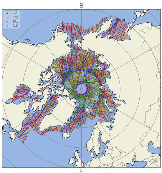
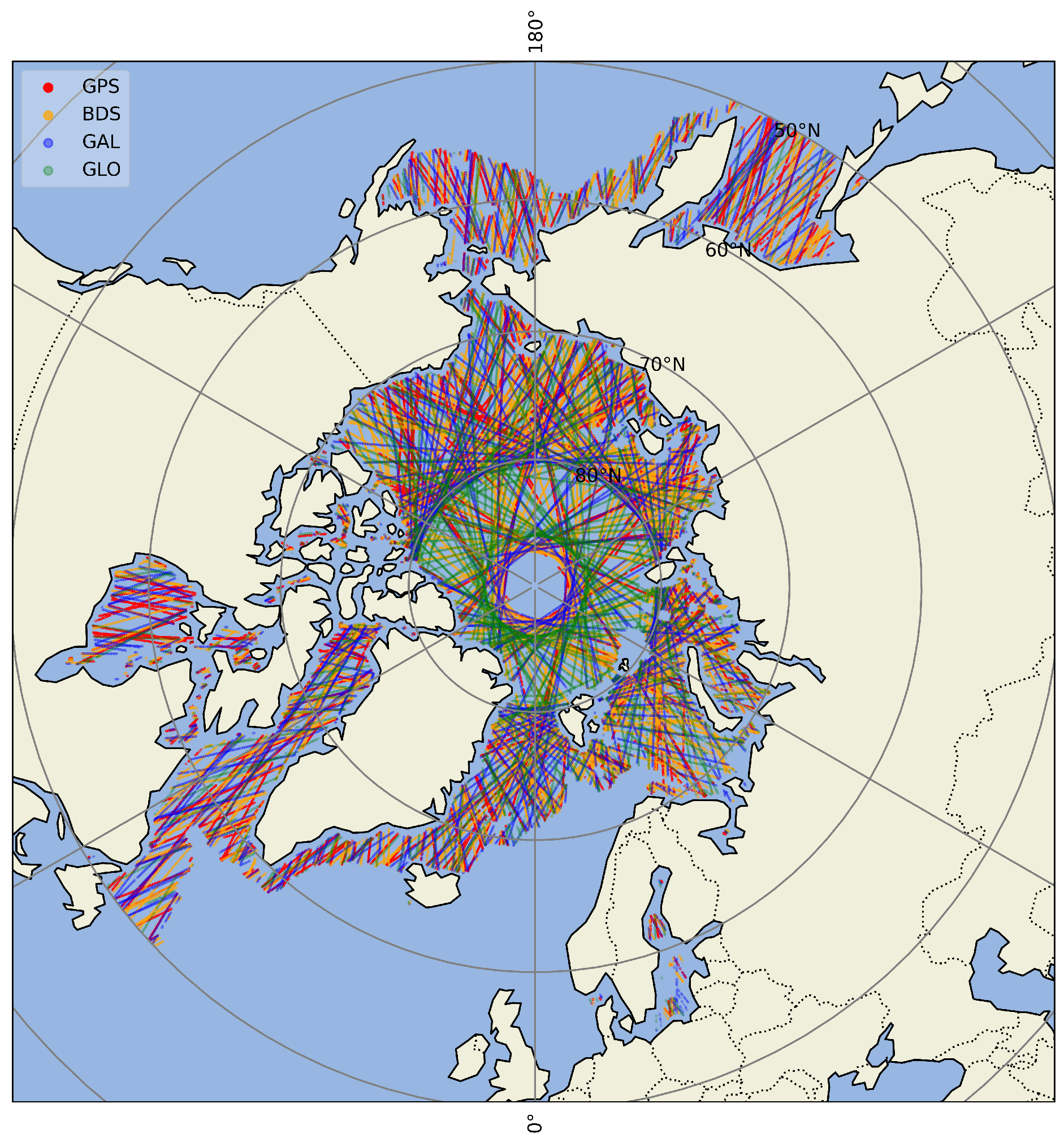
Tianmu-1 observations cover the global surface daily, but our focus is on Arctic sea ice. We therefore retained only specular points with latitudes above 50 °N. In the Tianmu-1 GNSS-R L1 data, the field Sp_surface_type indicates the surface type at the specular point: 0 indicates the open ocean, 0.5 indicates the coastal ocean within 25 km from land, 1 indicates land, and 2 indicates sea ice. Since our retrieval targets are the SIC and SIT, we keep only data where the surface type is labeled 2. Figure 1 shows the sea ice detection tracks of Tianmu-1 TM01–TM10 on 9 February 2024.
Figure 1.
Distribution of specular points from Tianmu-1 GNSS-R observations on 9 February 2024. Points are colored by their source GNSS system: GPS (red), BDS (orange), GAL (blue), and GLO (green).
DDM observations are occasionally affected by interference, and some are contaminated. The Ddm_quality_flag field in the Tianmu-1 L1 dataset provides a 20-bit binary quality flag. When any bit is set to 1, the quality of the DDM is damaged in some aspects (details in Ref. [25], Table 1). Only DDMs with all bits set to 0 (decimal value 0) are considered valid.
Table 1.
Feature parameters from Tianmu-1 GNSS-R data selected for SIC and SIT retrieval. Bold text indicates features used in both SIC and SIT retrieval.
The Tianmu-1 data were spatially and temporally matched with reference and auxiliary datasets. Given that all reference and auxiliary products have a daily temporal resolution, we assumed that SIC, SIT, S, and T remained constant within a day and matched records by date. OSISAF, CS2SMOS, and SMOS data are provided as gridded products, whereas Tianmu-1 data are point-based at the specular points. The nearest-neighbor interpolation method [34] was applied to collocate the Tianmu-1 observations with the reference data. Temporally, the data were matched on a daily basis. Spatially, for each GNSS-R reflection point, the value from the corresponding reference product’s grid cell that was geographically closest to the point’s location was assigned. This process formed the unified experimental dataset for this study.
3. Method
3.1. DDM Parameters Selection
The GNOS-M instrument onboard the TM-1 satellites receives GNSS signals reflected from the ocean surface, enabling the retrieval of sea surface properties relevant to sea ice detection. Due to the roughness of the ocean surface, the reflected GNSS signals are dominated by diffuse scattering, which gives rise to multiple signal components at the receiver. These multipath components result from differences in propagation paths and the relative motion between the reflecting surface and the receiving platform, producing distinct time delays and Doppler frequency shifts. Consequently, the reflected signal power can be expressed as a delay–Doppler function. This relationship is described by Equation (1), which provides a theoretical basis for characterizing the backscattered power distribution of different surface scattering targets [24,35,36]:
where is the reflected signal power as a function of delay and Doppler frequency , is the coherent integration time, is the transmitted signal power, and is the GNSS signal wavelength. and denote the transmitter and receiver antenna gains, and are the distances from the surface scattering element to the transmitter and receiver, respectively, x is the delay–Doppler ambiguity function, and represents the elemental scattering area.
Based on the DDM power formulation in Equation (1), two commonly used observables can be derived from the reflected GNSS signal. The normalized bistatic radar cross section (NBRCS) is defined as
and the reflectivity is given by
where denotes the averaged DDM power at the specular point, is the DDM peak power, and represents the effective scattering area.
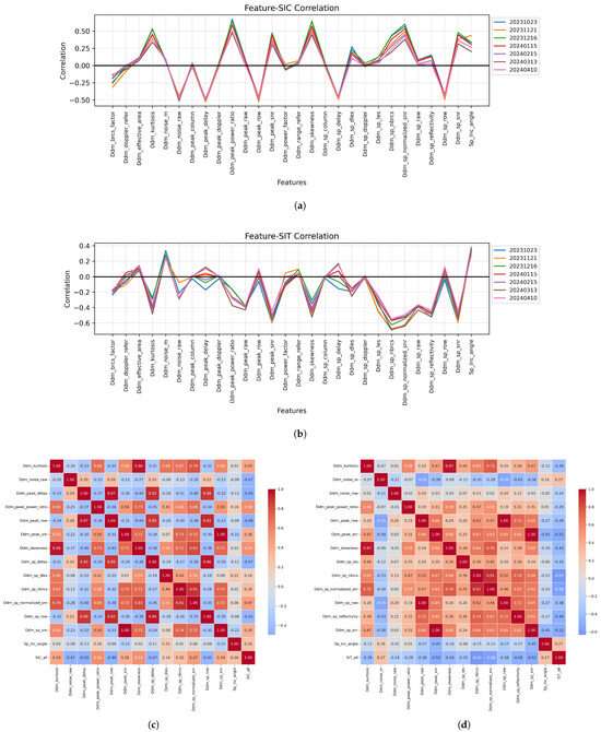
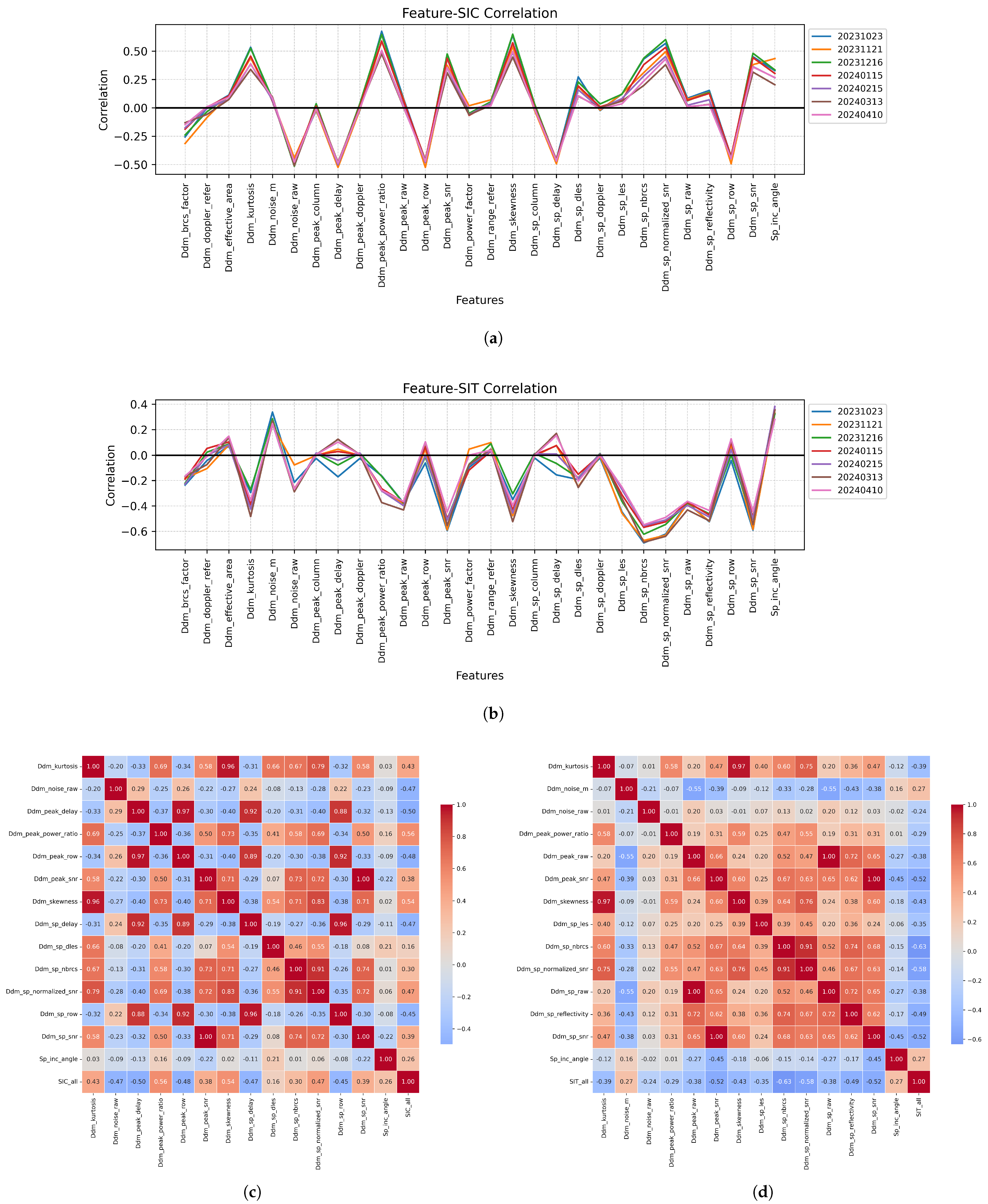
Excluding DDM raw counts and flag-type fields, there are a total of 28 feature parameters that can be used for sea ice retrieval, including parameters calculated by the DDM provided in the Tianmu-1 GNSS-R L1 data plus the incident angle at the specular point. Using all the features for SIC and SIT retrieval introduces redundancy and degrades accuracy; thus, we analyzed the correlation between each parameter and the SIC and SIT reference data. The correlation coefficients of all the features with the SIC and SIT are shown in Figure 2. The correlation coefficients were calculated for a randomly selected day each month from October 2023 to April 2024. The results were consistent across months. For SIC and SIT retrieval, 14 parameters from Tianmu-1 were selected for each, which are highly correlated with the respective reference data, as shown in Table 1.
Figure 2.
Feature correlation analysis: (a) Correlation between all features and SIC; (b) Correlation between all features and SIT; (c) Cross-correlation matrix of the 14 parameters for SIC retrieval; (d) Cross-correlation matrix of the 14 parameters for SIT retrieval.
The specific selection rationale is as follows. Nine parameters, including Ddm_kurtosis and Ddm_noise_raw, demonstrated high correlation coefficients with both SIC and SIT. Consequently, they were utilized in the retrieval models for both parameters. Another five parameters, such as Ddm_peak_delay and Ddm_peak_row, were highly correlated with SIC but showed low correlation with SIT. Thus, they were employed exclusively for SIC retrieval. Conversely, five other parameters, including Ddm_noise_m and Ddm_peak_raw, exhibited high correlation with SIT but low correlation with SIC, leading to their exclusive use in SIT retrieval. Furthermore, features like Ddm_peak_column, Ddm_power_factor, and Ddm_sp_doppler showed correlation coefficients close to zero with both SIC and SIT. These low-correlation parameters were consequently excluded from our models and were not used in the retrieval of either concentration or thickness.
The descriptions of each parameter are as follows.
- Ddm_kurtosis: Kurtosis of raw counts in the whole DDM;
- Ddm_noise_m: The ratio of the square of the mean of the noise floor and the variance of the noise floor;
- Ddm_noise_raw: The mean noise floor of the raw DDM;
- Ddm_peak_delay: Delay of the DDM peak bin, in corresponding GNSS system chip;
- Ddm_peak_power_ratio: Sum of centered 5 × 3 DDM power bin values around the specular point divided by the sum of the all DDM power bin values;
- Ddm_peak_raw: Peak value in DDM raw counts;
- Ddm_peak_row: The zero-based delay row of the peak value in the DDM;
- Ddm_peak_snr:, where is the maximum value (in raw counts) in a single DDM bin and is the the average per-bin raw noise counts;
- Ddm_skewness: Skewness of raw counts in the whole DDM;
- Ddm_sp_delay: Specular point delay in the DDM;
- Ddm_sp_dles: The slope of the second derivative of the DDM’s leading edge slope;
- Ddm_sp_les: Leading edge slope of a 3 delay × 5 Doppler bin box centered at the specular point bin;
- Ddm_sp_nbrcs: Normalized BRCS of a 3 delay × 5 Doppler bin box centered at the specular point bin;
- Ddm_sp_normalized_snr: SNR at specular point normalized by bistatic radar equation;
- Ddm_sp_raw: Value of the specular point in the DDM raw counts;
- Ddm_sp_reflectivity: Signal reflectivity at the specular point assuming coherent scattering;
- Ddm_sp_row: The zero-based delay row of the specular point delay in the DDM based on the specular point calculated on the ground;
- Ddm_sp_snr: , where is the value of specular point (in raw counts) in a single DDM bin and is the the average per-bin raw noise counts;
- Sp_inc_angle: The specular point incidence angle. This is the angle between the line normal to the Earth’s surface at the specular point and the line extending from the specular point to the spacecraft.
3.2. Retrieval Model
This study employed Extreme Gradient Boosting (XGBoost), an efficient machine learning algorithm based on gradient-boosted decision trees, proposed by Chen and Guestrin [37]. XGBoost fits additive regression trees iteratively to the residuals, improving the retrieval accuracy at each step. Compared with traditional gradient boosting, XGBoost incorporates enhancements in objective function optimization, regularization, parallel computation, and engineering efficiency.
Let the training set be , where are the feature vectors and are the target values. The XGBoost model approximates the target function using K regression trees:
where denotes the space of the regression trees.
At iteration t, the model learns a new tree by minimizing the regularized objective function:
where is the loss function, and the regularization term is
which penalizes tree complexity (here, T is the number of leaves and is the leaf weight).
By applying a second-order Taylor expansion to the loss function around , and defining the first and second derivatives as and , respectively, the optimal leaf weight and split decisions are obtained via a greedy algorithm to maximize the reduction in the objective value.
The algorithmic innovation of XGBoost lies in its scalable tree boosting architecture, which incorporates key advancements such as a regularized learning objective to mitigate overfitting, an efficient handling of sparse data, and a weighted quantile sketch for approximate tree learning. These features collectively enhance computational efficiency and predictive accuracy. Building upon this robust framework, this study focuses on its application for the retrieval of sea ice parameters.
The dataset was randomly split into training and validation sets at a ratio of 8:2 and constructed the test set by randomly selecting one day per month. To maximize model performance, a comprehensive hyperparameter tuning process was conducted. Based on the predefined search ranges presented in Table 2, an initial grid search with 5-fold cross-validation was performed to identify promising regions in the hyperparameter space. This was followed by a controlled variable method to fine-tune each parameter sequentially within those regions. The final settings are as follows: max_depth = 10, learning_rate = 0.1, n_estimators = 1500, reg_alpha = 1, and reg_lambda = 2.0. This combination was further validated using a random search, which consistently yielded optimal parameters within the vicinity of the grid search results, confirming the robustness of our selected hyperparameters.
Table 2.
XGBoost hyperparameters grid search range.
During the experiment, two comparison models were selected: a random forest model with a tree-based stacking structure similar to XGBoost and a neural network model with a completely different structure. The RF is an ensemble method that builds multiple decision trees using different bootstrap samples and feature subsets and average their predictions to reduce variance and improve accuracy [38]. RF has been successfully applied to GNSS-R SIT retrieval, achieving RMSE values of 0.032 m (GPS) and 0.036 m (BDS), as reported by Li et al. [22]. NNs consist of interconnected layers of neurons with trainable weights and activation functions. Their effectiveness has been demonstrated in sea ice detection [10], SIC retrieval [10,13], and SIT retrieval [20].
The same data were used to construct different models to confirm the reliability of the XGBoost retrieval model. The mapping relationship between the input and output can be expressed as follows:
where Y denotes the target SIC or SIT, is the chosen retrieval model, and is the vector of DDM-based features. For SIC retrieval, comprises the 14 selected parameters; for SIT retrieval, we additionally incorporate auxiliary parameters, as discussed in Section 4.
3.3. Model Evaluation
Retrieval performance in this study was evaluated using the correlation coefficient (R), mean absolute error (MAE), and root mean squared error (RMSE):
Here, is the model-estimated SIC or SIT, is the corresponding reference value, n is the sample size, and and denote the mean values of the reference data and model estimates, respectively.
4. Results
We selected all the dates between 18 October 2023 and 12 April 2024, for the experiments because of the coverage range of the CS2SMOS SIT reference data. Approximately three days were selected each month, namely, one day at the beginning, middle, and end of each month, for a total of 20 days of data used for training.
As described in Section 3.2, the training set and validation set used for hyperparameter tuning were randomly split from data collected on these 20 days, meaning that their data distributions were similar. Thus, the results of the validation set may not accurately reflect the model’s performance on other data. Therefore, after model training, we added additional data from different dates as a test set to more robustly evaluate the retrieval performance. In this study, in addition to the results of the test set, it is also necessary to consider the performance of the model on all the dates. The test set was randomly selected on a day close to the middle of each month from November to March to preliminarily evaluate the overall retrieval performance for each month. When a model performed well on both the training set and the test set, it was used for daily retrieval of the SIC and SIT for all dates except the training set.
Unlike previous studies that used the TDS-1 satellite data [4], which received signals only from GPS, or the FY3E [18,22], which received reflected signals from both GPS and BDS, the Tianmu-1 satellite data used in this study simultaneously received reflections from four navigation systems: GPS, BDS, GAL, and GLO. Therefore, the retrieval models were constructed separately for each of these four signal sources, and the retrievals were performed independently.
4.1. Comparison of Different Algorithms
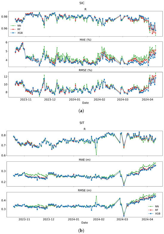
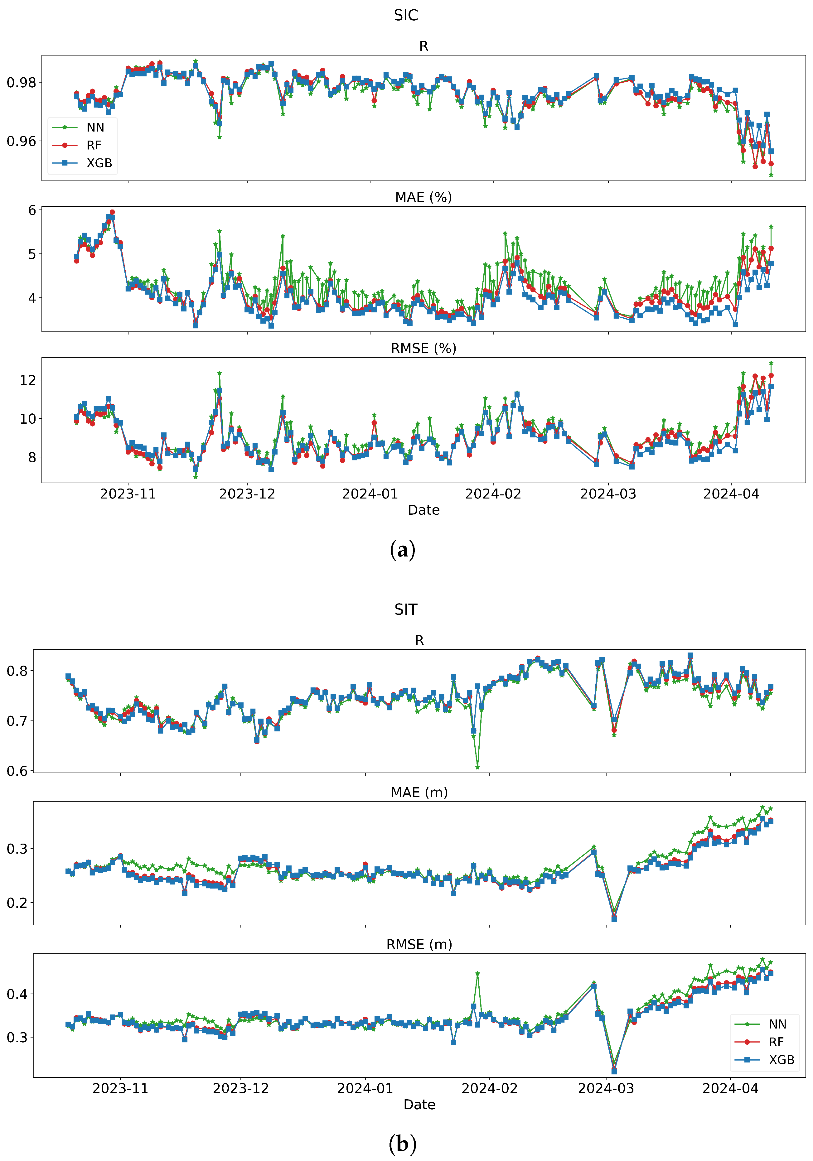
Using identical training and test datasets, we trained retrieval models for SIC and SIT data using XGBoost, RF and NN, respectively. The SIC and SIT retrieval models use the Tianmu-1 feature parameters selected in Table 1 as inputs, and the test set results of the different algorithms are summarized in Table 3. The daily evaluation metrics for the entire season are illustrated in Figure 3.
Table 3.
Performance comparison of different methods for retrievals on the test set.
Figure 3.
Temporal evolution of daily retrieval performance for the three machine learning models: (a) Sea ice concentration (SIC) and (b) Sea ice thickness (SIT). Colors represent different models: XGBoost (blue), Random Forest (red), and Neural Network (green). Metrics shown include correlation coefficient (R), mean absolute error (MAE), and root mean square error (RMSE) from October 2023 to April 2024.
With respect to the SIC and SIT retrievals, the three models performed similarly well. As shown in Table 3, on the test set, the XGBoost method performed better, with higher R values and lower MAEs and RMSEs. The daily retrieval results of the three methods are shown in Figure 3. On most dates, the blue dots representing the XGBoost model also had lower errors than the other two models did. Furthermore, in terms of computational speed and efficiency, XGBoost performed better overall. During the experimental process, significant differences in training time were observed among the three methods. The XGBoost model training was completed in less than 10 s, while RF required 10 min and 10 s, and NN took 26 min and 20 s (configured with 100 epochs and early stopping after 30 epochs without improvement). It should be noted that these time measurements represent the training duration for a single model only, excluding data processing, hyperparameter tuning, and prediction phases. In this study, we needed to train and evaluate 4 models for SIC retrieval and 16 models for SIT retrieval. Considering both computational speed and efficiency comprehensively, XGBoost exhibited clear advantages. Therefore, XGBoost was selected for subsequent retrieval studies.
4.2. SIC Retrieval Results
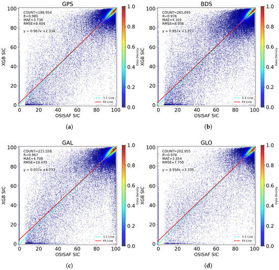
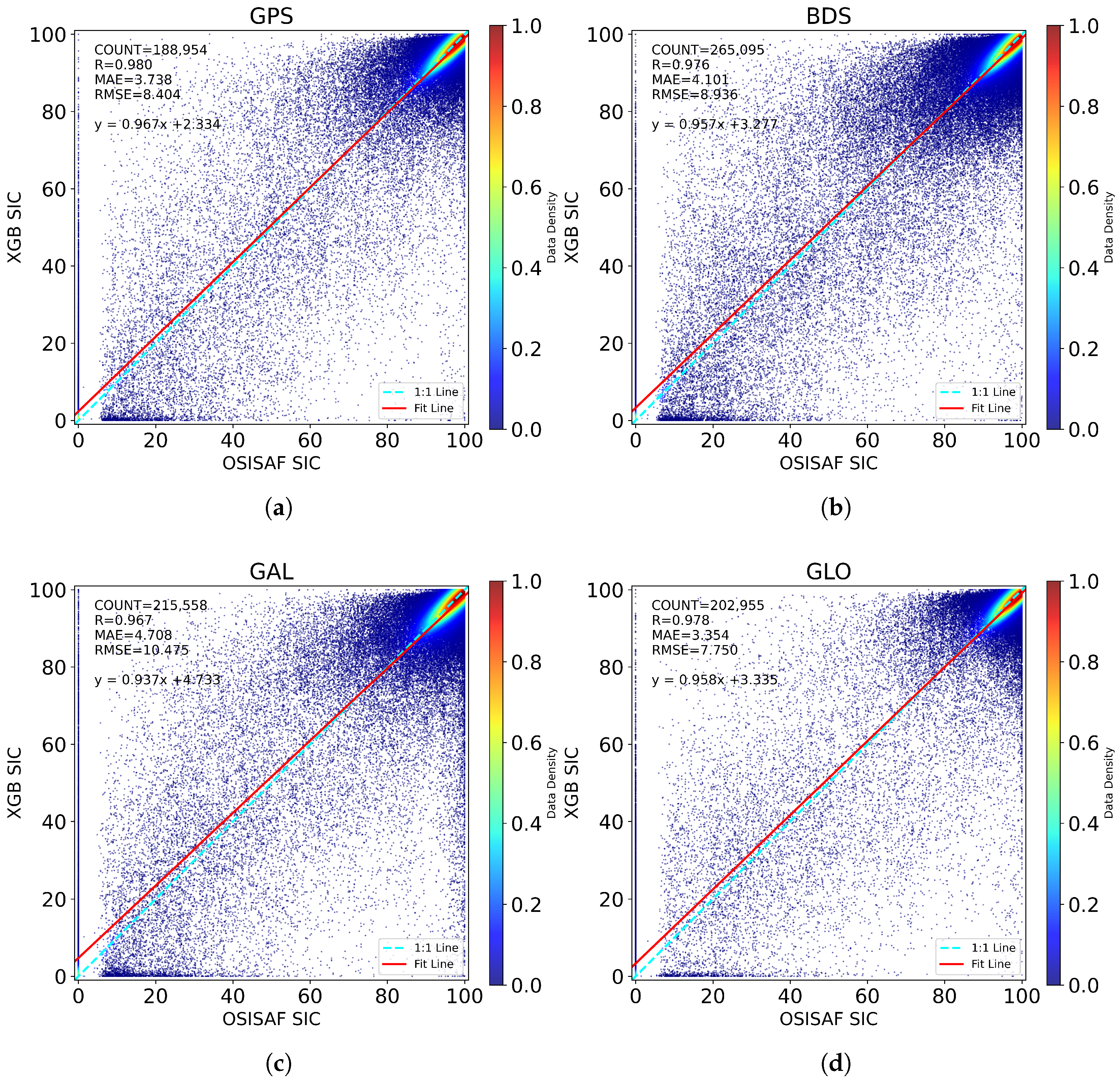
On the basis of the XGBoost algorithm model, 14 Tianmu-1 DDM parameters were used as inputs, and OSISAF SIC data were used as the output reference values. Four SIC retrieval models were trained and tuned separately for the four different GNSS data sources. The retrieval results on the test set are shown in Figure 4 and Table 4. As shown in Figure 4, during the Arctic winter, the SICs are mostly above 80%, and the retrieval results within the 80–100% range closely fit the 1:1 line with the reference data.
Figure 4.
Comparison between XGBoost-predicted SIC and OSISAF SIC for: (a) GPS, (b) BDS, (c) GAL, and (d) GLO. SIC_OSISAF is the SIC reference value, SIC_XGB is the estimated SIC from XGBoost model.
Table 4.
SIC retrieval performance using the 14 Tianmu-1 parameters across different GNSS systems.
Among the four GNSS sources, the retrieval performance was best for GLO and GPS. The GLO system achieved an RMSE of only 7.750% and an MAE of 3.354%, whereas GPS had RMSE and MAE values of 8.404% and 3.738%, respectively. However, compared with that for the GLO (R = 0.978), GPS yielded a higher correlation coefficient (R = 0.980). The performance of the BDS was slightly worse, and the performance of the GAL system was the poorest, with the RMSE exceeding 10%, the MAE exceeding 4.7%, and R = 0.967. Despite GAL having the worst test results compared with those of the GPS, the BDS, and GLO, overall, the SIC retrieval results for the Tianmu-1 data were satisfactory.
4.3. SIT Retrieval Results
With the use of the XGBoost model with 14 Tianmu-1 parameters, the SIT retrieval results are summarized in Table 5. SIT retrieval accuracy using only Tianmu-1 parameters is not as good as that for SIC. In the test set, the SIT retrieval performance of the BDS was the best, with correlation coefficients of 0.801 and MAE and RMSE values of 0.249 m and 0.334 m, respectively. GPS performed slightly worse, with an MAE of 0.250 m and an RMSE of 0.335 m, which were only 0.001 m different from those of the BDS. GAL was intermediate, whereas GLO performed the worst, with R = 0.734 and MAE and RMSE values of 0.287 m and 0.373 m, respectively.
Table 5.
SIT retrieval performance using only the 14 Tianmu-1 parameters across different GNSS systems.
Considering the limited accuracy of SIT retrieval with only Tianmu-1 parameters, we attempted to improve SIT estimation by including the following auxiliary parameters: SIC, sea ice salinity (S), and sea ice temperature (T). The SIC data were sourced from OSISAF, whereas the S and T data were derived from SMOS products [30]. We trained the models using four different input combinations and compared their performance on the same test set:
- 14 inputs: Tianmu-1 14 parameters only;
- 15 inputs: Tianmu-1 14 parameters + OSISAF SIC;
- 16 inputs: Tianmu-1 14 parameters + SMOS S and T;
- 17 inputs: Tianmu-1 14 parameters + SIC + S and T.
Since the S and T data were extracted from the same source, they were considered a joint input group. The retrieval results are shown in Table 6. Compared with that using the Tianmu-1 parameters alone, the inclusion of SIC improved the SIT retrieval accuracy; adding S and T data further enhanced the performance and yield better performance than that with the SIC-only input. Finally, the combination of SIC, S, and T slightly improved the results beyond those of S and T alone, demonstrating the positive contribution of all three auxiliary inputs across all four GNSSs.
Table 6.
Comparison of SIT retrieval performance with different input parameter combinations across 4 systems. The bold shows the performance is the best.
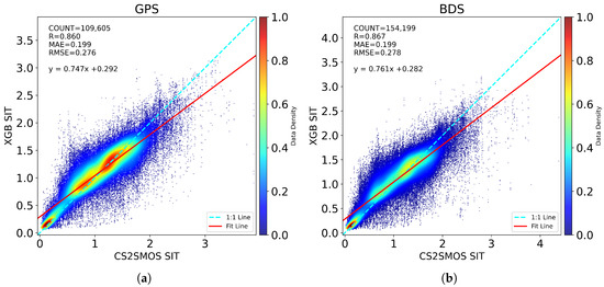
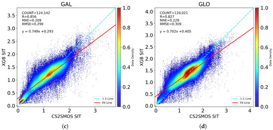
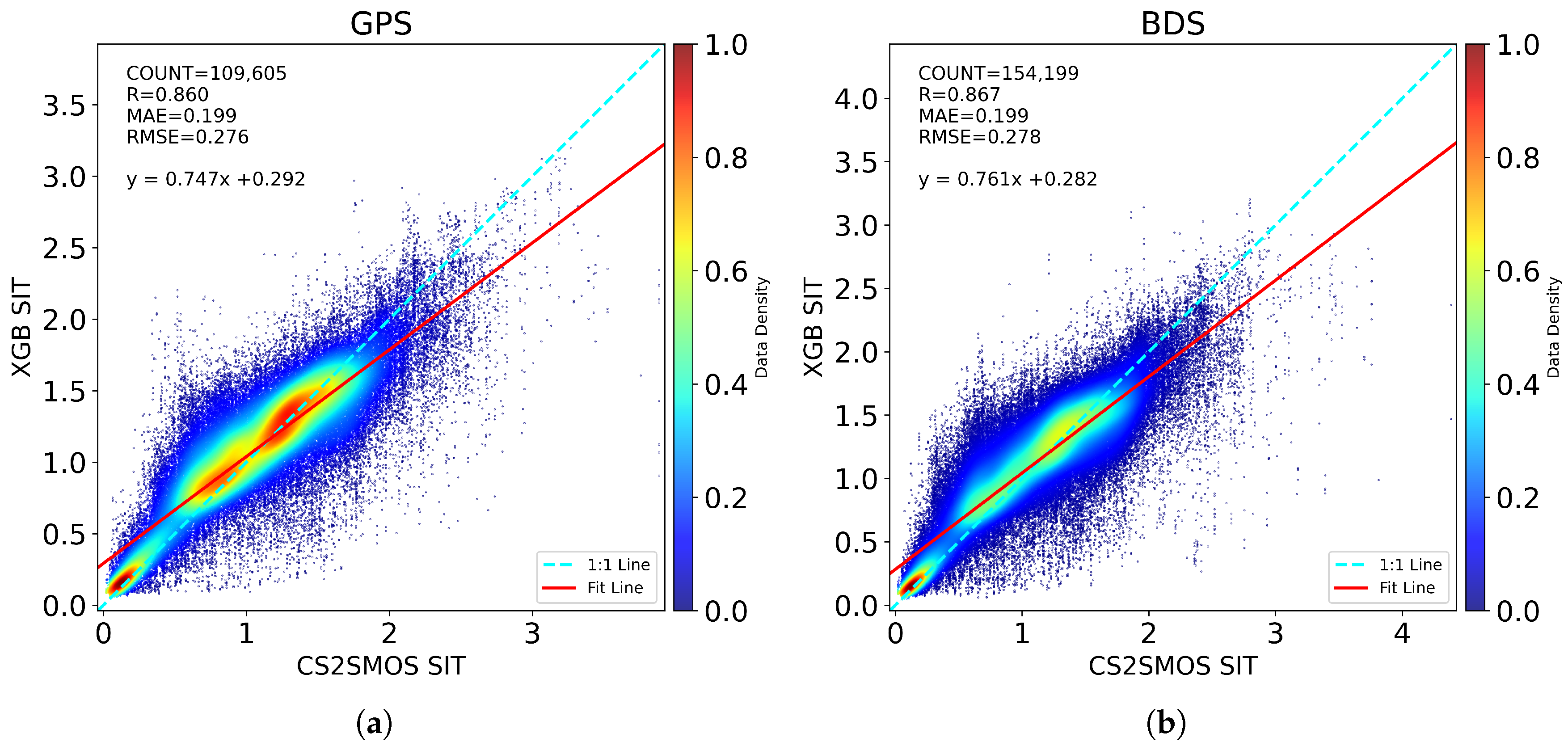
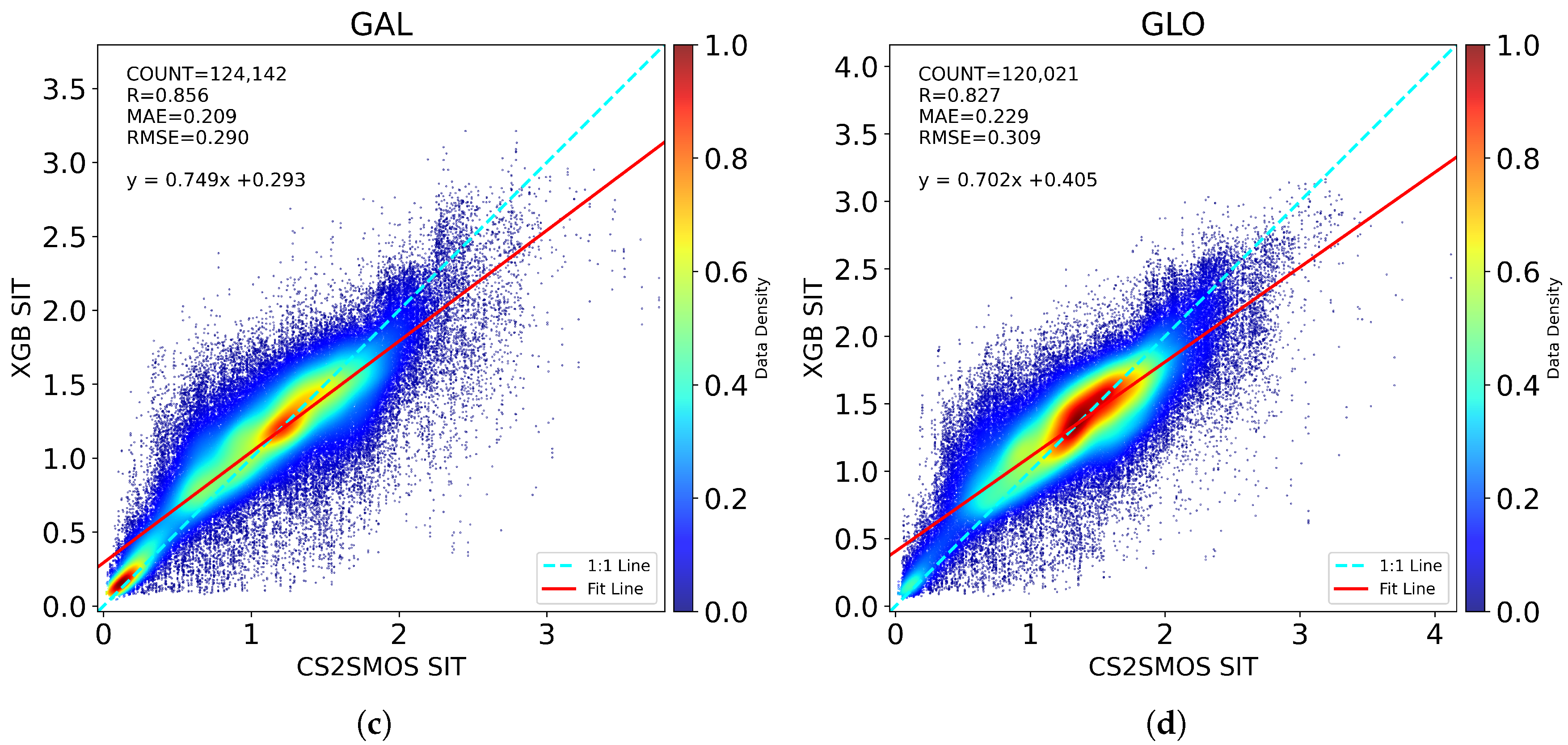
The distributions of the SIT retrieval results for GPS, BDS, GAL, and GLO on the test set compared with the reference values are shown in Figure 5. The SIT retrieval model used a 17-parameter combination (14 Tianmu-1 parameters + SIC + S, T), with the best results in Table 6 as input.
Figure 5.
Comparison between XGBoost-predicted SIT using 17 parameters and CS2SMOS SIT for: (a) GPS, (b) BDS, (c) GAL, (d) GLO. SIT_CS2SMOS is the SIT reference value, SIT_XGB is the estimated SIT from XGBoost model.
4.4. Daily Retrieval
To validate the applicability of the retrieval models, all data from the entire season (excluding training dates) were processed and filtered identically. The trained models were then applied to retrieve the SIC and SIT daily, and the retrieval results were evaluated with reference data using the R, MAE, and RMSE metrics.
4.4.1. Daily SIC Retrieval
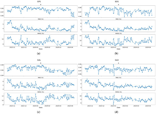
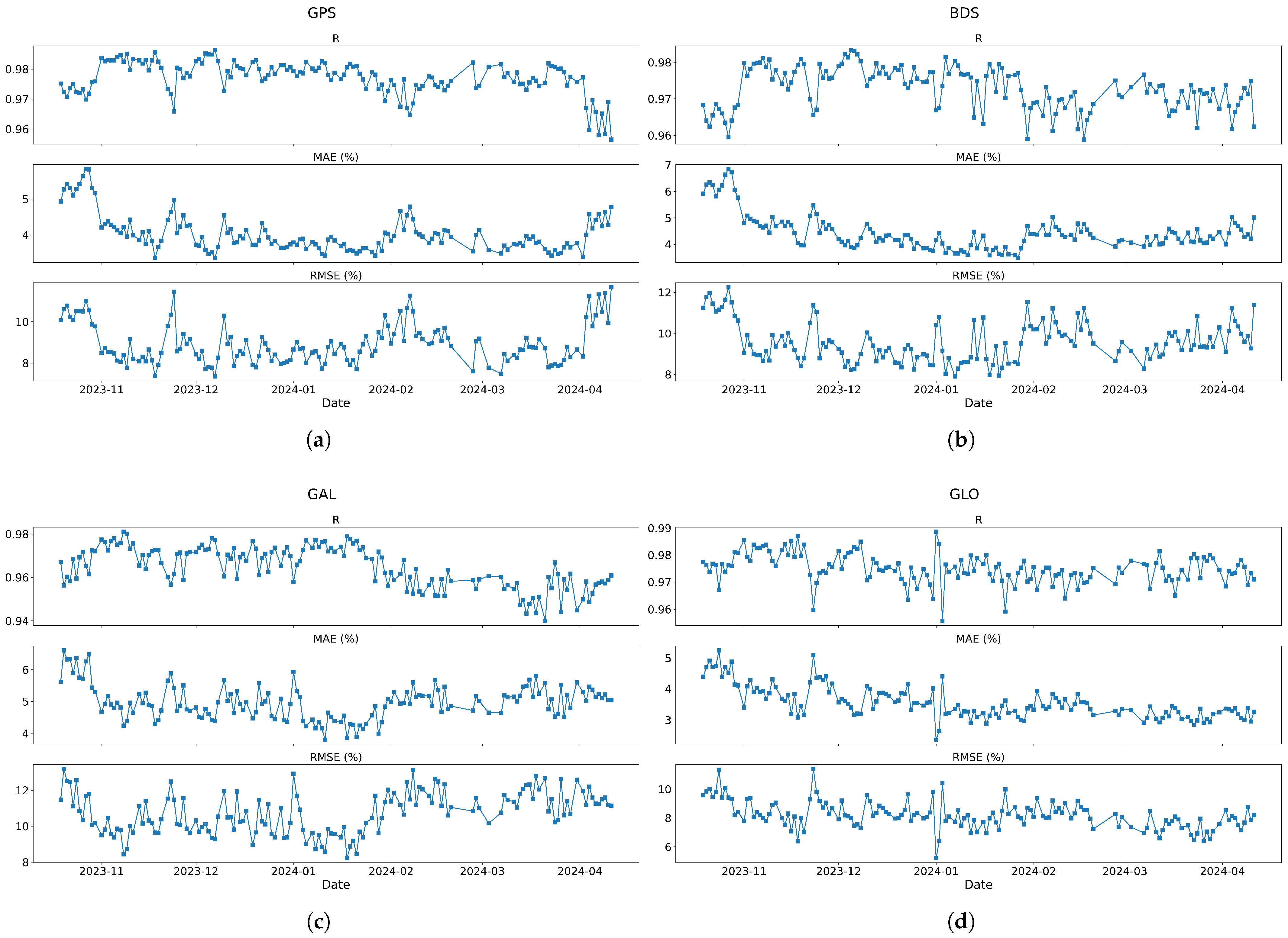
As shown in Figure 6, R generally remained above 0.95 across all the dates. Only on a few GAL dates did R decrease to approximately 0.94. Otherwise, very high correlations were observed. With respect to the MAEs, the GPS and BDS results were mostly between 3% and 7%, mostly near 4%. The MAEs for GAL ranged from 4% to 7%, mostly near 5%. The MAEs for GLO ranged from 2% to 5% and were near 3.5% for most dates. The RMSE values for all four systems were generally between 6% and 13%. Except for that of GAL, which occasionally exceeded 10%, the RMSE values of the other three GNSSs mostly remained below 10%.
Figure 6.
Daily SIC retrieval performance trends for: (a) GPS, (b) BDS, (c) GAL, and (d) GLO. Each panel shows R, MAE, and RMSE trends from October 2023 to April 2024.
Table 7 shows that the daily average performance of the four GNSSs is consistent with the test set results shown in Table 4, confirming the stability of the model in random test sets and full seasonal data.
Table 7.
Statistical summary of daily SIC retrieval performance (mean ± standard deviation) across GNSS systems.
4.4.2. Daily SIT Retrieval
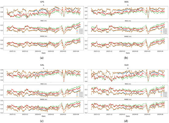
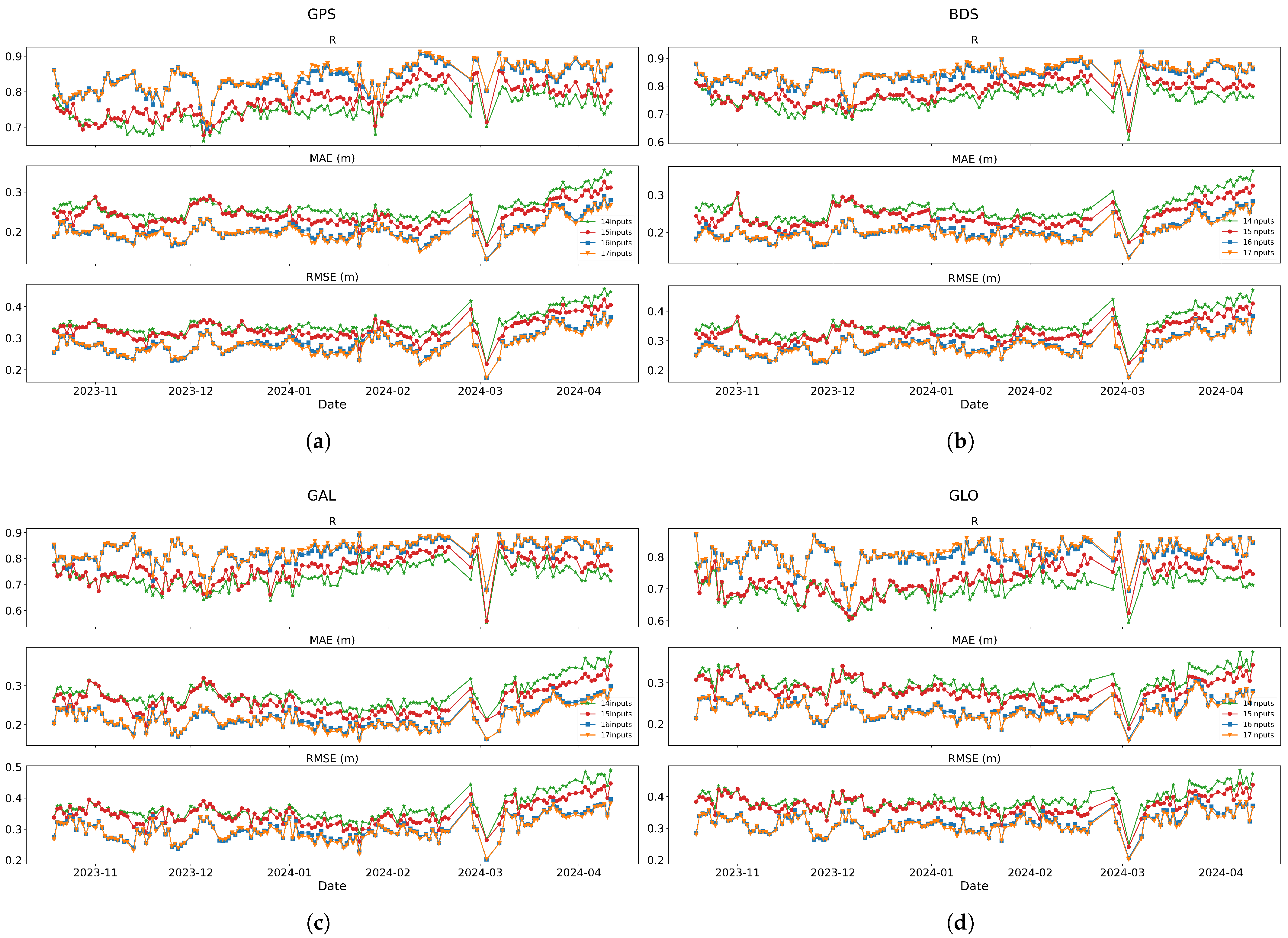
The data for all the dates were processed in the same way, and SIT daily retrieval was subsequently performed to obtain the R, MAE, and RMSE trends for each day’s retrieval results, as shown in Figure 7 and Table 8. The green points correspond to Tianmu-1 14 parameters only, consistently showing the lowest R and highest errors, indicating the weakest correlation and largest retrieval errors. When SIC, S, and T were added as auxiliary inputs, R increased, whereas the MAE and RMSE decreased, indicating improved accuracy.
Figure 7.
Daily SIT retrieval performance with different input parameter combinations for: (a) GPS, (b) BDS, (c) GAL, and (d) GLO. Each panel shows R, MAE, and RMSE trends from October 2023 to April 2024. Green: Tianmu-1 14; Red: Tianmu-1 14 + SIC; Blue: Tianmu-1 14 + S, T; Orange: Tianmu-1 14 + SIC + S, T.
Table 8.
Statistical summary of daily SIT retrieval performance (mean ± standard deviation) using optimal parameter combinations across GNSS systems.
The different performance of GNSS constellations in SIC and SIT retrievals is notable. In particular, the GLO signals yield the best performance for SIC retrieval but the weakest performance for SIT retrieval. This contrast can be explained by the different physical sensitivities of the two retrieval targets. SIC retrieval primarily relies on the DDM waveform, which are closely related to surface roughness. Among the four GNSS systems, GLO has the largest waveform coverage area, resulting in superior SIC retrieval performance. In contrast, SIT retrieval is more strongly controlled by the surface reflectivity. The GLO exhibits the lowest calibration accuracy among the four GNSS systems [24], which degrades the reliability of reflectivity-based thickness estimation and results in poorer SIT retrieval performance.
Overall, these results confirmed the feasibility of using Tianmu-1 GNSS-R data for both SIC and SIT retrievals. They also demonstrated that for all dates in the Arctic winter, the daily retrieval results of this method were within a relatively stable range. Furthermore, regardless of the retrieval algorithm used, the results for all the dates exhibited the same temporal variation trends. On the data showing pronounced fluctuations, similar deviations occurred across all the algorithms, indicating that such anomalies were driven by the characteristics or quality of the input data rather than by the retrieval model itself. This suggests that occasional data quality issues may introduce significant local biases, affecting the overall accuracy. Daily retrieval results from Figure 6 and Figure 7 reveal pronounced seasonal variations in inversion errors, with significant increases observed in October and April. These two periods correspond respectively to the onset of the ice-covered season and the early stages of the melting season. During these transitional phases, the surface conditions are more complex due to the coexistence of open water, newly formed ice, melting ice, and variable surface roughness. Such complexity reduces the robustness of SIC and SIT retrievals based on surface reflection characteristics, leading to larger errors compared to the more stable mid-winter ice-covered period.
5. Discussion
5.1. Analysis by Distribution
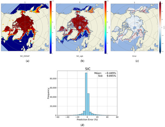
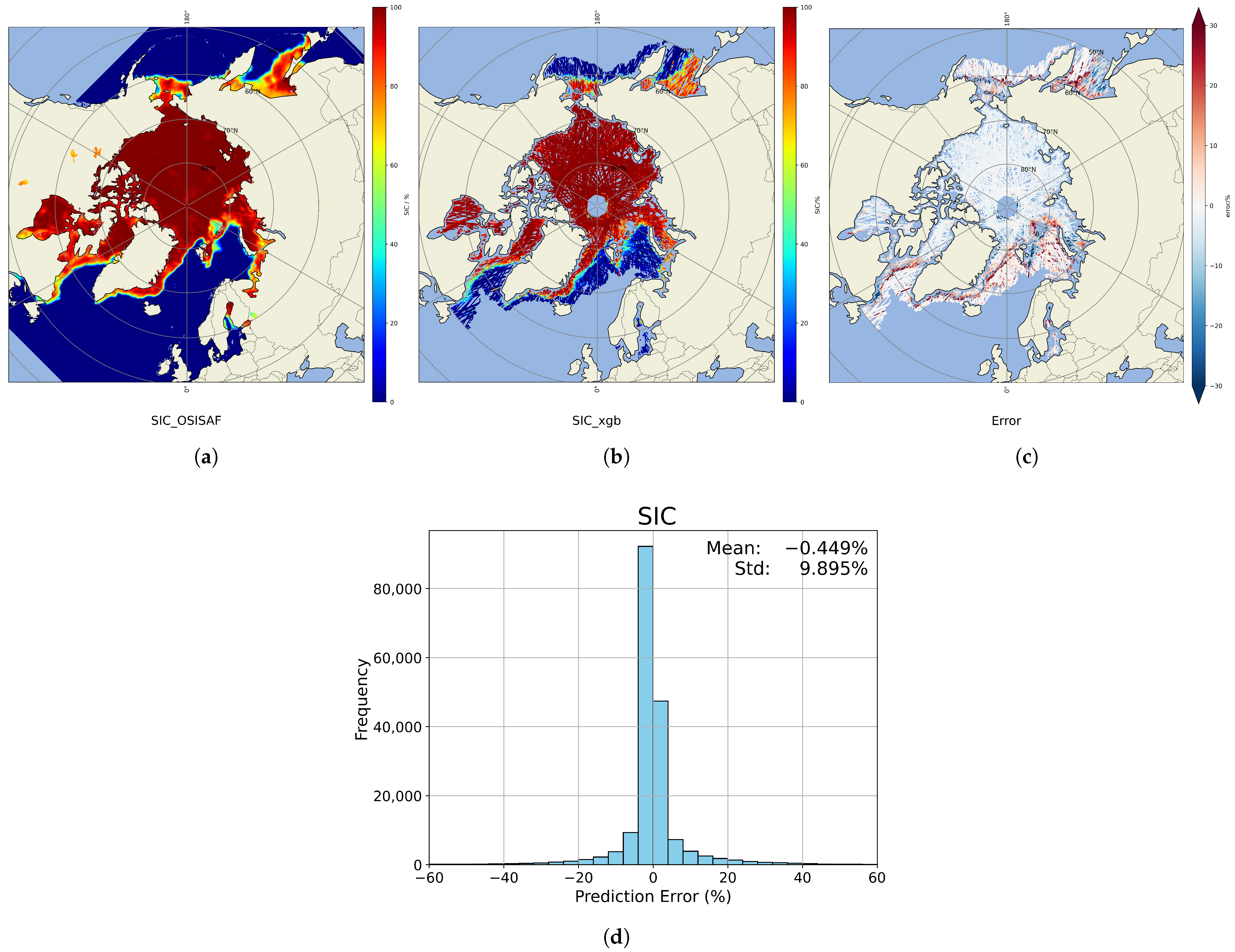
Figure 8 presents the projected distributions and error histograms of the SIC retrieval results obtained on 9 February 2024. For these plots, the data from the four types of GNSSs were processed separately using their corresponding models, and the final aggregated SIC field was obtained by combining all the results.
Figure 8.
SIC retrieval results for 9 February 2024. (a) OSISAF reference SIC field. (b) The model-predicted SIC. (c) Prediction error map (predicted minus reference). (d) Histogram of SIC prediction errors obtained on 9 February 2024, calculated as the difference between model-predicted and OSISAF reference SIC values (units: %).
Figure 8 shows that most retrieval errors on this date were concentrated within ±25%. Figure 8b reveals that the SIC distribution retrieved using the XGBoost model closely matched the OSISAF reference data in the high-concentration ice regions of the Arctic, where errors were near zero. In contrast, in marginal ice zones, particularly in mixed ice–water regions, the retrieval exhibited larger errors, with absolute values exceeding 20% in some cases. On 9 February 2024, a total of 181,028 SIC samples were available. As shown in Figure 8d, approximately 130,000 samples had an error close to zero, accounting for more than two-thirds of the total samples. Among the remaining less than 50,000 samples, only a very small proportion had an error exceeding ±30%.
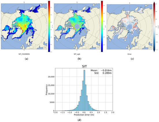
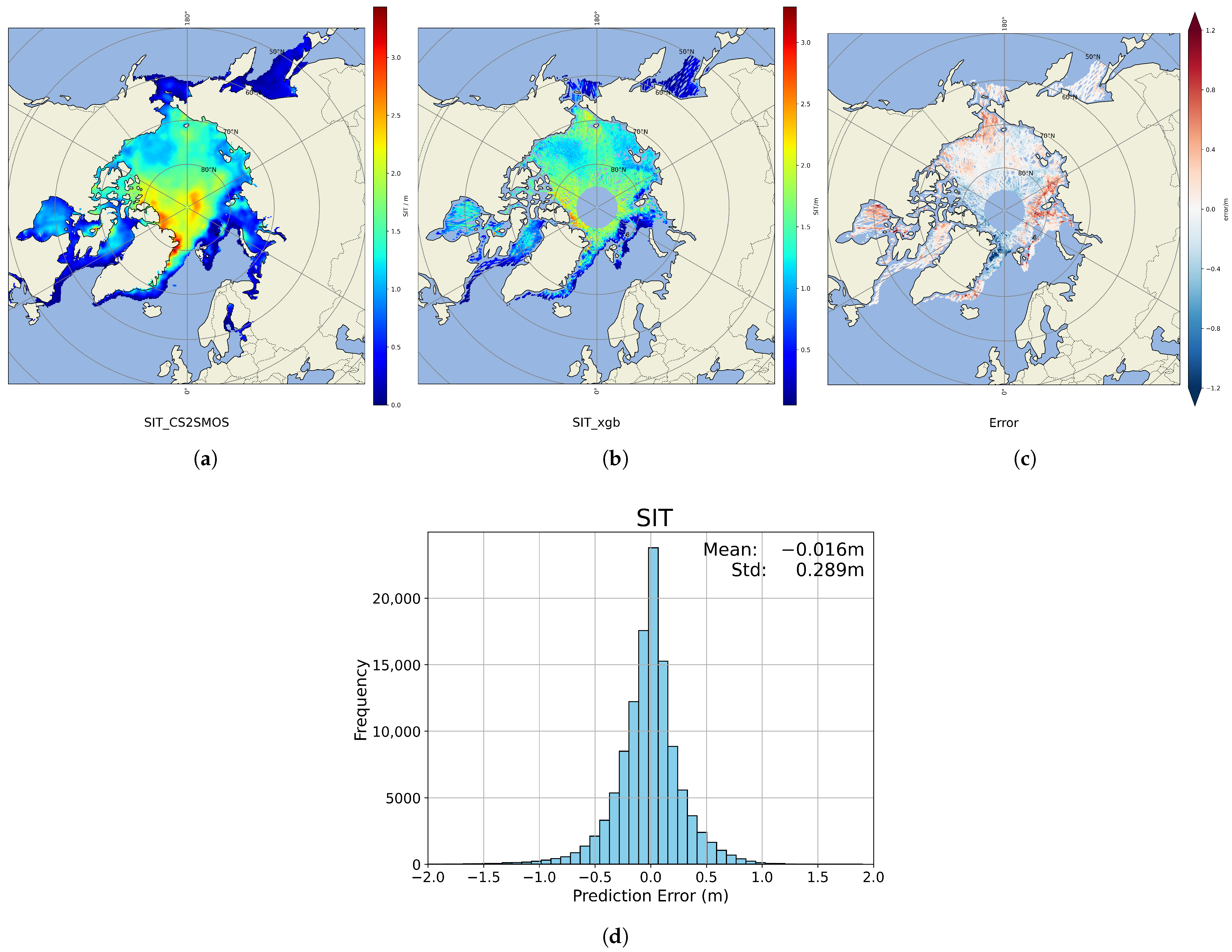
The SIT retrieval results and corresponding error distribution for the same date are shown in Figure 9, which is based on a total of 117,299 samples from all four GNSS constellations. Most SIT retrieval errors fell within ±1 m. The spatial comparison in Figure 9b reveals that retrievals were more accurate in thin-ice concentration zones, whereas larger discrepancies occurred near coastlines and in thick-ice areas exceeding 3 m. As shown in Figure 9d, more than 90,000 samples had errors within ±0.5 m, while fewer than 30,000 samples (less than one-quarter of the total samples) had larger errors.
Figure 9.
SIT retrieval results for 9 February 2024. (a) CS2SMOS reference SIT field, (b) The model-predicted SIT. (c) Prediction error map (predicted minus reference). (d) Histogram of SIT prediction errors, calculated as the difference between model-predicted and CS2SMOS reference SIT values (units: m).
After the retrieved SIC and SIT results were projected onto the Arctic region map, they maintained a distribution similar to that of the reference data. The larger retrieval errors observed in marginal ice zones and coastal regions for both SIC and SIT can be attributed to the increased complexity of surface conditions in these areas. Marginal ice zones are typically characterized by mixed ice–water coverage, newly formed or melting ice, and strong spatial and temporal variability driven by sea ice dynamics. Coastal regions are further influenced by land contamination and rapidly changing ice conditions. Since the GNSS-R-based retrieval approach primarily relies on information derived from reflected signals, such heterogeneous and dynamic surface conditions can reduce the stability of the reflection characteristics and increase retrieval uncertainty. Consequently, larger errors are expected in these regions.
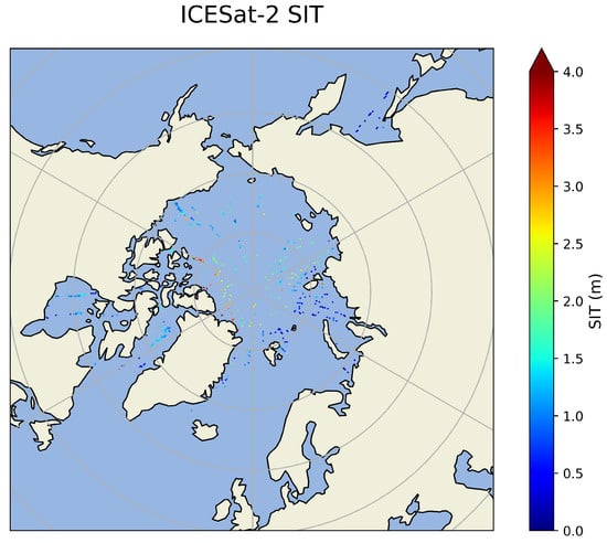
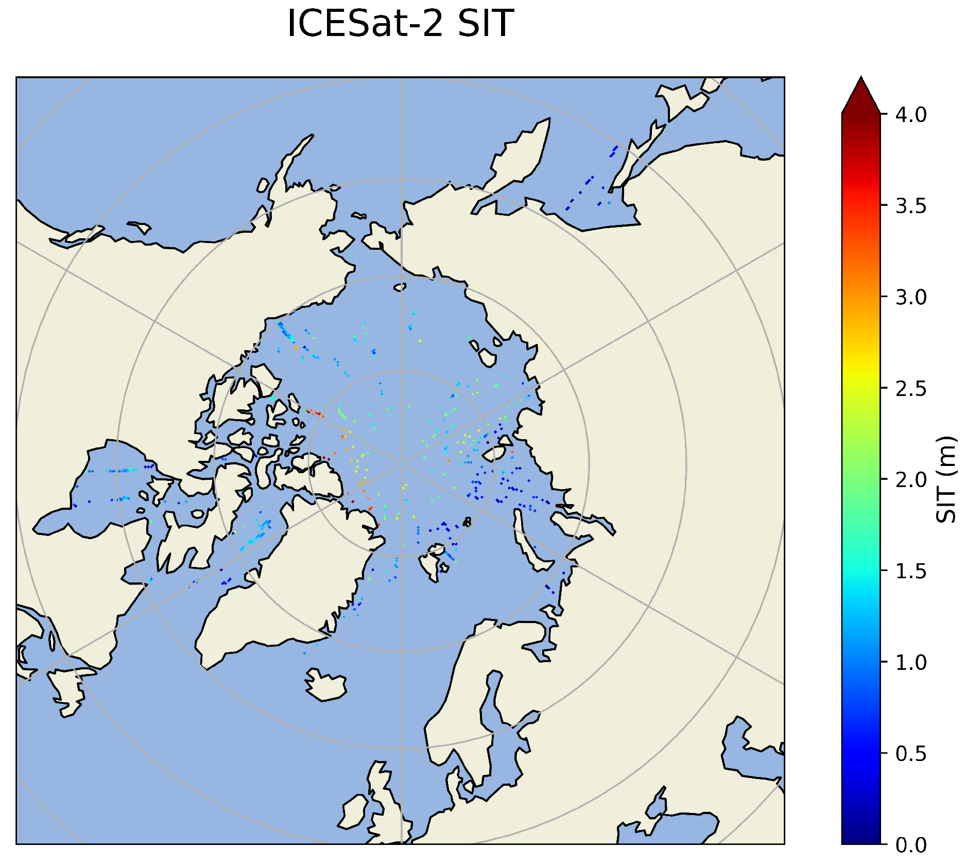
We use the monthly gridded winter Arctic sea ice thickness (SIT) product derived from ICESat-2 (IS2SITMOGR4, Version 3), distributed by the National Snow and Ice Data Center (NSIDC). This product provides Arctic-wide SIT estimates from November 2018 onward during the freezing season (September–April), gridded onto a 25 km × 25 km North Polar Stereographic grid. Sea ice thickness is estimated using ATLAS/ICESat-2 L3A Sea Ice Freeboard (ATL10) Version 6 data and NASA Eulerian Snow On Sea Ice Model (NESOSIM) snow loading. Ref. [39] Figure 10 shows the spatial distribution of ICESat-2 SIT observations on 9 February 2024. In contrast to the spatially continuous SIT field retrieved by our XGBoost-based model (Figure 9b), the IS2 SIT observations are notably sparse.
Figure 10.
Distribution of ICESat-2 SIT observations on 9 February 2024.
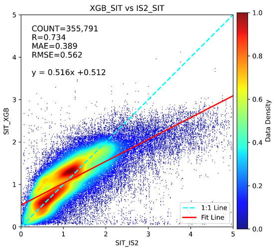
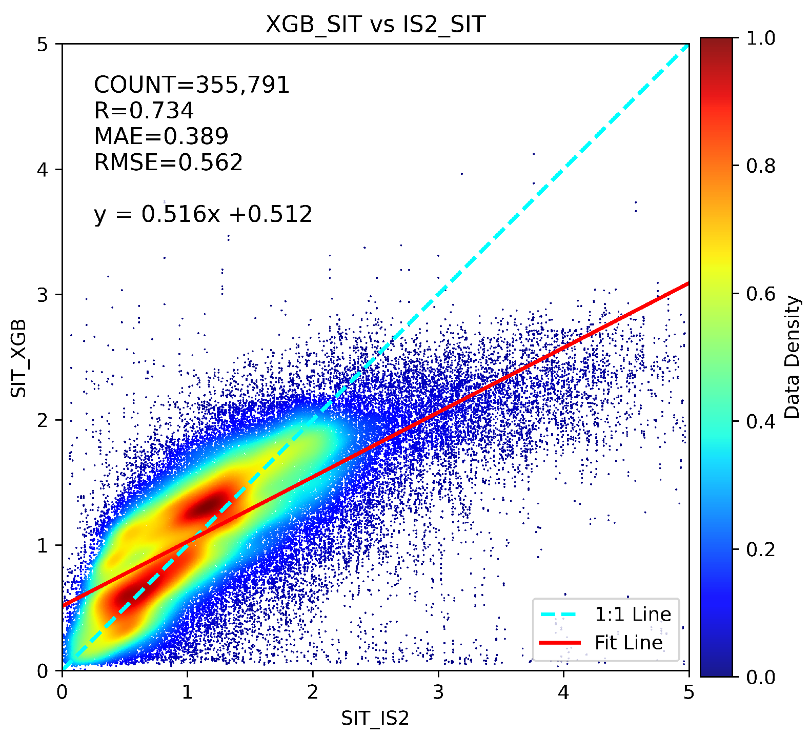
To quantitatively evaluate the SIT results in this study, we exclude all training dates and perform a spatiotemporal collocation between the daily XGBoost SIT and the IS2 SIT product for each remaining day. After matching, a total of 355,791 collocated data pairs are obtained. The comparison results are summarized in Figure 11. The overall correlation coefficient between the two datasets is R = 0.734, with the MAE of 0.389 m and the RMSE of 0.562 m. On the whole, the comparison indicates good agreement between the XGBoost-retrieved SIT and the IS2 SIT product, particularly within the 0–2 m thickness range, where most data points cluster closely around the 1:1 line. For thicker ice (>3 m) in the IS2 product, our retrievals tend to underestimate sea ice thickness.
Figure 11.
Comparison between XGBoost-predicted SIT and ICESat-2 SIT for all matched data points excluding the training period.
5.2. Analysis by Category
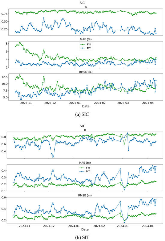
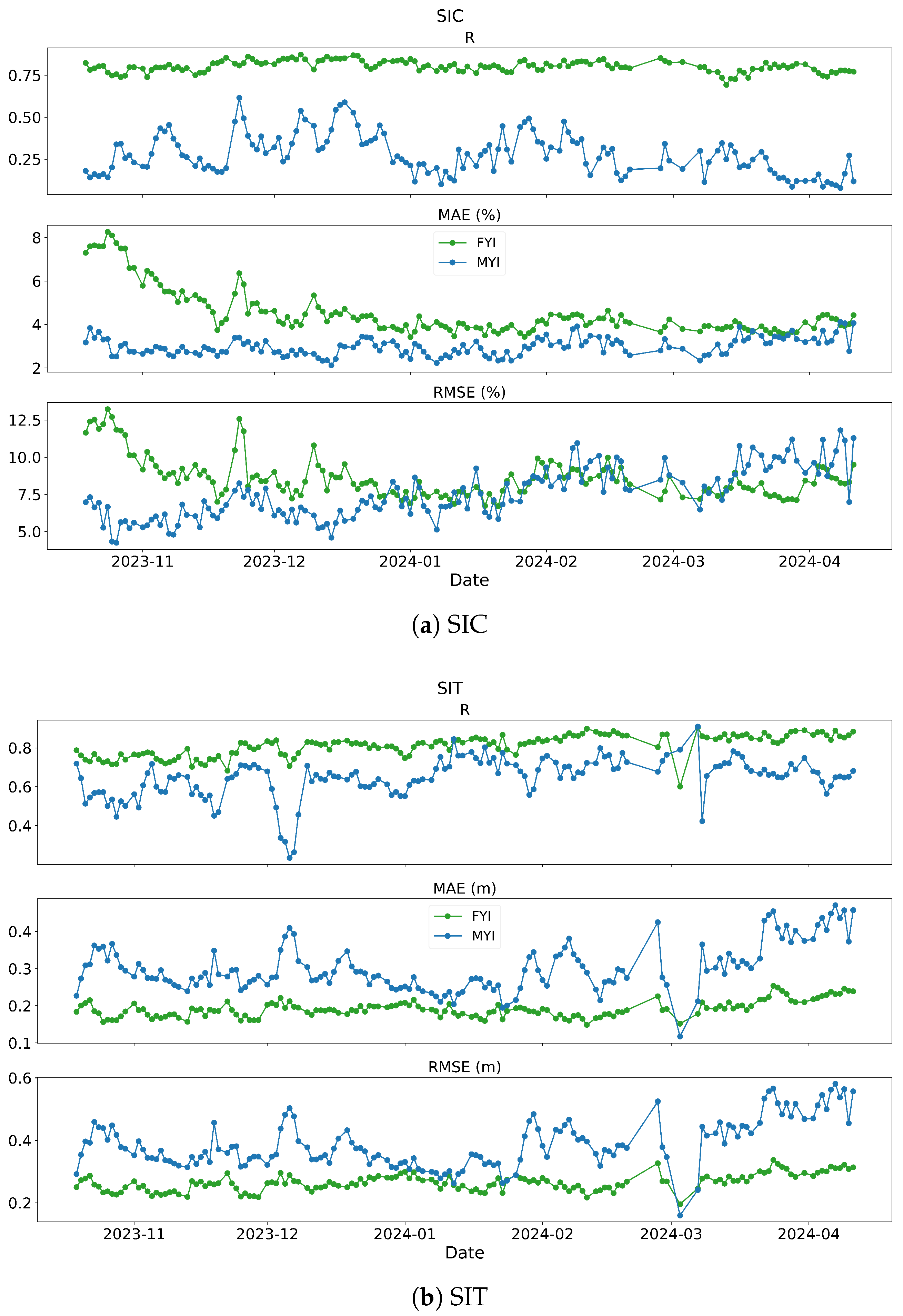
This study also evaluated the retrieval results for different sea ice types. The SIC and SIT retrievals from the four GNSS systems (GPS, BDS, GAL, GLO) presented in Section 5.1 were aggregated to obtain daily comprehensive retrieval results. The OSI SAF sea ice type data were spatiotemporally matched with our daily retrieval results, enabling separate evaluation for first-year ice (FYI) and multi-year ice (MYI). As shown in Figure 12, the green points represent the R, MAE, and RMSE values comparing FYI retrieval results with reference data, while the blue points represent the corresponding metrics for MYI.
Figure 12.
Evaluation metrics for different sea ice types. (a) SIC retrieval performance for FYI (green) and MYI (blue); (b) SIT retrieval performance for FYI (green) and MYI (blue), showing R, MAE, and RMSE trends from October 2023 to April 2024.
For SIC retrieval, FYI exhibits consistently high and stable correlation coefficients (R) when compared with OSISAF SIC data, whereas MYI shows lower correlations with significant fluctuations throughout the seasonal cycle. This discrepancy arises because reference SIC values for MYI predominantly fall within a narrow range of 95–100%. When retrieval results deviate from this interval, it substantially reduces the correlation coefficient, leading to the observed high variability in MYI correlations. In contrast, FYI reference SIC values span a wider range, and the retrieval results generally fall within this reference interval, resulting in more stable overall correlation coefficients. Therefore, relying solely on correlation coefficients for retrieval evaluation is insufficient, and error metrics must be comprehensively considered. The MAE for MYI ranges between 2–10%, and RMSE varies from 4–14%, with error fluctuations generally within ±10%, indicating relatively stable error performance overall. During the initial freezing period from October to November 2023, FYI errors were generally larger. As the season progressed and sea ice conditions stabilized, FYI errors gradually decreased, approaching those of MYI, with FYI even exhibiting lower RMSE than MYI during certain periods. By March-April 2024, as partial sea ice began to melt and sea surface conditions became more complex, retrieval difficulty increased, and RMSE in MYI regions gradually rose.
For SIT retrieval, FYI generally demonstrates higher correlation coefficients and lower errors compared to CS2SMOS SITs. Throughout the freezing period series, the evaluation metrics (R, MAE, RMSE) for FYI show minimal dramatic fluctuations, maintaining overall stability. In contrast, MYI SIT retrievals perform consistently worse than FYI throughout the winter season, exhibiting lower correlations, larger errors, and greater variability in evaluation metrics. Particularly after mid-March 2024, MYI SIT errors increased significantly and exceeded those of FYI on the same dates, a pattern consistent with the trends observed in Figure 7. Therefore, the fluctuations in Arctic winter ice thickness retrieval errors are primarily attributable to MYI retrieval errors. Since MYI regions predominantly consist of thick ice while FYI regions mainly comprise thin ice, these findings align with the conclusion drawn in Section 5.1 that thin ice regions yield better retrieval performance than thick ice regions.
5.3. Feature Importance Analysis by SHAP
To further investigate the physical relevance of the input variables used in the SIC and SIT retrieval models, we apply SHapley Additive exPlanations (SHAP) to quantify the contribution of each feature to the XGBoost regression outputs. SHAP [40] is a game-theory-based interpretability framework that attributes the prediction of a machine-learning model to individual input features by computing Shapley values, which represent the average marginal contribution of a feature across all possible feature combinations. The mean absolute SHAP value of each feature therefore provides a global measure of its overall importance, indicating how strongly the feature influences the model output on average.
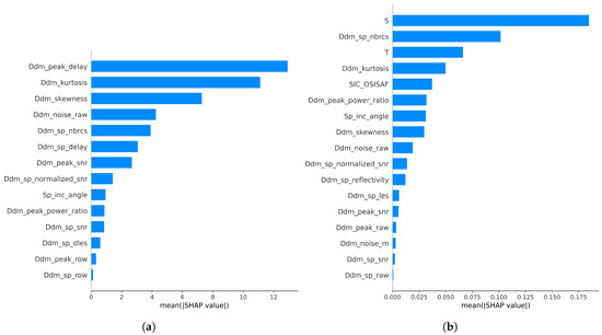
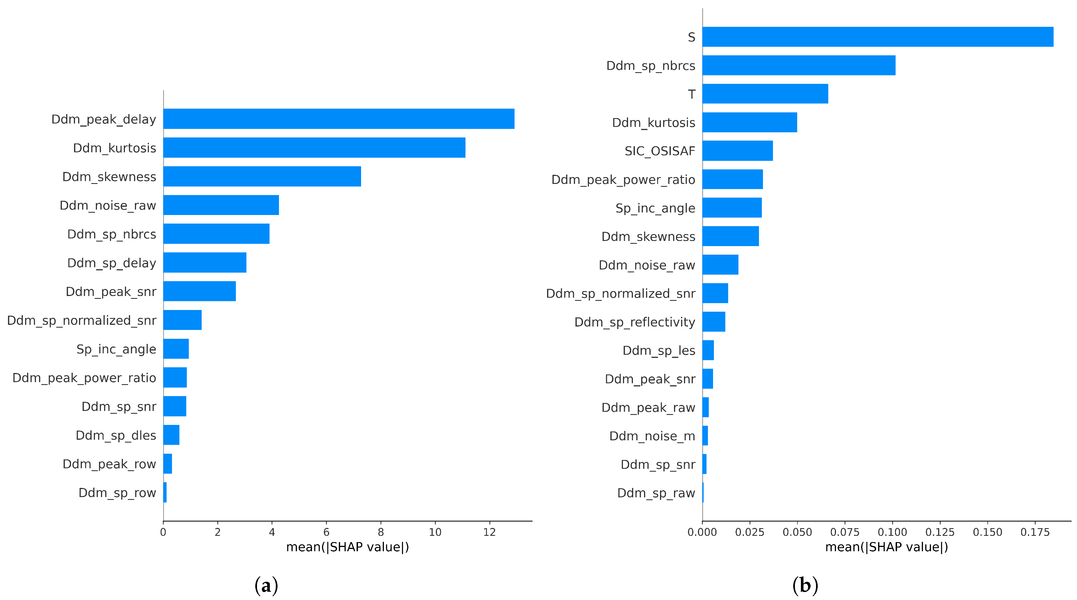
Figure 13 shows the feature importance rankings for the SIC and SIT retrieval models, respectively, based on the mean absolute SHAP values. Larger SHAP values indicate a stronger impact of the corresponding feature on the predicted variable. The physical description of these parameters is described in detail in Section 3.1.
Figure 13.
SHAP-based feature importance for the XGBoost models: (a) SIC retrieval and (b) SIT retrieval.
For the SIC retrieval model, the three most influential features are Ddm_peak_delay, Ddm_kurtosis, and Ddm_skewness (Figure 13a). These three parameters are directly related to variations of DDM power along the delay dimension and therefore reflect the degree of waveform spreading in the DDM. The extent of DDM spreading is strongly controlled by the roughness of the reflecting surface. Different sea ice concentration conditions correspond to different proportions of open water and ice surfaces within the footprint, leading to systematic changes in surface roughness and, consequently, in the delay-domain structure of the DDM. As a result, features associated with DDM delay characteristics and higher-order statistical moments dominate the SIC retrieval, highlighting the strong sensitivity of GNSS-R observables to surface roughness variations induced by changes in sea ice concentration.
For the SIT retrieval model (Figure 13b), the three most influential features are sea ice salinity (S), Ddm_sp_nbrcs ( ° in Equation (2)), and sea ice temperature (T). Sea ice dielectric properties are known to depend strongly on salinity and temperature, which together control brine volume and electromagnetic scattering behavior [41]. The parameter Ddm_sp_nbrcs represents the scattering coefficient at the specular point and directly characterizes the strength of the coherent and quasi-coherent GNSS-R return. Previous studies have demonstrated that SIT estimation can be achieved primarily through combinations of scattering coefficients, sea ice salinity, and temperature (e.g., [17,21]). The dominance of S, °, and T in the SHAP-based feature ranking therefore indicates that the XGBoost-based SIT retrieval relies on physically meaningful variables that are consistent with traditional physics-based and empirical SIT models reported in the literature.
In general, the SHAP analysis demonstrates that the machine-learning models not only achieve good predictive performance, but also exploit feature dependencies that are physically interpretable and consistent with established understanding of GNSS-R interactions with sea ice.
6. Conclusions
In this study, GNSS-R data from the Tianmu-1 constellation were employed to retrieve sea ice concentration and thickness, and the performances of the RF, NN, and XGBoost models were compared. The results indicated that XGBoost consistently outperformed the other two methods, leading to the proposal of an XGBoost-based retrieval approach for SIC and SIT.
For SIC retrieval, 14 feature parameters derived from Tianmu-1 data were used directly as inputs. The SIC retrieval results on the test set indicated that the GLO system achieved the lowest MAE (3.354%) and RMSE (7.750%), whereas the GPS produced the highest mean R (0.980), with the MAE and RMSE being second only to those of GLO. Compared with the other systems, the GAL system had a lower R (0.967) and higher MAEs (4.708%) and RMSEs (10.475%). In addition to the Tianmu-1 features, auxiliary variables, such as the SIC, sea ice salinity and temperature, were introduced for SIT retrieval. Compared with the use of Tianmu-1 alone, the inclusion of SIC improved SIT retrieval accuracy, the addition of S and T further improved SIT retrieval accuracy, and the use of SIC + S + T together resulted in the highest correlation and lowest errors. Therefore, the optimal SIT model used 17 input features: the 14 Tianmu-1 parameters plus SIC, S, and T. For the SIT results, the GPS and BDS achieved the smallest RMSE values (0.276 m and 0.278 m, respectively), whereas the RMSE of the GLO system was 0.309 m, which was slightly greater than that of the other systems. Daily SIC and SIT retrievals were performed for all dates from 18 October 2023 to 12 April 2024. The R, MAE, and RMSE values between the retrieval results and the reference data were all relatively stable throughout the winter. Furthermore, the overall performance of the four GNSSs in terms of daily retrieval remained the same as that shown in the random test set.
This study presents the first demonstration of Tianmu-1 GNSS-R data capability for comprehensive Arctic sea ice monitoring during the freezing period, establishing its feasibility for both SIC and SIT retrieval. The complete seasonal assessment throughout the 2023–2024 freezing period validates the robustness of the proposed retrieval framework. The models can support daily, Arctic-wide retrievals of both SIC and SIT throughout the freezing season. In contrast to commonly used single-source SIT products, existing datasets often have limitations in temporal resolution or spatial coverage. For example, CryoSat-2 SIT product typically provides weekly estimates, ICESat-2 SIT observations are spatially sparse due to along-track sampling, and SMOS SIT retrievals are primarily limited to thin ice conditions below approximately 1 m. The Tianmu-1-based retrievals presented here offer complementary advantages by providing daily updates with broader spatial coverage across the Arctic. As such, the proposed retrieval framework could serve as a valuable complementary data source. When integrated with altimeter- and radiometer-based observations, Tianmu-1 GNSS-R retrievals have the potential to enhance future multi-sensor data fusion efforts and support the development of more comprehensive, operational daily sea ice monitoring products.
Nonetheless, the retrieval accuracy remains relatively low in challenging areas, including marginal ice, coastal and thick ice areas, as well as during periods of complex sea ice conditions such as the start of the freezing period in October and the onset of melt in April. To overcome these constraints, our future research will focus on expanding the analysis to include data from melt seasons and summer open-water periods, with the aim of enhancing model applicability across all seasonal conditions. Additionally, we plan to explore advanced deep learning architectures such as CNNs and Transformers, which will enable direct processing of raw 61 × 20 DDM counts and are expected to capture more nuanced features for improved retrieval accuracy.
Author Contributions
Conceptualization, L.S. and B.Z.; methodology, X.X., L.S., P.R. and T.Z.; software, X.X. and S.Q.; validation, X.X. and L.S.; resources, Q.T. and S.H.; data curation, X.X., J.L. and Y.L.; writing X.X., L.S. and P.R.; supervision, X.L. (Xin Liu) and Z.L.; project administration, Y.S. and X.L. (Xiaoqing Lu); funding acquisition, L.S. and B.Z. All authors have read and agreed to the published version of the manuscript.
Funding
This research was funded by National Key Research and Development Program of China (2024YFB3908000, 2021YFC2803300 and 2022YFC2807003).
Institutional Review Board Statement
Not applicable.
Informed Consent Statement
Not applicable.
Data Availability Statement
The Tianmu-1 GNSS-R L1 data can be requested from the Aerospace Tianmu (Chongqing) Satellite Science and Technology Company Ltd., Chongqing, China (https://www.tmsats.com/openSource (accessed on 8 January 2026)). The sea ice concentration and sea ice type data can be requested from the Ocean and Sea Ice Satellite Application Facility (https://osi-saf.eumetsat.int/ (accessed on 8 January 2026)). The CS2SMOS sea ice thickness data produced by Alfred Wegener Institute (AWI) can be requested from the European Space Agency (ESA) (https://earth.esa.int/eogateway/catalog/smos-cryosat-l4-sea-ice-thickness (accessed on 8 January 2026)). The sea ice salinity and temperature from SMOS L3 data can be requested from the ESA (https://earth.esa.int/eogateway/catalog/smos-l3-sea-ice-thickness (accessed on 8 January 2026)).
Acknowledgments
We would like to thank the Aerospace Tianmu (Chongqing) Satellite Science and Technology Company, OSI-SAF, ESA and AWI for providing all the data needed for this study.
Conflicts of Interest
Authors Qi Tang and Shuhan Hu, affiliated with Aerospace Tianmu (Chongqing) Satellite Science and Technology Company, declare that they have no conflicts of interest.
References
- Hall, C.; Cordey, R. Multistatic Scatterometry. In Proceedings of the International Geoscience and Remote Sensing Symposium, ‘Remote Sensing: Moving Toward the 21st Century’, Edinburgh, UK, 12–16 September 1988; Volume 1, pp. 561–562. [Google Scholar] [CrossRef] [Scilit]
- Qiao, X.; Yan, Q.; Huang, W. Hybrid CNN-Transformer Network with a Weighted MSE Loss for Global Sea Surface Wind Speed Retrieval From GNSS-R Data. IEEE Trans. Geosci. Remote Sens. 2025, 63, 1–13. [Google Scholar] [CrossRef] [Scilit]
- Song, M.; He, X.; Wang, X.; Wu, Y.; Wickert, J. Coastal Significant Wave Height Retrieval Using Ground-Based GNSS Interferometric Reflectometry. IEEE Geosci. Remote Sens. Lett. 2024, 21, 1–5. [Google Scholar] [CrossRef] [Scilit]
- Yan, Q.; Huang, W. Sea Ice Remote Sensing Using GNSS-R: A Review. Remote Sens. 2019, 11, 2565. [Google Scholar] [CrossRef] [Scilit]
- Gleason, S.; Hodgart, S.; Sun, Y.; Gommenginger, C.; Mackin, S.; Adjrad, M.; Unwin, M. Detection and Processing of bistatically reflected GPS signals from low Earth orbit for the purpose of ocean remote sensing. IEEE Trans. Geosci. Remote Sens. 2005, 43, 1229–1241. [Google Scholar] [CrossRef] [Scilit]
- Foti, G.; Gommenginger, C.; Jales, P.; Unwin, M.; Shaw, A.; Robertson, C.; Roselló, J. Spaceborne GNSS reflectometry for ocean winds: First results from the UK TechDemoSat-1 mission. Geophys. Res. Lett. 2015, 42, 5435–5441. [Google Scholar] [CrossRef] [Scilit]
- Bu, J.; Liu, X.; Wang, Q.; Li, L.; Zuo, X.; Yu, K.; Huang, W. Ocean Remote Sensing Using Spaceborne GNSS-Reflectometry: A Review. IEEE J. Sel. Top. Appl. Earth Obs. Remote Sens. 2024, 17, 13047–13076. [Google Scholar] [CrossRef] [Scilit]
- Zhu, Y.; Tao, T.; Zou, J.; Yu, K.; Wickert, J.; Semmling, M. Spaceborne GNSS Reflectometry for Retrieving Sea Ice Concentration Using TDS-1 Data. IEEE Geosci. Remote Sens. Lett. 2021, 18, 612–616. [Google Scholar] [CrossRef] [Scilit]
- Llaveria, D.; Munoz-Martin, J.F.; Herbert, C.; Pablos, M.; Park, H.; Camps, A. Sea Ice Concentration and Sea Ice Extent Mapping with L-Band Microwave Radiometry and GNSS-R Data from the FFSCat Mission Using Neural Networks. Remote Sens. 2021, 13, 1139. [Google Scholar] [CrossRef] [Scilit]
- Yan, Q.; Huang, W.; Moloney, C. Neural Networks Based Sea Ice Detection and Concentration Retrieval From GNSS-R Delay-Doppler Maps. IEEE J. Sel. Top. Appl. Earth Obs. Remote Sens. 2017, 10, 3789–3798. [Google Scholar] [CrossRef] [Scilit]
- Yan, Q.; Huang, W. Sea Ice Sensing From GNSS-R Data Using Convolutional Neural Networks. IEEE Geosci. Remote Sens. Lett. 2018, 15, 1510–1514. [Google Scholar] [CrossRef] [Scilit]
- Yan, Q.; Huang, W. Sea Ice Concentration Estimation From TechDemoSat-1 Data Using Support Vector Regression. In Proceedings of the 2019 IEEE Radar Conference (RadarConf), Boston, MA, USA, 22–26 April 2019; pp. 1–6. [Google Scholar] [CrossRef] [Scilit]
- Yang, L.; Guo, B.; Zhang, Z.; Zhang, X. DNN-Based Retrieval of Arctic Sea Ice Concentration From GNSS-R and Its Effects on the Synoptic-Scale Forecasting as Supplementary Observation Source. Geophys. Res. Lett. 2023, 50, e2023GL104219. [Google Scholar] [CrossRef] [Scilit]
- Wang, Y.; Xie, T.; Li, J.; Zhang, X.; Bai, S.; Wang, M. Sea Ice Concentration Retrieval Using Spaceborne GNSS-R During the Melting Period. Haiyang Xuebao 2024, 46, 127–136. [Google Scholar] [CrossRef]
- Li, W.; Cardellach, E.; Fabra, F.; Rius, A.; Ribó, S.; Martín-Neira, M. First Spaceborne Phase Altimetry over Sea Ice Using TechDemoSat-1 GNSS-R Signals. Geophys. Res. Lett. 2017, 44, 8369–8376. [Google Scholar] [CrossRef] [Scilit]
- Yan, Q.; Huang, W. Sea Ice Thickness Measurement Using Spaceborne GNSS-R: First Results with TechDemoSat-1 Data. IEEE J. Sel. Top. Appl. Earth Obs. Remote Sens. 2020, 13, 577–587. [Google Scholar] [CrossRef] [Scilit]
- Yan, Q.; Huang, W. Sea Ice Thickness Estimation From TechDemoSat-1 Data. In Proceedings of the OCEANS 2019, Marseille, France, 17–20 June 2019; pp. 1–4. [Google Scholar] [CrossRef] [Scilit]
- Xie, Y.; Yan, Q. Stand-Alone Retrieval of Sea Ice Thickness From FY-3E GNOS-R Data. IEEE Geosci. Remote Sens. Lett. 2024, 21, 1–5. [Google Scholar] [CrossRef] [Scilit]
- Munoz-Martin, J.F.; Rodriguez-Alvarez, N.; Bosch-Lluis, X.; Oudrhiri, K. Integrated Retrieval of Sea-Ice Salinity, Density, and Thickness Using Polarimetric GNSS-R. Remote Sens. Environ. 2025, 318, 114617. [Google Scholar] [CrossRef] [Scilit]
- Herbert, C.; Munoz-Martin, J.F.; Llaveria, D.; Pablos, M.; Camps, A. Sea Ice Thickness Estimation Based on Regression Neural Networks Using L-Band Microwave Radiometry Data from the FSSCat Mission. Remote Sens. 2021, 13, 1366. [Google Scholar] [CrossRef] [Scilit]
- Yan, Q.; Huang, W. Sea Ice Thickness Estimation From TechDemoSat-1 and Soil Moisture Ocean Salinity Data Using Machine Learning Methods. In Proceedings of the Global Oceans 2020: Singapore–U.S. Gulf Coast, Virtual, 5–14 October 2020; pp. 1–5. [Google Scholar] [CrossRef] [Scilit]
- Li, H.; Yan, Q.; Huang, W. Retrieval of Sea Ice Thickness from FY-3E Data Using Random Forest Method. Adv. Space Res. 2024, 74, 130–144. [Google Scholar] [CrossRef] [Scilit]
- Hu, Y.; Hua, X.; Liu, W.; Wickert, J. Sea Ice Detection from GNSS-R Data Based on Residual Network. Remote Sens. 2023, 15, 4477. [Google Scholar] [CrossRef] [Scilit]
- Huang, F.; Yin, C.; Liu, Y.; Sun, Y.; Xia, J.; Bai, W.; Tang, Q.; Wang, X.; Du, Q.; Cai, Y.; et al. Tianmu-1 Constellation GNSS-R In-Orbit Performance: Spatiotemporal Characteristics, Product Applications, and Polarimetric Features. IEEE Trans. Geosci. Remote Sens. 2025, 63, 1–20. [Google Scholar] [CrossRef] [Scilit]
- Tu, J.; He, X.; Xu, X.; Song, M.; Xu, X. Assessment of Tianmu-1 Multi-GNSS-R Global Soil Moisture Products. Adv. Space Res. 2025, 76, 1476–1491. [Google Scholar] [CrossRef] [Scilit]
- Han, X.; Li, X.; Yang, J.; Tao, W.; Han, G.; Wang, J.; Wang, Y.; Bao, Q.; Chen, L.; Li, W. Evaluation and Deep Learning-Based Calibration of Nearshore Sea Surface Wind Speeds from FY-3E GNOS-II and TIANMU Missions. Geo-Spat. Inf. Sci. 2025, 1–12. [Google Scholar] [CrossRef] [Scilit]
- Liu, X.; Bu, J.; Zuo, X.; Wang, Z.; Wang, Q.; Wang, Q.; Ji, C.; Zhao, Y.; Yang, H.; He, X. Performance Validation of Sea Surface Wind Speed Retrieval Algorithms and Products From the Chinese Tianmu-1 Constellation GNSS-R: First Results on Comparison with Other Wind Speed Products. IEEE J. Sel. Top. Appl. Earth Obs. Remote Sens. 2025, 18, 5189–5203. [Google Scholar] [CrossRef] [Scilit]
- OSI SAF. Global Sea Ice Concentration (netCDF)-DMSP; EUMETSAT SAF on Ocean and Sea Ice: De Bilt, The Netherlands, 2017. [Google Scholar] [CrossRef]
- Ricker, R.; Hendricks, S.; Helm, V.; Skourup, H.; Davidson, M. Sensitivity of CryoSat-2 Arctic Sea-Ice Freeboard and Thickness on Radar-Waveform Interpretation. Cryosphere 2014, 8, 1607–1622. [Google Scholar] [CrossRef] [Scilit]
- Tian-Kunze, X.; Kaleschke, L.; Maaß, N.; Mäkynen, M.; Serra, N.; Drusch, M.; Krumpen, T. SMOS-Derived Thin Sea Ice Thickness: Algorithm Baseline, Product Specifications and Initial Verification. Cryosphere 2014, 8, 997–1018. [Google Scholar] [CrossRef] [Scilit]
- Kaleschke, L.; Tian-Kunze, X.; Maaß, N.; Ricker, R.; Hendricks, S.; Drusch, M. Improved Retrieval of Sea Ice Thickness from SMOS and CryoSat-2. In Proceedings of the 2015 IEEE International Geoscience and Remote Sensing Symposium (IGARSS), Milan, Italy, 26–31 July 2015; pp. 5232–5235. [Google Scholar] [CrossRef] [Scilit]
- Ricker, R.; Hendricks, S.; Kaleschke, L.; Tian-Kunze, X.; King, J.; Haas, C. A Weekly Arctic Sea-Ice Thickness Data Record from Merged CryoSat-2 and SMOS Satellite Data. Cryosphere 2017, 11, 1607–1623. [Google Scholar] [CrossRef] [Scilit]
- Aaboe, S.; Down, E.J.; Eastwood, S. Product User Manual for the Global Sea-Ice Edge and Type Product; Norwegian Meteorological Institute: Oslo, Norway, 2021. [Google Scholar] [CrossRef]
- Virtanen, P.; Gommers, R.; Oliphant, T.E.; Haberland, M.; Reddy, T.; Cournapeau, D.; Burovski, E.; Peterson, P.; Weckesser, W.; Bright, J.; et al. SciPy 1.0: Fundamental Algorithms for Scientific Computing in Python. Nat. Methods 2020, 17, 261–272, Correction in Nat. Methods 2020, 17, 352–352. https://doi.org/10.1038/s41592-020-0772-5. [Google Scholar] [CrossRef] [Scilit]
- Sun, Y.; Huang, F.; Xia, J.; Yin, C.; Bai, W.; Du, Q.; Wang, X.; Cai, Y.; Li, W.; Yang, G.; et al. GNOS-II on Fengyun-3 Satellite Series: Exploration of Multi-GNSS Reflection Signals for Operational Applications. Remote Sens. 2023, 15, 5756. [Google Scholar] [CrossRef] [Scilit]
- Li, R.; Guo, F.; Zhang, X.; Zhang, L. First results of sea ice detection using GNSS-R data from the Chinese Tianmu-1 satellite constellation. Geo-Spat. Inf. Sci. 2025, 1–15. [Google Scholar] [CrossRef] [Scilit]
- Chen, T.; Guestrin, C. XGBoost: A Scalable Tree Boosting System. In Proceedings of the 22nd ACM SIGKDD International Conference on Knowledge Discovery and Data Mining, San Francisco, CA, USA, 13–17 August 2016; pp. 785–794. [Google Scholar] [CrossRef] [Scilit]
- Breiman, L. Random Forests. Mach. Learn. 2001, 45, 5–32. [Google Scholar] [CrossRef] [Scilit]
- Petty, A.; Kurtz, N.; Kwok, R.; Markus, T.; Neumann, T.; Keeney, N. ICESat-2 L4 Monthly Gridded Sea Ice Thickness, Version 3; NASA NSIDC DAAC: Boulder, Colorado, 2023. [CrossRef]
- Lundberg, S.M.; Lee, S. A unified approach to interpreting model predictions. arXiv 2017, arXiv:1705.07874. [Google Scholar] [CrossRef] [Scilit]
- Kaleschke, L.; Maaß, N.; Haas, C.; Hendricks, S.; Heygster, G.; Tonboe, R.T. A sea-ice thickness retrieval model for 1.4 GHz radiometry and application to airborne measurements over low salinity sea-ice. Cryosphere 2010, 4, 583–592. [Google Scholar] [CrossRef] [Scilit]

Disclaimer/Publisher’s Note: The statements, opinions and data contained in all publications are solely those of the individual author(s) and contributor(s) and not of MDPI and/or the editor(s). MDPI and/or the editor(s) disclaim responsibility for any injury to people or property resulting from any ideas, methods, instructions or products referred to in the content. |
© 2026 by the authors. Licensee MDPI, Basel, Switzerland. This article is an open access article distributed under the terms and conditions of the Creative Commons Attribution (CC BY) license.