Spatiotemporal CNN-Transformer Networks for Reconstructing Historical Landsat Time Series

Highlights

What are the main findings?

• A hybrid CNN–Transformer (3D) that combines spatial, spectral, and temporal features consistently outperformed a temporal-only (1D) Transformer for Landsat time series reconstruction across all bands, seasons, land-cover types, and observation densities.
• Gains were largest during rapid spring/fall transitions, reducing hold-out image RMSE by 29% in spring and 20% in fall and mitigating Landsat 7 SLC-off data gaps more effectively than the 1D model.

What are the implications of the main findings?

• Adding spatial context to the 1D Transformer architecture markedly improves reconstruction when observations are sparse and reflectance is changing quickly, benefiting phenology-sensitive monitoring.
• The framework can produce continuous Landsat surface reflectance time series across decades, supporting land-cover mapping, change detection, and environmental applications.

Abstract

Reconstructing dense and temporally continuous Landsat time series remains challenging because clear-sky observations are often sparse and irregular due to cloud and shadow contamination, limited revisit frequency, and sensor-specific data gaps such as the Landsat 7 Scan Line Corrector (SLC) failure. Although recent deep learning approaches have improved Landsat time series modeling, their performance degrades under very low observation densities, particularly when models rely primarily on temporal information. To address this limitation, this study developed a spatiotemporal Convolutional Neural Network (CNN)–Transformer framework that extends a temporal-only 1D Transformer by incorporating local spatial and spectral context from neighboring pixels. Multispectral image patches are first encoded using a ResNet-based convolutional encoder, and the resulting spatial–spectral features are combined with the central pixel sequence before temporal dependencies are modeled using a Transformer. This design allows the model to leverage neighboring observations when information at the central pixel is limited or missing. Two complementary training strategies were employed: (1) dense reference time series generated from combined Landsat–MODIS observations using Gaussian Process Regression (GPR) and (2) 30 m Harmonized Landsat–Sentinel-2 (HLS) observations. The models were evaluated using 1500 independent test time series and 319 hold-out Landsat images from three test areas in southeastern Alberta, Canada, under different seasons, land cover types, observation densities, and SLC conditions. The spatiotemporal model reduced RMSE by approximately 10% across spectral bands in the GPR-based evaluation. In the independent Landsat-image evaluation, average RMSE improvements across spectral bands were 29%, 4%, 20%, and 6% in spring, summer, fall, and winter, respectively. The spatiotemporal model also showed improved reconstruction under Landsat 7 SLC-off conditions, reducing spatial errors across heterogeneous landscapes, particularly in cropland areas. Overall, the results demonstrate that incorporating local spatial–spectral context into Transformer-based temporal modeling can improve Landsat time-series reconstruction, with the greatest benefits occurring during periods of rapid temporal change and limited clear-sky observations.

1. Introduction

The Landsat program provides one of the most valuable long-term Earth observation records, delivering more than five decades of moderate-resolution imagery suitable for monitoring environmental change [1]. Its radiometric consistency, standardized surface reflectance products, and open data policy have established Landsat as a foundational dataset for land cover monitoring, ecosystem analysis, and change detection studies. The continuity of the archive enables retrospective analyses of landscape dynamics across multiple decades [2,3]. Nevertheless, despite its historical depth and spatial reliability, a fundamental constraint is the limited revisit frequency, which, when combined with the inconsistent availability of cloud-free acquisitions, results in sparse and irregular time series. These limitations pose persistent challenges for applications requiring temporally dense and continuous observations [4].

Reconstructing missing observations in optical satellite time series is essential for enabling reliable multitemporal analysis. While interpolation or smoothing methods perform well for filling the gaps in high temporal resolution datasets such as MODIS [5], the highly sparse and irregular clear-sky sampling of Landsat, caused by cloud cover, shadows, atmospheric effects, and sensor revisit, makes Landsat time series reconstruction considerably more challenging [6,7]. Harmonic-based approaches, particularly those implemented within the Continuous Change Detection and Classification (CCDC) framework, have been widely used for Landsat time series modeling and change detection over the past two decades [4,8]. Related approaches have also combined spatial gap filling with harmonic temporal modeling; for example, Yan and Roy [9] first filled missing Landsat observations using spatially similar pixels and then fitted a linear harmonic model to generate spatially and temporally complete reflectance time series. However, because these models rely on a limited set of harmonic components to describe seasonal behavior, they often struggle to represent complex, nonstationary, or highly variable temporal signals [10]. These challenges motivate the development of more flexible modeling frameworks capable of learning irregular and nonlinear temporal dynamics directly from observations.

Deep learning (DL) methods have shown substantial potential for improving remote sensing applications, including time series analysis [11]. However, important challenges remain when applying these techniques to irregularly sampled data [12]. Most sequence modeling architectures, particularly recurrent neural networks (RNNs), are primarily designed for regularly spaced observations and are not inherently suited to handle uneven temporal intervals. Within the remote sensing domain, DL-based research on irregular time series remains limited, and most existing studies apply these architectures for classification directly on the sparse, irregularly spaced observations rather than for reconstructing dense, temporally continuous reflectance trajectories. The transformer-based classifier of Zhang et al. [13] and the DL multiple-classifier framework of Dou et al. are examples [14]. Where reconstruction has been attempted, methods such as the forward–backward LSTM of Zhou et al. [12] and the masked spatial–temporal attention network of Zhang et al. [15] restore missing values only within the existing set of acquired Landsat images, so the output remains constrained to the sensor’s coarse, irregular acquisition dates rather than being resampled onto a temporally continuous, regularly spaced grid suitable for fine-scale multitemporal analysis. More recently, Liu et al. [16] developed a self-supervised Transformer-based framework for seamless HLS time series reconstruction using one year of 30 m HLS observations. Reconstructing multidecadal historical Landsat time series, however, presents a different challenge because of their substantially sparser and more irregular temporal sampling. These limitations underscore the need for DL frameworks specifically designed for reconstructing highly sparse Landsat time series.

To address this gap, our previous work investigated a closed-form continuous-depth neural network integrated within an RNN architecture (CFC-mmRNN) for historical Landsat time series reconstruction [17]. The CFC design retains the advantages of continuous-time modeling inspired by ordinary differential equations (ODEs) but avoids the computational burden associated with numerical solvers, resulting in a more efficient implementation [18]. Although originally developed for general sequence modeling, CFC can also be applied to remote sensing time series reconstruction. When evaluated against the harmonic-based Continuous Change Detection (CCD) method under different observation densities, CFC-mmRNN produced consistently more accurate and temporally consistent reflectance estimates across spectral bands. It maintained superior performance and better preserved the overall temporal trajectory even under moderately sparse sampling conditions. Nevertheless, its robustness diminished when the number of available clear-sky observations fell below approximately four per year, indicating reduced reliability in extremely data-scarce scenarios. This limitation is critical for long-term Landsat archives, where irregular and infrequent acquisitions are common, particularly in regions with frequent cloud cover.

To address this challenge, subsequent research explored the use of a 1-dimensional (1D) Transformer-based network [19] for Landsat time series reconstruction [20]. Unlike the CFC-mmRNN architecture, the Transformer relies on self-attention mechanisms, allowing it to capture long-range temporal dependencies and dynamically weigh the importance of individual time steps [13]. These capabilities make it particularly well-suited for modeling irregular and sparse time series data. In the study, the 1D Transformer was applied to reconstruct Landsat time series in a sample area of the Canadian Prairies from 1985 to 2023, and its performance was compared with that of the CFC-mmRNN method [20]. The model was evaluated across multiple spectral bands, seasons, and varying observation densities. Results showed that the 1D Transformer consistently outperformed CFC-mmRNN under low-density conditions, preserving the temporal structure of the reconstructed time series even when data were reduced to an average of only two clear observations per year. Both models performed comparably under high-density scenarios, highlighting the 1D Transformer’s robustness in sparse-data situations. Based on these previous evaluations, the 1D Transformer was selected as the primary baseline in the present study because it demonstrated greater robustness than the previously evaluated CFC-mmRNN under sparse observation conditions.

Despite these advances, the 1D Transformer relies solely on temporal information, ignoring the spatial context. Incorporating information from neighboring pixels can improve reconstruction accuracy, particularly in heterogeneous landscapes, cloud- or shadow-contaminated areas, and post-SLC (Scan Line Corrector) failure Landsat 7 imagery with linear data gaps [21]. To address this limitation, the present study extends the Transformer-based approach to a spatiotemporal Convolutional Neural Network (CNN)-Transformer architecture, integrating spatial–spectral context with temporal modeling. Specifically, spatial–spectral features are extracted from neighboring pixels using a ResNet-based convolutional encoder, and the resulting features are combined with the central pixel representation before being processed by the Transformer. Self-attention in this architecture operates only over the temporal dimension, following spatial–spectral feature extraction by the convolutional encoder; the model therefore does not perform joint spatiotemporal self-attention as in three-dimensional vision Transformers.

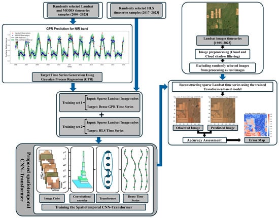
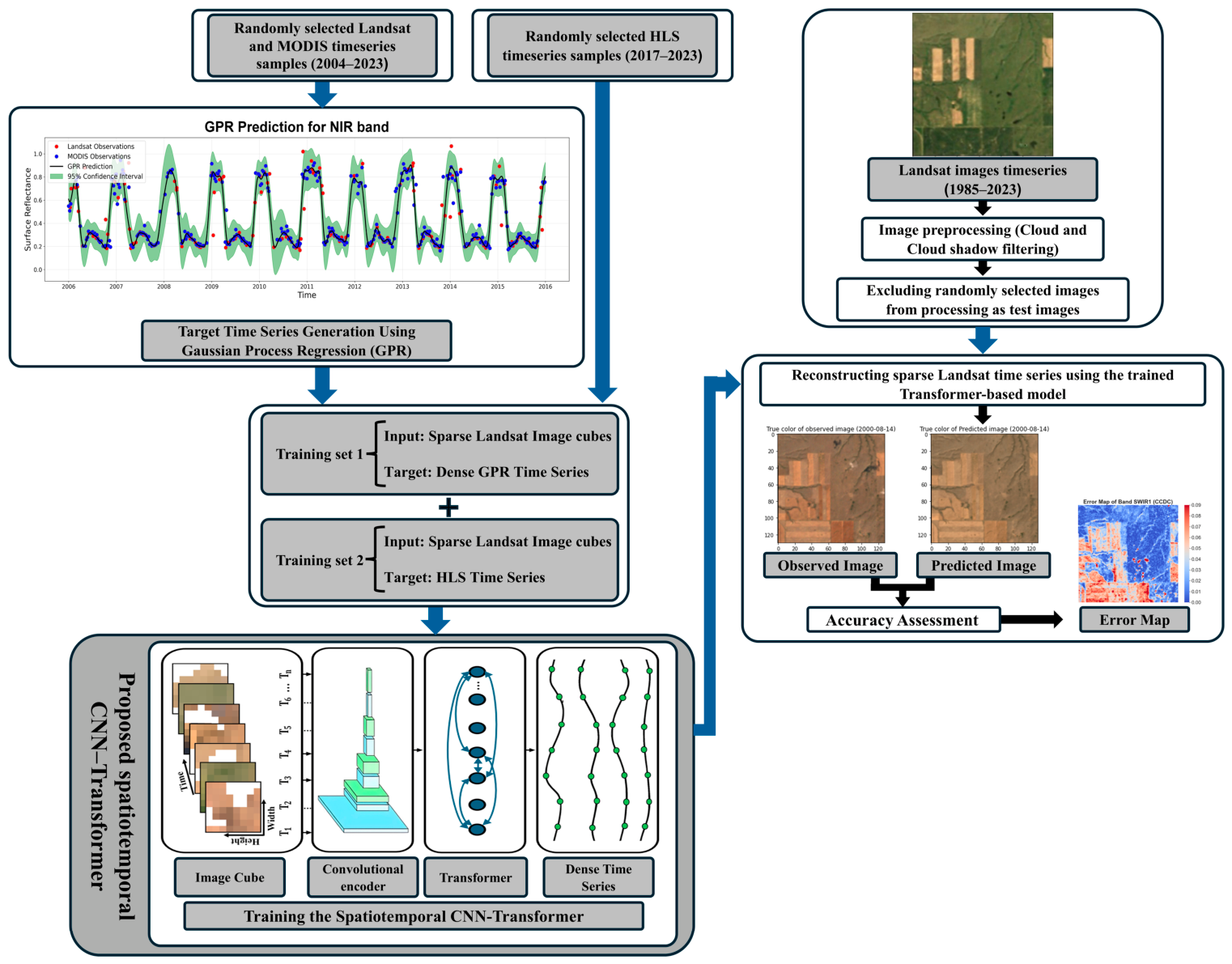
This study develops and evaluates a spatiotemporal CNN-Transformer designed to handle irregular and sparse time series for reconstructing historical Landsat data from 1985 to 2023 over a sample area in Canada’s Prairie region. It investigates whether incorporating spatiotemporal dependencies can yield more accurate and robust reconstructions than models relying solely on temporal information, particularly under challenging conditions of very sparse observations, complex landscapes, or in the presence of SLC-induced striping in Landsat 7 imagery. A flowchart summarizing the methodology is presented in Figure 1.

Figure 1. Overall technical framework of the proposed Landsat time-series reconstruction approach, including training-data preparation, the proposed spatiotemporal CNN-Transformer, and independent evaluation. Detailed architectures of individual model components are presented in subsequent figures.

2. Study Area and Dataset

The study was conducted in southeastern Alberta, Canada, within the Canadian Prairies, part of the northern Great Plains. The region is dominated by agricultural lands and grasslands but also includes multiple crop types, pasture, needleleaf and broadleaf forest, shrubland, developed areas, wetlands, water, and bare surfaces, providing heterogeneous land cover conditions. Elevations range from approximately 953 to 1083 m above mean sea level. The region exhibits pronounced seasonal dynamics driven by crop phenology, harvesting cycles, and climate variability. Together, its heterogeneous land cover composition and the 1985–2023 Landsat record provide a suitable setting for evaluating time-series reconstruction across diverse vegetation dynamics and observation conditions.

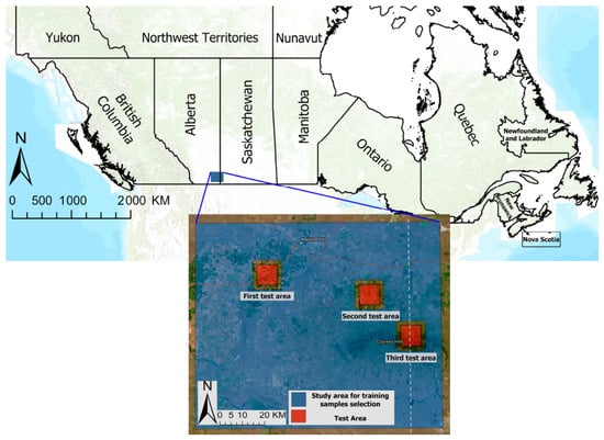
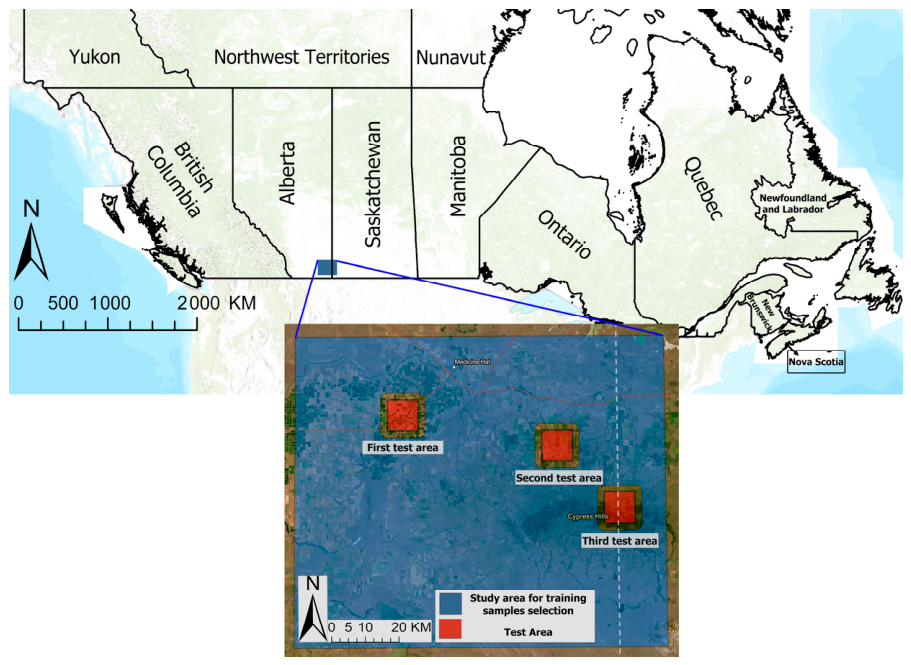
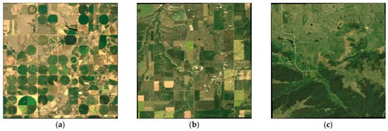
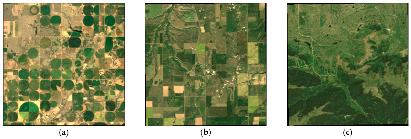
To define evaluation sites, the region was divided into 10 km × 10 km grid cells, from which three cells were randomly selected as test areas (Figure 2). To reduce spatial autocorrelation and maintain spatial independence between model development and testing, all training and validation samples were extracted at least 2 km away from the three independent test areas. The dominant land cover types in Test Areas 1 and 2 are cropland and grassland, while Test Area 3 is mainly characterized by forest, shrubland, and grassland (Figure 3).

Figure 2. The study area and its geographic location within the southern provinces of Canada. The blue region represents the area from which training samples were extracted, while the red regions indicate the three independent test areas. Basemap sources: Esri, TomTom, Garmin, FAO, NOAA, USGS, EPA, NRCan, and Parks Canada [20].

Figure 3. Overview of (a) Test Area 1, (b) Test Area 2, and (c) Test Area 3. Images shown are derived from Landsat 5 imagery acquired in July 2005.

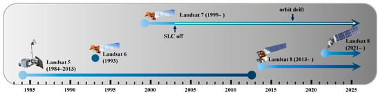
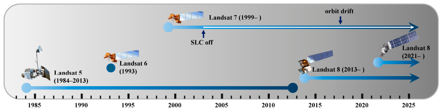
This study uses atmospherically corrected and orthorectified surface reflectance imagery from Landsat 5 (TM), Landsat 7 (ETM+), Landsat 8 (OLI), and Landsat 9 (OLI-2), covering the period 1985–2023 and accessed via Google Earth Engine. The temporal coverage and operational timelines of these Landsat missions are illustrated in Figure 4. For Landsat 7, imagery acquired after the 2003 Scan Line Corrector failure was included; however, only data up to August 2017 were used to avoid potential inconsistencies caused by orbital drift [22]. The analysis focuses on spectral bands common to all sensors in the visible, near-infrared (VNIR; 0.43–0.90 µm), and shortwave infrared (SWIR; 1.55–2.35 µm) regions at 30 m spatial resolution. Thermal bands were excluded.

Figure 4. Timeline of Landsat missions used in this study (1985–present) [17].

To support model training, two supplementary satellite datasets were incorporated. The first dataset consists of the MODIS 8-day surface reflectance products (MOD09A1.061 from Terra and MYD09A1.061 from Aqua) at 500 m spatial resolution, covering the 2004–2023 period [23]. The second dataset is the Harmonized Landsat–Sentinel-2 (HLS) product (version 2), which provides radiometrically and spatially consistent surface reflectance observations from the Operational Land Imager (OLI) onboard Landsat 8, OLI-2 onboard Landsat 9, and the MultiSpectral Instrument (MSI) onboard Sentinel-2A and Sentinel-2B at 30 m spatial resolution for the 2017–2023 period [24]. For both datasets, six spectral bands, including blue, green, red, near-infrared (NIR), shortwave infrared 1 (SWIR1), and shortwave infrared 2 (SWIR2), were used in training the deep learning models.

3. Methodology

Training targets were prepared using two complementary strategies: Gaussian Process Regression (GPR)-generated Landsat–MODIS time series provide dense temporal supervision, while HLS observations provide supervision at the 30 m Landsat scale. The Landsat image-patch sequences are then processed by a ResNet-based convolutional encoder to extract spatial–spectral information from neighboring pixels. These features are combined with the central pixel representation and subsequently processed by the Transformer to model temporal dependencies and reconstruct dense Landsat time series. After training, the models are evaluated using independent test data. The following subsections describe the baseline and proposed architectures, training data preparation, training procedure, and evaluation.

3.1. 1D Transformer Baseline

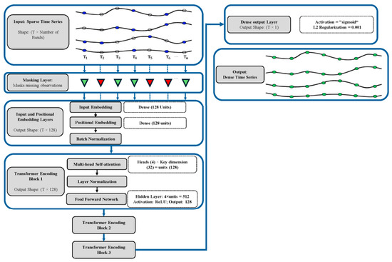
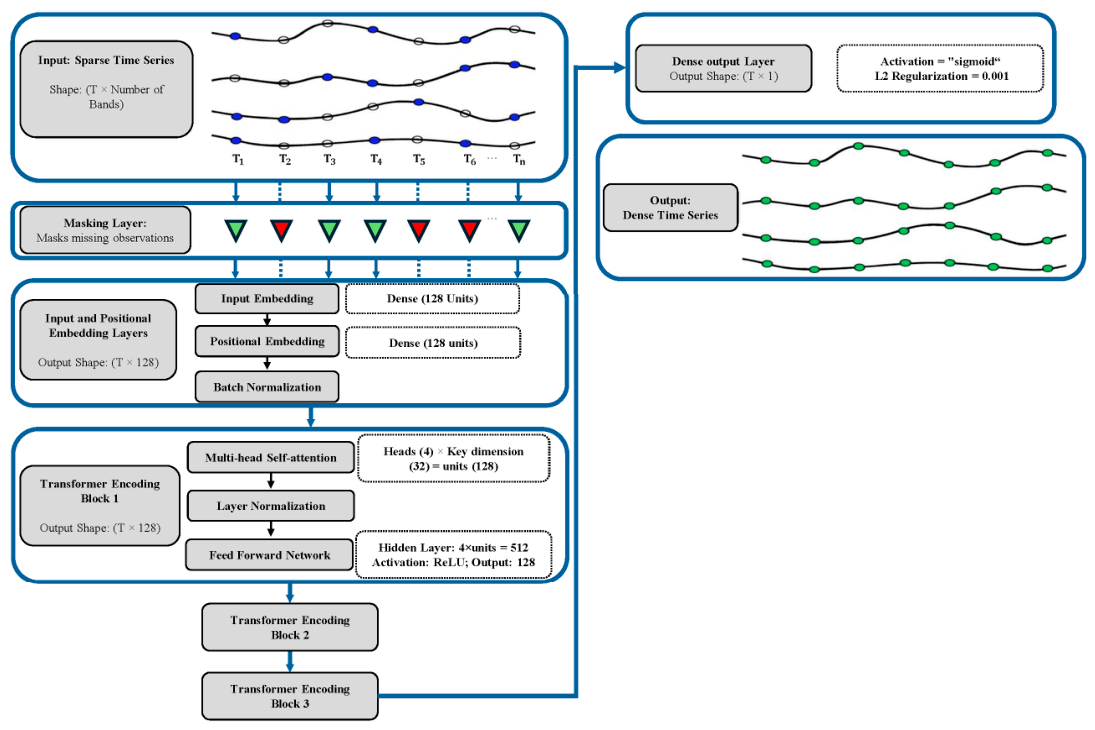
Originally developed for natural language processing [19], Transformer architectures have increasingly been applied to time series modeling because self-attention enables them to capture long-range dependencies and dynamically weight information from different timesteps [20]. Unlike recurrent architectures, Transformers model temporal relationships without sequential recurrence by combining self-attention with positional encoding. The 1D Transformer baseline used in this study consists of a masking layer, input and positional embeddings, three stacked Transformer encoder blocks, and a dense output layer, as illustrated in Figure 5.

Figure 5. Schematic of the Transformer model for Landsat time series reconstruction. Red triangles indicate invalid central pixel timesteps identified during preprocessing, including observations affected by clouds or cloud shadows. At an invalid timestep, the corresponding six-band observation is masked and excluded from Transformer processing.

As shown in the flowchart, the validity of each central pixel observation is determined during preprocessing. If the observation at a given timestep is invalid, the corresponding six-band reflectance vector is marked as missing. The masking layer uses this validity mask to exclude invalid timesteps from Transformer processing. The input embedding layer encodes each timestep into a fixed-length feature vector, to which sinusoidal positional encoding is added to represent temporal order. The Transformer comprises three stacked Transformer encoder blocks, each consisting of multi-head self-attention and feedforward layers, with four attention heads and a model embedding dimension of 128. The position-wise feedforward network within each encoder block has a hidden dimension of 512 and uses the ReLU activation function. To mitigate overfitting, a dropout rate of 0.01 was applied throughout the network, randomly disabling neurons during training. Layer normalization and residual connections are also applied to stabilize learning and enhance convergence. The final output layer is a fully connected dense layer that reconstructs the time series by predicting six values at each timestep, corresponding to the reflectance of the Landsat spectral bands (Blue, Green, Red, NIR, SWIR1, SWIR2); a sigmoid activation function constrains the predictions to the normalized valid range.

3.2. Proposed Spatiotemporal CNN-Transformer

Relative to the 1D Transformer baseline, the proposed framework introduces three main modifications. First, a convolutional encoder extracts spatial–spectral features from neighboring pixels, providing contextual information beyond the central pixel time series. Second, a patch-aware masking strategy allows a time step to contribute when sufficient valid spatial information is available, including cases in which the central pixel itself is missing. Third, the encoded spatial–spectral features are adaptively combined with the central pixel representation using learnable weights before temporal modeling. These modifications are designed to retain the temporal modeling capability of the original Transformer while providing additional spatial information under sparse or partially contaminated observations.

To capture both spatial and temporal dependencies in Landsat image time series, the Transformer framework is extended with a convolutional encoding mechanism. Each input consists of a sequence of image patches (image cubes) with dimensions T × 6 × 8 × 8, where T is the number of time steps, 6 is the number of spectral bands, and 8 corresponds to the window size. The 8 × 8 patch size was determined empirically through trial and error: smaller patches reduced reconstruction accuracy, while larger patches produced no further improvement.

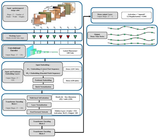
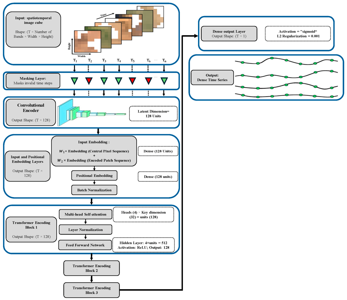
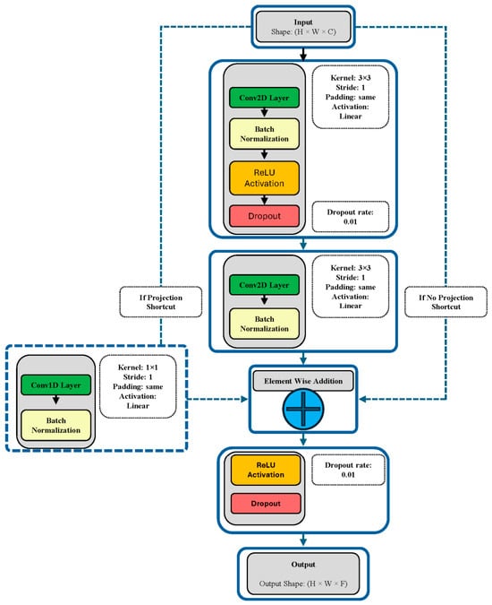
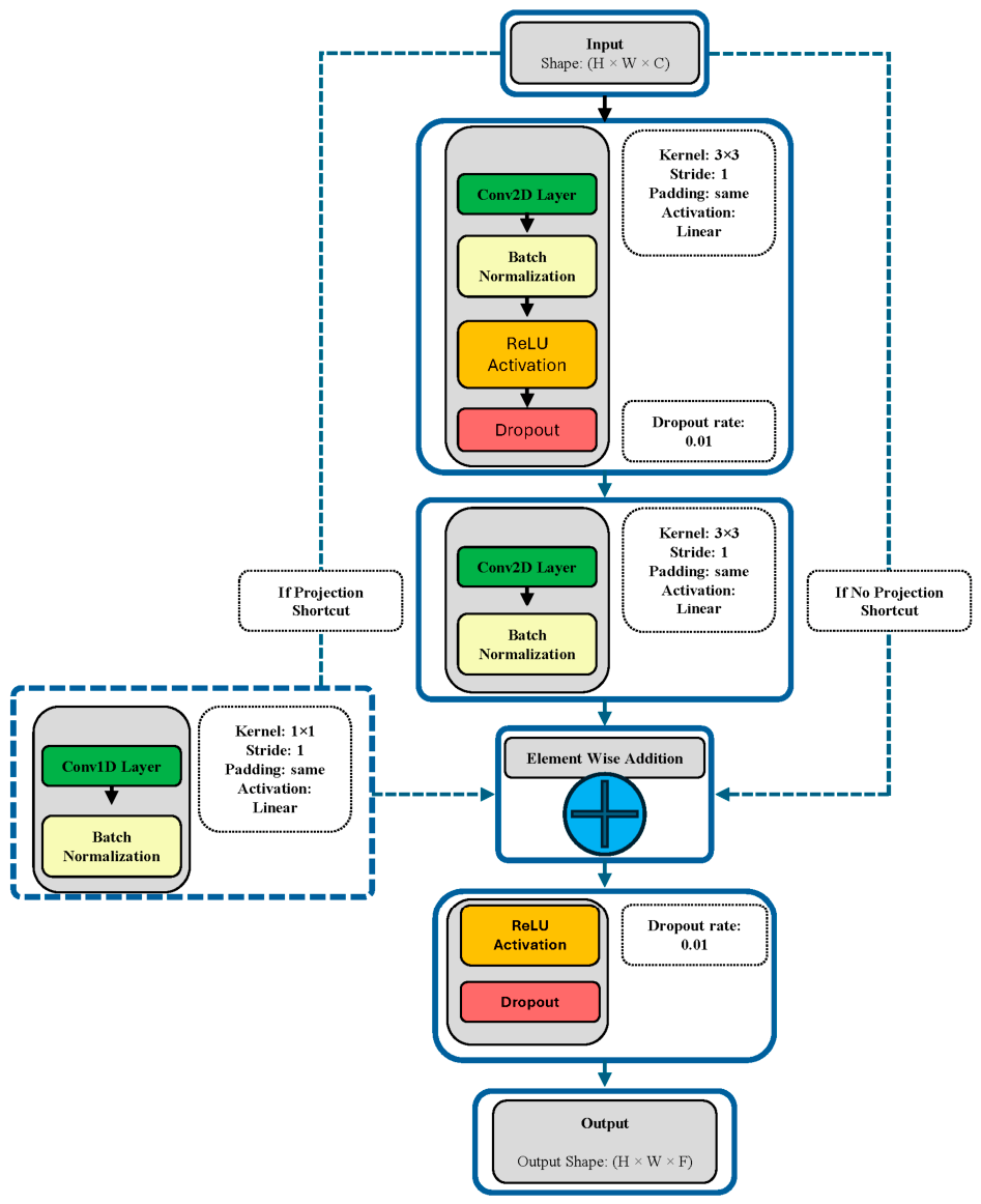
In the proposed spatiotemporal CNN-Transformer, spatial–spectral features are extracted from each image in the time series independently using a convolutional encoder applied via a Time Distributed layer. The encoder begins with a 3 × 3 convolutional layer with 32 filters, followed by three residual blocks based on the basic ResNet architecture [25], with increasing channel depth from 32 to 64 filters, interleaved with two max-pooling operations. Each residual block includes convolutional layers, batch normalization, ReLU activations, dropout for regularization, and skip connections that preserve low-level information while enabling deeper feature extraction. Spatial–spectral features are aggregated through global average pooling and projected to a 128-dimensional latent space to match the Transformer embedding size. Figure 6 provides a detailed architectural view of the proposed model, while Figure 7 and Figure 8 show the convolutional encoder and residual block components, respectively.

Figure 6. Schematic of the proposed spatiotemporal CNN–Transformer for Landsat time series reconstruction. Red triangles in the masking layer indicate invalid timesteps. For clarity, only the first Transformer encoder block is shown in detail.

Figure 7. Architecture of the convolutional image encoder. The encoder consists of an initial convolution layer followed by three ResNet blocks, two max-pooling operations, global average pooling, and a dense projection to the latent representation.

Figure 8. Residual block architecture used in the encoder. The block comprises two 3 × 3 convolutional layers with batch normalization. A projection shortcut is applied when channel dimensions differ; otherwise, an identity shortcut is used. The branches are merged by element-wise addition, followed by ReLU activation and dropout. Spatial resolution is preserved within the block.

In parallel to the encoded patch sequence, the central pixel of each patch is extracted. In contrast to the 1D Transformer, the masking condition in the spatiotemporal CNN-Transformer considers both the validity of the central pixel and the proportion of valid pixels within each patch. Specifically, a time step is considered valid and retained for further processing if either the central pixel is valid or at least 30% of the pixels in the corresponding patch contain valid observations. This masking rule is explicitly defined rather than learned by the network, and the 30% threshold was selected empirically during model development. This formulation allows the model to leverage spatial context even when the central pixel is missing, while still filtering out severely corrupted patches. Consequently, although the spatiotemporal model utilizes more data through spatial aggregation, its masking mechanism remains quality-aware by excluding time steps with insufficient valid information.

Both the encoded patch sequence and the central pixel time series are projected to the Transformer input dimension via fully connected embedding layers. To capture temporal order, a positional encoding is added to the patch embedding. The embeddings are then fused through a learned weighted sum:

Transformer Input = W₁ ∙ EmbeddedPixel + W₂ ∙ EmbeddedPatch

where W₁ and W₂ are trainable scalar weights, EmbeddedPixel is the embedded central pixel time series, and EmbeddedPatch represents the embedded spatial–spectral features. This design emphasizes the contribution of the central pixel while retaining the broader spatial context, and the learnable weights can be monitored during training to evaluate the relative importance of each component.

Importantly, after the embedding and weighted sum steps, a batch normalization layer is applied to the fused embeddings prior to the stack of Transformer encoder blocks, which are identical in the 1D Transformer and the spatiotemporal CNN–Transformer. Within each encoder block, layer normalization is applied after the self-attention and feedforward sublayers, following standard Transformer design. As the Transformer encoder blocks are identical in both models, the comparison focuses on the effect of the proposed spatial-context pathway, including both spatial–spectral encoding and the patch-aware masking strategy, rather than isolating the convolutional encoder alone. This spatiotemporal design enables effective reconstruction of Landsat time series while capturing both local spatial features and global temporal dependencies.

3.3. Landsat Time Series Reconstruction: Training and Evaluation

The Landsat time-series reconstruction workflow consists of four main stages: contaminated observation filtering, training sample preparation, model training, and evaluation. Two complementary target datasets were used for training: dense GPR-generated Landsat–MODIS time series for temporal supervision and 30 m HLS observations for Landsat-scale supervision. After training, the 1D Transformer and spatiotemporal CNN-Transformer were evaluated using independent GPR-based test time series and held-out Landsat observations. The following subsections describe each stage in detail.

3.3.1. Contaminated Observation Filtering

Cloud- and cloud shadow-affected Landsat observations were identified and masked using the commonly used Fmask object-based algorithm [26]. Although Fmask generally provides reliable screening, it can occasionally confuse clouds with transient features such as dense aerosols, smoke plumes, or flood-affected areas. Such residual uncertainties are relevant because Landsat time series may still contain noise or anomalous observations after preprocessing.

3.3.2. Training Samples Preparation

In this study, 5000 spatiotemporal image cubes were randomly extracted from the training region (blue area in Figure 2). The majority (~85%) of these were grassland and cropland, which are the dominant land covers in the study area. Sampling was stratified using the 2020 North American Land Cover 30-m dataset available on Google Earth Engine [27].

The extracted Landsat samples were temporally sparse and irregular. To train the transformer to reconstruct dense and regularly spaced time series, corresponding dense reference data were required. To address this, in the first training strategy, Landsat and MODIS observations spanning 2004–2023 (20 years) were combined and modeled using GPR to generate dense, regularly spaced targets for temporal supervision [28]. MODIS data were included as the daily coverage increases the likelihood of clear-sky observations. To maintain consistency, Landsat data were resampled to 500 m to match the resolution of the MODIS surface reflectance product.

GPR is a nonparametric Bayesian method that defines a distribution over possible functions and adjusts its complexity according to the data using Bayesian inference [29,30]. This flexibility enables GPR to capture a wide range of patterns and dependencies, making it particularly suitable for interpolating irregular time series while preserving trends and uncertainties [31].

To reduce the influence of remaining anomalous observations, the GPR reference series were generated using a two-step procedure. In the first step, NDVI was computed for each time series and modeled using GPR. Observations that deviated significantly from the modeled NDVI trajectory were identified as outliers and removed. Specifically, outlier detection was based on the GPR predictive uncertainty: observations falling outside the confidence interval (predicted NDVI ± 3σ) were excluded. This NDVI-based filtering process was performed iteratively with three iterations to progressively refine the valid observations. In the second step, the remaining observations were treated as more reliable inputs, and each spectral band was modeled separately using GPR. Band-wise modeling was also conducted iteratively, using two iterations to further filter outliers and to minimize the influence of anomalous values.

Although MODIS observations were incorporated to increase temporal density, Landsat data were prioritized because they are the primary focus of this study. Accordingly, Landsat observations were assigned a weight of 2 during GPR fitting, compared with a weight of 1 for MODIS observations. Seasonal variability was also considered through additional weighting. Winter observations were assigned a lower weight because snow cover generally introduces greater noise and uncertainty, whereas spring and fall were given greater emphasis because rapid transitional vegetation dynamics make these periods more challenging to model than summer. Based on these considerations, seasonal weights of 1, 2, and 3 were assigned to winter, summer, and spring–fall observations, respectively.

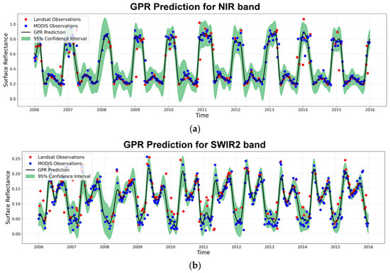
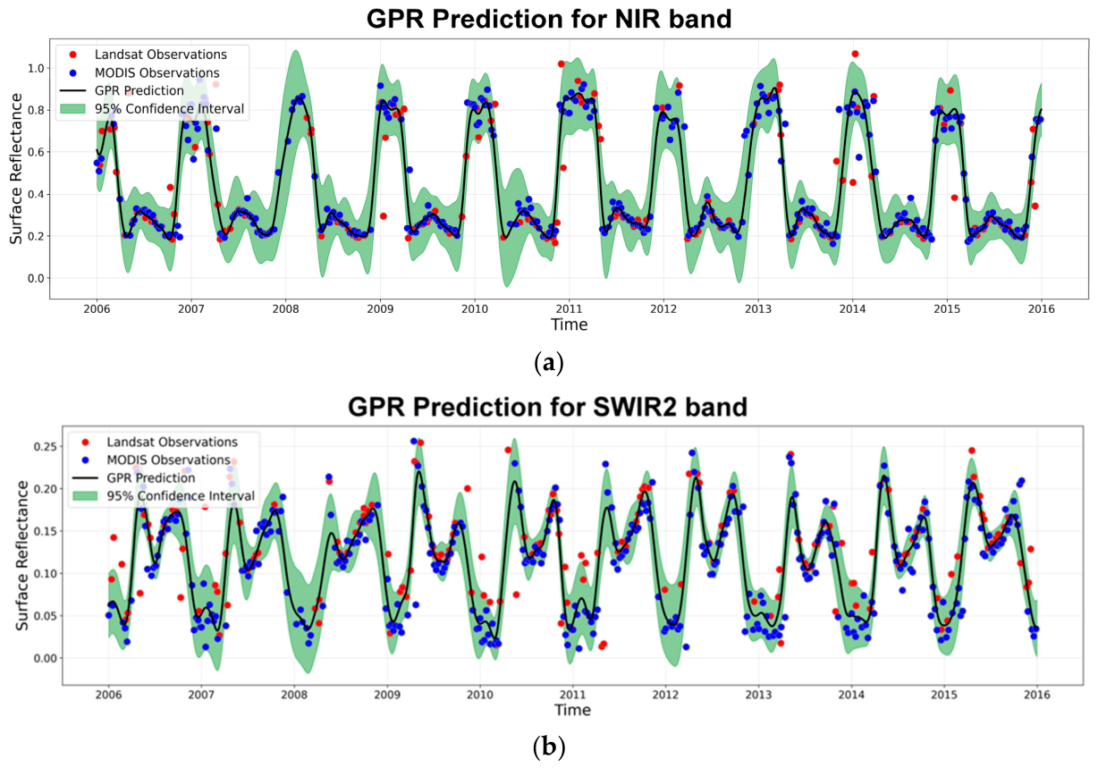
A fundamental component of GPR is the kernel (covariance function), which defines the similarity between observations and governs the smoothness, periodic behavior, and overall structure of the modeled function [32]. The adopted kernel configuration in this study consisted of a periodic kernel, a coarse-scale RBF (Radial Basis Function) kernel, a fine-scale RBF kernel, and a noise kernel. The periodic kernel was employed to model annual seasonality, using a period of 365 days and a length scale of 120 to control the frequency and smoothness of seasonal variations. The coarse-scale RBF kernel was incorporated to capture long-term temporal trends, with a length scale of 5 × 365, while the fine-scale RBF kernel accounted for intra-annual variability. The length scale of the fine-scale RBF was set to 30 for most bands, except for the SWIR bands and NDVI, where values of 20 and 50 were used, respectively. Finally, the noise kernel was included to account for random observational variability. The selection of kernel components and their characteristic scales was determined experimentally to best reflect the temporal behavior of the time series in the study area. Figure 9 illustrates an example of a grassland time series modeled using the GPR framework, showing Landsat and MODIS observations along with the modeled dense time series for the NIR and SWIR2 bands.

Figure 9. Reference time series generated using GPR for a grassland pixel in (a) NIR and (b) SWIR2 bands.

In the second training strategy, HLS time series from 2017 to 2023 (7 years) were directly employed as target data, enabling the model to learn from the Harmonized Landsat–Sentinel-2 dataset, which exhibits strong spatial and radiometric consistency with native Landsat surface reflectance observations. The use of HLS data instead of the original Landsat dataset as the training target was primarily motivated by its higher temporal density, which provides more frequent observations and facilitates more effective model training. The HLS observations therefore provided training supervision directly at the 30 m Landsat scale.

The two training strategies were used as complementary training sample sets rather than being spatially fused. The GPR-based samples were generated at 500 m to provide dense temporal targets, whereas the HLS-based samples retained the 30 m resolution of Landsat. Samples from both strategies were used during optimization of the same model, which was subsequently applied to 30 m Landsat data. The 8 × 8 patch dimension was kept fixed as the CNN input size and therefore does not represent the same physical footprint in the two strategies. At 500 m, an 8 × 8 patch covers approximately 4 × 4 km, whereas at 30 m it covers approximately 240 × 240 m. The GPR-based strategy therefore assumes some transferability of spatial–spectral information across scales, while the HLS-based strategy provides training directly at the intended 30 m Landsat scale.

To increase sample size and improve model generalization, each original time series was segmented into overlapping 5-year windows with a one-year stride. To prevent information leakage between model development subsets, the original spatial samples were split into training (85%) and validation (15%) subsets before augmentation, ensuring that all windows derived from a given sample remained within the same subset. The model is therefore trained on these 5-year segments and produces reconstructed time series of the same duration. Under this configuration, each 20-year time series in the first training strategy was divided into 16 overlapping samples, while each 7-year HLS time series was divided into 3 overlapping samples. Across the training and validation subsets, this resulted in 5000 × 16 (80,000) augmented samples for the first training strategy and 5000 × 3 (15,000) samples for the second training strategy.

Table 1 summarizes the key characteristics and configurations of each training strategy, along with the corresponding number of training samples.

Table 1. Key characteristics and complementary roles of the two training-target strategies.

Training Strategy	Purpose	Input	Target	Scale	Original Period	Number of Augmented Samples
GPR-based temporal targets	Learn dense temporal trajectories	Sparse Landsat time series	Dense GPR-reconstructed time series	500 m	2004–2023	80,000
HLS-based Landsat-scale targets	Anchor training to Landsat-scale spatial/radiometric characteristics	Sparse Landsat time series	HLS time series	30 m	1985–2023	15,000

3.3.3. Training

For model training, the central pixel of each image-cube sample served as input to the 1D Transformer, whereas the full image cube was used as input to the spatiotemporal CNN-Transformer. In the first strategy, Landsat observations were spatially aggregated to 500 m to match MODIS, whereas in the second strategy, the original resolution was maintained. To account for varying observation densities, a portion of the input observations was randomly dropped during each epoch in both training strategies, with dropout ratios randomly selected between 10% and 90%. To reduce computational load, all the time series were resampled at 7-day intervals.

To reconstruct time series longer than five years, a moving-window approach is applied, in which overlapping 5-year segments are processed sequentially, and their outputs are aggregated to form the full series. Except at the boundaries, only the three central years of each reconstructed segment are retained, as edge regions tend to be less reliable than the central portion. The choice of a 5-year segment length was determined empirically through trial and error, with this configuration yielding the best performance in terms of reconstruction accuracy and stability.

The models were trained using a weighted Huber loss [33] tailored for multiband time series data, in which each timestep is assigned a seasonally dependent weight. Winter months (December–February) were assigned a lower weight (0.5), while all other months were assigned a weight of 1.0, thereby reducing the influence of winter observations during training. Invalid values in the target time series, denoted by −2, were masked and excluded from the loss computation. This masking strategy is applied specifically to the second training dataset, which contains missing values, allowing the model to leverage only the available observations from the HLS dataset as reference data. The Huber loss improves robustness to outliers by treating small errors quadratically and large errors linearly, reducing the impact of extreme deviations. The loss is computed over all valid timesteps and spectral bands, normalized at the sample level, and subsequently averaged across the batch.

The 1D Transformer and spatiotemporal CNN–Transformer contained 629,894 and 807,912 trainable parameters, respectively. Both models were trained with the Adaptive Moment Estimation (Adam) optimizer [34], using the same training settings to enable a fair comparison between the two architectures. Training was conducted with a batch size of 5 over 100 epochs, totaling 1,615,000 iterations. All training and inference processes were carried out in Python 3.11 using TensorFlow 2.15 on an NVIDIA A30 GPU (NVIDIA Corporation, Santa Clara, CA, USA).

3.3.4. Evaluation

The performance of the models was assessed through two distinct evaluations. In the first evaluation, 1500 samples randomly selected from the test areas (red regions in Figure 2) were used as independent test data. The predictive accuracy of each model was then compared against the GPR-generated reference time series for these samples. In the second evaluation, a subset of Landsat images from test areas was reserved to enable an independent comparison of the Transformer-based models. Specifically, 15% of images from each test area were set aside, including only those with at least 60% clear observations per season to ensure reliable assessment. This threshold minimized the influence of clouds, shadows, haze, or cloud-adjacency effects, which can introduce artifacts and bias evaluation results. Based on this criterion, 141, 100, and 78 images were retained for Test Areas 1, 2, and 3, respectively. Variations in the number of eligible images across test areas are partly due to differences in cloud cover patterns but primarily reflect the distinct satellite acquisition paths, which influence revisit times, scene overlaps, and coverage frequency. Root mean square error (RMSE) was used in both evaluations as the primary metric for model accuracy. Because GPR is also used to generate one of the two training targets (Section 3.3.2), the first evaluation shows how closely each model reproduces the GPR-modeled reference rather than measured reflectance. Although the test samples come from independent areas not used in training, the reference itself remains a GPR estimate rather than an actual observation. The second evaluation avoids this limitation: the held-out Landsat images were not used, directly or indirectly, in GPR modeling or model training, and therefore provide a genuinely independent benchmark against actual observed reflectance.

For both evaluations, results were analyzed over the complete time series as well as for individual seasons: spring (March–May), summer (June–August), fall (September–November), and winter (December–February). To investigate the impact of missing observations due to clouds or shadows, 10% to 90% of the time steps were randomly removed, generating ten scenarios ranging from the original observation density to progressively sparser levels. The average annual number of clear-sky observations was also calculated to determine the minimum needed for reliable reconstruction. In the second evaluation, model performance was further analyzed across different land cover types and satellite sources. For visual inspection, predicted images, error maps showing deviations from the reference, and error histograms were generated to highlight model accuracies.

4. Results and Discussion

4.1. Time Series Reconstruction Performance (GPR-Based Evaluation)

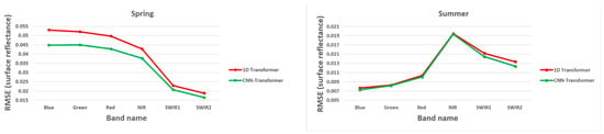
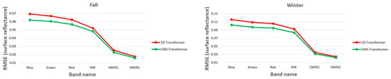
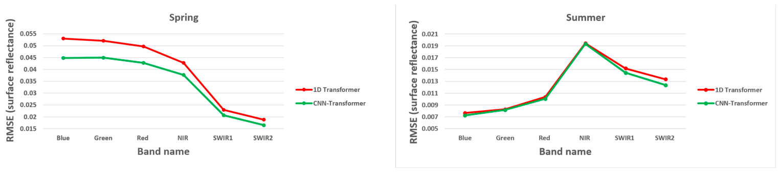
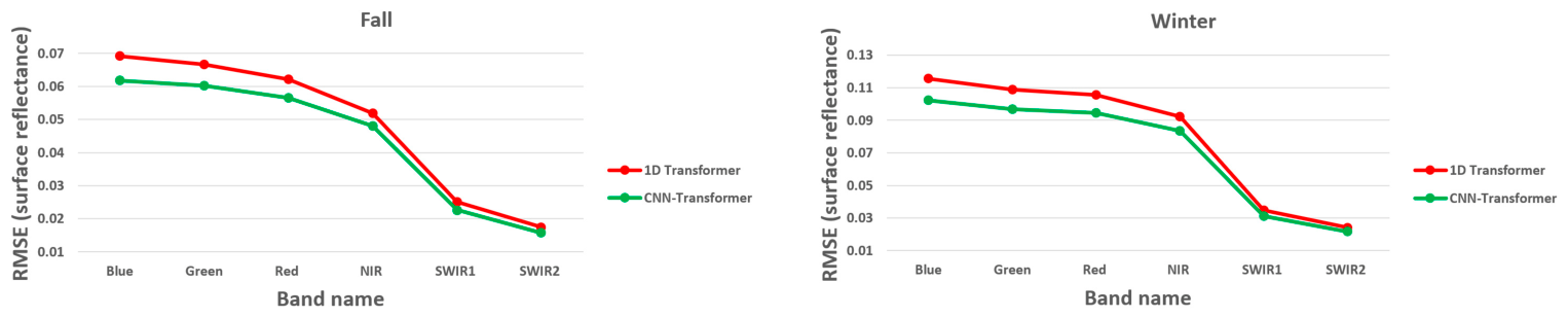
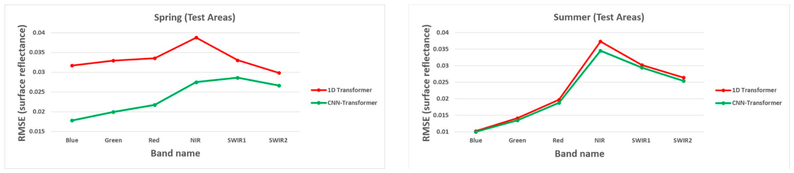
This section presents results from the first evaluation strategy, comparing the 1D Transformer and spatiotemporal CNN-Transformer reconstructions for 1500 resampled 500 m Landsat time series from the test areas against the GPR-generated reference (Table 2). As noted in Section 3.3.4, these results indicate how closely each model reproduces the GPR-modeled reference rather than measured reflectance; Section 4.2 presents the independent evaluation against actual Landsat observations. Overall, the spatiotemporal model consistently outperformed the 1D Transformer across all six spectral bands, achieving lower RMSE values for the test samples. Notably, the magnitude of improvement is relatively uniform across bands, with an average reduction in RMSE of approximately 10%. To further evaluate model performance under varying seasonal conditions, reconstruction accuracy across different seasons is summarized and illustrated in Figure 10. The results indicate that the spatiotemporal model consistently achieves higher accuracy than the 1D model across all seasons; however, the magnitude of the improvement varies seasonally. Overall, the largest performance gains are observed in spring, followed by fall and winter, whereas improvements during summer are minimal, suggesting that both models perform comparably for this season. This behavior indicates that when observation density is high and temporal variability is relatively low, the two approaches yield similar results as expected. In contrast, under conditions of sparse observations and increased temporal complexity, the spatiotemporal model demonstrates a clear advantage.

Table 2. Comparison of test sample reconstruction using the 1D Transformer and the spatiotemporal CNN-Transformer.

Band	RMSE 1D Transformer	RMSE Spatiotemporal CNN-Transformer	Improvement
Blue	0.07136	0.06292	12%
Green	0.06805	0.06055	11%
Red	0.06534	0.05839	11%
NIR	0.05709	0.05181	9%
SWIR1	0.02532	0.0229	10%
SWIR2	0.01874	0.01683	10%

Figure 10. Results of test sample reconstruction based on RMSE (GPR time series reference) for different seasons.

Figure 11 presents the reconstructed red-band time series for a representative grassland pixel over the period 2007–2012, as produced by the 1D Transformer and spatiotemporal model, along with the corresponding GPR-based reference time series. Although both approaches exhibit comparable performance over much of the time span, the spatiotemporal model provides noticeably more accurate reconstructions during intervals characterized by sparse observations, particularly in the spring of 2008 and 2010 (highlighted by the orange circles in Figure 11). This improvement can be attributed not only to the enhanced modeling capacity of the spatiotemporal model, but also to its ability to leverage spatiotemporal context by incorporating information from neighboring pixels across adjacent months.

Figure 11. Results of time series reconstruction for a sample grassland pixel from the test area using 1D (left) and spatiotemporal CNN-Transformer (right) for the red band from 2007 to 2012.

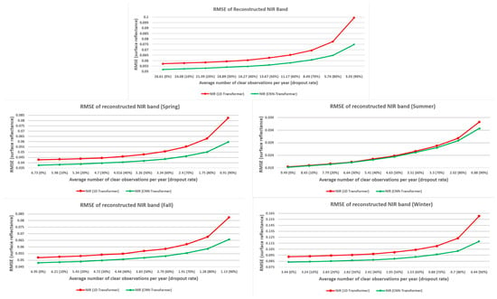
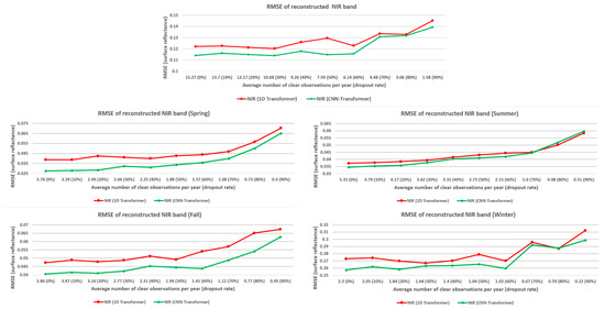
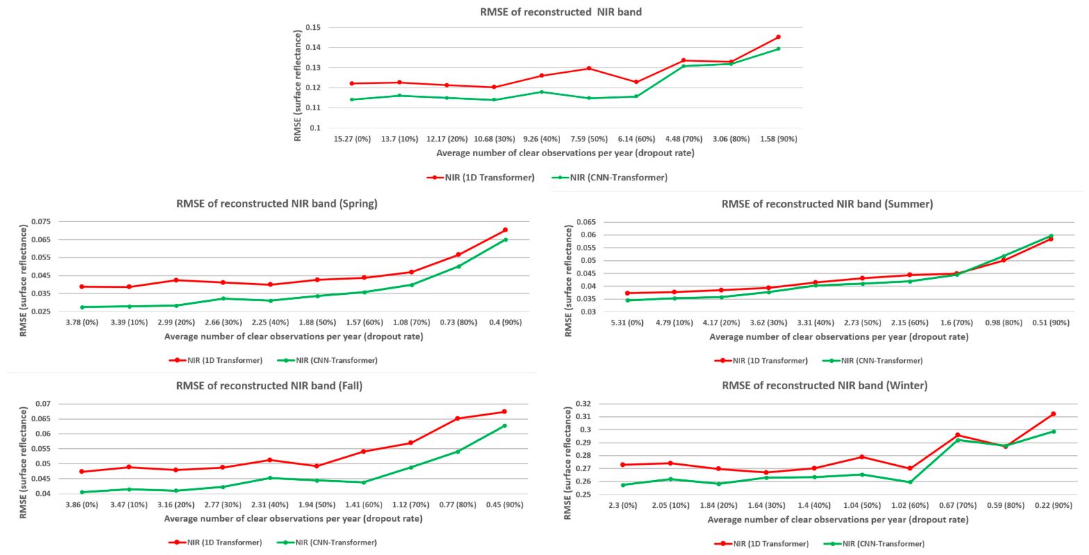
As described earlier, model performance under varying observation densities was evaluated by randomly removing between 10% and 90% of the available observations and reconstructing the resulting time series using each method. Given the similar behavior observed across spectral bands and the number of plots required to show all band and season combinations, only the NIR-band results are presented in Figure 12. Consistent with earlier findings, the smallest performance gains are observed during summer, when the time series are denser and exhibit lower temporal complexity. While increasing the dropout rate leads to higher RMSE values for both models, this degradation is more pronounced for the 1D Transformer. Moreover, the relative advantage of the spatiotemporal model becomes increasingly evident as observation density decreases, indicating that the spatiotemporal model is more robust to sparse temporal sampling compared with the 1D approach. Because the spatiotemporal framework can retain some timesteps for which the central pixel is unavailable, its performance gain reflects both spatial–spectral feature extraction and access to additional valid contextual information; separating these contributions would require a controlled common mask ablation.

Figure 12. Relation between observation density and RMSE (GPR time series reference) of test time series reconstruction.

4.2. Image Reconstruction Performance (Holdout Landsat Evaluation)

This section presents the results of Landsat image reconstruction based on the Landsat holdout images. As described in the methodology, the spatiotemporal CNN-Transformer incorporates both the encoded patch sequence and the central pixel time series. The relative contribution of these two components is controlled by trainable scalar weights learned during model optimization. After training, the optimized weights were 55.8% for the central pixel component and 44.2% for the patch sequence component. These values indicate that although temporal information contributes slightly more to the reconstruction process, spatial context also plays a substantial role, confirming the importance of integrating spatiotemporal dependencies for improved time series reconstruction.

Table 3 summarizes the reconstruction accuracy using the holdout test images from the test areas, quantified using RMSE, for both models. The results indicate that the spatiotemporal model consistently outperformed the 1D model across all three test areas. The highest reconstruction accuracy was observed for the SWIR bands, followed by the NIR, Red, Green, and Blue bands, and this performance ranking remains consistent across all study areas. The improvement rates, as reported in Table 3, vary across spectral bands and study areas, ranging from 3% to 15%.

Table 3. Comparison of test image reconstruction using the 1D Transformer and the spatiotemporal CNN-Transformer based on RMSE (holdout Landsat images).

Test Area	Band	1D Transformer	Spatiotemporal CNN-Transformer	Improvement
Test Area 1	Blue	0.13982	0.1291	8%
	Green	0.13517	0.12679	6%
	Red	0.1329	0.1255	6%
	NIR	0.12209	0.11461	6%
	SWIR1	0.05252	0.0502	4%
	SWIR2	0.04502	0.04382	3%
Test Area 2	Blue	0.17251	0.15859	8%
	Green	0.16351	0.15278	7%
	Red	0.15779	0.14898	6%
	NIR	0.14399	0.13427	7%
	SWIR1	0.05916	0.05015	15%
	SWIR2	0.04536	0.04001	12%
Test Area 3	Blue	0.14802	0.13757	7%
	Green	0.1133	0.10658	6%
	Red	0.10951	0.10351	5%
	NIR	0.10018	0.09337	7%
	SWIR1	0.03848	0.03255	15%
	SWIR2	0.02852	0.02523	12%

A more detailed evaluation was conducted to compare model performance across the three test areas under various conditions, including different seasons, land cover types, time periods, and observation densities. Although minor variations are observed among the test areas, the overall performance patterns of both Transformer models remain consistent, in agreement with the findings reported in previous analysis [20]. Consequently, given the large number of experimental scenarios and corresponding figures, the remaining analyses are summarized using performance metrics averaged across the three test areas. Exceptions are made for the single-image reconstruction examples and the spatial error analysis (Figures 16–18), which are presented for Test Areas 1 and 3.

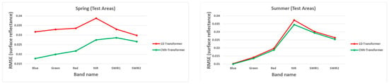
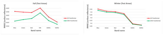
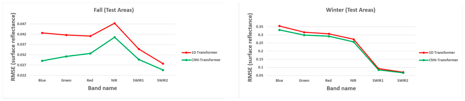
Figure 13 presents the average reconstruction accuracy of the test images across different seasons and spectral bands. Consistent with the time series reconstruction results discussed in Section 4.1, the spatiotemporal model achieves higher reconstruction accuracy than the 1D Transformer in all seasons. Summer is only slightly improved, if at all. In agreement with our previous study [20], differences between models are most evident during transitional seasons, when observation density is lower and temporal dynamics are more complex due to rapid reflectance changes in vegetated land cover types relative to summer and winter conditions. This pattern is further confirmed by the average improvement across all spectral bands: the spatiotemporal model improves image reconstruction accuracy by 29%, 4%, 20%, and 6% in spring, summer, fall, and winter, respectively.

Figure 13. Results of image reconstruction on average for test areas based on RMSE (holdout Landsat images) for spring, summer, fall, and winter.

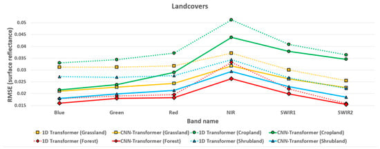
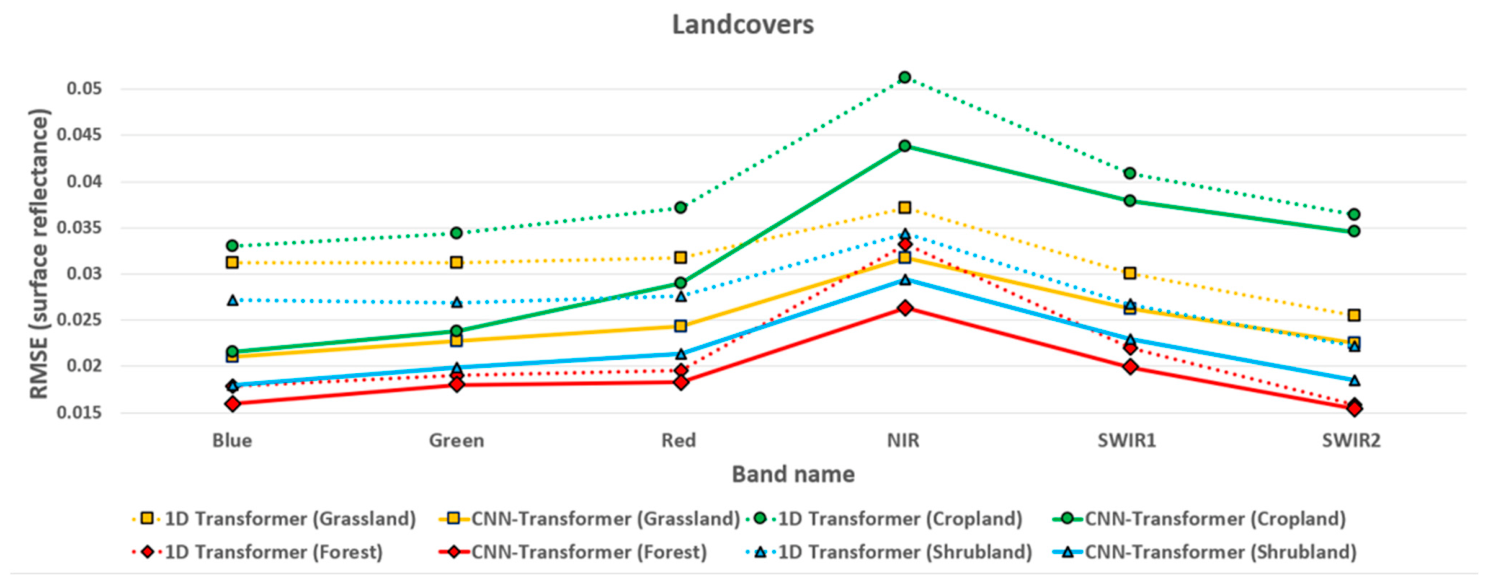
Figure 14 summarizes the average test image reconstruction accuracy, measured by RMSE, across the four dominant land cover groups represented with sufficient samples in the independent test areas: forest, shrubland, grassland, and cropland. These groups account for most of the test area pixels, although additional, less abundant land cover types are present within the broader study region. Since the study area is generally covered by snow during the winter months, including winter test images introduces additional noise and variance, which often leads to substantially higher errors. Therefore, only test images from non-winter months were used to analyze and compare the accuracy. The results indicate that both models achieve the highest reconstruction accuracy for forested areas, followed by shrubland, grassland, and cropland. This pattern is expected, as approximately 75% of the forested pixels correspond to needleleaf (evergreen) species, with the remaining portion dominated by broadleaf deciduous vegetation, resulting in relatively low temporal variability within this class. In contrast, croplands exhibit the largest reconstruction errors, reflecting their higher temporal variability and more complex phenological dynamics compared with the other land cover types. This complexity stems from the diversity of crop types and rotations across fields, each with distinct planting and harvest schedules that produce abrupt, management-driven reflectance transitions rather than the gradual seasonal changes characteristic of natural vegetation.

Figure 14. Average image reconstruction RMSE for the four dominant land cover groups in the independent test areas based on holdout Landsat images.

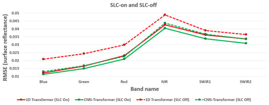
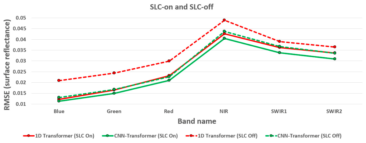
In a subsequent analysis, we evaluated the capability of each model to reconstruct Landsat time series for SLC-on and SLC-off periods. The SLC-on period was from January 1997 to December 2009, using Landsat 5 observations. The SLC-off period was from January 2004 to December 2016, using Landsat 7 imagery acquired after the SLC failure on 31 May 2003 (see Figure 4). It is also worth noting that the average number of clear observations per year was approximately 12.5 for the SLC-on period and 9.6 for the SLC-off period. This experiment was primarily designed to evaluate the robustness of each model under SLC-off conditions and to assess its ability to mitigate data gaps caused by the Landsat 7 sensor failure.

As shown in Figure 15, the spatiotemporal model consistently achieves higher reconstruction accuracy than the 1D model under both scenarios. Both approaches perform better during the SLC-on period, which is expected given the absence of striping artifacts and the greater number of clear observations compared with the SLC-off scenario. Notably, the relative performance gain of the spatiotemporal model is larger during the SLC-off period, highlighting its superior capability under more challenging conditions such as the presence of scan line artifacts. These findings suggest that the spatiotemporal model is more effective than the 1D model in mitigating the adverse effects of striping associated with the SLC-off condition.

Figure 15. Results of image reconstruction on average for test areas based on RMSE (holdout Landsat images) for SLC-on and SLC-off scenarios.

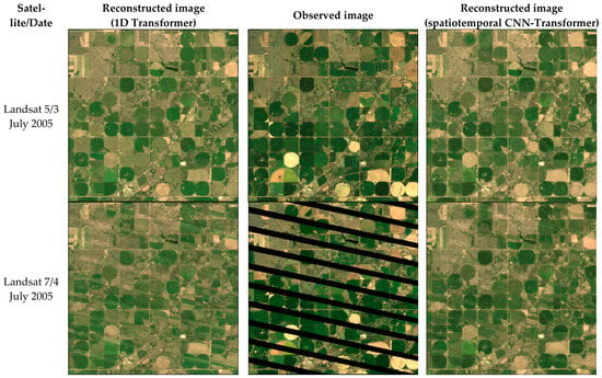
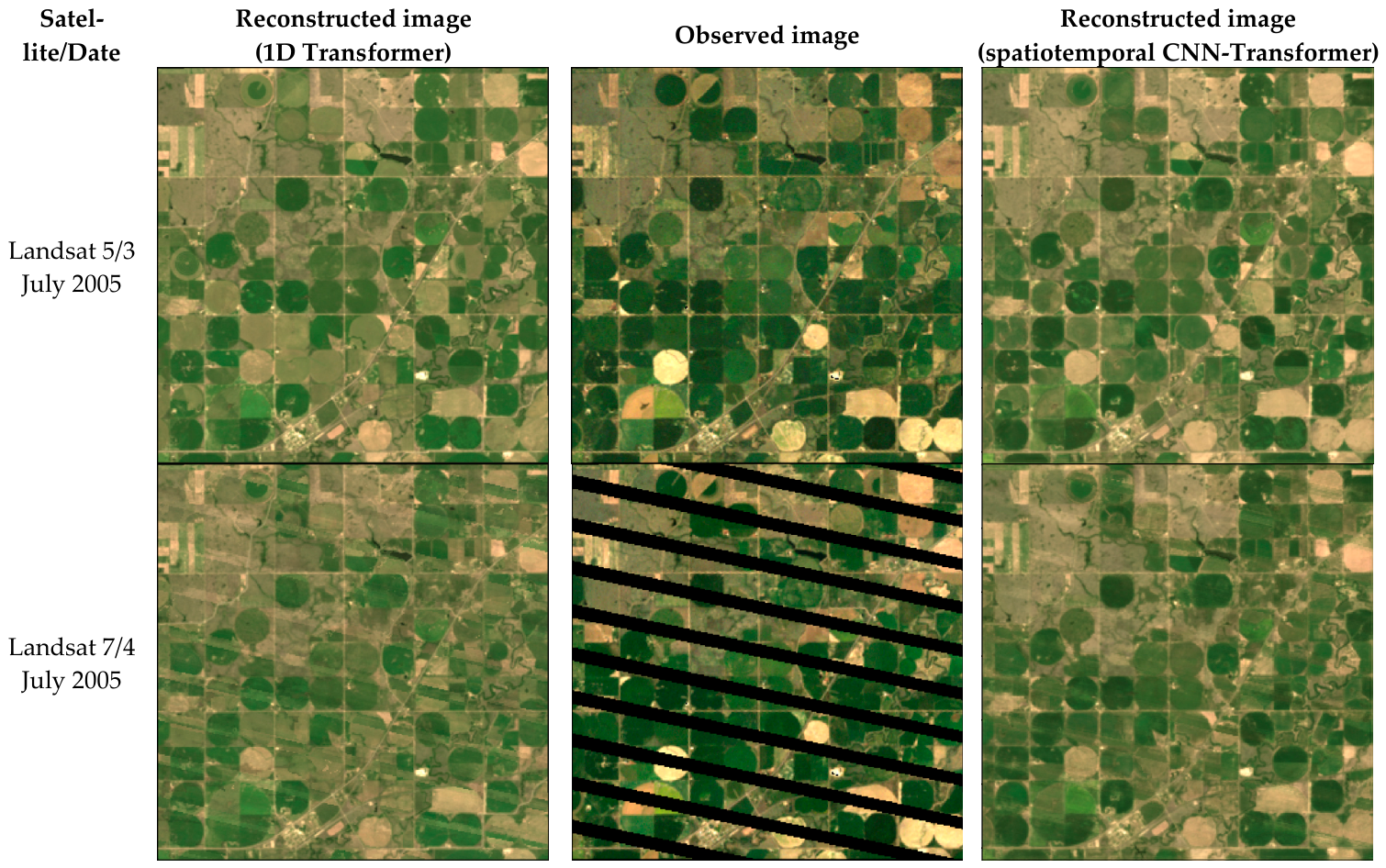
Figure 16 also presents two examples of Landsat image reconstruction using the 1D Transformer and the spatiotemporal model under SLC-on and SLC-off conditions for Test Area 1. The SLC-on example corresponds to an image acquired by Landsat 5 on 3 July 2005, while the SLC-off example was acquired by Landsat 7 on the following day, 4 July 2005. As shown, both models achieve comparable and satisfactory performance for reconstructing the SLC-on image. In contrast, for the SLC-off image, the reconstruction produced by the 1D Transformer is noticeably affected by scan line striping artifacts. Although residual striping is also present in the image reconstructed by the spatiotemporal model, this model mitigates the SLC-off effects more effectively than the 1D approach.

Figure 16. Image reconstruction results obtained using the 1D Transformer and spatiotemporal CNN-Transformer for two test images acquired by Landsat 5 (SLC-on) and Landsat 7 (SLC-off), illustrating the impact of scanline striping on model performance.

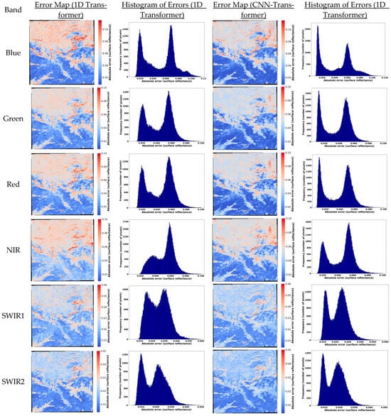
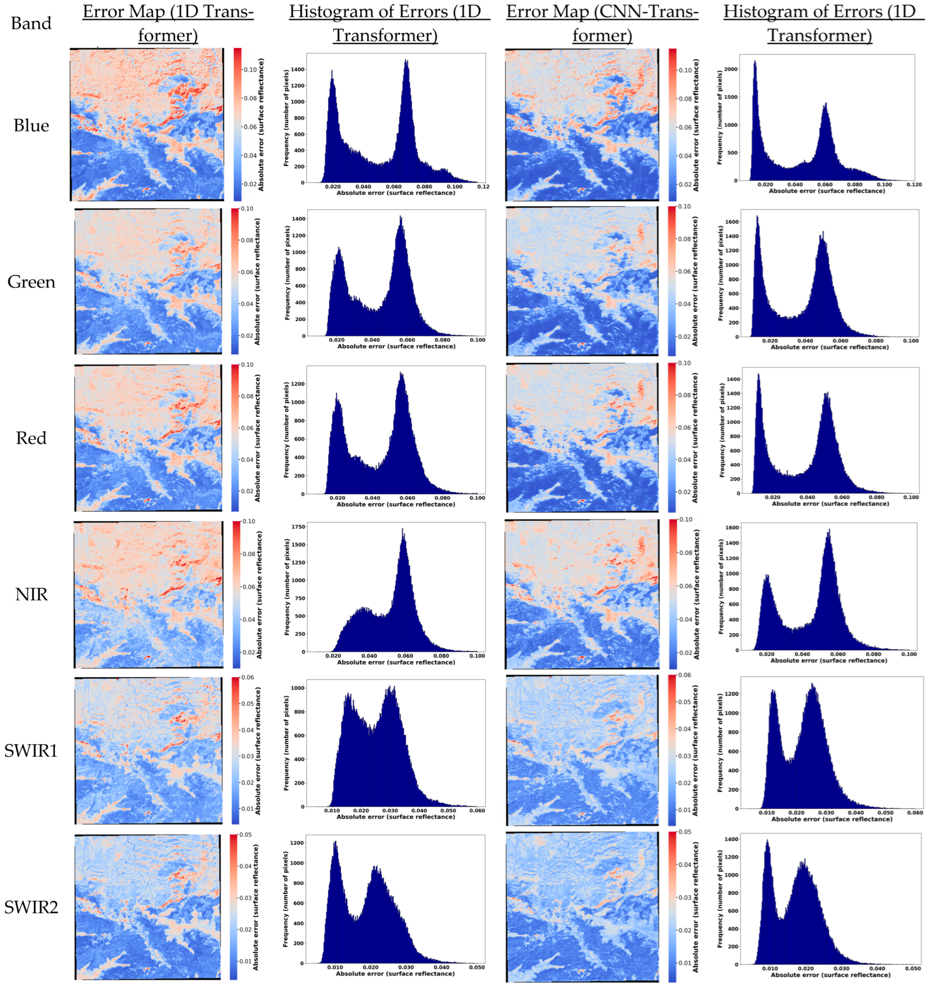
Figure 17 presents the average error maps and corresponding histograms, showing the absolute differences between the reference and reconstructed values for 78 test images from path 39 and row 25 in Test Area 3 generated by the 1D Transformer and spatiotemporal model. The results indicate that the spatiotemporal model consistently had lower reconstruction errors across all six spectral bands, as evidenced by both the spatial error patterns and the associated error distributions.

Figure 17. Average error maps and corresponding histograms of error values for reconstructed test images generated using the 1D Transformer (left) and the spatiotemporal CNN-Transformer (right).

A spatial contrast is observed between land cover types, with forested areas, predominantly located in the southern portion of the test area, generally exhibiting lower reconstruction errors than grassland and shrubland regions, which are mainly concentrated in the central and northern portions. This pattern is consistent with the land cover-specific results shown in Figure 14 and is visually apparent in the error maps. The bimodal error distributions are also consistent with spatial heterogeneity in reconstruction difficulty across the landscape; however, the histogram peaks are not explicitly assigned to individual land cover classes. More temporally stable forested areas generally show lower reconstruction errors, whereas grassland and shrubland regions tend to exhibit higher errors due to greater temporal variability and more complex reflectance dynamics. Importantly, the spatiotemporal CNN–Transformer reduces reconstruction errors relative to the 1D Transformer across the evaluated land cover types. Similar behavior has been observed in previous studies [17,20], where more temporally dynamic land covers showed greater reconstruction error.

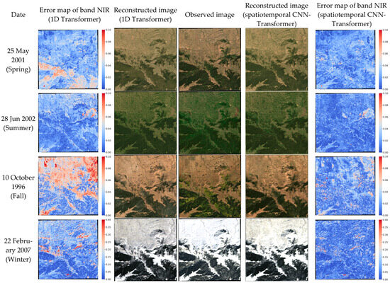
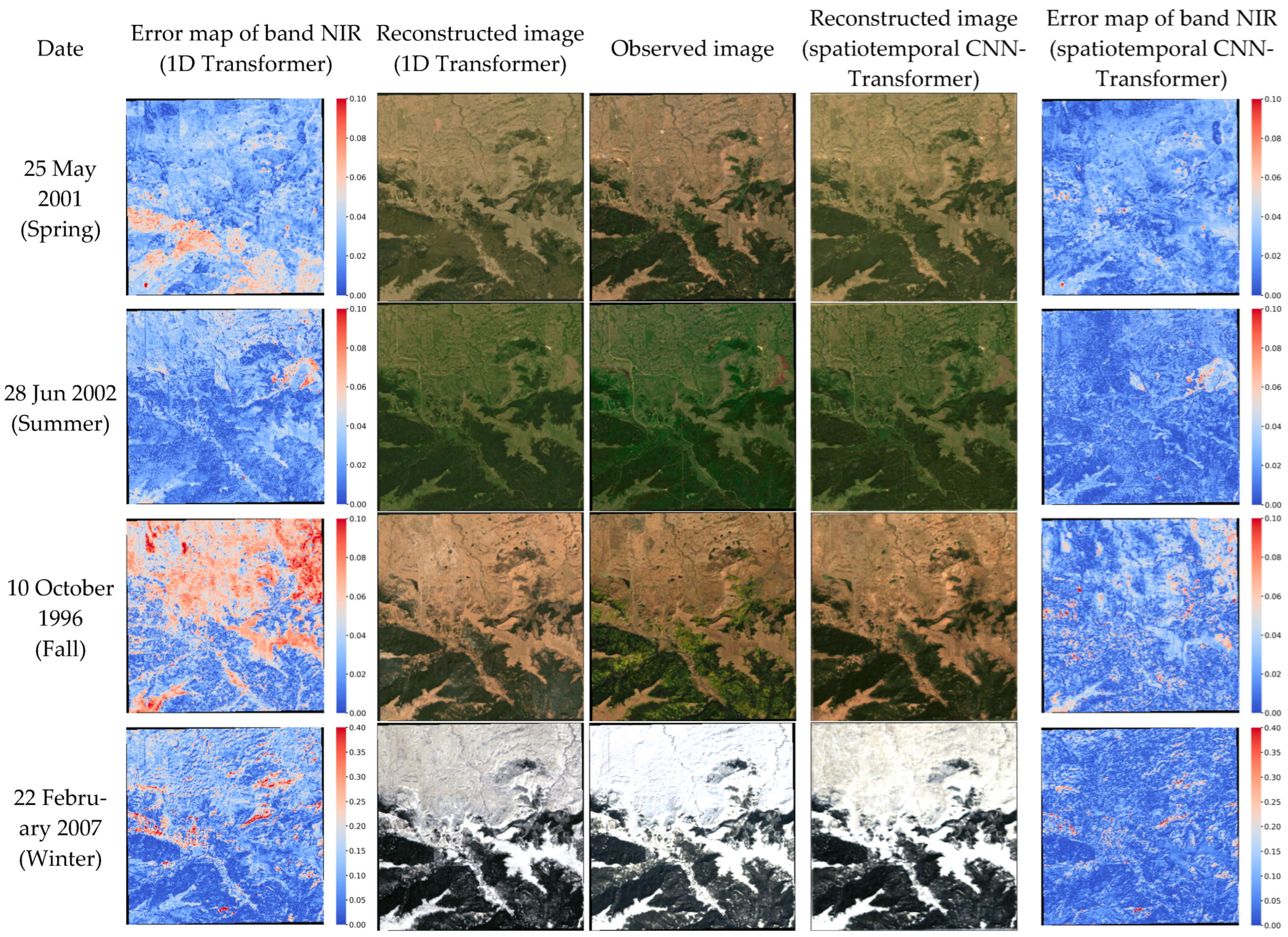
To visually assess the performance of each method further, Figure 18 presents examples of reconstructed test images across different seasons using both the 1D Transformer and spatiotemporal model. Based on the reconstructed images alone, both models appear to achieve nearly identical reconstruction performance. However, the error maps for the NIR band reveal slightly better performance of the spatiotemporal model compared to the 1D Transformer model. This difference is particularly minimal during summer, where the error maps indicate highly comparable performance between the two models.

Figure 18. Example image reconstruction and error maps using 1D Transformer and spatiotemporal CNN-Transformer for the NIR band across seasons.

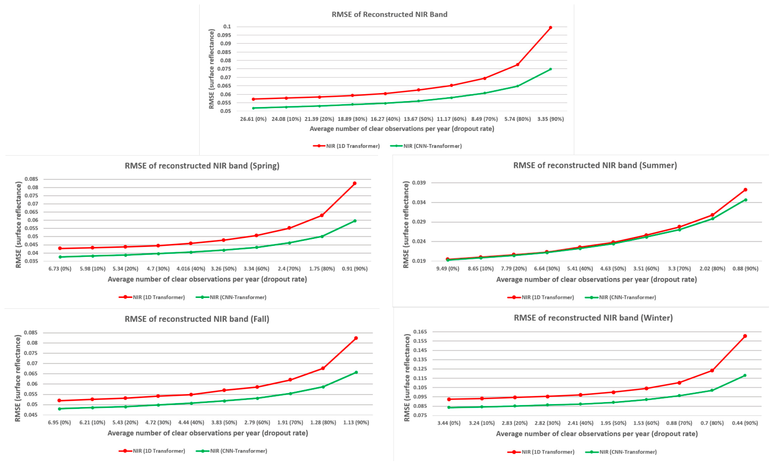
In the following, the average results of Landsat image reconstruction for the NIR band are presented across all three study areas under different observation density levels (Figure 19). As described earlier, between 10% and 90% of the available observations were randomly selected and removed, and the test images were reconstructed using the remaining observations to analyze the effect of density level on the performance of each model. Overall, the spatiotemporal model outperformed the 1D Transformer in reconstructing test images across all seasons and most density levels. Consistent with previous findings, the largest performance improvements were observed in spring and fall, followed by winter and summer. Both methods exhibited similar performance during the summer. However, at high dropout rates (80% and 90%), the 1D model was slightly better. The results also indicate that the increase in RMSE with increasing dropout rates follows a similar trend for both methods, with a pronounced rise in error once more than 60% of the observations were removed, corresponding to fewer than five clear observations per year on average. Similar results were observed for the other bands.

Figure 19. Relation between observation density and RMSE (holdout Landsat images) of test image reconstruction.

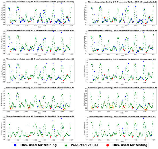
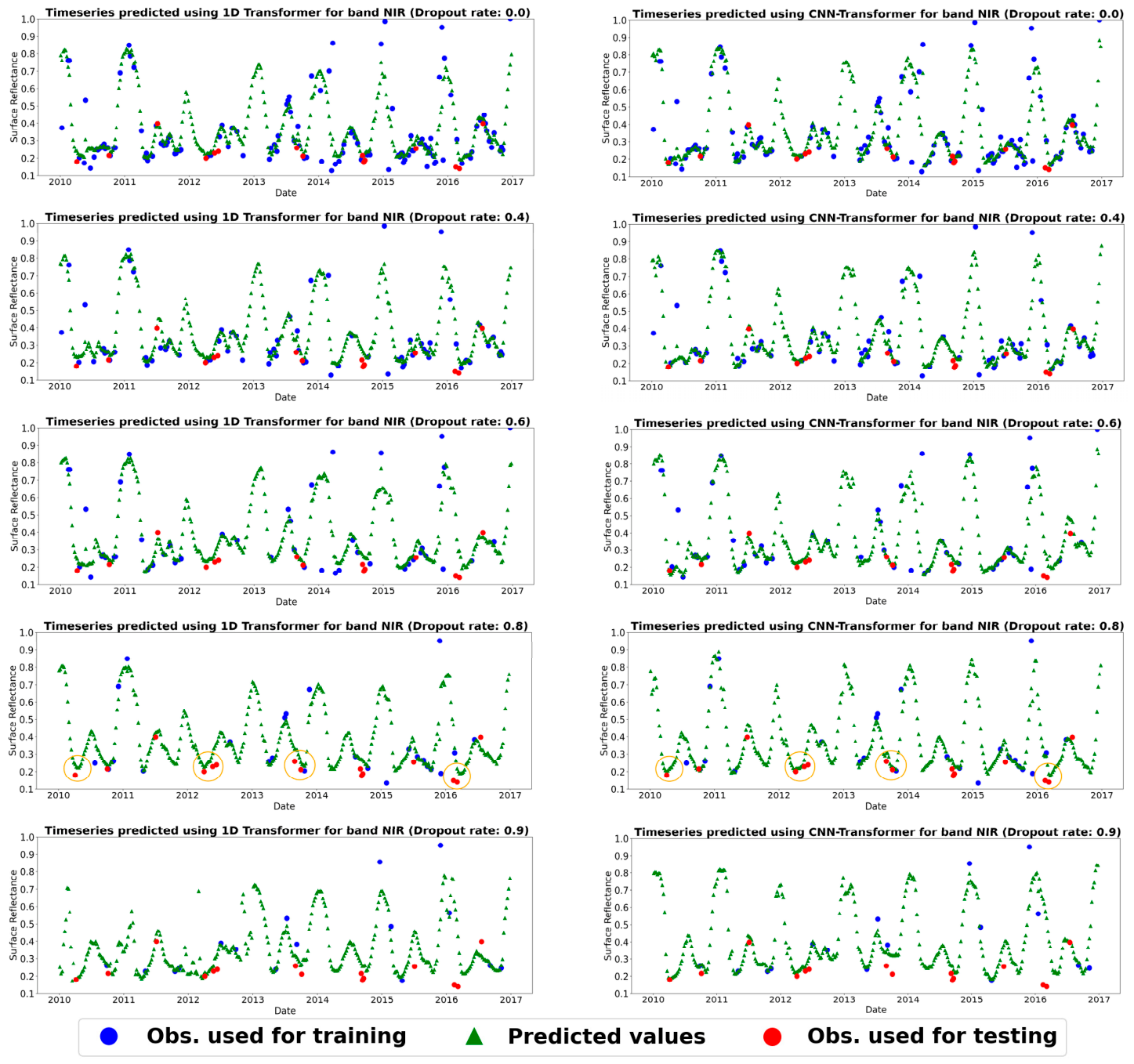
Examining the dropout results for an example single-pixel time series of cropland is shown in Figure 20. At high density levels, both methods show comparable performance in predicting test observations and reconstructing dense, regular time series. However, as the observation density decreases, the spatiotemporal model predicts test images more accurately, particularly for observations corresponding to transitional seasons (spring and fall).

Figure 20. The effect of observation density on reconstructing a sample cropland time series using 1D Transformer (left) and spatiotemporal CNN-Transformer (right) from 2010 to 2017.

For instance, at an 80% dropout rate, the spatiotemporal model clearly outperforms the 1D model in predicting test observations around spring 2010, spring 2012, fall 2013, and spring 2016, as highlighted by the orange circles. Furthermore, at a 90% dropout rate, which corresponds to fewer than two clear observations per year on average, the spatiotemporal model reconstructs the time series more accurately than the 1D model, especially during the 2010–2013 period, when the availability of clear observations is particularly limited. At this extreme sparsity level, despite the absence of clear winter observations in 2010, 2011, and 2012, the spatiotemporal model successfully preserves the overall temporal shape of the time series. This robustness can be attributed to its use of spatiotemporal contextual information from neighboring pixels, rather than relying solely on the spectral information of the central pixel.

These results support the applicability of the proposed framework within the Prairie environments represented by the training and test areas. However, the current experiments do not establish direct transferability to substantially different ecological or climatic regions. Applications to such regions should therefore be accompanied by regional evaluation and, where necessary, model retraining or adaptation using representative observations. Future work will extend model training and evaluation to a broader range of regions across Canada.

4.3. Comparison of 1D Transformer and Spatiotemporal CNN-Transformer for Computational Performance

In this section, the processing time and computational burden of each method are evaluated. Using the hardware and training configuration described in Section 3.3.3, including a batch size of 5 and 100 training epochs, the 1D model, with 629,894 trainable parameters, required 237 s per epoch (approximately 6.6 h per 100 epochs). In contrast, the spatiotemporal CNN-Transformer, with 807,912 trainable parameters, required 439 s per epoch (approximately 12.2 h per 100 epochs). Thus, the 1D model is approximately 1.85 times faster during training.

For inference benchmarking, a batch size of 200 was used. Untimed warm-up runs were performed before timing, after which inference was measured over 20 repeated runs using preloaded and preprocessed inputs. Data loading, image-patch construction, and other preprocessing operations were excluded from the timing. The resulting mean inference time per sample, for a 2028-week time series, was 91.5 ± 6.1 ms for the 1D Transformer and 193.9 ± 0.5 ms for the spatiotemporal CNN–Transformer. Thus, inference with the spatiotemporal model was approximately 2.12 times slower, consistent with the additional convolutional processing of the image-patch sequences.

The spatiotemporal model incurs higher computational costs than the 1D Transformer during both training and inference. However, beyond computational cost, data preparation and storage represent an even more substantial practical consideration. Training the 1D Transformer requires only 2D time-series inputs (time steps × six bands), whereas the spatiotemporal model requires 4D image chips (rows × columns × time steps × bands) for each sample. Preparing, downloading, and storing image chips is substantially more demanding than exporting single-pixel time series from platforms such as Google Earth Engine (GEE). For comparison, 5000 input time-series samples stored in npz format (a standard NumPy storage format) for training and testing the 1D model occupy approximately 306 MB. In contrast, 5000 image chips required for the spatiotemporal model occupy approximately 16,370 MB. The stored training dataset for the spatiotemporal model is therefore approximately 53.5 times larger than that of the 1D model. This substantial difference can lead to serious storage and data transfer limitations, particularly when training large-scale or global models that require hundreds of thousands of samples.

An important distinction of the spatiotemporal model in this study is that it operates as an image-sequence-to-point-sequence framework, where spatial context is used to reconstruct the time series of the central pixel. This design implies that, if extended to predict full image sequences (image patches) instead of individual pixel time series, the number of required model inferences could be significantly reduced. Specifically, for a chip size of 8 × 8, predictions could be generated for multiple pixels simultaneously, potentially reducing the total number of inferences by a factor proportional to the patch size. In contrast, the 1D model processes each pixel independently, requiring a separate inference for every location within the area of interest. However, generating full image-sequence predictions was not explored in this study, primarily due to challenges associated with constructing reliable target image sequences for training. In particular, residual noise sources such as clouds, shadows, haze, geolocation inconsistencies, and atmospheric effects may propagate into the target data and affect model performance. These challenges become more critical under low observation densities, where errors in both training and evaluation data can have a larger impact on reconstruction accuracy. Therefore, while the spatiotemporal model shows clear potential for more efficient large-scale inference, further investigation is required to develop high-quality spatiotemporal training datasets and to assess their influence on model performance.

5. Conclusions

This study introduced a spatiotemporal CNN-Transformer framework for reconstructing historical Landsat time series and demonstrated that incorporating spatial context substantially improves reconstruction accuracy, robustness, and stability compared with a purely temporal 1D Transformer. Across most evaluations, including GPR-based time series reconstruction, hold-out Landsat image reconstruction, seasonal analyses, land-cover comparisons, and SLC-on/off scenarios, the spatiotemporal CNN-Transformer outperformed the 1D model. The only exception was under the most extreme summer dropout conditions (80% and 90%), where the 1D model performed slightly better. The GPR-based results indicate how closely each model reproduces the GPR-modeled reference, while the holdout image results confirm that this advantage extends to actual measured reflectance. The largest gains occurred during spring and fall, when phenological transitions produce rapid reflectance changes and observation density is typically low. Under these challenging conditions, the spatiotemporal model reduced the RMSE on average across the six spectral bands by 29% and 20% for image reconstruction during the spring and fall seasons, respectively. In addition, it preserved temporal structure even when fewer than two clear observations per year were available.

The spatiotemporal model also demonstrated superior resilience to Landsat 7 SLC-off striping, producing smoother and more coherent reconstructions than the 1D model. Spatial error analyses confirmed that the spatiotemporal model reduces reconstruction errors across heterogeneous landscapes, particularly cropland areas where temporal variability was high. Although the spatiotemporal model requires substantially larger training datasets and higher computational costs during both training and inference, it offers the potential for more efficient large-scale prediction if extended to image-sequence reconstruction.

Overall, the results demonstrate that combining convolutional spatial–spectral feature extraction with temporal self-attention provides a powerful and flexible approach for reconstructing long-term Landsat time series. By effectively capturing both local spatial structure and long-range temporal dependencies, the spatiotemporal model enhances the reliability of reconstructed reflectance trajectories. This should enhance land-cover monitoring, change detection, and environmental analysis, particularly for periods with low-density observations. The model’s superior performance during transitional seasons, when phenological dynamics are most complex, suggests strong potential benefits for downstream applications that rely on spring and fall observations as key discriminatory periods. Accordingly, the performance gains reported in this study should be interpreted relative to the 1D Transformer baseline evaluated here and do not establish superiority over all existing Landsat time series reconstruction methods.

Future research will first examine the practical impact of these seasonal improvements on land cover classification and change detection workflows. A second direction will extend model training and evaluation to additional regions across Canada to assess geographic transferability and the need for regional adaptation. Further work will also focus on developing high-quality spatiotemporal training datasets and extending the model toward full image-sequence prediction to enable more efficient large-scale implementations.

References

- Wulder, M.A.; Roy, D.P.; Radeloff, V.C.; Loveland, T.R.; Anderson, M.C.; Johnson, D.M.; Healey, S.; Zhu, Z.; Scambos, T.A.; Pahlevan, N. Fifty years of Landsat science and impacts. Remote Sens. Environ. 2022, 280, 113195. [Google Scholar] [CrossRef] [Scilit]
- Wulder, M.A.; Loveland, T.R.; Roy, D.P.; Crawford, C.J.; Masek, J.G.; Woodcock, C.E.; Allen, R.G.; Anderson, M.C.; Belward, A.S.; Cohen, W.B. Current status of Landsat program, science, and applications. Remote Sens. Environ. 2019, 225, 127–147. [Google Scholar] [CrossRef] [Scilit]
- Zhu, Z.; Wulder, M.A.; Roy, D.P.; Woodcock, C.E.; Hansen, M.C.; Radeloff, V.C.; Healey, S.P.; Schaaf, C.; Hostert, P.; Strobl, P. Benefits of the free and open Landsat data policy. Remote Sens. Environ. 2019, 224, 382–385. [Google Scholar] [CrossRef] [Scilit]
- Zhu, Z.; Woodcock, C.E. Continuous change detection and classification of land cover using all available Landsat data. Remote Sens. Environ. 2014, 144, 152–171. [Google Scholar] [CrossRef] [Scilit]
- Whitney, K.; Scudiero, E.; El-Askary, H.M.; Skaggs, T.H.; Allali, M.; Corwin, D.L. Validating the use of MODIS time series for salinity assessment over agricultural soils in California, USA. Ecol. Indic. 2018, 93, 889–898. [Google Scholar] [CrossRef] [Scilit]
- Pouliot, D.; Latifovic, R. Reconstruction of Landsat time series in the presence of irregular and sparse observations: Development and assessment in north-eastern Alberta, Canada. Remote Sens. Environ. 2018, 204, 979–996. [Google Scholar] [CrossRef] [Scilit]
- Qiu, S.; Zhu, Z.; He, B. Fmask 4.0: Improved cloud and cloud shadow detection in Landsats 4–8 and Sentinel-2 imagery. Remote Sens. Environ. 2019, 231, 111205. [Google Scholar] [CrossRef] [Scilit]
- Xian, G.Z.; Smith, K.; Wellington, D.; Horton, J.; Zhou, Q.; Li, C.; Auch, R.; Brown, J.F.; Zhu, Z.; Reker, R.R. Implementation of the CCDC algorithm to produce the LCMAP Collection 1.0 annual land surface change product. Earth Syst. Sci. Data 2022, 14, 143–162. [Google Scholar] [CrossRef] [Scilit]
- Yan, L.; Roy, D.P. Spatially and temporally complete Landsat reflectance time series modelling: The fill-and-fit approach. Remote Sens. Environ. 2020, 241, 111718. [Google Scholar] [CrossRef] [Scilit]
- Tollerud, H.J.; Zhu, Z.; Smith, K.; Wellington, D.F.; Hussain, R.A.; Viola, D. Toward consistent change detection across irregular remote sensing time series observations. Remote Sens. Environ. 2023, 285, 113372. [Google Scholar] [CrossRef] [Scilit]
- Fu, Y.; Zhu, Z.; Liu, L.; Zhan, W.; He, T.; Shen, H.; Zhao, J.; Liu, Y.; Zhang, H.; Liu, Z. Remote sensing time series analysis: A review of data and applications. J. Remote Sens. 2024, 4, 0285. [Google Scholar] [CrossRef] [Scilit]
- Zhou, Y.; Wang, S.; Wu, T.; Feng, L.; Wu, W.; Luo, J.; Zhang, X.; Yan, N. For-backward LSTM-based missing data reconstruction for time-series Landsat images. GISci. Remote Sens. 2022, 59, 410–430. [Google Scholar] [CrossRef] [Scilit]
- Zhang, H.K.; Luo, D.; Li, Z. Classifying raw irregular time series (CRIT) for large area land cover mapping by adapting transformer model. Sci. Remote Sens. 2024, 9, 100123. [Google Scholar] [CrossRef] [Scilit]
- Dou, P.; Shen, H.; Li, Z.; Guan, X. Time series remote sensing image classification framework using combination of deep learning and multiple classifiers system. Int. J. Appl. Earth Obs. Geoinf. 2021, 103, 102477. [Google Scholar] [CrossRef] [Scilit]
- Zhang, Z.; Yan, J.; Liang, Y.; Feng, J.; He, H.; Cao, L. Multi-scale restoration of missing data in optical time-series images with masked spatial-temporal attention network. IEEE Trans. Geosci. Remote Sens. 2025, 63, 1–15. [Google Scholar] [CrossRef] [Scilit]
- Liu, H.; Zhang, H.K.; Huang, B.; Yan, L.; Tran, K.K.; Qiu, Y.; Zhang, X.; Roy, D.P. Reconstruction of seamless harmonized Landsat Sentinel-2 (HLS) time series via self-supervised learning. Remote Sens. Environ. 2024, 308, 114191. [Google Scholar] [CrossRef] [Scilit]
- Babadi Ataabadi, M.; Pouliot, D.; Chen, D.; Oluwadare, T.S. Landsat time series reconstruction using a closed-form continuous neural network in the Canadian Prairies region. Sensors 2025, 25, 1622. [Google Scholar] [CrossRef] [Scilit] [PubMed]
- Hasani, R.; Lechner, M.; Amini, A.; Liebenwein, L.; Ray, A.; Tschaikowski, M.; Teschl, G.; Rus, D. Closed-form continuous-time neural networks. Nat. Mach. Intell. 2022, 4, 992–1003. [Google Scholar] [CrossRef] [Scilit]
- Vaswani, A.; Shazeer, N.; Parmar, N.; Uszkoreit, J.; Jones, L.; Gomez, A.N.; Kaiser, Ł.; Polosukhin, I. Attention is all you need. In Proceedings of the 31st International Conference on Neural Information Processing Systems; Curran Associates Inc.: Red Hook, NY, USA, 2017; Volume 30. [Google Scholar]
- Babadi Ataabadi, M.; Pouliot, D.; Chen, D.; Oluwadare, T.S. Reconstructing Historical Landsat Time Series Using a Transformer-Based Deep Learning Approach: A Case Study in the Canadian Prairies Region. Can. J. Remote Sens. 2025, 51, 2603738. [Google Scholar] [CrossRef] [Scilit]
- USGS. Landsat 7. Available online: https://www.usgs.gov/landsat-missions/landsat-7 (accessed on 25 February 2026).
- Qiu, S.; Zhu, Z.; Shang, R.; Crawford, C.J. Can Landsat 7 preserve its science capability with a drifting orbit? Sci. Remote Sens. 2021, 4, 100026. [Google Scholar] [CrossRef] [Scilit]
- Vermote, E. MODIS/Terra Surface Reflectance 8-Day L3 Global 500m SIN Grid V061; NASA EOSDIS Land Processes Distributed Active Archive Center (DAAC) data set 2021, MOD09A01. 061; NASA Land Processes Distributed Active Archive Center: Sioux Falls, SD, USA, 2021.
- Masek, J.; Ju, J.; Roger, J.-C.; Skakun, S.; Vermote, E.; Claverie, M.; Dungan, J.; Yin, Z.; Freitag, B.; Justice, C. HLS Operational Land Imager Surface Reflectance and TOA Brightness Daily Global 30m v2. 0; NASA EOSDIS Land Processes Distributed Active Archive Center (DAAC) data set 2021, HLSL30. 002; NASA Land Processes Distributed Active Archive Center: Sioux Falls, SD, USA, 2021.
- He, K.; Zhang, X.; Ren, S.; Sun, J. Deep residual learning for image recognition. In Proceedings of the IEEE Conference on Computer Vision and Pattern Recognition; IEEE: New York, NY, USA, 2016; pp. 770–778. [Google Scholar]
- Zhu, Z.; Woodcock, C.E. Object-based cloud and cloud shadow detection in Landsat imagery. Remote Sens. Environ. 2012, 118, 83–94. [Google Scholar] [CrossRef] [Scilit]
- Latifovic, R.; Homer, C.; Ressl, R.; Pouliot, D.; Hossain, S.N.; Colditz, R.R.; Olthof, I.; Giri, C.P.; Victoria, A. 20 North American land-change monitoring system. In Remote Sensing of Land Use and Land Cover: Principles and Applications; CRC Press: Boca Raton, FL, USA, 2016; Volume 303. [Google Scholar]
- Pipia, L.; Amin, E.; Belda, S.; Salinero-Delgado, M.; Verrelst, J. Green LAI mapping and cloud gap-filling using Gaussian process regression in Google Earth Engine. Remote Sens. 2021, 13, 403. [Google Scholar] [CrossRef] [Scilit] [PubMed]
- Rasmussen, C.E. Gaussian processes in machine learning. In Summer School on Machine Learning; Springer: Berlin/Heidelberg, Germany, 2003; pp. 63–71. [Google Scholar]
- Gershman, S.J.; Blei, D.M. A tutorial on Bayesian nonparametric models. J. Math. Psychol. 2012, 56, 1–12. [Google Scholar] [CrossRef] [Scilit]
- Williams, C.K. Prediction with Gaussian processes: From linear regression to linear prediction and beyond. In Learning in Graphical Models; Springer: Dordrecht, The Netherlands, 1998; pp. 599–621. [Google Scholar]
- Williams, C.K.; Rasmussen, C.E. Gaussian Processes for Machine Learning; MIT Press: Cambridge, MA, USA, 2006; Volume 2. [Google Scholar]
- Huber, P.J. Robust estimation of a location parameter. In Breakthroughs in Statistics: Methodology and Distribution; Springer: Berlin/Heidelberg, Germany, 1992; pp. 492–518. [Google Scholar]
- Kingma, D.P. Adam: A method for stochastic optimization. arXiv 2014, arXiv:1412.6980. [Google Scholar]
Disclaimer/Publisher’s Note: The statements, opinions and data contained in all publications are solely those of the individual author(s) and contributor(s) and not of MDPI and/or the editor(s). MDPI and/or the editor(s) disclaim responsibility for any injury to people or property resulting from any ideas, methods, instructions or products referred to in the content. |
© 2026 by the authors. Licensee MDPI, Basel, Switzerland. This article is an open access article distributed under the terms and conditions of the Creative Commons Attribution (CC BY) license.