


Highlights
What are the main findings?
- Landscape ecological risk increased mainly during 2000–2010 and remained consistently higher on the North Korean side, with recurrent cross-border H-H adjacency identified along boundary valley sections.
- Slope was the dominant explanatory factor on both sides, whereas secondary explanatory structures differed across the border; the three 2030 land-use scenarios produced only a limited divergence in basin-wide LER.
What are the implications of the main findings?
- Recurrent cross-border H-H adjacency provides a spatial basis for prioritizing coordinated monitoring and targeted land-use management in shared boundary valley sections.
- The limited near-term scenario divergence suggests that substantial restructuring of basin-wide LER may require longer-term and spatially coordinated management rather than short-term land-use adjustment alone.
Abstract
Transboundary river basins combine spatially continuous ecological processes with nationally differentiated land use, development intensity, and environmental governance, yet it remains unclear how these asymmetries shape landscape ecological risk (LER) and whether alternative near-term land-use pathways can substantially modify the shared risk pattern. Taking the Sino–DPRK transboundary area of the Tumen River Basin as a case study, we assessed land-use and LER changes in 2000, 2010, and 2020 using a landscape-pattern-based LER index, global and local spatial autocorrelation, the geodetector, and geographically weighted regression (GWR), and simulated 2030 land use and LER under natural development (NDS), cropland protection scenario (CPS), and ecological conservation (EPS) scenarios using the Patch-generating Land Use Simulation (PLUS) model. Basin-wide mean LER increased from 0.0604 in 2000 to 0.0662 in 2010 and to 0.0666 in 2020, with most of the increase occurring during 2000–2010. In 2020, mean LER was higher on the DPRK side than on the Chinese side (0.0701 vs. 0.0646), and the combined proportion of relatively high- and high-risk units reached 40.22% and 27.03%, respectively. LER showed persistent positive spatial autocorrelation, with Moran’s I values of 0.6393, 0.6237, and 0.6347, and 55, 38, and 44 cross-border H-H adjacent pairs identified in the three periods. Slope consistently showed the highest explanatory power (q = 0.799–0.921), while the explanatory power of normalized difference vegetation index (NDVI) increased from 0.097 to 0.318; distance to roads was the strongest socioeconomic proxy (q = 0.131–0.202). GWR further indicated significant spatial non-stationarity in several major environmental relationships. For 2030, mean LER changed by +0.69%, −0.13%, and +0.60% under the NDS, CPS, and EPS, respectively, indicating only limited near-term divergence among scenarios. These results reveal persistent cross-border asymmetry together with recurrent H-H adjacency in boundary valley sections and suggest that near-term land-use adjustment alone may have limited capacity to substantially restructure basin-wide LER. The findings provide a spatial basis for prioritizing cross-border monitoring and coordinated land-use management in recurrent high-risk boundary valley segments.
1. Introduction
Land use/land cover (LULC) change is a direct manifestation of anthropogenic activities on terrestrial systems and serves as a critical driver in reshaping regional landscape patterns and ecological processes [1]. Urban expansion, agricultural development, transport infrastructure construction, and resource exploitation alter the areal proportions, patch morphology, fragmentation degree, and spatial connectivity of different land-use types, thereby further affecting ecosystem stability, continuity of ecological processes, and regional ecological security [2,3]. Landscape ecological risk (LER) assessment links land-use change, landscape patterns, and potential ecological losses, enabling the characterization of relative risk levels in ecosystems subjected to external disturbances from a spatial-pattern perspective. It has consequently become an essential tool for identifying ecological security issues and supporting land-use optimization and ecological management [4,5].
The watershed represents a critical spatial unit for conducting LER research [6]. Watersheds possess relatively integrated hydrological processes, material transport pathways, and ecological connectivity, enabling a more comprehensive reflection of the cumulative effects of land-use change on regional ecosystems [7,8]. Existing studies have conducted relatively systematic LER assessments in lake basins, mountain watersheds, arid-zone basins, and large river systems, revealing the influences of land-use change, landscape fragmentation, and anthropogenic disturbance on the spatial patterns of risk [5,9,10]. Compared with basins contained within a single nation, transboundary river basins face considerably more complex challenges [11,12]. In transboundary basins, natural processes exhibit continuity and integrity, whereas land administration systems, Ecological protection scenario policies, economic development intensities, and data availability tend to diverge under the influence of national borders [13,14]. This characteristic—continuity in natural processes juxtaposed with fragmentation in governance units—renders the formation, spatial distribution, and governance responses of ecological risk in transboundary basins more complex than those in basins confined within a single country [15,16].
To date, LER research has developed a comprehensive analytical framework integrating pattern assessment, spatial statistics, driver identification, and scenario simulation [17]. Existing studies typically construct LER indices based on land-use data, incorporating metrics such as landscape fragmentation, isolation, dominance, disturbance, and vulnerability to analyze risk patterns and their spatiotemporal dynamics [18,19]. In terms of spatial statistics, Moran’s I and local indicators of spatial association (LISA) are commonly employed to identify spatial clustering characteristics of ecological risk; the geodetector method is used to quantify the explanatory power of different factors on the spatial differentiation of risk; and geographically weighted regression can reveal the spatial non-stationarity in the relationships between risk and explanatory variables [4,20,21]. While these methods provide effective tools for understanding the spatial heterogeneity of LER, their application in transboundary basin studies still warrants further refinement. In particular, existing research has largely focused on quantifying the overall explanatory power of natural and socioeconomic factors for risk spatial differentiation, with comparatively less attention given to comparing the differences in driving structures across the two sides of the border, or to examining how national boundaries modify the spatial relationships among land-use intensity, anthropogenic activity distribution, and Ecological protection scenario effectiveness [22,23,24].
Future scenario simulation has further extended the temporal dimension of LER research. The Patch-generating Land Use Simulation (PLUS) model, which simulates land-use change through land expansion analysis and a multi-type random patch generation mechanism, has been widely applied to land-use projection under scenarios such as natural development, cropland protection, ecological conservation, and urban expansion, and further enables the assessment of ecological risk responses under different land-use pathways [25,26,27]. While these methods provide effective tools for characterizing the spatial heterogeneity of LER, applications in transboundary basins remain relatively limited. Existing studies have mainly examined historical risk evolution, spatial clustering, and environmental associations. For example, research in the Koshi River Basin compared LER among different national subregions and identified high-risk clustering near international boundaries [22], while a recent study in the transboundary Irtysh River Basin combined the geodetector and GWR to examine the overall explanatory power and spatially varying relationships of environmental factors with LER [4]. However, these studies have not simultaneously addressed cross-border differences in historical risk, side-specific explanatory structures, spatial continuity of boundary-adjacent high-risk areas, and their responses under future land-use scenarios.
Scenario-based LER studies have further evaluated ecological-risk responses under alternative land-use pathways, including natural development, cropland protection, and ecological protection scenarios [17,26,27]. However, these studies have generally been conducted within a single national or administrative setting. Consequently, it remains unclear whether cross-border risk asymmetry and spatially contiguous high-risk areas would persist under alternative development pathways in a shared basin, and whether land-use optimization concentrated on one side of the border would be sufficient to improve basin-wide risk conditions.
Previous studies in the Tumen River Basin provide an important basis for addressing this question but have focused on different ecological endpoints. Zheng et al. documented long-term wetland landscape changes and human disturbances in the Chinese portion of the basin [28], whereas Xiang et al. quantified the effects of land-cover change on ecosystem carbon stocks across the transboundary basin [29]. Other studies have revealed cross-border differences in LULC patterns and assessed ecosystem-service trade-offs under alternative future land-use scenarios [30,31]. Nevertheless, these studies have not directly examined the spatiotemporal evolution of LER, cross-boundary continuity of high-risk clusters, differences in LER explanatory structures between the Chinese and the Democratic People’s Republic of Korea (DPRK) sides, or whether such asymmetric risk patterns persist under future land-use scenarios.
To address these gaps, this study examines the Sino–DPRK transboundary area of the Tumen River Basin using land-use data for 2000, 2010, and 2020. Spatial autocorrelation analysis is used to characterize LER clustering and cross-boundary adjacency of high-risk areas; the geodetector and GWR are combined to assess the explanatory power and spatially varying statistical relationships of natural and socioeconomic factors; and the PLUS model is used to simulate LER responses under natural development, cropland protection, and ecological protection scenarios for 2030. Specifically, we address three questions: (1) How did land use and LER evolve from 2000 to 2020, and how did these trajectories differ between the two sides of the border? (2) Which factors show relatively strong explanatory power or local statistical associations with LER, and do these relationships exhibit cross-border differences? (3) How does LER respond to alternative future land-use pathways, and do cross-border risk asymmetry and boundary-adjacent high-risk patterns persist under these scenarios? The findings are expected to provide references for land-use optimization, ecological risk prevention and control, and transboundary collaborative ecological governance in the Sino–North Korean border region.
2. Materials and Methods
2.1. Overview of the Study Area
The Tumen River Basin is located in Northeast Asia and is shared by China, DPRK, and the Russian Federation (Figure 1). The main stem of the Tumen River extends approximately 525 km, of which about 510 km forms the China–DPRK boundary, and the basin covers a total area of approximately 33,000 km2. This study focuses on the Sino–DPRK transboundary area of the Tumen River Basin, encompassing parts of Jilin Province, China, and North Hamgyong Province, DPRK.
Figure 1.
Study area and spatial analysis units in the Sino-DPRK transboundary area of the Tumen River Basin. (a) Spatial distribution of major land-use types and the Tumen River within the study area; (b) geographical location of the study area in Northeast Asia, showing its position relative to China, the Democratic People’s Republic of Korea (DPRK), and Russia; (c) 5 km × 5 km landscape ecological risk (LER) evaluation grid and the subregional division used for the China–DPRK comparative analysis.
The topography of the study area is dominated by mountains, hills, and valley plains, with land-use types primarily comprising forestland, farmland, grassland, water bodies, and built-up land. The Tumen River transboundary region plays an important role in maintaining ecological security in Northeast Asia, supporting transboundary biodiversity conservation, and facilitating the ecological management of transboundary rivers. Related studies have also indicated a clear need for transboundary coordination in ecological governance in this region [32,33].
Owing to differences in topographic conditions, land-use regimes, border development intensity, and Ecological protection scenario efforts, the Chinese and North Korean sides exhibit marked disparities in land-use structure, landscape fragmentation degree, and anthropogenic activity intensity [30]. In recent years, the Chinese side has implemented relatively strong ecological conservation and forest restoration measures, resulting in a comparatively contiguous forest distribution, with built-up land and transport infrastructure primarily concentrated along river valleys and around urban nodes [34]. On the North Korean side, constrained by agricultural utilization, settlement distribution patterns, and data availability, the land-use structure along river valleys and on certain sloping areas exhibits greater uncertainty and stronger spatial heterogeneity.
2.2. Data Source
The datasets used in this study include land use, digital elevation model (DEM), temperature, precipitation, normalized difference vegetation index (NDVI), population, gross domestic product (GDP), nighttime lights, roads, and railways (Table 1). The GlobeLand30 land-use data were classified and aggregated to establish base maps of five landscape types within the Tumen River Basin: farmland, forestland, grassland, water bodies, and urban land. Slope data were extracted from ASTER GDEM 30 m resolution data using ArcGIS 10.2 software. Monthly precipitation and monthly mean temperature data from the ERA5 reanalysis dataset were selected to generate annual mean temperature and annual total precipitation data. Nighttime light data, derived from global NPP-VIIRS-like data at 500 m resolution, were employed to characterize anthropogenic activity intensity. Distances to roads, railways, and water bodies were obtained using the Euclidean distance tool.
For socioeconomic activity, this study used total GDP at purchasing power parity (PPP) rather than GDP per capita. The GDP data were obtained from the global dataset developed by Kummu et al. (2025), which provides both downscaled GDP per capita and total GDP for 1990–2022 [35]. Specifically, the 30 arc-sec total GDP (PPP) grids for 2000, 2010, and 2020 were used in this study. In the source dataset, total GDP at the grid-cell level was derived by multiplying downscaled GDP per capita (PPP) by gridded population counts. Total GDP was selected because the objective of this study was to characterize the spatial concentration of aggregate economic activity potentially associated with landscape disturbance. In contrast, GDP per capita represents average economic output per person and does not directly measure the total magnitude of economic activity concentrated within a spatial unit. Because the total GDP is itself a model-derived gridded estimate, particularly in regions with limited subnational socioeconomic statistics such as the DPRK, it was treated as a socioeconomic proxy rather than as an exact measurement of local economic output.
Land-use data were retained at 30 m or their original classification resolution for patch-level metric calculation. Population, GDP, nighttime lights, and other continuous driving-factor rasters were aggregated to the 5 km × 5 km evaluation units using unit-level summary statistics before geodetector and regression analyses.
For spatial analyses requiring metric coordinates and for cartographic presentation, all spatial layers were projected to WGS 1984 UTM Zone 52N (EPSG:32652). Unless otherwise stated, the spatial map panels use this coordinate reference system.
Table 1.
Data Sources and Notes for This Study.
Because long-term, spatially explicit, and independently verifiable socioeconomic statistics are not consistently available for the DPRK side, several socioeconomic variables used in this study should be regarded as proxy covariates rather than direct local observations. Gridded GDP represents a model-derived spatial estimate rather than observed economic output at the grid-cell level; nighttime lights provide a satellite-based proxy for illuminated human activity and do not directly measure population or economic production; and open-source road and railway vectors may vary in completeness, update frequency, and positional accuracy across countries. Population grids are likewise spatially modeled products rather than direct census observations at the 5 km evaluation-unit scale. Consequently, equal spatial coverage across the Chinese and DPRK sides does not imply equal empirical reliability. In this study, these variables were used primarily to represent relative spatial gradients in socioeconomic activity and accessibility, and their associations with LER were interpreted more cautiously than those of variables with stronger cross-border consistency and physical observability.
2.3. Research Framework
This study employs a four-step analytical framework to investigate the spatiotemporal evolution of LER and its multi-scenario future responses in the Sino–North Korean transboundary area of the Tumen River Basin for the years 2000, 2010, and 2020. First, based on GlobeLand30 land-use data, we analyzed the spatiotemporal characteristics, transition patterns, and cross-border differences in LULC change across the study area. Second, we constructed a LER assessment grid consisting of 5 km × 5 km fishing nets and calculated LER for each evaluation unit using the landscape pattern index approach (landscape vulnerability, landscape disturbance, and landscape loss indices). Subsequently, we revealed the spatial clustering characteristics of LER through global and local spatial autocorrelation analyses; we then employed the geodetector model and geographically weighted regression (GWR) to identify the dominant driving factors and their spatial non-stationarity in the spatial differentiation of LER at both global and local scales. For statistical and cross-border comparative analyses, each 5 km evaluation unit was assigned to the country that covered the majority of its area based on the principle of maximum area dominance, thereby dividing the study area into the Chinese side and the North Korean side. In the geodetector analysis, continuous driving factors were first discretized into several categories using the natural breaks method, and the q-statistic was then calculated. Finally, we simulated land-use patterns for 2030 under the natural development scenario (NDS), cropland protection scenario (CPS), and ecological protection scenario (EPS) using the PLUS model, and further evaluated the response characteristics of LER under alternative development pathways, based on which we proposed countermeasures for transboundary ecological collaborative governance and risk prevention and control. The overall analytical workflow and the relationships among the major methodological components are summarized in Figure 2.
Figure 2.
Analytical framework of this study. The workflow integrates historical LULC change analysis, LER assessment, global and local spatial autocorrelation analysis, geodetector and geographically weighted regression analyses, PLUS-based land-use simulation under three 2030 scenarios, and cross-border comparative assessment of LER.
2.4. LER Assessment
This study adopts a LER assessment approach based on land-use patterns to quantitatively characterize the relative ecological risk level of each evaluation unit under the combined effects of land-use composition, landscape spatial structure, and landscape vulnerability. This approach is capable of reflecting the relative differences in ecological risk induced by land-use pattern changes, and has been widely applied in ecological risk studies across watersheds, lakes, urban areas, and transregional contexts [4,5,18].
Following the LER assessment method of Li et al. (2024) [4], we divided the study area into 5 km × 5 km evaluation units and calculated the LER index for land-use data of 2000, 2010, 2020, and 2030 under different scenarios.
The 5 km × 5 km grid was selected as a common operational spatial support to balance the representation of local landscape heterogeneity with statistical stability and cross-period comparability. At this scale, each evaluation unit contains sufficient 30 m land-use cells to characterize land-use composition and patch configuration, while approximately 1500 evaluation units are retained for spatial autocorrelation, geodetector, and GWR analyses. The 5 km grid is therefore treated as an operational analytical scale rather than as a universally optimal resolution. Because landscape metrics and spatial statistics may vary with the size and configuration of areal units, the analysis is potentially subject to the Modifiable Areal Unit Problem (MAUP) [39]. To evaluate the scale sensitivity of the LER surface, LER was independently recalculated using 3 km × 3 km and 5 km × 5 km evaluation units while keeping the land-use data, LER formulation, and weighting parameters unchanged. The resulting LER values showed a strong Pearson correlation (), and relatively high-risk areas, independently defined as the upper 20% of LER values at each scale, exhibited 97% spatial overlap. These results indicate that the broad spatial pattern of LER was relatively stable across the two tested grid sizes; however, this comparison evaluates the scale sensitivity of the LER surface and does not demonstrate scale invariance of subsequent LISA cluster membership.
For any given study year or scenario, the LER index for the k-th evaluation unit was calculated as follows:
where denotes the LER of the -th evaluation unit; indexes the land-use type; denotes the number of land-use types; denotes the area of the -th land-use type within the -th evaluation unit; denotes the total area of the -th evaluation unit; and denotes the landscape loss index of the -th land-use type.
The landscape loss index is used to characterize the potential ecological loss of a given landscape type when subjected to external disturbances, and is jointly determined by the landscape disturbance index and the landscape ecological sensitivity-disturbance weight, with the calculation formula as follows:
where denotes the landscape disturbance index of the -th land-use type, and denotes the landscape ecological sensitivity-disturbance weight of the -th land-use type. Here, does not merely represent the natural vulnerability of the land type per se; rather, it comprehensively reflects the relative weighting of the land type in relation to ecological disturbance, landscape fragmentation, and potential ecological loss within the context of the study area.
The landscape disturbance index is derived as a weighted composite of landscape fragmentation, landscape isolation, and landscape dominance:
where , , denote the landscape fragmentation, landscape isolation, and landscape dominance of the i-th land-use type, respectively; and , , and are the weights assigned to the three landscape pattern indices, with = 0.5, = 0.3, and = 0.2 adopted in this study. These coefficients were adopted from established landscape-pattern-based LER studies that applied the same weighting scheme [4,40].
Under this literature-based parameterization, fragmentation receives the greatest weight because it directly characterizes the subdivision and discontinuity of landscape patches, isolation receives an intermediate weight because it represents the spatial separation among patches, and dominance receives a comparatively lower weight because it reflects the relative predominance of a landscape type within the overall landscape configuration. However, there is no universally accepted weighting scheme for these landscape disturbance components, and alternative weighting approaches have also been reported in previous LER studies [5]. Therefore, the adopted coefficients are treated as fixed empirical parameters rather than uniquely optimal weights. They were kept unchanged for 2000, 2010, 2020, and all 2030 scenarios to ensure internal comparability of LER across periods and scenarios.
Among them:
where is the number of patches of the -th land-use type; is the total area of the -th land-use type; is the total area of the study area; is the total number of patches of all land-use types in the study area; is the proportion of the -th land-use type area to the total study area; is the proportion of the patch count of the -th land-use type to the total patch count; and and are the weights assigned to the area proportion and patch count proportion, with = 0.6 and = 0.4 adopted in this study.
Considering the valley-type topography and land-use characteristics of the Sino–North Korean transboundary area in the Tumen River Basin, we assigned the landscape ecological sensitivity-disturbance weights for built-up land, water bodies, farmland, grassland, and forestland as 0.30, 0.25, 0.20, 0.15, and 0.10, respectively. This assignment emphasizes that built-up land in the study area is primarily concentrated along river valleys, roads, and transport corridors, and its expansion is generally associated with increased impervious surface area, riparian zone compression, and reduced landscape connectivity. Previous studies have indicated that urban expansion and increased built-up land can act as important risk sources, elevating regional LER; the increase in artificial surfaces also undermines the integrity of other landscape types and exacerbates landscape fragmentation. A higher weight was assigned to water bodies, primarily considering the sensitivity of river corridors and aquatic landscapes in the Tumen River Basin to transboundary ecological processes, floodplain risk, and ecological connectivity. A lower weight was assigned to forestland, mainly because it generally possesses higher ecological stability and stronger landscape connectivity functions.
To ensure direct comparability across historical periods and future scenarios, the LER values of all evaluation units from 2000, 2010, and 2020 were pooled and classified into five levels using the Jenks natural breaks method. A single set of thresholds was derived from the pooled dataset and then fixed for all three historical periods and the 2030 scenarios. Specifically, LER was classified as low (), relatively low (), moderate (), relatively high (), and high (). Fixing the classification thresholds across years and scenarios ensured that changes in risk-level proportions reflected changes in LER rather than changes in class boundaries.
2.5. Spatial Autocorrelation Analysis
Global and local spatial autocorrelation analyses were employed to examine the spatial characteristics of LER. The global Moran’s I index was calculated to characterize the overall spatial pattern of LER [41]:
where and denote the observed attribute values in spatial units and , respectively; denotes the local mean of the variable; denotes the mean square deviation; and denotes the spatial weight value, represented by an -dimensional matrix.
Local spatial autocorrelation was used to identify high-high (H-H) clusters, low-low (L-L) clusters, high-low (H-L) outliers, and low-high (L-H) outliers. The spatial weight matrix was constructed using first-order rook contiguity. Specifically, two 5 km × 5 km evaluation units were considered spatial neighbors only when they shared a common edge; units touching only at a corner were not considered neighbors, and no buffer-distance or distance-threshold criterion was applied. For the cross-border analysis, a cross-border H-H adjacent pair was operationally defined as two evaluation units that (1) were assigned to different countries according to the maximum-area-overlap rule, (2) shared a common edge under first-order rook contiguity, and (3) were both identified as statistically significant H-H clusters in the LISA analysis. No additional minimum cluster-size criterion was imposed. The reported pair counts therefore represent topological adjacency links rather than unique spatial areas.
Accordingly, all global Moran’s I statistics, LISA cluster memberships, H-H and L-L cluster counts and equivalent areas, and cross-border H-H adjacent-pair counts reported in this study are conditional on the 5 km × 5 km evaluation support and the associated first-order rook-contiguity spatial weight matrix.
2.6. Geographic Detector Analysis
To identify the explanatory power of natural environmental factors and socioeconomic factors on the spatial differentiation of LER, we employed the geodetector model. The fundamental premise of the geodetector is that if a given explanatory factor shares a similar spatial stratified heterogeneity with LER, then that factor possesses a relatively high explanatory power for the spatial differentiation of risk [21]. This method has been applied in studies on ecological risk, vegetation change, and watershed environmental risk [4,20]. In this study, we primarily employed the factor detector and interaction detector. The -statistic of the factor detector was calculated as follows:
where denotes the explanatory power of the LER determinant; denotes the strata of the explanatory factor; denotes the number of strata; and denote the numbers of evaluation units in stratum and in the entire study area, respectively; and and denote the variances of LER values in stratum and in the entire study area, respectively. The value ranges from 0 to 1, with a higher value indicating stronger explanatory power of the factor for the spatial differentiation of LER.
As the geodetector requires explanatory factors to be categorical variables, we discretized the continuous natural and socioeconomic factors using the natural breaks method. The factor detector was used to compare the individual explanatory power of different variables, while the interaction detector was employed to determine whether the explanatory power for the spatial differentiation of LER was enhanced or weakened after the superposition of two explanatory factors. Because the factor detector calculates the q-statistic of each explanatory factor independently rather than estimating their coefficients simultaneously in a multivariate regression framework, regression-type multicollinearity does not directly affect the individual factor-detection q-statistics [21]. Therefore, potentially correlated socioeconomic proxies, such as GDP and nighttime lights, were retained to characterize different dimensions of socioeconomic activity. Excluding either variable would not alter the single-factor q-statistics of the remaining variables, although the corresponding interaction results involving the excluded variable would no longer be available.
The interaction detector was implemented strictly as a pairwise two-factor analysis. For each pair of explanatory factors and , their categorical strata were spatially overlaid to construct , and was compared with and . Interactions were classified as bivariate enhancement when the joint q-statistic exceeded the larger of the two individual q-statistics, and as nonlinear enhancement when . No three-factor or higher-order interactions were evaluated.
Candidate explanatory variables comprised DEM, slope, temperature, precipitation, NDVI, population density, GDP density, nighttime lights, distance to roads, and distance to railways. These variables were selected a priori to represent four dimensions potentially associated with the spatial differentiation of LER: topography, climate, vegetation condition, and anthropogenic pressure and accessibility. Comparable multidimensional variable systems combining topographic, climatic, vegetation, demographic, economic, and accessibility indicators have been used in basin- and mountain-scale LER studies to characterize environmental background conditions and human disturbance [4,20,26].
DEM and slope were included because terrain constrains land-use distribution and human accessibility and is associated with erosion, geological hazards, and other disturbance-sensitive processes in mountainous landscapes [42,43]. Temperature and precipitation represent climatic conditions associated with vegetation growth and watershed ecological processes, whereas NDVI provides a spatially continuous indicator of vegetation cover and condition [4,44]. Population density, GDP density, and nighttime lights were used as complementary proxies for the intensity and spatial concentration of human activities, particularly where detailed and spatially explicit socioeconomic statistics are incomplete [45,46]. Distances to roads and railways were included to characterize spatial accessibility and potential infrastructure-related disturbance, which may be associated with land-use conversion and landscape fragmentation [4,26].
In addition to theoretical relevance, variable selection considered basin-wide spatial coverage on both sides of the border, availability for the study periods where year-specific data were obtainable, consistency of data processing, and compatibility with aggregation to the 5 km evaluation units. These variables were therefore treated as candidate explanatory factors for assessing the spatial stratified heterogeneity of LER using the geodetector.
The geodetector does not explicitly model measurement error in explanatory variables. Therefore, a high q-statistic cannot compensate for uncertainty in the underlying proxy data. Socioeconomic proxy variables were retained because they provide spatially continuous information in a data-scarce transboundary setting, but their q-statistics were interpreted as exploratory spatial associations rather than as direct estimates of the strength of socioeconomic processes. In particular, side-specific q-statistics for GDP, nighttime lights, population, and transport accessibility on the DPRK side were not assigned the same evidential confidence as results derived from variables with more consistent cross-border observation and validation.
2.7. Geographically Weighted Regression Analysis
To further characterize spatial variations in the statistical relationships between LER and the primary explanatory variables, we employed geographically weighted regression (GWR). Unlike global regression models that assume spatially invariant coefficients, GWR allows regression coefficients to vary across locations and can therefore reveal local differences in the direction and magnitude of statistical associations between LER and explanatory variables [47]. This approach has been applied to investigate spatially varying relationships associated with LER in previous studies [4]. The GWR model is expressed as:
where denotes the LER value of evaluation unit ; denotes the spatial coordinates of evaluation unit ; denotes the local intercept term; denotes the local regression coefficient of the -th explanatory variable at the location of evaluation unit ; denotes the -th explanatory variable of evaluation unit ; and denotes the random error term.
The variables entering GWR were selected from the broader factor set used in the geodetector analysis by considering their geodetector performance, physical interpretability, spatial resolution, cross-border data consistency, and suitability for local regression. The geodetector analysis included slope, DEM, temperature, precipitation, NDVI, population, GDP, nighttime lights, distance to roads, and distance to railways. Among these variables, slope, DEM, temperature, and NDVI were retained in the final GWR models because they provide continuous basin-wide spatial coverage, have direct physical interpretations in relation to terrain, climatic conditions, and vegetation status, and have comparatively consistent data quality across the Chinese and DPRK sides. Their inclusion also allowed the local regression to focus on environmental relationships that could be compared consistently across the three study periods.
The remaining variables were retained in the geodetector analysis but were not incorporated into the final GWR specification for different reasons. Population, GDP, and nighttime lights were used as complementary proxies of socioeconomic activity in the broader explanatory analysis; however, their gridded estimates on the DPRK side involve greater uncertainty because detailed subnational socioeconomic observations are limited and the corresponding products rely partly on spatial downscaling or remote-sensing proxies [35,45]. Distance to roads and distance to railways were retained as transport-accessibility factors in the geodetector analysis, but were not included in the final local regression because the completeness and positional consistency of open transport-network data may vary across the two sides of the international boundary. Precipitation was also retained in the geodetector analysis but was not introduced into GWR because its native spatial resolution of approximately 0.25° is substantially coarser than the 5 km evaluation units and its single-factor q-statistics were consistently low in the present study. These exclusions do not imply that the corresponding factors are ecologically irrelevant; rather, the geodetector was used to compare their basin-wide explanatory power and interactions, whereas GWR was restricted to a smaller set of variables with more consistent spatial support for examining local statistical relationships.
Before final GWR specification, ordinary least squares regression was used as a diagnostic screening step, and multicollinearity was examined for six continuous candidate variables: distance to roads, distance to railways, temperature, DEM, slope, and NDVI. Variance inflation factors (VIFs) were used to assess global multicollinearity because excessive collinearity can destabilize the estimation and interpretation of local regression coefficients [48]. The VIF values of distance to railways, distance to roads, temperature, DEM, slope, and NDVI were 1.109, 1.551, 3.939, 4.062, 1.670, and 1.029 in 2000; 1.109, 1.631, 3.414, 3.362, 1.641, and 1.029 in 2010; and 1.111, 1.468, 4.203, 4.473, 1.682, and 1.029 in 2020, respectively. All VIF values were below 5, indicating that serious global multicollinearity was not detected. In particular, the low VIF values of distance to roads and distance to railways indicate that their exclusion from the final GWR models was not attributable to multicollinearity.
Accordingly, population, GDP, nighttime lights, distance to roads, and distance to railways were not included in the final GWR specification. This exclusion was not intended to imply ecological irrelevance; rather, it was an explicit uncertainty-control decision intended to prevent comparatively uncertain cross-border socioeconomic proxies from directly determining local regression coefficients. The final GWR inference therefore relies on variables with comparatively greater spatial continuity and cross-border consistency.
The GWR models were implemented in ArcGIS Pro using a Gaussian kernel and an adaptive nearest-neighbor bandwidth. Independent optimization based on the corrected Akaike information criterion (AICc) produced optimal bandwidths of 14, 16, and 15 nearest neighbors for 2000, 2010, and 2020, respectively. To improve the comparability of local coefficient patterns among the three periods, a common adaptive bandwidth of 15 nearest neighbors, equal to the arithmetic mean of the independently optimized bandwidths, was used in the baseline models. Under this adaptive specification, the number of neighboring observations was held constant, whereas the geographic extent of the kernel varied according to the local spatial density of observations. Bandwidth sensitivity was further examined using alternative bandwidths ranging from 10 to 30 nearest neighbors. The principal spatial distributions of the local coefficients and local R2 remained qualitatively consistent across these specifications, indicating that the main spatial patterns were relatively stable within the tested bandwidth range.
To formally determine whether the observed spatial variation in local coefficients exceeded that expected under a spatially stationary relationship, Monte Carlo spatial variability tests were conducted with 999 random permutations using the GWmodel package in R [49]. The tests employed the same Gaussian kernel, common adaptive bandwidth of 15 nearest neighbors, and WGS 1984 UTM Zone 52N coordinate system as the baseline GWR models. A p-value below 0.05 was interpreted as statistical evidence that the corresponding local coefficient exhibited significant spatial variability [47]. Model performance was further characterized using R2, adjusted R2, AICc, and local R2. The GWR coefficients were interpreted as spatially varying statistical associations rather than as estimates of causal effects.
2.8. PLUS Model and 2030 Multi-Scenario Simulation
To simulate land-use patterns under alternative development pathways for 2030, we employed the PLUS model. PLUS integrates a Land Expansion Analysis Strategy (LEAS) with a Cellular Automata model based on multi-type Random Patch Seeds (CARS). LEAS identifies the expansion of individual land-use types between observed periods and estimates their relationships with explanatory factors using a random forest algorithm, whereas CARS allocates future land-use changes according to land-use demand, transition constraints, neighborhood effects, and land-development probabilities [25]. The PLUS model can be expressed as:
where denotes the growth probability of LULC type on cell ; is a vector composed of multiple driving factors; (·) is the indicator function of the decision tree set; is the predicted type of the -th decision tree for ; is the total number of decision trees; takes a value of either 0 or 1; is the overall probability of LULC type ; is the growth probability surface of LULC type ; is a random number in the range [0, 1]; is the threshold for generating new LULC patches of type ; is an adaptive drive coefficient dependent on the difference between the current land quantity at iteration and the target demand for LULC type ; and denotes the neighborhood effect for cell , expressed as the proportion of LULC type within the surrounding neighborhood.
The model was calibrated using the 2000 and 2010 land-use maps to simulate the 2020 land-use pattern. Comparison between the simulated and observed 2020 maps yielded a Kappa coefficient of 0.8035 and an overall accuracy of 92.75%, indicating adequate agreement for subsequent scenario simulation. The 2010–2020 land-use changes were subsequently used to derive recent expansion rules. The LEAS module incorporated ten driving factors, including DEM, slope, temperature, precipitation, NDVI, population, GDP, nighttime lights, distance to roads, and distance to railways.
Several socioeconomic inputs to LEAS, including gridded GDP, population, nighttime lights, and transport-network variables, are proxy-based on the DPRK side and therefore introduce additional uncertainty into the estimated land-expansion probability surfaces. Historical validation of the PLUS model evaluates the integrated ability of the full model to reproduce the observed 2020 land-use pattern; it does not independently validate the accuracy of each socioeconomic proxy or eliminate uncertainty in the corresponding development-probability estimates. Accordingly, the 2030 outputs are interpreted as conditional scenario projections under the adopted data and constraints rather than deterministic forecasts of future land use.
Three scenarios were developed by jointly modifying 2030 land-use demand and CARS conversion constraints. The NDS continued recent land-use transition tendencies without additional scenario-specific conservation restrictions beyond the baseline conversion matrix. The CPS prioritized cropland retention. Relative to the historical Markov transition probabilities, the probability of cropland conversion to built-up land was reduced by 60%, and direct farmland-to-built-up conversion was prohibited during CARS allocation. The EPS prioritized the retention and expansion of ecological land. The probabilities of farmland conversion to forestland and grassland were each increased by 30%, while farmland conversion to built-up land was reduced by 30% and forestland and grassland conversion to built-up land were each reduced by 50%. During CARS allocation, existing forestland, grassland, and water bodies were protected from conversion to other land-use classes, whereas farmland was allowed to convert to ecological land but not to built-up land. The quantitative 2030 land-use demand targets are presented in Table 2, and the complete scenario-specific conversion matrices and Markov adjustments are provided in Tables S1 and S2. Land-use demand values represent scenario-specific Markov demand targets used as quantitative constraints in the PLUS simulations. Because spatial allocation is additionally subject to the CARS conversion matrices, the realized simulated land-use areas may differ slightly from the target demands.
Table 2.
Land-use demand targets and common CARS parameter settings for the 2030 PLUS simulations.
Non-scenario-specific CARS parameters were held constant across all three simulations. Land-use-specific neighborhood weights were manually calibrated with reference to previous PLUS applications and the historical expansion characteristics of the study area to represent differences in neighborhood expansion potential among land-use types [26]. The neighborhood weights were 0.168565 for farmland, 0.776067 for forestland, 0.032837 for grassland, 0.006560 for water bodies, and 0.015971 for built-up land. The expansion coefficient was set to 0.01, the percentage of seeds to 0.05, and the default 3 × 3 Moore neighborhood was used. The cellular automata procedure was allowed to run for a maximum of 100 iterations and terminated earlier when the difference between the simulated land-use cell quantity and the corresponding Markov demand was less than two cells. Keeping these parameters constant ensured that differences among the three simulations primarily reflected scenario-specific land-use demand and conversion constraints.
The three scenarios should be interpreted as conditional land-use projections under predefined development and conservation assumptions rather than as estimates of causal policy effects. After obtaining the 2030 land-use maps, LER was recalculated using the same assessment formulation and fixed risk-class thresholds applied to the historical periods, thereby ensuring direct comparability between historical and scenario-based risk patterns.
2.9. Cross-Border Regional Comparison and Evaluation of Unilateral Protection Contribution
To analyze the differences in LER between the Chinese and North Korean sides, we assigned each evaluation unit to either the Chinese side or the North Korean side based on the principle of maximum area overlap with the national boundary. For each side, we separately compiled statistics on land-use structure, area proportions of risk grades, mean risk index, area of high-risk zones, and risk transition patterns.
Based on the 2030 scenario simulations, we further compared the changes in LER across the entire basin and on the Chinese and North Korean sides under the NDS, CPS, and EPS. The primary indicators included mean LER, area proportions of risk grades, changes in high-risk areas, and areas of risk increase and decrease. By comparing the changes under different scenarios relative to the 2020 baseline pattern and the NDS, we assessed the spatial extent and magnitude of risk pattern improvements under alternative protection pathways.
3. Results
3.1. Spatiotemporal Characteristics of LULC Changes
From 2000 to 2020, the land-use pattern in the Sino–North Korean transboundary area of the Tumen River Basin was generally characterized by a dominance of forestland, followed by farmland, with grassland, water bodies, and built-up land occupying relatively small proportions (Figure 3). Forestland remained the predominant landscape type throughout the study period, yet its area proportion declined from 80.46% in 2000 to 77.59% in 2020. The area proportion of farmland increased from 16.41% in 2000 to 17.76% in 2010, and then decreased to 16.86% in 2020. Although grassland, water bodies, and built-up land accounted for relatively small proportions, all exhibited net increases over the study period, with grassland and built-up land showing more pronounced increases.
Figure 3.
Land-use patterns and transition characteristics in the Sino–North Korean transboundary area of the Tumen River Basin, 2000–2020. (a) Land-use pattern in 2000; (b) land-use pattern in 2010; (c) land-use pattern in 2020; (d) Sankey diagram of land-use type transitions from 2000 to 2010 to 2020. Land-use types include farmland, forestland, grassland, water bodies, and built-up land. In the Sankey diagram, colors correspond to the different land-use types and are consistent with the land-use color scheme used in panels (a–c), while the width of each flow represents the magnitude of the corresponding land-use transition area. All map panels use the same spatial extent and WGS 1984 UTM Zone 52N (EPSG:32652).
From 2000 to 2010, land-use change was mainly characterized by a decrease in forestland and increases in grassland and farmland (Table 3). During this period, forestland decreased by 1058.40 km2, while grassland increased by 571.99 km2 and farmland increased by 449.99 km2. From 2010 to 2020, the direction of land-use change shifted: farmland decreased by 305.60 km2, built-up land increased by 205.91 km2, water bodies increased by 50.32 km2, and forestland showed a slight increase of 81.37 km2. Overall, land-use change in the study area did not follow a unidirectional trajectory, but rather exhibited pronounced phased transitions among forestland, farmland, and grassland.
Table 3.
Area and changes in land-use types in the study area, 2000–2020.
The land-use transition matrix further indicates that land-use changes in the study area occurred primarily among forestland, farmland, and grassland (Figure 3d). From 2000 to 2010, the major transition pathways included forestland-to-grassland (729.67 km2), forestland-to-farmland (394.70 km2), and grassland-to-farmland (126.31 km2). During the same period, farmland-to-forestland (56.23 km2) and grassland-to-forestland (47.48 km2) transitions were also observed, indicating that bidirectional conversions existed among different land-use types, although the outflows from forestland to grassland and farmland were more pronounced.
From 2010 to 2020, the major transition pathways exhibited certain shifts. The dominant transitions included farmland-to-forestland (522.74 km2), grassland-to-forestland (452.19 km2), forestland-to-grassland (436.84 km2), and forestland-to-farmland (422.34 km2). Meanwhile, farmland-to-built-up land (219.56 km2) was a notable transition, representing one of the important sources of built-up land expansion. Compared with the 2000–2010 period, the 2010–2020 period exhibited more balanced conversions among forestland, farmland, and grassland, along with more pronounced built-up land expansion.
Forestland was predominantly distributed in the northern and eastern parts of the study area and in the peripheral mountainous areas, forming a continuous and contiguous patchy matrix that constituted the primary landscape type of the study area. Farmland was mainly distributed along the mainstream of the Tumen River and its tributary valleys, forming zonal or patchy agglomerations. Grassland was mostly located in the transition zones between forestland and farmland, with weaker spatial continuity than forestland. Built-up land was concentrated around urban nodes, transport corridors, and valley plains, with more pronounced expansion in 2020 compared with 2000. Although water bodies accounted for a relatively small proportion, they exhibited a linear distribution along the mainstream and tributary systems of the Tumen River.
The area changes in land-use types differed markedly between the Chinese and North Korean sides. As shown in Table 4, on the Chinese side from 2000 to 2020, forestland decreased by 290.50 km2, farmland decreased by 204.54 km2, grassland increased by 246.57 km2, and built-up land increased by 190.40 km2. On the North Korean side over the same period, forestland decreased by 686.53 km2, farmland increased by 348.93 km2, grassland increased by 268.54 km2, and built-up land increased by 24.61 km2. Thus, the Chinese side exhibited more pronounced changes in built-up land increase and farmland decrease, whereas the North Korean side showed more prominent changes in farmland increase and forestland decrease. These differences indicate that the direction and intensity of land-use change were not consistent between the two sides.
Table 4.
Area changes in land-use types on the Chinese and North Korean sides, 2000–2020.
As shown in Table 4, on the Chinese side, the proportion of forestland consistently remained above 80%, declining slightly from 82.22% in 2000 to 80.92% in 2020; the proportion of farmland decreased from 14.86% to 13.95%; and the proportion of built-up land increased from 1.13% to 1.96%. On the North Korean side, the proportion of forestland decreased from 76.69% to 70.45%, while farmland increased from 19.75% to 23.10%, and grassland increased from 2.54% to 5.09%. This indicates that the North Korean side experienced a relatively greater magnitude of land-use restructuring, particularly reflected in the decline of forestland proportion and the increases in farmland and grassland proportions.
3.2. LER Space-Time Changes
From 2000 to 2020, LER in the Sino–DPRK transboundary area of the Tumen River Basin generally increased, with the major increase concentrated during 2000–2010 (Figure 4). The basin-wide mean LER increased from 0.0604 in 2000 to 0.0662 in 2010 and further to 0.0666 in 2020. The absolute increase during 2000–2010 was 0.0058, whereas that during 2010–2020 was only 0.0003. Thus, the increase in mean LER during the first decade was more than an order of magnitude greater than that during the second decade, indicating a pronounced increase during 2000–2010 followed by relative stabilization after 2010.
Figure 4.
Spatial distribution of LER and changes in mean risk index in the Sino–North Korean transboundary area of the Tumen River Basin, 2000–2020. (a) LER level distribution in 2000; (b) risk level distribution in 2010; (c) risk level distribution in 2020; (d) changes in mean LER index for the entire basin, the Chinese side, and the North Korean side in 2000, 2010, and 2020. Risk levels include low, relatively low, moderate, relatively high, and high. The same fixed LER classification thresholds (0.030228, 0.053899, 0.074094, and 0.105831) were applied to all historical and scenario maps. Map panels (a–c) use the same spatial extent and WGS 1984 UTM Zone 52N (EPSG:32652).
The risk-level structure also underwent notable changes. The combined proportion of low-risk and relatively low-risk evaluation units across the entire basin decreased from 53.83% in 2000 to 43.69% in 2020, a decline of 10.14 percentage points. Meanwhile, the combined proportion of relatively high-risk and high-risk evaluation units increased from 23.22% in 2000 to 31.76% in 2020, a rise of 8.54 percentage points. The proportion of moderate-risk evaluation units increased from 22.95% in 2000 to 24.55% in 2020, representing a relatively modest change.
As shown in Table 5, the proportions of low-risk, relatively low-risk, moderate-risk, relatively high-risk, and high-risk evaluation units in 2000 were 11.67%, 42.16%, 22.95%, 16.08%, and 7.14%, respectively. In 2010, the proportion of relatively low-risk evaluation units decreased to 32.02%, while the proportions of relatively high-risk and high-risk evaluation units increased to 22.15% and 9.61%, respectively. In 2020, the proportions of low-risk, relatively low-risk, moderate-risk, relatively high-risk, and high-risk evaluation units were 11.07%, 32.62%, 24.55%, 20.75%, and 11.01%, respectively. Overall, the risk-level structure was characterized by a declining proportion of relatively low-risk evaluation units and increasing proportions of relatively high-risk and high-risk evaluation units.
Table 5.
Proportions of LER levels and mean risk index in the Tumen River Basin, 2000–2020.
Of the two decadal intervals, 2000–2010 exhibited substantially greater changes in both mean LER and risk-level structure than 2010–2020. The basin-wide mean LER increased by approximately 0.0058 (9.64%) during 2000–2010, compared with only 0.0003 (0.48%) during 2010–2020. Consistent with this difference, the combined proportion of low- and relatively low-risk units decreased from 53.83% to 43.03% during 2000–2010, while the combined proportion of relatively high- and high-risk units increased from 23.22% to 31.76%. In contrast, the corresponding proportions changed only slightly during 2010–2020. These results indicate that the principal adjustment in basin-wide LER occurred during 2000–2010, followed by relative stabilization during 2010–2020.
Comparing the Chinese and North Korean sides, the mean LER on the Chinese side increased from 0.0599 in 2000 to 0.0641 in 2010, and was 0.0646 in 2020, representing a 7.74% increase over the 2000–2020 period. On the North Korean side, the mean LER increased from 0.0613 in 2000 to 0.0701 in 2010, and remained at 0.0701 in 2020, representing a 14.40% increase over the 2000–2020 period. In 2000, the mean LER on the North Korean side was 0.0014 higher than that on the Chinese side; this difference widened to 0.0060 in 2010, and was 0.0056 in 2020. This indicates that after 2010, the North Korean side consistently exhibited a higher mean LER than the Chinese side, although its mean LER remained largely stable during the 2010–2020 period.
As shown in Figure 4a–c, the LER exhibited pronounced spatial differentiation in 2000, 2010, and 2020. Low-risk and relatively low-risk evaluation units were mainly distributed in the northern and eastern parts of the study area and in the peripheral mountainous forest-concentrated areas, exhibiting a contiguous or semi-contiguous patchy spatial pattern. Moderate-risk evaluation units were mostly located in the transition zones between mountainous areas and river valleys. Relatively high-risk and high-risk evaluation units were primarily distributed along the mainstream of the Tumen River, the valleys of its main tributaries, areas surrounding urban settlements, and valley plains, collectively displaying zonal and patchy agglomeration characteristics. Meanwhile, from 2000 to 2010, relatively high-risk and high-risk evaluation units expanded notably, particularly around the mainstream of the Tumen River and its tributary valleys. From 2010 to 2020, the overall spatial pattern of risk in the study area remained largely stable; the distribution of low-risk and relatively low-risk units in the peripheral mountainous areas did not change substantially, although some high-risk units continued to increase in certain valley and peri-urban areas.
Furthermore, the risk pattern on the Chinese side exhibited relatively moderate changes, with low-risk and relatively low-risk evaluation units consistently accounting for a large proportion. In 2020, the combined proportion of low-risk and relatively low-risk evaluation units on the Chinese side was 47.82%, while that of relatively high-risk and high-risk evaluation units was 27.03%. On the North Korean side, the combined proportion of relatively high-risk and high-risk evaluation units was substantially higher, reaching 40.22% in 2020. Spatially, the relatively high-risk and high-risk units on the North Korean side were more concentrated along river valleys and in certain sloping areas. This indicates that the Chinese and North Korean sides differ not only in mean LER, but also in risk-level structure and spatial pattern, exhibiting a distinct asymmetry.
3.3. LER Spatial Autocorrelation Feature
To identify the spatial clustering characteristics of LER in the Sino–North Korean transboundary area of the Tumen River Basin, we employed global Moran’s I and local spatial autocorrelation analysis. Global Moran’s I was used to determine the direction and degree of spatial correlation of risk values across the entire study area, while local Moran’s I and LISA cluster maps were further applied to identify high-value clusters, low-value clusters, and local spatial outliers [50,51]. This family of methods has been widely applied in studies on spatial patterns of LER [4,5].
The results showed that LER in the study area exhibited significant positive spatial autocorrelation in 2000, 2010, and 2020 (Figure 5). The Moran’s I values for the three years were 0.6393, 0.6237, and 0.6347, respectively, all passing the significance test at the 0.01 level. This indicates that the LER in the study area was not randomly distributed, but rather exhibited a pronounced spatial clustering pattern, whereby high-risk evaluation units tended to be adjacent to high-risk units and low-risk units tended to be adjacent to low-risk units. Meanwhile, the Moran’s I decreased from 0.6393 in 2000 to 0.6237 in 2010, and then rebounded to 0.6347 in 2020. The values for all three periods remained above 0.62, indicating that the spatial correlation of LER in the study area remained relatively strong over the study period, and that the spatial clustering pattern exhibited a certain degree of stability.
Figure 5.
Moran’s I scatterplots of LER in the Sino-DPRK transboundary area of the Tumen River Basin in (a) 2000, (b) 2010, and (c) 2020. Each blue dot represents one 5 km × 5 km evaluation unit, and the purple line denotes the fitted linear regression line, whose slope corresponds to global Moran’s I. The horizontal and vertical dashed lines indicate zero-reference lines. The Moran’s I values were 0.6393, 0.6237, and 0.6347 for 2000, 2010, and 2020, respectively (all ).
The global spatial autocorrelation results indicate that the spatial dependence of LER in the study area remained relatively strong across all three years. The Moran’s I was highest in 2000 at 0.6393, decreased slightly to 0.6237 in 2010, and then rebounded to 0.6347 in 2020. Although the Moran’s I exhibited minor fluctuations over the 2000–2020 period, the magnitude of change was limited, suggesting that the overall spatial pattern of LER did not undergo marked overall dispersion. The local spatial autocorrelation results further revealed that the LER in the study area was predominantly characterized by H-H and L-L clustering patterns (Figure 6).
Figure 6.
Local spatial autocorrelation LISA cluster distributions of LER in the Sino–North Korean transboundary area of the Tumen River Basin, 2000–2020. (a) 2000; (b) 2010; (c) 2020. H-H denotes high-risk units adjacent to high-risk units; L-L denotes low-risk units adjacent to low-risk units; H-L and L-H denote local spatial outliers; and Not Significant denotes evaluation units that did not pass the significance test for local spatial autocorrelation. The dashed lines indicate the boundaries dividing the Chinese and North Korean sides, and the grid represents the 5 km LER evaluation units. Spatial neighbors were defined using first-order rook contiguity. Panels (a–c) use the same spatial extent and WGS 1984 UTM Zone 52N (EPSG:32652).
In 2000, 2010, and 2020, the numbers of H-H cluster units were 317, 343, and 326, respectively, corresponding to equivalent spatial extents of 7925, 8575, and 8150 km2 (Table 6). The corresponding numbers of L-L cluster units were 285, 275, and 280, representing equivalent areas of 7125, 6875, and 7000 km2, respectively. The H-H cluster extent increased by 650 km2 from 2000 to 2010 and subsequently decreased by 425 km2 by 2020, although it remained 225 km2 larger than in 2000. In contrast, the L-L cluster extent decreased by 250 km2 during 2000–2010 and then partially recovered by 125 km2 during 2010–2020. These results indicate that H-H and L-L clustering consistently occupied substantial portions of the study area, while their spatial extents exhibited only moderate temporal variation. Taking 2020 as an example, only 8 H-L and 11 L-H spatial outlier units were identified, indicating that same-type H-H and L-L clustering dominated the local spatial pattern.
Table 6.
Global spatial autocorrelation of LER and numbers of major local cluster units, 2000–2020.
Cluster counts and equivalent areas are conditional on the 5 km × 5 km evaluation grid and the first-order rook-contiguity spatial weight matrix and should not be interpreted as scale-invariant quantities.
Statistical results for the evaluation units adjacent to the China–North Korea boundary indicated a relatively pronounced high-risk adjacency relationship between the two sides of the boundary river. For the cross-border analysis, adjacency was defined using the same first-order rook-contiguity criterion as that used to construct the spatial weight matrix. Specifically, two evaluation units assigned to different countries were regarded as adjacent across the national border only when they shared a common edge. Corner-only contact was excluded, and no buffer or distance threshold was used. A cross-border H-H adjacent pair therefore represents an edge-sharing pair consisting of one Chinese-side unit and one North Korean-side unit, both classified as H-H clusters.
A total of 153 boundary-adjacent evaluation units were identified in the study area (Table 7). In 2000, 2010, and 2020, the numbers of boundary-adjacent units classified as H-H clusters were 56, 55, and 54, respectively, accounting for 36.60%, 35.95%, and 35.29% of the total boundary-adjacent units. Meanwhile, the numbers of unit pairs that were adjacent across the national boundary and both classified as H-H clusters were 55 pairs, 38 pairs, and 44 pairs, respectively. These results indicate that high-risk agglomerations were not only present within the unilateral side of the boundary, but also exhibited cross-boundary adjacency characteristics along certain valley sections of the boundary river.
Table 7.
Statistics of cross-border H-H adjacent unit pairs along the China–North Korea border zone, 2000–2020.
Cross-border H-H adjacent-pair counts are conditional on the 5 km × 5 km evaluation grid and first-order rook contiguity; changing the evaluation support may alter both cluster membership and the number of cross-border adjacency links.
As shown in Figure 6, the H-H cluster areas were mainly distributed in the central part of the study area and along the valley of the Tumen River mainstream, spatially coinciding largely with the distribution of relatively high-risk and high-risk zones. From 2000 to 2020, the H-H cluster areas persistently existed in the central valley and along the riverine belt, indicating that these areas maintained relatively stable high-risk adjacency relationships across all three years.
The L-L cluster areas were mainly distributed in the northern and eastern parts of the study area and in the peripheral mountainous forest-concentrated areas, exhibiting a relatively contiguous peripheral distribution pattern. This distribution largely corresponded to the locations of low-risk and relatively low-risk zones, suggesting that low-risk units in the peripheral mountainous areas also exhibited a notable spatial adjacency relationship. The H-L and L-H types were sparsely distributed, mainly occurring in the transition zones between high-risk and low-risk cluster areas. Taking 2020 as an example, the total number of H-L and L-H units was only 19, accounting for 1.27% of all 1499 evaluation units. This indicates that the local spatial pattern of LER in the study area was predominantly characterized by same-type risk clustering, with relatively limited local spatial outliers.
The H-H clusters exhibited a continuous distribution pattern in the vicinity of the Tumen River mainstream. In 2020, among the 153 boundary-adjacent evaluation units on the opposite side, 54 were classified as H-H clusters, whereas only 1 was classified as an L-L cluster. The number of cross-boundary H-H adjacent unit pairs was 44. Similar patterns were observed in 2000 and 2010, with cross-boundary H-H adjacent unit pairs numbering 55 and 38, respectively. These findings provide a quantitative basis for the subsequent discussion of the cross-border H-H adjacency pattern in the valley zone of the Tumen River boundary river.
3.4. Driver Analysis
This study employed a combined approach of the geodetector and GWR to identify the explanatory structure underlying the spatial differentiation of LER. The two methods serve distinct functions. The geodetector was used to compare the global explanatory power of multiple natural and socioeconomic factors on the spatial differentiation of LER, and to detect changes in explanatory power when two factors were jointly stratified. GWR was further applied to examine the local statistical relationships and spatial non-stationarity between the primary continuous variables and LER. The q-statistic of the geodetector reflects the degree of consistency between the stratification of an explanatory factor and the spatial differentiation of the dependent variable, ranging from 0 to 1, with higher q values indicating stronger explanatory power of the factor’s stratification for the spatial differentiation of the target variable [21]. GWR, by allowing regression coefficients to vary with spatial location, characterizes local statistical relationships and is particularly suitable for identifying spatial non-stationarity [47].
It should be noted that the geodetector incorporated ten candidate factors, including nighttime lights, population, GDP, distance to roads, distance to railways, DEM, slope, temperature, precipitation, and NDVI. GWR did not include all of these variables, but instead selected four variables—slope, DEM, temperature, and NDVI. The variable selection followed three principles: first, variables should have continuous spatial coverage and high cross-border comparability; second, variables should have relatively clear physiographic meaning and exhibit relatively high or stable explanatory power in the geodetector results; and third, variables should minimize scale mismatches, collinearity risks, and model instability in local regression. Based on these principles, population, GDP, and nighttime lights were excluded from GWR, primarily because they rely on global gridded products or remote-sensing proxy data on the North Korean side, which entail substantial allocation model uncertainties. Distance to roads and distance to railways were retained in the geodetector analysis but were not incorporated into the final GWR models because the completeness and positional consistency of open transport-network data may differ between the Chinese and North Korean sides. Their exclusion was not attributable to excessive multicollinearity, as all VIF values obtained during the preliminary regression diagnostics were below 5.
Precipitation was not included in the main GWR model, mainly because its single-factor q-statistics across the three periods for the entire basin were consistently low, and the relatively coarse spatial scale of the climate product may exacerbate scale mismatches when directly incorporated into local regression. The above treatment does not imply that these factors lack ecological relevance; rather, they were primarily retained for global explanatory power comparison and side-specific structural contrast in the geodetector analysis.
The maximum VIF values were 4.062, 3.414, and 4.473 in 2000, 2010, and 2020, respectively, indicating no serious global multicollinearity among the continuous variables considered for local regression.
3.4.1. Geodetector Results
The geodetector factor detection results indicated that the spatial differentiation of LER in the Sino–North Korean transboundary area of the Tumen River Basin exhibited consistently high consistency with topographic factors in 2000, 2010, and 2020. Slope was the factor with the highest explanatory power across all three years, with q-statistics of 0.799, 0.901, and 0.921, respectively. DEM ranked second in both 2000 and 2010, but dropped to third in 2020. The explanatory power of NDVI showed a notable increase, rising from sixth place in 2000 to second place in 2020. Among the socioeconomic factors, distance to roads exhibited relatively high q-statistics, with values of 0.131, 0.197, and 0.202 in 2000, 2010, and 2020, respectively, ranking first among socioeconomic factors in all three years.
In terms of factor categories, natural factors generally exhibited higher explanatory power than socioeconomic factors. The mean q-statistics of natural factors—including slope, DEM, temperature, precipitation, and NDVI—were 0.295, 0.294, and 0.337 in 2000, 2010, and 2020, respectively. The mean q-statistics of socioeconomic factors—including distance to roads, distance to railways, population, nighttime lights, and GDP—were 0.067, 0.099, and 0.098, respectively.
As shown in Table 8, the q-statistic of slope increased from 0.799 in 2000 to 0.921 in 2020, an increase of 0.122. The q-statistic of NDVI increased from 0.097 to 0.318, an increase of 0.221, representing the largest increase among all factors over the study period. The q-statistic of distance to roads increased from 0.131 to 0.202, an increase of 0.071. The q-statistics of GDP and nighttime lights increased from 0.010 to 0.063 and from 0.032 to 0.059, respectively; although both increased, they remained at relatively low levels overall. The q-statistic of DEM decreased from 0.381 to 0.278; temperature decreased from 0.154 to 0.113; distance to railways decreased from 0.109 to 0.097; and precipitation remained consistently low across the three years, with values of 0.046, 0.035, and 0.054, respectively.
Table 8.
Results of factor detection.
The pairwise interaction detection results further indicated that the q-statistics after joint stratification of two factors at a time were consistently higher than those of the corresponding single factors, with no cases of weakened explanatory power or mutual independence observed across the three periods (Figure 7). This suggests that the spatial differentiation of LER is not fully explained by any single variable, but rather exhibits enhanced explanatory power under joint stratification of multiple factors. Similar interaction enhancement phenomena have also been reported in studies on ecological risk and vegetation change [20,44]. No three-factor or higher-order interactions were evaluated.
Figure 7.
Heatmaps of q-statistics from interaction detection among driving factors of LER in 2000 (a), 2010 (b), and 2020 (c). The diagonal (dashed-line squares) presents the single-factor q-statistics, while the lower triangle presents the q-statistics of two-factor interactions. Black solid-line squares and bold values indicate nonlinear enhancement, i.e., the interaction q-statistic exceeds the sum of the two single-factor q-statistics; all other interactions are of the bivariate enhancement type. No cases of weakened explanatory power or mutual independence were observed across the three periods. Color intensity corresponds to the magnitude of the q-statistic. All interaction q-statistics represent pairwise two-factor detection; no three-factor or higher-order interactions were calculated.
The combinations of slope with other factors consistently fell within the high-value ranges of interaction q-statistics across all three periods. In 2000, the interaction q-statistic between slope and DEM was the highest, at 0.851; the interaction q-statistics of slope with precipitation, temperature, GDP, distance to railways, and distance to roads were 0.827, 0.822, 0.808, 0.807, and 0.806, respectively. In 2010, the interaction q-statistic between slope and nighttime lights was the highest, at 0.907; the interaction q-statistics of slope with population, distance to roads, DEM, and NDVI all ranged between 0.904 and 0.905. In 2020, the interaction q-statistics of slope with nighttime lights and DEM were both 0.929; the interaction q-statistics of slope with NDVI, precipitation, and distance to roads were 0.927, 0.926, and 0.926, respectively.
Furthermore, some variables with relatively low single-factor q-statistics exhibited nonlinear enhancement when combined with other variables. For instance, GDP alone had a q-statistic of only 0.063, but its interaction with DEM and NDVI increased to 0.349 and 0.345, respectively, both exceeding the individual levels of these two natural factors. Pairwise interactions among the three socioeconomic factors also resulted in multiple-fold increases in explanatory power; for example, the interaction between population and GDP increased from their individual values of 0.069 and 0.063 to 0.134. More notably, the interactions of GDP with nighttime lights, population, railways, DEM, precipitation, and several other factors all reached nonlinear enhancement, i.e., the interaction explanatory power exceeded the sum of the two individual factors, indicating that GDP exhibited its explanatory power almost exclusively when acting in combination with other factors. This characteristic—weak individual effects yet substantially enhanced interaction effects—suggests that socioeconomic factors did not directly drive ecological risk through their own spatial distribution, but rather exerted influence indirectly through superposition with topographic, vegetation, and other factors.
Among all factor categories, topographic factors exhibited the most pronounced correspondence with the spatial differentiation of LER. Slope maintained the highest q-statistic across all three years, and its interaction q-statistics with other factors also consistently remained at the highest levels. These results indicate that the stratification of slope was highly consistent with the spatial differentiation of LER across evaluation units, and that this consistency was further enhanced when slope was jointly stratified with DEM, NDVI, precipitation, temperature, and transport-related variables.
Changes in vegetation factors were also pronounced. The q-statistic of NDVI increased from 0.097 in 2000 to 0.173 in 2010, and further to 0.318 in 2020. The interaction detection results showed that in 2020, the interaction q-statistics of NDVI with DEM, distance to roads, temperature, distance to railways, precipitation, population, nighttime lights, and GDP were 0.457, 0.419, 0.382, 0.362, 0.358, 0.352, 0.350, and 0.345, respectively, all exceeding the single-factor q-statistic of NDVI. These results indicate that the consistency between vegetation status and the spatial differentiation of LER was further enhanced when NDVI was jointly stratified with topographic, transport, and climatic conditions.
Among socioeconomic factors, distance to roads exhibited relatively higher explanatory power, with q-statistics exceeding those of population, nighttime lights, and GDP across all three periods. In 2020, the interaction q-statistics of distance to roads with slope, DEM, and NDVI were 0.926, 0.402, and 0.419, respectively. In contrast, although the single-factor q-statistics of population, nighttime lights, and GDP were generally low, their interaction q-statistics increased markedly when combined with slope, DEM, or NDVI. Given that socioeconomic data on the North Korean side are primarily derived from global gridded products, nighttime lights, and open road data, the relevant results are more appropriately interpreted as relative comparisons of spatial proxy variables. Global gridded GDP and nighttime light data can provide continuous spatial information for cross-regional studies, yet their spatial allocation processes and sensor calibration procedures remain subject to model assumptions and data uncertainties [45].
3.4.2. GWR Results
The GWR results further revealed the spatial non-stationarity in the local statistical relationships between LER and the primary natural factors. The model incorporated four variables—slope, DEM, temperature, and NDVI—not as a substitute for the 10-factor global screening by the geodetector, but rather to perform local regression analysis on variables with relatively stable data quality, strong spatial continuity, and clear physical meaning. This treatment helps to reduce the influence of uncertainties in cross-border socioeconomic proxy variables and scale mismatches on the local coefficient estimates.
The GWR models yielded R2 values of 0.8458, 0.8429, and 0.8485 and adjusted R2 values of 0.8205, 0.8170, and 0.8237 in 2000, 2010, and 2020, respectively. These statistics characterize the goodness-of-fit of the local models and were not interpreted as direct evidence of superior predictive performance relative to OLS. The local R2 results showed that the model performed better in the central and eastern parts of the study area and along some riverine zones, whereas lower fit was observed in marginal areas (Figure 8).
Figure 8.
Spatial distribution of local goodness-of-fit (R2) from the geographically weighted regression (GWR) models in the Sino–DPRK transboundary area of the Tumen River Basin in (a) 2000, (b) 2010, and (c) 2020. Local R2 represents the location-specific goodness-of-fit of the GWR model incorporating slope, DEM, temperature, and NDVI, rather than the independent explanatory power of any single variable. Local R2 values were classified into five common intervals (0.20–0.50, 0.50–0.65, 0.65–0.75, 0.75–0.85, and 0.85–1.00), and the same classification scheme and color scale were applied to all three years to ensure temporal comparability. Higher values indicate locations where the four-variable local model explains a larger proportion of spatial variation in LER, whereas lower values indicate comparatively weaker local model fit. The dashed line delineates the Chinese and DPRK sides, and the grid represents the 5 km × 5 km LER evaluation units. All panels use the same spatial extent and are presented in WGS 1984 UTM Zone 52N (EPSG:32652).
The local regression coefficient results showed that slope coefficients were consistently positive across all three years, whereas the coefficients for DEM, temperature, and NDVI exhibited both positive and negative values (Figure 9).
Figure 9.
Spatial distribution of GWR local regression coefficients in the Sino–North Korean transboundary area of the Tumen River Basin, 2000–2020. The columns represent 2000, 2010, and 2020, respectively, and the rows represent the local regression coefficients for slope, DEM, temperature, and NDVI, respectively. Different colors indicate the direction and magnitude of the local statistical relationships between each explanatory variable and LER at different spatial locations. Slope coefficients were consistently positive across all three years, whereas the coefficients for DEM, temperature, and NDVI exhibited both positive and negative values with spatial variability. The numerical ranges in the legends of each subfigure indicate the classification intervals of local regression coefficients for the corresponding year and variable.
The GWR models for all three years achieved R2 values above 0.84 and adjusted R2 values above 0.81 (Table 9). Among them, the R2 was highest in 2020 at 0.8485, and lowest in 2010 at 0.8429. The AICc values were −8866.9795, −8682.0714, and −8646.7573, respectively. Given that the spatial structure of LER and the variable relationships were not identical across years, AICc is more appropriately used to indicate the balance between model fit and complexity within the same year, rather than being overinterpreted as a direct ranking of model performance across years.
Table 9.
Diagnostic results of GWR models, 2000–2020.
Monte Carlo spatial variability tests provided formal statistical evidence of spatial non-stationarity in several LER-environment relationships. The local coefficient of slope exhibited significant spatial variability in all three periods, with , , and in 2000, 2010, and 2020, respectively. The coefficients of DEM and temperature also showed significant spatial variability in all three periods (all ). In contrast, the spatial variability of the NDVI coefficient was not statistically significant in 2000 () or 2010 (), but became significant in 2020 (). These results indicate persistent spatial non-stationarity in the relationships of LER with topographic and climatic factors, whereas the spatial heterogeneity of the NDVI-LER relationship varied over time. The significant spatial variability detected for several major coefficients provides statistical support for using GWR to characterize local relationships that cannot be fully represented by a single spatially invariant coefficient.
The local R2 classification ranged from 0.20 to 1.00. As shown in Figure 8, the high-fit class above 0.75 was widely distributed in the central and eastern parts of the study area, whereas the low-fit class below 0.50 was mainly concentrated in the southwestern and northeastern margins and along certain boundary zones. This indicates that the model performed well in most areas, although spatial differences in the marginal areas remained inadequately captured by the four explanatory variables.
As shown in Table 10, the slope coefficients from the GWR local regression were consistently positive across all years. The slope coefficient range was 0.299223–1.010190 in 2000, 0.739886–1.078129 in 2010, and 0.733582–1.027244 in 2020. Compared with 2000, the lower bounds of the slope coefficients in 2010 and 2020 were notably higher, indicating that the positive local association between slope and LER became more stable in the latter two periods.
Table 10.
Ranges of GWR local regression coefficients, 2000–2020.
As summarized in Table 10 and Figure 9, slope remained positive throughout the study area in all three periods, whereas DEM, temperature, and NDVI exhibited locally mixed positive and negative coefficients. The spatial distributions of slope coefficients differed across years. In 2000, high-coefficient areas were mainly distributed in the northern, central, and parts of the eastern study area, whereas low-coefficient areas were mainly concentrated in the southwestern and some marginal zones. In 2010, high-coefficient areas for slope were more pronounced in the northern, southern, and parts of the central study area, while coefficients in some eastern parts were relatively low. In 2020, high-coefficient areas were mainly concentrated in the central, northern, and southeastern border-adjacent regions. Overall, slope coefficients remained positive across all three periods, indicating that the direction of the local relationship between slope and LER was relatively stable, although the locations of high-value areas shifted over time.
The spatial differentiation of DEM coefficients was more complex. In 2000, positive-coefficient areas were mainly located in the northern, western, and parts of the eastern study area, whereas negative-coefficient areas were concentrated in the central and some southeastern units. In 2010, positive-coefficient areas were mainly distributed in the southeastern and parts of the northern study area, while negative-coefficient areas were more pronounced in the southwestern, north-central, and some marginal zones. In 2020, negative-coefficient areas were more prevalent in the southwestern and central parts, whereas positive-coefficient areas were mainly distributed in the northern and parts of the eastern study area. Compared with slope, the direction and spatial pattern of DEM coefficients were notably less stable.
Temperature coefficients exhibited a relatively pronounced pattern of low values in the central area and high values in the peripheral zones. In 2000, positive or near-positive coefficient areas were mainly located in the northern, eastern, and southwestern margins, whereas the central area was largely characterized by negative coefficients. In 2010 and 2020, the central region remained predominantly negative, while the peripheral zones continued to exhibit relatively high coefficient values. NDVI coefficients also demonstrated notable spatial non-stationarity. In 2000, high-coefficient areas were mainly located in the northern, southwestern, and parts of the central study area, whereas negative-coefficient areas were primarily distributed in the eastern and some marginal zones. In 2010, high-coefficient areas were mainly distributed in the northern, central, and parts of the southwestern study area. In 2020, high-coefficient areas expanded notably into the central, northern, and parts of the southwestern study area, while relatively low coefficient areas persisted in the eastern and some western marginal zones.
3.4.3. Side-Specific Geodetector Results
To reveal the differences in the driving structures of ecological risk between the two sides of the border, we divided the 2020 evaluation units into the Chinese side (approximately 800 units) and the North Korean side (425 units) based on their national affiliation, and conducted factor detection separately to compare the explanatory power of the same factor on each side (Figure 10). The results showed that slope was the factor with the highest explanatory power on both sides, with q-statistics of 0.924 on the Chinese side and 0.910 on the North Korean side, indicating a relatively small difference between the two. Apart from slope, the secondary explanatory factor structures differed between the two sides. On the Chinese side, the higher-ranking factors were NDVI, DEM, distance to roads, and temperature. On the North Korean side, the higher-ranking factors were DEM, precipitation, distance to roads, NDVI, and GDP.
Figure 10.
Side-by-side comparison of q-statistics for explanatory factors of LER in the Sino–North Korean transboundary area of the Tumen River Basin, 2020. Blue bars represent the Chinese side (804 evaluation units), and orange bars represent the North Korean side (425 evaluation units). The horizontal axis represents the geodetector q-statistic, which indicates the degree of consistency between the stratification of an explanatory factor and the spatial differentiation of LER; a higher q-value denotes stronger explanatory power of the factor for the spatial differentiation of LER. The factors compared include slope, DEM, NDVI, precipitation, distance to roads, GDP, temperature, distance to railways, nighttime lights, and population. Factors marked with a dagger (†) (nighttime lights, GDP, and population) indicate that the variable fell almost entirely into a single class on one side, potentially yielding q-statistics approaching 0 due to spatial homogeneity; this should not be directly interpreted as the variable lacking ecological relevance.
Among them, the mean explanatory power of natural factors was higher than that of socioeconomic factors. Taking slope, DEM, NDVI, precipitation, and temperature as the natural factor group, the mean q-statistic was 0.345 on the Chinese side and 0.390 on the North Korean side. Taking distance to roads, distance to railways, GDP, nighttime lights, and population as the socioeconomic factor group, the mean q-statistic was 0.088 on the Chinese side and 0.115 on the North Korean side.
On the Chinese side, the q-statistics ranked as follows: slope 0.924, NDVI 0.329, DEM 0.309, distance to roads 0.143, temperature 0.132, distance to railways 0.116, nighttime lights 0.100, population 0.080, precipitation 0.030, and GDP 0.000. On the North Korean side, the q-statistics ranked as follows: slope 0.910, DEM 0.359, precipitation 0.302, distance to roads 0.274, NDVI 0.262, GDP 0.215, temperature 0.115, population 0.054, distance to railways 0.034, and nighttime lights 0.000.
Among the differences between the two sides, precipitation showed the largest disparity, with the North Korean side q-statistic 0.272 higher than that of the Chinese side. The GDP difference was 0.215, with the North Korean side higher than the Chinese side. The difference in distance to roads was 0.131, with the North Korean side higher than the Chinese side. The difference in nighttime lights was 0.100, with the Chinese side higher than the North Korean side. The difference in distance to railways was 0.082, with the Chinese side higher than the North Korean side. The NDVI difference was 0.067, with the Chinese side higher than the North Korean side. The DEM difference was 0.050, with the North Korean side higher than the Chinese side. The slope difference was the smallest, with the Chinese side only 0.014 higher than the North Korean side.
Comparing the data from the Chinese and North Korean sides, slope maintained the highest explanatory power on both sides, indicating that the stratification of slope was highly consistent with the spatial differentiation of LER on both sides. This result is consistent with the whole-basin geodetector and GWR findings, suggesting that slope is one of the most stable explanatory factors for the spatial differentiation of risk in the Tumen River transboundary area. On the Chinese side, NDVI and DEM exhibited relatively high explanatory power, with q-statistics of 0.329 and 0.309, respectively, both markedly higher than those of all other factors except slope; precipitation on the Chinese side had a q-statistic of only 0.030, placing it among the lower-ranked factors. On the North Korean side, DEM, precipitation, and distance to roads showed relatively high explanatory power, with q-statistics of 0.359, 0.302, and 0.274, respectively. Compared with the Chinese side, the q-statistics for precipitation and road-related factors were notably higher on the North Korean side.
The side-specific socioeconomic q-statistics should be interpreted with particular caution. For example, distance to roads and GDP reached q-statistics of 0.274 and 0.215, respectively, on the DPRK side, whereas nighttime lights approached zero. These values characterize the correspondence between the spatial stratification of the available proxy surfaces and LER; they should not be interpreted as direct evidence that road accessibility or GDP exerted stronger or weaker socioeconomic effects on the DPRK side. Conversely, a near-zero q-statistic for nighttime lights does not imply an absence of human activity, because low or spatially homogeneous nighttime-light values may also reflect differences in electrification, lighting infrastructure, sensor sensitivity, or proxy construction. The socioeconomic results for the DPRK side are therefore treated as secondary spatial evidence and are not used independently to infer socioeconomic mechanisms.
3.5. 2030 Land Use Scenario Simulation and LER Response
This study employed the PLUS model to simulate land-use patterns for 2030 under the NDS, CPS, and EPS, and subsequently calculated LER based on the simulated land-use outputs. To validate the applicability of the PLUS model for land-use simulation in the Sino–North Korean transboundary area of the Tumen River Basin, we used land-use data for 2000 and 2010 to simulate the 2020 land-use pattern, and compared the simulation results with the actual 2020 land-use data. The simulation performance was evaluated using overall accuracy (OA) and the Kappa coefficient. The Kappa coefficient, commonly employed to measure the agreement between classified results and reference data, is widely used in land-use classification and simulation accuracy assessment [52]. The validation results showed that the simulation achieved an overall accuracy of 92.75% and a Kappa coefficient of 0.8035, indicating that the PLUS model adequately reproduced the historical land-use change patterns in the study area (Table 11).
Table 11.
Accuracy validation results of land-use simulation using the PLUS model.
The validation results of the PLUS model indicated that the simulation accuracy for forestland and farmland was relatively high. The producer’s accuracies for farmland and forestland were 90.28% and 96.12%, respectively, and the user’s accuracies were 85.62% and 96.46%, respectively. The producer’s accuracies for grassland, water bodies, and built-up land were relatively lower, at 53.45%, 61.16%, and 49.26%, respectively, indicating that land-use types with small areas, fragmented distributions, or spatially dispersed patterns entailed higher simulation uncertainties. Based on these validation results, we further used land-use data for 2010 and 2020 to extract the land-use expansion rules over the recent decade, and simulated land-use patterns for 2030 under the NDS, CPS, and EPS scenarios.
The 2030 land-use simulation results indicated that the study area maintained a forestland-dominated pattern under all three scenarios, with farmland mainly distributed along the mainstream and tributary valleys of the Tumen River, and built-up land primarily concentrated around urban nodes and transport corridors (Figure 11).
Figure 11.
Land-use patterns in the Sino–North Korean transboundary area of the Tumen River Basin for the 2020 baseline period and 2030 under different scenarios. (a) Actual land-use pattern in 2020; (b) simulated land-use pattern under NDS in 2030; (c) simulated land-use pattern under CPS in 2030; (d) simulated land-use pattern under EPS in 2030. Land-use types include farmland, forestland, grassland, built-up land, and water bodies. All four map panels use identical land-use colors, spatial extent, and WGS 1984 UTM Zone 52N (EPSG:32652).
The spatial pattern of risk under all three scenarios for 2030 maintained the fundamental configuration of “relatively low risk in peripheral mountainous areas and relatively high risk in river valleys and around urban settlements” (Figure 12a–c). Moderate-risk and relatively low-risk units constituted the main body of the risk pattern, with moderate-risk units accounting for nearly one-quarter of all units under each scenario, serving as the primary transition type connecting low-risk zones and relatively high-risk zones. Relatively high-risk and high-risk units were mainly concentrated in the central valley zone, along the Tumen River mainstream, and around some built-up areas, exhibiting patchy and zonal spatial distributions.
Figure 12.
Spatial patterns of LER and mean risk index in the Sino–North Korean transboundary area of the Tumen River Basin under different scenarios for 2030. (a) LER level distribution under NDS in 2030; (b) risk level distribution under CPS in 2030; (c) risk level distribution under EPS in 2030; (d) changes in mean LER index for the entire basin, the Chinese side, and the North Korean side during the 2020 baseline period and under the three 2030 scenarios. Risk levels include low, relatively low, moderate, relatively high, and high. The grid represents the 5 km LER evaluation units, and the dashed lines indicate the boundaries dividing the Chinese and North Korean sides. Panels (a–c) use the same fixed LER thresholds as the historical maps, identical spatial extents, and WGS 1984 UTM Zone 52N (EPSG:32652).
To ensure comparability between the 2020 baseline and the 2030 scenarios, we consistently restricted the statistics to 1498 common evaluation units across 2020 and the three 2030 scenarios, with results presented in Table 12. Under this common evaluation unit framework, the basin-wide mean LER in 2020 was 0.066607. Under the NDS for 2030, the basin-wide mean LER was 0.067065, representing an increase of 0.000458 (0.69%) relative to 2020. Under the CPS, the mean LER was 0.066518, representing a decrease of 0.000089 (0.13%) relative to 2020. Under the EPS, the mean LER was 0.067007, representing an increase of 0.000400 (0.60%) relative to 2020. Therefore, in terms of mean LER, the CPS was the only one among the three scenarios in which the basin-wide mean risk was slightly lower than that of 2020.
Table 12.
Changes in mean LER between 2020 and 2030 under different scenarios.
On the Chinese side, the mean LER values for 2030 under the NDS, CPS, and EPS were 0.065167, 0.064533, and 0.065082, respectively, representing changes of +0.000596, −0.000038, and +0.000512 relative to 2020. On the North Korean side, the mean LERs for 2030 under the three scenarios were 0.070473, 0.070081, and 0.070461, respectively, representing changes of +0.000210, −0.000182, and +0.000198 relative to 2020. On both sides, CPS yielded the lowest mean LER, although the magnitudes of change were relatively small in all cases.
As shown in Table 13, under the three 2030 scenarios, the combined proportion of low-risk, relatively low-risk, and moderate-risk units across the entire basin exceeded 68% in all cases. Specifically, the combined proportion was 68.16% under the NDS, 68.03% under the CPS, and 67.23% under the EPS. The combined proportion of relatively high-risk and high-risk units was 31.84%, 31.97%, and 32.78% under the NDS, CPS, and EPS, respectively. Considering only the proportion of high-risk units, the values were 11.48%, 10.88%, and 11.55% under the NDS, CPS, and EPS, respectively. The CPS exhibited the lowest proportion of high-risk units, although its proportion of relatively high-risk units was slightly higher; the EPS showed the highest combined proportion of relatively high-risk and high-risk units.
Table 13.
Proportions of LER levels and mean LER under three scenarios for 2030.
Overall, however, the differences in risk-level composition among the three scenarios were limited. The proportion of high-risk units varied by only 0.67 percentage points across the scenarios, from 10.88% under the CPS to 11.55% under the EPS, while the combined proportion of relatively high- and high-risk units varied by 0.94 percentage points. The basin-wide mean LER also differed by only 0.000547 between the highest and lowest scenario values. Moreover, 1466, 1468, and 1447 of the 1498 comparable evaluation units retained their 2020 risk level under the NDS, CPS, and EPS, respectively, corresponding to 97.86%, 98.00%, and 96.60% of all comparable units. Thus, the scenario effects by 2030 were expressed primarily as localized risk-level transitions rather than a basin-wide restructuring of the LER pattern.
To further assess the changes in risk levels under different scenarios, we defined risk-increase units as those with a higher risk level in 2030 than in 2020, and risk-decrease units as those with a lower risk level in 2030 than in 2020. Based on the complete 5 km × 5 km evaluation units, each unit corresponds to an equivalent area of 25 km2. As shown in Table 14, under the NDS, there were 18 risk-increase units across the entire basin, equivalent to an area of 450 km2, and 14 risk-decrease units, equivalent to 350 km2. Under the CPS, there were 14 risk-increase units (350 km2) and 16 risk-decrease units (400 km2). Under the EPS, there were 38 risk-increase units (950 km2) and 13 risk-decrease units (325 km2). Thus, under the CPS, the area of risk decrease was slightly larger than that of risk increase, whereas under the EPS, the area of risk increase was markedly larger than that of risk decrease.
Table 14.
Numbers of risk-level change units and equivalent areas under different scenarios for 2030 relative to 2020.
Across the entire basin, the three scenarios produced only modest differences in mean LER and overall risk-level composition, but they differed more clearly in the number and spatial distribution of units crossing risk-class thresholds. Under the NDS, the mean LER increased by 0.000458 (0.69%) relative to 2020, with 18 risk-increase and 14 risk-decrease units. Under the CPS, the mean LER decreased by 0.000089 (0.13%), with 14 risk-increase and 16 risk-decrease units. Under the EPS, the mean LER increased by 0.000400 (0.60%), with 38 risk-increase and 13 risk-decrease units. Notably, the EPS mean LER (0.067007) remained marginally lower than that under the NDS (0.067065), although more units crossed into a higher risk class. This difference indicates that changes in basin-wide mean LER and changes in discrete risk classes capture different aspects of the scenario response.
Comparing the Chinese and North Korean sides, the mean LER on the North Korean side was higher than that on the Chinese side under all three scenarios. Under the NDS, CPS, and EPS, the mean LER on the North Korean side was 0.005306, 0.005548, and 0.005379 higher than that on the Chinese side, respectively. The risk-level structure also showed that the proportions of relatively high-risk and high-risk evaluation units on the North Korean side remained consistently higher. Under the 2030 NDS, CPS, and EPS, the combined proportions of relatively high-risk and high-risk units on the North Korean side were 40.11%, 40.49%, and 41.23%, respectively, all markedly higher than those on the Chinese side (27.23%, 27.24%, and 28.07%). This indicates that cross-border risk disparities persisted under the 2030 scenarios, with the North Korean side maintaining a higher proportion of high-level risk units.
Meanwhile, the Chinese side exhibited greater sensitivity to scenario changes. Under the NDS, CPS, and EPS, the equivalent areas of risk-level increase on the Chinese side were 425 km2, 300 km2, and 725 km2, respectively; on the North Korean side, the corresponding values were 25 km2, 50 km2, and 225 km2, respectively. The larger number of risk-level change units on the Chinese side may be associated with the spatial adjustments of farmland, built-up land, and ecological land in the valley and marginal areas on the Chinese side under the scenario simulations.
4. Discussion
4.1. Risk Spatial Patterns Under the Land Use-Topography Overlay
From 2000 to 2020, LER in the Sino–North Korean transboundary area of the Tumen River Basin exhibited an overall increasing trend, with a stable spatial structure characterized by relatively high risk in river valleys and relatively low risk in mountainous areas. The basin-wide mean LER increased from 0.0604 in 2000 to 0.0666 in 2020, representing an increase of 10.16%. Relatively high-risk and high-risk evaluation units were primarily concentrated along the mainstream of the Tumen River, the valleys of its main tributaries, areas surrounding urban settlements, and valley plains; low-risk and relatively low-risk evaluation units were mainly distributed in the northern and eastern parts and in the peripheral mountainous forest-concentrated areas. This spatial pattern is likely associated with the spatial coincidence of land-use structure and natural topographic conditions. LER assessment is based on land-use composition and landscape pattern metrics, and is thus sensitive to changes in land-use spatial structure, patch fragmentation, and landscape connectivity. A close relationship generally exists between landscape pattern and ecological processes, as land-use structure, patch morphology, and spatial connectivity can alter the spatial expression of ecological processes [53,54].
The temporal and spatial evolution observed in the Tumen River Basin shares several characteristics with other transboundary river systems, although its temporal trajectory also exhibits distinct regional features. In the cross-border Koshi River Basin of China, Nepal, and India, LER decreased during 1990–2000 but subsequently increased during 2000–2017, with persistently high and increasing risk along the China–Nepal border and pronounced differences among the national subregions [22]. Similarly, the transboundary Irtysh River Basin exhibited a slight long-term increase in LER from 1992 to 2020, with more rapid risk growth during 2010–2020 and persistent positive spatial autocorrelation [4]. In the downstream Amu Darya system, the area classified as high LER increased markedly between 2000 and 2015, with high-risk areas concentrated in the downstream region [40]. These studies collectively indicate that increasing or spatially persistent ecological risk is common in transboundary river settings affected by heterogeneous land use and human pressure. However, the Tumen River Basin differs in that most of the increase occurred during 2000–2010, followed by relative stabilization during 2010–2020, while a pronounced risk asymmetry persisted between the Chinese and North Korean sides. Because the LER formulations, evaluation-unit sizes, and classification schemes differ among studies, these comparisons should be interpreted in terms of temporal direction and spatial organization rather than absolute LER magnitudes.
The spatial differentiation of land use provides a direct landscape structural context for the risk pattern. Forestland has long been the dominant land-use type in the study area, accounting for 77.59% of the total area in 2020, and is mainly distributed in the peripheral mountainous areas; farmland and built-up land are more concentrated along the mainstream of the Tumen River, tributary valleys, and transport corridors. The relatively gentle terrain in the valley zones is more suitable for agricultural development, settlement placement, and road construction, thus facilitating a landscape structure characterized by the interspersed distribution of farmland, built-up land, water bodies, and forestland. In such areas, patch boundaries tend to be more complex, land-use conversions are more frequent, and the degrees of landscape fragmentation and disturbance are often higher. In contrast, the peripheral mountainous areas exhibit stronger forest continuity and lower land-use conversion intensity, and consequently correspond to relatively lower LER levels. Thus, the LER pattern largely reflects the spatial differentiation of land use and its overlay with topographic background. Previous studies have also indicated that land-use change can influence LER assessment results by altering landscape composition, patch fragmentation, and spatial configuration [43,55].
Building upon this, the topographic background further amplified the risk disparity between valley and mountainous areas. Steeper mountainous areas generally impose spatial constraints on large-scale construction and continuous agricultural development, allowing forestland and grassland to remain relatively contiguous; in contrast, the relatively gentle valley and plain zones are more conducive to agricultural use, urban expansion, and transport infrastructure, thus tending to form landscape structures with concentrated farmland, built-up land, and road corridors [43,56,57]. This spatial overlay of “topographic constraints—land-use allocation—landscape risk patterns” is consistent with the geodetector and GWR results. Slope was the factor with the highest explanatory power across all three periods, and the local slope coefficients in GWR were consistently positive across all years. These findings indicate that slope stratification has a stable correspondence with the spatial differentiation of LER, and that the topographic background serves as a key clue for understanding the risk spatial pattern in the study area. Studies in mountainous and basin settings have also shown that low-elevation valleys, areas with concentrated construction activities, and zones with higher human utilization intensity tend to correspond to higher ecological risk, whereas areas with greater forest continuity and higher ecological spatial connectivity are more likely to correspond to lower risk levels [10,42].
Meanwhile, the temporal evolution of risk exhibited a clear phasing pattern. The period 2000–2010 witnessed the most pronounced changes in the risk-level structure, with the combined proportion of low-risk and relatively low-risk evaluation units across the entire basin decreasing from 53.83% to 43.03%, while the combined proportion of relatively high-risk and high-risk evaluation units increased from 23.22% to 31.76%. From 2010 to 2020, the changes in mean LER and risk-level structure were relatively modest: the basin-wide mean LER increased only from 0.0662 to 0.0666, the combined proportion of low-risk and relatively low-risk units slightly rose from 43.03% to 43.69%, and the combined proportion of relatively high-risk and high-risk units remained largely stable at approximately 31.76%. This indicates that the LER in the study area did not follow a sustained linear increase, but rather exhibited a pattern of rapid adjustment in the early period followed by stabilization in the later period. Similarly, Du et al., in their study on LER in the Yellow River Basin, also found that ecological risk evolution may exhibit nonlinear characteristics, including phasic shifts, localized fluctuations, or overall improvement with localized degradation, rather than a monotonic trajectory [9].
The risk disparity between the Chinese and North Korean sides similarly reflects the land use-topography overlay relationship. In 2020, the combined proportion of low-risk and relatively low-risk evaluation units on the Chinese side was 47.82%, while that of relatively high-risk and high-risk evaluation units was 27.03%; on the North Korean side, the combined proportion of relatively high-risk and high-risk evaluation units reached 40.22%, markedly higher than that on the Chinese side. Land-use statistics showed that on the North Korean side, from 2000 to 2020, the proportion of forestland decreased from 76.69% to 70.45%, farmland increased from 19.75% to 23.10%, and grassland increased from 2.54% to 5.09%; on the Chinese side, the forestland proportion remained at 80.92% in 2020. This indicates that the risk disparity between the two sides is manifested not only in differences in mean LER, but also in asymmetry in land-use structure, risk-level structure, and spatial pattern.
The spatial autocorrelation results further indicated that the risk pattern exhibited stable clustering characteristics. The global Moran’s I values for 2000, 2010, and 2020 all remained above 0.62, indicating significant positive spatial autocorrelation of LER. H-H cluster areas were persistently concentrated along the Tumen River mainstream and in the central valley zone, whereas L-L cluster areas were mainly distributed in the peripheral mountainous forest areas. Spatial autocorrelation analysis identifies the similarity and local clustering patterns of risk values among adjacent evaluation units, and thus provides evidence for the identification of risk spatial structures [50,51,58]. Collectively, these results indicate that the risk pattern in the Sino–North Korean transboundary area of the Tumen River Basin exhibits both a pronounced valley-mountain differentiation and a relatively stable spatial clustering structure.
4.2. Explanatory Structure and Statistical Implications of LER Spatial Differentiation
The geodetector and GWR results together indicate that the spatial differentiation of LER in the Sino–North Korean transboundary area of the Tumen River Basin exhibits high consistency with the spatial stratification of natural environmental factors, with slope, DEM, and NDVI showing relatively high or stable explanatory power. The geodetector q-statistic measures the degree of consistency between the stratification of an explanatory factor and the spatial differentiation of the target variable, making it suitable for identifying spatial stratified heterogeneity [21]. GWR, by allowing local regression coefficients to vary with spatial location, characterizes the spatially non-stationary relationships between explanatory variables and LER, thereby complementing the geodetector in addressing its limitations in local difference identification [47]. In LER research, the combined use of these two methods facilitates the simultaneous identification of global explanatory structures and local statistical relationships.
The whole-basin factor detection results showed that slope was the most explanatory and stable factor across all three periods. The q-statistics of slope in 2000, 2010, and 2020 were 0.799, 0.901, and 0.921, respectively, consistently ranking first. DEM ranked second in 2000 and 2010, but dropped to third in 2020, with q-statistics of 0.381, 0.253, and 0.278, respectively. The explanatory power of NDVI showed the most pronounced increase, rising from 0.097 in 2000 to 0.173 in 2010, and further to 0.318 in 2020, with its ranking improving from sixth to second place. These results indicate that the spatial stratification of topographic and vegetation conditions has a strong correspondence with the spatial differentiation of LER. Similar studies have also noted that in areas with pronounced topographic relief or ecologically fragile environments, the spatial configuration of topography, vegetation, and land use often exhibits strong spatial consistency with ecological risk patterns [20,26].
The GWR results further indicated that the direction of local statistical relationships between slope and LER remained relatively stable. The local slope coefficients were consistently positive in 2000, 2010, and 2020, with coefficient ranges of 0.299223–1.010190, 0.739886–1.078129, and 0.733582–1.027244, respectively. This finding corresponds well with the high q-statistics of slope in the geodetector, suggesting that slope is capable of stably characterizing the spatial differentiation of LER. In conjunction with the risk spatial patterns discussed in Section 4.1, this phenomenon can be understood as a spatial overlay of topographic background and land-use configuration: relatively gentle valleys tend to concentrate farmland, settlements, and roads, whereas steeper slopes correspond more to mountainous forestland and lower development intensity.
The NDVI results reflected a strengthening spatial correspondence between vegetation conditions and the LER pattern. The q-statistic of NDVI increased from 0.097 in 2000 to 0.173 in 2010 and further to 0.318 in 2020, with its rank increasing from sixth to second. This temporal increase may partly coincide with the effects of large-scale ecological restoration and forest-conservation programs implemented in China since the late 1990s, including the Grain for Green Program. Previous remote-sensing studies have documented substantial increases in vegetation cover and NDVI following implementation of this program [59,60].
However, the increase in the basin-wide NDVI q-statistic should not be interpreted as a direct causal effect of the Grain for Green Program. The study area includes both the Chinese and North Korean sides, and no spatially explicit policy-treatment variable was incorporated into the analysis. Climate variability, land-use transitions, topographic conditions, and other restoration activities may also have contributed to the observed changes. The GWR results further showed that the local relationship between NDVI and LER was spatially heterogeneous. The Monte Carlo spatial variability test was not significant in 2000 () or 2010 (), but became significant in 2020 (), suggesting that the local spatial differentiation of the NDVI-LER relationship became more pronounced in the later period.
The single-factor explanatory power of population, GDP, and nighttime lights was relatively low, but this result should not be attributed to their native spatial resolutions being coarser than the LER evaluation units. In the present analysis, all explanatory variables were aggregated to the common 5 km × 5 km evaluation-unit framework, whereas the original spatial resolutions of population, GDP, and nighttime lights were approximately 1 km, 1 km, and 500 m, respectively. Thus, these socioeconomic datasets were originally finer than the analysis units. Nevertheless, aggregation to the 5 km scale may smooth fine-scale spatial contrasts in settlement and economic activity and thereby reduce the correspondence between their stratified distributions and LER.
In addition, population and GDP grids are spatially modeled products, while nighttime lights represent a remote-sensing proxy of human activity rather than a direct measurement of economic output. Their spatial allocation, calibration, and estimation procedures therefore introduce uncertainties, particularly in regions such as the North Korean side where independent socioeconomic observations are limited [45,46]. The relatively low single-factor q-statistics should consequently be interpreted as weak direct spatial correspondence with LER at the 5 km analysis scale rather than as evidence that socioeconomic processes are ecologically unimportant.
This interpretation is also supported by the interaction detector. Although the single-factor q-statistics of population, GDP, and nighttime lights remained relatively low, their explanatory power increased substantially when they were jointly stratified with topographic, vegetation, and accessibility factors. For example, in 2020, population and GDP had individual q-statistics of 0.069 and 0.063, whereas their pairwise interaction reached 0.134; several interactions involving GDP, DEM, NDVI, and nighttime lights also exhibited nonlinear enhancement. These results suggest that socioeconomic influences on LER are more strongly expressed in combination with the physiographic and land-use context than through their isolated spatial distributions.
Distance to roads consistently exhibited the highest explanatory power among the socioeconomic factors, with q-statistics of 0.131, 0.197, and 0.202 in 2000, 2010, and 2020, respectively. This pattern can be interpreted from both landscape-fragmentation and accessibility perspectives. Roads can directly divide previously continuous landscape patches and modify landscape connectivity, while increased accessibility can facilitate the spatial expansion of settlements, farmland, and built-up land. In the Tumen River Basin, roads and intensive human land uses are also preferentially concentrated in relatively accessible river valleys, which overlap substantially with the relatively high- and high-risk zones identified in this study. Therefore, distance to roads likely represents not only localized road disturbance but also the broader spatial concentration of human land use along accessible valley corridors.
This interpretation is further supported by the 2020 pairwise interaction results, in which the interaction q-statistics of distance to roads with slope, NDVI, and DEM reached 0.926, 0.419, and 0.402, respectively. The relatively high explanatory power of road proximity should therefore be interpreted as a spatial association involving accessibility, topography, and land-use configuration rather than as evidence of a direct causal effect of road construction on LER.
The uncertainty associated with socioeconomic variables is asymmetric across the national border and should be distinguished from the statistical magnitude of their q-statistics. Three sources of uncertainty are particularly relevant. First, proxy-construction uncertainty arises because gridded GDP is spatially downscaled from aggregate socioeconomic information and therefore represents modeled spatial allocation rather than directly observed grid-level production. Similarly, nighttime lights measure emitted radiance and serve only as an indirect proxy for human activity; differences in electrification, lighting technology, sensor harmonization, and low-light detection may weaken the correspondence between radiance and actual socioeconomic intensity. Second, cross-border validation uncertainty is greater on the DPRK side because independent local socioeconomic statistics and field-based validation data are limited. Open-source transport networks may also contain undetected omissions or positional errors; missing road segments would systematically increase calculated distance-to-road values in affected locations. Third, scale and discretization uncertainty arises because all drivers were aggregated to the 5 km evaluation-unit scale and subsequently discretized for geodetector analysis, which may smooth fine-scale socioeconomic variation or concentrate observations into a limited number of strata.
These uncertainties can influence both single-factor rankings and interaction q-statistics. Importantly, geodetector quantifies spatial correspondence but does not correct for measurement error in the explanatory variables. Therefore, relatively high q-statistics involving GDP, nighttime lights, or road accessibility should not be interpreted as compensating for lower data reliability. In this study, the historical LULC and LER patterns, spatial clustering results, and associations with topography and vegetation constitute the primary evidence base, whereas socioeconomic proxy variables—particularly on the DPRK side—provide a secondary layer of contextual spatial evidence. This evidential hierarchy is also why these proxies were excluded from the final GWR coefficient analysis.
The interaction detection results further indicated that the spatial differentiation of LER exhibited pronounced pairwise interaction enhancement among explanatory factors. Across all three years, all tested factor pairs exhibited either bivariate enhancement or nonlinear enhancement, with no cases of weakened explanatory power or mutual independence observed. The combinations of slope with other factors consistently fell within the high-value ranges. In 2000, the interaction q-statistic of slope with DEM was 0.851; in 2010, the interaction q-statistic of slope with nighttime lights was 0.907; and in 2020, the interaction q-statistics of slope with both nighttime lights and DEM reached 0.929. NDVI-related interactions also showed notable enhancement in 2020, with interaction q-statistics of NDVI with DEM, distance to roads, temperature, and distance to railways being 0.457, 0.419, 0.382, and 0.362, respectively. These results indicate that the spatial stratification resulting from combinations of different factors corresponds better to LER spatial differentiation than single factors alone. Previous studies have also shown that the explanatory power of socioeconomic factors often increases when combined with environmental factors, and that such interpretations need to be contextualized within regional topography, land-use patterns, and the spatial configuration of human activities [44].
The GWR results provided local spatial complementation to the global explanatory structure. Although the models yielded adjusted R2 values of 0.8205–0.8237, these goodness-of-fit statistics alone were not used to infer superiority over the preliminary global OLS diagnostic model because the two model specifications were not identical. More importantly, the Monte Carlo spatial variability tests demonstrated persistent spatial non-stationarity in the local coefficients of slope, DEM, and temperature across all three periods, while NDVI exhibited significant spatial variability in 2020. These results provide direct statistical support for using a local regression framework to characterize spatially varying relationships. Areas with high local R2 were mainly distributed in the central and eastern parts of the study area and along some riverine zones, whereas the southwestern, northeastern, and some marginal areas exhibited lower fit. The exclusion of population, GDP, nighttime lights, distance to roads, distance to railways, and precipitation from GWR was motivated by considerations of cross-border data comparability, variable scale matching, and model stability. Socioeconomic variables and road data exhibited relatively high uncertainties on the North Korean side, and the precipitation data had a coarse spatial resolution with consistently low single-factor q-statistics; these variables were therefore more suitably used as global spatial proxy variables in the geodetector and side-specific comparative analyses.
The side-specific factor detection results revealed differences in the transboundary explanatory structures. In 2020, slope was the factor with the highest explanatory power on both the Chinese and North Korean sides, with q-statistics of 0.924 and 0.910, respectively, indicating that topographic stratification maintained consistently high consistency with LER spatial differentiation on both sides. Apart from slope, the factors with higher explanatory power on the Chinese side were NDVI and DEM, with q-statistics of 0.329 and 0.309, respectively; on the North Korean side, the higher-ranking factors were DEM, precipitation, and distance to roads, with q-statistics of 0.359, 0.302, and 0.274, respectively. This disparity indicates that, although the two sides share a similar basin-scale topographic background, their secondary explanatory structures were not entirely consistent. The Chinese side more clearly reflected a combination of slope, vegetation, and elevation, whereas the North Korean side exhibited a spatial overlay of slope, elevation, precipitation, and road distance.
The explanatory structure of LER spatial differentiation in the Sino–North Korean transboundary area of the Tumen River Basin can be summarized as follows: “stable topographic association, increasing explanatory power of vegetation, weak single-factor performance of socioeconomic proxies but enhanced interaction effects, and divergent secondary explanatory structures between the two sides.” This finding is consistent with the spatial overlay relationship of “land-use structure-topographic background-risk pattern” discussed in Section 4.1. The relatively high explanatory power of slope, DEM, and NDVI indicates that the stratification of natural environmental factors has a strong correspondence with LER spatial differentiation; variables such as roads, population, GDP, and nighttime lights, in contrast, exhibited explanatory power primarily through superposition with topography, vegetation, and land-use patterns. These results provide a statistical basis for understanding the spatial heterogeneity of the risk pattern.
4.3. Cross-Border H-H Adjacency and the Spatial Limitations of Unilateral Conservation
The LER pattern along the Sino–North Korean boundary was characterized not only by differences between the two national sides but also by statistically identifiable cross-border H-H adjacency. Using first-order rook contiguity, a cross-border H-H adjacent pair was defined as two edge-sharing evaluation units assigned to different countries and simultaneously classified as significant H-H clusters. Based on this criterion, 55, 38, and 44 cross-border H-H adjacent pairs were identified in 2000, 2010, and 2020, respectively. The corresponding numbers of boundary-adjacent H-H units were 56, 55, and 54. These results show that high-risk clustering was not spatially confined to one national side but occurred on opposite sides of the boundary within the same valley sections. Here, cross-border H-H adjacency refers exclusively to a topological relationship between LISA clusters; it should not be interpreted as evidence of cross-border transport of pollutants, water, sediment, or other ecological processes.
The mainstream of the Tumen River possesses continuous river corridor attributes, and the valley lowlands are also areas where farmland, built-up land, roads, and settlements tend to concentrate. Hydrological processes, riparian land use, and lowland valley development together constitute the geographical conditions for cross-boundary high-risk contiguous distribution. River corridors are generally characterized by material transport, habitat connectivity, and concentrated riparian land use; consequently, land-use pattern changes along rivers in transboundary basins may spatially form continuous risk zones [15,61]. In this study, hydrological connectivity is used as the geographical background to explain the spatial continuity of risk, emphasizing the spatial significance of the Tumen River valley zone in risk identification and transboundary governance.
The need for cross-border coordination in this study is supported by several specific spatial findings rather than inferred solely from the general characteristics of transboundary basins. First, cross-border H-H adjacency persisted throughout the study period, with 55, 38, and 44 qualifying pairs in 2000, 2010, and 2020, respectively. In 2020, 54 of the 153 boundary-adjacent evaluation units were H-H clusters, accounting for 35.29% of the boundary-adjacent units. Second, the risk structure remained asymmetric across the border: the combined proportion of relatively high- and high-risk units reached 40.22% on the North Korean side in 2020, compared with 27.03% on the Chinese side. Third, the 2030 simulations showed only limited basin-wide improvement under alternative unilateral land-use constraints, with the CPS reducing mean LER by only 0.13% relative to 2020, while the EPS did not produce a basin-wide reduction.
Taken together, these findings provide a spatial basis for prioritizing coordinated management in the boundary valley sections where cross-border H-H adjacency is repeatedly observed. In practical terms, coordination would most directly involve identifying common priority segments on both sides of the border, aligning land-use constraints for farmland expansion, built-up land development, riparian vegetation, and transport corridors within these segments, and establishing compatible monitoring indicators for tracking changes in the same boundary valley units. These recommendations are intended as spatial targeting priorities derived from the observed risk pattern; the present analysis does not directly test the effectiveness of any specific bilateral governance arrangement.
The relatively small differences among the three 2030 scenarios should be interpreted in the context of the simulation horizon and the persistence of the existing landscape structure. The scenario year is only one decade after the 2020 baseline, and all simulations begin from the same highly forest-dominated land-use pattern and use the same LEAS-derived development probabilities and non-scenario-specific CARS parameters. Scenario differentiation is introduced mainly through land-use demand targets and conversion constraints. Consequently, within a ten-year projection period, these constraints modify only a limited portion of the existing landscape rather than generating a complete spatial reorganization. This is consistent with the risk-level results: more than 96.5% of the 1498 comparable evaluation units retained their 2020 risk class under each scenario. In addition, LER was evaluated using 5 km × 5 km units and fixed cross-period classification thresholds. Local land-use changes within a 25 km2 evaluation unit therefore do not necessarily result in a change in risk class unless the resulting LER crosses a classification threshold. These factors together help explain why the high-risk proportions differed by only 0.67 percentage points among the three scenarios.
The side-specific results further indicated that the cross-border asymmetry persisted under the future scenarios. Under the 2030 NDS, CPS, and EPS, the mean LER on the North Korean side was consistently higher than that on the Chinese side (Section 3.5). The risk-level structure also showed that the combined proportions of relatively high-risk and high-risk evaluation units on the North Korean side were markedly higher than those on the Chinese side under all three scenarios (Section 3.5). This indicates that, even under different scenario constraints, the risk-level structure on the two sides of the border maintained a pronounced disparity. In a shared boundary river basin, if high-risk units are continuously distributed along the boundary valley, while land-use constraints and ecological management are implemented predominantly on one side, the improvement of the overall basin-wide risk pattern may be constrained by the spatial coverage of these measures.
The 2030 horizon should therefore not be interpreted as being inherently too short for scenario comparison, because it provides a useful assessment of near-term sensitivity to alternative land-use constraints. However, it is insufficient for evaluating whether the differences among the scenarios would accumulate or diverge substantially over several decades. The present results should accordingly be regarded as near-term conditional projections rather than long-term equilibrium outcomes. Longer-horizon simulations for 2040 or 2050 would be required to test whether the relatively small differences observed by 2030 become amplified over time.
The relatively large number of risk-increase units under the EPS should not be interpreted as evidence that ecological conservation itself increases ecological risk. First, the EPS was designed by imposing land-use demand and conversion constraints that favor ecological land; it was not explicitly optimized to minimize the LER index. LER in this study is jointly determined by land-use composition and landscape configuration, including fragmentation, isolation, and dominance, rather than by the total amount of ecological land alone. Consequently, a land-use transition that is favorable in terms of land-cover composition does not necessarily produce an immediate reduction in the pattern-based LER if the resulting spatial configuration increases patch fragmentation or alters landscape dominance. Scenario-based LER studies have similarly shown that ecological-risk responses depend on both land-use quantity and spatial configuration [26,27].
Second, the EPS conversion matrix protects existing forestland, grassland, and water bodies but does not reverse existing built-up land, which remains a persistent land-use class. Therefore, pre-existing high-risk valley and peri-urban landscape configurations can remain spatially embedded in the 2030 pattern even when additional conversion to built-up land is constrained. Third, because the same fixed LER class thresholds were applied to 2020 and all 2030 scenarios, a relatively small continuous increase in LER can cause an evaluation unit located close to a class boundary to be counted as a risk-increase unit. This helps explain why 38 units crossed into higher risk classes under the EPS even though the basin-wide mean LER increased by only 0.000400 (0.60%) relative to 2020 and remained slightly lower than the NDS mean. The EPS result therefore indicates a localized redistribution of landscape-pattern risk under the specified constraints rather than a uniform basin-wide deterioration.
Accordingly, future cross-border monitoring can prioritize the valley sections containing recurrent H-H adjacency rather than treating the entire border as spatially homogeneous. Because the present study identifies landscape-pattern adjacency rather than ecological transmission, subsequent work should combine these priority areas with water-quality observations, sediment monitoring, riparian vegetation surveys, habitat-connectivity data, and hydrological modeling to determine whether the statistically contiguous risk pattern corresponds to actual cross-border ecological processes.
4.4. Limitations and Future Research Directions
The LER in this study, constructed from land-use composition, landscape pattern metrics, and sensitivity-disturbance weights assigned to different landscape types, is capable of reflecting relative risk differences across years, national sides, and scenarios in the study area. This index is suitable for identifying spatial risk differences and risk-level structures at the landscape pattern level; however, processes such as water quality pollution, sediment transport, habitat degradation, biodiversity loss, and ecosystem service degradation still require independent indicators for complementary validation. Landscape pattern metrics can summarize changes in patch fragmentation, isolation, and landscape composition, yet inferring ecological processes from spatial patterns necessitates careful consideration of the influences of scale, weighting, and classification schemes [53,54]. Therefore, the results of this study are more appropriately interpreted as a basis for risk identification and spatial priority delineation in transboundary basins at the landscape pattern level.
The fixed 5 km × 5 km evaluation framework introduces a potential Modifiable Areal Unit Problem (MAUP), because both the size and spatial configuration of analytical units can influence landscape metrics, spatial-autocorrelation statistics, and local cluster membership [39]. A coarser spatial support may smooth localized LER extremes or merge neighboring high- and low-risk patterns, whereas a finer support may preserve greater local heterogeneity and alter the boundaries or significance of H-H and L-L clusters. The supplementary 3 km–5 km sensitivity analysis showed strong agreement in the broader LER surface () and 97% spatial overlap of relatively high-risk areas, indicating that the major spatial differentiation of LER was comparatively robust within the tested scale range. However, these results do not demonstrate scale invariance of the exact LISA configuration because changing the grid size also changes both local LER values and the spatial-neighborhood matrix. Consequently, the reported H-H and L-L cluster counts, equivalent areas, and cross-border H-H adjacent-pair counts should be interpreted specifically at the 5 km analytical scale. Future studies should evaluate both the scale and zoning components of MAUP by repeating local spatial-autocorrelation analyses across multiple grid sizes and shifted grid origins.
Data asymmetry represents an important limitation of the cross-border analysis. Long-term, spatially explicit, and independently verifiable socioeconomic observations remain limited for the DPRK side; consequently, population grids, gridded GDP, nighttime lights, and open transport networks were used as proxies for socioeconomic activity and accessibility. These datasets provide necessary spatial continuity for transboundary analysis but do not have the same evidential status as locally validated observations. Gridded GDP is affected by the assumptions used in spatial downscaling and allocation, nighttime lights are affected by sensor harmonization and the non-unique relationship between radiance and socioeconomic activity, and open road and railway datasets may contain spatially heterogeneous omission, update, and positional errors. Because independent ground-based validation is insufficient, the direction and magnitude of these errors cannot presently be quantified reliably for the DPRK side.
This uncertainty may propagate through different analytical stages. In geodetector analysis, measurement and classification uncertainty may alter the stratification of proxy variables and consequently affect single-factor and pairwise interaction q-statistics. In the PLUS model, proxy variables used by LEAS may influence the estimated land-expansion probability surfaces and hence the spatial allocation of simulated 2030 land-use changes. Although historical PLUS validation demonstrates acceptable agreement at the integrated land-use-map level, it does not independently validate each socioeconomic driver. We therefore interpret socioeconomic q-statistics and scenario mechanisms on the DPRK side as lower-confidence proxy-based evidence rather than direct estimates of socioeconomic effects.
Future research should evaluate this uncertainty explicitly by comparing alternative population, GDP, and nighttime-light products; checking open transport networks against high-resolution remote-sensing imagery where possible; conducting cross-product or ensemble sensitivity analyses; and incorporating locally verified socioeconomic, transport, and field-survey information when it becomes available. Such analyses would allow uncertainty bounds to be propagated into both driver attribution and future land-use simulation.
Spatial statistical methods also have interpretive limitations. Geodetector and GWR can reveal explanatory power of spatial differentiation and local statistical relationships. A high q-statistic from geodetector indicates that the stratification of a given factor can effectively explain the spatial heterogeneity of the target variable; GWR can identify spatial variations in local regression coefficients and is thus suitable for discussing spatial non-stationarity. Local coefficients may still be influenced by variable collinearity, spatial scale, bandwidth selection, and boundary effects. Previous studies have noted that, while GWR has advantages in handling spatial non-stationarity, caution is required in interpreting local coefficients and controlling for multicollinearity [48]. Therefore, in this study, geodetector results were used to interpret the spatial differentiation structure, while GWR results were employed to discuss local statistical relationships.
Process-based evidence for cross-boundary processes still needs to be further supplemented. Through LISA clustering and cross-boundary H-H adjacent unit pairs, this study identified the high-risk spatial continuity in the Tumen River boundary river zone. These results support the judgment of spatial adjacency of risk patches in the border zone. Hydrological, sediment, pollutant, floodplain, and habitat processes, however, require process-oriented data for validation [58]. Future research should further incorporate water quality monitoring, sediment transport, flood frequency, riparian vegetation degradation, habitat connectivity, species movement corridors, and field ecological survey data, and combine them with hydrological models or riparian ecological process models to test whether the identified high-risk spatial continuity corresponds to actual cross-boundary ecological process changes. Studies in watershed and river ecology have demonstrated that complex relationships exist between land-use patterns and river water quality, habitat conditions, and ecological processes, underscoring the need for complementary process-based evidence beyond landscape pattern assessments [61].
The 2030 scenario simulation results are subject to model assumption constraints. The PLUS scenario simulations generate possible land-use patterns under predefined land-use demands, transition rules, and constraint parameters, and are suitable for comparing relative differences among scenarios. Historical validation results indicated that the overall model accuracy was relatively high; however, the simulation accuracy for land-use types with small areas or fragmented distributions—such as grassland, water bodies, and built-up land—was relatively lower, and therefore interpretations of risk changes associated with these types should be made with greater caution. Uncertainty exists in the accuracy assessment, Kappa coefficient, and scenario outputs of the land-use simulations themselves; this uncertainty may be compounded when the simulation results are further used for ecological risk assessment, through the cascading effects of land-use classification, land-use transition, risk weighting, and risk classification procedures [62,63]. Subsequent studies could adopt multi-model ensemble approaches, parameter sensitivity analysis, risk weight perturbation experiments, and comparisons across different evaluation unit scales to further test the robustness of the 2030 risk response results.
In addition, the present scenario analysis was restricted to a single near-term horizon of 2030. Because land-use systems exhibit substantial spatial inertia, a ten-year projection may capture short-term responses to land-use constraints but may underestimate longer-term divergence among alternative development pathways. Future studies should extend the simulation horizon to 2040–2050 and compare multiple intermediate time points to determine whether scenario differences accumulate, stabilize, or reverse over longer periods.
Research on LER in the Sino–North Korean transboundary area of the Tumen River Basin still requires further advancement in data accuracy, process validation, and governance assessment. Future studies may prioritize the following three directions. First, the spatial reliability of land-use, road, settlement, and socioeconomic data on the North Korean side should be improved, with cross-validation through multi-source remote sensing imagery, manual interpretation, and independent data sources. Second, LER assessment should be integrated with hydrological, water quality, sediment, habitat, and species monitoring data to test whether the identified high-risk contiguous zones correspond to actual ecological process changes. Third, PLUS scenario simulations should be combined with uncertainty analysis to compare risk changes under different ecological protection scenario intensities, farmland regulation boundaries, and transboundary collaborative governance scenarios. This would enable the research to progress from landscape-pattern-based risk identification toward process validation and governance effectiveness assessment.
5. Conclusions
This study examined the spatiotemporal evolution, explanatory structure, and future scenario responses of LER in the Sino–DPRK transboundary area of the Tumen River Basin. The principal conclusions corresponding to the three research questions are as follows.
- (1)
- Historical land-use and LER trajectories exhibited clear cross-border asymmetry. From 2000 to 2020, forestland decreased by 977.03 km2 across the study area. On the Chinese side, farmland decreased by 204.54 km2 while built-up land increased by 190.40 km2; on the DPRK side, forestland decreased by 686.53 km2 while farmland increased by 348.93 km2. Basin-wide mean LER increased from 0.0604 in 2000 to 0.0662 in 2010 and 0.0666 in 2020, indicating that most of the increase occurred during 2000–2010. In 2020, mean LER was higher on the DPRK side than on the Chinese side (0.0701 vs. 0.0646), and relatively high- plus high-risk units accounted for 40.22% and 27.03%, respectively. LER also exhibited persistent positive spatial autocorrelation, and 55, 38, and 44 cross-border H-H adjacent pairs were identified in 2000, 2010, and 2020, demonstrating recurrent high-risk adjacency in several boundary valley sections.
- (2)
- The spatial differentiation of LER was most consistently associated with topographic and vegetation conditions, while socioeconomic proxies showed weaker individual but stronger interactive explanatory power. Slope ranked first in all three periods, with q-statistics of 0.799, 0.901, and 0.921, while the q-statistic of NDVI increased from 0.097 in 2000 to 0.318 in 2020. Distance to roads was the strongest socioeconomic proxy, reaching in 2020. Pairwise interaction detection showed systematic enhancement relative to individual factors. GWR further identified significant spatial non-stationarity in the relationships of LER with slope, DEM, and temperature across all three periods and with NDVI in 2020. The secondary explanatory structures differed between the Chinese and DPRK sides, but socioeconomic results for the DPRK side should be interpreted as lower-confidence proxy-based evidence rather than direct measurements of socioeconomic effects.
- (3)
- The three 2030 scenarios produced only limited near-term divergence in basin-wide LER. Relative to the 2020 baseline, mean LER changed by +0.69% under the NDS, −0.13% under the CPS, and +0.60% under the EPS. The DPRK side retained a higher risk structure than the Chinese side under all scenarios, and more than 96.5% of comparable evaluation units retained their 2020 risk class. Thus, under the current model assumptions and ten-year simulation horizon, alternative land-use constraints modified LER mainly through localized transitions rather than a fundamental restructuring of the basin-wide risk pattern. These scenario outputs should therefore be interpreted as conditional projections rather than deterministic forecasts.
Compared with previous transboundary LER studies focused primarily on basin-wide trends, clustering, or general driver attribution, this study integrates bilateral risk asymmetry, operationally defined cross-border H-H adjacency, and near-term scenario responses within a single framework. The recurrent H-H adjacency and persistent cross-border risk asymmetry identify boundary valley sections as priority areas for coordinated monitoring and land-use management. However, the LER used here is a landscape-pattern-based relative risk indicator, socioeconomic evidence on the DPRK side relies partly on indirect proxies, and the analysis does not directly demonstrate ecological-process transmission or the effectiveness of specific bilateral governance measures.
Supplementary Materials
The following supporting information can be downloaded at: https://www.mdpi.com/article/10.3390/rs18193387/s1, Table S1: Scenario-specific land-use conversion matrices used in the CARS module; Table S2: Scenario-specific adjustments to the baseline Markov transition probabilities.
Author Contributions
Conceptualization, J.L. and R.J.; methodology, J.L. and J.K.; software, J.L. and J.K.; validation, J.L., J.K. and D.Q.; formal analysis, J.L.; investigation, J.L., J.K., D.Q. and Y.Z.; resources, Y.W. and R.J.; data curation, J.L. and J.K.; writing—original draft preparation, J.L.; writing—review and editing, J.L., J.K., D.Q., Y.Z., Y.W. and R.J.; visualization, J.L., J.K. and Y.W.; supervision, R.J.; project administration, R.J.; funding acquisition, R.J. All authors have read and agreed to the published version of the manuscript.
Funding
This research was funded by the National Natural Science Foundation of China (NSFC) under grant numbers 42471093 and U24A20585.
Data Availability Statement
The original contributions presented in this study are included in the article/Supplementary Materials. Further inquiries can be directed to the corresponding author.
Acknowledgments
During the preparation of this manuscript/study, the authors used ChatGPT 5.5 in order to improve readability. The authors have reviewed and edited the output and take full responsibility for the content of this publication.
Conflicts of Interest
The authors declare no conflicts of interest.
References
- Qiao, Q.; Zhen, Z.; Liu, L.; Luo, P. The Construction of Ecological Security Pattern under Rapid Urbanization in the Loess Plateau: A Case Study of Taiyuan City. Remote Sens. 2023, 15, 1523. [Google Scholar] [CrossRef] [Scilit]
- Rao, Y.; Dai, J.; Dai, D.; He, Q.; Wang, H. Effect of Compactness of Urban Growth on Regional Landscape Ecological Security. Land 2021, 10, 848. [Google Scholar] [CrossRef] [Scilit]
- Wang, H.; Sun, Y.; Pan, Y.; Wang, Z. Prediction of landscape ecological security under different SSP-RCP scenarios in the Huaihe River Eco-Economic Belt, China. Geocarto Int. 2024, 39, 2408352. [Google Scholar] [CrossRef] [Scilit]
- Li, M.; Abuduwaili, J.; Liu, W.; Feng, S.; Saparov, G.; Ma, L. Application of geographical detector and geographically weighted regression for assessing landscape ecological risk in the Irtysh River Basin, Central Asia. Ecol. Indic. 2024, 158, 111540. [Google Scholar] [CrossRef] [Scilit]
- Xie, H.; Wen, J.; Chen, Q.; Wu, Q. Evaluating the landscape ecological risk based on GIS: A case-study in the Poyang Lake region of China. Land Degrad. Dev. 2021, 32, 2762–2774. [Google Scholar] [CrossRef] [Scilit]
- Sadeghi, S.H.; Vafakhah, M.; Moosavi, V.; Pourfallah Asadabadi, S.; Sadeghi, P.S.; Khaledi Darvishan, A.; Bagheri Fahraji, R.; Mosavinia, S.H.; Majidnia, A.; Gharemahmudli, S.; et al. Assessing the health and ecological security of a human induced watershed in central iran. Ecosyst. Health Sustain. 2022, 8, 2090447. [Google Scholar] [CrossRef] [Scilit]
- Liu, J.; Wang, M.; Yang, L. Assessing Landscape Ecological Risk Induced by Land-Use/Cover Change in a County in China: A GIS- and Landscape-Metric-Based Approach. Sustainability 2020, 12, 9037. [Google Scholar] [CrossRef] [Scilit]
- Lu, Y.; Qin, F.; Chang, Z.; Bao, S. Regional Ecological Risk Assessment in the Huai River Watershed during 2010–2015. Sustainability 2017, 9, 2231. [Google Scholar] [CrossRef] [Scilit]
- Du, L.; Dong, C.; Kang, X.; Qian, X.; Gu, L. Spatiotemporal evolution of land cover changes and landscape ecological risk assessment in the Yellow River Basin, 2015–2020. J. Environ. Manag. 2023, 332, 117149. [Google Scholar] [CrossRef] [Scilit] [PubMed]
- Wang, K.; Zheng, H.; Zhao, X.; Sang, Z.; Yan, W.; Cai, Z.; Xu, Y.; Zhang, F. Landscape ecological risk assessment of the Hailar River basin based on ecosystem services in China. Ecol. Indic. 2023, 147, 109795. [Google Scholar] [CrossRef] [Scilit]
- He, D.; Wu, R.; Feng, Y.; Li, Y.; Ding, C.; Wang, W.; Yu, D.W. REVIEW: China’s transboundary waters: New paradigms for water and ecological security through applied ecology. J. Appl. Ecol. 2014, 51, 1159–1168. [Google Scholar] [CrossRef] [Scilit] [PubMed]
- Lu, Y.; Tian, F.; Guo, L.; Borzì, I.; Patil, R.; Wei, J.; Liu, D.; Wei, Y.; Yu, D.J.; Sivapalan, M. Socio-hydrologic modeling of the dynamics of cooperation in the transboundary Lancang–Mekong River. Hydrol. Earth Syst. Sci. 2021, 25, 1883–1903. [Google Scholar] [CrossRef] [Scilit]
- Eaton-Gonzalez, R.; Mellink, E. One Shared Region and Two Different Change Patterns: Land Use Change in the Binational Californian Mediterranean Region. Land 2015, 4, 1138–1154. [Google Scholar] [CrossRef] [Scilit]
- Yuan, M.; Li, L.; Yu, H.; Xiong, J.; Yu, J. Considering human interference to prioritize spatial conservation in a transboundary river basin using zonation. Sci. Rep. 2025, 15, 22002. [Google Scholar] [CrossRef] [Scilit] [PubMed]
- Ly, K.; Metternicht, G.; Marshall, L. Transboundary river catchment areas of developing countries: Potential and limitations of watershed models for the simulation of sediment and nutrient loads. A review. J. Hydrol. Reg. Stud. 2019, 24, 100605. [Google Scholar] [CrossRef] [Scilit]
- Steinke, V.A.; Pessoa, G.E.; Silva, R.G.; Saito, C.H. Conceptual and Methodological Foundations for the Articulation of Geospatial Data on Water Resources in South America’s Cross-Border Hydrographic Basins. Water 2022, 14, 2427. [Google Scholar] [CrossRef] [Scilit]
- Li, J.; Li, S.; Wang, X.; Xu, G.; Pang, J. Spatio-temporal variations and multi-scenario simulation of landscape ecological risk in the drylands of the Yellow River Basin. Sci. Rep. 2024, 14, 22672. [Google Scholar] [CrossRef] [Scilit] [PubMed]
- Luo, F.; Liu, Y.; Peng, J.; Wu, J. Assessing urban landscape ecological risk through an adaptive cycle framework. Landsc. Urban Plan. 2018, 180, 125–134. [Google Scholar] [CrossRef] [Scilit]
- Wu, H.; Zhang, Z.; Zhou, J.; Chen, X.; Kong, Y.; Kong, X. Spatial differentiation and association between ecosystem service value and landscape ecological risk index in Anning River dry valley. PeerJ 2026, 14, e20914. [Google Scholar] [CrossRef] [Scilit] [PubMed]
- Karimian, H.; Zou, W.; Chen, Y.; Xia, J.; Wang, Z. Landscape ecological risk assessment and driving factor analysis in Dongjiang river watershed. Chemosphere 2022, 307, 135835. [Google Scholar] [CrossRef] [Scilit] [PubMed]
- Wang, J.-F.; Zhang, T.-L.; Fu, B.-J. A measure of spatial stratified heterogeneity. Ecol. Indic. 2016, 67, 250–256. [Google Scholar] [CrossRef] [Scilit]
- Wang, B.; Ding, M.; Li, S.; Liu, L.; Ai, J. Assessment of landscape ecological risk for a cross-border basin: A case study of the Koshi River Basin, central Himalayas. Ecol. Indic. 2020, 117, 106621. [Google Scholar] [CrossRef] [Scilit]
- Wang, P.; Zhang, L.; Lu, R. Unveiling the morphologies and mechanisms of construction land expansion in border areas of Mainland Southeast Asia. Sci. Rep. 2025, 15, 8097. [Google Scholar] [CrossRef] [Scilit] [PubMed]
- Zhu, K.; Zhu, Y.; Zhao, Z.; Wang, Y.; Guo, X.; Du, Y.; Fu, J.; Gao, J. Ecological vulnerability and driving factors in the himalayan transboundary landscape under global climate change. Sci. Rep. 2025, 15, 4895. [Google Scholar] [CrossRef] [Scilit] [PubMed]
- Liang, X.; Guan, Q.; Clarke, K.C.; Liu, S.; Wang, B.; Yao, Y. Understanding the drivers of sustainable land expansion using a patch-generating land use simulation (PLUS) model: A case study in Wuhan, China. Comput. Environ. Urban Syst. 2021, 85, 101569. [Google Scholar] [CrossRef] [Scilit]
- Lin, X.; Wang, Z. Landscape ecological risk assessment and its driving factors of multi-mountainous city. Ecol. Indic. 2023, 146, 109823. [Google Scholar] [CrossRef] [Scilit]
- Song, Q.; Hu, B.; Peng, J.; Bourennane, H.; Biswas, A.; Opitz, T.; Shi, Z. Spatio-temporal variation and dynamic scenario simulation of ecological risk in a typical artificial oasis in northwestern China. J. Clean. Prod. 2022, 369, 133302. [Google Scholar] [CrossRef] [Scilit]
- Zheng, X.J.; Sun, P.; Zhu, W.H.; Xu, Z.; Fu, J.; Man, W.D.; Li, H.L.; Zhang, J.; Qin, L. Landscape dynamics and driving forces of wetlands in the Tumen River Basin of China over the past 50 years. Landsc. Ecol. Eng. 2017, 13, 237–250. [Google Scholar] [CrossRef] [Scilit]
- Xiang, H.; Jia, M.; Wang, Z.; Li, L.; Mao, D.; Zhang, D.; Cui, G.; Zhu, W. Impacts of Land Cover Changes on Ecosystem Carbon Stocks Over the Transboundary Tumen River Basin in Northeast Asia. Chin. Geogr. Sci. 2018, 28, 973–985. [Google Scholar] [CrossRef] [Scilit]
- Nan, Y.; Wang, B.; Zhang, D.; Liu, Z.; Qi, D.; Zhou, H. Spatial Patterns of LULC and Driving Forces in the Transnational Area of Tumen River: A Comparative Analysis of the Sub-regions of China, the DPRK, and Russia. Chin. Geogr. Sci. 2020, 30, 588–599. [Google Scholar] [CrossRef] [Scilit]
- Jin, M.; Han, X.; Li, M. Trade-offs of multiple urban ecosystem services based on land-use scenarios in the Tumen River cross-border area. Ecol. Model. 2023, 482, 110368. [Google Scholar] [CrossRef] [Scilit]
- Li, H.; Pandey, P.; Li, Y.; Wang, T.; Singh, R.; Peng, Y.; Lee, H.; Lee, W.-S.; Zhu, W.; Choi, C.-Y. Transboundary Cooperation in the Tumen River Basin Is the Key to Amur Leopard (Panthera pardus) Population Recovery in the Korean Peninsula. Animals 2024, 14, 59. [Google Scholar] [CrossRef] [Scilit] [PubMed]
- Lee, S.; Chung, J.; Hong, I. Transboundary Water Cooperation in the Tumen River Basin: A Focus on the Greater Tumen Initiative. J. Asia-Pac. Stud. 2019, 26, 21–56. [Google Scholar] [CrossRef] [Scilit]
- Tao, H.; Nan, Y.; Liu, Z.-F. Spatiotemporal Patterns of Forest in the Transnational Area of Changbai Mountain from 1977 to 2015: A Comparative Analysis of the Chinese and DPRK Sub-Regions. Sustainability 2017, 9, 1054. [Google Scholar] [CrossRef] [Scilit]
- Kummu, M.; Kosonen, M.; Masoumzadeh Sayyar, S. Downscaled gridded global dataset for gross domestic product (GDP) per capita PPP over 1990–2022. Sci. Data 2025, 12, 178. [Google Scholar] [CrossRef] [Scilit] [PubMed]
- Li, M.; Cao, S.; Zhu, Z.; Wang, Z.; Myneni, R.B.; Piao, S. Spatiotemporally consistent global dataset of the GIMMS Normalized Difference Vegetation Index (PKU GIMMS NDVI) from 1982 to 2022. Earth Syst. Sci. Data 2023, 15, 4181–4203. [Google Scholar] [CrossRef] [Scilit]
- Chen, Z.; Yu, B.; Yang, C.; Zhou, Y.; Yao, S.; Qian, X.; Wang, C.; Wu, B.; Wu, J.; Liao, L.; et al. The Global NPP-VIIRS-Like Nighttime Light Data (Version 2) for 1992–2024; Harvard Dataverse: Cambridge, MA, USA, 2020. [Google Scholar] [CrossRef] [Scilit]
- Meijer, J.R.; Huijbregts, M.A.J.; Schotten, K.C.G.J.; Schipper, A.M. Global patterns of current and future road infrastructure. Environ. Res. Lett. 2018, 13, 064006. [Google Scholar] [CrossRef] [Scilit]
- Jelinski, D.E.; Wu, J. The modifiable areal unit problem and implications for landscape ecology. Landsc. Ecol. 1996, 11, 129–140. [Google Scholar] [CrossRef] [Scilit]
- Yu, T.; Bao, A.; Xu, W.; Guo, H.; Jiang, L.; Zheng, G.; Yuan, Y.; Nzabarinda, V. Exploring Variability in Landscape Ecological Risk and Quantifying Its Driving Factors in the Amu Darya Delta. Int. J. Environ. Res. Public Health 2020, 17, 79. [Google Scholar] [CrossRef] [Scilit] [PubMed]
- Ke, X.; Wang, X.; Guo, H.; Yang, C.; Mougharbel, A. Urban ecological security evaluation and spatial correlation research—Based on data analysis of 16 cities in Hubei Province of China. J. Clean. Prod. 2021, 311, 127613. [Google Scholar] [CrossRef] [Scilit]
- Yang, L.a.; Li, Y.; Jia, L.; Ji, Y.; Hu, G. Ecological risk assessment and ecological security pattern optimization in the middle reaches of the Yellow River based on ERI+MCR model. J. Geogr. Sci. 2023, 33, 823–844. [Google Scholar] [CrossRef] [Scilit]
- Gong, J.; Cao, E.; Xie, Y.; Xu, C.; Li, H.; Yan, L. Integrating ecosystem services and landscape ecological risk into adaptive management: Insights from a western mountain-basin area, China. J. Environ. Manag. 2021, 281, 111817. [Google Scholar] [CrossRef] [Scilit] [PubMed]
- Kolluru, V.; John, R.; Chen, J.; Xiao, J.; Amirkhiz, R.G.; Giannico, V.; Kussainova, M. Optimal ranges of social-environmental drivers and their impacts on vegetation dynamics in Kazakhstan. Sci. Total Environ. 2022, 847, 157562. [Google Scholar] [CrossRef] [Scilit] [PubMed]
- Chen, J.; Gao, M.; Cheng, S.; Hou, W.; Song, M.; Liu, X.; Liu, Y. Global 1 km × 1 km gridded revised real gross domestic product and electricity consumption during 1992–2019 based on calibrated nighttime light data. Sci. Data 2022, 9, 202. [Google Scholar] [CrossRef] [Scilit] [PubMed]
- Henderson, J.V.; Storeygard, A.; Weil, D.N. Measuring Economic Growth from Outer Space. Am. Econ. Rev. 2012, 102, 994–1028. [Google Scholar] [CrossRef] [Scilit] [PubMed]
- Brunsdon, C.; Fotheringham, A.S.; Charlton, M.E. Geographically Weighted Regression: A Method for Exploring Spatial Nonstationarity. Geogr. Anal. 1996, 28, 281–298. [Google Scholar] [CrossRef] [Scilit]
- Wheeler, D.; Tiefelsdorf, M. Multicollinearity and correlation among local regression coefficients in geographically weighted regression. J. Geogr. Syst. 2005, 7, 161–187. [Google Scholar] [CrossRef] [Scilit]
- Gollini, I.; Lu, B.; Charlton, M.; Brunsdon, C.; Harris, P. GWmodel: An R Package for Exploring Spatial Heterogeneity Using Geographically Weighted Models. J. Stat. Softw. 2015, 63, 1–50. [Google Scholar] [CrossRef] [Scilit]
- Anselin, L. Local Indicators of Spatial Association—LISA. Geogr. Anal. 1995, 27, 93–115. [Google Scholar] [CrossRef] [Scilit]
- Moran, P.A.P. Notes on continuous stochastic phenomena. Biometrika 1950, 37, 17–23. [Google Scholar] [CrossRef] [Scilit]
- Cohen, J. A Coefficient of Agreement for Nominal Scales. Educ. Psychol. Meas. 1960, 20, 37–46. [Google Scholar] [CrossRef] [Scilit]
- Gustafson, E.J. Quantifying Landscape Spatial Pattern: What Is the State of the Art? Ecosystems 1998, 1, 143–156. [Google Scholar] [CrossRef] [Scilit]
- Turner, M.G. Landscape Ecology: The Effect of Pattern on Process. Annu. Rev. Ecol. Evol. Syst. 1989, 20, 171–197. [Google Scholar] [CrossRef]
- Wang, H.; Liu, X.; Zhao, C.; Chang, Y.; Liu, Y.; Zang, F. Spatial-temporal pattern analysis of landscape ecological risk assessment based on land use/land cover change in Baishuijiang National nature reserve in Gansu Province, China. Ecol. Indic. 2021, 124, 107454. [Google Scholar] [CrossRef] [Scilit]
- Zhang, H.; Zhao, X.; Ren, J.; Hai, W.; Guo, J.; Li, C.; Gao, Y. Research on the Slope Gradient Effect and Driving Factors of Construction Land in Urban Agglomerations in the Upper Yellow River: A Case Study of the Lanzhou–Xining Urban Agglomerations. Land 2023, 12, 745. [Google Scholar] [CrossRef] [Scilit]
- Zhou, L.; Dang, X.; Mu, H.; Wang, B.; Wang, S. Cities are going uphill: Slope gradient analysis of urban expansion and its driving factors in China. Sci. Total Environ. 2021, 775, 145836. [Google Scholar] [CrossRef] [Scilit] [PubMed]
- Legendre, P. Spatial Autocorrelation: Trouble or New Paradigm? Ecology 1993, 74, 1659–1673. [Google Scholar] [CrossRef] [Scilit]
- Zhou, H.; Van Rompaey, A.; Wang, J.a. Detecting the impact of the “Grain for Green” program on the mean annual vegetation cover in the Shaanxi province, China using SPOT-VGT NDVI data. Land Use Policy 2009, 26, 954–960. [Google Scholar] [CrossRef] [Scilit]
- Li, G.; Sun, S.; Han, J.; Yan, J.; Liu, W.; Wei, Y.; Lu, N.; Sun, Y. Impacts of Chinese Grain for Green program and climate change on vegetation in the Loess Plateau during 1982–2015. Sci. Total Environ. 2019, 660, 177–187. [Google Scholar] [CrossRef] [Scilit] [PubMed]
- Allan, J.D. Landscapes and Riverscapes: The Influence of Land Use on Stream Ecosystems. Annu. Rev. Ecol. Evol. Syst. 2004, 35, 257–284. [Google Scholar] [CrossRef] [Scilit]
- Foody, G.M. Status of land cover classification accuracy assessment. Remote Sens. Environ. 2002, 80, 185–201. [Google Scholar] [CrossRef] [Scilit]
- Pontius, R.G., Jr.; Millones, M. Death to Kappa: Birth of quantity disagreement and allocation disagreement for accuracy assessment. Int. J. Remote Sens. 2011, 32, 4407–4429. [Google Scholar] [CrossRef] [Scilit]
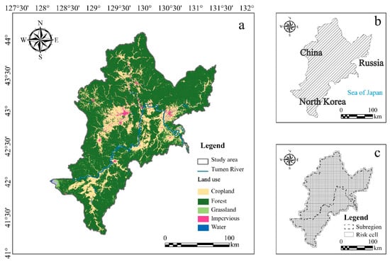
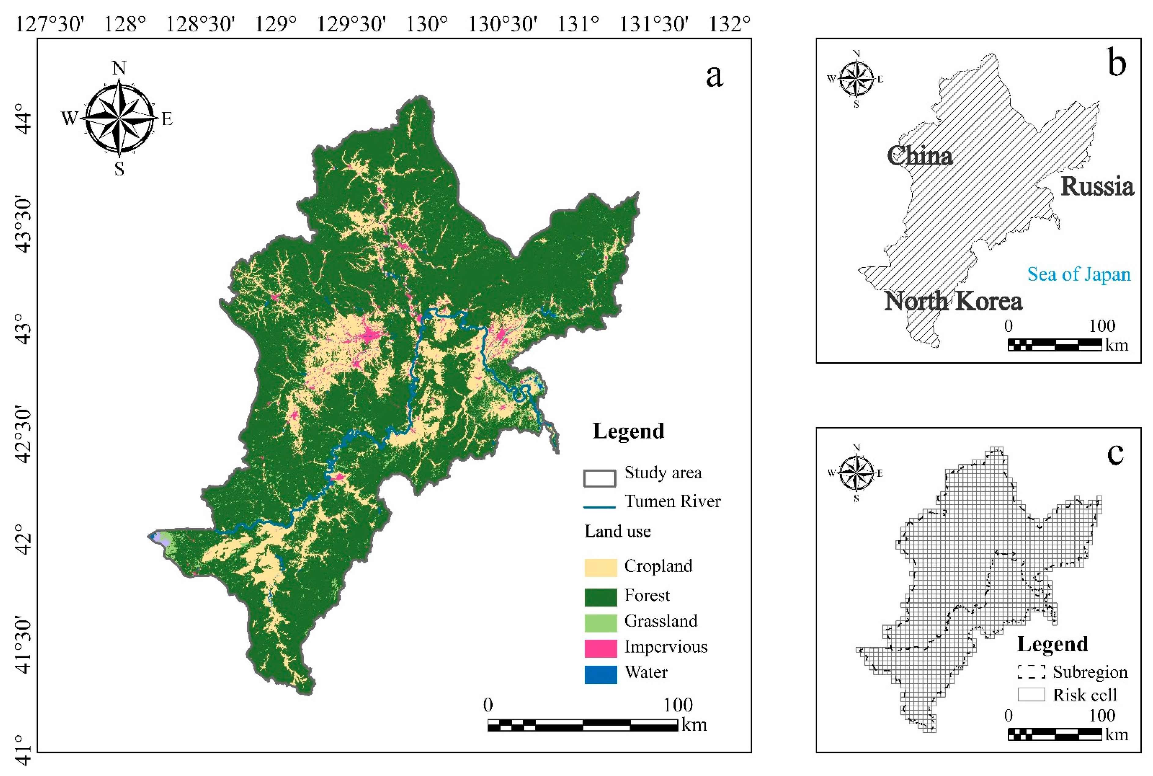
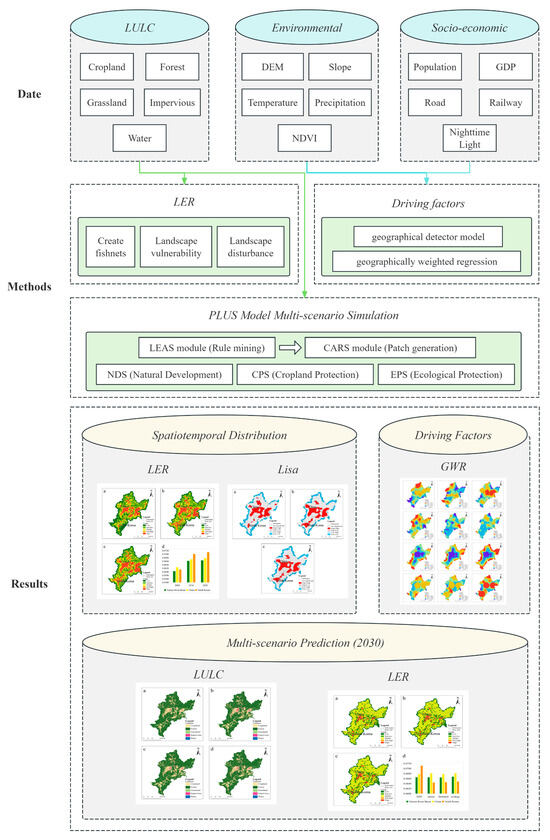
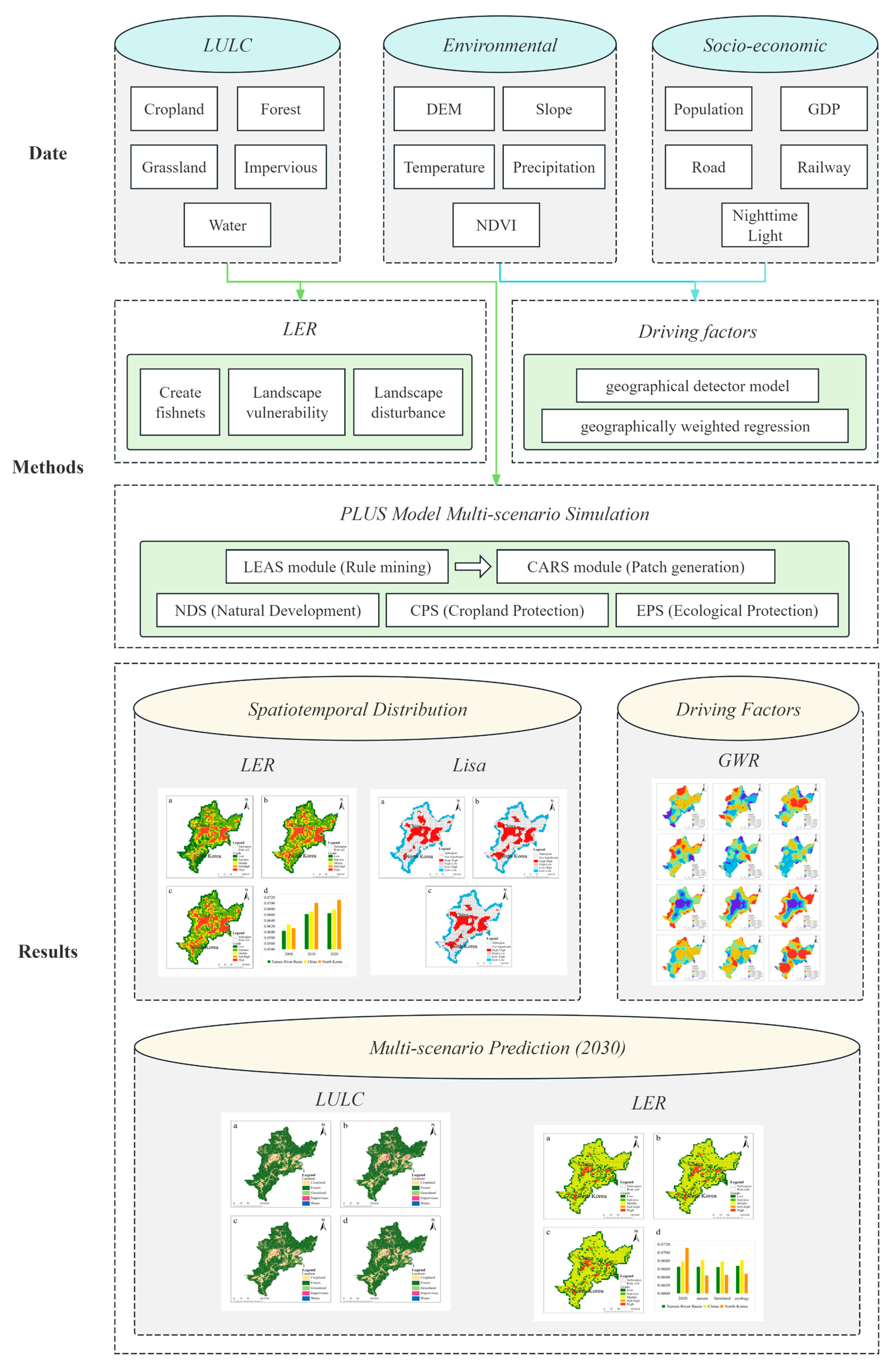
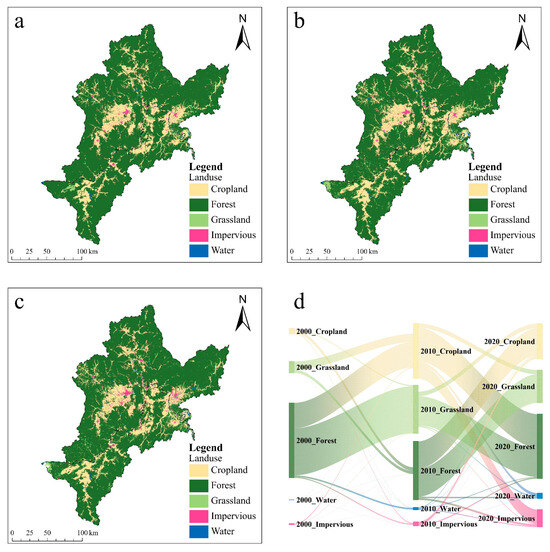
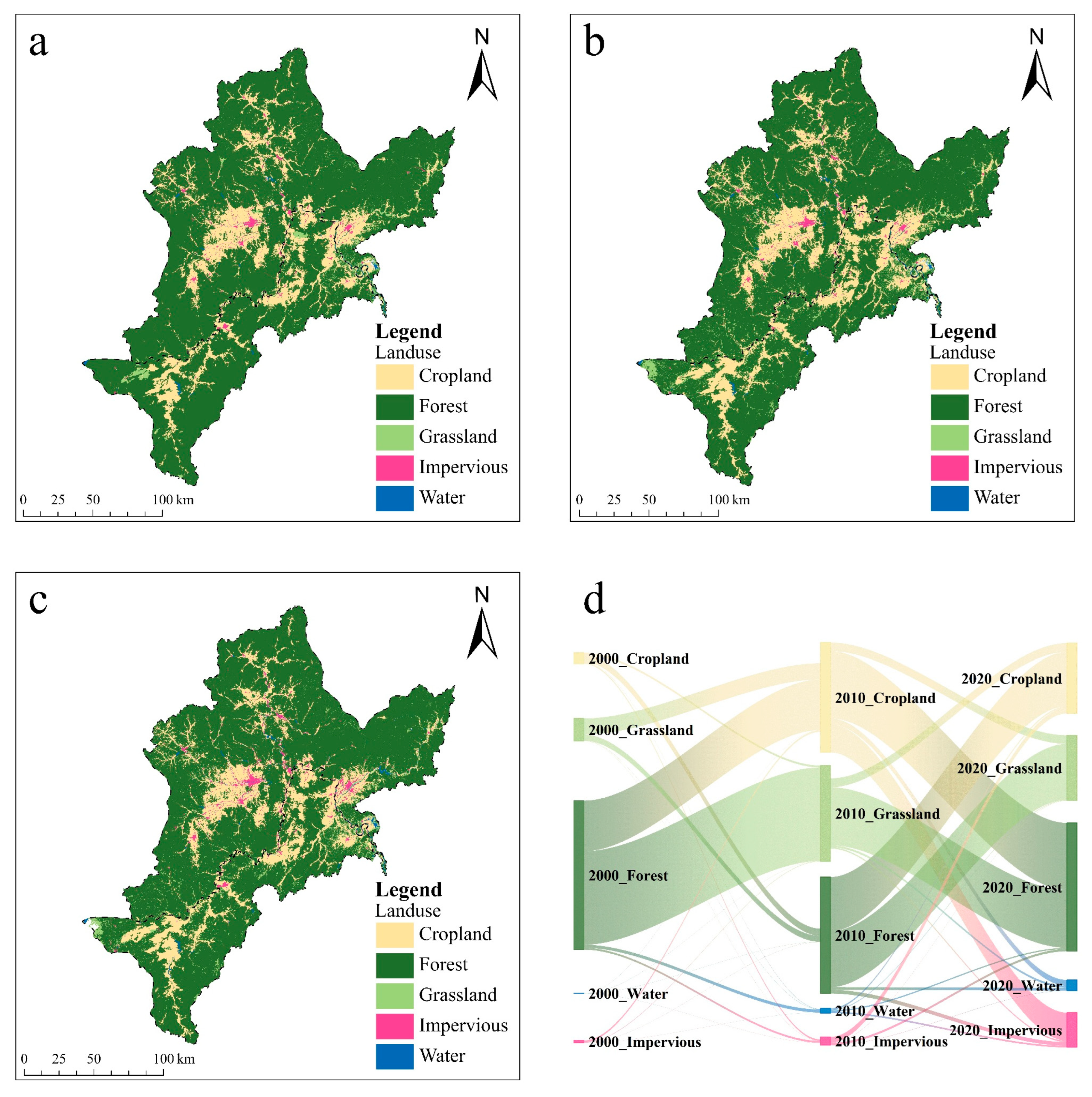
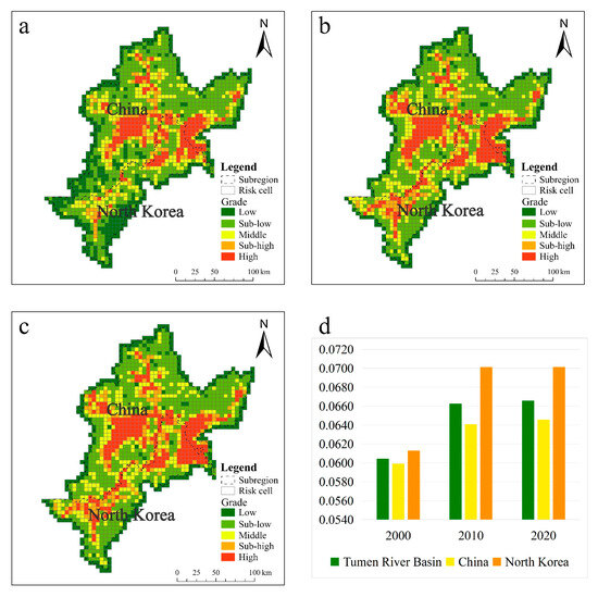
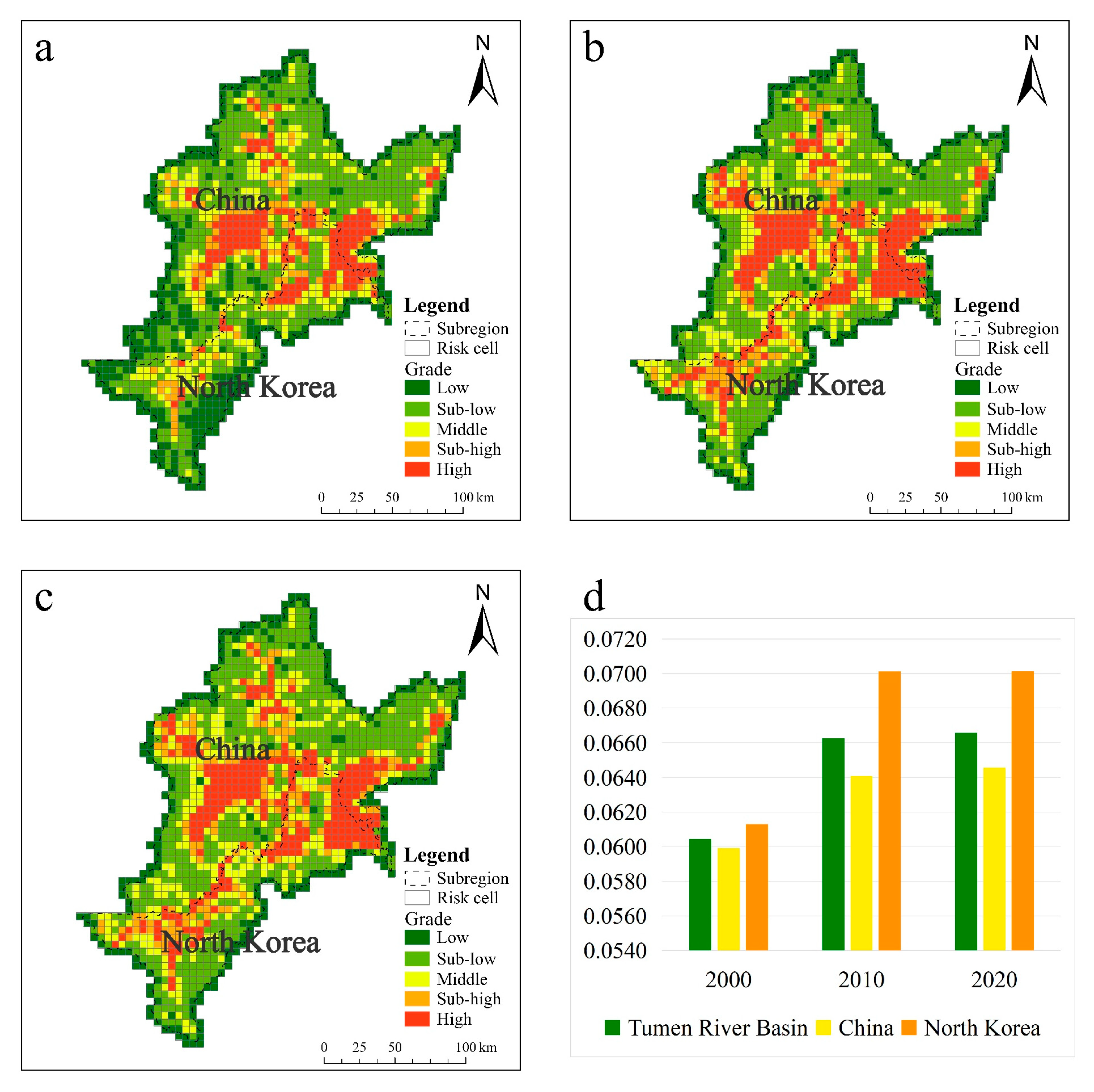
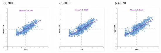
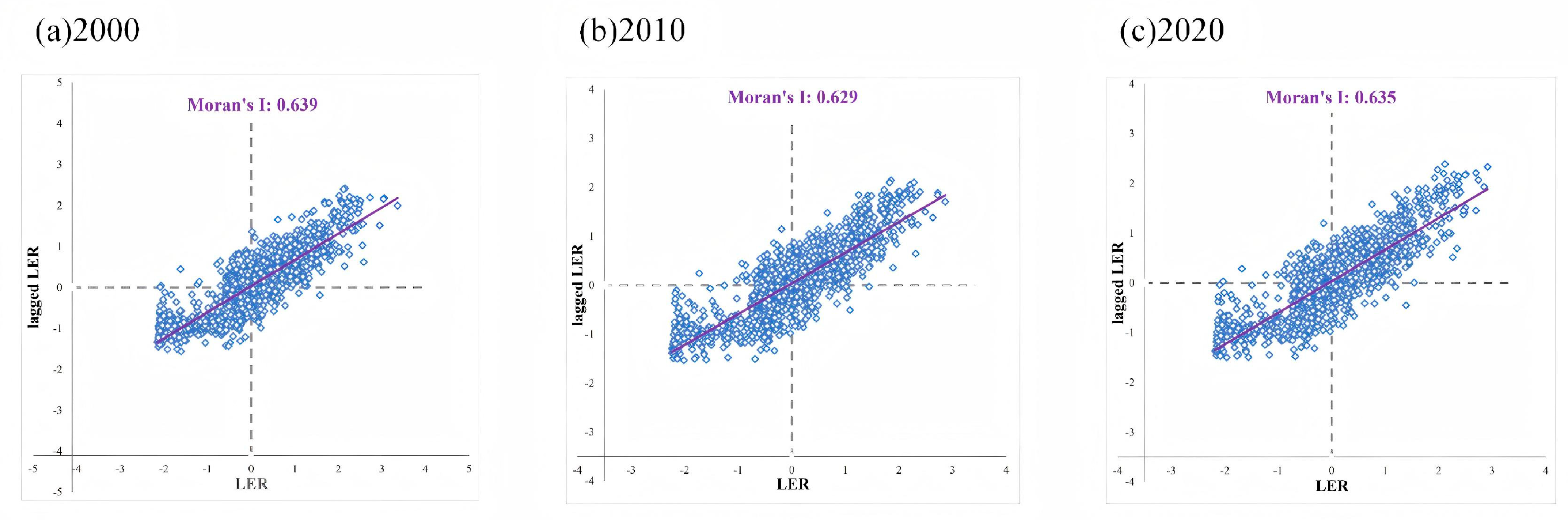
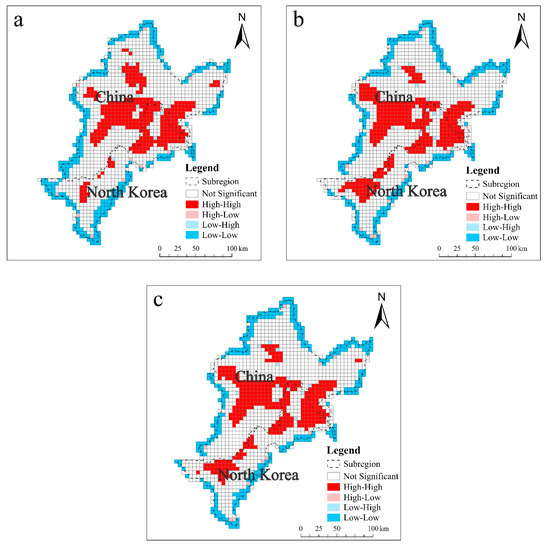
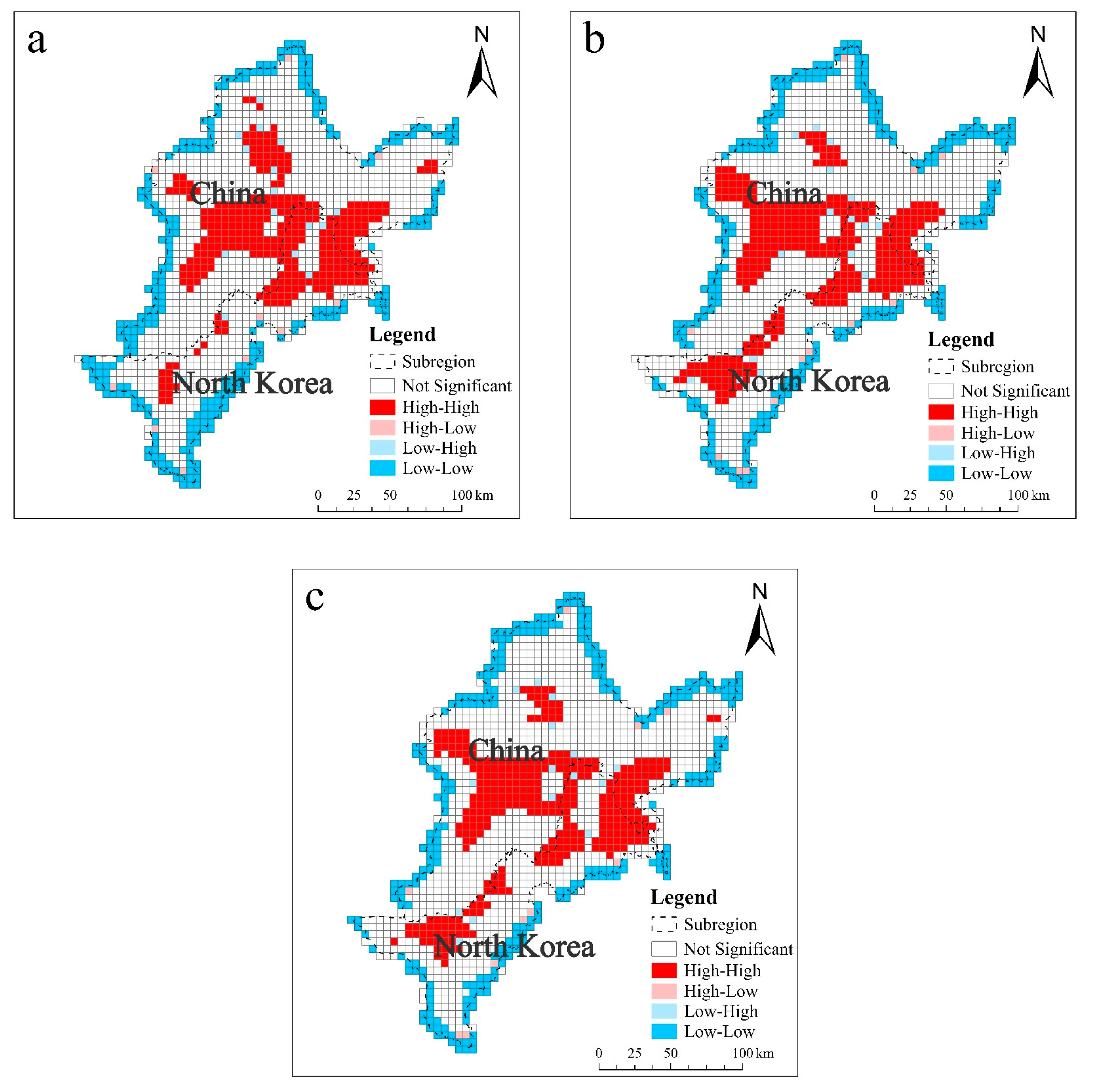
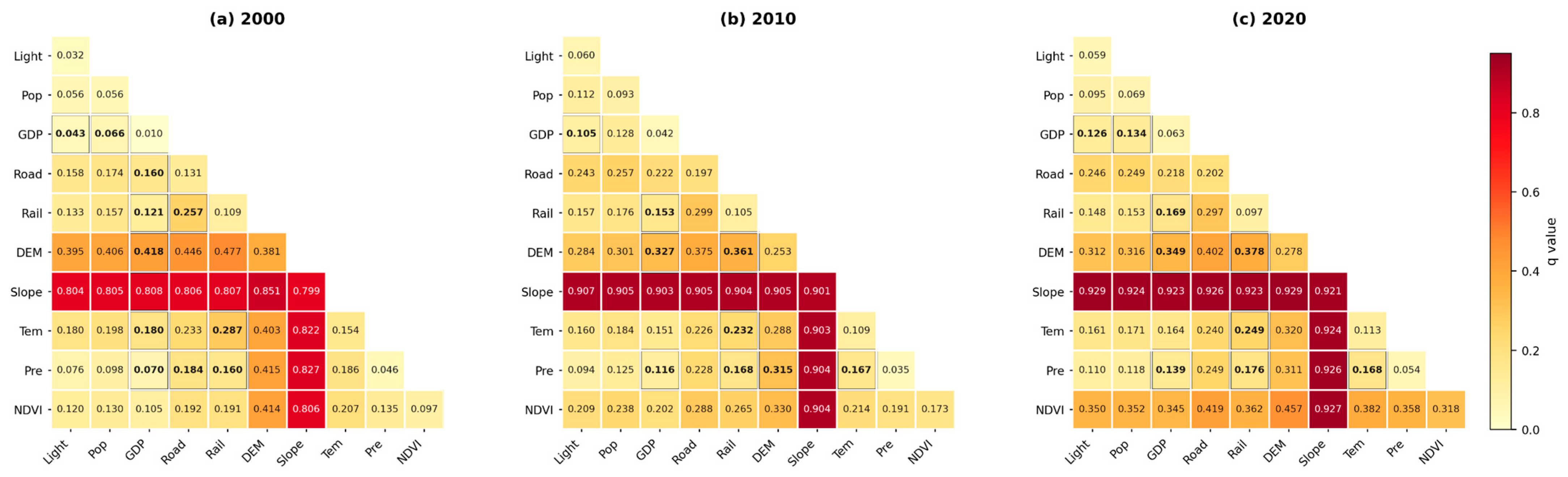
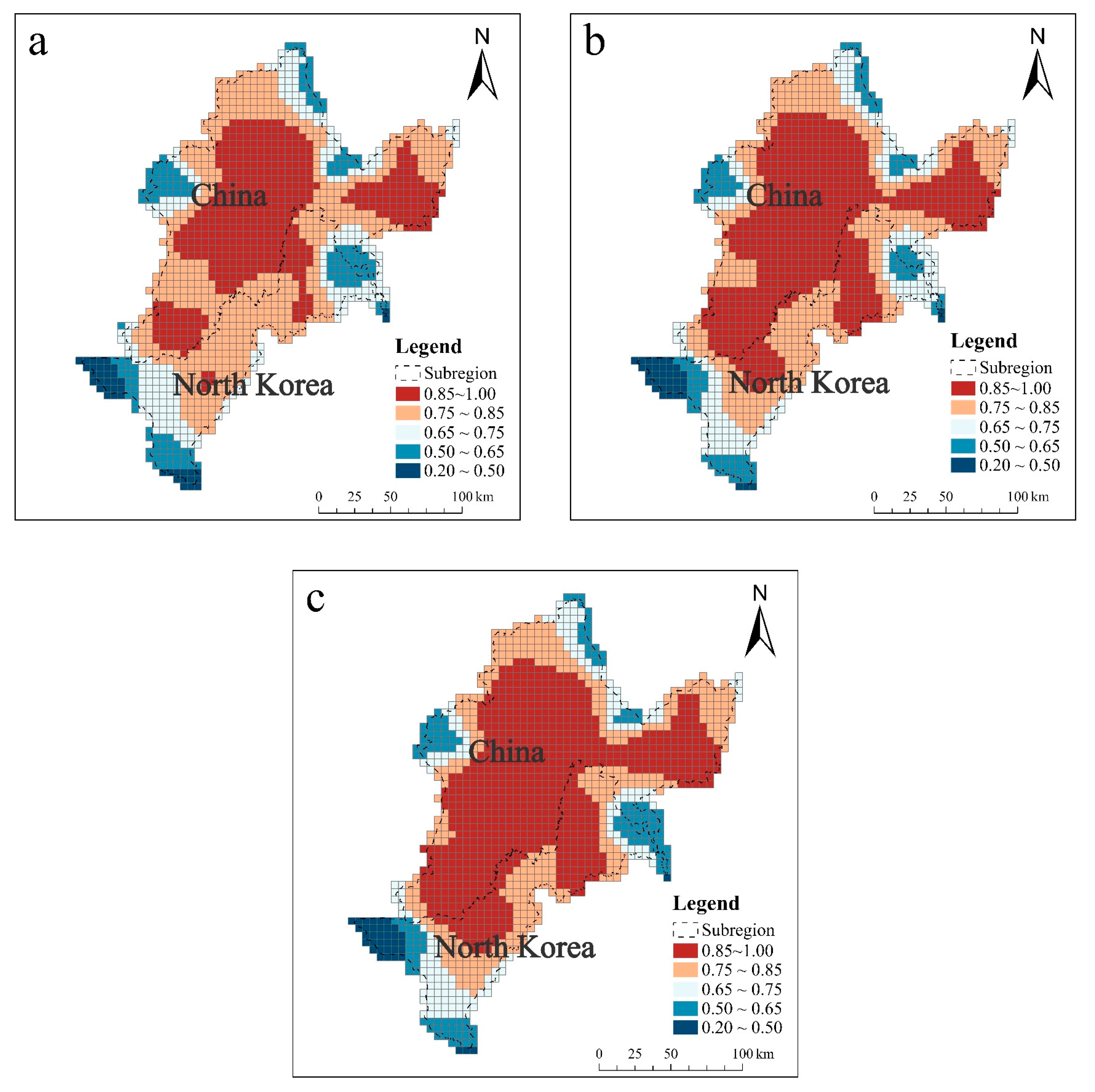
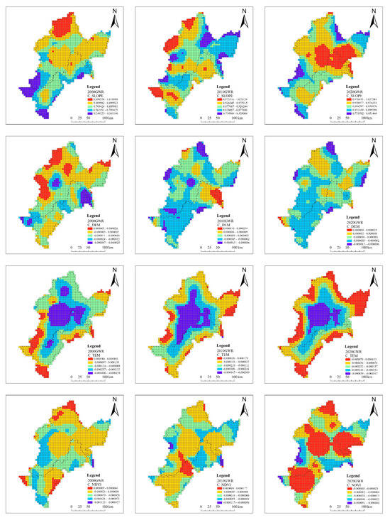
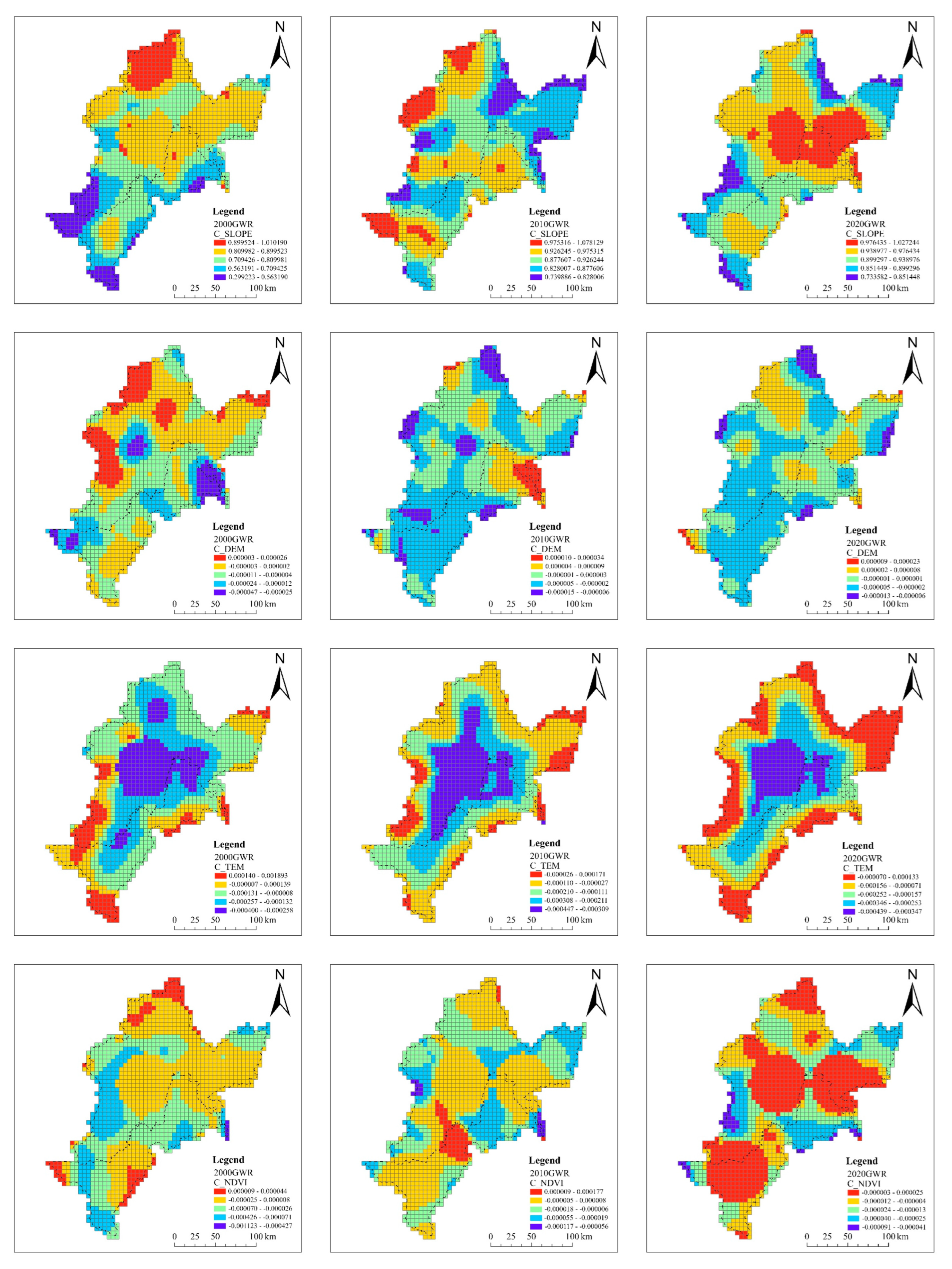
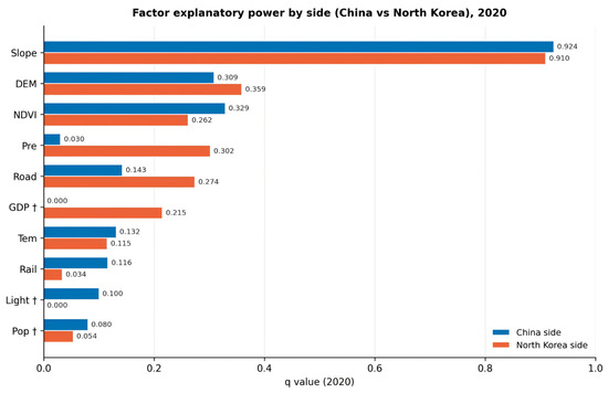
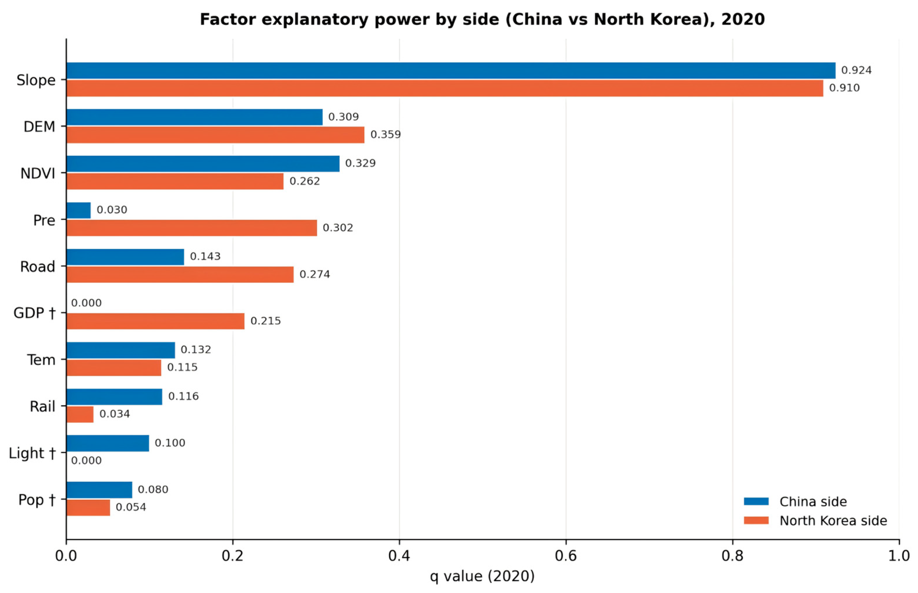
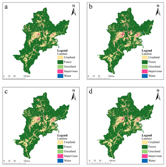
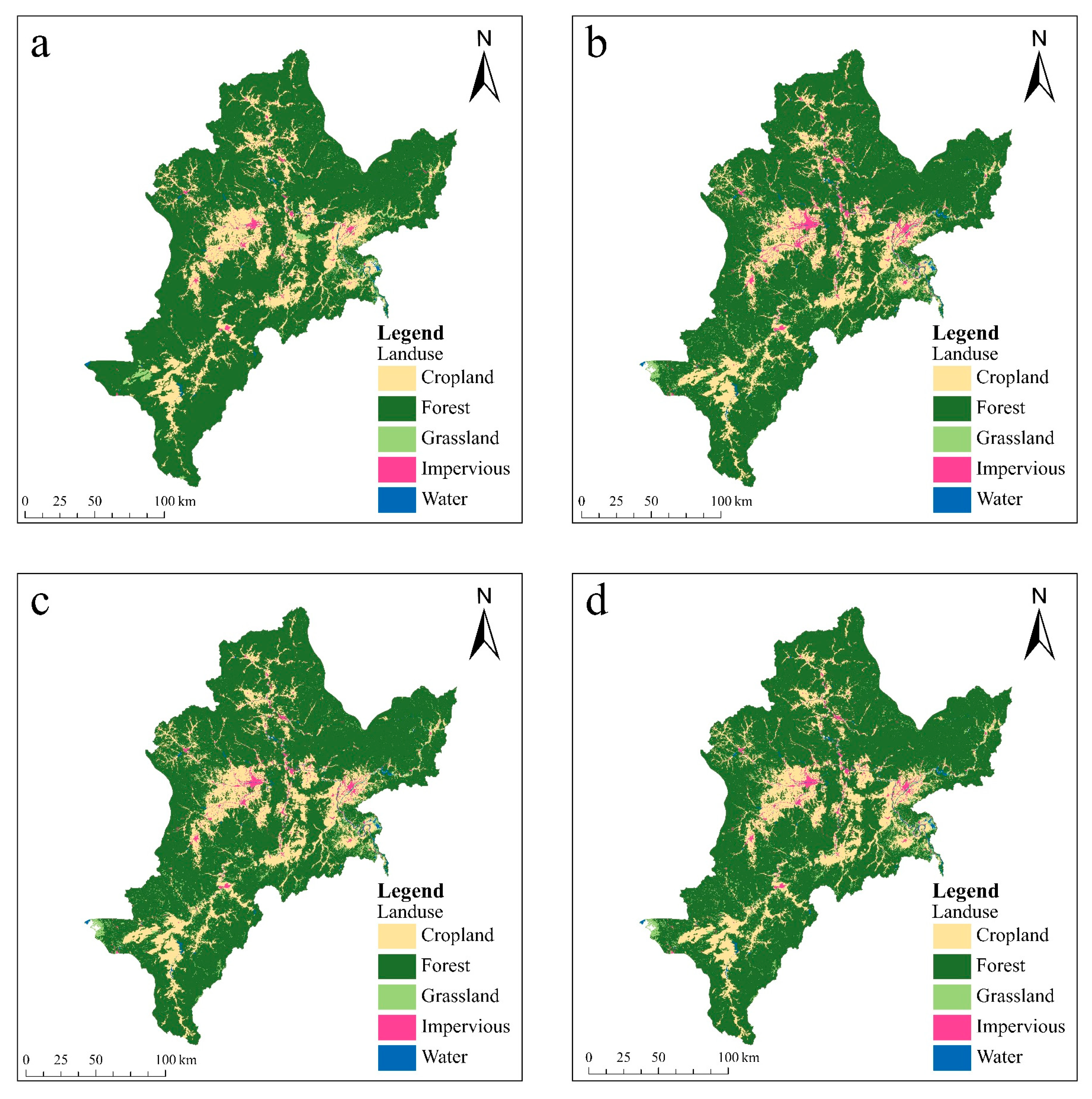
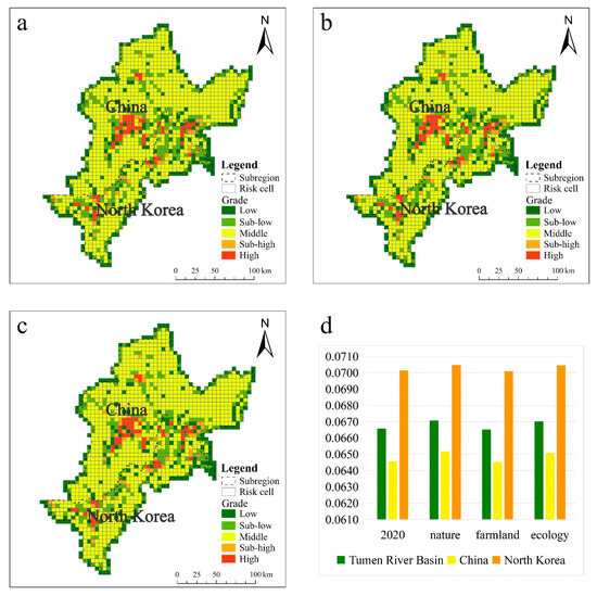
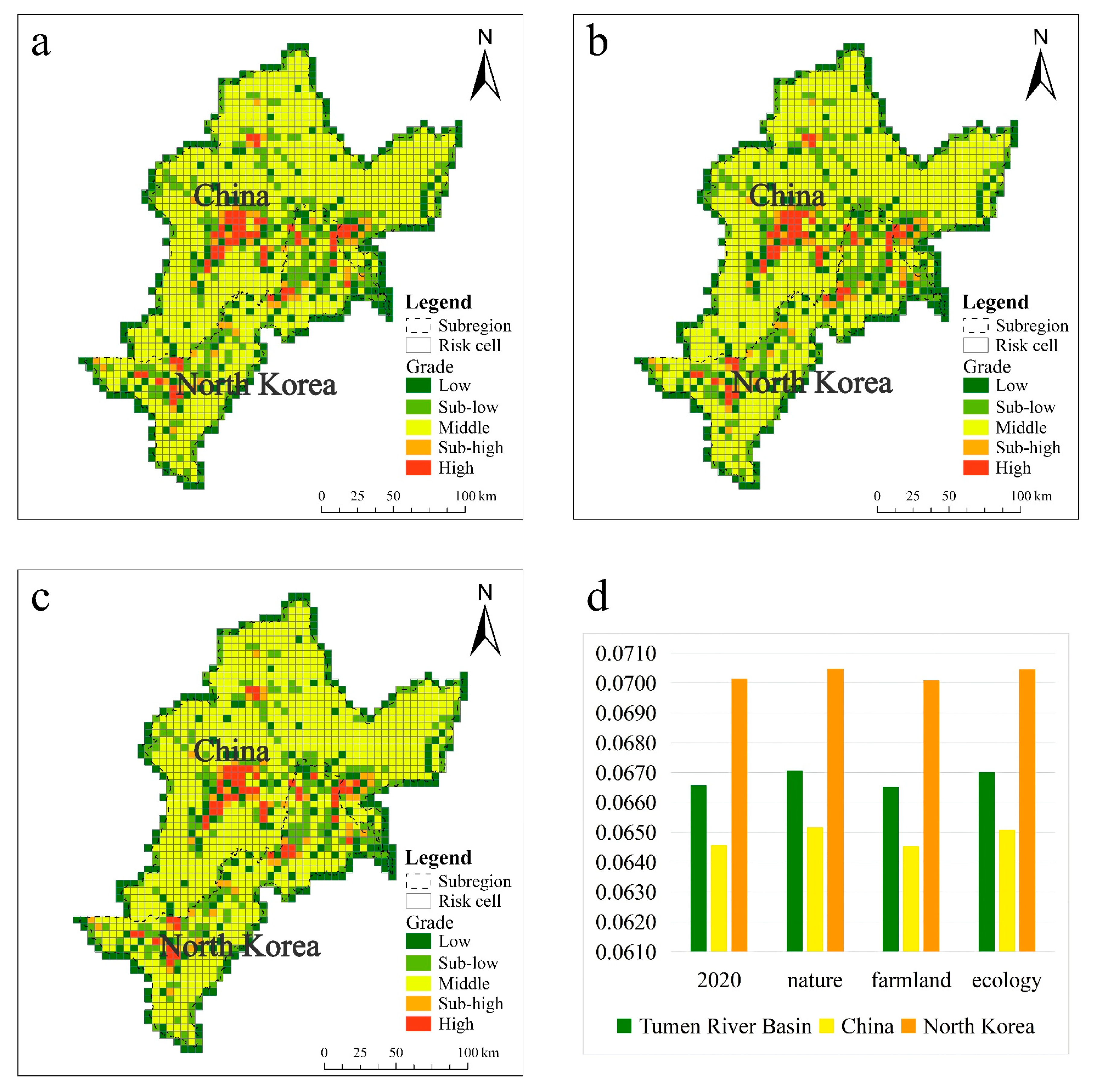

Disclaimer/Publisher’s Note: The statements, opinions and data contained in all publications are solely those of the individual author(s) and contributor(s) and not of MDPI and/or the editor(s). MDPI and/or the editor(s) disclaim responsibility for any injury to people or property resulting from any ideas, methods, instructions or products referred to in the content. |
© 2026 by the authors. Licensee MDPI, Basel, Switzerland. This article is an open access article distributed under the terms and conditions of the Creative Commons Attribution (CC BY) license.