


Highlights
What are the main findings?
- A prior-guided structural representation framework, termed PSRNet, is developed for remote sensing road segmentation to jointly exploit line-structure priors, multiscale semantic features, and frequency-domain detail cues. A learnable line-structure prior is extracted from the input image and progressively encoded to provide explicit geometric guidance for road feature learning.
- The framework introduces Local Detail Alignment (LDA) and Structure–Semantic Alignment (SSA) to interactively integrate structural priors with shallow and deep semantic features, respectively. A Frequency Detail-Aware Enhancement (FDAE) module further strengthens boundary- and fragmentation-sensitive responses, while a deep-to-shallow progressive decoder restores road connectivity and fine boundary details.
What are the implications of the main findings?
- The proposed framework provides an effective approach for extracting elongated and topologically continuous road structures from complex remote sensing scenes. The coordinated modeling of structural guidance, semantic representation, and frequencysensitive details improves the discrimination of narrow roads, weak boundaries, and locally interrupted road segments.
- PSRNet integrates structure-aware prior interaction, frequency-domain feature refinement, and progressive multiscale decoding within a unified segmentation framework, providing a practical paradigm for fine-grained extraction of road structure in remote sensing imagery.
Abstract
Roads in remote sensing imagery often contain narrow branches, complex boundaries, and long-range connections. Background interference and repeated downsampling make these structures difficult to preserve. To address these challenges, we propose a Progressive Structure Recovery Network (PSRNet) for remote sensing road segmentation. The network integrates structural-prior guidance, frequency-domain enhancement, and multiscale decoding. A line-structure prior is generated from the input image and encoded alongside hierarchical image features. Local Detail Alignment integrates prior cues with shallow features to enhance local structural details. Structure–Semantic Alignment combines deep semantic features with structural cues to refine unreliable prior responses. At the bottleneck, a Frequency Detail-Aware Enhancement module adaptively modulates the amplitude spectrum of the aligned features while preserving phase information. The reconstructed features are combined with spatial representations through residual fusion. A deep-to-shallow progressive decoder then restores spatial details and generates multiscale side predictions, which are fused to produce the final segmentation map. Experiments on the Massachusetts Roads, DeepGlobe, and CHN6-CUG datasets demonstrate the effectiveness of PSRNet for road segmentation. Ablation studies further support the complementary contributions of structural-prior guidance, frequency-domain enhancement, and progressive decoding.
1. Introduction
With the rapid development of Earth observation technology, high-resolution remote sensing imagery has become an indispensable data source for critical applications including urban planning, transportation infrastructure management, environmental monitoring, and disaster assessment [1]. These applications rely heavily on the accurate extraction of thin linear structures such as roads, rivers, power lines, and coastlines, which represent essential geographical elements that form the backbone of urban and natural systems. The precise segmentation of these thin structures serves as a fundamental prerequisite for downstream tasks including road network mapping, route planning, and geographic information analysis [2,3]. However, road segmentation in remote sensing imagery faces three inherent, interconnected challenges that have long limited the practical performance of automated methods:
- (1)
- Morphological complexity: Thin structures are inherently characterized by narrow geometries, complex topological patterns, and long-range connectivity. The extraction of such structures remains challenging because small segmentation errors may lead to broken connections and incomplete structural representations [4].
- (2)
- External environmental interference: Complex background textures and occlusions caused by natural and artificial objects introduce substantial ambiguity for feature extraction models, leading to incomplete structural representations and segmentation errors [5].
- (3)
- Algorithm-induced information loss: Modern deep segmentation architectures rely on repeated downsampling operations to reduce computational cost and expand receptive fields, which inevitably erode high-frequency spatial details and cause discontinuities in thin structures [6]. These architectural limitations exacerbate the first two challenges, resulting in common artifacts including broken connections, boundary blurring, and topological errors in segmentation outputs.
Collectively, these challenges make complete recovery of thin-structure geometry, particularly preserving connectivity and boundary fidelity, a challenging problem in remote sensing image analysis [7]. The development of remote sensing image segmentation methods has evolved significantly over the past decade, with three main paradigms emerging to address thin-structure extraction: Early approaches to remote sensing image analysis relied heavily on handcrafted features and shallow learning models, where manually designed descriptors were combined with traditional machine learning algorithms such as support vector machines and random forests [8]. While these methods perform well on simple, high-contrast scenes, they fail to generalize to complex, high-resolution imagery with significant spectral variability [9]. The introduction of fully convolutional networks (FCNs) [10] and the U-Net architecture [11] revolutionized the field by enabling end-to-end dense prediction. Although U-Net and its variants are widely used in remote sensing segmentation, CNN-based encoders still have limited long-range context modeling capability. Transformer-based methods such as LGIPNet [12] have shown that multi-level feature enhancement with edge-aware and dual-domain attention can improve dense prediction in optical remote sensing images. This further motivates the hierarchical Transformer encoder adopted in PSRNet. However, standard encoder–decoder architectures with skip connections still struggle with extremely thin structures, as the downsampling process destroys fine-grained spatial details before they can be effectively fused with high-level semantic information [13]. Variants including U-Net++ [14], DeepLabV3+ [15], and transformer-based segmentation models [16] have improved multi-scale feature fusion but still exhibit frequent discontinuities in long, thin structures [17].
To address the limitations of generic segmentation models, researchers have increasingly incorporated spatial structural priors to guide thin-structure extraction. These approaches can be categorized into three main streams:
- (1)
- Early deep learning-based methods directly learned structural representations from remote sensing images. Cheng et al. [18] proposed a cascaded end-to-end convolutional neural network for road detection and centerline extraction, jointly modeling road regions and structural information. Recent topology-aware methods further introduce explicit structural constraints to preserve connectivity and improve the completeness of extracted linear structures. For example, Zao et al. [19] proposed a transformer-based road graph extraction framework that incorporates topological representations to preserve the connectivity and structural organization of road networks. Meanwhile, detail-preserving frameworks [20] focus on maintaining fine spatial structures and reducing information loss during road extraction. However, complex remote sensing scenes and insufficient contextual modeling may still degrade segmentation robustness by weakening structural continuity and producing incomplete road representations [21].
- (2)
- Instead of directly using explicit structural priors, many recent methods exploit auxiliary supervision signals or connectivity-aware strategies to model structural continuity. For example, SWCARE [22] incorporates connectivity-aware refinement strategies and structural information to enhance the continuity and completeness of extracted road networks. DiResNet [23] introduces a direction-aware residual learning strategy that explicitly captures directional characteristics of road structures and enhances feature representation for complex linear objects. Topology-enhanced urban road extraction methods [24] incorporate geographic structural information to strengthen topological consistency and preserve road connectivity during segmentation. While these methods improve connectivity and structural completeness, they still rely on additional geometric constraints or auxiliary information, which may limit their generalization capability when facing diverse structural patterns and complex remote sensing environments.
- (3)
- The latest direction leverages generative models to learn structural priors directly from data. Denoising Diffusion Probabilistic Models (DDPMs) [25] provide a powerful probabilistic framework for modeling complex data distributions through iterative denoising processes. Improved DDPMs [26] further enhance diffusion efficiency and generation quality by optimizing noise scheduling and model design, while Denoising Diffusion Implicit Models (DDIMs) [27] accelerate the generation process through deterministic sampling strategies. Although diffusion-based methods demonstrate strong potential for learning structural priors, their iterative inference procedures and high computational costs remain challenging for practical remote sensing segmentation applications.
Frequency-domain representations provide complementary cues to spatial-domain features by emphasizing global structures, textures, boundaries, and fine-grained details, and have therefore been increasingly explored in hyperspectral and remote sensing image analysis [28]. For remote sensing imagery, Li et al. (2026) proposed a frequency domain-enhanced spectral–spatial fusion transformer that explicitly models high-frequency components corresponding to object boundaries [29]. FcaNet [30] introduces frequency channel attention networks by exploiting frequency-domain information for channel-wise feature selection, demonstrating the importance of frequency-aware representation learning. Fourier-Swin-Unet [31] integrates Fourier-based global representation learning with the Swin Transformer architecture to capture long-range dependencies while preserving detailed spatial information. WgANet [32] employs wavelet-guided attention mechanisms to decompose and enhance multi-scale frequency features, improving semantic segmentation performance in remote sensing images. However, existing frequency-based methods suffer from several limitations: Wide and Deep Fourier Neural Network [33] demonstrates the effectiveness of combining Fourier representations with deep feature learning, but global frequency transformations may introduce redundant information. In addition, fixed frequency processing strategies cannot adapt to highly variable structural characteristics of different scenes [34]. Furthermore, most existing approaches treat frequency domain processing as an isolated module rather than integrating it tightly with spatial prior information and multi-scale decoding. CAF-Net [35] proposes a unified framework for resolving spatial-frequency representation conflicts in multimodal remote sensing segmentation, highlighting the importance of effective interaction between spatial and frequency domains.
While significant progress has been made in both spatial-prior-based and frequency-domain-based methods, existing approaches suffer from a fundamental limitation: they typically employ these two types of information in isolation, without a unified framework to synergistically combine spatial geometric priors and frequency domain detail enhancement in a progressive, coarse-to-fine recovery pipeline. This gap prevents existing methods from fully addressing the core challenges of road segmentation, leaving a critical need for an integrated approach that progressively recovers structural information from rough positioning to detailed refinement.
Our work is motivated by three key insights that address the identified limitations of existing approaches:
- (1)
- Imperfect structural priors provide powerful “attention guidance” even when incomplete. Thin structures possess extremely strong geometric regularities. Even a noisy, incomplete line structure prior extracted from the input image provides a powerful “skeletal attention” mechanism that directs the model’s focus to candidate structural regions, effectively suppressing complex background interference [36]. The key is not to obtain a perfect prior, but to design mechanisms that can dynamically align and refine the imperfect prior with image features at different network depths [37].
- (2)
- Structural defects manifest as characteristic frequency signatures that can be adaptively modulated. The most common segmentation errors for thin structures—boundary blurring, local discontinuities, and width variations—are difficult to model directly in the spatial domain, and dedicated spatial-frequency detail enhancement networks for remote sensing segmentation have demonstrated that these artifacts correspond to discriminative high-frequency spectral components [38]. By adaptively modulating these frequency components, we can perform targeted “detail repair” without altering the correctly segmented structural regions, as validated by evolutionary adaptive frequency modulation restoration pipelines [39]. This frequency domain “surgical” approach provides a more precise mechanism for fixing structural defects compared to spatial domain convolution operations.
- (3)
- Progressive recovery mimics human visual understanding of linear structures. When humans identify thin structures in imagery, we follow a consistent cognitive process: first identifying the approximate location and overall topology of the structure (coarse), then refining local details and repairing broken connections (medium), and finally delineating precise boundaries (fine) [40]. This progressive reasoning process can be embedded into network design, where spatial priors provide the initial coarse localization, frequency domain processing enhances mid-level structural details, and progressive decoding recovers the final fine-grained segmentation.
Building on these insights, We propose PSRNet, a progressive structure recovery framework for remote sensing road segmentation that integrates structural-prior guidance, frequency-domain enhancement, and multiscale decoding. The core philosophy is to explicitly model the “From Prior to Frequency” recovery process, where structural information flows from the prior domain through frequency domain refinement to final spatial domain segmentation, with progressive enhancement at each stage.
To implement this progressive recovery paradigm, we introduce the Progressive Structure Recovery Network (PSRNet), a three-stage architecture specifically designed for remote sensing road segmentation. The name PSRNet encapsulates both its function (Progressive Structure Recovery) and its technical core (Prior, Structure, and Recovery).
Stage 1: Prior-Guided Interactive Encoder The first stage employs a dual-branch parallel encoder that processes both the input image and extracted line-structure prior simultaneously. Two key alignment modules enable effective use of the prior information:
- Local Detail Alignment (LDA) module: Operating at shallow network layers, LDA adaptively aligns low-level image features with structural prior features using a gating mechanism conditioned on image and prior features. This module enhances features corresponding to object boundaries, fine branches, and weak-response regions by injecting geometric information from the prior into image feature space [41].
- Structure–Semantic Alignment (SSA) module: At deeper network layers, SSA integrates high-level semantic context with structural cues to refine unreliable prior responses. By using semantic information to filter the prior, this module effectively suppresses interference from non-target linear patterns while preserving genuine structural signals [42].
Stage 2: Frequency Detail-Aware Enhancement (FDAE) Module At the network bottleneck, the FDAE module takes the structure–semantic aligned high-level representation from the encoder and transforms it into the frequency domain using the fast Fourier transform. The module adaptively modulates frequency components associated with object contours, structural variations, and local discontinuities using a learned frequency attention mask. After the inverse Fourier transformation, the enhanced frequency domain features are fused with spatial domain features through a residual connection, producing structurally discriminative high-level representations with enhanced boundary and connectivity information [43].
Stage 3: Deep-to-Shallow Progressive Decoder The final stage employs a coarse-to-fine progressive decoder that reconstructs the segmentation output through multi-level side predictions. Starting from the deepest semantic features, the decoder progressively integrates intermediate connectivity information and local boundary details at each upsampling step. Cross-scale fusion of features from different decoder levels ensures that both global topological consistency and local boundary precision are preserved in the final segmentation map [44].
This three-stage architecture creates a coherent pipeline where structural guidance is continuously refined from the initial prior input, through frequency domain enhancement, to the final progressive decoding, effectively addressing all three core challenges of road segmentation. The main contributions of this work are summarized as follows:
- We propose PSRNet, the first unified road segmentation framework that integrates spatial prior guidance, frequency domain modeling, and multi-scale progressive decoding into a cohesive “From Prior to Frequency” pipeline. This paradigm explicitly addresses the geometric recovery of thin structures, fundamentally improving structural completeness, boundary fidelity, and connectivity preservation.
- Two innovative alignment modules for prior utilization: The Local Detail Alignment (LDA) and Structure–Semantic Alignment (SSA) modules enable effective, robust use of imperfect structural priors. By dynamically aligning prior information with image features at different semantic levels, these modules simultaneously enhance weak structural responses and suppress non-target interference.
- Adaptive frequency domain enhancement mechanism: The proposed Frequency Detail-Aware Enhancement (FDAE) module provides a principled way to model and enhance structural details in the frequency domain. By adaptively modulating frequency components corresponding to structural defects, this module effectively resolves the boundary blurring and discontinuity issues common in existing methods.
- Comprehensive experimental validation: Extensive experiments on multiple public remote sensing thin-structure datasets (including Massachusetts Roads, DeepGlobe, and CHN6-CUG) demonstrate that PSRNet achieves state-of-the-art performance across multiple evaluation metrics, with particularly significant improvements in connectivity-related metrics such as Connectivity IoU and F1-score for long, thin structures.
The remainder of this paper is organized as follows: Section 2 presents the materials and methods, including the overall architecture of PSRNet and its core components. Section 3 presents the experimental results, including the datasets, experimental settings, quantitative and qualitative comparisons, and ablation studies. Section 4 discusses the model complexity and limitations of the proposed method. Finally, Section 5 concludes the paper.
2. Materials and Methods
To address the incomplete extraction of fine branches, inaccurate boundary localization, and local structural discontinuities in remote sensing road segmentation, we propose a progressive structure recovery network termed PSRNet. The proposed framework follows a hierarchical encoder–decoder architecture and establishes a sequential processing pathway from structural-prior guidance to frequency-domain feature enhancement and progressive spatial reconstruction. Specifically, PSRNet consists of three principal components: a Prior-Guided Interactive Encoder, a Frequency Detail-Aware Enhancement module, and a Deep-to-Shallow Progressive Structure Recovery Decoder. This section first introduces the overall architecture and subsequently describes each component in detail.
2.1. Overall Structure
As illustrated in Figure 1, given an input remote sensing image , a SegFormer-B3 backbone is first employed to extract four-stage hierarchical image representations:
where . The channel dimensions of the four stages are configured as , and their spatial resolutions are , respectively.
Figure 1.
Overall architecture of the proposed PSRNet.
In parallel with the image branch, a line-structure prior is generated from the input image by integrating grayscale intensity, Sobel gradient magnitude, and Laplacian responses. The resulting prior map is subsequently processed by a lightweight hierarchical prior encoder to produce multi-scale structural-prior features:
where each prior feature is aligned with its corresponding image feature in terms of channel dimension and spatial resolution.
At the shallow stages, the first- and second-stage image features are calibrated using the corresponding prior features through Local Detail Alignment modules, thereby enhancing weak responses, fine branches, and local boundary details. At the deepest stage, a Structure–Semantic Alignment module performs bidirectional interaction between the high-level image features and prior features. This process introduces structural cues into the semantic representation while using high-level semantics to rectify unreliable prior responses.
The aligned bottleneck feature is then processed by the Frequency Detail-Aware Enhancement module, which adaptively modulates its amplitude spectrum while preserving phase information. Finally, the enhanced representation is passed to a four-stage progressive decoder. The decoder gradually restores spatial resolution and generates multi-scale side predictions, which are fused to obtain the final segmentation result.
2.2. Prior-Guided Interactive Encoder
Thin structures generally occupy only a small proportion of remote sensing imagery and frequently exhibit low contrast, narrow widths, weak boundaries, and local occlusions. Although hierarchical image encoders can extract strong semantic representations, repeated downsampling may progressively attenuate weak linear responses and fine structural details.
To alleviate this limitation, a line-structure prior is introduced as auxiliary structural guidance. Rather than directly concatenating the prior map with the input image, the proposed encoder constructs two parallel hierarchical branches and performs stage-specific interaction between image and prior representations. Shallow interaction emphasizes local structural details, whereas deep interaction introduces semantic constraints to suppress unreliable prior responses.
2.2.1. Line-Structure Prior Generation and Hierarchical Encoding
The structural prior is generated by jointly modeling image intensity, first-order gradients, and second-order differential responses. Since the input image is normalized before being fed into the network, it is first restored to an intensity range close to . The grayscale representation is calculated as
where , and denote the red, green, and blue channels, respectively. The horizontal and vertical Sobel operators are applied to extract first-order gradient responses:
where * denotes convolution, are the horizontal and vertical Sobel kernels, and is a small constant introduced for numerical stability. A Laplacian operator is further employed to capture second-order intensity transitions and local structural variations:
where denotes the Laplacian kernel.
The grayscale, Sobel, and Laplacian responses are independently normalized and concatenated along the channel dimension. A learnable fusion function then generates a single-channel line-structure prior:
where denotes channel-wise concatenation, denotes sample-wise min–max normalization, denotes Group Normalization, denotes the GELU activation function, and denotes the Sigmoid function. The generated prior satisfies
It should be noted that is not regarded as a segmentation prediction. Instead, it represents a soft structural response that highlights candidate elongated structures, boundaries, centerlines, and local intensity transitions. Because Sobel and Laplacian operators respond to local intensity variations rather than road semantics, the resulting prior may contain spurious edges or miss weak road structures under noisy or low-contrast conditions. Therefore, it is used as an auxiliary cue whose contribution is adaptively modulated through subsequent feature interactions, rather than as a hard constraint. The prior map is subsequently fed into a four-stage convolutional encoder. The first stage uses a convolution with a stride of 4, while the remaining stages use convolutions with a stride of 2. Each stage also contains a feature-refinement block. The resulting prior features are aligned to the corresponding image features through bilinear interpolation:
where denotes the i-th prior encoding stage and denotes resolution alignment. Therefore, , allowing direct interaction between the image and prior features.
2.2.2. Local Detail Alignment
Shallow image features retain relatively accurate spatial details but are sensitive to background textures and appearance variations. In contrast, structural-prior features can highlight weak linear responses but may also contain irrelevant edges caused by building contours, shadows, field ridges, and other non-target objects. Therefore, directly adding the prior feature to the image representation may introduce structural noise.
To selectively incorporate reliable structural information, the Local Detail Alignment module is applied at the first two encoding stages. For the specific structure, refer to Figure 2. Let denote the image feature and corresponding prior feature. The prior feature is first projected into the image feature space using a convolution . The projected prior and the image feature are concatenated along the channel dimension:
A channel- and position-dependent gate-weight map is generated from their joint representation:
where . The gate estimates the reliability of the structural prior at each channel and spatial location. Responses with high gate values are retained, whereas potentially misleading prior responses are suppressed. The calibrated prior feature is calculated through element-wise multiplication:
where ⊙ denotes element-wise multiplication. The calibrated prior and the original image feature are concatenated again:
The concatenated representation is then processed by a feature-refinement function:
where the convolution maps the feature dimension from back to and denotes the learned feature correction. Finally, residual addition is used to preserve the original image representation:
The image-conditioned gate provides a learnable mechanism for attenuating unreliable prior responses, while the residual connection preserves the original image representation. Together, these operations allow selective incorporation of structural cues rather than unconditional fusion, although they do not guarantee complete suppression of prior errors.
Figure 2.
Architecture of the Local Detail Alignment (LDA) module. The structural prior is first projected and jointly encoded with the image feature to estimate a spatially adaptive gate map. The gated prior is then integrated with the image representation through local detail refinement, followed by residual aggregation to obtain the aligned feature.
2.2.3. Structure–Semantic Alignment
Gradient-based structural priors are not inherently class-specific. Non-target linear patterns, such as building edges, shadows, and field boundaries, may also generate strong responses. Since shallow representations contain limited semantic information, shallow gating alone cannot fully distinguish target structures from such interference.
To introduce semantic constraints into the prior representation, a Structure–Semantic Alignment module is applied at the deepest encoding stage. The specific structure is shown in Figure 3. Given , the two features are first flattened into token sequences:
where . In the prior-to-image interaction, image tokens act as queries, while prior tokens serve as keys and values:
This operation supplements the image representation with global structural information. In the opposite direction, prior tokens query the image tokens:
This interaction introduces high-level semantic constraints into the prior representation and suppresses structurally strong but semantically irrelevant responses. The bidirectional results are reshaped into two-dimensional feature maps and concatenated with the original image feature:
The resulting -channel representation is compressed and refined:
Finally, the aligned bottleneck feature is obtained through residual addition:
Unlike shallow gating, SSA incorporates high-level semantic context through bidirectional cross-attention, helping distinguish road-related structures from visually similar non-road patterns. The fused interaction features are added residually to the image features, providing a further opportunity to reduce the influence of misleading structural cues.
Figure 3.
Architecture of the Structure–Semantic Alignment (SSA) module. Deep image features and structural prior features are flattened into token sequences and interact through bidirectional cross-attention, where image tokens retrieve structural cues from the prior representation while prior tokens are semantically rectified by image features. The two cross-attended representations are then reshaped and concatenated with the original image feature, followed by convolutional fusion and residual aggregation to obtain the aligned feature .
2.3. Frequency Detail-Aware Enhancement
The deepest encoder representation contains compact semantic information but may exhibit weakened responses to narrow structures and local discontinuities. Recent frequency-domain methods, e.g., SFEET [45], have shown that frequency-selective attention and edge enhancement can strengthen weak structural and boundary responses. Inspired by this, FDAE also enhances structural details in the frequency domain, but adopts a continuous amplitude modulation strategy while preserving the phase. To refine its spectral representation before decoding, we introduce a Frequency Detail-Aware Enhancement module (FDAE) at the network bottleneck, as illustrated in Figure 4. Instead of dividing the spectrum into manually predefined frequency bands, FDAE learns a continuous, content-dependent gain map from the amplitude distribution. This formulation avoids fixed frequency thresholds and allows the spectral response of each channel and frequency coordinate to be adjusted according to the input feature.
Figure 4.
Illustration of the Frequency Detail-Aware Enhancement (FDAE) module. Given the aligned feature , its Fourier spectrum is decomposed into amplitude and phase components. The log-amplitude representation is processed by two depthwise convolution branches with different receptive fields to generate an adaptive modulation map, which selectively reweights the spectral amplitude while preserving the original phase.
Let denote the structure–semantic representation produced by the deepest encoder stage. A two-dimensional Fourier transform is independently applied to each channel:
where c denotes the channel index; and () denote the spatial and frequency coordinates, respectively; and j is the imaginary unit. The orthonormal normalization factor is consistent with the Fourier transform adopted in the implementation. The resulting complex spectrum is represented in polar form as
where denote the amplitude and phase spectra, respectively. Both components have the same dimensions as the input feature:
Because spectral amplitudes commonly exhibit a highly nonuniform numerical distribution, direct convolution on A may cause large coefficients to dominate feature learning. Therefore, logarithmic compression is applied before spectral-response modeling:
This transformation reduces the dynamic range while preserving the relative ordering of spectral magnitudes. FDAE employs two channel-wise spectral modeling branches. The first branch uses a standard depthwise convolution to capture local relationships among neighboring frequency coefficients:
where denotes depthwise convolution, represents Group Normalization, and denotes the GELU activation function. The second branch adopts a depthwise convolution with a dilation rate of 2:
Compared with the local branch, the dilation operation covers a broader neighborhood in the frequency plane without increasing the kernel size. The two branches therefore characterize spectral-amplitude dependencies at complementary receptive-field scales. Since both convolutions are depthwise, spectral patterns are first modeled independently within each feature channel, avoiding the parameter cost of dense channel coupling. The two responses are concatenated and mapped to an adaptive modulation tensor through a pointwise convolution:
where denotes channel-wise concatenation and is the Sigmoid function. The modulation tensor satisfies . The original amplitude spectrum is then reweighted as
Accordingly, the spectral gain lies within . This bounded residual modulation preserves the original amplitude as the lower bound and selectively strengthens frequency coefficients identified as informative by the two spectral branches. Unlike unconstrained spectral scaling, the formulation does not reverse or eliminate the original response, which improves the stability of frequency-domain feature learning. The phase spectrum remains unchanged during amplitude modulation, and the enhanced complex spectrum is reconstructed as
The corresponding spatial-domain representation is recovered using the inverse Fourier transform:
where extracts the real component. Retaining the original phase avoids introducing an additional phase perturbation during spectral reweighting, while the reconstructed feature reflects the learned modification of the amplitude distribution. To combine the reconstructed frequency representation with the original semantic feature, and are concatenated along the channel dimension and processed by a spatial fusion function:
The final FDAE output is obtained through residual addition:
The convolution jointly models the local correspondence between the original spatial representation and the frequency-reconstructed feature, whereas the subsequent convolution performs channel remapping. The residual pathway retains the structure–semantic representation produced by the encoder and introduces the frequency-derived correction in an additive form. Consequently, FDAE supplies the progressive decoder with a bottleneck feature that preserves the original semantic basis while incorporating adaptively enhanced spectral information.
2.4. Deep-to-Shallow Progressive Structure Recovery Decoder
The frequency-enhanced bottleneck feature obtained in Section 2.3 contains high-level semantic information and adaptively modulated spectral responses. However, the reduced spatial resolution of deep representations limits the delineation of narrow branches and fine boundaries. To recover spatial details in a hierarchical manner, we design a Deep-to-Shallow Progressive Structure Recovery Decoder. The decoder propagates the bottleneck representation through four successive stages and incorporates encoder features at the corresponding resolutions.
Let denote the encoder features supplied to the decoder, where and are generated by the Local Detail Alignment modules, , and is produced by the Structure–Semantic Alignment module. Their dimensions are written as
with
For the adopted SegFormer-B3 encoder, . At the deepest decoding stage, the FDAE output is concatenated with , and the resulting representation is processed by a decoding block:
where denotes channel-wise concatenation. The operator consists of two consecutive convolution units, each followed by Group Normalization and GELU activation. The first unit performs feature fusion and channel projection, while the second refines the resulting representation. The remaining decoding stages follow a top-down reconstruction process. At each stage, the output from the preceding deeper level is resized to the resolution of the current encoder feature and subsequently fused with it:
where denotes bilinear interpolation to and represents the corresponding decoding block. The output of each stage is expressed as . The spatial resolution is progressively recovered according to In this decoding pathway, the bottleneck information is continuously propagated toward shallower levels. Encoder features with progressively finer spatial resolutions complement the decoder representation with localization cues, enabling gradual refinement of narrow branches, structural junctions, and object boundaries. To preserve the class evidence learned at different decoding resolutions, a side-prediction head is attached to each decoder stage:
where denotes the side-output logits and K is the number of segmentation classes. The four side outputs estimate the same pixel-wise segmentation target at different spatial scales. Before fusion, they are aligned to the resolution of the shallowest side output:
where , and denotes bilinear resizing from the i-th prediction scale to the first prediction scale. The aligned logits are concatenated and aggregated through a learnable cross-scale fusion block:
where denotes GELU activation. The convolution models local correlations among predictions from different scales, and the subsequent convolution maps the fused representation to K-channel logits:
Unlike fixed summation or averaging, the learnable fusion block adaptively combines the contextual category responses provided by deeper predictions with the spatially precise responses retained by shallower predictions. The fused logits are finally resized to the original image resolution: , and . The corresponding class-probability map is obtained as
The full-resolution logits are used for the principal segmentation objective, while the side outputs provide auxiliary supervision during training. The complete loss formulation is presented in the next section.
2.5. Objective Function
The segmentation objective is designed to account for both pixel-wise classification accuracy and regional overlap. As road pixels usually occupy a considerably smaller proportion of remote sensing images than background pixels, a class-weighted cross-entropy loss is combined with Dice loss. In addition, the multi-scale side outputs introduced in Section 2.4 are incorporated into the training objective to provide supervision at different decoding resolutions.
Let denote the full-resolution logits defined in previous section, and let be the corresponding ground-truth segmentation mask. The class probability at pixel n is obtained by applying the Softmax function to :
where denotes the probability that pixel n belongs to class k. Pixels assigned the ignore label are excluded from loss computation. Let denote the set of valid pixels. To compensate for foreground-background imbalance, the class-weighted cross-entropy loss is formulated as
where is the ground-truth category of pixel n, and is the weight assigned to that category. For the binary road segmentation task, , and the class weights are set to . The larger foreground weight increases the contribution of road pixels during optimization and mitigates the dominance of the background class. Although weighted cross-entropy provides pixel-level discrimination, it does not directly characterize the spatial overlap between prediction and annotation. We therefore introduce a multi-class Dice loss. Let denote the one-hot representation of the ground-truth label. The Dice loss is defined as
where is a smoothing constant used to avoid numerical instability. In the implementation, . The summation is performed over all valid pixels in the current batch, followed by averaging over the K classes. The segmentation loss associated with a prediction is consequently written as
where and balance the two terms. Both coefficients are set to 1 in the experiments. Accordingly, the principal segmentation loss is computed from the fused prediction introduced in Section 2.4:
To constrain intermediate decoder representations, the four side-output logits defined in Equation (37) are also included in the optimization. Each side output is resized to the ground-truth resolution before loss computation:
The auxiliary objective is formulated as
where the scale-dependent weights are assigned from deep to shallow as . Larger weights are assigned to the higher-resolution side outputs because they contain more detailed spatial information and are more directly related to the final pixel-level prediction, while the deeper outputs provide complementary supervision for coarse semantic representations. The complete optimization objective is finally defined as
where . This formulation jointly optimizes the fused prediction and the intermediate decoder outputs. The weighted cross-entropy term addresses the foreground-background imbalance, the Dice term constrains region-level agreement, and the multi-scale auxiliary objective propagates segmentation supervision across the progressive decoding pathway. During inference, only the fused output is used to generate the final segmentation result; the side outputs do not introduce additional inference branches beyond those already contained in the decoder.
3. Results
To evaluate the segmentation performance of the proposed PSRNet, experiments were conducted on three representative remote sensing road datasets, namely the DeepGlobe Road Extraction Dataset, the CHN6-CUG Road Dataset, and the Massachusetts Roads Dataset. The three datasets cover substantially different geographical regions and road environments, providing complementary test scenarios for model evaluation. Quantitative comparisons with representative segmentation methods are first performed to assess the overall extraction accuracy. Ablation experiments are subsequently conducted to examine the contribution of the proposed components. In addition, qualitative comparisons and computational analyses are presented to investigate the structural reconstruction capability and efficiency of the network.
3.1. Datasets
Three publicly available road extraction datasets are employed in the experiments, namely DeepGlobe, CHN6-CUG, and the Massachusetts Roads Dataset. DeepGlobe contains satellite imagery acquired from multiple regions in South and Southeast Asia and exhibits considerable variations in road appearance and surrounding land-cover conditions. CHN6-CUG focuses on representative Chinese urban regions and includes diverse road structures under different levels of urbanization. The Massachusetts Roads Dataset consists of high-resolution aerial imagery collected over Massachusetts, USA, covering urban, suburban, and rural environments with substantial variations in road density, width, and surrounding scene composition. The differences among the three datasets in terms of geographical coverage, imaging conditions, road morphology, and background characteristics provide a comprehensive basis for evaluating the robustness and adaptability of the proposed method across heterogeneous remote sensing road scenes. A specific example is shown in Figure 5.
Figure 5.
Representative samples from the DeepGlobe, CHN6-CUG and Massachusetts road datasets, illustrating diverse road geometries, spatial scales, surrounding land-cover conditions, and scene complexities.
3.1.1. DeepGlobe Road Extraction Dataset
The DeepGlobe Road Extraction Dataset was released as part of the DeepGlobe 2018 Satellite Image Understanding Challenge. Road extraction is formulated as a binary semantic segmentation task, in which each pixel is classified as either road or background. The dataset contains 8570 RGB satellite images, including 6226 images for training, 1243 images for validation, and 1101 images for testing. Each image has a spatial size of pixels and a ground sampling distance of approximately 0.5 m/pixel. The imagery covers approximately and includes regions from India, Indonesia, and Thailand, involving urban, suburban, rural, coastal, and other land-cover environments.
The dataset contains substantial variations in road width, surface appearance, surrounding objects, and scene density. In particular, narrow roads may occupy only a limited number of pixels, while vegetation, buildings, shadows, and spectrally similar surfaces can reduce the separability between roads and their surroundings. These characteristics make DeepGlobe suitable for assessing the ability of a segmentation model to preserve fine road branches and maintain stable predictions under heterogeneous background conditions. The official validation and test annotations are not publicly accessible; therefore, the labeled training images are used to construct the training, validation, and test subsets adopted in our experiments. Since the official validation and test annotations are not publicly available, we partitioned the 6226 labeled training images into 4980 training, 622 validation, and 624 test images. Image filenames were sorted and then shuffled using a fixed split seed of 42. The validation subset was used for checkpoint selection, whereas the held-out test subset was used for final evaluation.
3.1.2. CHN6-CUG Road Dataset
The CHN6-CUG Road Dataset was introduced by Zhu et al. for very-high-resolution satellite image road extraction. The imagery was collected from Google Earth and covers six representative regions in China: Chaoyang District in Beijing, Yangpu District in Shanghai, central Wuhan, Nanshan District in Shenzhen, Sha Tin in Hong Kong, and Macao. These regions exhibit different levels of urbanization, urban morphology, and development patterns, resulting in considerable diversity in road geometry and surrounding environments.
CHN6-CUG contains 4511 manually labeled images, each with a spatial size of pixels and a spatial resolution of 0.5 m/pixel. The official partition contains 3608 training images and 903 testing images. Pixel-level annotations distinguish road regions from the background. Compared with datasets concentrated in a limited geographical domain, CHN6-CUG incorporates road scenes from multiple Chinese cities, including variations in road width, urban structure, occlusion, and surrounding land-cover patterns. These characteristics provide an additional benchmark for examining the performance of the proposed network in densely built and structurally diverse road environments.
3.1.3. Massachusetts Roads Dataset
The Massachusetts Roads Dataset was introduced by Mnih for road extraction from high-resolution aerial imagery. It contains 1171 RGB aerial images collected over Massachusetts, USA, covering a variety of urban, suburban, and rural environments. Each image has a spatial size of () pixels and covers approximately (). The dataset is officially divided into 1108 training images, 14 validation images, and 49 test images.
The corresponding annotations are binary road masks generated by rasterizing road centerlines derived from OpenStreetMap data. A line width of seven pixels is used to represent road regions without additional label smoothing. The dataset covers more than () and contains substantial variations in road density, width, orientation, and surrounding land-cover conditions. In particular, narrow roads, intersections, vegetation occlusion, and visually similar background regions introduce considerable challenges to accurate road delineation. These characteristics make the Massachusetts Roads Dataset suitable for evaluating the ability of segmentation models to preserve thin road structures and maintain spatial continuity under heterogeneous scenes.
3.2. Experimental Settings
3.2.1. Implementation Details
Experiments were conducted on a workstation equipped with two NVIDIA GeForce RTX 4090 GPUs, each with 24 GB of memory. Each training run used a single GPU. The implementation used Python 3.10.20, PyTorch 2.12.0 with CUDA 13.2, and Hugging Face Transformers 4.36.2. The MiT-B3 encoder was initialized from the publicly available checkpoint “nvidia/segformer-b3-finetuned-ade-512-512”, while the newly introduced components were initialized for road segmentation. The MiT-B3 encoder was initialized from the publicly available SegFormer-B3 pretrained model, while the newly introduced prior-guided interaction modules, Frequency Detail-Aware Enhancement module, and progressive decoder were initialized and optimized for the road segmentation task. The network performs binary semantic segmentation with background and road as the two target categories. All input RGB images and their corresponding masks were resized to pixels. Bilinear interpolation was adopted for image resizing, whereas nearest-neighbor interpolation was used for segmentation masks to avoid introducing intermediate label values. The RGB inputs were normalized using , and , which are consistent with the normalization statistics used by the pretrained backbone. Online data augmentation was applied only during training. Each training sample was randomly subjected to horizontal flipping, vertical flipping, and rotation by , , and . Random intensity perturbation was additionally introduced by adjusting the image contrast and brightness. Specifically, the contrast scaling factor was sampled from , and the brightness offset was sampled from . Each augmentation operation was independently activated with a probability of 0.5. Validation and testing samples were processed only by resizing and normalization. The network was trained for 100 epochs with a batch size of 2. AdamW was employed for parameter optimization with a weight decay of . Considering that the SegFormer encoder was initialized from pretrained parameters whereas the remaining components were newly introduced, a differential learning-rate strategy was adopted. The learning rates for the pretrained encoder and the newly added modules were set to and , respectively.
To reduce abrupt disturbance to the pretrained representation at the initial training stage, the SegFormer encoder was frozen during the first five epochs, and only the newly introduced components were optimized. From the sixth epoch onward, the encoder was unfrozen and the complete network was jointly trained using the two learning-rate groups described above. This strategy allows the task-specific modules to establish an initial adaptation to road structures before joint optimization with the pretrained backbone. The random seed was fixed to 42 for Python, NumPy, and PyTorch to improve experimental reproducibility. Model selection was based on the validation performance, and the checkpoints corresponding to the best validation IoU and F1-score were retained for subsequent evaluation. The training objective follows the formulation introduced in Section 2.5. The class weights for background and road are set to , while the coefficients of weighted cross-entropy and Dice loss are both set to 1. The overall auxiliary-loss coefficient is , and the four side predictions from deep to shallow are assigned weights of [0.1, 0.2, 0.3, 0.4]. These settings are kept consistent with the objective function defined in Section 2.5.
3.2.2. Evaluation Metrics
Road segmentation performance is evaluated using Precision, Recall, Intersection over Union (IoU), F1-score, and centerline Dice (clDice). All metrics evaluate the road foreground. Precision, Recall, IoU, and F1-score characterize pixel-level segmentation accuracy, while clDice complements these measures by assessing the agreement between road skeletons and segmentation masks.
Let and denote the numbers of true-positive, false-positive, false-negative, and true-negative pixels for the road class, respectively. Precision measures the proportion of correctly classified road pixels among all pixels predicted as road:
A higher Precision indicates that fewer background pixels are incorrectly classified as roads. Recall quantifies the proportion of correctly detected road pixels among all ground-truth road pixels:
It characterizes the capability of the model to recover road regions and is particularly sensitive to missed narrow branches. IoU measures the spatial overlap between the predicted road region and the ground-truth road region:
IoU simultaneously penalizes false-positive and false-negative predictions and is therefore used as one of the principal measures for comparing overall segmentation performance. The F1-score is the harmonic mean of Precision and Recall:
F1 provides a balanced assessment of prediction reliability and foreground coverage, making it suitable for evaluating road segmentation under pronounced foreground-background imbalance. Region-overlap metrics do not explicitly measure road connectivity. We therefore additionally report clDice as a topology-related measure of thin-structure preservation. Let M denote the predicted binary road mask, G the ground-truth mask, and the skeletonization operation. Topological precision and sensitivity are defined as:
Their harmonic mean gives
This metric evaluates how well the predicted skeleton lies within the reference road region and how completely the reference skeleton is covered by the prediction. Higher clDice indicates better centerline-based structural agreement, although it does not by itself establish that every road path is connected. All five metrics are reported as percentages, with higher values indicating better performance.
3.3. Results of Comparison Experiments
The comparison results were obtained from two sources. U-Net [11], DANet [46], ResUNet [47], LinkNet [48], DLinkNet [49], LCIRE-Net [50], SegFormer-B3 [51], CR-HR-RoadNet [52] and LOA-Net [53] were retrained and evaluated by the authors using publicly available implementations. The results for LCIRE-Net, DANet, and CR-HR-RoadNet were taken from their original publications. Since the experimental settings of the literature-reported results may differ from ours, these results serve as reference comparisons and should not be interpreted as comparisons under fully identical conditions.
3.3.1. Experiments on the DeepGlobe Road Extraction Dataset
Table 1 compares PSRNet with representative road segmentation methods on the DeepGlobe dataset. PSRNet achieves the highest reported F1-score and IoU of 80.40% and 67.23%, exceeding LOA-Net by 0.18 and 0.25 percentage points, respectively. Its Precision and Recall are 79.25% and 81.59%, respectively, while CR-HR-RoadNet achieves the highest Precision and LOA-Net the highest Recall. For structural preservation, PSRNet achieves the highest score of 87.86%, exceeding SegFormer-B3, the strongest baseline on this metric, by 3.31 percentage points. This result provides complementary evidence of improved centerline-based structural preservation. These results indicate improvements in both region overlap and centerline-based structural agreement.
Table 1.
Quantitative comparison of different methods on the DeepGlobe Road Extraction Dataset.
The qualitative results are presented in Figure 6. Three representative scenes are selected to examine the behavior of different methods in regions containing narrow branches, intersections, and locally ambiguous road structures. The red boxes highlight areas where the predictions exhibit noticeable differences. As shown in the first row, several competing methods produce incomplete responses around the narrow road segment inside the highlighted region, whereas PSRNet preserves a road structure that is closer to the reference annotation. In the second example, the road topology contains curved and intersecting structures. Some comparison methods show local interruptions or incomplete delineation within the highlighted area, while PSRNet maintains more continuous foreground responses. A similar phenomenon can be observed in the third scene, where small road branches surrounded by complex background objects are more difficult to distinguish. PSRNet retains the principal branch structure with fewer local omissions.
Figure 6.
Qualitative comparison of road segmentation results obtained by different methods on the DeepGlobe Road Extraction Dataset. (a) Input image, (b) Ground truth, (c) PSRNet, (d) U-Net, (e) DANet, (f) ResUNet, (g) LinkNet, (h) D-LinkNet, and (i) CR-HR-RoadNet.
These qualitative observations complement the IoU and clDice results, providing visual evidence of improved road-region recovery and structural preservation. The prior-guided feature interaction introduced in the encoder provides structural cues for shallow representations, while the frequency-aware bottleneck enhancement and deep-to-shallow decoding pathway further preserve and reconstruct weak road responses during feature recovery. Their individual contributions are examined separately in the ablation experiments; the results in this section reflect the overall segmentation capability of the complete network on the DeepGlobe dataset.
3.3.2. Experiments on the CHN6-CUG Road Dataset
Table 2 presents the quantitative results on the CHN6-CUG dataset. PSRNet achieves the highest reported F1-score, and IoU of 78.28%, and 64.32%, respectively. Its Recall is 80.11%, below those of LOA-Net and LCIRE-Net. PSRNet also achieves the highest clDice of 85.19%, outperforming DLinkNet by 3.05 percentage points and the SegFormer-B3 baseline by 4.75 percentage points. These results support improved preservation of road centerline structures on the CHN6-CUG dataset. These improvements support the effectiveness of PSRNet in recovering road regions while preserving their centerline structures.
Table 2.
Quantitative comparison of different methods on the CHN6-CUG dataset.
The qualitative results are shown in Figure 7. Three representative scenes are selected to further compare the segmentation characteristics of different methods on the CHN6-CUG dataset. In the first scene, the highlighted road segment is relatively narrow and its appearance is easily affected by the surrounding background. Several comparison methods exhibit local deviations or discontinuities along this segment, while PSRNet provides a more coherent prediction and better preserves the overall road geometry. In the second scene, buildings and other surrounding objects introduce stronger background interference. Some competing methods generate spurious responses or fail to recover parts of the road structures in the highlighted regions. In contrast, PSRNet suppresses these background responses more effectively and produces cleaner road predictions with clearer structural boundaries. In the third scene, the weak and narrow road segment presents a greater challenge for feature extraction, leading to partial or complete omissions in several comparison results. PSRNet still produces a stable response along this road and retains its spatial extent more faithfully.
Figure 7.
Qualitative comparison of road segmentation results obtained by different methods on the CHN6-CUG Road Dataset. (a) Input image, (b) Ground truth, (c) PSRNet, (d) U-Net, (e) DANet, (f) ResUNet, (g) LinkNet, (h) D-LinkNet, and (i) CR-HR-RoadNet.
The qualitative observations complement the improvements in IoU and clDice, suggesting better preservation of narrow road structures in complex urban backgrounds. The prior-guided feature interaction strengthens the discrimination of road structures from complex surrounding backgrounds, helping to reduce false-positive responses while retaining weak and narrow road features. Meanwhile, the frequency-aware bottleneck enhancement and deep-to-shallow progressive decoding facilitate the recovery of local details and improve the continuity of road predictions during feature reconstruction. The effectiveness of each component is further investigated in the ablation experiments; the results presented here demonstrate the overall ability of the complete PSRNet to achieve reliable and structurally coherent road segmentation on the CHN6-CUG dataset.
3.3.3. Experiments on the Massachusetts Roads Dataset
Table 3 reports the quantitative results on the Massachusetts Roads dataset. PSRNet achieves the highest reported values across all five metrics, with Precision, Recall, F1-score, IoU, and clDice reaching 78.33%, 81.48%, 79.87%, 66.87%, and 86.41%, respectively. Among the methods with reported clDice results in Table 3, PSRNet achieves the highest score of 86.41%, exceeding DLinkNet by 2.11 percentage points. Compared with the SegFormer-B3 baseline, PSRNet improves clDice by 3.35 percentage points, providing additional evidence of better centerline-based structural preservation. The improvements in both region overlap and clDice provide complementary evidence of more accurate road extraction and better centerline-based structural preservation.
Table 3.
Quantitative comparison of different methods on the Massachusetts Roads Dataset.
The qualitative results are shown in Figure 8. Three representative scenes are selected to evaluate the performance of different methods under complex backgrounds, dense road networks, and narrow road structures. In the first scene, several competing methods produce incomplete or false responses in the highlighted region, whereas PSRNet preserves the main road structure more reliably. In the second scene, which contains a dense and complex road network, PSRNet maintains more continuous road predictions and better local connectivity. In the third scene, some methods exhibit local omissions for narrow and weak-response roads, while PSRNet preserves these structures more completely and produces predictions closer to the ground-truth annotations.
Figure 8.
Qualitative comparison of road segmentation results obtained by different methods on the Massachusetts Roads Dataset. (a) Input image, (b) Ground truth, (c) PSRNet, (d) U-Net, (e) DANet, (f) ResUNet, (g) LinkNet, (h) D-LinkNet, and (i) CR-HR-RoadNet.
These qualitative observations are consistent with the region-based evaluation and the higher clDice, supporting improved recovery of narrow roads and preservation of their structural continuity. The prior-guided feature interaction enhances the representation of weak and narrow road structures, while the frequency-aware bottleneck enhancement and deep-to-shallow progressive decoding further preserve local details and connectivity during feature recovery. Overall, PSRNet demonstrates robust and balanced road segmentation performance on the Massachusetts Roads Dataset.
3.3.4. Qualitative Analysis of Challenging Scenarios
Figure 9 compares PSRNet with the SegFormer-B3 baseline in challenging scenes involving dense vegetation, complex building backgrounds, and local shadows. In the first example, both methods preserve the narrow curved road and its connection to the main road. In the second example, PSRNet produces smoother road boundaries and suppresses an isolated false-positive region visible in the baseline prediction. In the third example, both methods recover the main road, while PSRNet better preserves the narrow background gap within the road region, although this gap remains partially closed. These examples suggest improved local structural fidelity over the baseline, while highlighting remaining limitations in fine-detail recovery.
Figure 9.
Qualitative comparison in challenging road segmentation scenarios. From left to right: input image, ground-truth mask, PSRNet prediction, and SegFormer-B3 baseline prediction. From top to bottom: a narrow curved road in a densely vegetated area, a complex urban intersection, and an urban road with local shadows.
3.4. Ablation Experiments
We conduct ablation studies on the CHN6-CUG dataset to evaluate the main components, prior–feature interaction modules, and structural-prior inputs. IoU, F1-score, and clDice are used to assess segmentation accuracy and structural preservation.
Table 4 presents the contributions of the structural-prior branch with LDA and SSA (P), FDAE (F), and the progressive decoder (D). Adding P, F, or D individually improves IoU over the baseline by 2.00, 3.96, and 1.32 percentage points, respectively. FDAE provides the largest individual IoU gain, while all three components improve clDice. Two-component combinations further improve IoU and clDice over their corresponding single-component variants. Among these combinations, F + D achieves the highest IoU and clDice, reaching 63.41% and 84.53%, respectively. The full PSRNet achieves an IoU of 64.32% and a clDice of 85.19%, exceeding the baseline by 7.97 and 5.10 percentage points. These results support the complementary contributions of structural-prior guidance, frequency-domain enhancement, and progressive decoding.
Table 4.
Ablation study of the main components on the CHN6-CUG dataset. P denotes the structural-prior branch with LDA and SSA, F denotes FDAE, and D denotes the progressive decoder. Without D, the baseline decoder is retained.
The upper block of Table 5 evaluates LDA and SSA while retaining FDAE, the progressive decoder, and all structural-prior inputs. Removing LDA reduces IoU and clDice to 63.23% and 84.50%, representing decreases of 1.09 and 0.69 percentage points relative to the full model. Removing SSA yields an IoU of 63.54% and a clDice of 84.62%, corresponding to decreases of 0.78 and 0.57 percentage points. Retaining both modules achieves the best results among these variants, suggesting that shallow detail alignment and deep structure–semantic alignment provide complementary benefits for integrating structural priors with image features. The lower block of Table 5 compares different structural-prior inputs with both LDA and SSA retained. Grayscale + Sobel achieves an IoU of 62.98% and a clDice of 84.14%, while Grayscale + Laplacian achieves 63.27% and 84.56%, respectively. Combining all three inputs increases IoU to 64.32% and clDice to 85.19%. Relative to Grayscale + Sobel and Grayscale + Laplacian, the full combination improves IoU by 1.34 and 1.05 percentage points and clDice by 1.05 and 0.63 percentage points, respectively. These results suggest that Sobel and Laplacian responses provide complementary structural cues when combined with grayscale information.
Table 5.
Fine-grained ablation study on the CHN6-CUG dataset. FDAE and the progressive decoder are retained in all configurations. The upper block evaluates LDA and SSA with all prior inputs retained. The lower block evaluates prior input components with both LDA and SSA retained.
3.5. Sensitivity Analysis of Loss Weights
We investigate the sensitivity of PSRNet to the loss weights on the CHN6-CUG dataset. As shown in Table 6, each experiment varies one weight while keeping the others at their default values: CE = 1.0, Dice = 1.0, and aux = 0.4. The CE and Dice weights are individually adjusted to 0.5 and 1.5, while the auxiliary supervision weight is adjusted to 0.2 and 0.6.
Table 6.
Sensitivity analysis of loss weights on the CHN6-CUG dataset. Each variant changes one weight while keeping the others at their default values. The default configuration is , , and .
The default configuration achieves the highest reported IoU and clDice, reaching 64.32% and 85.19%, respectively. Adjusting the CE weight reduces IoU by 0.96–1.20 percentage points, while changing the Dice weight leads to decreases of 1.23–1.30 percentage points. Varying the auxiliary supervision weight produces smaller IoU decreases of 0.72–1.04 percentage points. Across all tested configurations, clDice ranges from 84.53% to 85.19%, with a maximum difference of 0.66 percentage points. These results indicate that segmentation performance varies moderately within the tested weight ranges, while centerline-based structural preservation remains relatively stable. The default weights provide the best observed balance between region overlap and structural preservation among the evaluated configurations.
4. Discussion
4.1. Model Complexity and Time Complexity Analysis
Table 7 compares the model complexity of PSRNet with several representative road segmentation methods in terms of the number of parameters and floating-point operations (FLOPs). PSRNet contains 71.89 M parameters, which is higher than ResNet, CR-HR-RoadNet, LinkNet, U-Net, DANet, and LCIRE-Net, but substantially lower than the 217.65 M parameters of D-LinkNet. The relatively large parameter size mainly results from the use of the MiT-B3 backbone together with the additional prior-guided feature interaction and progressive feature recovery components. Therefore, although PSRNet improves the representation of structural and frequency information, this improvement is accompanied by an increase in model storage and parameter complexity. In contrast to its parameter count, PSRNet requires only 57.23 GFLOPs for an input image, which is the lowest computational cost among all compared methods in Table 7. For example, the computational costs of LinkNet, LCIRE-Net, and D-LinkNet are 109.68, 106.09, and 120.31 GFLOPs, respectively, while DANet and ResNet require more than 300 GFLOPs. This characteristic is closely related to the architectural design of PSRNet. The structure–semantic interaction is mainly performed at the deepest encoder stage with a relatively low spatial resolution, while the frequency enhancement module employs depthwise operations to process spectral responses. In addition, the progressive decoder gradually recovers spatial details through multi-stage feature fusion rather than maintaining high-dimensional representations at the original image resolution. These designs constrain the computational overhead introduced by the additional modules.
Table 7.
Comparison of model complexity in terms of parameters and GFLOPs.
Overall, PSRNet exhibits a trade-off between parameter complexity and computational cost. Although its parameter size remains relatively large, the substantially reduced FLOPs indicate that the proposed structural and frequency enhancement mechanisms do not introduce excessive spatial computation. Nevertheless, the increased number of parameters may still limit its deployment on memory-constrained edge devices, suggesting that model compression and lightweight architectural design remain important directions for further improvement.
4.2. Limitations
Despite the performance gains achieved by PSRNet, several limitations remain to be addressed. One concern lies in the model scale. Although the proposed architecture maintains relatively low computational complexity, PSRNet still contains 71.89 M parameters owing to the MiT-B3 backbone and the additional feature interaction modules. The resulting storage and memory requirements may restrict its deployment on resource-constrained platforms. Future work could therefore explore lighter hierarchical encoders, parameter-efficient interaction mechanisms, or model compression strategies to reduce the overall model footprint while preserving segmentation accuracy. Another limitation concerns the reliance of structural-prior generation on conventional gradient-based operators. The fixed Sobel and Laplacian kernels capture local intensity variations but lack semantic discrimination. Consequently, they may respond strongly to building boundaries, field edges, shadows, and textured backgrounds, while producing weak or fragmented responses for low-contrast or occluded roads. Their fixed local filtering patterns also limit adaptation to variations in road width and image resolution. Although PSRNet learns to fuse these responses and uses LDA and SSA to refine their interaction with image features, the underlying operators remain fixed, and unreliable prior cues may not be fully suppressed. A potential future direction is to replace or augment these handcrafted responses with a learnable prior-generation module. Such a module could predict road-specific structural cues directly from image features under segmentation supervision, allowing the prior to adapt to semantic context and spatial scale. Whether this approach improves robustness to noise, shadows, and occlusion requires further experimental validation. The current framework also remains challenged by extremely narrow roads, heavily occluded segments, and backgrounds with road-like appearances. Although structural guidance, frequency enhancement, and progressive decoding support road structure recovery, the training objective does not explicitly constrain road connectivity. In the current implementation, clDice is used only as an evaluation metric and is not incorporated into the training loss. Consequently, improved clDice scores do not imply that connectivity is explicitly optimized, and local interruptions or incorrect connections may still occur. Future work could incorporate a differentiable clDice-based loss or other topology-aware loss functions to impose explicit constraints on road connectivity alongside the existing segmentation objective. The generalization ability of PSRNet also requires broader validation. The experiments in this study are conducted on DeepGlobe, CHN6-CUG, and the Massachusetts Roads Dataset, which cover different geographical regions and road environments. However, they still cannot fully represent the variations encountered in practical remote sensing applications, such as differences in sensors, spatial resolutions, seasons, illumination conditions, and geographical domains. Evaluating the model on more diverse multi-source datasets and under cross-domain settings would therefore be valuable for assessing its robustness in real-world applications. The current evaluation is limited to road segmentation datasets. The applicability of PSRNet to other thin-structure categories, such as rivers, power lines, and coastlines, remains unverified and requires dedicated experiments.
5. Conclusions
This paper presents PSRNet, a progressive structure recovery network for remote sensing road segmentation, aiming to improve the extraction of narrow, weak, and structurally discontinuous roads in complex scenes. The proposed framework integrates structural prior guidance, frequency-aware feature enhancement, and progressive decoding into a unified architecture. By introducing structural cues into the encoder, enhancing discriminative responses in the frequency domain, and progressively recovering spatial details during decoding, PSRNet strengthens both road representation and structural reconstruction. Experiments on multiple public road extraction datasets demonstrate that PSRNet achieves consistently competitive performance under diverse geographical and scene conditions. The ablation studies further verify the effectiveness and complementarity of the proposed components, while the complexity analysis shows that the model maintains a relatively moderate computational cost despite its enhanced representation capability. Overall, PSRNet provides an effective solution for remote sensing road segmentation, particularly for scenes involving weak responses and fragmented road structures.
Future work will explore lightweight hierarchical backbones as alternatives to MiT-B3 and investigate model compression techniques, including structured pruning, knowledge distillation, and quantization. These strategies aim to reduce parameter count, memory footprint, and inference latency for deployment on resource-constrained edge devices. Their effectiveness will be assessed on target hardware, considering the trade-off between computational efficiency and the preservation of narrow road structures. Further directions include learnable structural-prior generation and topology-aware training losses to improve prior reliability and explicitly constrain road connectivity.
Author Contributions
Conceptualization, Y.C., H.S. and L.S.; methodology, Y.C.; software, H.S. and X.W.; validation, L.S. and Q.Y.; data curation, H.S.; writing—original draft preparation, Y.C., H.S., X.W. and L.S.; writing—review and editing, W.L. and L.S.; visualization, X.W. and L.S.; supervision, L.S.; funding acquisition, Y.C. and L.S. All authors have read and agreed to the published version of the manuscript.
Funding
This research was funded by the Scientific Research Innovation Capability Support Project for Young Faculty under grant SRICSPYF-BS2025007, the Central Government Guided Local Science and Technology Development Fund Projects of Qinghai Province under Grant 2026-GX-Z26, and the Basic Research Program of Jiangsu Province under grant BK20250043.
Data Availability Statement
The DeepGlobe Road Extraction dataset used in this study is publicly available from https://github.com/GeneralLi95/deepglobe_land_cover_classification_with_deeplabv3plus (accessed on 1 May 2026). The Massachusetts Roads Dataset is publicly available from the Road and Building Detection Datasets webpage maintained by Volodymyr Mnih at the University of Toronto. https://www.kaggle.com/datasets/balraj98/massachusetts-roads-dataset (accessed on 15 May 2026). The CHN6-CUG Roads Dataset is publicly available from the public dataset-sharing platform of the China University of Geosciences (Wuhan). https://github.com/CUG-URS/CHN6-CUG-Roads-Dataset (accessed on 15 May 2026). No new datasets were created in this study.
Acknowledgments
During the preparation of this manuscript, the authors used [Deep Seek, v4 pro] for the purposes of grammar check and English polishing. The authors have reviewed and edited the output and take full responsibility for the content of this publication.
Conflicts of Interest
The authors declare no conflicts of interest.
References
- Zhang, T.; Li, J.; Feng, Y.; Wen, Z.; Liu, L.; Li, J. MSMamba: A Multi-Semantic Mamba Framework for Referring Remote Sensing Image Segmentation. Remote Sens. 2026, 18, 1949. [Google Scholar] [CrossRef] [Scilit]
- Wang, X.; Liu, X.; Mahmood, A.; Yang, Y.; Li, X. LGD-DeepLabV3+: An Enhanced Framework for Remote Sensing Semantic Segmentation via Multi-Level Feature Fusion and Global Modeling. Sensors 2026, 26, 1008. [Google Scholar] [CrossRef] [Scilit] [PubMed]
- Iqbal, J.; Masood, A.; Sultani, W.; Ali, M. Leveraging Topology for Domain Adaptive Road Segmentation in Satellite and Aerial Imagery. ISPRS J. Photogramm. Remote Sens. 2023, 206, 106–117. [Google Scholar] [CrossRef] [Scilit]
- Wei, Y.; Zhang, K.; Ji, S. Simultaneous Road Surface and Centerline Extraction from Large-Scale Remote Sensing Images Using CNN-Based Segmentation and Tracing. IEEE Trans. Geosci. Remote Sens. 2020, 58, 8919–8931. [Google Scholar] [CrossRef] [Scilit]
- Yang, R.; Zhong, Y.; Liu, Y.; Lu, X.; Zhang, L. Occlusion-Aware Road Extraction Network for High-Resolution Remote Sensing Imagery. IEEE Trans. Geosci. Remote Sens. 2024, 62, 5619316. [Google Scholar] [CrossRef] [Scilit]
- Alom, M.Z.; Taha, T.M.; Yakopcic, C.; Westberg, S.; Sidike, P.; Nasrin, M.S.; Esesn, B.C.V.; Awwal, A.A.S.; Asari, V.K. The History Began from AlexNet: A Comprehensive Survey on Deep Learning Approaches. arXiv 2018, arXiv:1803.01164. [Google Scholar]
- Mnih, V.; Hinton, G.E. Learning to Detect Roads in High-Resolution Aerial Images. In Proceedings of the Computer Vision—ECCV 2010, Heraklion, Crete, Greece, 5–11 September 2010; pp. 210–223. [Google Scholar] [CrossRef] [Scilit]
- Sheykhmousa, M.; Mahdianpari, M.; Ghanbari, H.; Mohammadimanesh, F.; Ghamisi, P.; Homayouni, S. Support Vector Machine Versus Random Forest for Remote Sensing Image Classification: A Meta-Analysis and Systematic Review. IEEE J. Sel. Top. Appl. Earth Obs. Remote Sens. 2020, 13, 6308–6325. [Google Scholar] [CrossRef] [Scilit]
- Zhu, X.X.; Tuia, D.; Mou, L.; Xia, G.S.; Zhang, L.; Xu, F.; Fraundorfer, F. Deep Learning in Remote Sensing: A Comprehensive Review and List of Resources. IEEE Geosci. Remote Sens. Mag. 2017, 5, 8–36. [Google Scholar] [CrossRef] [Scilit]
- Long, J.; Shelhamer, E.; Darrell, T. Fully Convolutional Networks for Semantic Segmentation. In Proceedings of the IEEE Conference on Computer Vision and Pattern Recognition (CVPR), Boston, MA, USA, 7–12 June 2015; pp. 3431–3440. [Google Scholar] [CrossRef] [Scilit]
- Ronneberger, O.; Fischer, P.; Brox, T. U-Net: Convolutional Networks for Biomedical Image Segmentation. In Proceedings of the Medical Image Computing and Computer-Assisted Intervention—MICCAI 2015, Munich, Germany, 5–9 October 2015; pp. 234–241. [Google Scholar] [CrossRef] [Scilit]
- Sun, L.; Liu, H.; Wang, X.; Zheng, Y.; Chen, Q.; Wu, Z.; Fu, L. Local–Global Information Perception Network for Salient Object Detection in Optical Remote Sensing Images. IEEE Trans. Geosci. Remote Sens. 2025, 63, 5625518. [Google Scholar] [CrossRef] [Scilit]
- Badrinarayanan, V.; Kendall, A.; Cipolla, R. SegNet: A Deep Convolutional Encoder-Decoder Architecture for Image Segmentation. IEEE Trans. Pattern Anal. Mach. Intell. 2017, 39, 2481–2495. [Google Scholar] [CrossRef] [Scilit] [PubMed]
- Zhou, Z.; Siddiquee, M.M.R.; Tajbakhsh, N.; Liang, J. UNet++: Redesigning Skip Connections to Exploit Multiscale Features in Image Segmentation. IEEE Trans. Med. Imaging 2020, 39, 1856–1867. [Google Scholar] [CrossRef] [Scilit] [PubMed]
- Chen, L.C.; Zhu, Y.; Papandreou, G.; Schroff, F.; Adam, H. Encoder-Decoder with Atrous Separable Convolution for Semantic Image Segmentation. In Proceedings of the Computer Vision—ECCV 2018, Munich, Germany, 8–14 September 2018; pp. 833–851. [Google Scholar] [CrossRef] [Scilit]
- Dosovitskiy, A.; Beyer, L.; Kolesnikov, A.; Weissenborn, D.; Zhai, X.; Unterthiner, T.; Dehghani, M.; Minderer, M.; Heigold, G.; Gelly, S.; et al. An Image is Worth 16x16 Words: Transformers for Image Recognition at Scale. In Proceedings of the International Conference on Learning Representations (ICLR), Virtual, 3–7 May 2021. [Google Scholar]
- Zheng, S.; Lu, J.; Zhao, H.; Zhu, X.; Luo, Z.; Wang, Y.; Fu, Y.; Feng, J.; Xiang, T.; Torr, P.H.; et al. Rethinking Semantic Segmentation from a Sequence-to-Sequence Perspective with Transformers. In Proceedings of the IEEE/CVF Conference on Computer Vision and Pattern Recognition (CVPR), Nashville, TN, USA, 20–25 June 2021; pp. 6881–6890. [Google Scholar]
- Cheng, G.; Wang, Y.; Xu, S.; Wang, H.; Xiang, S.; Pan, C. Automatic Road Detection and Centerline Extraction via Cascaded End-to-End Convolutional Neural Network. IEEE Trans. Geosci. Remote Sens. 2017, 55, 3322–3337. [Google Scholar] [CrossRef] [Scilit]
- Zao, Y.; Zou, Z.; Shi, Z. Road Graph Extraction via Transformer and Topological Representation. IEEE Geosci. Remote Sens. Lett. 2024, 21, 2502205. [Google Scholar] [CrossRef] [Scilit]
- Wang, Z.; Luo, Z.; Zhu, Q.; Peng, S.; Ran, L.; Zhang, Y.; Wang, L.; Chen, Y.; Hu, Z.; Luo, J. A Road-Detail Preserving Framework for Urban Road Extraction From VHR Remote Sensing Imagery. IEEE Trans. Geosci. Remote Sens. 2025, 63, 5400913. [Google Scholar] [CrossRef] [Scilit]
- Du, Y.; Sheng, Q.; Zhang, W.; Zhu, C.; Li, J.; Wang, B. From Local Context-Aware to Non-Local: A Road Extraction Network via Guidance of Multi-Spectral Image. ISPRS J. Photogramm. Remote Sens. 2023, 203, 230–245. [Google Scholar] [CrossRef] [Scilit]
- Zhang, L.; Yuan, S.; Dong, R.; Zheng, J.; Gan, B.; Fang, D.; Liu, Y.; Fu, H. SWCARE: Switchable Learning and Connectivity-Aware Refinement Method for Multi-City and Diverse-Scenario Road Mapping Using Remote Sensing Images. Int. J. Appl. Earth Obs. Geoinf. 2024, 127, 103665. [Google Scholar] [CrossRef] [Scilit]
- Ding, L.; Bruzzone, L. DiResNet: Direction-Aware Residual Network for Road Extraction in VHR Remote Sensing Images. IEEE Trans. Geosci. Remote Sens. 2020, 59, 10243–10254. [Google Scholar] [CrossRef] [Scilit]
- Li, X.; Wang, Y.; Zhang, L.; Liu, S.; Mei, J.; Li, Y. Topology-Enhanced Urban Road Extraction via a Geographic Feature-Enhanced Network. IEEE Trans. Geosci. Remote Sens. 2020, 58, 8819–8830. [Google Scholar] [CrossRef] [Scilit]
- Ho, J.; Jain, A.; Abbeel, P. Denoising Diffusion Probabilistic Models. In Proceedings of the Advances in Neural Information Processing Systems, Virtual, 6–12 December 2020; Volume 33, pp. 6840–6851. [Google Scholar]
- Nichol, A.Q.; Dhariwal, P. Improved Denoising Diffusion Probabilistic Models. In Proceedings of the 38th International Conference on Machine Learning, PMLR, Virtual, 18–24 July 2021; Volume 139, pp. 8162–8171. [Google Scholar]
- Song, J.; Meng, C.; Ermon, S. Denoising Diffusion Implicit Models. arXiv 2022, arXiv:2010.02502. [Google Scholar]
- Wu, X.; Sun, L.; Zhang, G.; Chen, Y.; Wu, Z. MDFPF-Net: Multi-Domain Feature Perceptual Fusion Network for Hyperspectral Unmixing. IEEE Trans. Geosci. Remote Sens. 2026. early access. [Google Scholar] [CrossRef] [Scilit]
- Li, X.; Xu, F.; Li, J.; Su, Y.; Li, L.; Lyu, X.; Xu, Z.; Kaup, A. Frequency Domain-Enhanced Spectral-Spatial Fusion Transformer for Semantic Segmentation of Remote Sensing Images. Inf. Fusion 2026, 132, 104248. [Google Scholar] [CrossRef] [Scilit]
- Qin, Z.; Zhang, P.; Wu, F.; Li, X. FcaNet: Frequency Channel Attention Networks. In Proceedings of the IEEE/CVF International Conference on Computer Vision (ICCV), Montreal, QC, Canada, 10–17 October 2021; pp. 783–792. [Google Scholar]
- Zhou, J.; Shen, Z.; Cheng, H. Fourier-Swin-Unet: A Lightweight Network for Remote Sensing Image Semantic Segmentation. In Proceedings of the 2024 IEEE 6th International Conference on Civil Aviation Safety and Information Technology (ICCASIT), Hangzhou, China, 23–25 October 2024; pp. 1025–1030. [Google Scholar] [CrossRef] [Scilit]
- Wang, Y.; Cao, L.; Deng, H. WgANet: A Wavelet-Guided Attention Network for Remote Sensing Image Semantic Segmentation. IEEE J. Sel. Top. Appl. Earth Obs. Remote Sens. 2026, 19, 702–716. [Google Scholar] [CrossRef] [Scilit]
- Xi, J.; Ersoy, O.K.; Cong, M.; Zhao, C.; Qu, W.; Wu, T. Wide and Deep Fourier Neural Network for Hyperspectral Remote Sensing Image Classification. Remote Sens. 2022, 14, 2931. [Google Scholar] [CrossRef] [Scilit]
- Tan, M.; Le, Q. Efficientnetv2: Smaller Models and Faster Training. In Proceedings of the International Conference on Machine Learning, PMLR, virtually, 18–24 July 2021; pp. 10096–10106. [Google Scholar]
- Ma, M.; Wu, S.; Li, X.; Wei, H. CAF-Net: A Unified Framework for Resolving Spatial-Frequency Representation Conflicts in Multimodal Remote Sensing Segmentation. Remote Sens. 2026, 18, 2284. [Google Scholar] [CrossRef] [Scilit]
- Wang, Y.; Zhang, J.; Jiang, R.; Yang, X.; Yun, T.; Zhang, L. GeoSAM-Lite: A Lightweight Foundation Model for Onboard Remote Sensing Segmentation. arXiv 2026, arXiv:2607.03760. [Google Scholar]
- Feng, J.; Li, F.; Zhang, J.; Chen, S.; Liang, Y.; Chen, J.; Shang, R. Decouple and Rectify: Semantics-Preserving Structural Enhancement for Open-Vocabulary Remote Sensing Segmentation. arXiv 2026, arXiv:2604.02010. [Google Scholar]
- Fu, J.; Yu, Y.; Wang, L. FSDENet: A Frequency and Spatial Domains-Based Detail Enhancement Network for Remote Sensing Semantic Segmentation. IEEE J. Sel. Top. Appl. Earth Obs. Remote Sens. 2025, 18, 19378–19392. [Google Scholar] [CrossRef] [Scilit]
- Ma, J.; Hu, S.; Zhang, X.; Wan, J.; Huang, J.; Zhang, L.; Khan, S. EvoIR: Towards All-in-One Image Restoration via Evolutionary Frequency Modulation. arXiv 2025, arXiv:2512.05104. [Google Scholar]
- Palmer, S.E. Visual Perception and World Knowledge: Notes on a Model of Sensory-Cognitive Interaction. Explor. Cogn. 1975, 279–307. [Google Scholar]
- Vaswani, A.; Shazeer, N.; Parmar, N.; Uszkoreit, J.; Jones, L.; Gomez, A.N.; Kaiser, Ł.; Polosukhin, I. Attention is All you Need. Adv. Neural Inf. Process. Syst. 2017, 30, 5998–6008. [Google Scholar]
- Hu, J.; Shen, L.; Sun, G. Squeeze-and-excitation networks. In Proceedings of the IEEE Conference on Computer Vision and Pattern Recognition, Salt Lake City, UT, USA, 18–23 June 2018; pp. 7132–7141. [Google Scholar]
- Roberts, R.A.; Mullis, C.T. Digital Signal Processing; Addison-Wesley Longman Publishing Co., Inc.: Boston, MA, USA, 1987. [Google Scholar]
- Chen, L.C.; Papandreou, G.; Schroff, F.; Adam, H. Rethinking Atrous Convolution for Semantic image Segmentation. arXiv 2017, arXiv:1706.05587. [Google Scholar]
- Sun, L.; Shi, B.; Zheng, Y.; Xiao, L.; Cao, Y. SFIEET: Spectral Frequency-Induced Edge Enhancement Transformer for Hyperspectral Change Detection. IEEE Trans. Geosci. Remote Sens. 2026, 64, 5501515. [Google Scholar] [CrossRef] [Scilit]
- Fu, J.; Liu, J.; Tian, H.; Li, Y.; Bao, Y.; Fang, Z.; Lu, H. Dual attention network for scene segmentation. In Proceedings of the 2019 IEEE/CVF Conference on Computer Vision and Pattern Recognition (CVPR), Long Beach, CA, USA, 15–20 June 2019; pp. 3141–3149. [Google Scholar]
- Xiao, X.; Lian, S.; Luo, Z.; Li, S. Weighted res-unet for high-quality retina vessel segmentation. In Proceedings of the 2018 9th International Conference on Information Technology in Medicine and Education (ITME), Hangzhou, China, 19–21 October 2018; pp. 327–331. [Google Scholar]
- Chaurasia, A.; Culurciello, E. Linknet: Exploiting encoder representations for efficient semantic segmentation. In Proceedings of the 2017 IEEE Visual Communications and Image Processing (VCIP), St. Petersburg, FL, USA, 10–13 December 2017; pp. 1–4. [Google Scholar]
- Zhou, L.; Zhang, C.; Wu, M. D-LinkNet: LinkNet with pretrained encoder and dilated convolution for high resolution satellite imagery road extraction. In Proceedings of the 2018 IEEE/CVF Conference on Computer Vision and Pattern Recognition Workshops (CVPRW), Salt Lake City, UT, USA, 18–22 June 2018; pp. 192–1924. [Google Scholar]
- Duan, Y.; Yang, D.; Qu, X.; Zhang, L.; Chao, L.; Gan, P.; Yuan, S.; Qin, H.; Qu, J. Lcire-net: Lightweight cross-modal information interaction for road feature extraction from remote sensing images and gps trajectory/lidar. IEEE Trans. Geosci. Remote Sens. 2024, 63, 2000418. [Google Scholar] [CrossRef] [Scilit]
- Xie, E.; Wang, W.; Yu, Z.; Anandkumar, A.; Alvarez, J.M.; Luo, P. SegFormer: Simple and efficient design for semantic segmentation with transformers. Adv. Neural Inf. Process. Syst. 2021, 34, 12077–12090. [Google Scholar]
- Chen, J.; Yang, L.; Wang, H.; Zhu, J.; Sun, G.; Dai, X.; Deng, M.; Shi, Y. Road extraction from high-resolution remote sensing images via local and global context reasoning. Remote Sens. 2023, 15, 4177. [Google Scholar] [CrossRef] [Scilit]
- Huang, B.; Lu, Y.; Li, Z.; Yang, R.; Shi, Y.; Gu, Z.; Zhong, Y. LOA-Net: Lightweight Orientation-Aware Network for Road Extraction from Remote Sensing Imagery. Remote Sens. 2026, 18, 2716. [Google Scholar] [CrossRef] [Scilit]
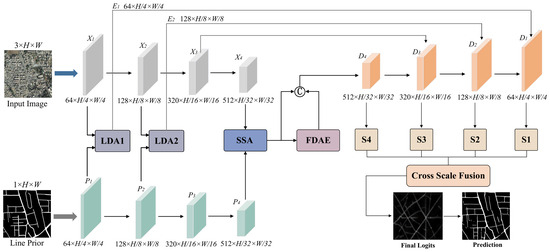
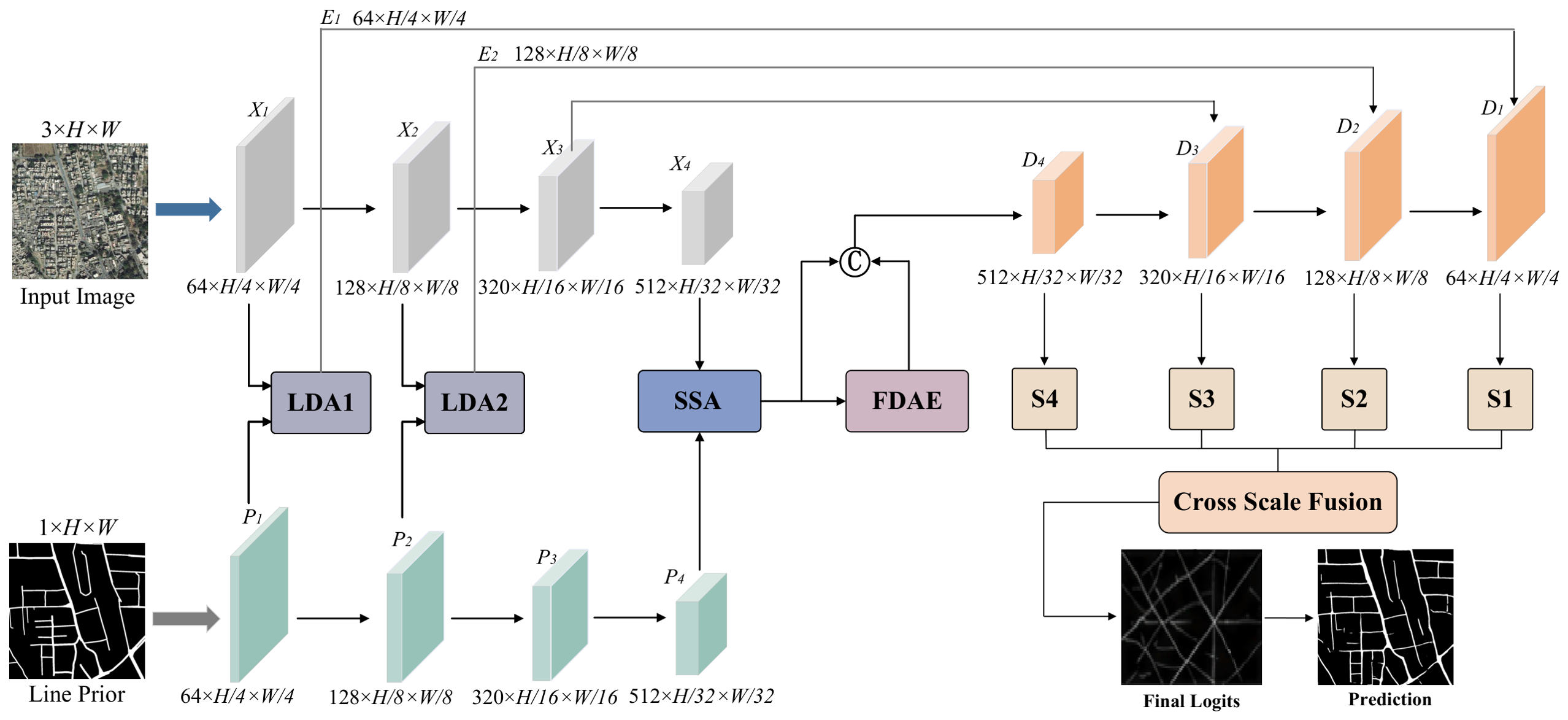
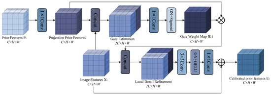
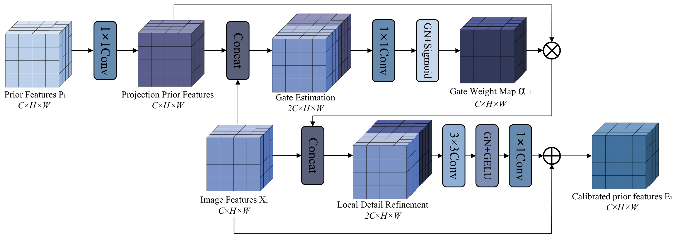
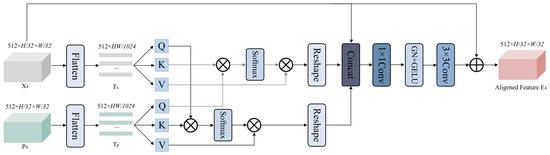
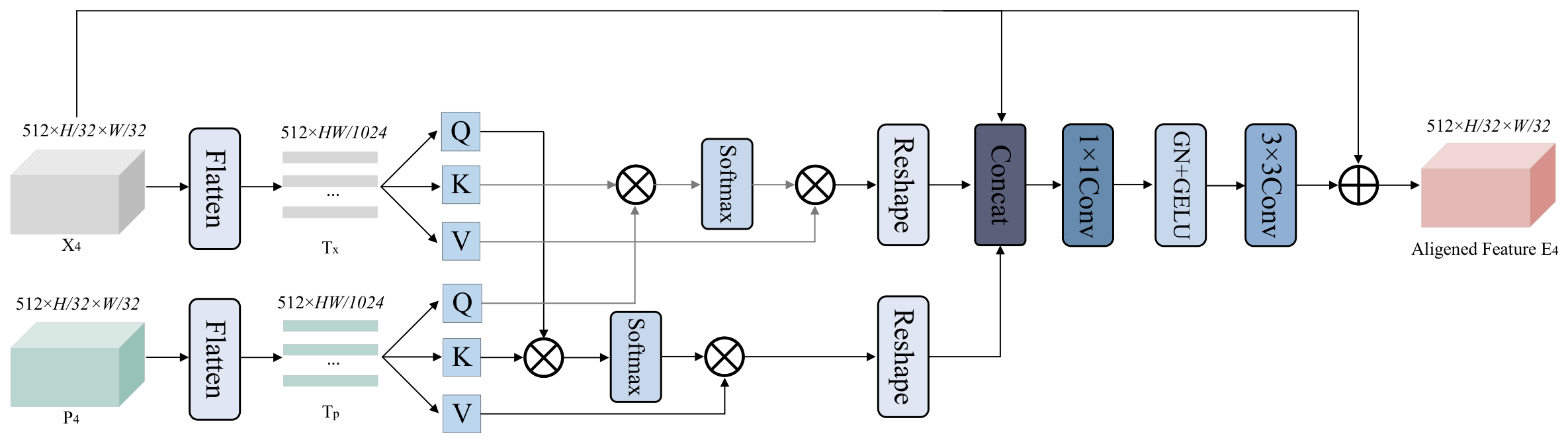
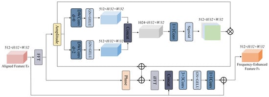
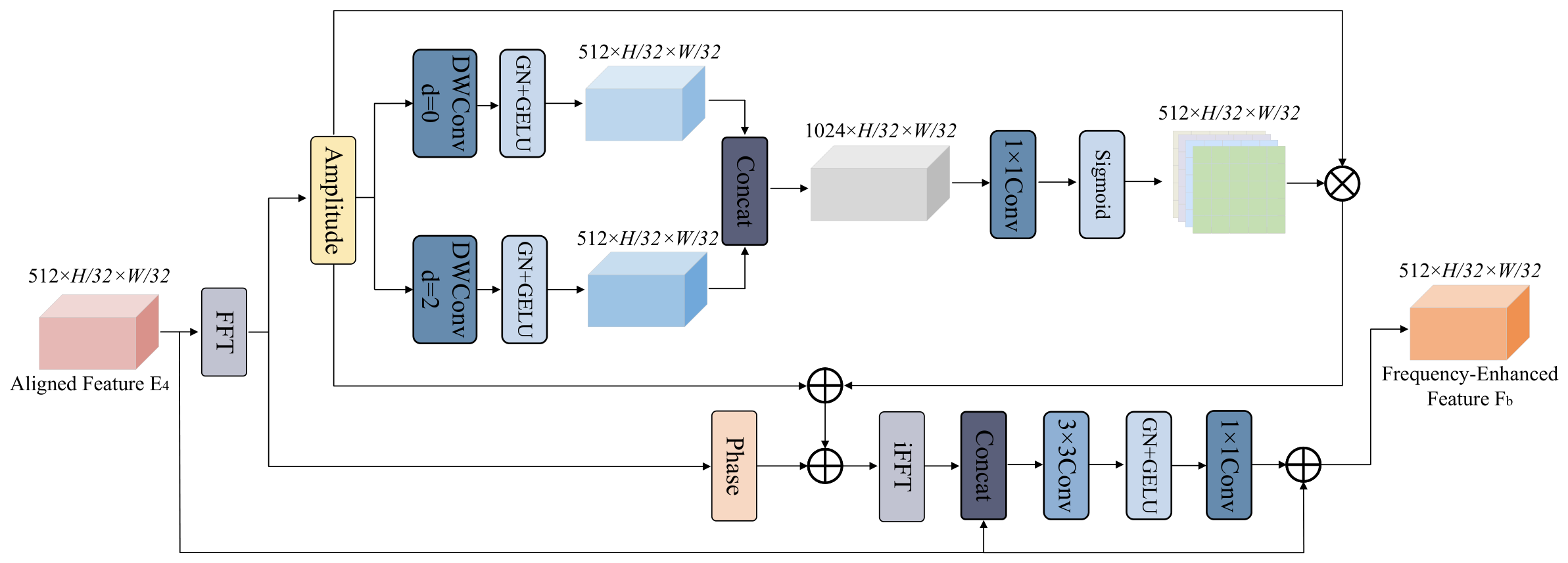
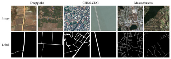
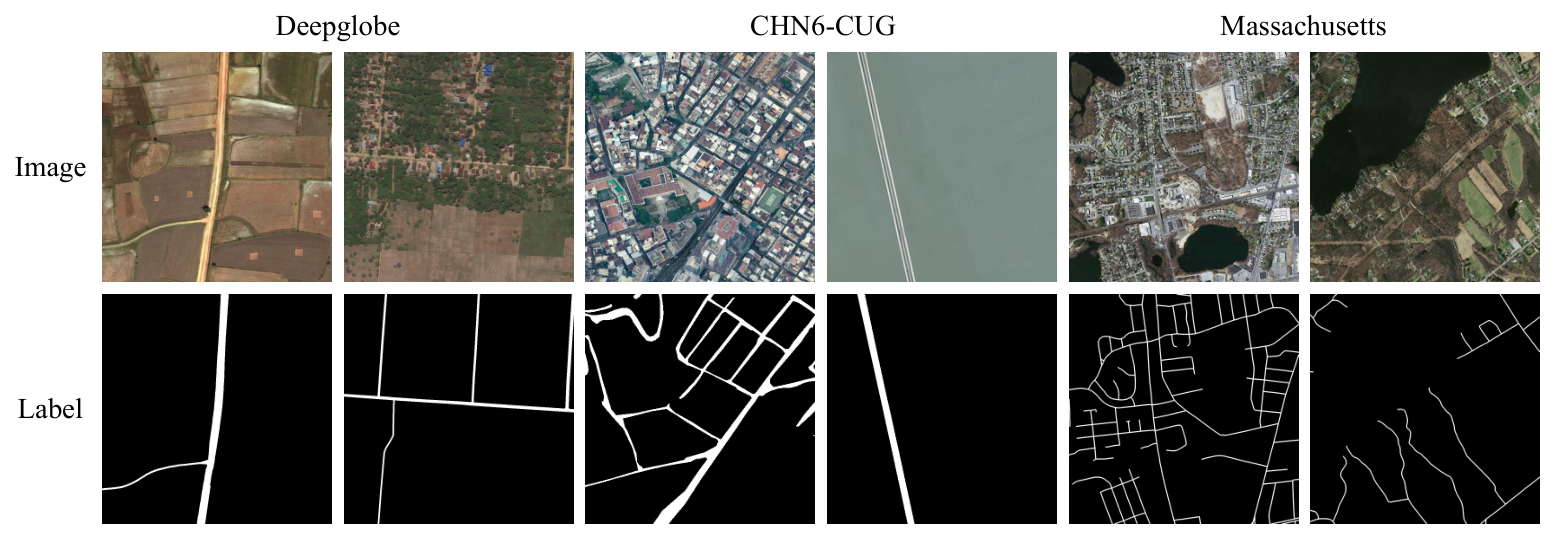
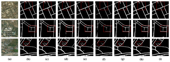
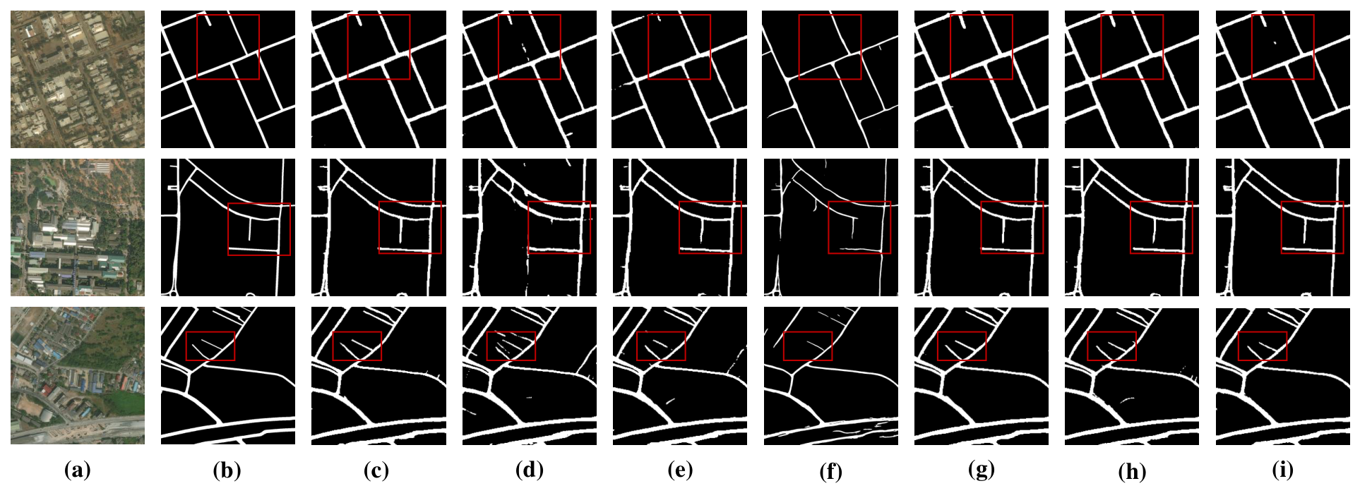
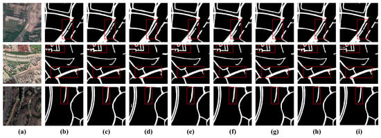
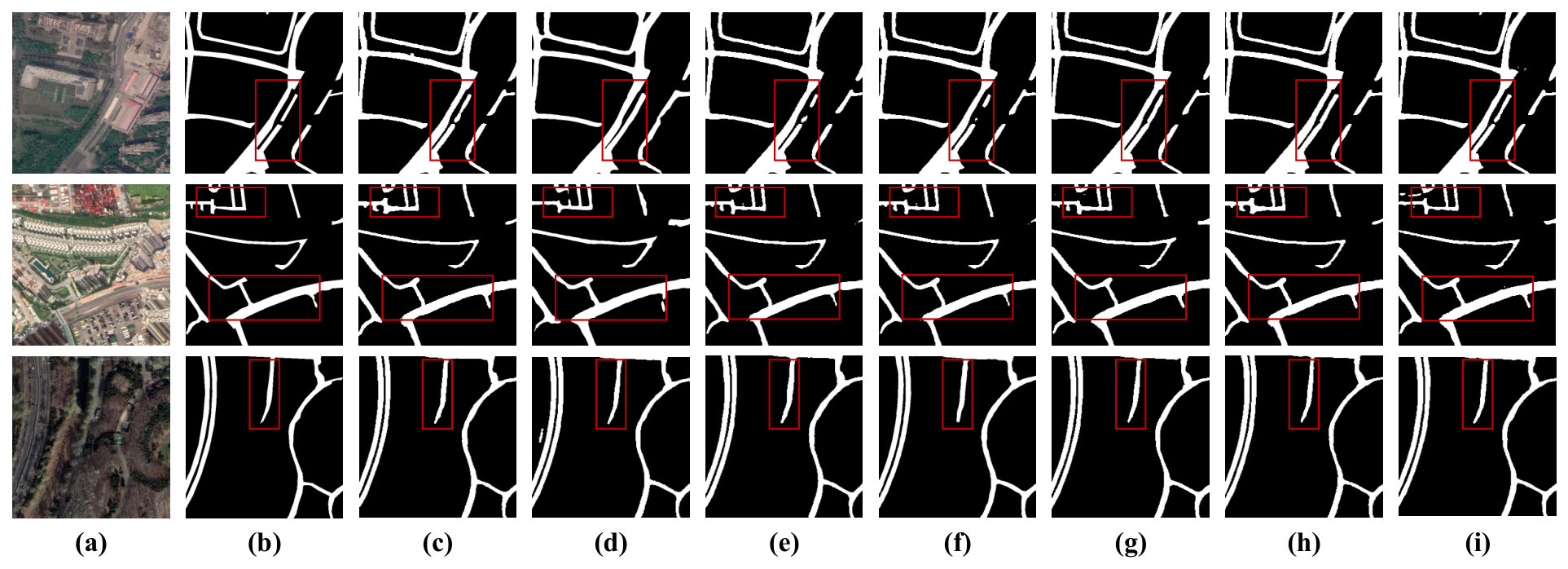
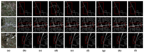
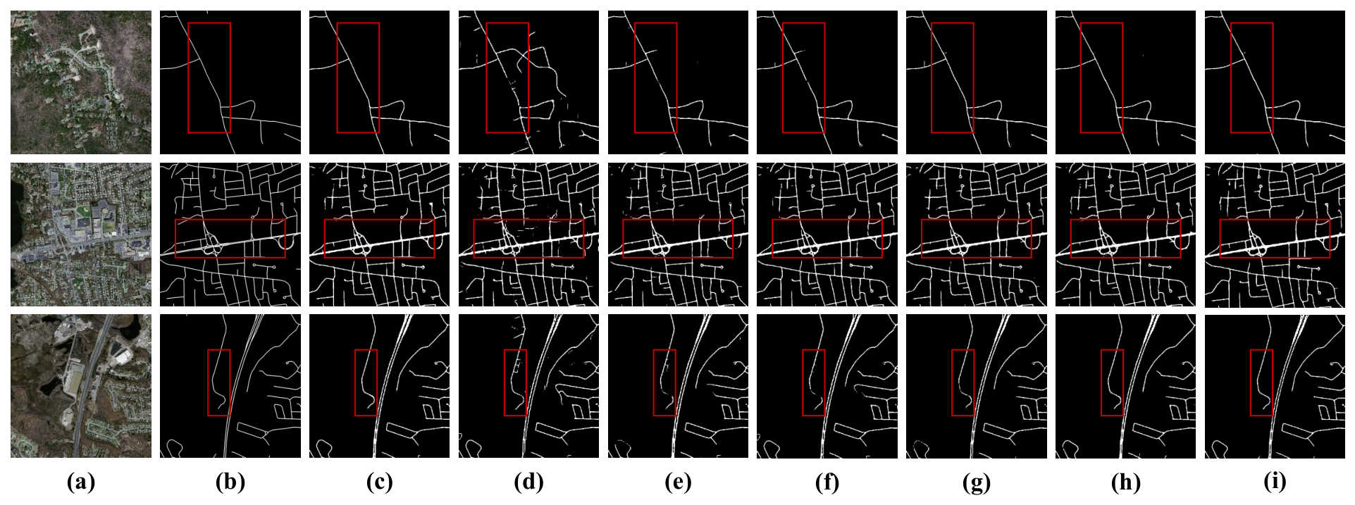
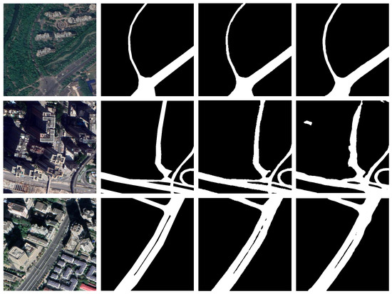
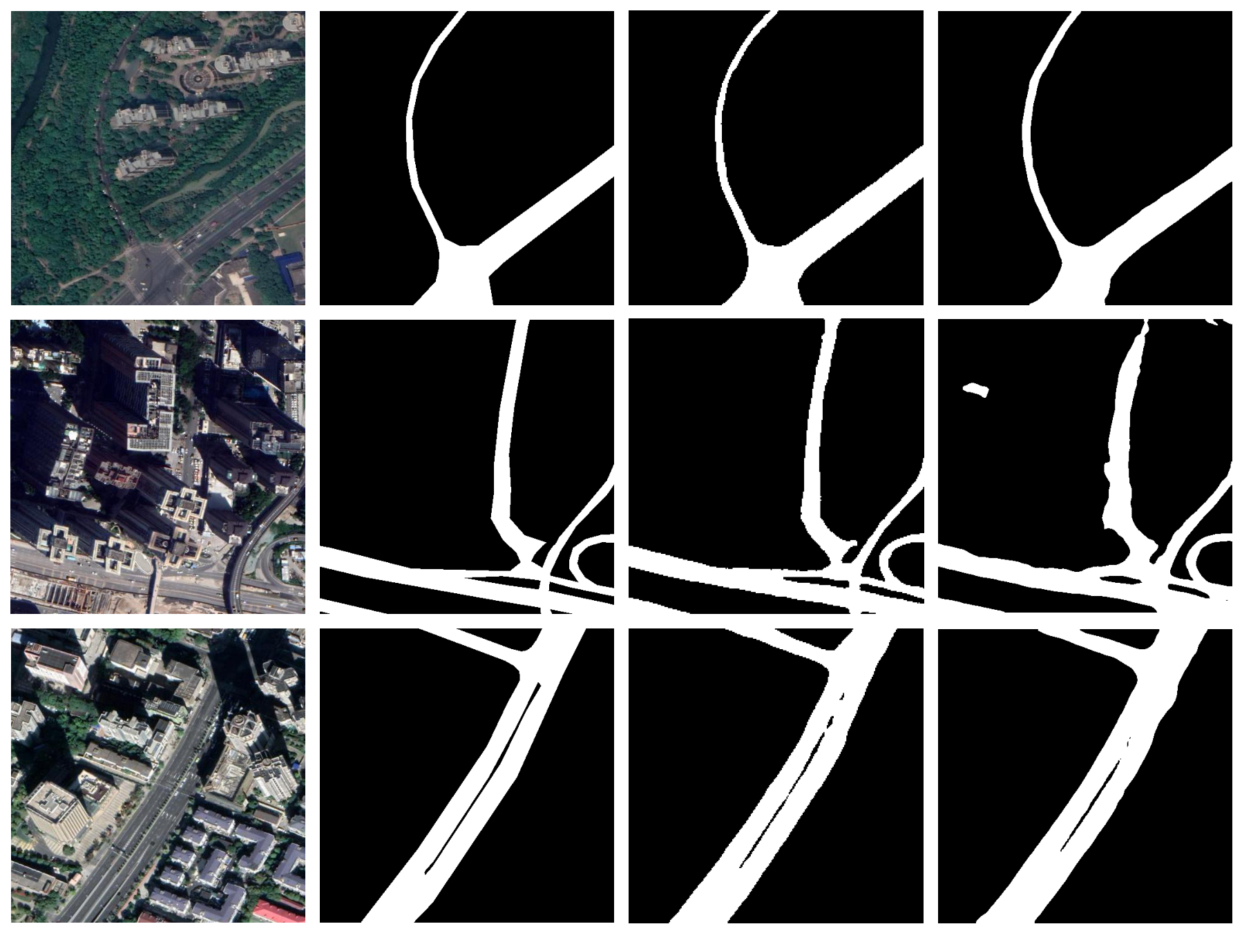

Disclaimer/Publisher’s Note: The statements, opinions and data contained in all publications are solely those of the individual author(s) and contributor(s) and not of MDPI and/or the editor(s). MDPI and/or the editor(s) disclaim responsibility for any injury to people or property resulting from any ideas, methods, instructions or products referred to in the content. |
© 2026 by the authors. Licensee MDPI, Basel, Switzerland. This article is an open access article distributed under the terms and conditions of the Creative Commons Attribution (CC BY) license.