A Mainlobe-Safe Modular Formation Optimization Method for Large-Scale MuSAR with Joint ATI/XTI Baseline Requirements

Highlights

What are the main findings?

• MSMFO achieves balanced ATI/XTI baseline performance under hard mainlobe-safety and minimum-separation constraints, outperforming classical formations and individual optimization strategies.
• The two-level center-layer/module-layer design is validated through controlled formation-scaling studies spanning 8 to 96 satellites, demonstrating its applicability to large-scale MuSAR formation design.

What are the implications of the main findings?

• Mainlobe-safety risks can be mitigated through formation geometry itself, reducing reliance on transmitter shutdown or exclusion-zone-based operational avoidance.
• The modular architecture provides a scalable and physically interpretable design approach for large MuSAR formations requiring simultaneous ATI/XTI performance, synchronization-link availability, and safety.

Abstract

Multistatic synthetic aperture radar (MuSAR) formations with a large number of satellites can provide diverse along-track interferometric (ATI) and cross-track interferometric (XTI) baselines, but increasing formation size introduces strong coupling among baseline performance, intersatellite mainlobe safety, minimum separation, and synchronization-link availability. This paper proposes a Mainlobe-Safe Modular Formation Optimization (MSMFO) method for large-scale MuSAR with joint ATI/XTI baseline requirements. A parameterized relative-motion model and a unified evaluation framework are employed to jointly account for baseline compliance, synchronization-link availability, mainlobe conflicts, and intersatellite separation, with mainlobe conflicts and minimum separation imposed as hard constraints. A Multi-Strategy Cooperative Evolution (MSCE) framework combines complementary global search strategies with local refinement, while a two-level center-layer/module-layer architecture enables scalable formation design. Numerical results show that a six-satellite module achieves XTI and ATI baseline compliance rates of 89.17% each, with 99.98% synchronization-link availability and no safety violations. Compared with the best feasible classical formation, the lower of the two baseline compliance rates is improved by 10.89 percentage points. A controlled study spanning 8–96 satellites maintains consistent module-layer performance, high center-layer compliance, 100% joint availability, and zero global safety violations, providing evidence of modular scalability.

1. Introduction

1.1. Background

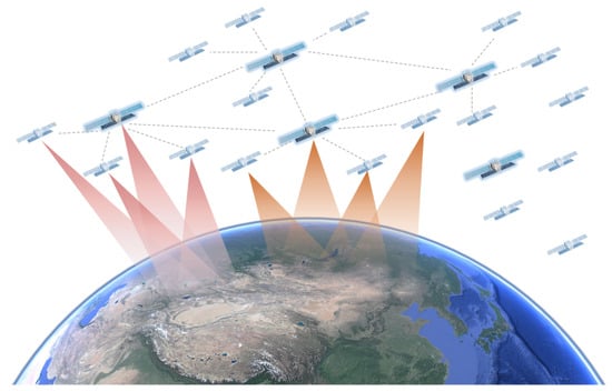
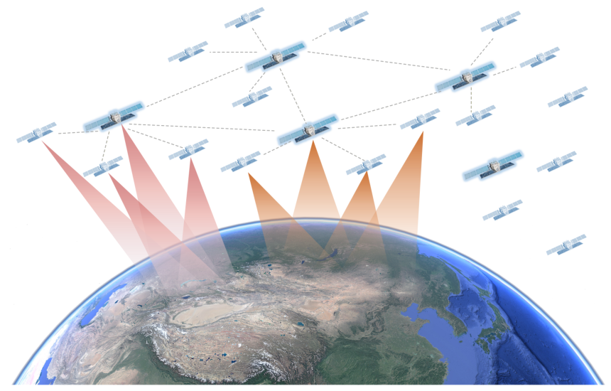
Synthetic aperture radar (SAR) enables day-and-night, all-weather Earth observation and plays an important role in topographic mapping, disaster monitoring, maritime surveillance, and resource exploration [1]. As spaceborne remote-sensing missions increasingly demand higher spatial resolution, shorter revisit times, wider swaths, and multidimensional information acquisition, single-satellite SAR systems face growing limitations in observation-geometry flexibility, interferometric baseline configuration, and mission continuity. By contrast, cooperative multistatic SAR (MuSAR) formations, as illustrated in Figure 1, can generate diverse along-track interferometric (ATI) and cross-track interferometric (XTI) baselines by appropriately designing the intersatellite geometry, thereby supporting moving-target detection, three-dimensional terrain reconstruction, multiangle imaging, and high-precision interferometric measurements [2]. Such formations are therefore receiving increasing attention as a promising architecture for future spaceborne radar systems.

Figure 1. Schematic illustration of a large-scale MuSAR formation for cooperative observation.

In a MuSAR formation, the relative geometry among satellites directly determines the achievable ATI/XTI baseline performance, the geometric availability of intersatellite synchronization links, and system safety. Distributed SAR systems have progressively evolved from single-platform configurations to dual-satellite formations and, more recently, to cooperative MuSAR formations.

The Shuttle Radar Topography Mission (SRTM), conducted in 2000, employed a single-platform dual-antenna configuration to acquire global elevation data and demonstrated the feasibility of spaceborne interferometric mapping [3]. In 2010, Germany’s TanDEM-X mission employed a close-flying two-satellite helix formation to generate a high-precision global digital elevation model, marking an important milestone in the development of distributed SAR [4]. Subsequently, China’s Tianhui-2 (TH-2) dual-satellite system, launched in 2019, employed a helix-like fly-around formation for interferometric mapping [5], while LuTan-1, launched in 2022, adopted a dual-helix formation for bistatic interferometric observations [6]. Hongtu-1, launched in 2023, further extended this concept to a four-satellite cartwheel formation for cooperative MuSAR observations [7]. Looking ahead, Germany’s High-Resolution Wide-Swath (HRWS) mission is being developed with one active radar satellite and three passive companion satellites [8], while ESA’s Harmony mission is planned to deploy two receive-only companion satellites operating in coordination with Sentinel-1 [9]. These developments indicate a continuing evolution of distributed SAR from dual-satellite configurations to cooperative MuSAR systems and from small to large-scale formations.

The need for large-scale MuSAR formations is driven not only by revisit and coverage requirements but also by the demand for denser spatial sampling and greater baseline-orientation diversity within a single pass. For example, Dong et al. [10] investigated MuSAR formation design for single-pass multistatic TomoSAR data acquisition, which requires multiple well-distributed effective baselines in the cross-track or elevation direction to synthesize the elevation aperture. Single-pass acquisition also avoids the temporal decorrelation inherent in repeat-pass observations. Wang et al. [11] investigated ocean-current retrieval using hybrid baselines, an approach that requires joint cross-track and along-track observations. In particular, multiple along-track time lags and baseline configurations can provide additional observational constraints for ocean-current velocity estimation. For systems intended to support TomoSAR, ocean-current retrieval, moving-target detection, and multiangle imaging within the same mission, fixed formations with only two or a few satellites offer limited baseline diversity and may be unable to simultaneously satisfy both XTI and ATI requirements within the same mission window. Increasing the number of satellites allows the formation to be organized into multiple mission-specific subgroups that provide multiple along-track and cross-track baselines simultaneously, thereby increasing spatial-sampling density and observation-geometry diversity. At the same time, the rapidly increasing geometric complexity introduces strong coupling among intersatellite mainlobe conflicts, collision avoidance requirements, synchronization-link availability, and ATI/XTI baseline performance. A formation optimization method is therefore required to jointly account for mission performance, safety constraints, and scalability.

1.2. Problem Statement

The central design objective of a MuSAR formation is to maintain ATI/XTI baselines that satisfy mission requirements throughout orbital operation while avoiding collisions, maintaining high synchronization-link availability and preventing hazardous intersatellite illumination by the SAR mainlobe. Intersatellite mainlobe illumination constitutes a distinctive safety constraint in SAR formation design that is generally absent from conventional satellite formations. Because SAR payloads typically employ high-power transmission, a satellite entering the mainlobe of another satellite’s SAR antenna may be exposed to strong electromagnetic energy that can couple into its sensitive electronics or receiver channels, potentially causing component damage or system anomalies [12,13]. Consequently, intersatellite mainlobe illumination should not be treated merely as a conventional link-blockage issue but should instead be imposed as a hard safety constraint in formation design.

For receive-only satellites, the SAR antenna mainlobe defines the primary receiving region. If another satellite enters the receive mainlobe, it may introduce undesired scattering, blockage, or additional propagation paths, thereby contaminating the received echoes [14]. Accordingly, the term intersatellite mainlobe conflict is used in this paper to encompass both transmit-mainlobe illumination and receive-mainlobe intrusion, both of which are treated as unacceptable geometric conditions in formation design.

Existing missions typically mitigate transmit-mainlobe illumination risk through mission planning and operational scheduling. TanDEM-X, for example, establishes specific exclusion zones along the orbit during close formation flying to prevent one satellite from being illuminated by the other satellite’s SAR mainlobe, thereby reducing the risk of damage to onboard electronic components [12,13]. Independent ground and onboard checks are used to inhibit radar transmission whenever one spacecraft may cross the radar beam of the other. Although this strategy can reduce the risk of intersatellite mainlobe illumination, it also limits radar data acquisition over the ground regions corresponding to those orbital segments, resulting in local observation gaps. For dual-satellite systems or small formations, such planning-based avoidance remains operationally manageable. As the number of satellites increases, however, the number of satellite pairs subject to potential mainlobe illumination grows rapidly, making such risks increasingly difficult to manage. The number of satellite pairs requiring monitoring for potential mainlobe illumination increases substantially, while exclusion zones may become more frequent and complex, further reducing effective observation time and the spatial coverage of acquired data. In other words, the conventional strategy of disabling transmission in risk regions is simple and reliable, but it creates local observation gaps and imposes an increasing operational burden as the formation size grows, making it less suitable for continuous, high-coverage operation of large-scale MuSAR formations.

Classical configurations [15] such as the cartwheel, pendulum, and helix exhibit well-defined relative-motion patterns and are readily interpretable from an engineering perspective, making them well suited to the design of small formations [16,17]. Their geometric degrees of freedom are limited, however, and they tend to favor a specific type of baseline geometry. Consequently, it is difficult to simultaneously maintain high XTI and ATI baseline compliance rates within the same mission, and these configurations offer limited adaptability to changes in the required baseline ranges, satellite count, and safety constraints [16]. These limitations become more pronounced as the number of satellites increases, particularly when the formation must simultaneously satisfy requirements for mainlobe safety, intersatellite separation, synchronization-link availability, and joint ATI/XTI baseline performance. Conversely, optimizing all satellites simultaneously within a single global problem causes the number of design variables and constraint interactions to grow rapidly, reducing optimization efficiency, making feasible solutions more difficult to identify, and complicating the formation architecture. The key challenge is therefore to mitigate intersatellite mainlobe conflicts through formation design, without relying on transmitter shutdown to avoid transmit-mainlobe illumination over specific orbital segments, while maintaining high and balanced ATI/XTI baseline performance and enabling modular scalability to large-scale MuSAR formations.

1.3. Comparison with Closely Related Formation-Design Methods

Recent SAR-specific formation studies provide closer points of comparison than classical geometries alone. Zhang et al. [16] proposed the superpolyhedron formation by combining dual-helix and pendulum structures and optimizing effective cross-track and along-track interferometric-baseline coverage within a prescribed topology; their formulation also includes an intersatellite safe-distance constraint. Dong et al. [10] developed a single-pass multistatic TomoSAR formation-design method based on equivalent phase centers, in which the transceiver configuration and effective perpendicular baselines are designed to meet tomographic-resolution, ambiguity, and sampling requirements. These methods establish important recent benchmarks, but their task scopes differ from the multi-constraint, large-scale MuSAR problem considered here.

This comparison clarifies that simultaneous XTI/ATI consideration alone is not claimed as the novelty of MSMFO, because the superpolyhedron method already optimizes effective XTI/ATI coverage within a prescribed topology. The specific contribution of MSMFO is the unified treatment of XTI/ATI task metrics, synchronization-link availability, intersatellite mainlobe conflicts, and minimum separation through one physical formation-design interface, with the two safety requirements enforced as hard constraints. Unlike the topology-specific superpolyhedron formulation and the transceiver-configuration design used for single-pass TomoSAR, MSMFO searches a bounded and physically interpretable relative-motion parameter space without requiring a predefined classical or superpolyhedron geometry. In addition, its center-layer/module-layer architecture separates long-baseline intermodule design from reusable local-module design and performs global safety verification after the two levels are combined.

1.4. Contributions

The main contributions of this paper are summarized as follows. A Mainlobe-Safe Modular Formation Optimization (MSMFO) method is developed for MuSAR formation design under joint ATI/XTI baseline requirements. The method incorporates ATI/XTI baseline compliance, synchronization-link availability, intersatellite mainlobe conflicts, and intersatellite separation into a unified evaluation framework, in which mainlobe conflicts and minimum separation are treated as hard constraints. To address the resulting nonlinear and highly constrained optimization problem, a Multi-Strategy Cooperative Evolution (MSCE) framework is introduced by combining complementary global search strategies with local refinement, thereby improving the robustness of the search for high-quality feasible formations.

To support large-scale MuSAR formation design, a two-level center-layer/module-layer strategy is further introduced, in which the long-baseline intermodule geometry is optimized at the center layer and the local intramodule geometry is designed at the module layer, followed by global safety verification. The proposed framework is evaluated through single-module optimization, comparisons with individual optimization strategies and classical formations, and a controlled multi-scale modular study spanning 8–96 satellites. The results demonstrate that MSMFO can achieve balanced ATI/XTI baseline performance while satisfying the prescribed safety constraints and provide evidence of modular scalability.

1.5. Organization of This Paper

The remainder of this paper is organized as follows. Section 2 establishes the theoretical foundations and evaluation metrics for MuSAR formation optimization. Section 3 presents the MSMFO method. Section 4 evaluates the mission performance, safety, and scalability of MSMFO through single-module optimization, comparisons among optimization strategies, comparisons with classical formations, and a controlled modular scaling study spanning 8–96 satellites. Section 5 discusses the limitations of the current geometric model and the higher-fidelity payload models and engineering constraints to be incorporated in future work. Section 6 concludes the paper. For reproducibility, Appendix A provides the orbital parameters corresponding to the main results presented in this paper.

2. Fundamentals and Metrics for MuSAR Formation Optimization

This section establishes the theoretical foundations and evaluation metrics for mainlobe-safe formation optimization. The coordinate system and notation for a MuSAR formation are first introduced, and a parameterized relative-motion model is used to describe periodic intersatellite motion. The ATI/XTI baseline compliance rates, intersatellite synchronization-link availability, intersatellite SAR mainlobe conflicts, and the minimum intersatellite separation metric are then defined. Finally, these metrics are integrated into a unified evaluation interface for subsequent formation generation, constraint handling, and composite evaluation in MSMFO.

2.1. Formation Scenario and Coordinate System

Consider a cooperative MuSAR formation consisting of N SAR satellites. Satellite 1 is selected as the reference satellite, and the global satellite indices use one-based global numbering. The remaining satellites are described relative to the reference satellite. For an arbitrary satellite i, let its position vector in an inertial or Earth-centered orbital reference frame be denoted by $r_i\left(t\right)$. For any two satellites i and j, their relative position vector is defined as

$${\mathit{\rho }}_{ij}\left(t\right)={\mathbf{r}}_j\left(t\right)-{\mathbf{r}}_i\left(t\right).$$

(1)

The reference-satellite orbital frame, i.e., the Local Vertical Local Horizontal (LVLH) frame, is used to describe intersatellite relative motion [16]. Its origin is located at the center of mass of the reference satellite. The x-axis is radial and points away from the Earth’s center; the y-axis is tangential to the orbit and approximately represents the along-track direction; and the z-axis is normal to the orbital plane and approximately represents the cross-track direction. In this frame, the position of the i-th satellite relative to the reference satellite is expressed as

$${\mathit{\rho }}_i\left(t\right)=\left[\begin{array}{c}{x}_i\left(t\right)\hfill \\ y_i\left(t\right)\hfill \\ z_i\left(t\right)\hfill \end{array}\right],i=1,2,\dots ,N-1$$

(2)

where i denotes the satellite index relative to the reference satellite and t denotes orbital time. To evaluate formation performance over one orbital period, the period T is discretized into K sampling instants:

$$t_k={\displaystyle \frac{k-1}{K}}T,k=1,2,\dots ,K.$$

(3)

At each sampling instant, the intersatellite relative positions, ATI/XTI baselines, synchronization-link geometry, mainlobe pointing geometry, and intersatellite distances are evaluated. Statistics over all sampling instants are then used to compute the evaluation metrics for the complete orbital period.

2.2. Parameterized Relative-Motion Model

To improve the physical interpretability and optimization efficiency of formation design, a parameterized relative-motion model is adopted to describe periodic intersatellite motion. The model is based on the classical Clohessy-Wiltshire (C-W) relative-motion equations [18]. Under the assumption of a near-circular reference orbit, the motion of a satellite relative to the reference satellite in the LVLH frame is governed by

$$\left\{\begin{array}{c}\ddot{x}-2n\dot{y}-3n^{2}x=0,\hfill \\ \ddot{y}+2n\dot{x}=0,\hfill \\ \ddot{z}+n^{2}z=0,\hfill \end{array}\right.$$

(4)

where n is the mean angular rate of the reference orbit. The motion of the i-th satellite relative to the reference satellite is parameterized as

$$\left\{\begin{array}{cc}\hfill x_i\left(t\right)& =-p_{i}cos\left(nt+{\theta }_i\right),\hfill \\ \hfill y_i\left(t\right)& =2p_{i}sin\left(nt+{\theta }_i\right)+l_i,\hfill \\ \hfill z_i\left(t\right)& =s_{i}sin\left(nt+{\theta }_i-{\alpha }_i\right).\hfill \end{array}\right.$$

(5)

where $p_i$ denotes the amplitude of the radial/along-track elliptical motion, $s_i$ denotes the normal or cross-track amplitude, ${\theta }_i$ is the in-plane phase, ${\alpha }_i$ is the cross-track phase offset, and $l_i$ is the mean along-track position offset. Accordingly, the relative-motion parameters of the i-th satellite are written as

$${\mathbf{q}}_i={\left[\begin{array}{ccccc}{p}_i\hfill & s_i\hfill & {\alpha }_i\hfill & {\theta }_i\hfill & l_i\hfill \end{array}\right]}^{\mathrm{T}}.$$

(6)

For a formation of N satellites, after one satellite is selected as the reference, the relative-motion parameters of the remaining $N-1$ satellites can be represented as

$$\mathbf{Q}={\left[\begin{array}{cccc}{\mathbf{q}}_1^{\mathrm{T}}\hfill & {\mathbf{q}}_2^{\mathrm{T}}\hfill & \dots \hfill & {\mathbf{q}}_{N-1}^{\mathrm{T}}\hfill \end{array}\right]}^{\mathrm{T}}.$$

(7)

This parameterization represents periodic intersatellite relative motion using a finite-dimensional set of continuous variables. The subsequent optimization searches this parameter space for formations that satisfy both mission-performance and safety requirements.

It should be noted that the C-W-based relative-motion model is used here as a parameterized representation of the formation design variables rather than as the final orbit-propagation model. For candidate evaluation, the relative-motion parameters are mapped to the corresponding orbital elements, which are subsequently propagated using the J2-perturbed orbital model [19]. Thus, the C-W parameterization provides a compact and physically interpretable design space, whereas the J2 model is used to evaluate the orbital evolution of each candidate formation.

2.3. ATI/XTI Baseline Compliance Metrics

The mission capability of a MuSAR formation is largely determined by its intersatellite baselines. According to baseline orientation, this work focuses on ATI and XTI baselines. ATI baselines primarily affect moving-target detection, velocity estimation, and along-track interferometry, whereas XTI baselines primarily affect height retrieval, three-dimensional imaging, and cross-track interferometric measurements [2,16].

In the LVLH frame, the relative position of arbitrary satellites i and j at time $t_k$ is written as

$${\mathit{\rho }}_{ij}\left(t_k\right)=\left[\begin{array}{c}\Delta x_{ij}\left(t_k\right)\hfill \\ \Delta y_{ij}\left(t_k\right)\hfill \\ \Delta z_{ij}\left(t_k\right)\hfill \end{array}\right].$$

(8)

For a specified target and transmit–receive geometry, let ${\widehat{\mathit{e}}}_{\mathrm{LOS}}\left(t_k\right)$ denote the unit vector along the radar line of sight and let ${\widehat{\mathit{e}}}_{\mathrm{AT}}\left(t_k\right)$ denote the along-track unit vector. Under the zero-squint observation geometry considered in this paper, the unit vector perpendicular to the LOS within the range plane is defined as

$${\widehat{\mathit{e}}}_{\perp }\left(t_k\right)={\displaystyle \frac{{\widehat{\mathit{e}}}_{\mathrm{AT}}\left(t_k\right)\times {\widehat{\mathit{e}}}_{\mathrm{LOS}}\left(t_k\right)}{∥{\widehat{\mathit{e}}}_{\mathrm{AT}}\left(t_k\right)\times {\widehat{\mathit{e}}}_{\mathrm{LOS}}\left(t_k\right)∥}}.$$

The perpendicular interferometric baseline is generally denoted by $B_{\perp }$; following [16], it is also denoted by $B^{\mathrm{XTI}}$ in this paper. Accordingly, the ATI and effective perpendicular XTI baselines used in the optimization are defined as

$$B_{ij}^{\mathrm{ATI}}\left(t_k\right)=\left|{\mathit{\rho }}_{ij}^{\mathrm{T}}\left(t_k\right){\widehat{\mathit{e}}}_{\mathrm{AT}}\left(t_k\right)\right|=\left|\Delta y_{ij}\left(t_k\right)\right|,$$

(9)

$$B_{ij}^{\mathrm{XTI}}\left(t_k\right)\equiv B_{\perp ,ij}\left(t_k\right)=\left|{\mathit{\rho }}_{ij}^{\mathrm{T}}\left(t_k\right){\widehat{\mathbf{e}}}_{\perp }\left(t_k\right)\right|.$$

(10)

The effective ATI time lag corresponding to a satellite pair is

$${\tau }_{ij}^{\mathrm{ATI}}\left(t_k\right)={\displaystyle \frac{B_{ij}^{\mathrm{ATI}}\left(t_k\right)}{v_{\mathrm{sat}}}},$$

where $v_{\mathrm{sat}}$ is the satellite speed. The physical relationships between the baseline metrics and the corresponding interferometric performance can be expressed as [16]

$$h_{\mathrm{amb}}={\displaystyle \frac{\lambda Rsin\theta }{2B^{\mathrm{XTI}}}},$$

and

$$V_{\mathrm{md}}={\displaystyle \frac{\lambda v_{\mathrm{sat}}\eta }{2\pi B^{\mathrm{ATI}}}},$$

where $h_{\mathrm{amb}}$ denotes the height of ambiguity, $V_{\mathrm{md}}$ denotes the minimum detectable velocity, and $\lambda$, R, $\theta$, and $\eta$ denote the radar wavelength, slant range, incidence angle, and phase-detection threshold, respectively. These relationships connect the XTI and ATI baseline-compliance metrics to the height of ambiguity and the minimum detectable velocity for the specified observation geometry.

Let the mission-required ATI baseline range be given by

$$B_{min}^{\mathrm{ATI}}\le B_{ij}^{\mathrm{ATI}}\left(t_k\right)\le B_{max}^{\mathrm{ATI}},$$

(11)

and the corresponding XTI baseline range by

$$B_{min}^{\mathrm{XTI}}\le B_{ij}^{\mathrm{XTI}}\left(t_k\right)\le B_{max}^{\mathrm{XTI}}.$$

(12)

If the baseline of a given satellite pair falls within the corresponding range at a given time instant, that satellite pair is considered to satisfy the associated baseline requirement at that instant. The indicator functions are defined as

$$I_{ij}^{\mathrm{ATI}}\left(t_k\right)=\left\{\begin{array}{cc}1,\hfill & B_{min}^{\mathrm{ATI}}\le B_{ij}^{\mathrm{ATI}}\left(t_k\right)\le B_{max}^{\mathrm{ATI}},\hfill \\ 0,\hfill & \mathrm{otherwise},\hfill \end{array}\right.$$

(13)

$$I_{ij}^{\mathrm{XTI}}\left(t_k\right)=\left\{\begin{array}{cc}1,\hfill & B_{min}^{\mathrm{XTI}}\le B_{ij}^{\mathrm{XTI}}\left(t_k\right)\le B_{max}^{\mathrm{XTI}},\hfill \\ 0,\hfill & \mathrm{otherwise}.\hfill \end{array}\right.$$

(14)

Let ${\mathcal{P}}_b$ denote the set of satellite pairs included in baseline evaluation. The ATI and XTI baseline compliance rates over one orbital period are, respectively, defined as

$$C_{\mathrm{ATI}}={\displaystyle \frac{1}{\left|{\mathcal{P}}_b\right|K}}{\displaystyle \sum _{\left(i,j\right)\in {\mathcal{P}}_b}}{\displaystyle \sum _{k=1}^K}{I}_{ij}^{\mathrm{ATI}}\left(t_k\right),$$

(15)

$$C_{\mathrm{XTI}}={\displaystyle \frac{1}{\left|{\mathcal{P}}_b\right|K}}{\displaystyle \sum _{\left(i,j\right)\in {\mathcal{P}}_b}}{\displaystyle \sum _{k=1}^K}{I}_{ij}^{\mathrm{XTI}}\left(t_k\right).$$

(16)

The two marginal compliance rates do not by themselves indicate whether the same satellite pair satisfies both baseline requirements at the same sampling instant. To quantify this simultaneous overlap, the pairwise joint-compliance indicator is defined as

$$I_{ij}^{\mathrm{joint}}\left(t_k\right)=I_{ij}^{\mathrm{ATI}}\left(t_k\right)I_{ij}^{\mathrm{XTI}}\left(t_k\right).$$

The simultaneous joint compliance rate over all evaluated pair-time samples is then

$$C_{\mathrm{joint}}={\displaystyle \frac{1}{\left|{\mathcal{P}}_b\right|K}}{\displaystyle \sum _{\left(i,j\right)\in {\mathcal{P}}_b}}{\displaystyle \sum _{k=1}^K}{I}_{ij}^{\mathrm{joint}}\left(t_k\right),$$

and the joint availability, which measures the fraction of sampled instants at which at least one evaluated pair simultaneously satisfies both requirements, is

$$A_{\mathrm{joint}}={\displaystyle \frac{1}{K}}{\displaystyle \sum _{k=1}^K}\mathbf{1}\left[\sum _{\left(i,j\right)\in {\mathcal{P}}_b}{I}_{ij}^{\mathrm{joint}}\left(t_k\right)\ge 1\right],$$

where $\mathbf{1}[·]$ is the indicator function. In this paper, “joint ATI/XTI requirements” means that the ATI and XTI requirements are considered concurrently in the same formation-design problem. When same-pair, same-time satisfaction is intended, it is reported explicitly using $C_{\mathrm{joint}}$ and $A_{\mathrm{joint}}$. The term $min\left(C_{\mathrm{XTI}},C_{\mathrm{ATI}}\right)$ used later in the composite score is a balance-oriented term and is not a substitute for the simultaneous-overlap metrics.

Both $C_{\mathrm{ATI}}$ and $C_{\mathrm{XTI}}$ lie in $[0,1]$. The closer these values are to 1, the higher the proportion of the orbital period over which the formation satisfies the corresponding baseline requirement.

2.4. Intersatellite Synchronization-Link Availability Metric

MuSAR systems require intersatellite time and phase synchronization, and any satellite may participate in the transmission or reception of synchronization signals [20,21,22]. Therefore, the geometric clearance of intersatellite synchronization links is an important consideration in formation design. A third satellite located close to the direct propagation path between two communicating satellites may obstruct the line of sight or introduce additional scattering paths, thereby increasing the risk of multipath-induced amplitude, phase, or time errors and degrading cooperative MuSAR imaging performance [14].

Consider a synchronization link between satellites i and j, represented by the line segment $\overline{ij}$. For an arbitrary third satellite h, define the minimum distance from satellite h to link $\overline{ij}$ as

$$d_{h,ij}\left(t_k\right)=dist\left({\mathbf{r}}_h\left(t_k\right),\overline{{\mathbf{r}}_i\left(t_k\right){\mathbf{r}}_j\left(t_k\right)}\right),$$

(17)

where $\mathrm{dist}(·)$ denotes the shortest distance from a point to a line segment. Let $d_{\mathrm{link}}$ be the geometric-clearance threshold for a synchronization link. If the minimum distance from every third satellite to the link segment is no smaller than this threshold, link $(i,j)$ is considered geometrically clear at that instant. The corresponding link-availability indicator is defined as

$$I_{ij}^{\mathrm{link}}\left(t_k\right)=\left\{\begin{array}{cc}1,\hfill & \underset{h\ne i,j}{min}{d}_{h,ij}\left(t_k\right)\ge d_{\mathrm{link}},\hfill \\ 0,\hfill & \mathrm{otherwise}.\hfill \end{array}\right.$$

(18)

Let ${\mathcal{P}}_l$ denote the set of synchronization links to be evaluated. The synchronization-link availability over one orbital period is defined as

$$C_{\mathrm{link}}={\displaystyle \frac{1}{\left|{\mathcal{P}}_l\right|K}}{\displaystyle \sum _{\left(i,j\right)\in {\mathcal{P}}_l}}{\displaystyle \sum _{k=1}^K}{I}_{ij}^{\mathrm{link}}\left(t_k\right).$$

(19)

This metric characterizes the ability of the formation to maintain geometrically clear synchronization links throughout the orbital period. A value of $C_{\mathrm{link}}$ closer to 1 indicates a lower risk of obstruction or close-proximity interference by third-party satellites along the link path.

2.5. Intersatellite SAR Mainlobe Conflict Metric

Intersatellite SAR mainlobe conflict is a key safety and operational issue in MuSAR formation design. Because a SAR antenna mainlobe is used for both transmission and reception, the consequence of another satellite entering the mainlobe depends on the operating mode of the corresponding SAR payload. For a transmitting satellite, another satellite entering its transmit mainlobe may be exposed to high-power electromagnetic radiation, potentially causing excessive power coupling into receiver channels or sensitive electronic components. For a receive-only satellite, another radiating satellite inside the antenna’s high-gain receiving region may introduce direct-path interference and image artifacts [14]. Therefore, both transmit-mainlobe illumination and receive-mainlobe intrusion are regarded as unacceptable mainlobe conflicts in this paper and are treated as hard constraints in formation design.

Let the unit vector of the SAR antenna mainlobe of satellite i at time $t_k$ be

$${\mathbf{b}}_i\left(t_k\right).$$

(20)

This vector is determined by the satellite attitude, side-looking direction, and radar-beam pointing. The unit vector from satellite i to satellite j is

$${\mathbf{e}}_{ij}\left(t_k\right)={\displaystyle \frac{{\mathbf{r}}_j\left(t_k\right)-{\mathbf{r}}_i\left(t_k\right)}{∥{\mathbf{r}}_j\left(t_k\right)-{\mathbf{r}}_i\left(t_k\right)∥}}.$$

(21)

The angular separation of satellite j from the mainlobe axis of satellite i is then

$${\varphi }_{ij}\left(t_k\right)=arccos\left({\mathbf{b}}_i^{\mathrm{T}}\left(t_k\right){\mathbf{e}}_{ij}\left(t_k\right)\right).$$

(22)

Let the SAR antenna mainlobe half-angle be ${\theta }_{\mathrm{ML}}$ and the mainlobe safety margin be ${\theta }_{\mathrm{margin}}$. The angular safety threshold is defined as

$${\theta }_{\mathrm{safe}}={\theta }_{\mathrm{ML}}+{\theta }_{\mathrm{margin}}.$$

(23)

Here, ${\theta }_{\mathrm{margin}}$ is an additional angular margin that accounts for attitude and antenna-alignment errors, relative-navigation uncertainty, beam-model simplification, and intersample angular motion.

The mainlobe-conflict indicator is defined as

$$I_{ij}^{\mathrm{ML}}\left(t_k\right)=\left\{\begin{array}{cc}1,\hfill & {\varphi }_{ij}\left(t_k\right)\le {\theta }_{\mathrm{safe}},\hfill \\ 0,\hfill & \mathrm{otherwise}.\hfill \end{array}\right.$$

(24)

Under this definition, $I_{ij}^{\mathrm{ML}}\left(t_k\right)=1$ indicates that satellite j enters the prescribed SAR mainlobe region of satellite i at time $t_k$. A mainlobe conflict is therefore declared whenever one satellite enters the prescribed mainlobe region of another satellite. The indicator $I_{ij}^{\mathrm{ML}}$ is directional, and all directed satellite pairs are checked at every sampled instant. The total number of mainlobe conflicts over one orbital period is defined as

$$N_{\mathrm{ML}}={\displaystyle \sum _{k=1}^K}{\displaystyle \sum _{i=1}^N}{\displaystyle \sum _{\begin{array}{c}j=1\\ j\ne i\end{array}}^N}{I}_{ij}^{\mathrm{ML}}\left(t_k\right).$$

(25)

Here, $N_{\mathrm{ML}}$ is a dimensionless discrete occurrence count. One count corresponds to one directed satellite-pair–sample occurrence for which $I_{ij}^{\mathrm{ML}}\left(t_k\right)=1$. Thus, the ordered pairs $(i,j)$ and $(j,i)$ are counted separately, and consecutive violating samples for the same ordered pair are also counted separately. Accordingly, $N_{\mathrm{ML}}$ should not be interpreted as the number of independent continuous-time conflict events.

2.6. Minimum Intersatellite Separation Metric

In addition to intersatellite mainlobe conflicts, intersatellite separation is a fundamental safety metric for MuSAR formation evaluation. The distance between two arbitrary satellites is defined as

$$d_{ij}\left(t_k\right)=∥{\mathbf{r}}_j\left(t_k\right)-{\mathbf{r}}_i\left(t_k\right)∥.$$

(26)

The minimum intersatellite separation over the entire orbital period is defined as

$$d_{min}=\underset{k}{min}\underset{i<j}{min}{d}_{ij}\left(t_k\right).$$

(27)

Let $d_{\mathrm{safe}}$ denote the prescribed minimum intersatellite separation threshold. The separation requirement is satisfied when $d_{\min }\ge d_{\mathrm{safe}}$. For numerical reporting, occurrences of intersatellite separation below $d_{\mathrm{safe}}$ are additionally counted as minimum-separation violations.

2.7. Evaluation Metrics and Optimization Interface

In summary, the five evaluation quantities used in this paper are consistent with the preceding definitions: the XTI and ATI baseline compliance rates are denoted by $C_{\mathrm{XTI}}$ and $C_{\mathrm{ATI}}$, respectively; synchronization-link availability is denoted by $C_{\mathrm{link}}$; the total number of mainlobe conflicts is denoted by $N_{\mathrm{ML}}$; and the minimum intersatellite separation over the orbital period is denoted by $d_{\min }$. The first three quantify mission performance and synchronization-link availability, whereas the latter two are used to construct safety constraints.

For an arbitrary set of relative-motion parameters Q, orbital-period sampling and geometric calculations yield the following metric mapping:

$$\mathbf{Q}\to \left(C_{\mathrm{XTI}},C_{\mathrm{ATI}},C_{\mathrm{link}},N_{\mathrm{ML}},d_{min}\right).$$

(28)

This mapping forms the evaluation basis for the optimization method developed in the following section.

3. Mainlobe-Safe Modular Formation Optimization

Section 2 established the evaluation metrics for mainlobe-safe MuSAR formations, including the parameterized relative-motion model, ATI/XTI baseline compliance rates, synchronization-link availability, the number of mainlobe conflicts, and the minimum intersatellite separation. Building on these definitions, this section presents the MSMFO method. MSMFO uses the parameterized relative-motion model as its formation representation, converts the above metrics into optimization objectives, hard safety constraints, and a composite score, and employs the MSCE framework to search for feasible solutions in a complex formation design space with multiple coupled constraints. To address the high dimensionality, strong constraint coupling, and organizational complexity associated with direct optimization of large-scale MuSAR formations, a two-level center-layer/module-layer design is further introduced to decompose the overall problem into interpretable and scalable subproblems.

3.1. Overall Methodology

The principal difficulty in MuSAR formation optimization is the strong coupling between mission objectives and safety constraints. On the one hand, adequate cross-track and along-track relative separations are required to generate effective XTI/ATI baselines. On the other hand, intersatellite separation and spatial distribution also affect intersatellite SAR mainlobe conflicts, collision risk, and synchronization-link geometry. Therefore, optimizing only the ATI/XTI baseline metrics may yield solutions that violate safety constraints, whereas simply increasing intersatellite separation to avoid risk may reduce cooperative observation capability or result in an excessively large formation extent.

The basic idea of MSMFO is to search the parameterized relative-motion space for formations that provide high mission performance while satisfying the safety constraints, such that intersatellite mainlobe conflicts are mitigated through the formation geometry itself, without relying on transmitter shutdown to avoid transmit-mainlobe illumination over selected orbital segments. The overall procedure comprises three main stages. First, the formation design hierarchy is determined according to the mission requirements and satellite count. Second, each candidate formation is sampled over one orbital period and evaluated using the evaluation metrics established in Section 2. Third, the MSCE framework iteratively searches the constrained space for feasible formations with favorable composite performance.

Unlike conventional fixed-geometry design, MSMFO does not require the formation to strictly follow a predefined classical shape. Instead, it searches within a physically interpretable relative-motion parameter space for geometries that satisfy the mission requirements. Compared with direct global optimization of all satellite parameters, the modular design reduces the number of variables and the complexity of constraint checking while providing a more structured architecture and improved scalability for large-scale MuSAR formations.

3.2. Candidate Formation Generation and Optimization Interface

Section 2 defined the parameterized relative-motion model and represented the formation design variables as a set of relative-motion parameters $p,s,\alpha ,\theta ,l$. This subsection explains how MSMFO converts them into candidate formations that can be evaluated, screened, and optimized.

For an arbitrary design vector Q provided by an optimizer, MSMFO first uses the parameterized relative-motion model to generate the relative trajectory of each satellite with respect to the reference satellite over one orbital period. The orbital period is then discretized into K sampling instants, and the relative positions, ATI/XTI baselines, synchronization-link geometry, mainlobe pointing geometry, and intersatellite distances are calculated for all relevant satellites at each instant. In this way, an abstract optimization vector is converted into a candidate formation with a clear orbital-geometric interpretation.

For a single-module formation, a candidate solution primarily describes the relative motion between the module-center satellite and the auxiliary satellites within the module. Orbital sampling of the optimizer output directly yields the ATI/XTI baseline compliance rates, synchronization-link availability, mainlobe conflicts, and minimum separation. These values are used to determine whether the candidate module can serve as the template for subsequent scaling to a large-scale MuSAR formation.

For a large-scale MuSAR formation, the candidate solution contains both the center-layer geometry and the local module-layer geometry. Center-layer variables generate the long-baseline relative motion among different module centers, whereas module-layer variables generate the local motion of the auxiliary satellites relative to their module center. Superposition of the two layers produces the complete formation geometry. MSMFO then performs unified global sampling and constraint checking over all satellites to ensure that cross-module interactions also remain free of intersatellite mainlobe conflicts and unsafe close approaches.

Within the optimization procedure, candidate generation can be represented as a mapping from the design variables to the evaluation metrics:

$$\mathbf{Q}\to {\left\{{\mathbf{r}}_1\left(t_k\right),{\mathbf{r}}_2\left(t_k\right),\dots ,{\mathbf{r}}_N\left(t_k\right)\right\}}_{k=1}^K\to \left(C_{\mathrm{XTI}},C_{\mathrm{ATI}},C_{\mathrm{link}},N_{\mathrm{ML}},d_{min}\right).$$

(29)

where $r_i\left(t_k\right)$ is the position vector of the i-th satellite at the k-th sampling instant. This mapping is the core interface between MSMFO and the MSCE framework: MSCE generates and updates the design vector Q, whereas MSMFO converts it into a physical formation geometry and evaluates mission performance and safety.

3.3. Constraint Handling and Composite Scoring

Section 2 provided the mathematical definitions of $C_{\mathrm{XTI}}$, $C_{\mathrm{ATI}}$, $C_{\mathrm{link}}$, $N_{\mathrm{ML}}$, and $d_{\min }$. This subsection explains how these metrics are used in MSMFO, namely, how they are converted into hard safety constraints, soft performance metrics, and ranking criteria for optimization.

In the proposed method, mainlobe conflicts and minimum intersatellite separation are treated as hard safety constraints. A mainlobe conflict is imposed as a hard constraint because the associated payload-safety and data-integrity risks should not be traded against improved baseline performance. A candidate formation must satisfy

$$N_{\mathrm{ML}}=0$$

(30)

and

$$d_{min}\ge d_{\mathrm{safe}}$$

(31)

to be considered feasible. If a candidate exhibits a mainlobe conflict, at least one satellite has entered another satellite’s prescribed SAR mainlobe region at a sampled instant, and the candidate is therefore infeasible. Likewise, if the minimum intersatellite separation falls below the prescribed minimum-separation threshold, the candidate exhibits a potentially unsafe close approach and is also considered infeasible.

Unlike these hard constraints, synchronization-link availability primarily reflects the geometric availability of intersatellite time and phase synchronization. Because temporary link obstruction does not generally pose a direct hardware-safety hazard, $C_{\mathrm{link}}$ is included as a performance metric in the composite evaluation rather than enforced as a strict hard constraint. This treatment encourages the optimization to maximize link availability without excessively shrinking the feasible region because of short-duration local blockage.

To compare the overall quality of different candidate formations, a composite score is defined to jointly account for ATI/XTI baseline compliance, synchronization-link availability, and balance between XTI and ATI performance:

$$S=min\left(C_{\mathrm{XTI}},C_{\mathrm{ATI}}\right)·C_{\mathrm{link}}-\lambda \left|C_{\mathrm{XTI}}-C_{\mathrm{ATI}}\right|.$$

(32)

where $\lambda$ is the baseline-imbalance penalty coefficient. The score has three implications. First, $\min (C_{\mathrm{XTI}},C_{\mathrm{ATI}})$ promotes balanced improvement of XTI and ATI baseline and prevents the optimization from favoring only one baseline direction. Second, multiplication by $C_{\mathrm{link}}$ suppresses formations with poor synchronization-link availability. Third, the penalty term $\lambda |C_{\mathrm{XTI}}-C_{\mathrm{ATI}}|$ further penalizes excessive disparity between XTI and ATI compliance rates, making the selected formation more suitable for joint ATI/XTI cooperative observations.

For implementation with different optimizers, the hard constraints are handled through a combination of a feasibility rule and a penalty function. The total constraint violation is defined as

$$V\left(\mathbf{Q}\right)={\eta }_{\mathrm{ML}}{N}_{\mathrm{ML}}\left(\mathbf{Q}\right)+{\eta }_{\mathrm{col}}max\left(0,{\displaystyle \frac{d_{\mathrm{safe}}-d_{min}\left(\mathbf{Q}\right)}{d_{\mathrm{safe}}}}\right),$$

(33)

where ${\eta }_{\mathrm{ML}}$ and ${\eta }_{\mathrm{col}}$ are the penalty weights for mainlobe conflicts and minimum-separation violations, respectively. For a feasible solution, $V\left(Q\right)=0$; for an infeasible solution, $V\left(Q\right)>0$. An extended evaluation function for optimizer ranking can therefore be defined as

$$J\left(\mathbf{Q}\right)=S\left(\mathbf{Q}\right)-V\left(\mathbf{Q}\right).$$

(34)

The above metrics and constraints provide a common evaluation interface for all optimization strategies. After the strategy-specific searches, all candidate sets are evaluated through the same MSMFO interface and subjected to a unified fusion and ranking procedure: feasible candidates are preferred to infeasible ones. Feasible candidates are ranked by the composite score S and infeasible candidates are ranked according to the extended evaluation function J.

3.4. Multi-Strategy Cooperative Evolution Framework

MuSAR formation optimization is characterized by a high-dimensional design space, nonconvex objectives, strongly coupled constraints, and a fragmented feasible region. To balance global exploration and local exploitation, the MSCE framework is constructed. Each complementary strategy first generates candidate solutions independently within a common search space. The resulting candidates are then pooled to identify feasible elite solutions, after which small mutations are applied around high-quality elites to further improve overall performance. These stages are executed iteratively, combining the global-search capabilities of the different strategies with local exploitation in the elite neighborhood.

MSCE employs four search strategies. Constrained NSGA-II preserves multiobjective candidate diversity through nondominated sorting, crowding-distance preservation, selection, crossover, and mutation [23]. A weighted genetic algorithm (GA) performs selection, crossover, and mutation according to the composite score to intensify exploitation of high-quality regions [24]. Differential evolution generates continuous-variable candidates through differential mutation and crossover [25]. Random search independently samples the design space to improve coverage of isolated feasible regions that may be missed by the other strategies [26]. All four strategies use the same variable bounds, orbital model, evaluation metrics, and hard constraints, allowing their candidates to be compared under a common criterion.

MSCE is an integration-level ensemble search framework rather than a new primitive evolutionary algorithm. Its search contribution lies in coordinating constrained NSGA-II, a weighted genetic algorithm, differential evolution, and random search through a common constrained evaluator, feasibility-first candidate fusion, and elite-neighborhood refinement.

Accordingly, the unified task formulation and modular large-scale architecture are contributions of MSMFO, whereas multi-strategy candidate integration and local elite refinement constitute the search contribution of MSCE.

Let $A_m$ denote the candidate set obtained after independent search by the m-th strategy, and let $M_s$ be the number of strategies participating in the cooperative process. The fused candidate set A is the union of the strategy-specific candidate sets:

$$A=A_1\cup A_2\cup \cdots \cup A_{M_s}.$$

(35)

All candidates in the fused set are subjected to unified orbital propagation, metric evaluation, and hard-constraint checking. Feasibility is compared first; feasible candidates are ranked by S and infeasible candidates by J. The highest-quality candidates under these rules form the elite set E:

$$E=SelectElite\left(A\right).$$

(36)

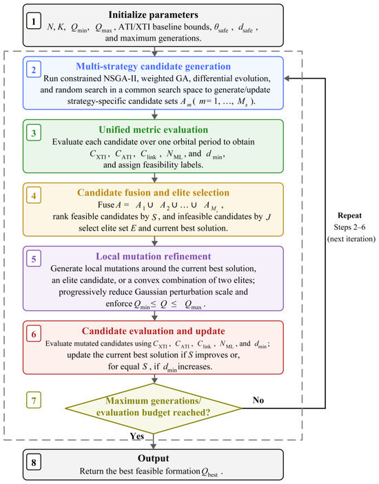
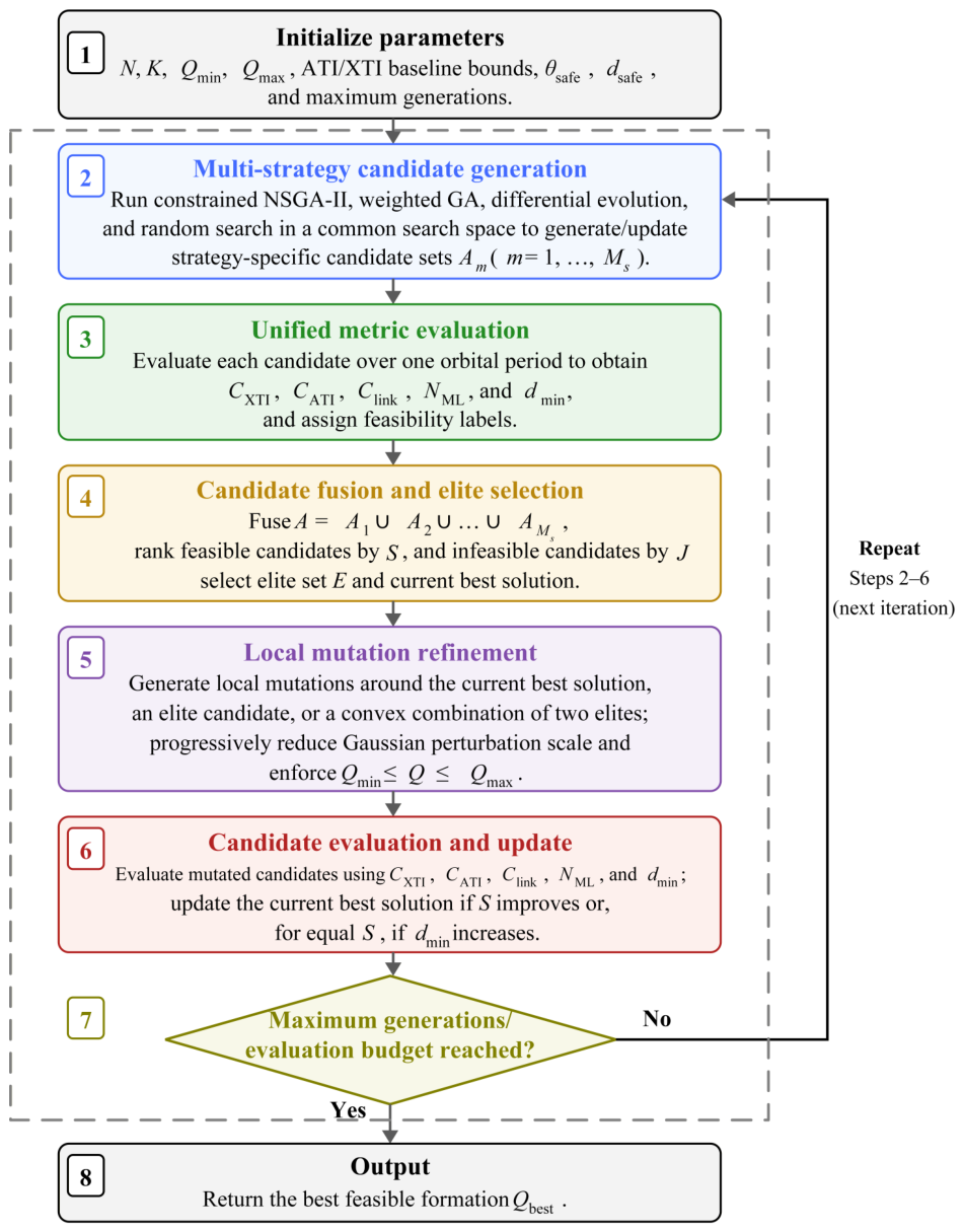
During local mutation refinement, the mutation base is selected from the current best solution, an elite solution, or a convex combination of two elites, and zero-mean Gaussian perturbations are added within the allowable range of each design variable. The perturbation scale is progressively reduced during refinement. Mutated variables are clipped to their bounds and reevaluated using the same metrics and hard constraints. The current best solution is updated only when the composite score improves, or, for equal scores, when the minimum intersatellite separation increases. The MSCE search procedure for mainlobe-safe candidate formations is illustrated in Figure 2.

Figure 2. Flowchart of the MSCE framework for mainlobe-safe candidate formation search.

Through the above mechanism, MSCE jointly exploits the multiobjective diversity of constrained NSGA-II, the focused exploitation provided by the weighted GA, the continuous-variable exploration capability of differential evolution, and the additional feasible-region coverage provided by random search. The post-fusion local mutation stage further explores the neighborhoods of elite solutions. This cooperative mechanism reduces sensitivity to any single algorithm, initialization, or local optimum and improves the robustness of the mainlobe-safe formation search and the quality of the final feasible solution under complex constraints.

3.5. Mainlobe-Safe Single-Module Formation Optimization

Single-module optimization forms the basis of MSMFO. For a module containing $n_u$ satellites, one satellite is selected as the module-center satellite and the remaining $n_u-1$ satellites serve as auxiliary satellites. The objective is to improve ATI/XTI baseline compliance and synchronization-link availability while satisfying mainlobe-safety and minimum-separation constraints.

For single-module optimization, the set of satellite pairs included in baseline evaluation is defined as

$${\mathcal{P}}_b^{\mathrm{unit}}=\{\left(1,\ell \right)\mid \ell =2,3,\dots ,n_u\},$$

(37)

where local index 1 denotes the module-center satellite and $\ell =2,\dots ,n_u$ denotes an auxiliary satellite within the module.

The single-module optimization problem is formulated as

$$\underset{{\mathbf{Q}}^{\mathrm{unit}}}{max}\left[\begin{array}{c}{C}_{\mathrm{XTI}}^{\mathrm{unit}}\hfill \\ C_{\mathrm{ATI}}^{\mathrm{unit}}\hfill \\ C_{\mathrm{link}}^{\mathrm{unit}}\hfill \end{array}\right]$$

(38)

subject to

$$\left\{\begin{array}{c}{N}_{\mathrm{ML}}^{\mathrm{unit}}=0,\hfill \\ d_{min}^{\mathrm{unit}}\ge d_{\mathrm{safe}},\hfill \\ {\mathbf{Q}}_{min}^{\mathrm{unit}}\le {\mathbf{Q}}^{\mathrm{unit}}\le {\mathbf{Q}}_{max}^{\mathrm{unit}}.\hfill \end{array}\right.$$

(39)

where $C_{\mathrm{XTI}}^{\mathrm{unit}}$ and $C_{\mathrm{ATI}}^{\mathrm{unit}}$ are the intramodule XTI and ATI baseline compliance rates, respectively; $C_{\mathrm{link}}^{\mathrm{unit}}$ is the intramodule synchronization-link availability; $N_{\mathrm{ML}}^{\mathrm{unit}}$ is the total number of intramodule mainlobe conflicts; and $d_{\min }^{\mathrm{unit}}$ is the minimum intramodule intersatellite separation.

During optimization, MSCE generates and updates the design vectors, while MSMFO maps each design vector to a candidate module geometry and evaluates its mission performance and safety. A candidate is declared infeasible if any mainlobe conflict occurs or if the intersatellite separation falls below the prescribed minimum. The feasible module with the highest composite score is finally selected as the basic module and used as the local formation template for subsequent scaling to a large-scale MuSAR formation.

The single-module optimization mechanism is reusable across formation scales. For a given module size and set of local mission requirements, the module-layer geometry needs to be optimized only once; the resulting module can then serve as a reusable local template at different module centers, with only module-dependent phase and offset adjustments introduced when necessary. In the simulations of Section 4, the six-satellite case is used to validate the single-module optimization mechanism and to support comparisons among optimization strategies and classical formations, whereas the eight-satellite module used in the 96-satellite simulation is independently optimized once using the same mechanism.

3.6. Two-Level Center-Layer/Module-Layer Modular Formation Design

For a large-scale MuSAR formation with dozens to nearly one hundred satellites, directly including all relative-motion parameters in a single global optimization causes the number of design variables to grow approximately linearly with satellite count, while intersatellite mainlobe-conflict and minimum-separation checks involve all satellite pairs and therefore scale approximately quadratically with satellite count. To reduce optimization difficulty and improve the organization of the formation architecture, a two-level center-layer/module-layer modular design is proposed.

Assume that the large-scale MuSAR formation consists of M modules, each containing $n_u$ satellites. The total number of satellites is

$$N=M{n}_u.$$

(40)

For module m, a satellite with local index ℓ corresponds to global satellite number $(m-1)n_u+\ell$. The module-center satellite therefore has global number $(m-1)n_u+1$.

The two-level modular design decomposes formation optimization into two layers. The first layer is the center-layer design, in which each module is treated as an equivalent node and the long-baseline relative motion among module centers is optimized. The center-layer design variables are denoted by $Q_{\mathrm{center}}$. The main objective is to generate observation geometries among module centers that satisfy the prescribed long-baseline XTI/ATI baseline ranges while avoiding intersatellite mainlobe conflicts and unsafe close approaches between module centers. The second layer is the module-layer design, in which auxiliary satellites are arranged around each module-center satellite to form a local cooperative observation unit. Its objective is to obtain high local ATI/XTI baseline compliance rates while satisfying intramodule mainlobe safety and minimum-separation constraints.

Accordingly, both the center-layer and module-layer designs reuse the same single-module optimization mechanism and are solved using MSCE, although they operate at different spatial scales and employ different baseline requirements. The optimized module-layer geometry is then replicated across the module centers, with module-dependent phase and offset corrections applied only when required by the global constraints.

The center-layer optimization problem is formulated as

$$\underset{{\mathbf{Q}}^{\mathrm{center}}}{max}\left[\begin{array}{c}{C}_{\mathrm{XTI}}^{\mathrm{center}}\hfill \\ C_{\mathrm{ATI}}^{\mathrm{center}}\hfill \\ C_{\mathrm{link}}^{\mathrm{center}}\hfill \end{array}\right]$$

(41)

subject to

$$\left\{\begin{array}{c}{N}_{\mathrm{ML}}^{\mathrm{center}}=0,\hfill \\ d_{min}^{\mathrm{center}}\ge d_{\mathrm{safe}},\hfill \\ {\mathbf{Q}}_{min}^{\mathrm{center}}\le {\mathbf{Q}}^{\mathrm{center}}\le {\mathbf{Q}}_{max}^{\mathrm{center}}.\hfill \end{array}\right.$$

(42)

After the center-layer and module-layer geometries have been designed, a global consistency check is required. Although each layer may individually satisfy its local constraints, satellites belonging to different modules may still experience intersatellite mainlobe conflicts or unsafe close approaches at certain sampling instants. Therefore, $N_{\mathrm{ML}}^{\mathrm{global}}$ and $d_{\min }^{\mathrm{global}}$ must be recomputed over the complete formation, and the final formation must satisfy

$$N_{\mathrm{ML}}^{\mathrm{global}}=0,$$

(43)

$$d_{min}^{\mathrm{global}}\ge d_{\mathrm{safe}}.$$

(44)

where $N_{\mathrm{ML}}^{\mathrm{global}}$ denotes the total number of global mainlobe conflicts during one orbital period, and $d_{\min }^{\mathrm{global}}$ denotes the minimum intersatellite separation among all satellite pairs over all sampled time instants. If the global check fails, the module-center phases, module-layer phase offsets, or mean along-track offsets should be adjusted, followed by a new round of global verification.

Let the phase offset of the m-th module be ${\phi }_m$. The phase parameter of the i-th auxiliary satellite within that module can then be adjusted as

$${\theta }_{m,i}={\theta }_i+{\phi }_m.$$

(45)

If necessary, the cross-track phase offset and mean along-track offset can also be slightly adjusted:

$${\alpha }_{m,i}={\alpha }_i+\Delta {\alpha }_m,$$

(46)

$$l_{m,i}=l_i+\Delta l_m.$$

(47)

where $\Delta {\alpha }_m$ and $\Delta l_m$ denote, respectively, the cross-track phase correction and along-track offset correction for the m-th module.

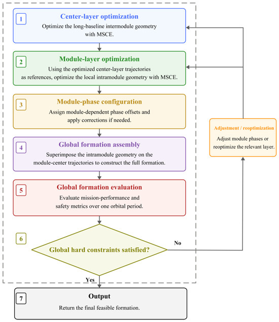
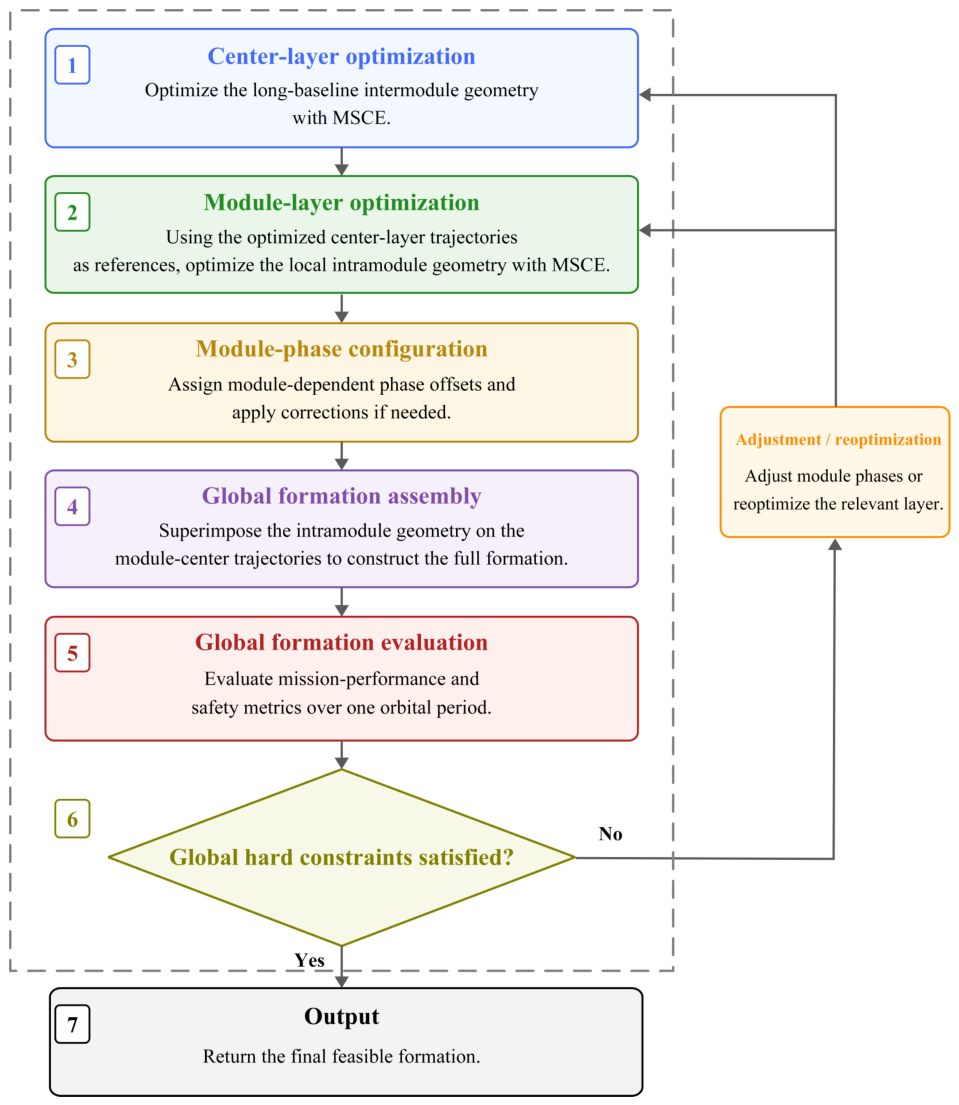
The large-scale MuSAR formation design and global-validation workflow of MSMFO is illustrated in Figure 3.

Figure 3. MSMFO workflow for large-scale MuSAR formation design and global validation.

With this hierarchical generation and global-validation mechanism, MSMFO does not optimize all satellites simultaneously in a single global problem. Instead, it first determines the long-baseline geometry among module centers, then optimizes the local module geometry around each center, and finally performs a global safety check. This sequence reduces the optimization dimensionality, allows the long-baseline mission geometry to explicitly constrain local module placement, improves design interpretability, and facilitates scaling the number of modules according to mission requirements.

4. Simulation Setup and Results

This section systematically evaluates the proposed MSMFO method through four groups of numerical simulations: single-module optimization, optimization-strategy comparison, comparison with classical formations, and modular scaling to a large-scale MuSAR formation. These simulations address three questions: (1) whether the proposed method can obtain feasible formations with balanced ATI/XTI baseline performance under hard constraints on intersatellite mainlobe conflicts and intersatellite separation; (2) whether MSCE improves the quality of the final solution relative to individual optimization strategies; and (3) whether the two-level center-layer/module-layer design can scale the formation to 96 satellites while maintaining ATI/XTI baseline performance and global safety.

4.1. Simulation Setup and Evaluation Metrics

The orbit-propagation model includes the J2 perturbation associated with Earth’s nonspherical gravity field. The reference orbit is a near-circular orbit, whose initial orbital parameters are listed in Table 1.

Table 1. Reference-orbit parameters.

Parameter	Value
Semimajor axis	6978.074 km
Eccentricity	0.001
Inclination	97.4
Right ascension of the ascending node	340.571°
Argument of perigee	90.019°
Mean anomaly	89.981°
Orbital period	5801.154 s

The simulated formations use the parameterized relative-motion model defined in Section 2. The baseline compliance rate measures the fraction of evaluated baselines that fall within the prescribed window over one orbital period. Only satellite pairs that actually participate in cooperative imaging are included in this statistic; satellite pairs not assigned to cooperative imaging are excluded from the average. Synchronization-link availability denotes the fraction of the orbital period for which the synchronization links satisfy the geometric-clearance condition.

A single-transmitter/multiple-receiver operating mode is assumed. Within each module, only the central satellite transmits radar signals, while the remaining satellites receive the ground echoes. The radar uses right-looking broadside geometry with a 45° look angle, a 4° mainlobe half-angle, and a 2° safety margin. Intersatellite mainlobe conflicts and intersatellite separation are treated as hard constraints, whereas synchronization-link availability is included as a soft performance metric. The main mission parameters and optimization settings are given in Table 2.

Table 2. Main mission parameters and optimization settings.

Parameter	Value	Applicability
Single-module satellite count	6	Single-module simulation
Scalability-study formation sizes	8, 24, 48, 72, and 96 satellites	Scalability study
Intramodule XTI baseline window	600–1900 m	Module layer
Intramodule ATI baseline window	500–2100 m	Module layer
Center-layer XTI/ATI baseline window	3–40 km	Center layer
Minimum intersatellite separation	150 m	All simulations
Mainlobe half-angle/safety margin	4°/2°	All simulations
Synchronization-link clearance threshold	10 m	All simulations
Population size/number of generations	36/20	All simulations

The 45° look angle is used to construct the LOS and range-plane perpendicular unit vectors for the effective perpendicular-baseline calculation and is also used in the intersatellite mainlobe-safety check.

4.2. Single-Module Mainlobe-Safe Formation Optimization

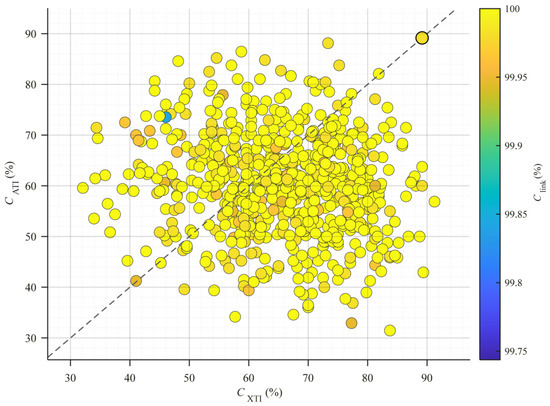
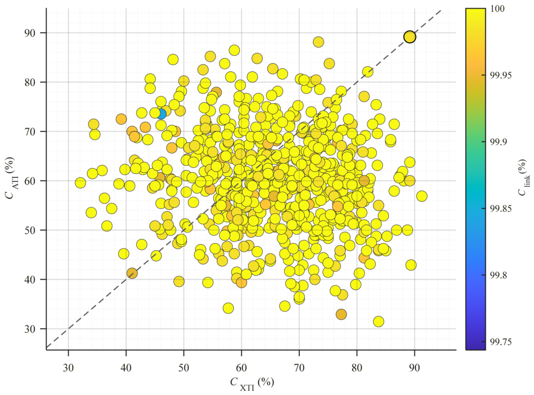
A single module comprising six satellites is first optimized. The strategy-specific candidate sets are evaluated using the same metrics and hard constraints and then combined into the pooled MSCE candidate set $A=A_1\cup A_2\cup \cdots \cup A_{M_s}$. Figure 4 provides a two-dimensional visualization of the sampled candidate distribution in terms of XTI and ATI compliance rather than an exhaustive record of every candidate in A. Color denotes synchronization-link availability, and the circular marker with a black edge indicates the final feasible solution obtained after candidate fusion, elite selection, and local mutation refinement.

Figure 4. Distribution of evaluated candidate formations from the pooled MSCE candidate set and the final feasible solution obtained after candidate fusion and local mutation refinement. The dashed diagonal line indicates equal XTI and ATI compliance.

Figure 4 is used to illustrate the distribution of the evaluated candidates and the position of the final solution. The sampled candidates exhibit different XTI/ATI balance characteristics, whereas the selected formation lies in the high-XTI, high-ATI region, with both baseline compliance rates equal to 89.17%, indicating no pronounced directional bias between the two observation tasks.

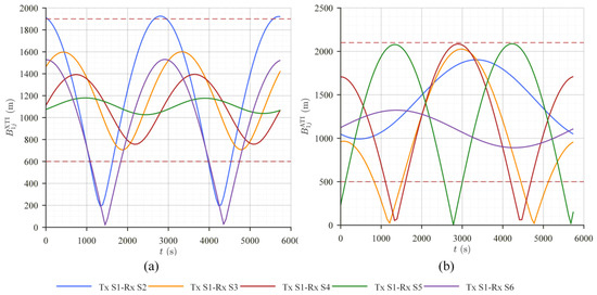
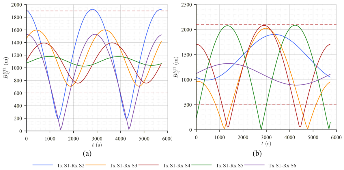
Figure 5 shows the variations in the XTI and ATI baselines of the final formation over one orbital period. Curves with different colors correspond to transmitter–receiver pairs formed by the central transmitting satellite and the individual receiving satellites; the same color denotes the same transmitter–receiver pair in the XTI and ATI subplots. Although some pairs leave the valid windows over limited intervals, the orbital-period XTI and ATI baseline compliance rates both remain 89.17%.

Figure 5. Baseline variations of the optimized single-module formation. (a) XTI baseline. (b) ATI baseline. The red dashed lines indicate the prescribed baseline bounds.

The same five transmitter–receiver pairs, ${\mathcal{P}}_b^{\mathrm{unit}}=\{(1,\ell )\mid \ell =2,\dots ,6\}$, are used to evaluate both ATI and XTI performance; no separate satellite subsets are assigned to the two tasks. The simultaneous joint compliance rate of 78.33% therefore represents the pair-time samples for which the same pair satisfies both baseline requirements at the same instant. The joint availability of 100.00% means that, at every sampled instant, at least one of the five pairs satisfies both requirements simultaneously, so no sampled joint-task gap occurs over the orbital period.

Table 3 further shows that the final formation has identical XTI and ATI baseline compliance rates, avoiding a strong bias toward either observation direction. Synchronization-link availability reaches 99.98%, while both the number of mainlobe conflicts and the number of events with separation below 150 m are zero. In addition, the complete set of orbital parameters for the optimized single-module formation is provided in Appendix A. The reported baseline performance is therefore achieved within the feasible region defined by the hard constraints rather than by relaxing the safety requirements.

Table 3. Single-module optimization results.

Metric	Value
XTI baseline compliance rate	89.17%
ATI baseline compliance rate	89.17%
Simultaneous joint compliance rate	78.33%
Joint availability	100.00%
Synchronization-link availability	99.98%
Mainlobe-conflict count	0
Minimum-separation violation count	0

4.3. Comparison of Optimization Strategies

To assess the role of MSCE, it is compared under identical conditions with constrained NSGA-II, a weighted GA, differential evolution, and random search. The four individual strategies first generate candidate solutions independently using the same search space, orbital model, and constraints. MSCE then pools the candidate solutions obtained from these strategies, applies the unified feasibility and ranking rules defined in Section 3.3, performs local refinement around high-quality feasible candidates, and selects the final solution.

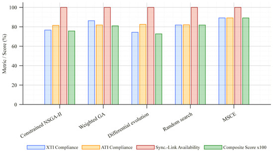
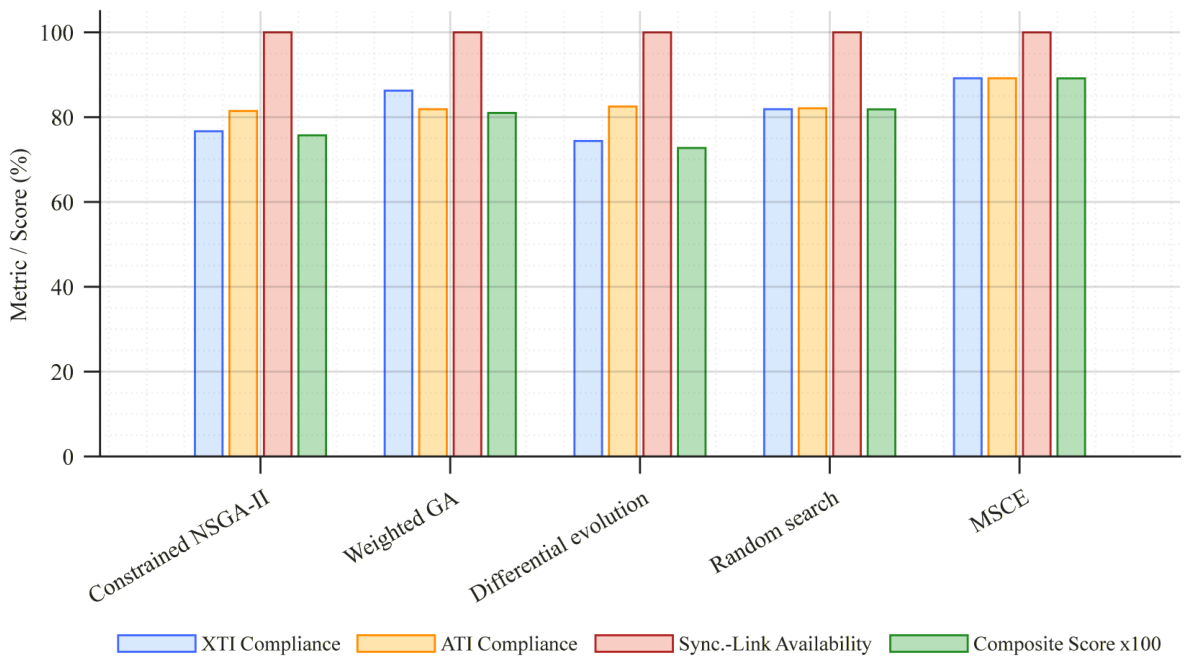
Table 4 and Figure 6 show that random search achieves the highest score among the four individual strategies, 0.8183, but the smaller of its XTI and ATI compliance rates is 81.87%. After feasible-elite fusion and local refinement, MSCE increases both compliance rates to 89.17% and raises the composite score to 0.8915. This corresponds to an absolute score increase of 0.0732, or approximately 8.9%, relative to the best individual strategy, while the minimum of the two baseline compliance rates increases by 7.30 percentage points.

Table 4. Performance comparison of different optimization strategies.

Strategy	XTI Compliance (%)	ATI Compliance (%)	Sync.-Link Availability (%)	ML Conflict Count	Separation Violations	Feasible	Composite Score
Constrained NSGA-II	76.67	81.46	100.00	0	0	Yes	0.7571
Weighted GA	86.25	81.87	100.00	0	0	Yes	0.8099
Differential evolution	74.38	82.50	99.98	0	0	Yes	0.7274
Random search	81.87	82.08	100.00	0	0	Yes	0.8183
MSCE	89.17	89.17	99.98	0	0	Yes	0.8915

Figure 6. Comparison of best-solution metrics and composite scores for different optimization strategies.

These results indicate that the advantage of MSCE does not lie in maximizing a single metric. Rather, it exploits the complementary exploration behavior of different search strategies in a nonconvex feasible region and uses local refinement to further reduce directional bias between XTI and ATI performance. Consequently, MSCE yields formations with more balanced XTI/ATI baseline compliance and a higher composite score while satisfying all hard constraints.

4.4. Comparison with Classical Formations

To evaluate the advantages of the proposed method over classical formations, MSMFO is compared with cartwheel, pendulum, and helix formations [16] using the same six-satellite configuration, orbital propagation model, mission-required baseline windows, and safety criteria.

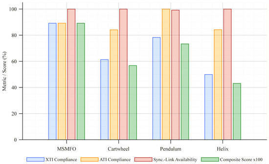
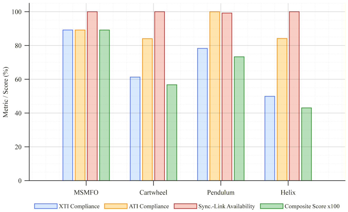
Table 5 shows that the cartwheel formation satisfies the mainlobe safety and minimum-separation constraints, but its XTI and ATI baseline compliance rates are 61.30% and 84.07%, respectively, indicating a pronounced imbalance between XTI and ATI compliance. The pendulum formation achieves 100.00% ATI compliance but only 78.28% XTI compliance. The helix formation provides 100.00% synchronization-link availability and has no minimum-separation violation, but it produces 68 mainlobe-conflict occurrences accumulated over directed satellite pairs and sampled time instants according to Equation (25); this value does not represent 68 independent continuous-time conflict events. Because mainlobe exclusion is imposed as a hard constraint, the positive occurrence count makes the helix formation infeasible. Figure 7 compares the performance metrics and composite scores of MSMFO and the classical formations for the same satellite count. These results indicate that satisfying the minimum separation requirement does not imply geometric safety with respect to the radar mainlobe; intersatellite mainlobe conflicts must be explicitly incorporated into formation design.

Table 5. Performance comparison between MSMFO and classical formations.

Formation	XTI Compliance (%)	ATI Compliance (%)	Sync.-Link Availability (%)	ML Conflict Count	Separation Violations	Feasible	Composite Score
MSMFO	89.17	89.17	99.98	0	0	Yes	0.8915
Cartwheel	61.30	84.07	100.00	0	0	Yes	0.5675
Pendulum	78.28	100.00	99.19	0	0	Yes	0.7330
Helix	49.91	84.17	100.00	68	0	No	0.4306

Figure 7. Comparison of performance metrics and composite scores between MSMFO and classical formations with the same satellite count.

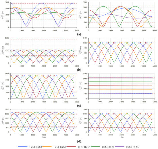
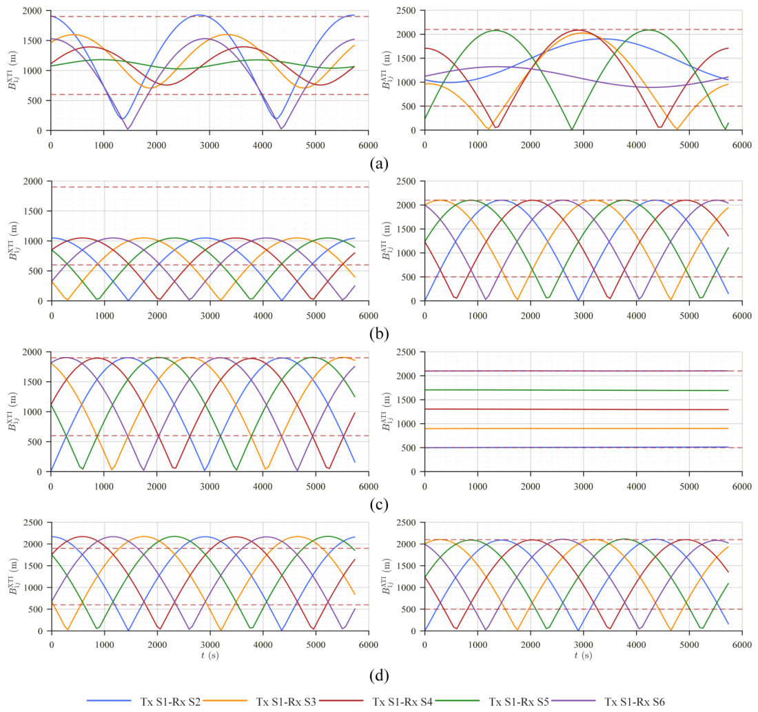
With zero mainlobe conflicts and zero minimum separation violations, MSMFO achieves XTI and ATI baseline compliance rates of 89.17% simultaneously. If the smaller of the two compliance rates is used as a conservative measure of mission performance, the best feasible classical formation is the pendulum formation, with a minimum compliance rate of 78.28%. MSMFO increases this value by 10.89 percentage points, corresponding to a relative increase of approximately 13.9%. Under the same composite scoring criterion as in Table 4, MSMFO obtains a score of 0.8915, compared with 0.7330 for the pendulum, 0.5675 for the cartwheel, and 0.4306 for the helix. Figure 8 shows the XTI/ATI baseline variations of the evaluated satellite pairs for MSMFO and the classical formations. The orbital parameters of all satellites in both the MSMFO and classical formations are provided in Appendix A.

Figure 8. XTI/ATI baseline variations of the evaluated satellite pairs for MSMFO and classical formations. (a) MSMFO. (b) Cartwheel. (c) Pendulum. (d) Helix. The red dashed lines indicate the prescribed baseline bounds.

These results show that the proposed method mitigates the directional limitations of classical formations through joint optimization of relative-motion amplitudes, phases, and along-track offsets, thereby obtaining more balanced XTI/ATI baseline compliance while satisfying the safety constraints.

4.5. Sensitivity Analysis of Key Parameters

A sensitivity analysis was conducted using the six-satellite formation to examine the effects of the mainlobe half-angle, angular safety margin, baseline-window width, and minimum intersatellite distance. In addition to the XTI and ATI compliance rates, the balanced compliance rate $min\left(C_{\mathrm{XTI}},C_{\mathrm{ATI}}\right)$, the simultaneous joint compliance rate $C_{\mathrm{joint}}$, the joint availability $A_{\mathrm{joint}}$, and the feasible-candidate fraction were considered. The first three metrics are defined in Section 2.3, whereas the feasible-candidate fraction denotes the proportion of evaluated candidate formations that satisfy all hard safety constraints.

Because the mainlobe half-angle and angular safety margin jointly determine the angular threshold through ${\theta }_{\mathrm{safe}}={\theta }_{\mathrm{ML}}+{\theta }_{\mathrm{margin}}$, their combined influence was evaluated through the full angular safety range. Five full angular safety ranges of ${10}^{°}$, ${15}^{°}$, ${20}^{°}$, ${25}^{°}$, and ${30}^{°}$ were considered. As the full angular safety range increased from ${10}^{°}$ to ${30}^{°}$, the mean balanced XTI/ATI compliance rate decreased from 82.43% to 78.47%, the joint compliance rate decreased from 66.18% to 60.21%, and the feasible-candidate fraction decreased monotonically from 33.33% to 14.40%. Thus, a stricter angular safety requirement progressively contracts the feasible formation-design space and eventually reduces the achievable task performance.

The influence of the minimum intersatellite distance was evaluated by increasing the threshold from 150 to 750 m. The feasible-candidate fraction decreased monotonically from 33.33% at 150 m to 24.28%, 15.14%, 8.49%, and 0.83% as the threshold increased. For thresholds from 150 to 600 m, reoptimization maintained comparable XTI and ATI performance, indicating that the proposed method can accommodate a moderate tightening of the separation constraint. At 750 m, however, the mean XTI, ATI, and joint compliance rates decreased to 73.82%, 65.56%, and 48.54%, respectively. An excessively restrictive separation requirement therefore substantially reduces the feasible design space and can cause a clear loss of mission performance.

Sensitivity to the baseline-window width was evaluated by scaling the nominal XTI and ATI windows. When the windows were reduced to 0.75 times their nominal widths, the XTI, ATI, and joint compliance rates decreased to 78.75%, 71.88%, and 51.88%, respectively, and the joint availability decreased to 82.29%. Under the nominal windows, the corresponding values were 89.17%, 89.17%, 78.33%, and 100%. When the windows were increased to 1.25 times their nominal widths, the XTI, ATI, and joint compliance rates increased to 93.75%, 93.33%, and 87.08%, respectively, while the joint availability remained 100%. The baseline-window specification therefore directly affects both achievable task compliance and the temporal continuity of simultaneous ATI/XTI observations. It should be noted that the baseline window should be designed according to the mission performance requirements.

Overall, the sensitivity analysis shows a clear tradeoff between task performance and constraint strictness. Increasing the angular safety requirement or the minimum intersatellite distance restricts the feasible formation-design space, whereas the baseline-window width directly affects achievable ATI/XTI compliance and joint task availability. These results provide a quantitative reference for practical parameter selection within the same MSMFO optimization framework.

4.6. Multi-Scale Validation of the Modular Formation

To remove the confounding effect of different local designs, a controlled scalability study was conducted using the same eight-satellite module template for formations containing 8, 24, 48, 72, and 96 satellites, corresponding to 1, 3, 6, 9, and 12 modules, respectively. The module-layer and center-layer results are summarized in Table 6.

Table 6. Module-layer and center-layer performance at different formation sizes.

Satellites	Modules	Module XTI (%)	Module ATI (%)	Module joint (%)	Center XTI (%)	Center ATI (%)	Center Joint (%)
8	1	83.33	83.33	66.67	–	–	–
24	3	83.33	83.33	66.67	100.00	100.00	100.00
48	6	83.33	83.33	66.67	98.52	96.30	95.00
72	9	83.33	83.33	66.67	95.91	92.82	88.73
96	12	83.33	83.33	66.67	91.79	91.41	83.21

All tested multi-module formations achieved 100% simultaneous joint availability and 100% synchronization-link availability, with no global mainlobe conflict or minimum-separation violation. The center-layer compliance decreases gradually as the number of modules increases, whereas the fixed module-layer performance remains unchanged. This controlled comparison therefore separates the effect of increasing formation size from differences between local module designs.

Table 7 shows that center-layer optimization and full-formation candidate screening account for most of the computational cost. For all tested formation sizes, the final global safety and synchronization-link evaluations together required less than 30 ms and therefore accounted for only a small fraction of the total computational cost.

Table 7. Computational cost at different formation sizes.

Number of Satellites	Center-Layer Optimization (s)	Full-Formation Screening (s)	Total Computation Time (s)
24	19.08	4.63	23.72
48	41.79	13.96	55.77
72	80.86	20.94	101.84
96	134.54	80.38	214.96

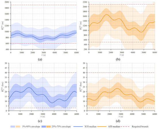
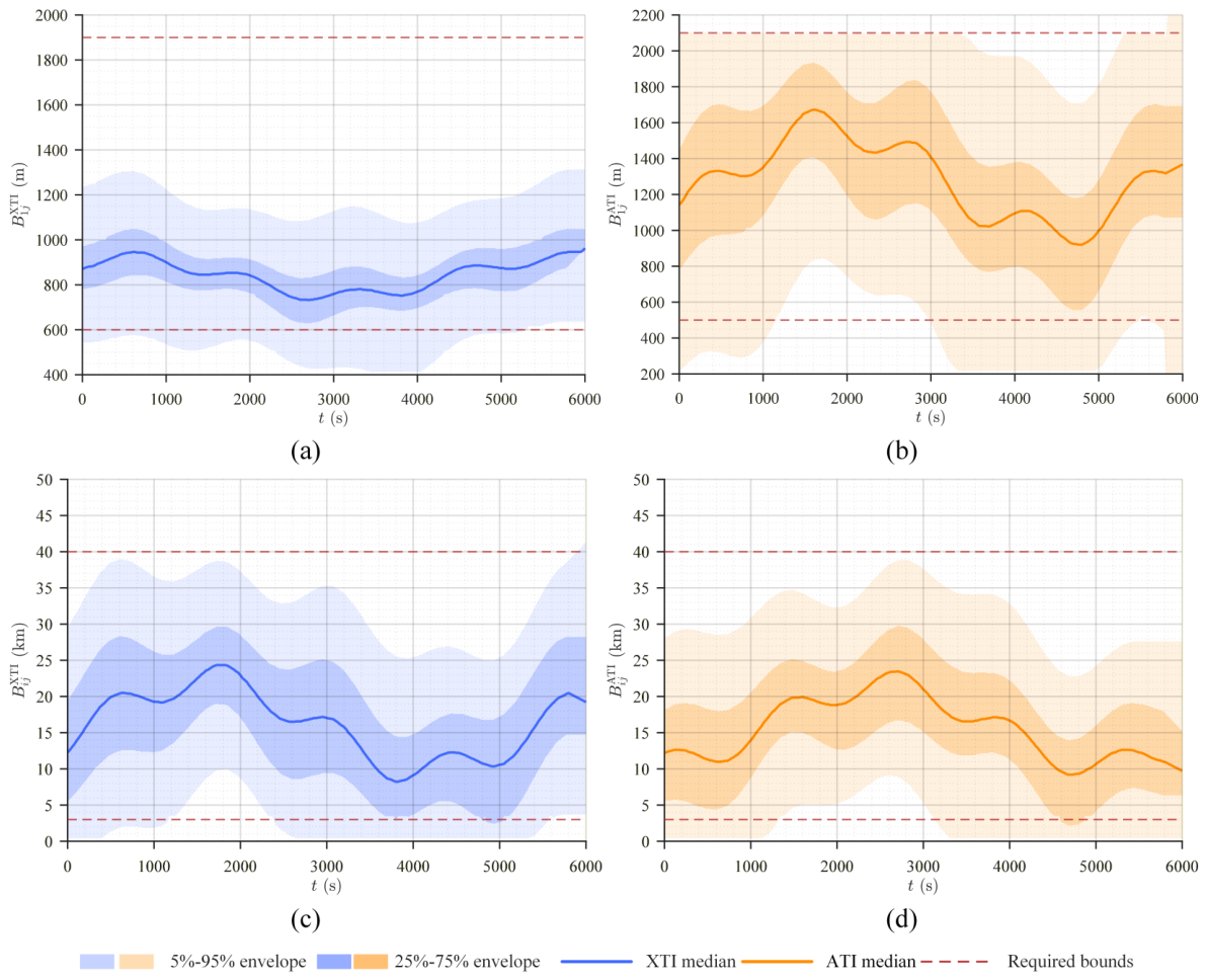
Taking the 96-satellite formation as an example, Figure 9 illustrates the temporal variations of its module-layer and center-layer baselines. The formation consists of 12 eight-satellite modules, yielding 84 intramodule task-pair curves ($7\times 12=84$, corresponding to seven evaluated task pairs per module) and 66 center-layer task-pair curves ($\left({\displaystyle \genfrac{}{}{0pt}{}{12}{2}}\right)=66$, corresponding to all pairwise combinations of the 12 module centers). To avoid visual clutter from overlapping these curves, the baseline variations are summarized using quantile envelopes. The light-shaded regions represent the 5th–95th percentile envelopes, the dark-shaded regions represent the 25th–75th percentile envelopes, and the solid lines denote the median. The horizontal dashed lines indicate the prescribed baseline windows. The center-layer orbital parameters of the 96-satellite formation and the orbital parameters of its first module are provided in Appendix A.

Figure 9. Quantile envelopes of module-layer and center-layer XTI/ATI baselines for the 96-satellite formation. (a) Module-layer XTI baselines. (b) Module-layer ATI baselines. (c) Center-layer XTI baselines. (d) Center-layer ATI baselines. The red dashed lines indicate the prescribed baseline bounds.

5. Discussion

It should be noted that this paper addresses mainlobe safety primarily from the perspective of geometric formation design. The current circular-cone and discretely sampled model does not replace measured antenna patterns, power-coupling analysis, receiver-threshold verification, continuous-time conflict detection, or onboard safety interlocks. Future work can extend the present framework by introducing higher-fidelity payload models and additional engineering constraints to further assess its practical applicability and robustness. Such extensions would enable robustness analysis under nonideal operating conditions and provide a closer connection between geometric formation design and payload-level engineering constraints.

Recent remote-sensing tracking studies also suggest two useful directions for future extensions. The spatial-temporal proximity and topological relationships used in satellite-video multi-target tracking [27] motivate topology-aware regularity measures for evaluating intramodule layouts and baseline distributions. Foreground-background motion compensation in Video-SAR tracking [28] suggests incorporating scene- or clutter-dependent observation-quality metrics as additional optimization objectives.

6. Conclusions

This paper proposes an MSMFO method for large-scale MuSAR formations with joint ATI/XTI baseline requirements. By integrating ATI/XTI baseline compliance, synchronization-link availability, intersatellite mainlobe conflicts, and minimum intersatellite separation into a unified optimization framework, MSMFO jointly addresses mission performance and safety constraints. The MSCE framework improves optimization performance under complex constraints, while the two-level center-layer/module-layer strategy enables modular scaling to formations comprising a large number of satellites.

Numerical simulations demonstrate the effectiveness and scalability of the proposed method. For the six-satellite module, MSMFO achieves XTI and ATI baseline compliance rates of 89.17% each, with 99.98% synchronization-link availability and no safety violations. Compared with the best individual optimization strategy, MSCE improves the composite score by approximately 8.9%. Compared with the best feasible classical formation, the lower of the XTI and ATI baseline compliance rates is improved by 10.89 percentage points. In the controlled 8–96-satellite study, the fixed eight-satellite module retains XTI and ATI compliance rates of 83.33%, while the center-layer XTI and ATI compliance rates remain 91.79% and 91.41%, respectively, at the 96-satellite scale. All tested multi-module formations achieve 100% joint and synchronization-link availability and produce no global mainlobe conflicts or minimum-separation violations. These results show that MSMFO provides a physically interpretable framework for mainlobe-safe large-scale MuSAR formation design and support its scalability through modular extension to large-scale formations.

References

- Moreira, A.; Prats-Iraola, P.; Younis, M.; Krieger, G.; Hajnsek, I.; Papathanassiou, K.P. A tutorial on synthetic aperture radar. IEEE Geosci. Remote Sens. Mag. 2013, 1, 6–43. [Google Scholar] [CrossRef] [Scilit]
- Krieger, G.; Moreira, A. Spaceborne bi- and multistatic SAR: Potential and challenges. IEE Proc.-Radar Sonar Navig. 2006, 153, 184–198. [Google Scholar] [CrossRef] [Scilit]
- Farr, T.G.; Rosen, P.A.; Caro, E.; Crippen, R.; Duren, R.; Hensley, S.; Kobrick, M.; Paller, M.; Rodriguez, E.; Roth, L.; et al. The Shuttle Radar Topography Mission. Rev. Geophys. 2007, 45, RG2004. [Google Scholar] [CrossRef] [Scilit]
- Krieger, G.; Moreira, A.; Fiedler, H.; Hajnsek, I.; Werner, M.; Younis, M.; Zink, M. TanDEM-X: A satellite formation for high-resolution SAR interferometry. IEEE Trans. Geosci. Remote Sens. 2007, 45, 3317–3341. [Google Scholar] [CrossRef] [Scilit]
- Lou, L.; Liu, Z.; Zhang, H.; Qian, F.; Huang, Y. TH-2 satellite engineering design and implementation. Acta Geod. Cartogr. Sin. 2020, 49, 1252–1264. [Google Scholar] [CrossRef]
- Wang, R.; Liu, K.; Liu, D.; Ou, N.; Yue, H.; Chen, Y.; Yu, W.; Liang, D.; Cai, Y. LuTan-1: An innovative L-band spaceborne bistatic interferometric synthetic aperture radar mission. IEEE Geosci. Remote Sens. Mag. 2025, 13, 58–78. [Google Scholar] [CrossRef] [Scilit]
- Deng, Y.; Zhang, H.; Liu, K.; Wang, W.; Ou, N.; Han, H.; Yang, R.; Ren, J.; Wang, J.; Ren, X.; et al. Hongtu-1: The first spaceborne single-pass multibaseline SAR interferometry mission. IEEE Trans. Geosci. Remote Sens. 2025, 63, 5202518. [Google Scholar] [CrossRef] [Scilit]
- Bartusch, M.; Nuncio Quiroz, A.E.; Stettner, S.; Moreira, A.; Zink, M. German X-band spaceborne SAR heritage and the future HRWS mission. In Proceedings of the 2021 IEEE International Geoscience and Remote Sensing Symposium (IGARSS), Brussels, Belgium, 11–16 July 2021; pp. 804–807. [Google Scholar] [CrossRef] [Scilit]
- Lopez-Dekker, P.; Rott, H.; Prats-Iraola, P.; Chapron, B.; Scipal, K.; De Witte, E. Harmony: An Earth Explorer 10 mission candidate to observe land, ice, and ocean surface dynamics. In Proceedings of the 2019 IEEE International Geoscience and Remote Sensing Symposium (IGARSS), Yokohama, Japan, 28 July–2 August 2019; pp. 8381–8384. [Google Scholar] [CrossRef] [Scilit]
- Dong, S.; Yu, W.; Wang, J.; Wu, Y.; Lin, Q.; Wang, C.; Jia, X. A single-pass multistatic SAR satellites formation design method for TomoSAR data acquisition. IEEE J. Sel. Top. Appl. Earth Obs. Remote Sens. 2026, 19, 19459–19475. [Google Scholar] [CrossRef] [Scilit]
- Wang, Z.; Yu, W.; Wang, J.; Xiang, W.; Liu, Y.; Wei, Y.; Guo, S.; Yang, R. Orthogonal complement subspace projection for hybrid baseline ocean current inversion. IEEE J. Sel. Top. Appl. Earth Obs. Remote Sens. 2026, 19, 26845–26859. [Google Scholar] [CrossRef] [Scilit]
- Kahle, R.; Schlepp, B.; Aida, S.; Kirschner, M.; Wermuth, M. Flight dynamics operations of the TanDEM-X formation. In Proceedings of the 12th International Conference on Space Operations (SpaceOps 2012), Stockholm, Sweden, 11–15 June 2012. [Google Scholar] [CrossRef] [Scilit]
- Krieger, G.; Zink, M.; Bachmann, M.; Bräutigam, B.; Schulze, D.; Martone, M.; Rizzoli, P.; Steinbrecher, U.; Antony, J.W.; De Zan, F.; et al. TanDEM-X: A radar interferometer with two formation-flying satellites. Acta Astronaut. 2013, 89, 83–98. [Google Scholar] [CrossRef] [Scilit]
- Zhang, Y.; Zhang, H.; Ou, N.; Liu, K.; Liang, D.; Deng, Y.; Wang, R. First demonstration of multipath effects on phase synchronization scheme for LT-1. IEEE Trans. Geosci. Remote Sens. 2020, 58, 2590–2604. [Google Scholar] [CrossRef] [Scilit]
- Sabol, C.; Burns, R.; McLaughlin, C.A. Satellite formation flying design and evolution. J. Spacecr. Rocket. 2001, 38, 270–278. [Google Scholar] [CrossRef] [Scilit] [PubMed]
- Zhang, Y.; Zhang, H.; Hou, S.; Deng, Y.; Yu, W.; Wang, R. An innovative superpolyhedron (SP) formation for multistatic SAR (M-SAR) interferometry. IEEE Trans. Geosci. Remote Sens. 2021, 59, 10136–10150. [Google Scholar] [CrossRef] [Scilit]
- Chen, Z.; Li, B.; Cai, Y.; Cao, S.; Lu, P.; Wang, R. A novel frequency-scanning (F-SCAN) phase synchronization scheme for bistatic/mutistatic SAR. IEEE Trans. Geosci. Remote Sens. 2025, 63, 5220716. [Google Scholar] [CrossRef] [Scilit]
- Clohessy, W.H.; Wiltshire, R.S. Terminal guidance system for satellite rendezvous. J. Aerosp. Sci. 1960, 27, 653–658. [Google Scholar] [CrossRef] [Scilit]
- Vallado, D.A. Fundamentals of Astrodynamics and Applications, 2nd ed.; Space Technology Library; Microcosm Press and Kluwer Academic Publishers: El Segundo, CA, USA; Dordrecht, The Netherlands, 2001; Volume 12. [Google Scholar]
- Liang, D.; Zhang, H.; Liu, K.; Liu, D.; Wang, R. Phase synchronization techniques for bistatic and multistatic synthetic aperture radar: Accounting for frequency offset. IEEE Geosci. Remote Sens. Mag. 2022, 10, 153–167. [Google Scholar] [CrossRef] [Scilit]
- Cai, Y.; Li, J.; Yang, Q.; Liang, D.; Liu, K.; Zhang, H.; Lu, P.; Wang, R. First demonstration of RFI mitigation in the phase synchronization of LT-1 bistatic SAR. IEEE Trans. Geosci. Remote Sens. 2023, 61, 5217319. [Google Scholar] [CrossRef] [Scilit]
- Jin, G.; Liu, K.; Liu, D.; Liang, D.; Zhang, H.; Ou, N.; Zhang, Y.; Deng, Y.; Li, C.; Wang, R. An advanced phase synchronization scheme for LT-1. IEEE Trans. Geosci. Remote Sens. 2020, 58, 1735–1746. [Google Scholar] [CrossRef]
- Deb, K.; Pratap, A.; Agarwal, S.; Meyarivan, T. A fast and elitist multiobjective genetic algorithm: NSGA-II. IEEE Trans. Evol. Comput. 2002, 6, 182–197. [Google Scholar] [CrossRef] [Scilit]
- Goldberg, D.E. Genetic Algorithms in Search, Optimization, and Machine Learning; Addison-Wesley: Reading, MA, USA, 1989. [Google Scholar]
- Storn, R.; Price, K. Differential evolution—A simple and efficient heuristic for global optimization over continuous spaces. J. Glob. Optim. 1997, 11, 341–359. [Google Scholar] [CrossRef] [Scilit]
- Solis, F.J.; Wets, R.J.B. Minimization by random search techniques. Math. Oper. Res. 1981, 6, 19–30. [Google Scholar] [CrossRef] [Scilit]
- Hong, J.; Wang, T.; Han, Y.; Wei, T. Multi-target tracking for satellite videos guided by spatial-temporal proximity and topological relationships. IEEE Trans. Geosci. Remote Sens. 2025, 63, 5614020. [Google Scholar] [CrossRef] [Scilit]
- Hong, J.; Wang, T.; Han, Y.; Di, W.; Dong, T. A multivehicle tracking method for Video-SAR with reliable foreground–background motion feature compensation. IEEE Trans. Geosci. Remote Sens. 2025, 63, 5207222. [Google Scholar] [CrossRef] [Scilit]
Disclaimer/Publisher’s Note: The statements, opinions and data contained in all publications are solely those of the individual author(s) and contributor(s) and not of MDPI and/or the editor(s). MDPI and/or the editor(s) disclaim responsibility for any injury to people or property resulting from any ideas, methods, instructions or products referred to in the content. |
© 2026 by the authors. Licensee MDPI, Basel, Switzerland. This article is an open access article distributed under the terms and conditions of the Creative Commons Attribution (CC BY) license.