


Highlights
What are the main findings?
- The WPS (Weighted Photon Spread) model was extended to natively support RAMI actual scene descriptions for radiative transfer (RT) simulation by representing the 3D canopies with the instancing technique at hierarchical levels and by analytically intersecting rays with spheres, cylinders, and cone frusta and their transformed forms, so that the original scene geometry is preserved without tessellation.
- Evaluations through ROMC (Radiation transfer model intercomparison Online Model Checker) and comparisons with a well-established RT model show that the extended WPS model is highly accurate for the simulation of photon transport in a 3D plant canopy.
What are the implications of the main findings?
- Adoption of the native RAMI scene descriptions as truthfully as possible removes the tessellation-related degree of freedom from the simulation and thereby eliminates one uncontrolled source of divergence among RT models over 3D canopy scenarios.
- Different representation methods may lead to the high divergences for RT simulations over the four RAMI-V actual scenarios among the participating Monte Carlo ray-tracing models.
Abstract
Radiative transfer (RT) models of vegetation canopy serve as powerful tools for the quantitative interpretation of remotely sensed signals. Based on the Monte Carlo ray-tracing (MCRT) model, WPS (Weighted Photon Spread), we performed extensions with new functionalities to better adapt the three-dimensional (3D) scenarios in the Radiation Transfer Model Intercomparison (RAMI) exercise. In terms of 3D canopy representation, the two most recent phases of the RAMI exercise (RAMI-IV/V) addressed two features: (1) extensive use of the instancing technique, where an individual component serves as a prototype, and its copies are transformed to generate an entire tree’s foliage; and (2) new scene definitions with more geometric primitives alongside flat objects like disks and triangles, e.g., spheres, cylinders, and cone frusta, and the utilization of transformations of these geometric primitives to describe actual scenes. New extensions were implemented in WPS to represent the 3D canopies with the instancing technique at hierarchical levels and to handle ray intersection for different geometric primitives and their transformed forms. Two new modes were therefore developed: WPS3INS, based on a two-layer axis-aligned bounding-box structure, and WPS3BVH, based on a bounding volume hierarchy that stores each transformation only once. Because spheres, cylinders, and cone frusta are intersected analytically and are never tessellated into triangles, every scene component of the RAMI-V actual scenarios is ray-traced at its native per-primitive fidelity, meaning that no geometric uncertainty of tessellation origin is introduced into the RT simulation. The extensions also deliver large memory savings: for the birch stand winter scene (HET15_JBS_WIN), which contains 138,251,607 primitives, WPS3BVH reduces the runtime memory by a factor of about 57 compared with WPS3. Evaluations through ROMC (Radiation transfer model intercomparison Online Model Checker) show that the accuracy of the new modes for 3D structure representation is within ±1% of the reference solution. Comparisons with the LESS model for selected RAMI-V actual canopy scenarios also show close agreement, with the lowest R2 of 0.999 and highest Relative Root Mean Square Error of ~1.553%. Future work based on the extended WPS model is suggested for the exploration of high divergences of RT simulations from the RAMI-V actual scenarios among the participating MCRT models.
1. Introduction
Radiative transfer (RT) models of the vegetation canopy are an essential component for the quantitative interpretation of remotely sensed signals. RT models quantitatively describe the absorption and scattering of solar energy by vegetative components [1]. Quantitative retrieval of biophysical and structural information from remote sensing (RS) data relies on the performance of both the RT model and the instruments used. Various RT models have been developed concurrently with emerging satellite RS techniques [2]. Among them, Monte Carlo ray-tracing (MCRT) models offer a simple, flexible, yet rigorous approach to the modeling of photon transport in a plant canopy, which can simultaneously calculate multiple physical quantities, such as albedo, radiant energy distribution within the canopy, bidirectional reflectance factor (BRF), and fraction of absorbed photosynthetically active radiation by vegetation [3,4]. With ever-increasing computational power and innovative variance reduction methods, three-dimensional (3D) MCRT simulation becomes more attractive for the development of RT modeling tools.
The complexity of 3D vegetation structure requires abstraction and simplification with different levels of detail in the description of the architecture of vegetation canopies used in RT models. The validation of RT models, especially MCRT models with detailed descriptions of 3D canopy structures and components’ spectral properties as inputs, requires time-consuming in situ measurements of canopy structure and radiometric characteristics. Indeed, it is not an easy task to completely validate one or another RT model with in situ measurements by considering the ever-changing and uncontrollable experimental conditions. However, the principles behind all RT models to solve light propagation in a medium are all based on the radiative transfer equation [5]. Under similar input conditions, different RT models should produce consistent RT simulations, which is one of the prime motivations for the Radiation Transfer Model Intercomparison (RAMI) exercise [6]. RAMI was designed to measure the variability between RT models, to document their accuracy and reliability in simulating well-controlled experimental conditions, and to provide diagnostics suitable to pinpoint possible deficiencies in these models [7]. Since the implementation of the first phase of RAMI (RAMI-I) [6], its continuous evolution up to the recently released results of RAMI-V has helped to document the uncertainties/errors among existing RT models and to establish a consensus among the surface RT modeling community for the identification of a set of credible models [8]. Partly as a result of RAMI exercises, the RAMI On-line Model Checker (ROMC) [9] enables RT model developers to verify the quality of their RT models against a reference for different canopy scenarios, which, at the time of writing, nevertheless contains only homogeneous and 3D abstract scenes. Within the RAMI-V exercise, four MCRT models, i.e., DART (Discrete Anisotropic Radiative Transfer model) [10,11], LESS (large-scale remote sensing data and image simulation framework over heterogeneous 3D scenes) [12], Raytran [4], and WPS (Weighted Photon Spread model) [13], could promisingly contribute to a new ROMC reference for four actual scenarios [8] (for more details, see Section 2.3.2).
With the evolvement of RAMI phases, the complexity of the scenes has increased, with more complex and realistic representations of canopy scenarios. Some new features on scene representations appeared in recent RAMI phases. For example, the instancing technique was extensively applied in RAMI-IV [14] and RAMI-V scenarios, especially those actual ones containing tens or hundreds of millions of primitives. Object instancing is a classic technique in computer graphics (CG) that reuses transformed copies of a single collection of geometries at multiple positions in a scene. If no corresponding scene description is designed in the MCRT models which read spatial information and spectral properties of all primitives into RAM (random-access memory) during runtime, performing RT simulations will incur a significant computational cost. Another feature is that more complex curved objects (spheres, cylinders, and frusta) alongside simpler flat objects (disks and triangles) were introduced in actual scenarios to achieve more realistic representation of the 3D canopy architecture. These new features bring about significant challenges for our WPS model, which was developed and has been maintained at Beihang University since 2012 (see more details about WPS in Section 2.2). To participate in the RAMI-V exercise, we extended the WPS model by addressing these new challenges.
Another motivation comes from the recent release of RAMI-V results: it is hard to define a benchmark (or credible reference MCRT model group) over two pine stand scenes and two realistic scenes defined through a semiparametric (Savanna) and an empirical (Wytham Woods) approach [8]. It was speculated that the high divergences arose mainly from different levels of detail in the description of the actual scenarios adopted by the participating MCRT models. However, there are no detailed references on how the RAMI-V actual scenarios were represented in the MCRT models, except for the LESS model [15]. The desire to explore the reasons behind the high divergences over the four scenarios of RAMI-V—the birch stands in summer (HET09_JBS_SUM) and in winter (HET15_JBS_WIN), the citrus orchard (HET14_WCO_UND), and the short-rotation poplar forest (HET16_SRF_UND)—among the participating MCRT models motivates us to present how RT simulations and scene representations were implemented for RAMI-V in our WPS model. In this paper, we introduced improvements and extensions of the WPS model, mainly through the adaption of the bounding-box method and ray–primitive intersection methods for RAMI-V scenarios. Reference datasets of different scenarios from ROMC and selected RAMI-V actual scenarios were employed to assess the model performance with these extensions. The evaluation addresses three questions: (i) whether the new scene representations and ray–primitive intersection routines reproduce the reference solutions, which is examined with the ROMC validator for the three new modes; (ii) whether the three modes agree with one another over a complex actual scenario, which is examined for the short-rotation poplar forest (HET16_SRF_UND); and (iii) whether the extended model agrees with an independently developed MCRT model over an actual scenario, which is examined by comparing WPS3BVH with the LESS model for the birch stand in winter (HET15_JBS_WIN). Because the new modes differ in the data structures they use to accelerate ray tracing, they differ substantially in runtime memory and simulation time; therefore, the computational costs of the three modes are also compared and interpreted.
The novelty of the present work is therefore twofold. First, two new scene-representation modes, WPS3INS and WPS3BVH, are introduced into a self-developed MCRT model so that instanced scenes with tens to hundreds of millions of primitives, including scaled non-triangular primitives, can be read and ray-traced within the memory of an ordinary personal computer. Second, ray–primitive intersection is implemented analytically for spheres, cylinders, and cone frusta and for their transformed forms, so that the RAMI-V scene definitions are used as they are, without tessellating curved objects into triangles. Unlike modeling approaches that rely on a rendering engine developed for visual applications, all of these capabilities were implemented from scratch inside WPS, whose accuracy is constrained by the ±1% target of the RAMI exercise. The rest of the paper is organized as follows: in Section 2, brief introductions of the RAMI actual scenarios, the extended WPS model, and the datasets used for the evaluation of the model are provided; the evaluation and intercomparison of the WPS model are performed in Section 3; discussions and comparison results are presented in Section 4; and Section 5 provides the concluding remarks.
2. Materials and Methods
Some new features of canopy representation of RAMI-V scenarios motivate extensions of the WPS RT model. Since dedicated actual measurements are not available for validation purposes, a surrogate truth via the ROMC platform and model intercomparisons were adopted to evaluate the new extensions.
2.1. Architectural Characteristics of RAMI-V Scenarios
RAMI-V scenarios can be broadly divided into two types: abstract and actual (realistic) canopies. The abstract canopies include 14 homogeneous and 16 heterogeneous scenes. The actual canopies comprise 6 scenarios inherited from RAMI-IV and 2 newly added in RAMI-V. The abstract scenes use geometric outlines (e.g., spheres or cylinders) with uniformly distributed leaf disks to represent individual plants, while actual scenes preserve the realistic plant morphology and canopy structure, distinguishing trunks, branches, and leaves. The details of the scenarios are not reported here but can be found in [8] (their Figure 1 and Table 1) and the RAMI web pages.
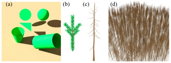
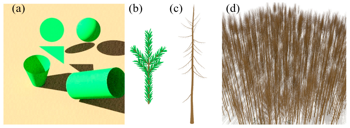
Figure 1.
Illustration of the RAMI-V actual scenario HET15_JBS_WIN. (a) Basic objects; (b) pine shoot; (c) trunk and branches of a tree; (d) the whole scene.
Table 1.
Structural and optical properties of ROMC validation scene HET01_DIS_UNI (HET01) and its derivatives.
A key feature of all RAMI-V scenes is the extensive use of the instancing technique, by organizing scene components into different hierarchical levels (hierarchies). This allows scenes containing numerous repetitive components to be represented as a set of instanced components combined with transformations (translation, rotation, and scaling). Instantiation greatly reduces the number of primitives, and hence the memory usage, compared with non-instanced scene descriptions. In RAMI-V, instancing is not only applied to generate trees across the entire scene but also canopy components within individual trees, such as broad leaves or pine shoots composed of multiple needle leaves.
To achieve a high level of detail in canopy representation, more complex curved objects (spheres, cylinders, and frusta) alongside simpler flat objects (disks and triangles) were introduced in actual scenarios. Combined by applying transformations to geometric primitives, realistic components and scenarios can be generated. Figure 1 schematically shows the basic objects (a), a pine shoot (b), the trunk and branches of a tree (c), and the whole scene of RAMI-V actual scenario HET15_JBS_WIN.
In MCRT models, the precise intersection point between a ray and a primitive needs to be determined. Then, the magnitude and directional distribution of scattered energy based on the surface properties at the intersection point are computed. Since RAMI-V actual scenarios utilize complex primitives to describe canopy components, ray-primitive intersection testing of the newly added curved objects within the MCRT model becomes a crucial issue affecting RT simulation accuracy. In addition, the instancing method to construct the scenarios needs corresponding acceleration of the bounding-box method to accommodate the scene description. In the next section, we introduce the newly implemented bounding-box method into the WPS and ray-primitive intersection methods for all the geometric objects used in the RAMI-V scenarios. Please refer to Section 2.3 for more details regarding the RAMI scenarios used for WPS evaluations.
2.2. The WPS RT Model
The WPS model is based on the forward MCRT approach by combining the photon spread method [16] and the weight reduction concept to simulate RT in architecturally realistic canopies [13]. Unlike LESS and DART-Lux based on open source renderers, which focus mainly on visual perception in the CG community, the WPS model was developed from scratch for simulations of RS hyperspectral signals. Since 2015, it has continuously evolved by incorporating new functionalities and by capitalizing on advances in CG to improve simulation efficiency. Its first major extension focused on fluorescence excitation to simulate the RT of solar-induced chlorophyll fluorescence (SIF) of 3D canopies [17]. Further extensions by modeling the radiative coupling between the atmosphere and land surface with the same MCRT technique made it possible for the non-fluorescent and SIF radiance received by sensors to be simulated by WPS at levels from the top of the canopy to the top of the atmosphere in a coherent manner [5]. Regarding the method used to represent plant canopies in WPS, two modes of scene representation can be differentiated. In one mode, the elements of the plant canopy, e.g., leaves, stems, stalks, branches, and background, are all explicitly represented by a number of geometric primitives (e.g., triangles and disks). Another mode abstracts the plants as volumetric primitives composed of a turbid medium. Since RAMI provides an explicit description of all scenarios, the explicit mode of the WPS model was adopted, using version 3.0, and hence a registered name of WPS3 was adopted for participation in RAMI-V.
2.2.1. Adaptation of the Bounding-Box Method for RAMI-V Scenarios
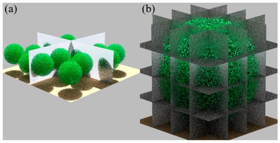
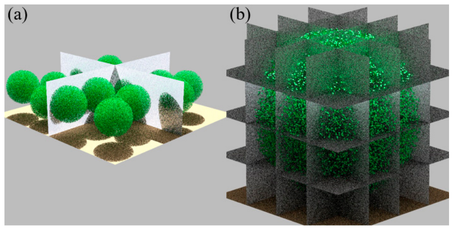
The original version, i.e., WPS3, loads all primitives’ coordinates before ray tracing, where each primitive’s position is explicitly defined without any rotational or translational matrix information. This mode uses a single-layer axis-aligned bounding-box (AABB) grid that partitions the entire scene elements into uniform cubic cells aligned with coordinate axes (Figure 2a). Each geometric primitive is assigned to the corresponding bounding box in which it resides. This simple scheme can accelerate ray tracing, since if a ray misses the bounding box, it cannot hit the object inside, and therefore there is no need to perform extra ray–primitive intersection tests.
Figure 2.
Schematic of the bounding box structure used in WPS. (a) Upper-layer division of the entire scene; (b) lower-layer division of an instanced canopy.
Since memory consumption in WPS3 scales nearly linearly with the number of primitives, highly detailed representation of complex scenarios containing tens or hundreds of millions of primitives may require excessive computer memory and simulation time, even for high-performance computers. For example, the abstract scene HOM23_DIS_P1A (79,579 objects) requires 54.7 MB of memory, whereas the actual scene HET15_JBS_WIN contains 138,251,607 objects, with a memory consumption of ~92.8 GB for loading only the coordinates of geometric primitives, far beyond typical capacities of personal computers. As described above, the instantiation technique was extensively used in RAMI-V to represent canopy scenes containing large numbers of repetitive elements. Therefore, an extension of WPS3 capable of handling such large and repetitive scenes was necessary to participate in the RAMI-V exercise. Consequently, two new modes, WPS3INS and WPS3BVH, were developed.
WPS3INS refers to the version for scenarios with object instancing, characterized by storing coordinates of all primitives within a sample canopy, along with the position of the sample canopy and transformation matrices (rotation and translation) applied to the sample canopy to generate the entire scene. This mode adopts a two-layer AABB scheme (Figure 2). The upper layer bounds the entire scene (Figure 2a), determining and recording the boxes containing each transformed canopy. The lower layer contains all the primitives within an instanced canopy (Figure 2b).
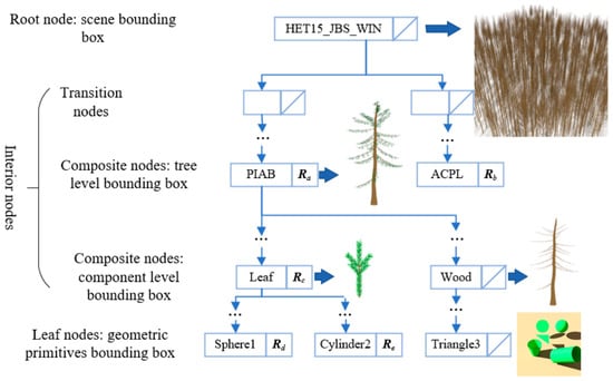
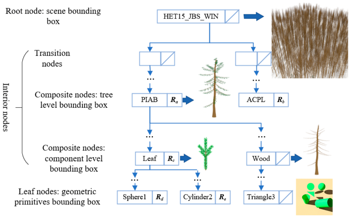
In some RAMI-V actual scenes, geometric primitives undergo scaling along coordinate axes followed by rotation and translation. For triangular facets, these transformations can be handled by directly updating vertex coordinates. However, for non-triangular surfaces, such as disks, cylinders, and frusta, repeated scaling and rotation cannot be precisely defined without explicitly recording the full transformation matrices. Retaining all transformation information for each primitive would dramatically increase memory usage. To address this issue, WPS3INS was further expanded with the Bounding Volume Hierarchy (BVH) structure [18], resulting in WPS3BVH. This mode ensures that each transformation is stored only once, thus avoiding redundant memory consumption. BVH consists of root, interior, and leaf nodes, with the root node representing the entire scene, leaf nodes corresponding to basic geometric primitives (disk, triangle, sphere, cylinder, and frustum, and their transformed shapes), and interior nodes storing bounding boxes and transformation matrices. Figure 3 shows a BVH tree structure for the scene HET15_JBS_WIN. The root node encloses the entire scene composed of all the trees. Interior nodes include transition nodes (without transformation matrices) and composite nodes (with transformation matrices). Composite nodes at the “tree” level contain bounding boxes for different tree types, e.g., virtual models PIAB (Norway spruce, Picea Abies) and ACPL (maple, Acer Platenoides), and their transformation matrices Ra and Rb. Composite nodes at the component level include bounding boxes for sub-elements such as leaves and wood and their transformations Rc. Leaf nodes contain the basic primitives, e.g., triangles, spheres, cylinders, and frusta, and their transformation matrices.
Figure 3.
Schematic of the bounding volume hierarchy tree structure used in WPS3BVH to construct the scene HET15_JBS_WIN. R with subscripts a, …, e, stands for the transformation matrix.
Theoretically, WPS3BVH can handle all scenarios of RAMI-V, WPS3INS is capable of handling most scenarios, excluding those with scaled non-triangular primitives, and WPS3 is suitable only for low-complexity cases (fewer than ~20 million primitives, ~16 GB RAM). In practice, the mode selection also depends on trade-offs among scene complexity, computer resources, and simulation efficiency. WPS3 was used for explicitly defined scenarios with low complexity, mainly the abstract scenarios. For actual scenarios composed of more than 20 million primitives (e.g., HET16_SRF_UND) with object instancing but without scaling transformations, WPS3INS was preferred over WPS3BVH, because WPS3BVH’s advantage in memory saving is marginal for such relatively low levels of hierarchies. For scenes with scaling transformations of non-triangular geometries (e.g., HET15_JBS_WIN), only WPS3BVH is applicable. Accordingly, the suitable WPS modes were adopted for the selected RAMI-V actual scenarios (Section 2.3.2).
2.2.2. Ray–Primitive Intersection
To adapt to RAMI-V actual scene definitions, we extended WPS’s capability to handle ray–primitive intersection for three new primitives and their transformed forms, i.e., spheres, cylinders, and frusta, besides the original two primitives, i.e., disks and triangles. The process of finding out where a ray hits an object is known as the ray–object intersection calculation. This is a fundamental process in the MCRT approach and usually takes most of the simulation time. This section describes the definition of primitives and the ray–object intersection calculation used in WPS.
To intersect rays with transformed objects, the following procedure in standard ray tracing [19] were adopted: (1) we intersected the inverse transformed ray with the untransformed object; (2) we calculated the normal to the untransformed object at the hit point; (3) we used the hit point on the untransformed object to compute where the original ray hits the transformed object; and (4) we used the normal to the untransformed object to compute the normal to the transformed object.
Since the problem of ray and transformed object intersection can always be converted into ray intersection with an untransformed object, below we present the methods to intersect the ray with all primitives without transformations. The object we ray trace is defined by an implicit surface equation with the form f (x, y, z) = 0, where f is some function of x, y, and z. We can also express the implicit surface using set notation as {(x, y, z): f (x, y, z) = 0}. A ray is an infinite straight line defined by an origin Po and direction d, , and t is the ray parameter and measures the distance along the ray from the origin. To intersect a ray with an implicit surface, we need to find the t that satisfies both the implicit surface equation and the ray equation, i.e., f (Po + td) = 0, where t is the only unknown. By substituting the smallest positive t into the ray equation, we obtain the coordinates of the nearest hit point.
Flat Objects: Disk and Triangle
An arbitrary disk is defined by its center C, normal n, and radius r. The center and normal define a plane in which the disk resides. The ray–disk intersection calculation starts with the ray–plane intersection and then checks if the hit point is located within distance r of the center.
A plane is specified by a point A that lies on the plane and a normal n to the plane. If the ray intersects the plane at P, then the following equation holds:
By solving Equation (1), a positive value of t can be obtained: t = (A − Po) · n/(d · n). Then, by comparing the distance between C and P and r, we can check whether the ray intersects the disk.
In a similar manner, to intersect a ray with a triangle, we first find where it hits the plane and then test if the hit point is within the triangle. Triangles are one of the most commonly used objects in CG. Efficient algorithms have been developed for ray–triangle intersection. The classical Möller and Trumbore [20] algorithm was adopted in WPS using barycentric coordinates. Please refer to the original article for details.
Curved Objects: Sphere, Cylinder and Frustum of a Cone
Spheres are the simplest type of curved surface and are a good starting point for ray intersection analysis for other curved objects in RAMI-V. The surface of a sphere is the set of points at distance r from a given point C (xc, yc, zc), {P: |P − C| = r}. If a ray intersects the sphere at point P = (x, y, z) on the surface of the sphere, the implicit equation is therefore
By substituting the parametric representation of the ray into the implicit sphere equation, we have
Note that all elements of this equation except for t are known values. By solving Equation (3) for the smaller positive root t, the nearest hit point on the sphere is obtained.
A circular cylinder centered around the z-axis with radius r and a finite extent in the z-direction is defined by {(x, y, z): x2 + y2 = r2 and z ∈ [0, h]}. Similar to the sphere case, the ray–cylinder intersection formula can be found by substituting the ray equation into the cylinder’s implicit equation, resulting in an equation like Equation (3) without z coordinates. The intersection algorithm of a ray with the two bases of a cylinder is the same as that for ray–disk intersection.
A frustum (of a cone) differs from a cylinder in that the radius of the former changes with height. Suppose the center of the frustum’s bottom disk is located at the origin of the Cartesian coordinates, with the radii of the bottom and top disks being r1 and r2 (r1 > r2), respectively. The radius rz at z between 0 and the perpendicular height h of the frustum is equal to r1 − (r1 − r2)z/h. Then, the set notation of a frustum can be expressed as {(x, y, z): x2 + y2 = rz2, rz = r1 − (r1 − r2)z/h, and z ∈ [0, h]}. The rest of the ray–frustum intersection algorithm is similar to that between a ray and a cylinder.
2.3. Model Evaluation and Intercomparison
Previously, we have shown favorable evaluation results for the WPS model via the ROMC platform [5,13], intercomparisons with the SCOPE model [13] and the coupled MODTRAN and SCOPE models [5], in situ hyperspectral measurements at ground level [13,17], and through unmanned aerial vehicles [5] and airplanes [21]. It is still necessary to evaluate WPS for the new extensions of bounding-box structures and the ray–primitive intersection test with dedicated evaluation designs. Regarding the ray–primitive intersection test, the procedure is straightforward and can be evaluated separately. Please refer to the Supplementary Data for the design of the ray–primitive intersection test (Figures S1–S3). This section mainly introduces experimental designs for evaluating the new extensions with RAMI abstract and actual scenarios.
2.3.1. Scenarios in ROMC
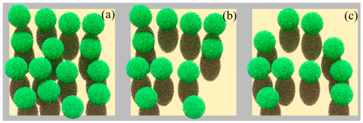
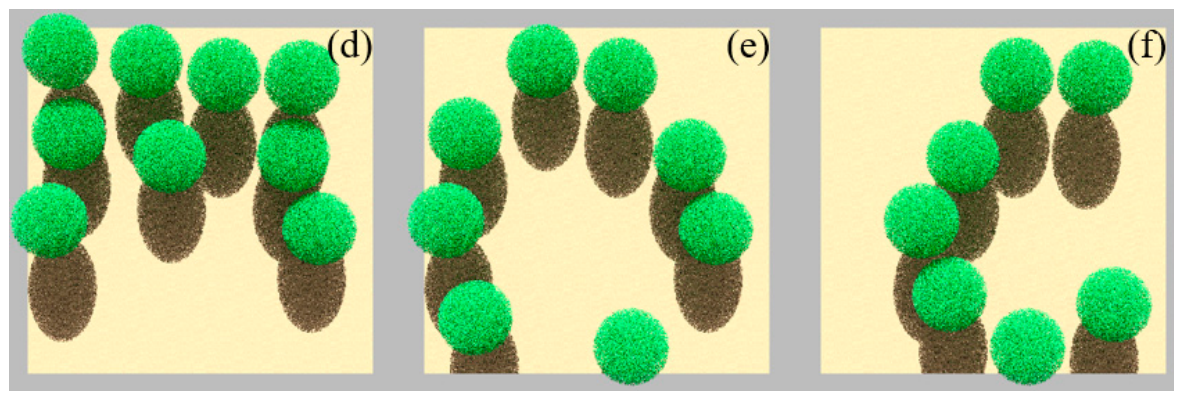
ROMC allows owners, users, and developers of RT models to unambiguously assess the performance of RT models in the forward mode. Two types of test canopy scenarios suggested by the ROMC organizers [9] are available from the ROMC website. One type is the horizontally homogeneous canopy “HOM11_DIS_ERE” and its derivatives. Another one is the heterogeneous 3D canopy scene “HET01_DIS_UNI” in a 100 m × 100 m section. The heterogeneous scene “HET01_DIS_UNI” and its derivatives, which are more relevant than the horizontally homogeneous scene, are chosen here to evaluate the WPS model with simulations of BRF in the principal plane (PP) or orthogonal plane (OP).
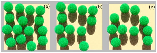
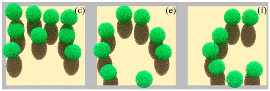
The scene HET01_DIS_UNI (denoted as HET01 for the sake of brevity) was generated with the simple instancing technique. A simple spherical envelope containing 49,999 randomly distributed finite size disk-shaped leaves represents a sample plant crown. HET01 includes 15 non-overlapping spherical envelopes, located over and only partially covering a horizontal plane standing for the underlying soil surface. Each disk-shaped scatterer is characterized by the specified radiative properties (reflectance and transmittance) in the red and NIR bands with a bi-Lambertian scattering law, and the orientation of the normals to the scatterers follows a uniform distribution function. The radiative properties of the underlying soil are also characterized by a Lambertian scattering law. By progressively removing some spherical envelopes, derivatives of HET01, i.e., HET11, HET21, HET31, HET41, and HET51, were generated in ROMC. Figure 4 illustrates top-view representations of the ROMC validation scenes.
Figure 4.
Top-view representations of the ROMC validation scene HET01_DIS_UNI (a) and its derivatives HET11 (b), HET21 (c), HET31 (d), HET41 (e), and HET51 (f).
There are two modes in ROMC to evaluate the quality of the test model [9]: (1) “debug mode”, which allows one to repeatedly compare the output of a RT model to the “surrogate truth” of one or more experiments; and (2) “validate mode”, which enables the once-only testing of the RT model against a randomly selected set of test cases that are similar but not quite equivalent to those from RAMI. Users of ROMC are encouraged to utilize ROMC results obtained in validate mode for publication purposes. Therefore, evaluations of the three modes via ROMC, WPS3, WPS3INS, and WPS3BVH, were carried out under validate mode, but they could not be performed on the same set of test cases. Table 1 provides the structural and spectral information of the canopy scenes. ROMC evaluation results were sent to the users in graphs. In the graphs, the “surrogate truth” dataset is denoted as “ROMCREF”.
2.3.2. Actual Scenes in RAMI-V
A set of MCRT models could agree within 2% uncertainty thresholds and could issue benchmark reference datasets for four actual RAMI-V scenarios, i.e., the birch stand in summer (HET09_JBS_SUM) and winter (HET15_JBS_WIN), and the structured canopy models consisting of the citrus orchard (HET14_WCO_UND) and the short-rotation poplar forest (HET16_SRF_UND) [8]. Two actual scenarios were selected here (see the reasons below) for evaluating different modes of WPS for BRF simulations at two characteristic bands: red (681.25 nm, RAMI-V band index: O10) and near infra-red (NIR, 753.75 nm, O12). Since the LESS model contributes to the benchmark datasets of RAMI-V actual scenarios [8], its simulated BRFs are presented for comparison.
The Short-Rotation Poplar Forest (HET16_SRF_UND)
Two crops in RAMI-V were provided with structured arrangement (planted in rows) of the trees, i.e., HET16_SRF_UND and HET14_WCO_UND. The poplar forest HET16_SRF_UND was constructed with object instancing at both tree and leaf levels, including triangles, hemispheres, cylinders, and frusta, with various transformations except for scaling. Therefore, all three versions of WPS can be applied. HET16_SRF_UND contains more primitive types and is structurally more complex than HET14_WCO_UND. Therefore, HET16_SRF_UND was selected to comprehensively evaluate three WPS modes. The scene is composed of broadleaf trees with a scene LAI of 3.219. Each leaf is described as 9 connected triangles. The trunk and branch are represented as hemispheres, cylinders, and frusta with their total area index of 0.588 (by analogy of LAI definition in coniferous canopies: one-half of the total surface area per unit of ground area).
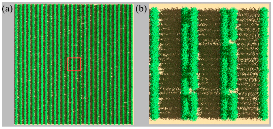
This scenario represents a step towards more realistic vegetation than the abstract scenario HET01_DIS_UNI in ROMC and is a good candidate to check the consistency among the three versions of WPS. Moreover, HET16_SRF_UND is one of four actual scenarios based on which WPS3INS could agree closely with other MCRT models (within 2% uncertainty), contributing to the benchmark for most of the virtual RS measurements. The full HET16_SRF_UND has dimensions of 99.8 m × 100.9 m × 3.4 m (Figure 5a) with 146,665,202 primitives, requiring ~98 GB RAM without the instancing technique. To accommodate WPS3 without instancing, the center part of the scene with both a width and length of 11 m was cropped as the structural input for all three modes of WPS (Figure 5b). However, when comparing with the LESS model, the whole scenario was employed for WPS3BVH and LESS.
Figure 5.
Top view of the whole HET16_SRF_UND scene with cropped region (red box) (a); zoomed-in top view of the cropped region (b).
The Birch Stand in Winter (HET15_JBS_WIN)
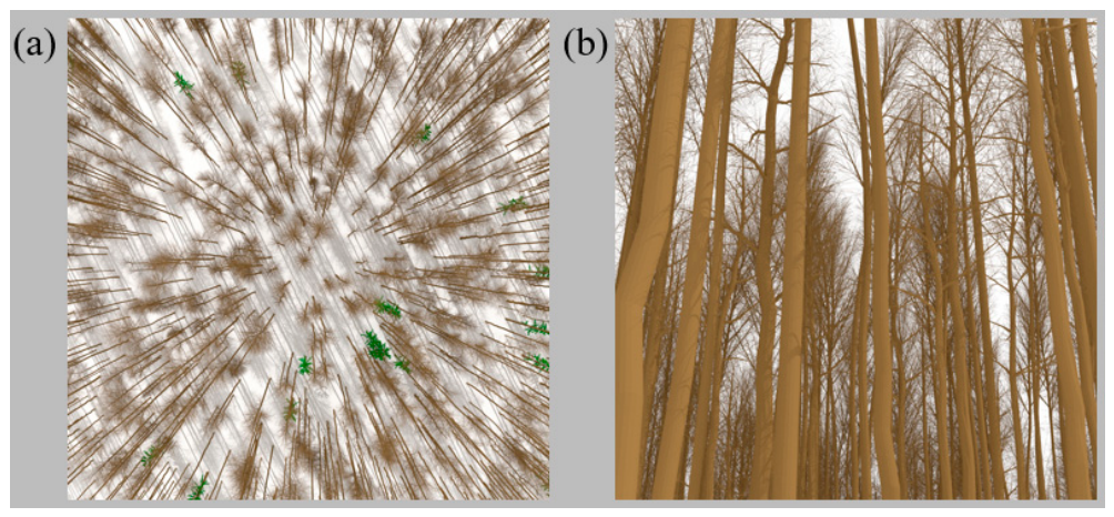
HET15_JBS_WIN and HET09_JBS_SUM represent the same birch forest scene in different seasons (winter and summer), with identical tree numbers and species. These are another two actual scenarios upon which WPS agrees closely with the benchmark reference datasets for most of the virtual measurements [8]. The winter scene HET15_JBS_WIN features higher background reflectance at O10 and O12 than the summer scene. The birch forest scene is composed of 1029 individual trees, with 990 being of broadleaf species, including maple, birch, alder, linden, poplar, and ash, and 39 being of coniferous species, specifically Norway spruce. Only the Norway spruce trees contain needle-shaped leaves (abstracted by ellipsoids), with an LAI of 0.0346. The trunks and branches of all trees are represented as triangles, with their total area index being 3.208. HET15_JBS_WIN includes triangles, ellipsoids, and cylinders, with all kinds of transformations including scaling, which means only WPS3BVH can be applied. HET15_JBS_WIN has a hierarchy level of 3, one level higher than HET16_SRF_UND. The leaf-on HET09_JBS_SUM contains more twigs (abstracted by hemispheres and cylinders) in broadleaf trees, which were ultimately simplified as triangles in LESS (see Section 4). However, no such simplifications for twigs were applied in WPS. So, to minimize the impact of scene description differences, HET15_JBS_WIN (whole scenario) was selected here to further evaluate WPS3BVH by comparing it with LESS. Figure 6 shows rendered images of the canopy scene.
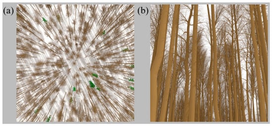
Figure 6.
Rendering of overview (a) and zoomed-in view (b) of the HET15_JBS_WIN scene.
The short-rotation poplar forest (HET16_SRF_UND) is a regularly planted, row-structured broadleaf canopy in which each leaf is described by nine connected triangles, so that the same small leaf element recurs a very large number of times: a scene in which object instancing is extremely effective. The birch stand in winter (HET15_JBS_WIN) is the same birch forest as the summer scene, with the same 1029 trees, observed in its leafless state, meaning that the trunks and branches described by triangles dominate the optical signal.
Two kinds of evaluation are used in this paper and should not be confused. (i) Validation is the comparison of WPS against an independent reference that is not produced by any of the models being tested: this is the ROMC surrogate truth, which is provided by ROMC and against which the accuracy of the three WPS modes is assessed (Section 3.1). (ii) Consistency checking is the comparison between WPS and another independently developed model over scenarios for which no absolute reference exists, i.e., the RAMI-V actual scenarios (Section 3.2). Agreement here shows that two independent implementations of the same physics, using different ray-tracing engines, do not diverge beyond a stated threshold. It constrains the magnitude of the implementation-level error but cannot establish absolute accuracy. MCRT estimates are stochastic because photons are randomly traced through the scene. The target radiation quantity is estimated by the sample mean of photon contributions. As in the Monte Carlo error analysis of WPS [5], the absolute error at a given confidence level is obtained from the standard deviation of the sample mean. The relative simulation error is calculated as the ratio of this absolute error and the estimated radiation quantity. All BRF simulations used 5 × 10⁵ photons. This photon number kept the relative Monte Carlo error below 1% at the 99.7% confidence level for the reported results.
3. Results
Evaluation results of the ray–primitive intersection test in the Supplementary Data show that ray–primitive intersection with spheres, cylinders, and frusta was correctly implemented (Figures S4–S6). Below, more comprehensive evaluations for the new extensions in WPS with RAMI abstract and actual scenarios are presented.
3.1. ROMC
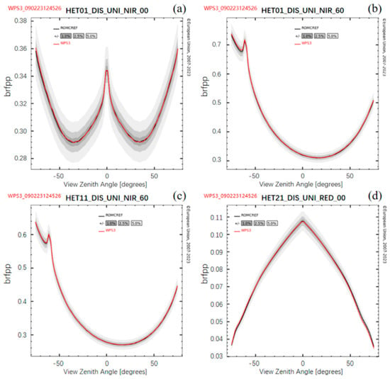
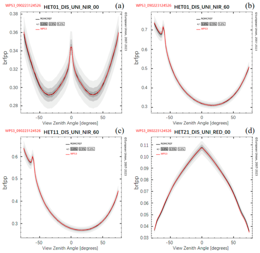
The BRFs simulated by three WPS modes (WPS3, WPS3INS, and WPS3BVH) over the ROMC validation scenes were benchmarked against the reference values provided by ROMC. Figure 7 shows comparisons of red and NIR BRF distributions in the principal plane (brfpp) and the orthogonal plane (brfop) simulated by WPS3 for HET01 (a and b), HET11 (c) and HET21 (d) with the “surrogate truth” solutions (noted as “ROMCREF”) under different sun zenith angles (SZAs). Three gray-colored envelopes corresponding to ±1%, ±2.5%, and ±5% of the BRF of the ROMCREF surround the reference solution. We can clearly see that all BRFs simulated by WPS3 are within ±1% of the “surrogate truth” solution.
Figure 7.
Comparison results of total BRFs simulated by WPS3 with the “surrogate truth” solutions (denoted as “ROMCREF”) in the principal planes. (a) BRF in NIR band for HET01 (SZA = 0°); (b) BRF in NIR band for HET01 (SZA = 60°); (c) BRF in NIR band for HET11 (SZA = 60°); (d) BRF in red band for HET21 (SZA = 0°).
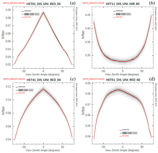
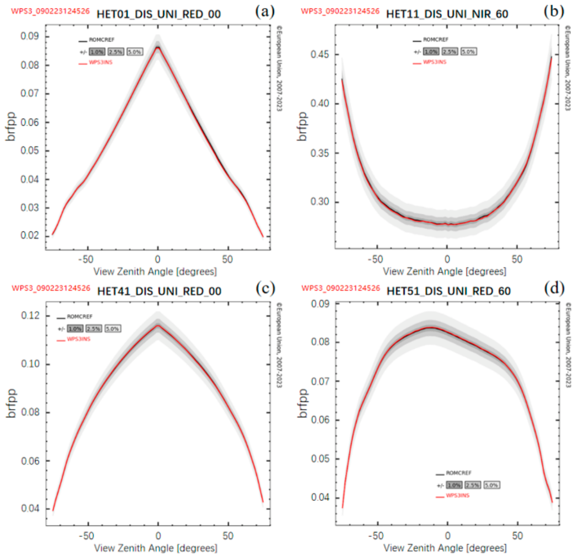
The scenes randomly assigned to WPS3INS are HET01 (Figure 8a), HET11 (Figure 8b), HET41 (Figure 8c), and HET51 (Figure 8d) for BRF simulations in the orthogonal planes. Figure 8 shows comparisons of BRF distributions in the red and NIR bands under different SZAs. Similarly, all BRFs simulated by WPS3INS are within ±1% of the “surrogate truth” solution.
Figure 8.
Comparison results of total BRFs simulated by WPS3INS with the “surrogate truth” solutions (noted as “ROMCREF”) in the orthogonal planes. (a) BRF in red band for HET01 (SZA = 0°); (b) BRF in NIR band for HET11 (SZA = 60°); (c) BRF in red band for HET41 (SZA = 0°); (d) BRF in red band for HET51 (SZA = 60°).
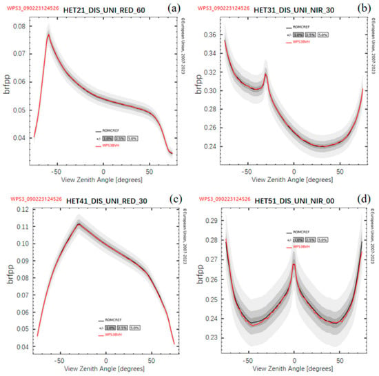
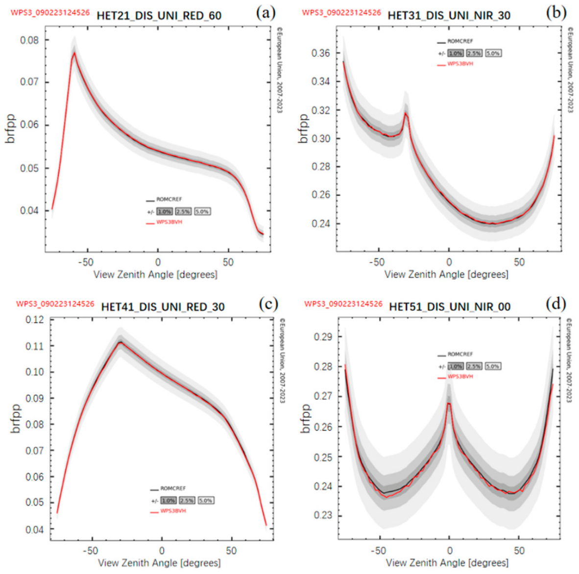
Figure 9 shows comparisons of BRF simulations by WPS3BVH in the red and NIR bands for HET21 (a), HET31 (b), HET41 (c), and HET51 (d), under different SZAs. Although BRF distributions by WPS3BVH in NIR for HET51 (Figure 9d) have relatively higher fluctuations, mainly due to slower convergence with the same amount of photons for the most sparse canopy and also small variations in BRF values, they are still within ±1% of the “surrogate truth” solution, as for other scenes.
Figure 9.
Comparison results of total BRFs simulated by WPS3BVH with the “surrogate truth” solutions (noted as “ROMCREF”) in the principal planes. (a) BRF in red band for HET21 (SZA = 60°); (b) BRF in NIR band for HET31 (SZA = 30°); (c) BRF in red band for HET41 (SZA = 30°); (d) BRF in NIR band for HET51 (SZA = 0°).
These comparison results show the generally very good agreement between ROMCREF and all three WPS modes, and among themselves. The abstract scene HET01 and its derivatives used the instancing technique of translation and rotation, but without scaling. Although their structures are relatively simple, the close agreements indicate that the new extension of the bounding-box method (two-layer AABB and BVH) and ray–object intersections with disks and triangles were correctly implemented in the three WPS modes.
3.2. Actual Scenarios of RAMI-V
3.2.1. The Short-Rotation Poplar Forest (HET16_SRF_UND)
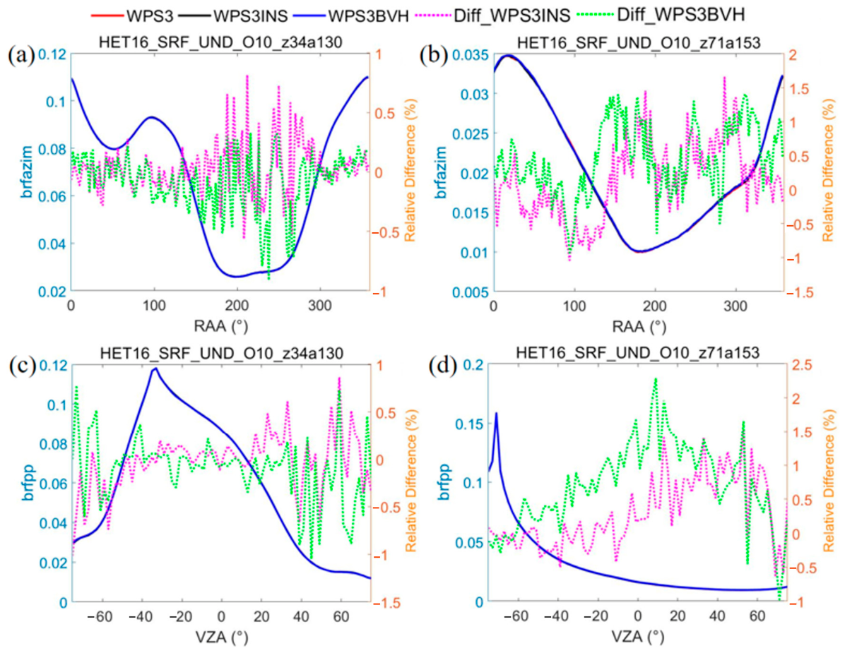
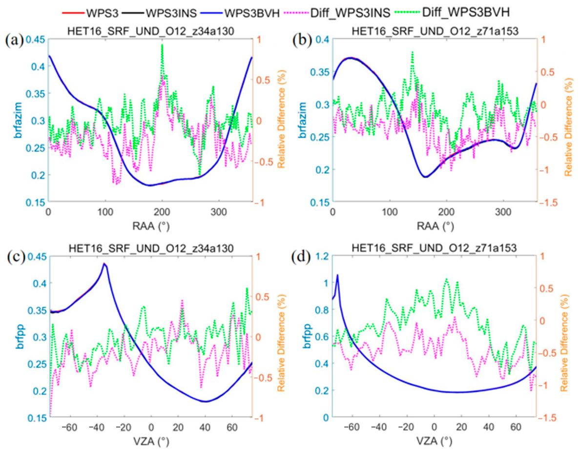
By referring to RAMI-V virtual measurement setups, BRFs were simulated in the PP (indicated as brfpp) and OP (brfop) with a resolution of 2° over the range of VZA from −75° (backward direction) to 75° (forward direction). BRFs were also provided in the azimuth ring (with a resolution of 2°) at a constant VZA of 37° (brfazim). Sun zenith and azimuth angles were set according to the average sun positions when Sentinel-3 OLCI overpasses the experimental site in Zerbolo, Italy, to generate HET16_SRF_UND in January–February and July, i.e., (71°, 153°) and (34°, 130°). Here, comparison results in PP and azimuth ring are presented. Statistical results in more viewing planes and comparison results with LESS are provided in Section 3.2.3. Choosing WPS3 simulations as a reference, the relative differences of three WPS modes were calculated as follows: Diff_WPS3INS = (BRFWPS3INS − BRFWPS3)/BRFWPS3 × 100%, Diff_WPS3BVH = (BRFWPS3BVH − BRFWPS3)/BRFWPS3 × 100%.
Figure 10 shows BRFs in the azimuth ring (a and b) and PP (c and d) at the red band (O10) simulated by the three WPS modes. The simulated BRF curves by the three modes are so close that they cannot be differentiated. As shown, the relative differences between WPS3 and both WPS3INS and WPS3BVH are all within ±2%.
Figure 10.
Simulated BRFs for the cropped HET16_SRF_UND scene in the red band using WPS3, WPS3INS, and WPS3BVH. (a) Azimuth ring (SZA = 34°, SAA = 130°), RAA (relative azimuth angle) = SAA − VAA; (b) azimuth ring (SZA = 71°, SAA = 153°); (c) principal plane (SZA = 34°, SAA = 130°); (d) principal plane (SZA = 71°, SAA = 153°).
For the NIR band (O12), the agreements of BRFs simulated by the three WPS modes are even closer than for the red band. As shown in Figure 11, the relative differences between WPS3 and both WPS3INS and WPS3BVH mostly remain within ±1%.
Figure 11.
Simulated BRFs for the cropped HET16_SRF_UND scene in the NIR band using WPS3, WPS3INS, and WPS3BVH. (a) Azimuth ring (SZA = 34°, SAA = 130°), RAA (relative azimuth angle) = SAA − VAA; (b) azimuth ring (SZA = 71°, SAA = 153°); (c) principal plane (SZA = 34°, SAA = 130°); (d) principal plane (SZA = 71°, SAA = 153°).
These inter-comparison results show good consistency among WPS3, WPS3INS, and WPS3BVH for more complex actual scenarios containing multiple primitive types (triangles, spheres, cylinders, and frusta) with translation and rotation transformations.
3.2.2. The Birch Stand in Winter (HET15_JBS_WIN)
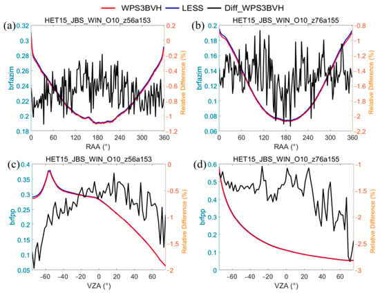
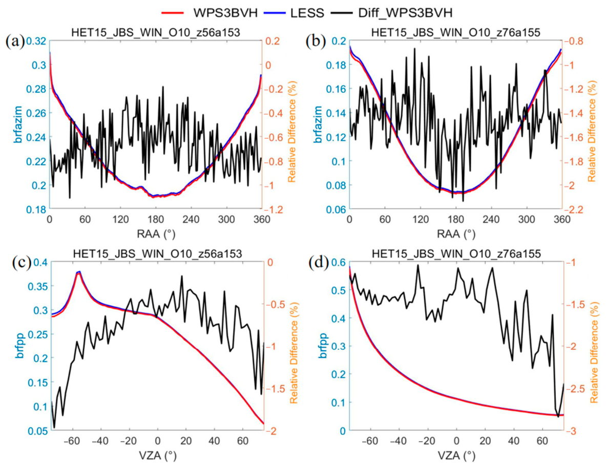
Only BRFs simulated by WPS3BVH were presented for comparison with LESS because HET15_JBS_WIN includes all kinds of transformations, including scaling, for primitives. It should be noted that LESS only allows triangular objects as inputs. So, ellipsoids and cylinders in the scene were simplified as two hexagonal pyramids and hexagonal prisms, respectively, and finally as triangles, based on surface-area-unchanged principle [15]. However, the impact of the simplifications should be small as the spruce trees contain needle-shaped leaves (abstracted by ellipsoids) with an LAI of 0.0346, much smaller than the total area index of trees’ trunks and branches (3.208). Figure 12 shows that BRFs in the red band simulated by WPS3BVH agree closely with those simulated by LESS. The relative differences between them, Diff_WPS3BVH = (BRFWPS3BVH − BRFLESS)/BRFLESS × 100%, are low, between −3% and 0, although the BRFs simulated by WPS3BVH are always lower than those simulated by LESS. The different RT simulation methods adopted by the two models may introduce this bias, which requires further investigation.
Figure 12.
Comparisons of simulated BRFs by WPS3BVH and LESS for HET15_JBS_WIN in the red band. (a) Azimuth ring (SZA = 56°, SAA = 153°), RAA (relative azimuth angle) = SAA − VAA; (b): azimuth ring (SZA = 76°, SAA = 155°); (c) principal plane (SZA = 56°, SAA = 153°); (d) principal plane (SZA = 76°, SAA = 155°).
The generally close accordance between WPS3BVH and LESS for simulating BRFs is consistent with the results indicating that the four MCRT models (DART, LESS, Raytran, and WPS) have good agreement for HET15_JBS_WIN, contributing to this credible reference group.
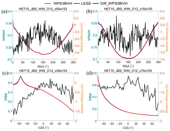
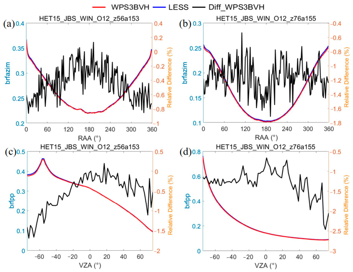
Comparisons in NIR (Figure 13) are similar to those in the red band, because trunks and branches dominate in the scene and their spectral properties in the red and NIR bands do not have as large differences as those for green leaves or needles. The relative differences between WPS3BVH and LESS are slightly lower, within (−2.5%, 0.2%), than those in the red band.
Figure 13.
Comparisons of simulated BRFs by WPS3BVH and LESS for HET15_JBS_WIN in the NIR band. (a) Azimuth ring (SZA = 56°, SAA = 153°), RAA (relative azimuth angle) = SAA − VAA; (b) azimuth ring (SZA = 76°, SAA = 155°); (c) principal plane (SZA = 56°, SAA = 153°); (d) principal plane (SZA = 76°, SAA = 155°).
3.2.3. Statistical Results Between WPS and LESS
To more comprehensively assess agreements between WPS and LESS for the actual scenarios, statistical metrics, R2 and Relative Root Mean Square Error (RRMSE), were computed between the WPS and LESS outputs for the red (O10) and NIR (O12) bands for the selected scenes (HET16_SRF_UND and HET15_JBS_WIN). Since the three WPS modes show very close agreement and their relative differences are within ±2% for HET16_SRF_UND and only WPS3BVH can be used for both scenarios, BRF simulations between WPS3BVH and LESS in the azimuth ring, PP, and OP were applied to calculate the statistical results (Table 2).
Table 2.
Statistical results of correlation between WPS3BVH and the LESS model for selected RAMI-V actual scenarios.
For HET16_SRF_UND and HET15_JBS_WIN, the agreements between the two models’ simulations are quite good, with a lowest R2 of 0.999 and highest RRMSE of ~1.553%. This high agreement is noteworthy because WPS, including its new extensions, was developed independently of LESS, which is based on a well-established rendering software Mitsuba [22]. Two independent implementations that share no code and rely on different ray-tracing engines would be expected to diverge substantially if either contained a systematic error of comparable size. The agreement therefore constrains the implementation error of WPS3BVH, but it does not by itself demonstrate physical accuracy; that evidence is provided by the ROMC validation in Section 3.1, where an external reference solution is available.
4. Discussion
The three modes of WPS differ in the adopted bounding-box methods. Their accuracy in simulating RT in canopies is comparable, as shown for the ROMC HET01_DIS_UNI and the cropped HET16_SRF_UND. Their differences in simulating RT come mainly from noise due to the random nature of MCRT per se. However, they differ a lot in runtime RAM usage and simulation efficiency. For the two scenarios, the computational costs for the three modes were compared (Table 3) based on a Windows-based personal computer with a CPU Intel core @2.10 GHz and RAM of 16 GB.
Table 3.
Computational costs of the three WPS modes for the BRF simulations of two RAMI scenarios.
Regarding runtime RAM usage, it follows a clear pattern for the same scene: WPS3 >> WPS3INS > WPS3BVH. Instantiation greatly reduces memory use for repetitive elements. Therefore, WPS3INS and WPS3BVH use far less memory than WPS3. The advantage of WPS3BVH over WPS3INS in memory reduction becomes greater with higher scene hierarchy level (HET16_SRF_UND).
Runtime does not show a consistent pattern across scenes. For HET01_DIS_UNI, runtime increases in the sequence of WPS3INS, WPS3, and WPS3BVH. For HET16_SRF_UND, runtime is lowest for WPS3 and highest for WPS3BVH, with WPS3INS in-between. WPS3BVH took the most time for both scenes due to the extra computational burden. To handle the intersection of rays with different nodes and transformed primitives within nodes, multiple transformations have to be performed (cf. Section 2.2.1). This additional computation reduces ray tracing’s efficiency. It took less time for WPS3INS over HET01_DIS_UNI than WPS3. However, the opposite is true over HET16_SRF_UND. The structural features of the two scenarios determine this difference. HET01_DIS_UNI is composed of non-overlapping spherical envelopes, for which two-layer bounding boxes could speed up the determination of components intersected with a ray. However, the envelopes of the trees in HET16_SRF_UND overlap a lot, which means canopy components may lie in multiple bounding-boxes, hence increasing intersection tests due to the two-layer box structure in WPS3INS.
Overall, WPS3BVH demonstrates the best memory saving performance but the lowest efficiency. WPS3INS exhibits moderate memory usage, with efficiency being dependent on canopy structure. Therefore, when participating in the RAMI-V exercise for actual scenarios, WPS3INS was preferred if it could be used (HET14_WCO_UND and HET16_SRF_UND). WPS3 consumes the most memory yet maintains relatively good runtime efficiency, meaning that it was mainly used for RAMI-V abstract scenarios.
It should be noted that the comparison of computational costs was performed based on single-thread execution mode because it isolates the algorithmic and data-structure differences among the three modes from parallel speed-up, which would otherwise dominate the comparison and obscure exactly the effect that the new scene representations produce. Nevertheless, MCRT is ideally suited to parallelization by dividing the tracing among multiple processors. In practice, simulation efficiency can be substantially improved via multi-thread and, in particular, GPU-based acceleration, which will be explored in our future extension.
Compared to implementing ray intersection tests with original primitives provided by RAMI actual scenarios, a different approach involves only using triangles for the canopy scene. This is possible, as adopted in LESS [15] and the DART model (https://dart.omp.eu/index.php#/doc, accessed on 24 September 2026), which tessellate all of the curved objects into triangles. This approach was not applied in WPS for the following reasons. First, the curved objects are not trivial to tessellate. Different tessellation methods can affect the BRF simulation results [15], therefore introducing uncertainties, particularly in the context of the ±1% accuracy target defined by RAMI. Second, their accurate representation may require such large numbers of triangles that RAM usage and simulation time increase significantly. Finally, a triangle-only approach does not take advantage of MCRT’s unmatched ability to ray trace exact mathematical representations of curved objects as compared to other RT methods, e.g., finite-element radiosity algorithms. As a result, the native RAMI scene descriptions are reserved as truthfully as possible, without any scene simplifications, which reduced uncertainties for the RT simulations over the 3D scenarios.
Since the objective of this paper is to introduce the extensions of the WPS model to natively support complex RAMI-V scene descriptions and its evaluation, the selection of experimental scenarios focused on well-controlled scene representations from simple abstract scenes with benchmark values (ROMC) to the more realistic RAMI-V actual scenarios, i.e., the short-rotation poplar forest (HET16_SRF_UND) and birch forest scene (HET15_JBS_WIN). For these scenarios, a credible reference group could be found to establish a reference dataset so that the extensions of the WPS model could be evaluated. In our follow-up study, we will explore the reasons for the high divergences in the RT simulations over the four RAMI-V actual scenarios among the participating MCRT models.
5. Conclusions
In this paper, we introduce new extensions of the WPS model and perform systematic evaluation of these new modes. By representing the 3D canopies with the instancing technique at hierarchical levels and handling ray–primitive intersection for different geometric primitives and their transformed forms, the RT simulations were made fully adaptable to the RAMI-V scenarios. These extensions ensured that the original RAMI-V scenarios are described as truthfully as possible, without any scene simplifications, which reduced uncertainties for the RT simulations over the 3D scenarios.
Evaluations through ROMC show that the accuracy of the new modes for 3D structure representation is within ±1% of the reference solution. For scenarios with triangular objects dominating in the scene, HET16_SRF_UND and HET15_JBS_WIN, the agreements of BRF simulations between WPS and LESS are quite good, with an R2 higher than 0.999 and an RRMSE lower than 1.554%, providing a consistency check between the two independent implementations. Based on the extended WPS model, we will explore the reasons for the high divergences in the RT simulations over some of the RAMI-V actual scenarios among the participating MCRT models in our follow-up study.
Supplementary Materials
The following supporting information can be downloaded at: https://www.mdpi.com/article/10.3390/rs18193331/s1.
Author Contributions
Conceptualization: F.Z.; Algorithm development and implementation: F.Z., X.L. and H.L.; Model evaluation: F.Z., J.L., H.L., J.Z., X.Z., D.X. and J.Q.; Writing of the original draft: F.Z.; Review and editing: F.Z., X.L., N.G. and C.L.; Funding acquisition: F.Z. All authors have read and agreed to the published version of the manuscript.
Funding
This work was funded by the Chinese Natural Science Foundation grant numbers 64742471515 and 41771382.
Data Availability Statement
All RAMI-V scenes description and files can be found on RAMI web site https://rami-benchmark.jrc.ec.europa.eu.
Acknowledgments
Feng Zhao would like to thank Zhilin Liu’s contribution on the early development of BVH module. We thank the reviewers’ comments to improve the paper.
Conflicts of Interest
Author Christian Lanconelli was employed by the company Uni Systems Italy. The remaining authors declare that the research was conducted in the absence of any commercial or financial relationships that could be construed as a potential conflict of interest.
References
- Kuusk, A. Canopy radiative transfer modeling. Compr. Remote Sens. 2018, 3, 9–22. [Google Scholar] [CrossRef] [Scilit]
- Goel, N. Models of vegetation canopy reflectance and their use in estimation of biophysical parameters from reflectance data. Remote Sens. Rev. 1988, 4, 1–212. [Google Scholar] [CrossRef] [Scilit]
- Disney, M.I.; Lewis, P.; North, P.R.J. Monte Carlo ray tracing in optical canopy reflectance modelling. Remote Sens. Rev. 2000, 18, 163–196. [Google Scholar] [CrossRef] [Scilit]
- Govaerts, Y.M.; Verstraete, M.M. Raytran: A Monte Carlo raytracing model to compute light scattering in three-dimensional heterogeneous media. IEEE Trans. Geosci. Remote Sens. 1998, 36, 493–505. [Google Scholar] [CrossRef] [Scilit]
- Zhao, F.; Li, Z.; Verhoef, W.; Fan, C.; Luan, H.; Yin, T.; Zhang, J.; Liu, Z.; Tong, C.; Bao, Y. Simulation of solar-induced chlorophyll fluorescence by modeling radiative coupling between vegetation and atmosphere with WPS. Remote Sens. Environ. 2022, 277, 113075. [Google Scholar] [CrossRef] [Scilit]
- Pinty, B.; Gobron, N.; Widlowski, J.L.; Gerstl, S.A.W.; Verstraete, M.M.; Antunes, M.; Bacour, C.; Gascon, F.; Gastellu, J.P.; Goel, N.; et al. Radiation transfer model intercomparison (RAMI) exercise. J. Geophys. Res. Atmos. 2001, 106, 11937–11956. [Google Scholar] [CrossRef] [Scilit]
- Pinty, B.; Widlowski, J.L.; Taberner, M.; Gobron, N.; Verstraete, M.M.; Disney, M.; Gascon, F.; Gastellu, J.P.; Jiang, L.; Kuusk, A.; et al. Radiation transfer model intercomparison (RAMI) exercise: Results from the second phase. J. Geophys. Res. Atmos. 2004, 109, D06210. [Google Scholar] [CrossRef] [Scilit]
- Lanconelli, C.; Gobron, N.; Robustelli, M.; Adams, J.S.; Calders, K.; Disney, M.; Gastellu-Etchegorry, J.-P.; Goodenough, A.; Govaerts, Y.; Hogan, R.J.; et al. The fifth phase of the Radiation Transfer Model Intercomparison Exercise (RAMI-V): Experiment description and results on actual canopy scenarios. J. Remote Sens. 2025, 5, 0663. [Google Scholar] [CrossRef] [Scilit]
- Widlowski, J.L.; Robustelli, M.; Disney, M.; Gastellu-Etchegorry, J.P.; Lavergne, T.; Lewis, P.; North, P.R.J.; Pinty, B.; Thompson, R.; Verstraete, M.M. The RAMI on-line model checker (ROMC): A web-based benchmarking facility for canopy reflectance models. Remote Sens. Environ. 2008, 112, 1144–1150. [Google Scholar] [CrossRef] [Scilit]
- Gastellu-Etchegorry, J.P.; Demarez, V.; Pinel, V.; Zagolski, F. Modeling radiative transfer in heterogeneous 3-D vegetation canopies. Remote Sens. Environ. 1996, 58, 131–156. [Google Scholar] [CrossRef] [Scilit]
- Wang, Y.; Kallel, A.; Yang, X.; Regaieg, O.; Lauret, N.; Guilleux, J.; Chavanon, E.; Gastellu-Etchegorry, J.P. DART-Lux: An unbiased and rapid Monte Carlo radiative transfer method for simulating remote sensing images. Remote Sens. Environ. 2022, 274, 112973. [Google Scholar] [CrossRef] [Scilit]
- Qi, J.; Xie, D.; Yin, T.; Yan, G.; Gastellu-Etchegorry, J.P.; Li, L.; Zhang, W.; Mu, X.; Norford, L.K. LESS: LargE-Scale remote sensing data and image simulation framework over heterogeneous 3D scenes. Remote Sens. Environ. 2019, 221, 695–706. [Google Scholar] [CrossRef] [Scilit]
- Zhao, F.; Li, Y.; Dai, X.; Verhoef, W.; Guo, Y.; Shang, H.; Huang, J. Simulated impact of sensor field of view and distance on field measurements of bidirectional reflectance factors for row crops. Remote Sens. Environ. 2015, 156, 129–142. [Google Scholar] [CrossRef] [Scilit]
- Widlowski, J.L.; Mio, C.; Disney, M.; Adams, J.; Andredakis, I.; Atzberger, C.; Brennan, J.; Busetto, L.; Chelle, M.; Ceccherini, G.; et al. The fourth phase of the radiative transfer model intercomparison (RAMI) exercise: Actual canopy scenarios and conformity testing. Remote Sens. Environ. 2015, 169, 418–437. [Google Scholar] [CrossRef] [Scilit]
- Zhou, K.; Xie, D.; Qi, J.; Zhang, Z.; Bo, X.; Yan, G.; Mu, X. Explicitly reconstructing RAMI-V scenes for accurate 3-dimensional radiative transfer simulation using the LESS model. J. Remote Sens. 2023, 3, 0033. [Google Scholar] [CrossRef] [Scilit]
- Thompson, R.L.; Goel, N.S. Two models for rapidly calculating bidirectional reflectance of complex vegetation scenes: Photon spread (PS) model and statistical photon spread (SPS) model. Remote Sens. Rev. 1998, 16, 157–207. [Google Scholar] [CrossRef] [Scilit]
- Zhao, F.; Dai, X.; Verhoef, W.; Guo, Y.; van der Tol, C.; Li, Y.; Huang, Y. FluorWPS: A Monte Carlo ray-tracing model to compute sun-induced chlorophyll fluorescence of three-dimensional canopy. Remote Sens. Environ. 2016, 187, 385–399. [Google Scholar] [CrossRef] [Scilit]
- Müller, G.; Fellner, D. Hybrid scene structuring with application to ray tracing. In Proceedings of the International Conference on Visual Computing (ICVC’99), Goa, India, 23–26 February 1999; pp. 19–26. [Google Scholar]
- Pharr, M.; Jakob, W.; Humphreys, G. Physically Based Rendering: From Theory to Implementation, 3rd ed.; Morgan Kaufmann: Waltham/Burlington, MA, USA, 2017. [Google Scholar] [CrossRef] [Scilit]
- Möller, T.; Trumbore, B. Fast, minimum storage ray-triangle intersection. J. Graph. Tools 1997, 2, 21–28. [Google Scholar] [CrossRef] [Scilit]
- Tong, C.; Bao, Y.; Zhao, F.; Fan, C.; Li, Z.; Huang, Q. Evaluation of the FluorWPS model and study of the parameter sensitivity for simulating solar-induced chlorophyll fluorescence. Remote Sens. 2021, 13, 1091. [Google Scholar] [CrossRef] [Scilit]
- Jakob, W. Mitsuba Physically Based Renderer. 2010. Available online: http://www.mitsuba-renderer.org (accessed on 24 September 2026).

Disclaimer/Publisher’s Note: The statements, opinions and data contained in all publications are solely those of the individual author(s) and contributor(s) and not of MDPI and/or the editor(s). MDPI and/or the editor(s) disclaim responsibility for any injury to people or property resulting from any ideas, methods, instructions or products referred to in the content. |
© 2026 by the authors. Licensee MDPI, Basel, Switzerland. This article is an open access article distributed under the terms and conditions of the Creative Commons Attribution (CC BY) license.