CoGLoR: Collaborative Global–Local Representation Learning for Remote Sensing Scene Classification

Highlights

What are the main findings?

• A collaborative global–local self-supervised framework, CoGLoR, is proposed for remote sensing scene classification by jointly integrating global contrastive learning, masked reconstruction, and Contrastive Patch-Level Attention Matching.
• C-PAM replaces fixed index-wise positives with a hard top-K, multi-positive feature neighborhood when augmented views are not spatially registered.

What are the implications of the main findings?

• The results indicate that explicitly coordinating global scene semantics and local structural details improves the quality and label efficiency of self-supervised remote sensing representations.
• CoGLoR provides an effective representation learning strategy for label-scarce remote sensing scene classification, where reliable annotations are limited or costly to obtain.

Abstract

Self-supervised learning provides an effective way to reduce the dependence on manual annotations in remote sensing scene classification. However, existing self-supervised methods often emphasize either global semantic invariance or local structural modeling, while the interaction between global scene context and local patch-level representations remains insufficiently explored. This limitation is important for remote sensing images, whose scene categories are usually determined by both holistic spatial layouts and fine-grained local objects. To address this issue, we propose CoGLoR, a collaborative global–local representation learning framework for self-supervised remote sensing scene classification. The proposed framework jointly integrates global contrastive learning, masked reconstruction, and Contrastive Patch-Level Attention Matching within a unified training pipeline. The contrastive branch learns scene-level semantic consistency across augmented views, while the reconstruction branch encourages the encoder to preserve local structural details by reconstructing masked patches. C-PAM replaces fixed spatial indices with a hard top-K, multi-positive feature neighborhood and contrasts the selected neighbors against batch-level candidates. The selected features are treated as learned neighbors rather than verified semantic correspondences. Experiments on AID, UCMerced Land Use, and NWPU-RESISC45 show that CoGLoR improves over representative contrastive learning, masked modeling, and hybrid self-supervised baselines under linear probing and low-label evaluation protocols. The matched ResNet-50 comparison supports the method-level evaluation; the retrieval figure illustrates cosine-ranking behavior; the ViT-S/16 experiment tests backbone portability; and the resource table quantifies pretraining overhead. Externally pretrained methods are included only as contextual references.

1. Introduction

Remote sensing scene classification is a fundamental task in Earth observation and supports a wide range of applications, including land-use monitoring, urban planning, environmental assessment, disaster response, and resource management [1]. A recent review further summarizes the development and application scope of deep learning methods for this task [2]. Remote sensing observations are also used in environmentally sensitive cold regions, for example, to evaluate ground-surface freeze–thaw dynamics and vegetation interactions on the Qinghai–Xizang Plateau [3]. Unlike natural-image classification, remote sensing scene classification faces several distinctive challenges, such as large viewpoint variations, substantial intra-class diversity, strong inter-class similarity, and the coexistence of multiple semantic objects within a single scene. For example, airport, port, industrial, and residential scenes are usually characterized not by a single dominant object, but by the spatial configuration of multiple local regions and the overall land-use layout. Therefore, effective remote sensing scene representations should capture both global semantic context and fine-grained local structures.

Deep learning methods, including convolutional neural networks and vision transformers, have significantly improved the performance of remote sensing scene classification. Discriminative CNNs learn scene representations from labeled samples [4]. Transformer-based architectures have also been explored for remote sensing image classification [5]. However, most high-performing models still rely on fully supervised training and require large-scale annotated datasets. In practical remote sensing applications, collecting reliable annotations is expensive and time-consuming, because image interpretation often requires expert knowledge. The limited availability of labeled samples therefore remains a major constraint for training robust and transferable scene-classification models. Similar demands for adaptable representations arise in site-specific monitoring scenarios; for example, time-series InSAR has been used to monitor surface deformation in Yakutsk, a city located in a continuous-permafrost region [6].

Self-supervised learning (SSL) provides a promising solution by learning visual representations from unlabeled data [7]. Among existing SSL paradigms, contrastive learning and masked image modeling (MIM) are two representative directions. SimCLR learns augmentation-invariant representations by contrasting different views of each image [8]. MoCo introduces a momentum encoder and a dynamic queue for contrastive learning [9]. DenseCL extends contrastive supervision to dense local features [10]. SimSiam shows that Siamese representation learning can also operate without explicit negative pairs [11]. In contrast, MIM-based methods learn representations by reconstructing masked image content. MAE reconstructs missing patches with an asymmetric encoder–decoder architecture [12]. BEiT predicts visual tokens for masked patches [13]. SimMIM demonstrates the effectiveness of a simple pixel-reconstruction objective [14].

Despite their effectiveness, both paradigms have limitations for remote sensing scene classification. Contrastive learning mainly operates on global image-level representations and may underutilize small but discriminative local regions, such as aircraft, ships, storage tanks, buildings, and roads. MIM improves local-detail modeling through reconstruction, but reconstruction alone does not necessarily lead to strong scene-level discrimination. Thus, contrastive learning and MIM provide complementary supervision: the former emphasizes global semantic invariance, while the latter preserves local structural information. A simple combination of these objectives, however, does not explicitly model the interaction between local patch features and global scene context.

Another important issue arises from spatial augmentations. Remote sensing SSL commonly uses random cropping, rotation, and scale transformation to improve robustness. Under these augmentations, patch features at the same spatial index in two views may no longer correspond to the same semantic region. Therefore, hard index-wise feature alignment can introduce noisy supervision and weaken the effectiveness of global–local collaboration. This problem is particularly relevant for remote sensing images, where important objects may appear at different positions or scales across augmented views.

To address these issues, we propose CoGLoR (Collaborative Global–Local Representation Learning), a self-supervised framework for remote sensing scene classification. CoGLoR integrates three complementary objectives in a unified architecture. First, a global contrastive branch learns scene-level semantic invariance from two augmented views. Second, a masked reconstruction branch feeds a masked view into the shared encoder and reconstructs missing patches to preserve local structural details. Third, we introduce a Contrastive Patch-Level Attention Matching (C-PAM) objective to establish correspondence between masked-view patch tokens and unmasked-view patch tokens. C-PAM does not introduce a learned attention layer or assume ground-truth semantic identity. Its specific contribution is a hard top-K, multi-positive feature-neighborhood rule that replaces fixed indices and uses batch-level contrastive candidates.

Extensive experiments are conducted on three widely used remote sensing scene classification benchmarks, including AID, UCMerced Land Use, and NWPU-RESISC45. The evaluation covers linear probing and low-label classification settings to assess the quality and label efficiency of the learned representations. Experimental results show that CoGLoR improves the performance of remote sensing scene classification compared with representative contrastive learning, masked modeling, and hybrid self-supervised baselines.

The main contributions of this work are summarized as follows:

• We propose CoGLoR, a collaborative self-supervised framework for remote sensing scene classification that jointly learns global semantic invariance and local structural details through contrastive learning and masked reconstruction. The framework contribution is positioned as integration rather than as the first global–local remote sensing SSL method.
• We introduce a Contrastive Patch-Level Attention Matching objective to replace hard spatial-index alignment. The novel element tested here is the hard top-K, multi-positive, batch-contrastive neighborhood rule and its reference-view and neighborhood-size choices.
• We conduct extensive experiments on AID, UCMerced Land Use, and NWPU-RESISC45, showing that the proposed method improves over representative self-supervised baselines under linear probing and low-label classification settings. Additional experiments examine same-backbone comparisons, qualitative matching behavior, backbone portability, and computational cost.

2. Related Work

2.1. Remote Sensing Scene Classification and Self-Supervised Learning

Remote sensing scene classification aims to assign semantic labels to aerial or satellite images according to their land-use or scene-level content. Compared with natural images, remote sensing images usually contain larger scale variations, arbitrary object orientations, complex backgrounds, and multiple semantic objects within the same scene. These characteristics make scene classification highly dependent on both the global spatial layout and local discriminative structures [1]. A recent meta-analysis provides a broader review of deep learning strategies for remote sensing image scene classification [2].

Supervised scene-classification models have progressively improved feature discrimination and local-structure modeling. A discriminative CNN framework combines deep representation learning with metric learning [4]. Multiple-instance densely connected ConvNet models scene-level information from local instances [15]. Local Semantic Enhanced ConvNet further strengthens the contribution of semantically meaningful regions [16]. The AGOS framework learns multigrain instance representations for aerial scene classification [17]. Transformer-based architectures have also been explored for remote sensing image classification [5]. In parallel, Million-AID expands the scale and diversity of aerial-image benchmark construction [18].

Despite this progress, supervised methods generally require sufficient labeled samples. In practice, collecting high-quality annotations for remote sensing images is costly and often requires domain expertise. Self-supervised learning provides an alternative solution by learning transferable representations from unlabeled data [7]. Zhao et al. combine multiple self-supervised tasks for remote sensing scene classification [19]. Berg et al. review the state of self-supervised scene classification in remote sensing and discuss open challenges [20]. Chen et al. investigate self-supervised learning with partially unlabeled remote sensing datasets [21]. Attention GANs provide an unsupervised route for learning aerial-scene features [22]. SCL-MLNet applies self-supervised contrastive learning to few-shot scene classification [23]. A general self-supervised framework has also been evaluated for remote sensing image classification [24]. Spectral–spatial self-supervised representation learning has been studied for unlabeled remote sensing imagery [25]. Seasonal Contrast uses uncurated remote sensing data for unsupervised pretraining [26]. SatMAE extends masked pretraining to temporal and multispectral satellite imagery [27].

However, designing effective SSL objectives for remote sensing remains challenging. Remote sensing scenes are not only characterized by global semantic categories, but also by fine-grained objects and spatial arrangements. Recent studies have further explored adaptive masked pretraining, multi-view contrastive learning, and foundation-model-based representation learning for remote sensing, reflecting the growing interest in label-efficient and transferable feature learning. Nevertheless, effectively coordinating scene-level invariance with fine-grained local structural information remains an important problem. Therefore, a suitable SSL framework should learn both scene-level semantic invariance and local structural information, which motivates the development of global–local collaborative pretraining strategies.

2.2. Contrastive Learning for Visual Representation

Contrastive learning is one of the most widely used paradigms in self-supervised visual representation learning. SimCLR learns representations by pulling together different augmented views of the same image and pushing apart views from different images [8]. MoCo maintains a queue of encoded samples to support contrastive learning with a large and consistent dictionary [9]. SimSiam further removes the need for negative samples by using prediction and stop-gradient mechanisms [11]. DenseCL extends contrastive learning from image-level representations to dense local features, showing that local correspondences can improve dense prediction and representation learning [10].

In remote sensing, contrastive learning has also been explored for scene classification and domain-specific representation learning. Spatially augmented momentum contrast improves unsupervised embedding for remotely sensed images [28]. Spatial–temporal invariant contrastive learning exploits domain-specific invariances for scene classification [29]. These methods are effective at learning global semantic invariance and improving robustness to image transformations.

Nevertheless, image-level contrastive learning may underutilize small but important local regions. This limitation is particularly relevant for remote sensing scene classification, where local objects such as aircraft, ships, roads, storage tanks, and buildings can be essential for distinguishing visually similar categories. Therefore, contrastive learning alone may produce representations that are globally consistent but insufficiently sensitive to local discriminative structures.

2.3. Masked Image Modeling and Local Structure Learning

Masked image modeling has become another important SSL paradigm. Inspired by masked language modeling, MAE learns representations by reconstructing missing image patches [12]. BEiT instead predicts discrete visual tokens for masked regions [13]. SimMIM shows that a lightweight reconstruction head can provide an effective masked-modeling objective [14]. Unlike contrastive learning, MIM does not mainly rely on instance discrimination. Instead, it encourages the encoder to capture local structure, texture, and contextual dependency through reconstruction.

For remote sensing images, masked modeling is naturally attractive because local structures and spatial patterns are important for scene understanding. SatMAE demonstrates masked pretraining for temporal and multispectral satellite imagery [27]. Related remote sensing SSL frameworks also preserve spatial information through reconstruction-oriented pretext tasks [24]. Spectral–spatial representation learning provides another route for exploiting unlabeled remote sensing imagery [25]. However, reconstruction alone may focus on low-level appearance recovery and does not necessarily guarantee strong scene-level discrimination. A model trained only to reconstruct missing patches may learn detailed local textures, but the resulting representation may still be suboptimal for category-level scene classification.

Therefore, contrastive learning and masked image modeling provide complementary supervision. The former emphasizes global semantic discrimination, while the latter improves local structural modeling. The key problem is how to combine them effectively rather than simply optimizing two independent pretext tasks.

2.4. Hybrid Self-Supervised Learning and Global–Local Alignment

Recent studies have attempted to combine contrastive learning and masked modeling to exploit their complementary strengths. iBOT performs self-distillation with an online tokenizer for masked image modeling [30]. Masked Siamese Networks introduce masking into Siamese representation learning [31]. CMAE combines contrastive learning and masked autoencoding to strengthen visual representation learning [32]. These methods demonstrate that combining discriminative and reconstructive objectives can improve self-supervised representation learning.

DenseCL and VICRegL already establish dense or local cross-view objectives [10,33]; SiameseIM and CMAE combine discriminative learning with masked prediction or reconstruction [32,34]; and CMID provides a closely related global–local remote sensing framework [35]. Scale-MAE, DINOv2, and recent remote sensing foundation-model work further show the importance of pretraining scale and architecture [36,37,38]. These studies preclude a broad novelty claim based only on combining global and local objectives.

However, directly transferring these ideas to remote sensing scene classification still leaves several issues. First, many hybrid SSL methods are developed mainly for natural images and may not explicitly consider the spatial composition and scale variation in remote sensing scenes. Second, some methods rely on token-level correspondence or teacher–student prediction, but the relationship between local remote sensing patches and scene-level context is not always explicitly modeled. Third, under strong augmentations such as random cropping, hard index-wise feature alignment may become unreliable because the same spatial index in two views may correspond to different semantic regions.

The proposed CoGLoR addresses these issues by introducing a collaborative global–local framework tailored for remote sensing scene representation learning. It integrates global contrastive learning, masked reconstruction, and Contrastive Patch-Level Attention Matching (C-PAM). Unlike hard spatial-index alignment, C-PAM selects top-K related patches from the corresponding unmasked view and formulates patch alignment as a contrastive objective. Relative to the closest families above, the defensible distinction is the particular hard top-K, multi-positive, batch-contrastive rule applied between a masked CNN feature map and an independently augmented reference view; the broader ideas of hybrid SSL and dense correspondence are prior concepts.

3. Materials and Methods

This section presents the proposed collaborative global–local self-supervised framework for remote sensing scene classification. The motivation is that remote sensing scenes are determined by both holistic spatial layouts and fine-grained local objects. While contrastive learning captures global semantic invariance, it may ignore local structures that are critical for distinguishing similar land-use categories. Masked image modeling improves local-detail preservation by reconstructing missing patches, but it provides limited scene-level discriminative supervision. In addition, direct spatial-index alignment between two augmented views is unreliable under random cropping, since the same patch index may correspond to different semantic regions.

To overcome these issues, the proposed framework integrates three complementary objectives. First, global contrastive loss is applied to two augmented views to learn scene-level semantic consistency. Second, masked reconstruction loss is computed by feeding a masked view into the shared encoder and reconstructing the missing patches, which strengthens local structural modeling. Third, Contrastive Patch-Level Attention Matching (C-PAM) loss is introduced to form feature-similarity neighborhoods between masked-view and unmasked-view patch tokens. Unlike hard index-wise alignment, C-PAM selects the top-K most similar patches from the corresponding unmasked view as feature-neighborhood positives and performs patch-level contrastive alignment against batch-level patch candidates. This formulation reduces noisy index-wise alignment caused by spatial mismatch and provides local feature-level supervision for remote sensing representation learning.

3.1. Overall Framework Architecture

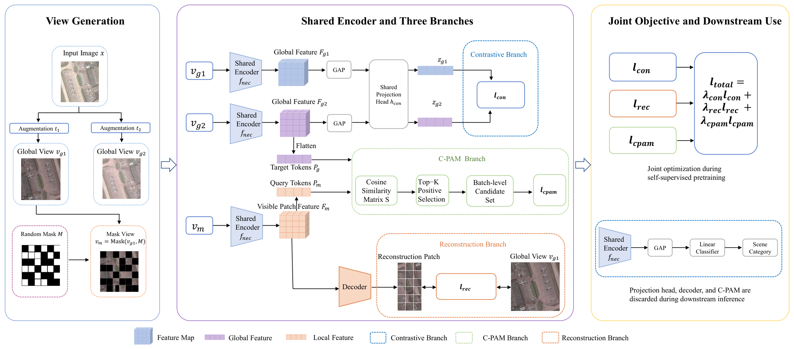
The overall architecture of the proposed framework is shown in Figure 1. Given an unlabeled remote sensing image $x\in \mathcal{D}$, two stochastic augmentation functions $t_1$ and $t_2$ are applied to generate two global views:

$$v_{g1}=t_1\left(x\right),v_{g2}=t_2\left(x\right).$$

(1)

The augmentations include random resized cropping, flipping, rotation, color jittering, grayscale transformation, and Gaussian blurring. To construct the masked branch, a random patch mask $\mathcal{M}$ is further applied to $v_{g1}$, producing a masked view $v_m$:

$$v_m=\mathrm{Mask}(v_{g1},\mathcal{M}).$$

(2)

Figure 1. Overall architecture of CoGLoR. Two independently augmented global views and one masked view pass through the same encoder in three forward operations. Global contrast, masked reconstruction, and C-PAM update the shared encoder during pretraining; only the encoder is retained for downstream evaluation.

The framework consists of a shared encoder $f_{\mathrm{enc}}$, a contrastive projection head $h_{\mathrm{con}}$, and a lightweight reconstruction decoder $f_{\mathrm{dec}}$. The two global views $v_{g1}$ and $v_{g2}$ are fed into the shared encoder to obtain spatial feature maps $F_{g1}$ and $F_{g2}$:

$$F_{g1}=f_{\mathrm{enc}}\left(v_{g1}\right),F_{g2}=f_{\mathrm{enc}}\left(v_{g2}\right).$$

(3)

Global average pooling followed by the projection head maps these features into the contrastive embedding space for scene-level contrastive learning.

The masked view $v_m$ is also passed through the same encoder:

$$F_m=f_{\mathrm{enc}}\left(v_m\right).$$

(4)

The reconstruction decoder takes $F_m$ as input and predicts the missing image content. The reconstruction loss is computed only over the masked patch positions. Meanwhile, the spatial feature maps $F_m$ and $F_{g2}$ are flattened into patch-token sequences:

$$P_m=\mathrm{Flatten}\left(F_m\right)\in {\mathbb{R}}^{N_m\times C},P_g=\mathrm{Flatten}\left(F_{g2}\right)\in {\mathbb{R}}^{N_g\times C},$$

(5)

where C is the feature dimension and $N_m$, $N_g$ denote the number of patch tokens.

The training objective contains three coupled components. The global contrastive branch learns scene-level semantic invariance from $v_{g1}$ and $v_{g2}$. The masked reconstruction branch encourages local structural modeling from $v_m$. The C-PAM branch performs contrastive patch-level feature matching between $P_m$ and $P_g$, which reduces unreliable index-wise alignment under random cropping and provides discriminative supervision for local representations. All components share the same encoder and are optimized jointly.

3.2. Global Contrastive Learning for Scene-Level Semantics

The global contrastive branch is used to learn scene-level representations that are invariant to common remote sensing transformations while remaining discriminative across different images. Given two augmented global views $v_{g1}$ and $v_{g2}$, the shared encoder extracts their spatial feature maps:

$$F_{g1}=f_{\mathrm{enc}}\left(v_{g1}\right),F_{g2}=f_{\mathrm{enc}}\left(v_{g2}\right).$$

(6)

Global descriptors are then obtained by global average pooling and mapped into a contrastive embedding space by the projection head:

$$z_{g1}=h_{\mathrm{con}}\left(\mathrm{GAP}\left(F_{g1}\right)\right),z_{g2}=h_{\mathrm{con}}\left(\mathrm{GAP}\left(F_{g2}\right)\right).$$

(7)

For each image in a mini-batch, the embeddings from its two augmented views form a positive pair, while embeddings from different images serve as negative samples. We adopt symmetric InfoNCE loss [39]:

$${\mathcal{L}}_{\mathrm{con}}=-{\displaystyle \frac{1}{2B}}{\displaystyle {\sum }_{i=1}^B}\left[\log {\displaystyle \frac{\exp (\mathrm{sim}(z_{g1}^i,z_{g2}^i)/{\tau }_{\mathrm{con}})}{{\sum }_{j=1}^B\exp (\mathrm{sim}(z_{g1}^i,z_{g2}^j)/{\tau }_{\mathrm{con}})}}+\log {\displaystyle \frac{\exp (\mathrm{sim}(z_{g2}^i,z_{g1}^i)/{\tau }_{\mathrm{con}})}{{\sum }_{j=1}^B\exp (\mathrm{sim}(z_{g2}^i,z_{g1}^j)/{\tau }_{\mathrm{con}})}}\right],$$

(8)

where B is the batch size, ${\tau }_{\mathrm{con}}$ is the temperature parameter, and

$$\mathrm{sim}(u,v)={\displaystyle \frac{u^{\top }v}{\parallel u\parallel \parallel v\parallel }}$$

(9)

denotes cosine similarity.

By pulling together the two views of the same image and contrasting them against other images, this branch encourages the encoder to capture robust global semantics, including land-use patterns, spatial layout, and scene-level context. These global representations provide the semantic basis for the subsequent local reconstruction and patch-level alignment branches.

3.3. Masked Reconstruction for Local Structural Modeling

The masked reconstruction branch is introduced to enhance local structural modeling. While global contrastive learning captures scene-level semantics, it may overlook fine-grained objects and spatial patterns that are important for remote sensing scene classification. To preserve such local information, one augmented view $v_{g1}$ is divided into a regular patch grid, and a random subset of patches $\mathcal{M}$ is masked to generate the masked view $v_m$:

$$v_m=\mathrm{Mask}(v_{g1},\mathcal{M}).$$

(10)

The masked view is then fed into the shared encoder:

$$F_m=f_{\mathrm{enc}}\left(v_m\right),$$

(11)

and the reconstruction decoder predicts the missing image content:

$$\widehat{x}=f_{\mathrm{dec}}\left(F_m\right).$$

(12)

The reconstruction loss is computed only over the masked patch positions:

$${\mathcal{L}}_{\mathrm{rec}}={\displaystyle \frac{1}{\left|\mathcal{M}\right|}}\sum _{i\in \mathcal{M}}{∥{\widehat{x}}_i-x_i∥}_2^2,$$

(13)

where $x_i$ denotes the original patch from $v_{g1}$ and ${\widehat{x}}_i$ denotes the corresponding reconstructed patch.

By reconstructing missing regions from partially observed inputs, this branch encourages the encoder to retain local texture, boundary, object shape, and spatial arrangement information. These local cues complement the global semantic invariance learned by the contrastive branch and provide a more detailed representation for remote sensing scene classification.

3.4. Contrastive Patch-Level Attention Matching for Feature Alignment

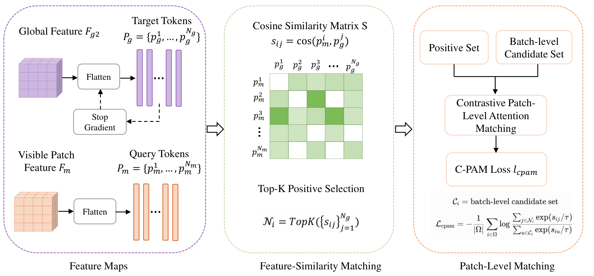
Directly aligning patch features at the same spatial index is unreliable under strong spatial augmentations. In particular, random cropping may cause two features with the same index from different views to correspond to different semantic regions. To avoid such noisy supervision, we introduce a Contrastive Patch-Level Attention Matching (C-PAM) module, which forms feature-similarity neighborhoods between masked-view patch tokens and unmasked-view patch tokens. The detailed C-PAM procedure is illustrated in Figure 2.

Figure 2. C-PAM for one masked-view query. Cosine similarity ranks detached reference tokens from $F_{g2}$; the top-K tokens form the multi-positive numerator, while eligible batch-level tokens form the contrastive denominator.

Let

$$P_m=\{p_m^1,p_m^2,\dots ,p_m^{N_m}\}\in {\mathbb{R}}^{N_m\times C}$$

(14)

denote the patch-token sequence extracted from the masked view $v_m$, and let

$$P_g=\{p_g^1,p_g^2,\dots ,p_g^{N_g}\}\in {\mathbb{R}}^{N_g\times C}$$

(15)

denote the patch-token sequence extracted from the unmasked global view $v_{g2}$. For each source token $p_m^i$, we first compute its cosine similarity with all target tokens from the corresponding unmasked view:

$$s_{ij}={\displaystyle \frac{{\left(p_m^i\right)}^{\top }{p}_g^j}{\parallel p_m^i\parallel \parallel p_g^j\parallel }},j=1,\dots ,N_g.$$

(16)

The top-K most similar target tokens are selected as the positive feature neighbors of $p_m^i$:

$${\mathcal{N}}_i=\mathrm{TopK}\left({\left\{s_{ij}\right\}}_{j=1}^{N_g}\right).$$

(17)

Instead of directly regressing $p_m^i$ to an already similar soft target, we formulate the alignment as a patch-level contrastive objective. For each source token $p_m^i$, the positive set is formed by its top-K matched tokens from the same image, while all target tokens in the mini-batch are used as contrastive candidates. The C-PAM loss is defined as:

$${\mathcal{L}}_{\mathrm{cpam}}=-{\displaystyle \frac{1}{|\Omega |}}\sum _{i\in \Omega }\log {\displaystyle \frac{{\sum }_{j\in {\mathcal{N}}_i}\exp (\mathrm{sim}(p_m^i,p_g^j)/{\tau }_{\mathrm{pam}})}{{\sum }_{b=1}^B{\sum }_{k=1}^{N_g}\exp (\mathrm{sim}(p_m^i,p_{g,b}^k)/{\tau }_{\mathrm{pam}})}},$$

(18)

where $\Omega$ denotes the set of source tokens involved in alignment, B is the mini-batch size, $N_g$ is the number of target tokens in each unmasked view, and ${\tau }_{\mathrm{pam}}$ is the temperature parameter for patch-level contrastive matching. The C-PAM loss updates the masked-view source-token pathway against target-token references from the unmasked view. As described below, the target patch features are detached during training to stabilize the alignment process.

The reference features are taken from $F_{g2}$ because $F_m$ is constructed from a masked version of $v_{g1}$; using the independently augmented $v_{g2}$ prevents the default rule from reducing to same-crop content recovery. Ablations compare $F_{g1}$, $F_{g2}$, and their combination. The selected top-K tokens are treated as feature-neighborhood positives, not as verified semantic correspondences.

This formulation differs from hard index-wise alignment in two aspects. First, the positive targets are determined by feature similarity rather than spatial index, which reduces mismatches caused by random cropping. Second, the contrastive denominator introduces batch-level patch candidates, making the alignment objective discriminative rather than a simple feature regression. As a result, C-PAM encourages masked-view local tokens to identify high-similarity reference neighbors from the unmasked view under batch-level contrastive normalization.

3.5. Overall Objective Function

The proposed framework is optimized by jointly combining global contrastive learning, masked reconstruction, and Contrastive Patch-Level Attention Matching. The total objective is defined as:

$${\mathcal{L}}_{\mathrm{total}}={\lambda }_{\mathrm{con}}{\mathcal{L}}_{\mathrm{con}}+{\lambda }_{\mathrm{rec}}{\mathcal{L}}_{\mathrm{rec}}+{\lambda }_{\mathrm{cpam}}{\mathcal{L}}_{\mathrm{cpam}},$$

(19)

where ${\lambda }_{\mathrm{con}}$, ${\lambda }_{\mathrm{rec}}$, and ${\lambda }_{\mathrm{cpam}}$ control the contributions of the three losses.

Each objective provides a different supervisory signal. The contrastive loss encourages global scene-level discrimination across augmented views. The reconstruction loss preserves local structural information by recovering masked patches from partially observed inputs. The C-PAM loss further provides patch-level feature-neighborhood alignment between the masked view and the unmasked view under a contrastive formulation. By optimizing these objectives jointly, the encoder learns representations that are globally discriminative, locally structure-aware, and robust to spatial transformations.

3.6. Training and Evaluation Protocol

Before self-supervised pretraining, each dataset is first divided into class-stratified training and test partitions. Only images from the training partition are used for self-supervised pretraining, with their class labels discarded. The held-out test partition is not used during pretraining or downstream classifier training and is reserved exclusively for final evaluation.

During self-supervised pretraining, the shared encoder, projection head, and reconstruction decoder are jointly optimized using the objective in Equation (19). In the C-PAM branch, the target patch features from the unmasked reference view are detached from the computation graph to stabilize the alignment process.

After pretraining, only the encoder $f_{\mathrm{enc}}$ is retained for downstream evaluation, while the projection head and reconstruction decoder are discarded. For linear probing, the pretrained encoder is frozen, and a linear classifier is trained on the global pooled features using the labeled training partition. For low-label evaluation, the same frozen-encoder protocol is adopted, but the linear classifier is trained using class-stratified subsets containing 1%, 5%, and 10% of the training partition. The same held-out test partition is used for final evaluation in all settings.

These protocols evaluate the linear separability and label efficiency of the frozen self-supervised representations while maintaining a strict separation between pretraining/training data and the held-out test data.

4. Results

This section evaluates the proposed CoGLoR framework on remote sensing scene classification benchmarks. We first describe the experimental datasets, evaluation protocols, implementation details, and comparison methods. Then, we report quantitative results under linear probing and low-label classification settings to assess the transferability and data efficiency of the learned representations. Finally, ablation studies and qualitative visualizations are provided to analyze the contribution of each component and the effect of the proposed Contrastive Patch-Level Attention Matching module.

4.1. Experimental Setup

4.1.1. Datasets

We evaluate the proposed method on three widely used remote sensing scene classification benchmarks: AID [40], NWPU-RESISC45 [1], and UC Merced Land Use (UCM) [41]. These datasets differ in scale, number of categories, spatial resolution, and intra-class variability, providing a comprehensive evaluation of representation quality and generalization ability.

AID is a challenging aerial scene classification dataset with diverse imaging conditions and substantial intra-class variation. It contains multiple land-use and scene categories, covering complex urban, rural, and natural environments. Due to its large visual diversity and strong inter-class similarity, AID is used to evaluate whether the proposed method can learn discriminative representations that capture both global scene layouts and local structural cues.

NWPU-RESISC45 is a large-scale remote sensing scene classification benchmark with a broader category set and higher visual diversity. It includes various scene types collected from different geographic regions and imaging conditions. Compared with AID and UCM, NWPU-RESISC45 provides a more challenging testbed for evaluating the scalability and robustness of self-supervised representations.

UC Merced Land Use is a compact but widely adopted benchmark for remote sensing scene classification. It is used for cross-study comparison and for assessing representation transfer under limited-data conditions. Its relatively small scale also makes it suitable for evaluating the data efficiency of self-supervised pretraining.

Using these three datasets allows us to examine the proposed method from complementary perspectives: AID for medium-scale scene representation learning, NWPU-RESISC45 for large-scale generalization, and UCM for compact-benchmark transfer and low-label evaluation.

4.1.2. Evaluation Protocols

Before self-supervised pretraining, each dataset is first divided into training and test partitions using a class-stratified split. Only images from the training partition are used for self-supervised pretraining, with their class labels discarded. The test partition is completely excluded from self-supervised pretraining and classifier training and is used only for final evaluation.

Linear probing. After self-supervised pretraining, the encoder $f_{\mathrm{enc}}$ is frozen, and only a linear classifier is trained on top of the global pooled feature using the labeled training partition. The same held-out test partition is then used to evaluate the linear separability of the learned representations.

Low-label classification. To assess label efficiency, class-stratified subsets containing 1%, 5%, and 10% of the training partition are sampled to train the linear classifier. The sampling is performed independently within each class. For a given labeling ratio, the number of selected samples from each class is determined as $\max (1,\lfloor N_{c}r\rfloor )$, where $N_c$ denotes the number of samples of class c in the training partition and r is the labeling ratio. This rule ensures that at least one labeled sample is retained for each class. Accordingly, the total numbers of labeled training samples for the 1%, 5%, and 10% settings are 35, 239, and 493 for AID; 135, 765, and 1575 for NWPU-RESISC45; and 21, 42, and 105 for UCM, respectively.

The pretrained encoder remains frozen. The test partition remains unchanged and is used only for final evaluation.

For quantitative evaluation, we report overall accuracy. All experiments are repeated with multiple random seeds, and the mean and standard deviation are reported.

4.1.3. Implementation Details

CoGLoR is implemented in PyTorch (version 2.2.2) using ResNet-50 as the encoder backbone [42]. The projection head consists of a two-layer multilayer perceptron, and the reconstruction decoder is implemented as a lightweight upsampling decoder. Input images are resized to $224\times 224$ during both self-supervised pretraining and downstream evaluation.

For self-supervised pretraining, two augmented global views are generated for each input image. The augmentation pipeline includes random resized cropping with a scale range of $[0.4,1.0]$ and an aspect-ratio range of $[3/4,4/3]$, random horizontal flipping with probability $0.5$, random rotation within $[-{90}^{\circ },{90}^{\circ }]$, color jittering with brightness, contrast, saturation, and hue factors of $0.4$, $0.4$, $0.4$, and $0.05$, respectively, random grayscale transformation with probability $0.2$, and Gaussian blurring with probability $0.5$ and $\sigma \in [0.1,2.0]$. A random patch mask is further applied to one augmented view to construct the masked input for the reconstruction branch. The default patch size is set to $16\times 16$, and the masking ratio is set to 0.75 unless otherwise stated.

The model is pretrained for 100 epochs with a batch size of 128 using the AdamW optimizer. The initial learning rate is set to $3\times {10}^{-4}$ and the weight decay is set to 0.05. No learning-rate warm-up is used, and a cosine learning-rate schedule is adopted throughout pretraining.

The total loss follows Equation (19), where ${\lambda }_{\mathrm{con}}$, ${\lambda }_{\mathrm{rec}}$, and ${\lambda }_{\mathrm{cpam}}$ are used to balance the contrastive, reconstruction, and C-PAM losses, respectively. In our default setting, ${\lambda }_{\mathrm{con}}=1.0$, ${\lambda }_{\mathrm{rec}}=1.0$, and ${\lambda }_{\mathrm{cpam}}=0.5$. The temperature parameter is set to 0.10. The top-K value in C-PAM is set to 5 by default.

For downstream evaluation, the pretrained encoder is frozen, and a linear classifier is trained on top of the global pooled feature using the labeled training partition. For low-label evaluation, class-stratified subsets containing 1%, 5%, and 10% of the training partition are used to train the linear classifier. The held-out test partition remains unchanged and is used only for final evaluation. All baseline results reported in this study are obtained from our local reproductions. All comparison methods use the same input resolution, class-stratified train–test split, low-label sampling procedure, and downstream evaluation protocol. For the locally reproduced methods, the same pretraining budget of 100 epochs and a batch size of 128 is used to ensure a comparable training setting.

All reported experiments are repeated over five independent runs using random seeds $\{42,43,44,45,46\}$, and the mean and standard deviation are reported.

The downstream experiments reported in this study use a frozen encoder. They should therefore be interpreted as linear probing and low-label linear evaluation, not as end-to-end fine-tuning.

4.2. Comparison with Self-Supervised Methods

We compare CoGLoR with representative self-supervised methods.

All baseline results reported in Table 1, Table 2, Table 3 and Table 4 are obtained from our local reproductions; no numerical results are taken directly from previous publications.

Table 1. Controlled in-domain comparison, cross-backbone validation, and additional locally reproduced baselines. Values are OA (%, mean ± standard deviation over repeated runs).

Method	Backbone	AID	NWPU	UCM
Matched in-domain comparison
SimCLR [8]	ResNet-50	95.53 ± 0.14	93.84 ± 0.18	97.42 ± 0.22
DenseCL [10]	ResNet-50	96.02 ± 0.32	94.65 ± 0.26	97.89 ± 0.20
CoGLoR	ResNet-50	97.14 ± 0.16	96.13 ± 0.17	98.48 ± 0.16
Cross-backbone validation
iBOT [30]	ViT-S/16	95.86 ± 0.14	94.46 ± 0.16	97.81 ± 0.18
CoGLoR	ViT-S/16	96.90 ± 0.21	96.57 ± 0.35	98.22 ± 0.27
Additional reproduced baselines
CMID [35]	ResNet-50	96.75 ± 0.30	95.46 ± 0.28	98.09 ± 0.19
Scale-MAE [36]	ViT-L/16	96.87 ± 0.23	95.82 ± 0.39	98.13 ± 0.21

Table 2. Comparison with representative self-supervised methods on the AID dataset. Linear probing is evaluated under the 50% training split, and low-label results are reported using class-stratified subsets containing 1%, 5%, and 10% of the training partition. Best performance is shown in bold.

Method	Linear Acc. (%)	Low-Label Acc. (%)
		1%	5%	10%
SimCLR [8]	95.53 ± 0.14	83.85 ± 0.48	91.04 ± 0.36	93.12 ± 0.22
MoCo [9]	95.28 ± 0.16	83.41 ± 0.42	90.72 ± 0.32	92.85 ± 0.26
MAE [12]	95.71 ± 0.12	84.09 ± 0.30	91.24 ± 0.26	93.34 ± 0.17
iBOT [30]	95.86 ± 0.14	84.35 ± 0.37	91.57 ± 0.25	93.68 ± 0.18
Masked Siamese Networks [31]	95.63 ± 0.20	84.18 ± 0.31	91.35 ± 0.22	93.56 ± 0.21
CMAE [32]	96.12 ± 0.15	84.46 ± 0.34	91.73 ± 0.36	93.82 ± 0.17
CoGLoR (Ours)	97.14 ± 0.16	85.27 ± 0.28	92.78 ± 0.24	94.74 ± 0.18

Table 3. Comparison with representative self-supervised methods on the NWPU-RESISC45 dataset. Linear probing is evaluated under the 50% training split, and low-label results are reported using class-stratified subsets containing 1%, 5%, and 10% of the training partition. Best performance is shown in bold.

Method	Linear Acc. (%)	Low-Label Acc. (%)
		1%	5%	10%
SimCLR [8]	93.84 ± 0.18	83.36 ± 0.51	88.47 ± 0.39	89.73 ± 0.31
MoCo [9]	93.52 ± 0.21	82.94 ± 0.48	88.11 ± 0.42	89.41 ± 0.34
MAE [12]	94.18 ± 0.17	84.05 ± 0.44	89.06 ± 0.36	90.32 ± 0.28
iBOT [30]	94.46 ± 0.16	84.48 ± 0.41	89.52 ± 0.33	90.76 ± 0.26
Masked Siamese Networks [31]	94.31 ± 0.19	84.26 ± 0.46	89.37 ± 0.35	90.63 ± 0.29
CMAE [32]	94.83 ± 0.15	84.92 ± 0.39	90.14 ± 0.31	91.25 ± 0.24
CoGLoR (Ours)	96.13 ± 0.17	86.27 ± 0.36	91.67 ± 0.29	92.87 ± 0.22

Table 4. Comparison with representative self-supervised methods on the UC Merced Land Use dataset. Linear probing is evaluated under the 50% training split, and low-label results are reported using class-stratified subsets containing 1%, 5%, and 10% of the training partition. At least one labeled sample is retained per class when required. Best performance is shown in bold.

Method	Linear Acc. (%)	Low-Label Acc. (%)
		1%	5%	10%
SimCLR [8]	97.42 ± 0.22	78.36 ± 0.86	88.74 ± 0.58	93.21 ± 0.41
MoCo [9]	97.18 ± 0.25	77.95 ± 0.91	88.31 ± 0.62	92.86 ± 0.45
MAE [12]	97.63 ± 0.20	79.12 ± 0.78	89.26 ± 0.54	93.58 ± 0.38
iBOT [30]	97.81 ± 0.18	79.65 ± 0.73	89.71 ± 0.50	93.94 ± 0.34
Masked Siamese Networks [31]	97.69 ± 0.21	79.43 ± 0.76	89.52 ± 0.53	93.82 ± 0.36
CMAE [32]	98.04 ± 0.17	80.16 ± 0.69	90.18 ± 0.47	94.36 ± 0.31
CoGLoR (Ours)	98.48 ± 0.16	81.45 ± 0.65	91.36 ± 0.42	95.12 ± 0.29

SimCLR, MoCo, and CoGLoR use ResNet-50 encoders, while MAE, iBOT, Masked Siamese Networks, and CMAE use ViT-based encoders.

All compared methods use the same $224\times 224$ input resolution, class-stratified train–test split, low-label sampling procedure, and downstream evaluation protocol.

Table 2, Table 3 and Table 4 summarize the results under linear probing and low-label classification settings. In the linear probing protocol, the pretrained encoder is frozen, and a linear classifier is trained using the labeled training partition. In the low-label setting, the same frozen-encoder protocol is adopted using class-stratified subsets containing 1%, 5%, and 10% of the training partition. The held-out test partition is kept fixed and is used only for final evaluation.

Because Table 2, Table 3 and Table 4 include methods with different backbone architectures, these results are interpreted as cross-backbone comparisons rather than strictly controlled method-level comparisons. The primary controlled comparison is the matched ResNet-50 track in Table 1, which uses the same experimental protocol described above.

Against DenseCL, the strongest matched ResNet-50 baseline, CoGLoR improves OA by 1.12, 1.48, and 0.59 percentage points on AID, NWPU-RESISC45, and UCM, respectively. The ViT-S/16 comparison provides complementary cross-backbone evaluation, while the matched ResNet-50 comparison serves as the primary controlled method-level comparison.

Across the three datasets, CoGLoR consistently outperforms the compared SSL baselines. The following tables report how the gains change with dataset complexity and label availability.

• Quantitative analysis.

CMAE is the best-performing competing method in every reported setting. CoGLoR improves upon CMAE consistently. On AID, CoGLoR increases linear-probing accuracy from 96.12% to 97.14%, a gain of 1.02 percentage points. Under the 1%, 5%, and 10% low-label settings, the corresponding gains are 0.81, 1.05, and 0.92 percentage points, respectively. Adding C-PAM yields further improvements over the parallel combination of global contrastive learning and masked reconstruction.

On NWPU-RESISC45, which contains a broader range of scene categories and greater visual diversity, CoGLoR outperforms CMAE by 1.30 percentage points under linear probing and by 1.35, 1.53, and 1.62 percentage points when training subsets containing 1%, 5%, and 10% of the training partition are used. The gains are observed across all label ratios. In this setting, visually similar categories may require local objects and structural arrangements for classification.

On UCM, CoGLoR increases linear-probing accuracy from 98.04% to 98.48%. Under the 1%, 5%, and 10% low-label settings, CoGLoR improves upon CMAE by 1.29, 1.18, and 0.76 percentage points, respectively. The improvements are also observed under limited supervision.

When averaged across the three datasets, CoGLoR improves upon the best-performing competing baseline by 0.92 percentage points under linear probing and by 1.15, 1.25, and 1.10 percentage points under the 1%, 5%, and 10% low-label settings. The gains are larger on the more diverse NWPU-RESISC45 benchmark and under restricted-label protocols. Additional classification metrics under the controlled linear- probing protocol are reported in Table 5.

Table 5. Additional classification metrics under the controlled linear-probing protocol. Results are reported as mean ± standard deviation over repeated runs.

Dataset	Method	OA (%)	Macro-F1 (%)	Kappa (%)
AID	DenseCL [10]	96.02 ± 0.32	95.74 ± 0.37	95.80 ± 0.34
AID	CoGLoR	97.14 ± 0.16	96.93 ± 0.21	96.98 ± 0.17
NWPU	DenseCL [10]	94.65 ± 0.26	94.35 ± 0.31	94.41 ± 0.28
NWPU	CoGLoR	96.13 ± 0.17	95.91 ± 0.23	95.94 ± 0.19
UCM	DenseCL [10]	97.89 ± 0.20	97.72 ± 0.25	97.76 ± 0.22
UCM	CoGLoR	98.48 ± 0.16	98.34 ± 0.21	98.38 ± 0.18

Because CMAE uses a different backbone, the preceding differences are interpreted as cross-backbone comparisons rather than strictly controlled method-level estimates. Table 1 provides the matched ResNet-50 comparison, whereas the incremental contribution of C-PAM is isolated by the component ablations in Table 6.

Table 6. Ablation study on the main components of CoGLoR on AID and NWPU-RESISC45. Linear probing OA (%) is reported using the 50% training split. ✓ indicates that the corresponding loss component is included.

Model Variant	${\mathcal{L}}_{\mathbf{con}}$	${\mathcal{L}}_{\mathbf{rec}}$	${\mathcal{L}}_{\mathbf{cpam}}$	Linear OA (%)
				AID	NWPU-RESISC45
Contrastive baseline	✓			95.53 ± 0.14	93.84 ± 0.18
+Masked reconstruction	✓	✓		96.27 ± 0.13	94.92 ± 0.25
+C-PAM alignment	✓		✓	96.52 ± 0.17	95.26 ± 0.19
CoGLoR	✓	✓	✓	97.14 ± 0.16	96.13 ± 0.17

4.3. Qualitative Visualization

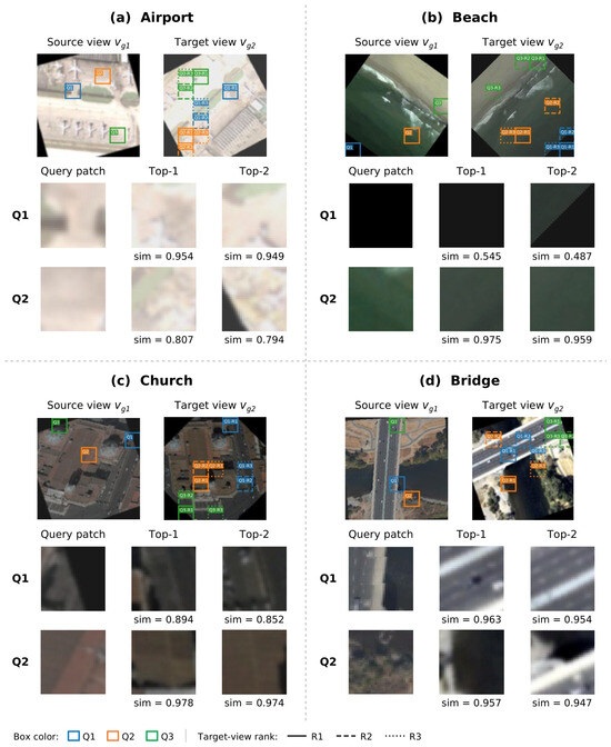
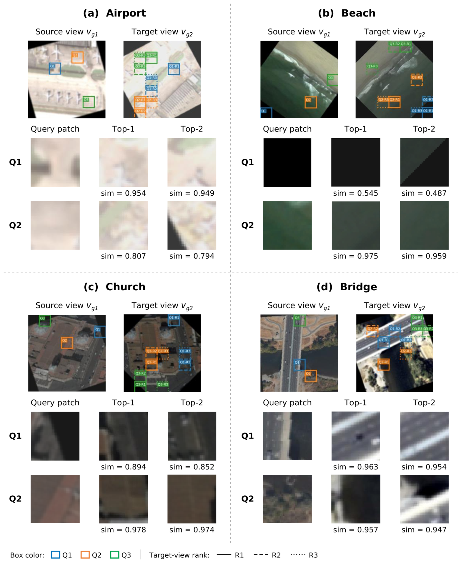
Figure 3 qualitatively illustrates the feature-neighborhood ranking behavior of C-PAM on four representative augmented view pairs. For each pair, two query locations are selected, and the top two ranked reference patches from $v_{g2}$ are displayed. Consistent with the training procedure, the cosine ranking is computed using query features extracted from the masked view $v_m$. For visual interpretability, however, the corresponding unmasked patches from $v_{g1}$ at the same query locations are shown in the figure, since directly displaying the masked patches would obscure their image content. Only the top two neighbors are shown for readability, while the default training configuration uses $K=5$. The visualization is descriptive and illustrates feature-similarity ranking rather than verified semantic correspondence or quantitative matching accuracy.

Figure 3. Qualitative visualization of the cosine-ranking behavior of C-PAM on four representative source–target image pairs. For each pair, two query locations (Q1–Q2) are selected. The cosine ranking is computed using query features extracted from the masked view $v_m$, while the corresponding unmasked patches from $v_{g1}$ at the same locations are displayed for visual interpretability. The top two reference patches from the target view $v_{g2}$ are shown for each query. Colored boxes indicate the corresponding locations, and the values below the retrieved patches denote cosine similarities. For readability, only the top two neighbors are displayed, while the default training configuration uses $K=5$. The retrieved patches represent feature-similarity neighbors rather than verified semantic correspondences.

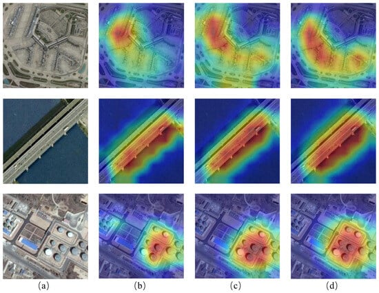
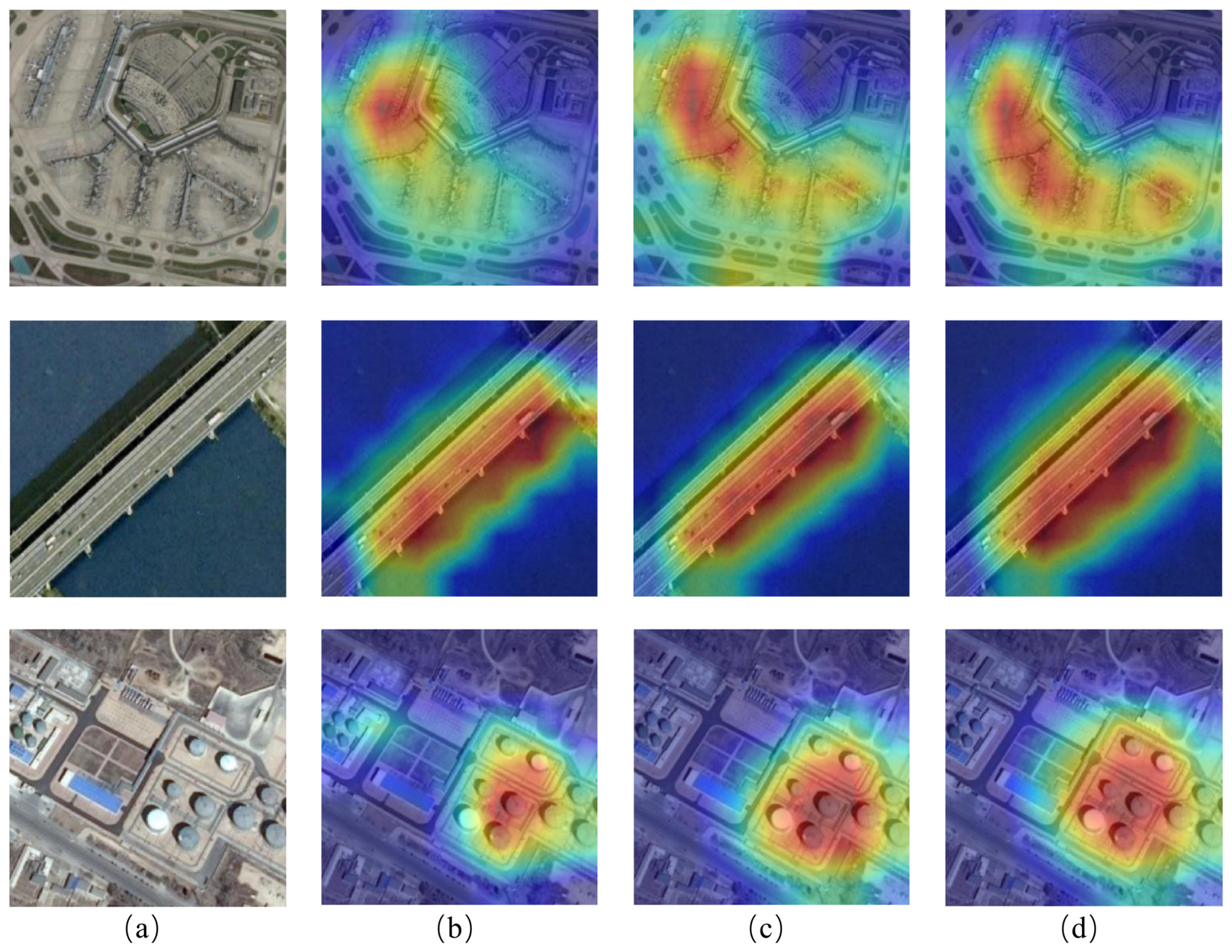
To further analyze the behavior of the learned representations, we visualize Grad-CAM activation maps under different low-label settings on the AID dataset. As shown in Figure 4, column (a) shows the original remote sensing images, while columns (b), (c), and (d) present the Grad-CAM maps obtained using labeled training subsets containing 1%, 5%, and 10% of the training partition, respectively.

Figure 4. Grad-CAM visualizations under different low-label settings on the AID dataset. Column (a) shows the original remote sensing images, while columns (b–d) show the Grad-CAM maps obtained using labeled training subsets containing 1%, 5%, and 10% of the training partition, respectively.

The visualization results indicate that the model can attend to semantically meaningful regions related to scene categories. In the airport example, the activation covers the central airport facilities and becomes more structured as the proportion of labeled samples increases. For the bridge scene, the response remains concentrated along the elongated bridge structure rather than spreading over the surrounding water area. In the storage-tank example, the activation increasingly focuses on the tank cluster and suppresses less informative background regions. These cases are relevant because the discriminative evidence is distributed differently across scene types: an airport depends on a broader spatial layout, whereas bridges and storage tanks are identified by more localized structures.

The activation maps are already category-relevant in the 1% setting and become more concentrated in the 5% and 10% settings. This observation is consistent with the quantitative low-label results. The maps remain category-relevant when the downstream classifier receives limited supervision, while additional labels refine the localization of the most informative regions.

4.4. Ablation Study

We conduct ablation studies to examine the contribution of each component in the proposed framework. Starting from the contrastive baseline using only ${\mathcal{L}}_{\mathrm{con}}$, we progressively introduce the masked reconstruction loss ${\mathcal{L}}_{\mathrm{rec}}$ and the proposed C-PAM loss ${\mathcal{L}}_{\mathrm{cpam}}$. The results under the linear probing protocol are summarized in Table 6.

On AID, the contrastive baseline achieves 95.53% accuracy and mainly captures scene-level semantic invariance. Adding masked reconstruction increases the accuracy to 96.27%, an improvement of 0.74 percentage points. This result indicates that recovering masked regions helps preserve local structural information that is not fully captured by image-level contrastive learning. Adding C-PAM to the contrastive baseline produces an improvement of 0.99 percentage points, reaching 96.52%. Patch-level feature alignment therefore increases accuracy even without the reconstruction loss.

The full model reaches 97.14%, improving the contrastive baseline by 1.61 percentage points. It also exceeds the reconstruction-only extension by 0.87 percentage points and the C-PAM-only extension by 0.62 percentage points. This pattern shows that masked reconstruction and C-PAM provide complementary contributions. Reconstruction encourages the encoder to retain local content from incomplete observations, while C-PAM encourages local features to remain consistent and discriminative across views. Their combination achieves a higher accuracy than either local objective alone.

A similar trend is observed on NWPU-RESISC45. The contrastive baseline achieves 93.84% accuracy. Adding masked reconstruction or C-PAM individually increases the accuracy to 94.92% and 95.26%, respectively, corresponding to gains of 1.08 and 1.42 percentage points. The full model reaches 96.13%, outperforming the contrastive baseline by 2.29 percentage points and the variants with only masked reconstruction or only C-PAM added by 1.21 and 0.87 percentage points, respectively. These results further support the complementary contributions of the two local objectives across the two evaluated datasets.

• Hyperparameter sensitivity.

The sensitivity analysis of key hyperparameters is summarized in Table 7.

Table 7. Sensitivity analysis of key hyperparameters in CoGLoR. Linear probing accuracy (%) is reported on the AID dataset using the 50% training split.

Hyperparameter	Setting	Linear Acc. (%)
Mask ratio	0.30	96.48 ± 0.18
Mask ratio	0.50	97.02 ± 0.17
Mask ratio	0.75	97.14 ± 0.16
Mask ratio	0.90	96.61 ± 0.20
C-PAM weight ${\lambda }_{\mathrm{cpam}}$	0.1	96.75 ± 0.19
C-PAM weight ${\lambda }_{\mathrm{cpam}}$	0.5	97.14 ± 0.16
C-PAM weight ${\lambda }_{\mathrm{cpam}}$	1.0	96.89 ± 0.18
C-PAM temperature ${\tau }_{\mathrm{pam}}$	0.07	96.92 ± 0.18
C-PAM temperature ${\tau }_{\mathrm{pam}}$	0.10	97.14 ± 0.16
C-PAM temperature ${\tau }_{\mathrm{pam}}$	0.20	96.84 ± 0.19

The mask-ratio results show a clear trade-off between reconstruction difficulty and information availability. Increasing the mask ratio from 0.30 to 0.50 improves accuracy from 96.48% to 97.02%, and a ratio of 0.75 yields the best result of 97.14%. A moderately high mask ratio forces the encoder to infer missing structures from broader context instead of relying on local appearance alone. However, increasing the ratio to 0.90 reduces accuracy to 96.61%, indicating that excessive masking removes too many informative regions and weakens the quality of local correspondence learning.

The C-PAM weight exhibits a similar balance. A value of ${\lambda }_{\mathrm{cpam}}=0.1$ yields 96.75%, while the default value of 0.5 improves accuracy to 97.14%. Increasing the weight to 1.0 reduces accuracy to 96.89%. Among the tested settings, ${\lambda }_{\mathrm{cpam}}=0.5$ provides the best balance. For the C-PAM temperature, ${\tau }_{\mathrm{pam}}=0.10$ achieves the best result.

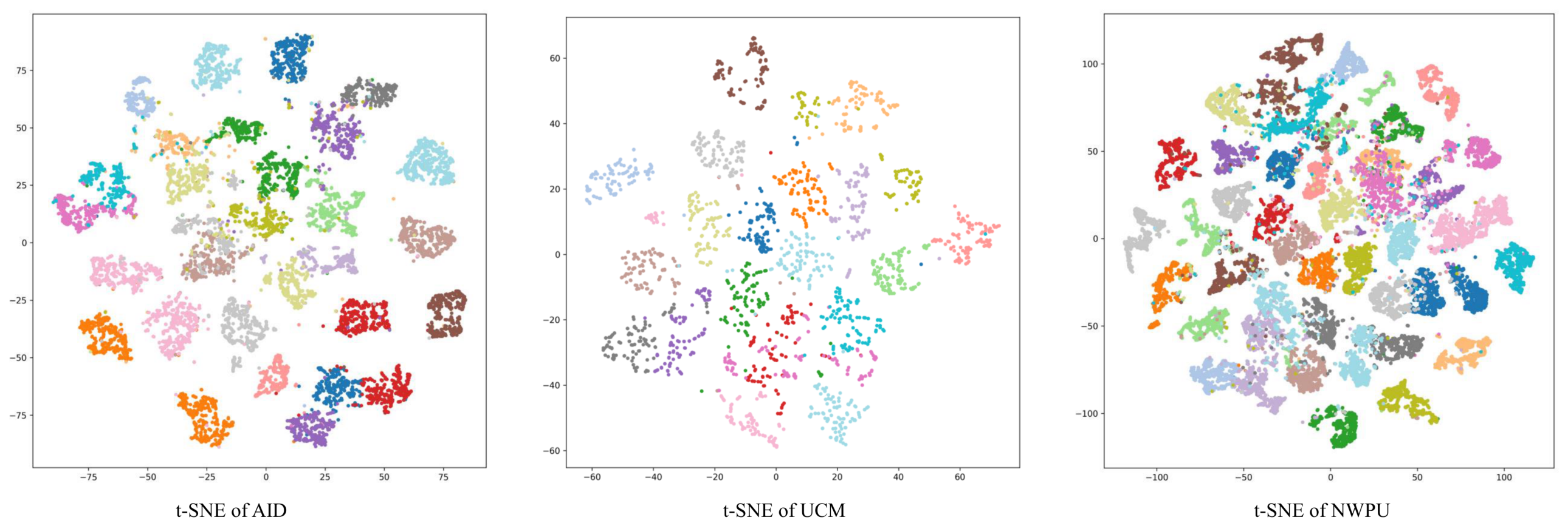
To further evaluate the learned representations, we visualize the feature embeddings of the test samples using t-SNE [43]. As shown in Figure 5, the embeddings on AID and UCM contain many compact and well-separated groups. The NWPU-RESISC45 visualization is more crowded, which is consistent with the larger number of categories and the greater visual diversity of this benchmark. Numerous class-specific clusters remain distinguishable.

Figure 5. t-SNE visualization of features learned by CoGLoR on the AID, UCM, and NWPU-RESISC45 datasets. Many samples form compact class-specific groups, while the denser NWPU-RESISC45 distribution reflects its greater category diversity.

4.4.1. C-PAM Mechanism and Neighborhood-Size Ablations

Table 8 examines positive selection, the patch-level objective, and stop-gradient in C-PAM on AID and NWPU-RESISC45. Each variant changes only the specified component from the default configuration.

Table 8. Ablation studies of the C-PAM matching mechanism on AID and NWPU-RESISC45. Each variant changes only the specified component from the default configuration. Linear probing OA (%) is reported as mean ± standard deviation over repeated runs. The $K=1$ setting corresponds to single-positive matching, while the default $K=5$ setting uses multiple positive neighbors.

Block	Variant/Setting	AID	NWPU-RESISC45
Default	Top-K C-PAM, $K=5$	97.14 ± 0.16	96.13 ± 0.17
Positive selection	Fixed-index alignment	96.04 ± 0.38	94.61 ± 0.32
Positive selection	Single-positive C-PAM ($K=1$)	96.82 ± 0.34	95.57 ± 0.29
Objective	Top-K feature regression	96.58 ± 0.17	95.21 ± 0.23
Objective	C-PAM w/o batch-level negatives	96.45 ± 0.28	95.37 ± 0.35
Gradient	C-PAM w/o stop-gradient	96.76 ± 0.24	95.58 ± 0.29

The default multi-positive configuration ($K=5$) achieves 97.14% and 96.13% OA on AID and NWPU-RESISC45, respectively. Fixed-index alignment yields 96.04% and 94.61%, while single-positive C-PAM ($K=1$) reaches 96.82% and 95.57%. The default therefore improves over fixed-index alignment by 1.10 and 1.52 percentage points and over single-positive matching by 0.32 and 0.56 percentage points, respectively. These results support feature-based neighbor selection and the use of multiple positives in the evaluated settings.

Replacing the contrastive objective with top-K feature regression reduces OA to 96.58% on AID and 95.21% on NWPU-RESISC45. Removing batch-level negatives gives 96.45% and 95.37%, respectively, supporting their contribution to patch-level discrimination. Removing stop-gradient yields 96.76% and 95.58%, corresponding to decreases of 0.38 and 0.55 percentage points from the default. The consistent direction of these changes across both datasets supports the default design, although the reported OA values alone do not establish the underlying optimization mechanism.

Table 9 shows that the default contrastive C-PAM configuration with $F_{g2}$ and $K=5$ reaches 97.14% OA on AID, compared with 96.04% for fixed-index alignment and 96.58% for top-K feature regression. Using $F_{g1}$ or both $F_{g1}$ and $F_{g2}$ gives 96.63% and 96.94%, respectively. The tested alternatives $K\in \{1,3,7,9\}$ range from 96.79% to 97.03%; thus, $K=5$ is best only among the reported settings.

Table 9. Ablation studies of the C-PAM matching mechanism, reference-view selection, and neighborhood size K on AID. Each variant changes only the specified component from the default configuration. Linear probing OA is reported as mean ± standard deviation over repeated runs.

Block	Variant/Setting	Linear OA (%)
Default	Top-K C-PAM, $F_{g2}$, $K=5$	97.14 ± 0.16
Matching rule	Fixed-index alignment	96.04 ± 0.38
Matching rule	Top-K feature regression	96.58 ± 0.17
Reference view	$F_{g1}$	96.63 ± 0.32
Reference view	$F_{g1},F_{g2}$	96.94 ± 0.28
K sensitivity	$K=1$	96.82 ± 0.34
K sensitivity	$K=3$	97.03 ± 0.17
K sensitivity	$K=7$	96.98 ± 0.25
K sensitivity	$K=9$	96.79 ± 0.30

4.4.2. Computational Cost

Table 10 compares the pretraining cost of different components under the same local measurement setup. The global contrastive baseline contains 27.97 M trainable parameters and requires 8.18 GFLOPs. Adding the reconstruction branch increases the parameters to 30.59 M and the computational cost to 13.25 GFLOPs, with 1.55× peak memory and 1.62× training time per epoch. C-PAM introduces no additional trainable parameters and results in 12.59 GFLOPs, 1.45× peak memory, and 1.54× training time. The full CoGLoR model requires 30.59 M trainable parameters and 13.57 GFLOPs, corresponding to 1.65× peak memory and 1.66× training time. These results quantify the added pretraining overhead relative to the global-only configuration. After pretraining, the projection head, reconstruction decoder, and C-PAM computations are discarded, as illustrated in Figure 1; no measured inference-latency advantage is claimed.

Table 10. Relative pretraining resource comparison under the same local measurement setup. Peak memory and time per epoch are normalized to the global contrastive baseline.

Variant	Trainable Params	Pretrain GFLOPs	Peak Memory	Time/Epoch
Global contrast only	27.97 M	8.18	$1.00\times$	$1.00\times$
+Reconstruction	30.59 M	13.25	$1.55\times$	$1.62\times$
+C-PAM	27.97 M	12.59	$1.45\times$	$1.54\times$
Full CoGLoR	30.59 M	13.57	$1.65\times$	$1.66\times$

5. Discussion

5.1. Analysis of Collaborative Global–Local Learning

The experimental results show accuracy improvements when global and local learning objectives are combined. Remote sensing scenes are usually characterized by both holistic spatial layouts and local discriminative regions. For example, categories such as airports, harbors, industrial areas, and residential areas are determined not only by global land-use patterns, but also by local objects and structures. Therefore, relying only on image-level semantic invariance or local reconstruction is insufficient for learning comprehensive scene representations.

In the proposed framework, the three objectives provide complementary supervision. The global contrastive loss encourages the encoder to learn augmentation-invariant scene-level semantics and improves the separability of different scene categories. The masked reconstruction loss forces the encoder to preserve local structural information by reconstructing missing patches from partially observed inputs. The C-PAM loss further links these levels through cross-view feature-neighborhood positives. This design allows local representations to be optimized not only for reconstruction, but also for cross-view consistency and discrimination.

The ablation results further support this interpretation. Introducing masked reconstruction improves the contrastive baseline, indicating that local structural modeling contributes useful information to scene representation. Adding C-PAM further improves accuracy beyond the parallel combination of contrastive learning and reconstruction. Under random cropping, C-PAM selects feature neighbors according to similarity rather than fixed spatial positions. Its contrastive formulation uses batch-level patch candidates for patch-level discrimination.

5.2. Role of C-PAM in Remote Sensing Representation Learning

The proposed C-PAM module addresses two issues that are particularly relevant to remote sensing images. First, strong spatial augmentations may destroy the spatial correspondence between two views. In this case, aligning features at the same patch index can introduce noisy supervision. C-PAM avoids this problem by searching for top-K similar feature tokens from the corresponding unmasked view. As a result, the alignment process becomes less dependent on absolute spatial coordinates and more dependent on learned feature content.

Second, local regions in remote sensing images often contain repeated or visually similar structures, such as roads, buildings, vegetation, and water areas. Directly regressing a masked patch feature to a single matched feature may provide weak supervision, especially when the selected patches are already highly similar. C-PAM reformulates patch matching as a contrastive objective, where the top-K matched patches are treated as positive candidates and batch-level patch features are used as a contrastive normalization set. This formulation introduces a discriminative patch-level constraint and encourages the model to identify high-similarity feature neighbors across views.

This mechanism is also consistent with the characteristics of remote sensing scene classification. Important local regions, such as aircraft in airport scenes, ships in harbor scenes, or storage tanks in industrial scenes, may occupy only a small portion of the image but provide informative category cues. By repeatedly matching and contrasting patch-level representations across views, C-PAM helps the encoder learn local features that are coordinated with the global scene context.

Figure 3 qualitatively illustrates the cosine-ranking behavior, whereas Table 9 quantitatively compares matching rules, reference views, and neighborhood sizes. The visualization does not establish semantic correctness: feature similarity is model-dependent, and the selected tokens are training neighbors rather than verified semantic identities.

5.3. Relationship to Closest Prior Work

DenseCL and VICRegL establish that dense/local correspondence predates C-PAM [10,33], while CMAE and CMID already combine discriminative and masked or global–local objectives [32,35]. CoGLoR therefore does not claim novelty for hybrid global–local SSL itself. The narrower contribution is the hard top-K, multi-positive, batch-contrastive rule evaluated with a masked CNN feature map, together with qualitative ranking visualizations and controlled matching-rule and remote sensing experiments.

5.4. Limitations and Future Work

The current study has several limitations. First, the current framework is mainly evaluated on RGB scene classification datasets. Remote sensing data may also include multispectral, hyperspectral, SAR, and multi-temporal imagery, where the relationship between global semantics and local structures can be more complex. These modalities are also relevant to site-specific monitoring problems; for example, time-series InSAR has been applied to permafrost-related surface-deformation monitoring at Tiksi Airport [44]. Extending the proposed collaborative global–local learning strategy to these data modalities is an important direction for future work.

Second, C-PAM introduces additional patch-level similarity computation during pretraining. Its computational cost increases with batch size and the number of patch tokens. More efficient patch sampling, memory-bank construction, or approximate matching strategies could further improve training efficiency.

Third, the current method focuses on scene-level classification. Future work will evaluate the learned patch-level feature representations on downstream remote sensing tasks such as semantic segmentation, object detection, and change detection.

The added ViT-S/16 experiment tests only one transformer configuration, and the K-sensitivity result does not establish robustness beyond the tested range. Accordingly, the conclusions remain limited to RGB scene classification and the evaluated backbones.

Overall, the results support explicit collaboration between global semantic learning, local reconstruction, and contrastive patch-level alignment for self-supervised remote sensing representation learning.

6. Conclusions

This paper proposes CoGLoR, a collaborative global–local self-supervised learning framework for remote sensing scene classification. The proposed method integrates global contrastive learning, masked reconstruction, and Contrastive Patch-Level Attention Matching (C-PAM) within a unified training pipeline. The contrastive branch learns scene-level semantic invariance from augmented views, the reconstruction branch preserves local structural information by recovering masked patches, and the C-PAM branch uses a hard top-K feature neighborhood as a multi-positive contrastive set.

Experimental results on remote sensing scene classification benchmarks show that CoGLoR improves over the compared baselines under linear probing and low-label evaluation protocols. The ablation studies further show that global contrastive learning, masked reconstruction, and C-PAM provide complementary supervision. In particular, C-PAM reduces spatial mismatch caused by random cropping and introduces contrastive patch-level feature discrimination.

Overall, the results support explicit collaboration between global semantic learning and local structural modeling for self-supervised remote sensing representation learning. Future work will explore the extension of this framework to more diverse remote sensing modalities and downstream tasks, such as multispectral imagery, semantic segmentation, object detection, and change detection.

The claims are restricted to the evaluated RGB scene-classification settings. The results across three datasets and the evaluated ResNet-50 and ViT-S/16 configurations are treated as bounded evaluations rather than evidence of universal transfer, and feature similarity is not treated as verified semantic identity.

References

- Cheng, G.; Han, J.; Lu, X. Remote sensing image scene classification: Benchmark and state of the art. Proc. IEEE 2017, 105, 1865–1883. [Google Scholar] [CrossRef] [Scilit]
- Thapa, A.; Horanont, T.; Neupane, B.; Aryal, J. Deep Learning for Remote Sensing Image Scene Classification: A Review and Meta-Analysis. Remote Sens. 2023, 15, 4804. [Google Scholar] [CrossRef] [Scilit]
- Li, X.; Yang, X.; Zhang, Z.; Zhai, J.; Meng, X. Evaluating of ground surface freeze–thaw and the interrelationship with vegetation cover on the Qinghai-Xizang Plateau. Geoderma 2025, 453, 117141. [Google Scholar] [CrossRef] [Scilit]
- Cheng, G.; Yang, C.; Yao, X.; Guo, L.; Han, J. When deep learning meets metric learning: Remote sensing image scene classification via learning discriminative CNNs. IEEE Trans. Geosci. Remote Sens. 2018, 56, 2811–2821. [Google Scholar] [CrossRef] [Scilit]
- Bazi, Y.; Bashmal, L.; Al Rahhal, M.M.; Al Dayil, R.; Al Ajlan, N. Vision transformers for remote sensing image classification. Remote Sens. 2021, 13, 516. [Google Scholar] [CrossRef] [Scilit]
- Li, X.; Zhang, Z.; Zheleznyak, M.; Jin, H.; Zhang, S.; Wei, H.; Zhai, J.; Melnikov, A.; Gagarin, L. Time-series InSAR monitoring of surface deformation in Yakutsk, a city located on continuous permafrost. Earth Surf. Process. Landf. 2024, 49, 918–932. [Google Scholar] [CrossRef] [Scilit]
- Gui, J.; Chen, T.; Zhang, J.; Cao, Q.; Sun, Z.; Luo, H.; Tao, D. A survey on self-supervised learning: Algorithms, applications, and future trends. IEEE Trans. Pattern Anal. Mach. Intell. 2024, 46, 9052–9071. [Google Scholar] [CrossRef] [Scilit] [PubMed]
- Chen, T.; Kornblith, S.; Norouzi, M.; Hinton, G. A simple framework for contrastive learning of visual representations. In International Conference on Machine Learning; PmLR: Cambridge, MA, USA, 2020; pp. 1597–1607. [Google Scholar]
- He, K.; Fan, H.; Wu, Y.; Xie, S.; Girshick, R. Momentum contrast for unsupervised visual representation learning. In IEEE/CVF Conference on Computer Vision and Pattern Recognition; IEEE: New York, NY, USA, 2020; pp. 9729–9738. [Google Scholar]
- Wang, X.; Zhang, R.; Shen, C.; Kong, T.; Li, L. Dense Contrastive Learning for Self-Supervised Visual Pre-Training. In IEEE/CVF Conference on Computer Vision and Pattern Recognition; IEEE: New York, NY, USA, 2021; pp. 3024–3033. [Google Scholar]
- Chen, X.; He, K. Exploring simple siamese representation learning. In IEEE/CVF Conference on Computer Vision and Pattern Recognition; IEEE: New York, NY, USA, 2021; pp. 15750–15758. [Google Scholar]
- He, K.; Chen, X.; Xie, S.; Li, Y.; Dollár, P.; Girshick, R. Masked autoencoders are scalable vision learners. In IEEE/CVF Conference on Computer Vision and Pattern Recognition; IEEE: New York, NY, USA, 2022; pp. 16000–16009. [Google Scholar]
- Bao, H.; Dong, L.; Piao, S.; Wei, F. BEiT: BERT Pre-Training of Image Transformers. In International Conference on Learning Representations; PmLR: Cambridge, MA, USA, 2022. [Google Scholar]
- Xie, Z.; Zhang, Z.; Cao, Y.; Lin, Y.; Bao, J.; Yao, Z.; Dai, Q.; Hu, H. SimMIM: A Simple Framework for Masked Image Modeling. In IEEE/CVF Conference on Computer Vision and Pattern Recognition; IEEE: New York, NY, USA, 2022; pp. 9653–9663. [Google Scholar]
- Bi, Q.; Qin, K.; Li, Z.; Zhang, H.; Xu, K.; Xia, G.S. A multiple-instance densely-connected ConvNet for aerial scene classification. IEEE Trans. Image Process. 2020, 29, 4911–4926. [Google Scholar] [CrossRef] [Scilit] [PubMed]
- Bi, Q.; Qin, K.; Zhang, H.; Xia, G.S. Local semantic enhanced ConvNet for aerial scene recognition. IEEE Trans. Image Process. 2021, 30, 6498–6511. [Google Scholar] [CrossRef] [Scilit] [PubMed]
- Bi, Q.; Zhou, B.; Qin, K.; Ye, Q.; Xia, G.S. All grains, one scheme (AGOS): Learning multigrain instance representation for aerial scene classification. IEEE Trans. Geosci. Remote Sens. 2022, 60, 5629217. [Google Scholar] [CrossRef] [Scilit]
- Long, Y.; Xia, G.S.; Li, S.; Yang, W.; Yang, M.Y.; Zhu, X.X.; Zhang, L.; Li, D. On creating benchmark dataset for aerial image interpretation: Reviews, guidances, and Million-AID. IEEE J. Sel. Top. Appl. Earth Obs. Remote Sens. 2021, 14, 4205–4230. [Google Scholar] [CrossRef] [Scilit]
- Zhao, Z.; Luo, Z.; Li, J.; Chen, C.; Piao, Y. When Self-Supervised Learning Meets Scene Classification: Remote Sensing Scene Classification Based on a Multitask Learning Framework. Remote Sens. 2020, 12, 3276. [Google Scholar] [CrossRef] [Scilit]
- Berg, P.; Pham, M.T.; Courty, N. Self-Supervised Learning for Scene Classification in Remote Sensing: Current State of the Art and Perspectives. Remote Sens. 2022, 14, 3995. [Google Scholar] [CrossRef] [Scilit]
- Chen, X.; Zhu, G.; Liu, M. Remote Sensing Image Scene Classification with Self-Supervised Learning Based on Partially Unlabeled Datasets. Remote Sens. 2022, 14, 5838. [Google Scholar] [CrossRef] [Scilit]
- Yu, Y.; Li, X.; Liu, F. Attention GANs: Unsupervised deep feature learning for aerial scene classification. IEEE Trans. Geosci. Remote Sens. 2020, 58, 519–531. [Google Scholar] [CrossRef] [Scilit]
- Li, X.; Shi, D.; Diao, X.; Xu, H. SCL-MLNet: Boosting few-shot remote sensing scene classification via self-supervised contrastive learning. IEEE Trans. Geosci. Remote Sens. 2022, 60, 5801112. [Google Scholar] [CrossRef] [Scilit]
- Gao, Y.; Sun, X.; Liu, C. A General Self-Supervised Framework for Remote Sensing Image Classification. Remote Sens. 2022, 14, 4824. [Google Scholar] [CrossRef] [Scilit]
- Zhang, X.; Han, L. A Generic Self-Supervised Learning (SSL) Framework for Representation Learning from Spectral–Spatial Features of Unlabeled Remote Sensing Imagery. Remote Sens. 2023, 15, 5238. [Google Scholar] [CrossRef] [Scilit]
- Mañas, O.; Lacoste, A.; Giró-i Nieto, X.; Vazquez, D.; Rodríguez, P. Seasonal Contrast: Unsupervised Pre-Training from Uncurated Remote Sensing Data. In IEEE/CVF International Conference on Computer Vision; IEEE: New York, NY, USA, 2021; pp. 9414–9423. [Google Scholar]
- Cong, Y.; Khanna, S.; Meng, C.; Liu, P.; Rozi, E.; He, Y.; Burke, M.; Lobell, D.; Ermon, S. SatMAE: Pre-training Transformers for Temporal and Multi-Spectral Satellite Imagery. In Proceedings of the Advances in Neural Information Processing Systems, New Orleans, LA, USA, 28 November–9 December 2022; Volume 35. [Google Scholar]
- Kang, J.; Fernandez-Beltran, R.; Duan, P.; Liu, S.; Plaza, A.J. Deep Unsupervised Embedding for Remotely Sensed Images Based on Spatially Augmented Momentum Contrast. IEEE Trans. Geosci. Remote Sens. 2021, 59, 2598–2610. [Google Scholar] [CrossRef] [Scilit]
- Huang, H.; Mou, Z.; Li, Y.; Li, Q.; Chen, J.; Li, H. Spatial-Temporal Invariant Contrastive Learning for Remote Sensing Scene Classification. IEEE Geosci. Remote Sens. Lett. 2022, 19, 6509805. [Google Scholar] [CrossRef] [Scilit]
- Zhou, J.; Wei, C.; Wang, H.; Shen, W.; Xie, C.; Yuille, A.; Kong, T. IBOT: Image BERT Pre-Training with Online Tokenizer. In International Conference on Learning Representations; PmLR: Cambridge, MA, USA, 2022. [Google Scholar]
- Assran, M.; Caron, M.; Misra, I.; Bojanowski, P.; Bordes, F.; Vincent, P.; Joulin, A.; Rabbat, M.; Ballas, N. Masked Siamese Networks for Label-Efficient Learning. In Computer Vision—ECCV 2022; Springer: Berlin/Heidelberg, Germany, 2022; pp. 456–473. [Google Scholar] [CrossRef] [Scilit]
- Huang, Z.; Jin, X.; Lu, C.; Hou, Q.; Cheng, M.M.; Fu, D.; Shen, X.; Feng, J. Contrastive Masked Autoencoders Are Stronger Vision Learners. IEEE Trans. Pattern Anal. Mach. Intell. 2024, 46, 2506–2517. [Google Scholar] [CrossRef] [Scilit] [PubMed]
- Bardes, A.; Ponce, J.; LeCun, Y. VICRegL: Self-Supervised Learning of Local Visual Features. In Proceedings of the Advances in Neural Information Processing Systems, New Orleans, LA, USA, 28 November–9 December 2022; Volume 35. [Google Scholar]
- Tao, C.; Zhu, X.; Su, W.; Huang, G.; Li, B.; Zhou, J.; Qiao, Y.; Wang, X.; Dai, J. Siamese Image Modeling for Self-Supervised Vision Representation Learning. In IEEE/CVF Conference on Computer Vision and Pattern Recognition; IEEE: New York, NY, USA, 2023; pp. 2132–2141. [Google Scholar]
- Muhtar, D.; Zhang, X.; Xiao, P.; Li, Z.; Gu, F. CMID: A Unified Self-Supervised Learning Framework for Remote Sensing Image Understanding. IEEE Trans. Geosci. Remote Sens. 2023, 61, 5607817. [Google Scholar] [CrossRef] [Scilit]
- Reed, C.; Gupta, R.; Li, S.; Brockman, S.; Funk, C.; Clipp, B.; Keutzer, K.; Candido, S.; Uyttendaele, M.; Darrell, T. Scale-MAE: A Scale-Aware Masked Autoencoder for Multiscale Geospatial Representation Learning. In IEEE/CVF International Conference on Computer Vision; IEEE: New York, NY, USA, 2023; pp. 4088–4099. [Google Scholar]
- Oquab, M.; Darcet, T.; Moutakanni, T.; Vo, H.; Szafraniec, M.; Khalidov, V.; Fernandez, P.; Haziza, D.; Massa, F.; El-Nouby, A.; et al. DINOv2: Learning Robust Visual Features without Supervision. In Transactions on Machine Learning Research; TMLR: New York, NY, USA, 2024. [Google Scholar]
- Pang, S.; Xiang, J.; Zuo, Z.; Hu, H.; Jiang, H. CMFM: A Contrastive Masked Feature Modeling Framework for Remote Sensing Image Semantic Segmentation. Remote Sens. 2026, 18, 626. [Google Scholar] [CrossRef] [Scilit]
- Oord, A.v.d.; Li, Y.; Vinyals, O. Representation learning with contrastive predictive coding. arXiv 2018, arXiv:1807.03748. [Google Scholar]
- Xia, G.S.; Hu, J.; Hu, F.; Shi, B.; Bai, X.; Zhong, Y.; Zhang, L.; Lu, X. AID: A benchmark data set for performance evaluation of aerial scene classification. IEEE Trans. Geosci. Remote Sens. 2017, 55, 3965–3981. [Google Scholar] [CrossRef] [Scilit]
- Yang, Y.; Newsam, S. Bag-of-visual-words and spatial extensions for land-use classification. In 18th SIGSPATIAL International Conference on Advances in Geographic Information Systems; ACM: New York, NY, USA, 2010; pp. 270–279. [Google Scholar] [CrossRef] [Scilit]
- He, K.; Zhang, X.; Ren, S.; Sun, J. Deep residual learning for image recognition. In IEEE Conference on Computer Vision and Pattern Recognition; IEEE: New York, NY, USA, 2016; pp. 770–778. [Google Scholar]
- Maaten, L.v.d.; Hinton, G. Visualizing data using t-SNE. J. Mach. Learn. Res. 2008, 9, 2579–2605. [Google Scholar] [CrossRef] [Scilit]
- Yan, Q.; Zhang, Z.; Li, X.; Yan, A.; Qiu, L.; Zhang, A.; Melnikov, A.; Gagarin, L. Time-Series InSAR Monitoring of Permafrost-Related Surface Deformation at Tiksi Airport: Impacts of Climate Warming and Coastal Erosion on the Northernmost Siberian Mainland. Remote Sens. 2025, 17, 1757. [Google Scholar] [CrossRef] [Scilit]
Disclaimer/Publisher’s Note: The statements, opinions and data contained in all publications are solely those of the individual author(s) and contributor(s) and not of MDPI and/or the editor(s). MDPI and/or the editor(s) disclaim responsibility for any injury to people or property resulting from any ideas, methods, instructions or products referred to in the content. |
© 2026 by the authors. Licensee MDPI, Basel, Switzerland. This article is an open access article distributed under the terms and conditions of the Creative Commons Attribution (CC BY) license.