GT-LandSDS: A Novel Spatiotemporal Integrated Framework for Land Use Simulation by Coupling Cellular Automata with Graph Attention Network and Transformer

Highlights

What are the main findings?

• A coupled GAT-Transformer-LandSDS (GT-LandSDS) architecture was proposed to jointly model spatial dependencies and temporal dynamics for land use change simulation.
• A graph attention network served as the spatial encoder to resolve higher-order inter-parcel relationships, while a transformer captured cross-time change patterns from available multi-period observations.

What is the implication of the main finding?

• Multi-scenario simulations reveal distinct spatial patterns of urban expansion under varying policy interventions, providing critical insights for balancing economic growth with ecological conservation in fragile karst environments.
• This framework provides a scientific and feasible approach for simulating large-scale, long-term land use patterns by coupling deep learning with cellular automata.

Abstract

To address the limitation of traditional cellular automata models in effectively integrating temporal and spatial information, this study extends the previously developed Land use Simulation and Decision-Support system (LandSDS). By incorporating a graph attention network (GAT), a transformer, and an agent-based model (ABM) into a cellular automata framework informed by remote sensing time series, GT-LandSDS is constructed. Specifically, GAT dynamically captures higher-order spatial dependencies among land parcels; the self-attention mechanism of the transformer extracts land use change characteristics from multi-period observations; and ABM captures human behavioral decisions of three types, namely traffic, resident, and government. Based on this framework, GT-LandSDS derives CA transition rules from multiple dimensions and enhances the dynamic exploration of land use change across space and time. Using Guangxi Zhuang Autonomous Region as a case study, the model was validated with remote sensing land use data from six periods (2000, 2005, 2010, 2015, 2020, and 2023), and scenario-based future predictions were generated. The results show that: (1) The overall accuracy reaches 0.926, while the Kappa coefficient is 0.820, and the figure of merit (FoM) for change simulation is 0.034, indicating a relative advantage over ANN-CA, LSTM-CA, and UESP in overall pattern simulation, although fine-scale change reproduction remains limited; (2) Three development scenarios were then assessed: continuing historical trends, theoretical high-intensity urban expansion, and karst landform conservation under a green transformation development policy. The land use pattern of the area from 2023 to 2035 was predicted. The findings reveal that accelerating urbanization leads to rapid expansion of construction land, increasing by more than 88% compared with 2023, and causes substantial cropland loss. In contrast, intervention through the green transformation development policy limits construction land growth to 26.5%, effectively curbing urban sprawl while protecting forest, grassland, and cropland resources in the karst landscape. This study offers new insights into land use change simulation in ecologically fragile regions subject to strong policy interventions. It provides a scientific basis for coordinating ecological conservation and high-quality development in karst areas.

1. Introduction

Cities are key carriers of modernization and essential spaces for human well-being [1]. Urban expansion mainly appears as outward growth along dominant directions, such as major transportation corridors and industrial belts, or rapid spread from inner areas to the periphery [2,3]. These phenomena have become important research topics in geography, socioeconomics, ecology, environmental science, and GIScience [2,4]. In recent years, China’s urbanization has entered a more stable stage, and urban development has shifted toward revitalizing and optimizing existing built-up stock. Consequently, promoting the green transformation of urban development [1] has become an important issue in urban expansion simulation research [5].

Compared with empirical models, dynamic simulation frameworks such as cellular automata (CA) have been widely used in urban expansion simulation because of their high degree of automation [6,7]. A CA model consists of five components: cells, cell states, cell space, neighborhoods, and transition rules. It simulates the spatial process of urban expansion through local neighborhood interactions [8]. However, traditional raster-based CA models have several limitations. Raster boundaries do not correspond to actual parcel boundaries, irregular land units are difficult to represent accurately, and vector geographic features such as points, lines, and polygons cannot be directly incorporated [9]. The emergence of vector cellular automata (VCA) has addressed the problems of geometric distortion and topological discontinuity caused by the discretization of continuous urban space into a homogeneous grid in raster-based CA models [10,11].

In recent years, coupling multiple models for urban expansion simulation has become increasingly mature [4]. For example, Liu et al. (2017) coupled top-down SD with bottom-up CA and introduced an artificial neural network (ANN) algorithm to develop FLUS model, which adaptively learns the development suitability probability of each land use type at each cell [12,13]. Feng and Tong (2018) proposed a cellular automata model with spatially nonstationary transition rules based on geographically weighted regression, thereby capturing local variations in land use conversion potential [14]. Liang et al. (2021) coupled the Land Expansion Analysis Strategy (LEAS) with a multi-type random patch seed CA model to build the PLUS model, which improves the inference of patch evolution capability [15]. Wu et al. (2022) proposed a multi-label CNN model (ML-CNN-CA) that assigns multiple land use types to each grid cell, which uses neighborhood effect, adaptive inertia, and a random factor to better capture mixed land use changes [16]. Our team systematically examined the strengths and limitations of SD, CA, and ABM models; achieved bidirectional real-time data communication between SD and CA models [17,18]; developed and implemented the Land-use Simulation and Decision-Support System (LandSDS); and explored the potential of multi-model integration [19,20]. These efforts laid the theoretical foundation for the research presented in this paper. Recent studies have coupled CNN, LSTM, and CA to improve the representation of spatial neighborhoods and temporal dependence in land use simulation. CNN–CA models learn nonlinear spatial features from local land use neighborhoods, while neural-network-enhanced CA–Markov models use data-driven transition-potential maps to incorporate environmental and socioeconomic factors into spatial allocation [21,22,23]. However, these models generally rely on fixed spatial windows or treat temporal demand estimation and spatial allocation as relatively separate processes.

With breakthroughs in deep learning, graph neural networks (GNNs) have revolutionized spatial relationship modeling [24], overcoming limitations in accuracy and representation in land use change simulation and becoming a major research focus [25]. Among them, the graph attention network (GAT) adaptively learns relationship weights between nodes through its attention mechanism, accurately capturing dynamic dependencies in spatial topological relationships [26]. Guan et al. (2023) developed the HGAT-VCA model based on a higher-order graph attention network, enhancing its ability to capture complex spatial dependencies by incorporating higher-order neighborhood information [27]. Guan et al. (2024) proposed the HashGAT-VCA model, which uses hash functions to improve the computational efficiency of the graph attention mechanism and further improve simulation accuracy [28]. Gao et al. (2025) introduced ABM and employed an urban expansion scenario prediction (UESP) model with GAT, ABM, and VCA, to emphasize the influence of socio-behavioral factors, such as resident preferences and government planning, on urban expansion at the micro-level [29]. Recent studies have also introduced GCNs into graph-based CA for urban growth simulation, further demonstrating the value of GNNs in LUCC modeling [30]. However, while GAT is adept at capturing spatial relationships among land parcels, it cannot account for temporal changes in parcels. Unlike CNN-based models that use fixed convolutional windows, GAT adaptively assigns different weights to neighboring spatial units and can capture higher-order topological dependencies. This provides a more flexible representation of spatial heterogeneity in land use change simulation.

Time, as a fundamental dimension in dynamic land use change modeling, is crucial for realistic urban expansion simulation because of the inherently dynamic nature of urban growth [31]. Zhou et al. (2023) integrated K-means clustering, convolutional neural networks (CNNs), and long short-term memory (LSTM) to construct the KCL-CA model, addressing temporal dependency and spatial heterogeneity [32]. Yao et al. (2024) obtained high-resolution time series at the cadastral scale, and they used the Temporal-VCA architecture to identify parcel change characteristics over short time intervals, thereby significantly improving simulation accuracy [33]. However, these models still process time series sequentially, making them prone to forgetting early information when handling multi-period land use observations. In natural language processing, Vaswani et al. (2017) proposed the transformer, which can effectively capture dependencies between any two positions in an input sequence through self-attention, thereby improving sequence-dependency modeling [34]. Compared with CA–Markov and recurrent models, the transformer can directly model relationships among different historical time steps through self-attention. Therefore, GT-LandSDS combines adaptive spatial representation through GAT, cross-time dependency modeling through transformer, and natural, socioeconomic, and policy effects through ABM and explicit spatial constraints.

To address these issues, this study introduces a temporal transformer model and a GAT model into LandSDS and constructs a coupled model within the CA framework that integrates transformer, GAT, and ABM, namely GAT-Transformer-LandSDS (GT-LandSDS). In this model, GAT captures spatial neighborhood relationships among parcels, while transformer processes global information on parcel changes across available historical observations, thereby preserving local spatial sensitivity while enhancing temporal context awareness. Furthermore, ABM is used to model the decision-making processes of government, transportation, and resident agents, aiming to improve overall pattern simulation and represent the spatiotemporal characteristics of urban expansion under multiple driving factors. Against the backdrop of a new stage of urbanization and policies promoting the green transformation of urban development, this study takes Guangxi Zhuang Autonomous Region, hereinafter referred to as Guangxi, as a case study. Three future urban expansion scenarios are designed: (1) continuation of historical trends (inertial development), (2) theoretical high-intensity urban expansion, and (3) ecological protection of karst landforms under the green transformation policy. Land use patterns in Guangxi from 2023 to 2035 are predicted to reveal spatial differences in urban expansion under policy intervention, support the formulation of policies for optimizing land use patterns, and promote regional sustainable development. Section 2 introduces the overall framework and implementation of GT-LandSDS; Section 3 presents the study area, data sources, and data acquisition; Section 4 establishes a model accuracy evaluation system, presents the results of multi-model comparison, and selects specific windows for detailed analysis of simulation performance; Section 5 develops three scenarios based on historical trends, theoretical high-intensity urban expansion, and green transformation policy intervention, and uses GT-LandSDS to predict and analyze land use changes in Guangxi from 2023 to 2035; Section 6 discusses the innovations and applications of the model; and Section 7 concludes the paper.

2. Methodology

2.1. LandSDS

LandSDS enables bidirectional data exchange between the system dynamics (SD) and CA models and incorporates an agent-based model (ABM) to capture the mechanisms of human-environment interaction. Based on the SD model, the system generates land use scenario projections in response to macro-level driving factors, such as land use and population policies. It then transmits the simulation results to the CA model, thereby controlling its iterative process at the macro-level and influencing its transition rules at the micro-level. Meanwhile, the CA model uses micro-level grid cells to integrate the complex decision-making behaviors of different agents from the ABM into the cell state transition process: resident agents select suitable residential areas based on accessibility to transportation, education, and healthcare, whereas government agents impose mandatory constraints on the land use types of specific parcels through macro-level planning. On this basis, the system feeds the indicator parameters obtained during the CA model run back into the SD model to calibrate its parameters, thereby completing the bidirectional dynamic adjustment and real-time communication between the SD and CA models. Further details are provided by Liu et al. (2020) [19].

2.2. General Structure

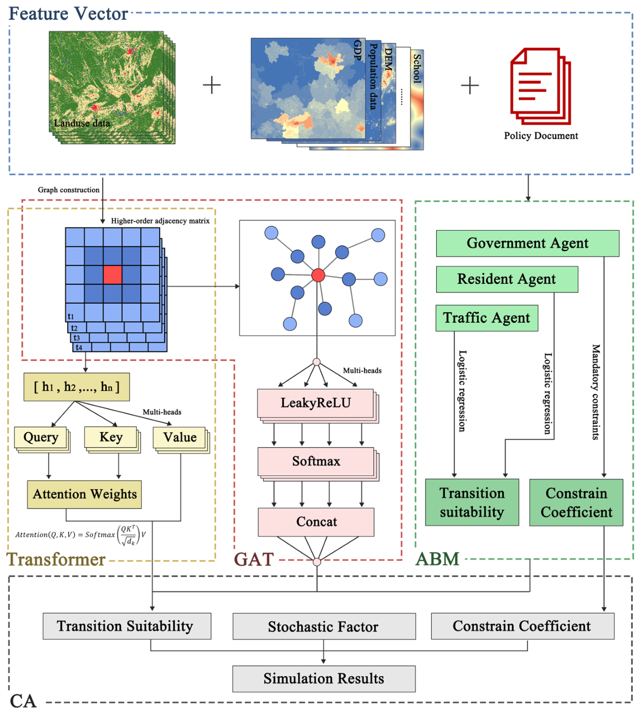
The overall architecture of the GT-LandSDS model is shown in Figure 1 and comprises three core modules:

(1) GAT: By treating vector parcels as nodes, this module constructs a higher-order neighborhood graph based on spatial proximity. A multi-head graph attention mechanism is used to dynamically capture interdependencies among parcels and quantify the influence weights of neighboring parcels on the conversion potential of the target parcel.

(2) Transformer: Its self-attention mechanism performs temporal modeling of multi-temporal spatial features derived from the available multi-period observations, extracting information on their evolution and critical change points, thereby enhancing the model’s ability to mine historical data.

(3) ABM: By integrating three types of agents, namely government, transportation, and residents, this module quantifies the impact of socioeconomic factors on parcel conversion across three levels: macro-policy constraints, infrastructure-driven forces, and residents’ micro-level preferences.

On this basis, the representational outputs of the three modules are fused into adaptive parcel conversion probabilities. Combined with stochastic perturbations and mandatory constraints, and with CA serving as the evolutionary framework, the model iteratively simulates the land use change process. This model accounts for spatial heterogeneity, temporal dependence, and social behavior, making it well suited for simulating urban expansion in complex regions with fragmented terrain and strong policy interventions.

Figure 1. Framework of the methodology.

Figure 1. Framework of the methodology.

2.3. GAT

Compared with conventional spatial models, GAT can adaptively assign different attention weights to neighboring parcels, thereby more effectively capturing the heterogeneous, nonlinear, and topology-dependent spatial interactions among vector land units. This capability enables the model to represent complex neighborhood dependencies more accurately and to better reflect the influence of surrounding parcels on land parcel conversion [27,28].

In this study, the research area is partitioned into $N$ grid cells of 1000 m × 1000 m, and the centroid of each grid cell is designated as a graph node $v_i$. For a given parcel $i$, its feature vector $g_i^t\in R^d$ is defined as specified in Equation (1).

$$\begin{array}{c}{g}_i^t=\left[L_i^t,{SH}_i,{SE}_i^{\left(1\right)},\dots ,{SE}_i^{\left(m\right)}\right]\end{array}$$

(1)

where $L_i^t$ denotes the land use type of parcel $i$ at time $t$; $S{H}_i$ represent the static intrinsic attributes of parcel $i$ (e.g., elevation, slope); $S{E}_i^{\left(k\right)}$ signifies the $k$-th environmental driving factor (e.g., Euclidean distance to roadways, hospital, schools).

To capture higher-order spatial dependencies, a second-order adjacency matrix of the graph is constructed based on spatial proximity relationships with graph node $v_i$ as the basis. A learnable linear transformation $W\in R^{F^{\prime }\times F}$ projects the features into a high-dimensional space. Subsequently, the raw attention coefficients $e_{ij}^{gat}$ between parcel $i$ and its geographic neighbor $j\in N_i$ are computed, as shown in Equation (2) [26].

$$\begin{array}{c}{e}_{ij}^{gat}=LeakyReLU\left(a^T\left[W{g}_i\Vert W{g}_j\right]\right)\end{array}$$

(2)

where $g_i$ and $g_j$ denote the feature vectors of the central parcel $i$ and its neighboring parcel $j$, respectively, and a represents the parameter vector of the attention mechanism. This coefficient reflects the spatial contribution intensity of attribute changes in neighboring parcel $j$ to the expansion potential of parcel $i$. The symbol $‘\left|\right|’$ denotes vector concatenation, which preserves the complete feature information of both the central parcel and its neighbor. The LeakyReLU activation function permits the passage of negative gradients, thereby ensuring stability during backpropagation and enabling weight updates even for neighboring parcels with low attention scores.

The attention coefficients are subsequently spatially normalized using the Softmax function, yielding the attention weight ${\alpha }_{ij}$.

$${\alpha }_{ij}={\displaystyle \frac{exp\left(e_{ij}\right)}{{\sum }_{k\in N_i}exp\left(e_{ik}\right)}}$$

(3)

Subsequently, the attention weights are applied to the linearly transformed feature vectors of the neighboring parcels and summed. To preserve the intrinsic information of the central parcel, its own transformed feature representation is also incorporated into the aggregation, as formulated in Equation (4) [26]:

$$h_i^t=\sigma \left(\sum _{j\in N_i}{\alpha }_{ij}W{g}_j^t+W_{self}{g}_i^t\right)$$

(4)

where $h_i^t$ denotes the high-order spatial feature vector of parcel $i$ at time $t$ after updating through the GAT layer, $N_i$ represents the set of neighboring parcels of $i$, and $\sigma$ is a nonlinear activation function.

In this study, a multi-head attention mechanism is adopted for the GAT module. Multiple attention heads are executed in parallel, each with an independent set of parameters $W^m$ and $a^m$, and their outputs are concatenated, as expressed in Equation (5) [26]:

$$h_i^{t^{\prime }}=|{ |}_{m=1}^M \sigma \left(\sum _{j\in N_i}{\alpha }_{ij}^m{W}^m{g}_j^t\right)$$

(5)

where ${\alpha }_{ij}^m$ denotes the normalized attention coefficient computed by the m-th attention head, and $M$ represents the total number of attention heads; in this study, $M=4$. The notation $|{ |}_{m=1}^M$ signifies the concatenation of $M$ vectors. After processing through multiple GAT layers, the final embedding vector $Z_i^{GAT}$ of parcel $i$ is obtained. Finally, a fully connected layer maps the features to the parcel land use transition probability $P_{i,C}^{gat}$.

2.4. Transformer

The transformer is a deep learning architecture based on the self-attention mechanism, originally proposed by Vaswani et al. (2017) [34]. Owing to its powerful sequence modeling capabilities, it has been widely applied across domains such as natural language processing, computer vision, and spatiotemporal modeling [34].

After undergoing GAT encoding, each parcel $i$ yields a set of spatial feature vectors $h_i^t\in R^D$ corresponding to five distinct time steps. These vectors are stacked in chronological order to form the parcel’s temporal sequence:

$$\begin{array}{c}{H}_i=\left[h_i^{t_1},h_i^{t_2},\dots ,h_i^{t_n}\right]\end{array}$$

(6)

where $n$ denotes the total number of time steps encoded by the GAT, and $t\in \left\{\mathrm{2000,2005,2010,2015,2020}\right\}$. Since transformer architecture inherently lacks awareness of temporal ordering, a learnable temporal position encoding $E\in R^{n\times D}$ must be incorporated, yielding the encoder input:

$${\tilde{H}}_i=h_i^t+E_{time}$$

(7)

Multi-head attention linearly projects ${\tilde{H}}_i$ into three distinct sets of vectors-namely, Query, Key, and Value. The correlation weights between any two time steps are subsequently computed via scaled dot-product attention. The core computation can be summarized as Equation (8) [34]:

$$\begin{array}{c}Attention\left(Q,K,V\right)=Softmax\left({\displaystyle \frac{Q{K}^T}{\sqrt{d_k}}}\right)V\end{array}$$

(8)

where $Q{K}^T$ computes the dot product between the Query and Key matrices, measuring their similarity. A higher score indicates a stronger correlation between the corresponding time steps. The term $d_k$ denotes the dimensionality of the key vectors. Since the magnitude of the dot product tends to grow proportionally with $d_k$, the result is divided by $\sqrt{d_k}$ to stabilize gradients and prevent the Softmax function from entering a saturation region characterized by vanishingly small gradients.

To enable transformer to capture multi-faceted temporal information embedded within the parcel-level time series, a multi-head attention mechanism is employed in this study. The Query, Key, and Value matrices are linearly projected h times to obtain multiple sets $Q_i$, $K_i$, and $V_i$. Each attention head is then computed in parallel, as formulated as Equation (9) [34].

$$\begin{array}{c}hea{d}_j=Attention\left(Q{W}_i^Q,K{W}_i^K,V{W}_i^V\right)\end{array}$$

(9)

where $j$ denotes the $j$-th attention head, with $j\in \left\{1,\dots ,h\right\}$; in this study, $h=4$, which is a lightweight and practical setting for transformer architectures with relatively small hidden dimensions and short temporal sequences [34]. Given that the temporal sequence in this study contains five time steps, using more attention heads would increase model complexity while providing limited additional benefit. The matrices $W_j^Q$, $W_j^K$, and $W_j^V$ represent the learnable weight matrices unique to the $j$-th head.

The outputs of the individual attention heads are concatenated and subsequently subjected to a linear transformation, yielding the final multi-head output [34]:

$$MultiHead\left(Q,K,V\right)=Concat\left(hea{d}_1,\dots ,hea{d}_j\right)W^O$$

(10)

where $W^O$ denotes a learnable linear transformation.

A linear classification head is subsequently introduced to compute the normalized logits vector $Z_i^{tf}$, as formulated in the following equation:

$$\begin{array}{c}{Z}_i^{tf}=h_i^{tf}{W}_{cls}+b_{cls}\end{array}$$

(11)

where $h_i^{tf}$ denotes the hidden vector corresponding to the final time step in the sequence, and $W_{cls}$ and $b_{cls}$ are learnable parameters. Finally, the logits are converted into a probability distribution $P_i^{tf}$, which represents the probabilities of parcel $i$ belonging to each land use category in the prediction year, as determined by transformer.

2.5. ABM

Building on the ABM agent framework of Liu et al. (2020) [19], this study constructs a multi-agent decision-making model [29] that includes three core agent types:

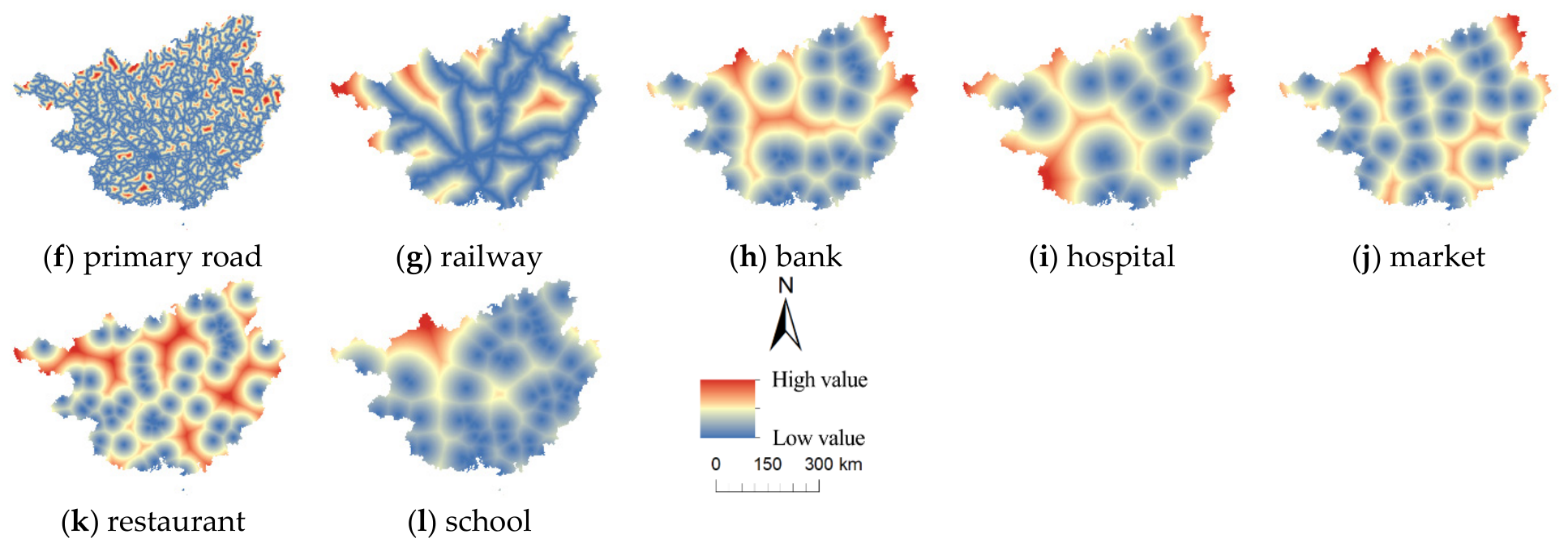
Traffic agent: Based on the regional transportation road network, parcels with higher transportation accessibility tend to exhibit greater expansion potential [35]. The influencing factors for this agent include motorways, primary roads, and railways.

Resident agent: People generally choose to live in areas with well-developed public facilities and moderate population density [36]. The factors influencing this agent include GDP, population, banks, hospitals, markets, restaurants, and schools.

Government agent: Responsible for macro-level regulation. Based on population growth trends and urban green transformation goals, regional redlines for cropland, and construction land are delineated. Simultaneously, DEM and slope data are used to identify ecologically prohibited construction zones.

For the traffic and resident agents, the influence intensity of each factor (except for GDP and population) on a given parcel is quantified as the Euclidean distance from the factor’s location to the centroid of the grid cell. These distance values are then standardized to eliminate dimensional effects. This relationship can be formally expressed as follows [17,29]:

$$\begin{array}{c}{Z}_i^{res}={\beta }_{GDP}{X}_{GDP}+{\beta }_{population}{X}_{population}+{\beta }_{bank}{X}_{bank}+{\beta }_{hospital}{X}_{hospital}+\\ {\beta }_{market}{X}_{market}+{\beta }_{restaurant}{X}_{restaurant}+{\beta }_{school}{X}_{school}\end{array}$$

(12)

$$\begin{array}{c}{Z}_i^{tra}=\end{array}{\beta }_{motorway}{X}_{motorway}+{\beta }_{primary}{X}_{primary}+{\beta }_{railway}{X}_{railway}$$

(13)

$$X_{\alpha }={\displaystyle \frac{1}{\mathit{exp}\left(d_{\alpha }\right)}}$$

(14)

$$\begin{array}{c}{Z}_i^{abm}=Z_i^{res}+Z_i^{tra}+Z_i^{gov}\end{array}$$

(15)

where $Z_i^{res}$, $Z_i^{tra}$ and $Z_i^{gov}$ denote the embedding vectors of the resident, traffic, and government agents, respectively, and $\beta$ represents the influence strength of each social factor. For the government agent, in alignment with the strategic imperatives of “arable land protection” and “ecological priority,” and informed by both the national context of China and the General Land Use Planning of Guangxi, a masking operation is applied to parcels classified as cropland, forest, grassland, and ecologically protected zones. Specifically, parcels within these categories are assigned a binary mask value $M$: $M=1$ indicates that the parcel is prohibited from transitioning to any other land use type, whereas $M=0$ signifies that conversion or retention of the current use is permissible. $Z_i^{abm}$ denotes the fused logits vector.

Finally, the Softmax function is applied to obtain the fused probability $P_{i,C}^{abm}$ for parcel $i$ at time $t$.

2.6. GT-LandSDS

Based on LandSDS, CA serves as the hub that responds to parcel transition probabilities, and the probability of cell $i$ converting to type $s$ at time $t+1$ can be expressed as Equation (16) [19,20].

$$\begin{array}{c}{P}_i^{s,t+1}={\alpha }_1{P}_i^{s,t}+{\alpha }_2{C}_i^t+{\alpha }_3{R}_i^t\end{array}$$

(16)

where $P_i^{s,t}$ denotes the suitability of cell $i$ for transitioning to type $s$ at time $t$; $C_i^t$ represents a mandatory spatial constraint; and $R_i^t$ is a stochastic perturbation term, which can be expressed as $R_i^t=1+{\left(-ln\gamma \right)}^{\alpha }$, where $\gamma$ is a random number uniformly distributed between 0 and 1, and $\alpha$ is an integer parameter ranging from 1 to 10 that controls the intensity of the stochastic disturbance. For computational convenience, this study sets $\alpha =1$. The coefficients ${\alpha }_1$, ${\alpha }_2$, and ${\alpha }_3$ denote the relative weights assigned to the respective components.

For the suitability probability, this study integrates the GAT-derived spatial neighborhood probability $P_i^{gat}$, the transformer-derived temporal sequence probability $P_i^{tf}$, and the ABM-derived agent influence probability $P_i^{abm}$ to obtain the fused suitability probability, as shown in Equation (17).

$$\begin{array}{c}{P}_i^{fused}={\omega }_i^{gat}{P}_i^{gat}+{\omega }_i^{tf}{P}_i^{tf}+{\omega }_i^{abm}{P}_i^{abm}\end{array}$$

(17)

where ${\omega }_i^{gat}$, ${\omega }_i^{tf}$, and ${\omega }_i^{abm}$ denote the learned probability-weighting coefficients for the GAT, transformer, and ABM modules, respectively.

In summary, the transition probability of cell $i$ at time $t$ can be formally expressed by the composite Equation (18) [20].

$$\begin{array}{c}{P}_i^t=a_1{P}_i^{fused}+a_2{\displaystyle \prod _{p=1}^q}C{E}_i^t+a_3{\displaystyle \prod _{u=1}^v}C{P}_i^t+a_4{R}_i^t\end{array}$$

(18)

where ${\prod }_{p=1}^{q}C{E}_{i,p}^t$ represents the mandatory constraints arising from natural environmental factors, and $C{E}_{i,p}^t$ is a binary variable; $C{E}_{i,p}^t=0$ indicates that parcel $i$ is mandatorily constrained by the $p$-th natural environmental factor at time $t$, making it incapable of being converted into or out of its current type, whereas $C{E}_{i,p}^t=1$ indicates otherwise. Here, $q$ denotes the total number of mandatory natural constraints. ${\prod }_{u=1}^{v}C{P}_{i,u}^t$ represents the mandatory constraints arising from national policies, and $C{P}_{i,u}^t$ is a binary variable; $C{P}_{i,u}^t=0$ indicates that parcel $i$ is mandatorily constrained by the $u$-th national policy at time $t$, making it incapable of being converted into or out of its current type, whereas $C{P}_{i,u}^t=1$ indicates otherwise. Here, $v$ denotes the total number of mandatory policy constraints. $a_1$, $a_2$, $a_3$, and $a_4$ represent the weights of the corresponding factors. Following the established practice in Liu et al. (2017), we set $a_1=a_2=a_3=a_4=1$ for computational tractability [17].

3. Study Area and Data

Guangxi is located in southern China within the subtropical monsoon climate zone and is characterized by warm, humid conditions and rich biodiversity. It borders the Beibu Gulf to the south and Vietnam to the southwest, and is the only coastal ethnic autonomous region in China. The region covers approximately 237,600 km² and features higher terrain in the northwest and lower terrain in the southeast with mountains, hills, and plains across the landscape. Karst landforms are well developed, with karst areas accounting for about 37.8% of the total area, making it a typical karst region in China and worldwide.

Karst areas are ecologically fragile, with thin soils, severe soil erosion, and limited vegetation restoration capacity; therefore, land use change has a particularly significant impact on ecosystems [37,38]. In recent years, with the deepening implementation of the Western Development Strategy and the construction of the China–ASEAN Free Trade Area [39,40], Guangxi has experienced rapid socioeconomic development and accelerated urbanization. The demand for construction land has continued to increase, while pressures on cropland conservation and ecological protection have become increasingly prominent [41]. Meanwhile, the promulgation of national policies promoting green transformation has imposed higher requirements on the land use structure and carbon sink functions of karst areas [1,42].

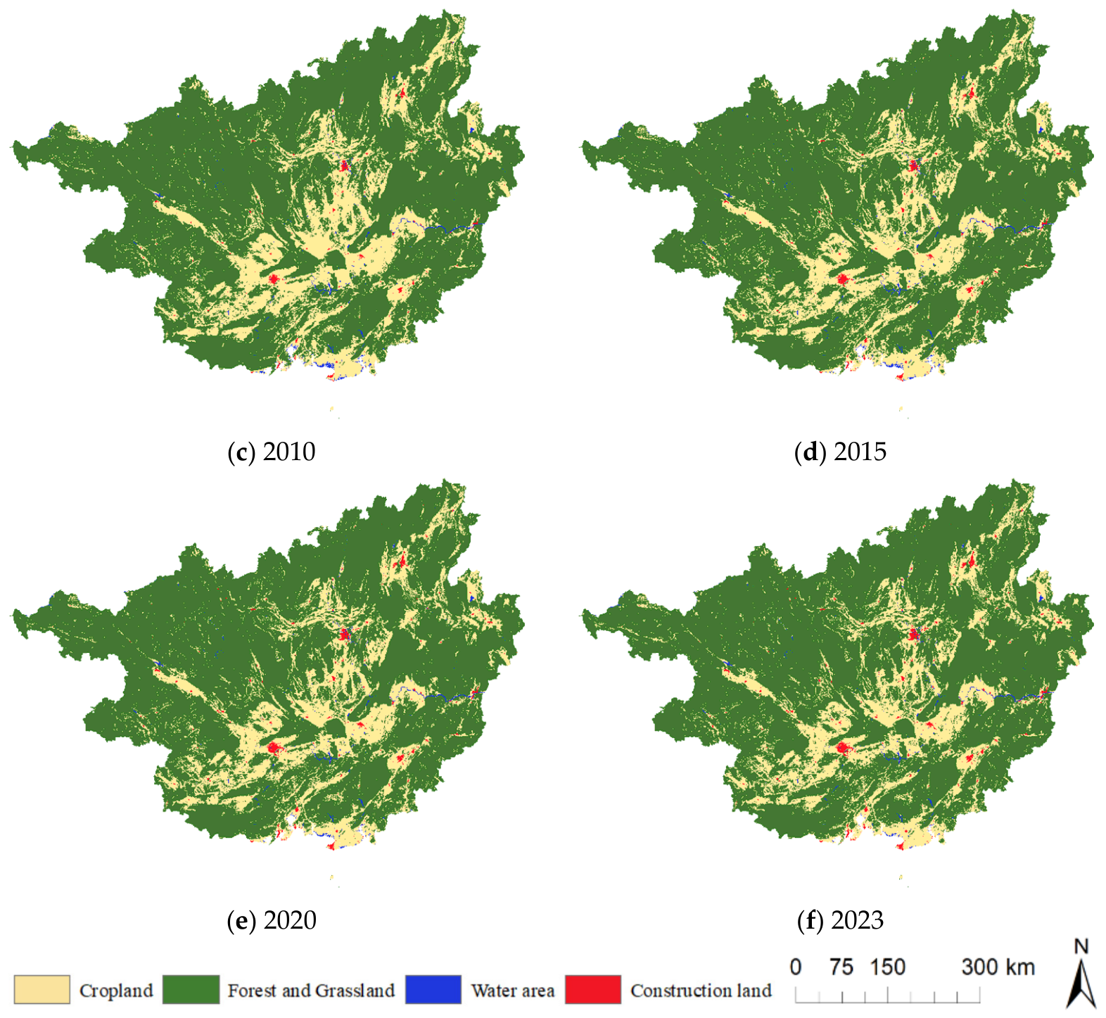
The land use data used in this study were derived from the China Land Cover Dataset (https://irsip.whu.edu.cn (accessed on 26 January 2026)), developed by Yang and Huang (2021) at the Remote Sensing Information Processing Institute at Wuhan University [43]. The dataset was generated on the Google Earth Engine (GEE) platform by integrating multi-temporal Landsat imagery (Landsat 5 TM, 7 ETM+, and 8 OLI) with a Random Forest classifier and spatiotemporal logical post-processing to ensure temporal consistency. The original product has a spatial resolution of 30 m and an overall accuracy exceeding 79.31%. For this study, we extracted LULC maps for six epochs: 2000, 2005, 2010, 2015, 2020, and 2023. To focus on competition and transition among cropland, ecological land, and built-up land, we aggregated forest and grassland into a single ecological land class based on functional homogeneity. The original classification system was then reclassified into four primary categories: cropland, forest and grassland, water area, and construction land, following the standard issued by the Chinese Academy of Sciences. This reclassification was adopted because Guangxi is a subtropical karst mountainous region with a highly fragmented land surface, where the mixed-pixel problem in remote sensing imagery makes it difficult to consistently distinguish the traditional six land use categories. Therefore, the original classes were merged into four broader categories to reduce classification confusion and improve result reliability.

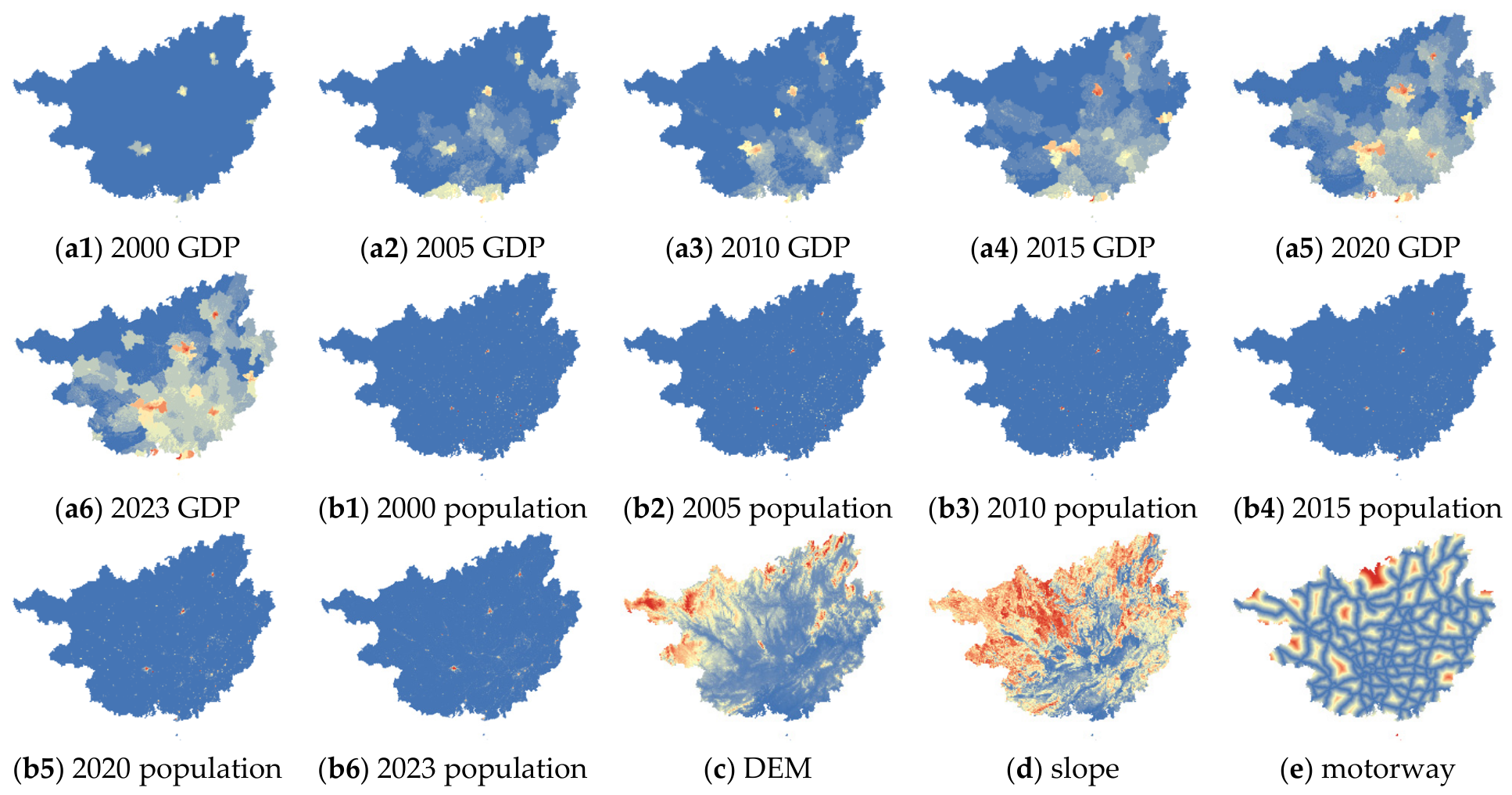
A hierarchical indicator system for natural, social, and economic driving factors was constructed to characterize their spatial and temporal impacts on land use change. Natural environmental data include the digital elevation model (DEM) and slope data for the entire Guangxi. The DEM data were obtained from SRTM1 V3, and the slope data were derived from the DEM.

Socioeconomic driving factors include: (1) China’s population spatial distribution at the kilometer grid level, sourced from the Resource and Environment Science and Data Center (RESDC) (http://www.resdc.cn (accessed on 30 January 2026)) (DOI:10.12078/2017121101) [44]; (2) China GDP spatial distribution at the kilometer grid level, also sourced from RESDC (DOI:10.12078/2017121102) [45], and both GDP and population datasets are spatially and temporally collocated with the six-period land use data; (3) 14 types of infrastructure vector features covering the entire Guangxi, including 4 types of transportation roads (e.g., motorway) and 10 types of public facilities (e.g., park, school), sourced from OpenStreetMap (OSM). To examine the associations between the 14 candidate factors and urban expansion, transition samples of urban expansion were constructed based on construction land parcels. The 14 vector factors were transformed into Euclidean distance variables and screened using univariate logistic regression, variance inflation factor (VIF) diagnostics, and random forest permutation importance. Detailed screening results for all candidate factors are provided in Appendix Table A1. Based on these combined criteria, eight socioeconomic driving factors were retained.

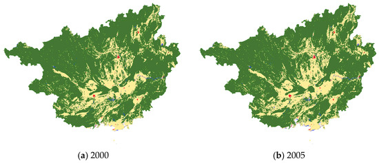
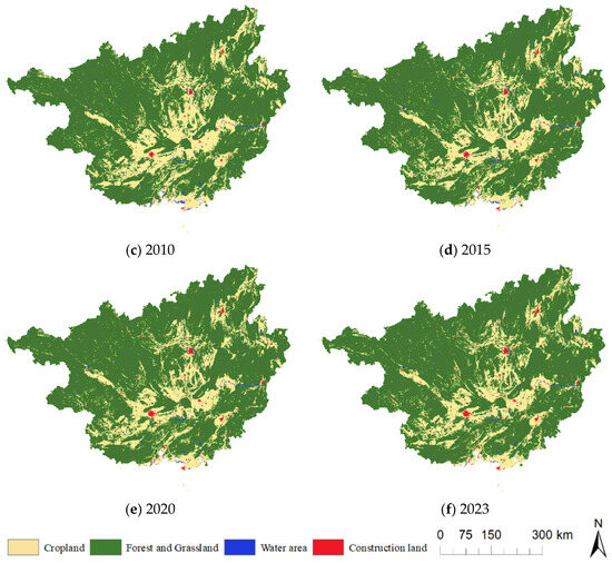
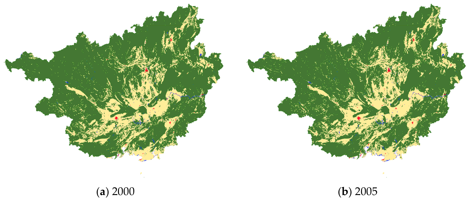
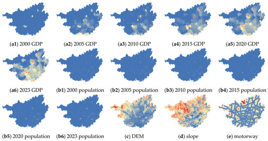
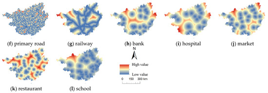
GAT typically requires coupling with VCA and relies on vector parcel data. However, due to data confidentiality and related restrictions, cadastral parcel data for the study area were unavailable. In this study, graph construction follows the object-based and topological neighborhood concept of VCA, while the actual CA units are regular 1000 m raster cells. All data were projected to a uniform coordinate system (WGS 1984 UTM Zone 48N) and resampled to a uniform resolution to ensure spatial alignment. The classification and sources of all data are presented in Table 1; the six-period land use data from 2000 to 2023 are shown in Figure 2; and the raster maps of natural and socioeconomic driving factors are shown in Figure 3.

Table 1. Indicator classification and data information.

First-Level Indicator	Second-Level Indicator	Data Source	Year
Land Use Data	2000 land use data	Landsat 5 TM, Landsat 7 ETM+	2000
	2005 land use data	Landsat 5 TM, Landsat 7 ETM+	2005
	2010 land use data	Landsat 5 TM, Landsat 7 ETM+	2010
	2015 land use data	Landsat 8 OLI	2015
	2020 land use data	Landsat 8 OLI	2020
	2023 land use data	Landsat 8 OLI	2023
Natural indicators	DEM	SRTM1 V3	2015
	Slope	SRTM1 V3	2015
Social indicators	Population	Resource and Environment Science and Data Center	2000, 2005, 2010, 2015, 2020, 2023
	GDP	Resource and Environment Science and Data Center	2000, 2005, 2010, 2015, 2020, 2023
	Motorway features	OpenStreetMap	2020
	Primary features	OpenStreetMap	2020
	Railway features	OpenStreetMap	2020
	Hospital features	OpenStreetMap	2020
	Bank features	OpenStreetMap	2020
	Market features	OpenStreetMap	2020
	Restaurant features	OpenStreetMap	2020
	School features	OpenStreetMap	2020

Figure 2. Land use data for Guangxi from 2000 to 2023.

Figure 3. Raster data on natural and socioeconomic drivers in Guangxi, where (e–l) denote the Euclidean distances from the infrastructure to a given parcel.

4. Results

4.1. Accuracy Assessment Framework

To reduce potential overestimation caused by spatial autocorrelation, an additional spatial block-based validation strategy was introduced. The study area was divided into 50 km × 50 km spatial blocks, and all samples within the same block were assigned to a single subset. This ensured that test samples were spatially separated from the other subsets at the block level. Sampling prioritized stratification by land use category in the target year. For categories with insufficient samples for stratified partitioning, random splitting with a fixed random seed was used to preserve the independence of model training, parameter selection, and final evaluation. After training, we evaluated both classification performance and CA simulation fidelity on the held-out test set.

This study constructs a classification accuracy evaluation system based on the confusion matrix, including overall accuracy (OA), the Kappa coefficient, and the figure of merit (FoM) for change-simulation accuracy [46,47,48].

The FoM metric is used to evaluate the model’s ability to identify both the location and the type of land use change, and its formula is as follows [47]:

$$\begin{array}{c}FoM={\displaystyle \frac{b}{a+b+c+d}}\end{array}$$

(19)

where $a$ denotes the number of parcels where actual change occurred but was not simulated by the model; $b$ denotes the number of parcels where actual change occurred and was correctly simulated; $c$ denotes the number of parcels where actual change occurred but was simulated as an incorrect category; and $d$ denotes the number of parcels where no actual change occurred but were incorrectly simulated as change.

4.2. Sequence-Length Sensitivity Analysis

The model used land use data from five periods (2000, 2005, 2010, 2015, and 2020), together with GDP, population, and Euclidean distance data for static factors, to simulate land use change in 2023. In total, 128 spatial blocks were generated, including 90 for training, 18 for validation, and 20 for testing, corresponding to 165,936, 35,724, and 35,577 samples, respectively. To further examine model robustness under spatially independent testing, the trained GT-LandSDS model was re-evaluated using the spatial block-based test subset. The GAT branch used two layers with 4 attention heads and a hidden dimension of 64, and transformer branch also used two encoder layers, 4 heads, and a hidden dimension of 64. Graph adjacency was constructed with a cKDTree-based spatial neighborhood rule, with the distance threshold automatically determined from the 0.95 quantile of 8-nearest-neighbor distances. The model was trained in full-batch mode using Adam with a learning rate of 0.001 and weight decay of 0.0005, and the number of epochs set to 1000. Validation loss served as the monitoring metric, and early stopping was used to halt training automatically when the accuracy failed to improve for 200 successive epochs.

To further assess the temporal learning robustness of GT-LandSDS, a sequence-length sensitivity analysis was conducted using 2, 3, 4, and 5 historical observations, as in Table 2.

Table 2. Sequence-length sensitivity analysis of GT-LandSDS under different historical input lengths.

Input Sequence	Historical Years	OA	Kappa	FoM
2 time steps	2015, 2020	0.920	0.782	0.020
3 time steps	2010, 2015, 2020	0.918	0.789	0.020
4 time steps	2005, 2010, 2015, 2020	0.924	0.802	0.025
5 time steps	2000, 2005, 2010, 2015, 2020	0.926	0.820	0.034

The results indicate that model performance generally improves as the number of historical time steps increases. Compared with the 2-step and 3-step settings, the 4-step and 5-step inputs yield higher OA, Kappa, and FoM values, suggesting that richer temporal information helps GT-LandSDS better capture land use dynamics. However, the improvement from 4 steps to 5 steps is relatively small, implying that the benefit of additional historical observations may gradually saturate. Overall, the analysis shows that GT-LandSDS is sensitive to temporal input length, and that a moderate number of historical observations is sufficient to achieve stable performance.

4.3. Multi-Model Comparison

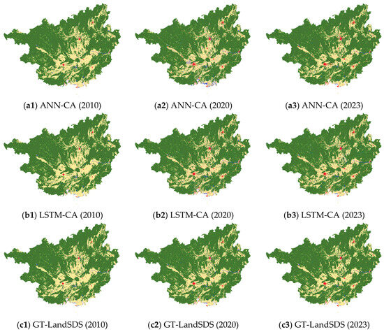
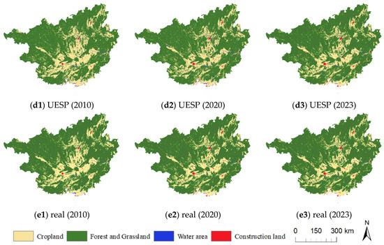
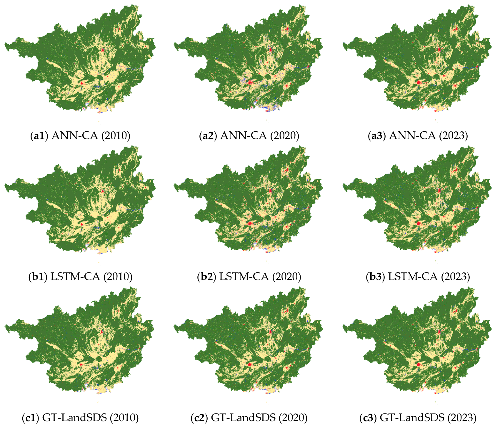
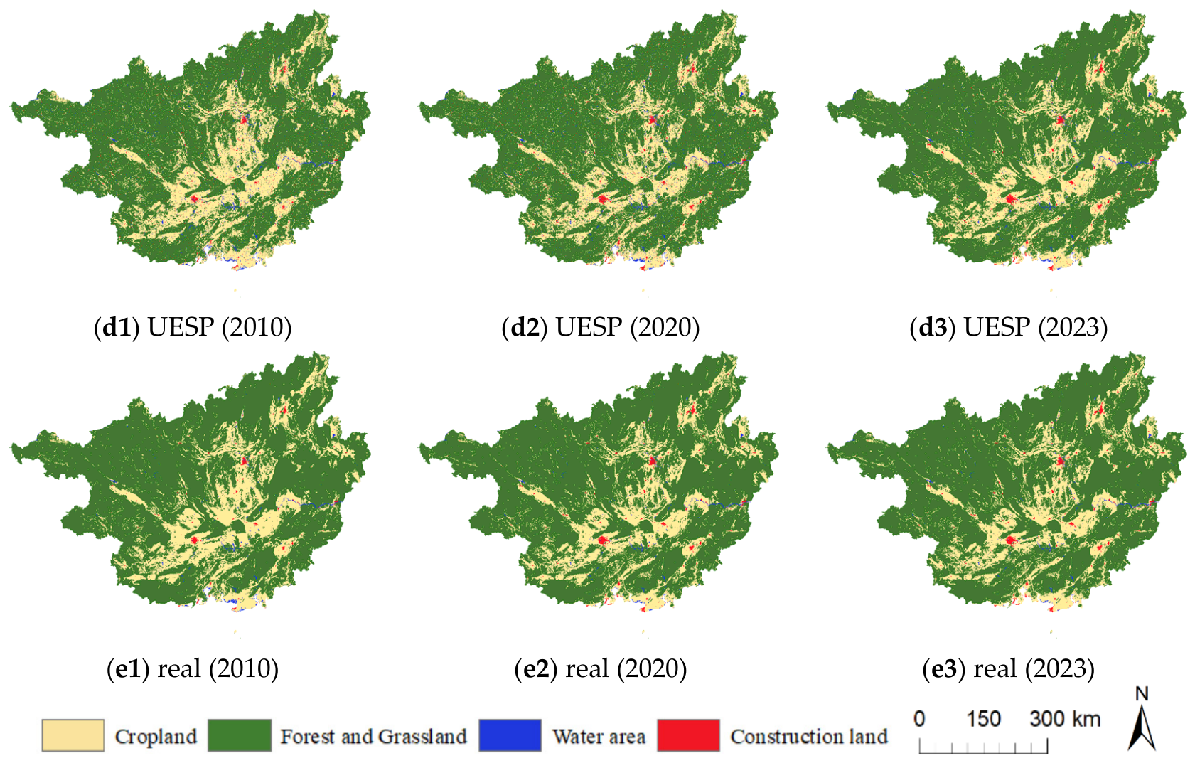
This study employed three additional models, ANN-CA, LSTM-CA, and UESP [29], to simulate land use evolution in Guangxi for 2010, 2020, and 2023. Each model was run ten times under the same data partition and evaluation protocol. Differences between GT-LandSDS and each baseline were tested using Welch’s two-sample t-test (n = 10 repeated runs per model; α = 0.05). For a controlled comparison, all models used the same input data, historical periods, training-validation split, transition constraints, and evaluation settings, with optimization settings kept identical wherever applicable. The simulation results are presented in Figure 4, and the accuracy metrics are listed in Table 3. Owing to the prominent karst landforms in the study area, characterized by fragmented terrain, irregular parcels, and fine-grained patches, the FoM values are generally low. Notably, in the 2010 simulation, GT-LandSDS achieved the highest OA (0.925), while its Kappa (0.832) was slightly lower than that of LSTM-CA (0.836) and UESP (0.840); however, its FoM (0.041) was substantially higher than those of the conventional models. The 2020 simulation followed a similar pattern, with GT-LandSDS obtaining OA/Kappa/FoM values of 0.929/0.826/0.031. The 2023 simulation results further show that GT-LandSDS achieved higher overall metrics than the conventional models, with OA/Kappa/FoM values of 0.926/0.820/0.034. Specifically, OA improved by 3.0% relative to UESP, and FoM increased by 78.9% relative to LSTM-CA. A horizontal comparison within the same model reveals that the FoM values varied across years rather than changing monotonically; GT-LandSDS, ANN-CA, and UESP showed relatively higher FoM in 2010, whereas LSTM-CA achieved its highest FoM in 2023.

Figure 4. Simulation and prediction results for multiple models in 2010, 2020, and 2023.

Table 3. Accuracy evaluation metrics for different models simulating land use in 2010, 2020, and 2023.

Model	Simulation Year	OA (Mean ± SD)	Kappa (Mean ± SD)	FoM (Mean ± SD)
ANN-CA	2010	0.895 ± 0.004	0.816 ± 0.009	0.022 ± 0.005
	2020	0.889 ± 0.003	0.765 ± 0.007	0.010 ± 0.003
	2023	0.875 ± 0.006	0.752 ± 0.011	0.015 ± 0.009
LSTM-CA	2010	0.917 ± 0.003	0.836 ± 0.004	0.016 ± 0.008
	2020	0.925 ± 0.004	0.809 ± 0.009	0.015 ± 0.003
	2023	0.912 ± 0.002	0.801 ± 0.006	0.019 ± 0.006
UESP	2010	0.908 ± 0.003	0.840 ± 0.003	0.035 ± 0.005
	2020	0.915 ± 0.003	0.825 ± 0.007	0.026 ± 0.007
	2023	0.899 ± 0.003	0.821 ± 0.010	0.030 ± 0.005
GT-LandSDS	2010	0.925 ± 0.002	0.832 ± 0.005	0.041 ± 0.005
	2020	0.929 ± 0.003	0.826 ± 0.006	0.031 ± 0.003
	2023	0.926 ± 0.002	0.820 ± 0.003	0.034 ± 0.007

As the results in Appendix Table A2, for the 2023 simulation, GT-LandSDS achieved significantly higher OA than all baselines (p < 0.001) and significantly higher Kappa and FoM than ANN-CA and LSTM-CA (p < 0.001), while its Kappa and FoM were statistically indistinguishable from UESP (p = 0.768 and 0.161). Similar patterns were obtained for 2010 and 2020, with significantly higher OA than all baselines (p < 0.001) and significantly higher FoM than ANN-CA and LSTM-CA (p < 0.001), although its Kappa was significantly lower than that of UESP in 2010 (p < 0.001). These results confirm that the advantage of GT-LandSDS in overall pattern simulation is statistically robust, while its change-reproduction performance remains statistically comparable to UESP.

Overall, multi-temporal information helps improve overall pattern simulation, whereas the low FoM and related change-based metrics indicate that reproducing actual changed areas remains challenging.

To assess the individual roles of the proposed modules, a fixed-checkpoint module suppression analysis was conducted on the 2023 test set (Appendix Table A3 and Table A4). The complete GT-LandSDS model achieved the highest OA (0.937) and Kappa (0.895). Suppressing the direct GAT branch reduced OA to 0.913 and Kappa to 0.766, whereas suppressing the transformer branch reduced OA to 0.911 and Kappa to 0.748. Removing the ABM branch caused smaller decreases in OA and Kappa. Note that the module-suppression metrics in Appendix Table A3 are classification-level: they evaluate the raw fused probabilities before the CA iteration, whereas Table 3 evaluates the end-to-end simulation. This distinction accounts for the higher values in Table A3 and isolates the contribution of each module to the underlying classification, independent of the spatial allocation process. These results indicate that the GAT and transformer branches jointly support the overall classification performance, while ABM provides a supplementary contribution. The higher FoM after suppressing transformer branch further suggests that module effects vary across evaluation metrics.

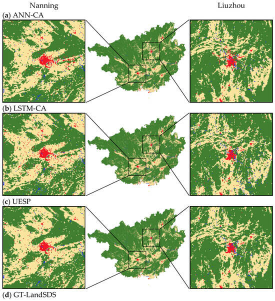
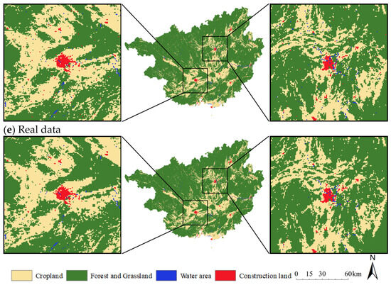
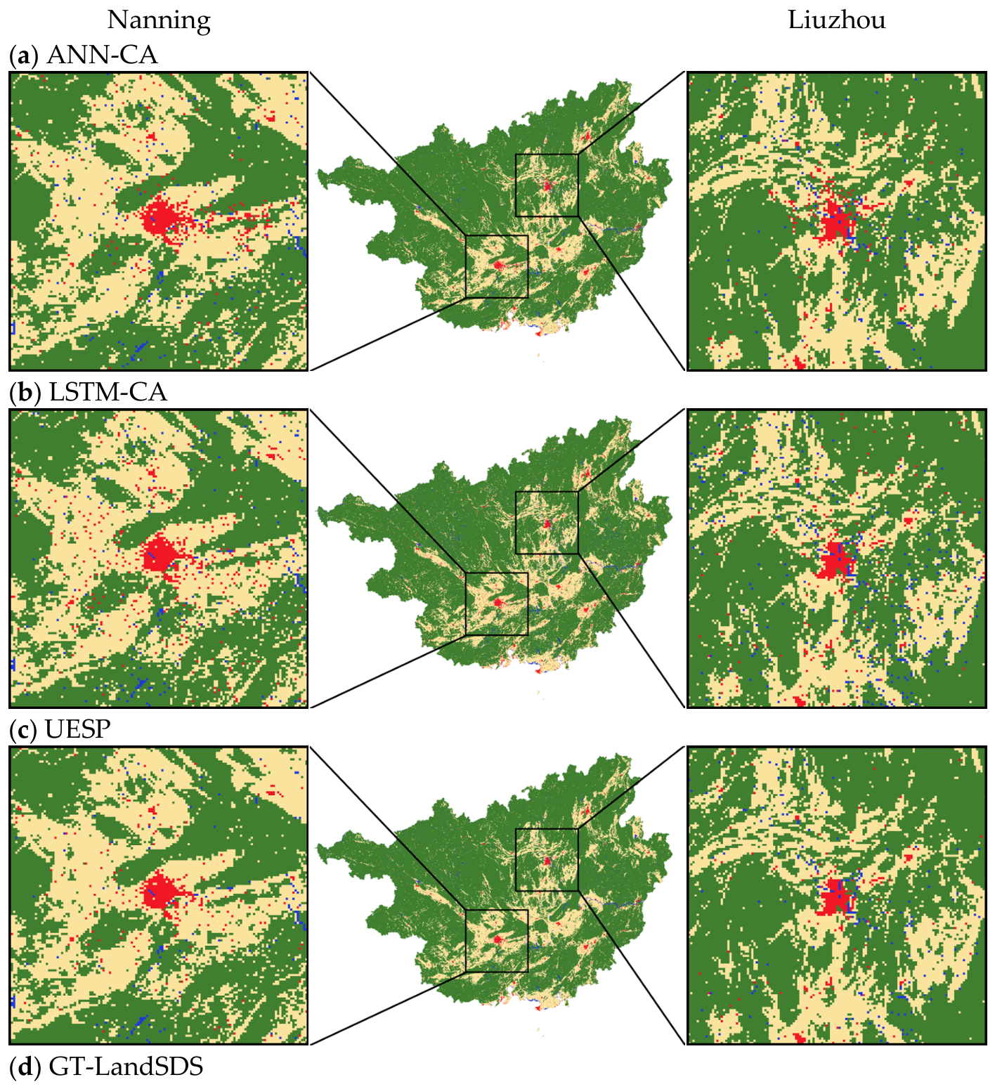
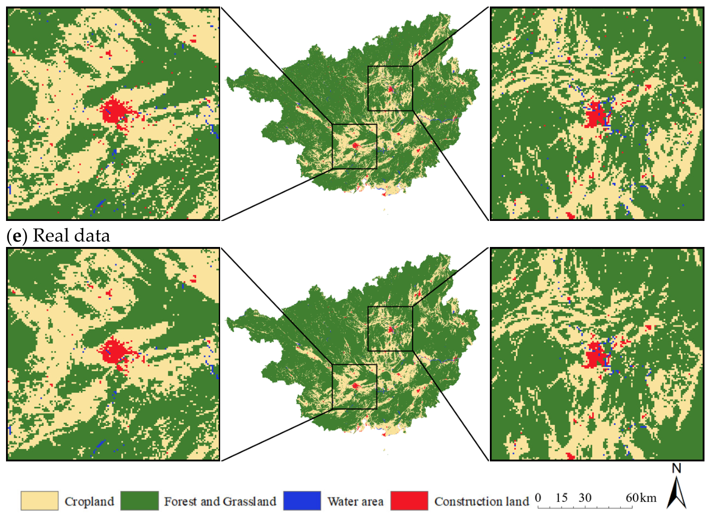
Furthermore, this study selected two rectangular windows centered on Nanning City, the capital and regional gateway of Guangxi, and Liuzhou City, its key industrial city, for a detailed multi-model comparison of urban spatial morphology simulation. The multi-model comparison results are presented in Figure 5.

Figure 5. Details of multi-model simulation results for 2023.

Based on the observed land use change, the expansion of construction land in Nanning in 2023 showed several main directional patterns: southeastward along the Lanhai Expressway, eastward along the Quannan Expressway, southward along the Guang-Kun Expressway, and southwestward along the Shawu and Nanyou expressways. In Liuzhou, construction land expansion in 2023 mainly occurred northeastward along Shuguang Avenue, southeastward along Yanghe Avenue, and southwestward along Liujiang Avenue. According to the simulation results, the ANN-CA model produced scattered construction land growth around the cities, with isolated and dispersed parcels that poorly matched the observed expansion pattern. In contrast, the LSTM-CA, UESP, and GT-LandSDS simulations showed clear directional characteristics, with newly added construction land in Nanning clustered in the eastern, southeastern, and southern areas, and that in Liuzhou distributed along the transportation network, in good agreement with the observed expansion. This indicates that incorporating the temporal dimension helps describe urban expansion morphology. Meanwhile, in the LSTM-CA and UESP results, some newly developed patches remained randomly scattered in areas with low development potential. By contrast, the GT-LandSDS results exhibited a more pronounced clustered pattern, suggesting a relative advantage over other models in representing urban spatial morphology.

5. Future Scenario Simulation

The People’s Government of Guangxi Zhuang Autonomous Region has noted that Guangxi’s urbanization remains in a stage of catching up with and narrowing the gap with the national average. At the same time, as the China–ASEAN Information Harbor, an ASEAN-oriented financial gateway, and the host of the China–ASEAN Expo [41,48], Guangxi has strong strategic demands for the internal and external connectivity of its urban agglomerations and the internal spatial structure of its cities [48]. Furthermore, under the strategic guidance of national policies for green transformation development, Guangxi, as a typical karst ecological barrier and a pioneer area for green development, has been assigned the important role of safeguarding ecological functions and facilitating green transformation. This requires that economic development adhere to the principles of ecological priority and green development, ensuring synergistic progress in socioeconomic advancement and the improvement of ecological environmental quality [41]. Therefore, in view of Guangxi’s strategic positioning and ecological requirements, this study proposes the following scenarios to predict land use conditions in 2035.

Scenario 1: Historical trend continuation. This scenario follows the development trends observed in historical land use data from 2000 to 2023. Based on parcel conversion patterns, water area constraints are applied to rivers and lakes. In contrast, no additional hard constraints—such as policy interventions, ecological protection zones, or cropland redlines—are imposed.

Scenario 2: Theoretical high-intensity urban expansion. This counterfactual scenario is designed as an upper-bound stress test rather than a realistic policy projection. Cropland, forest and grassland, lakes, and other water bodies are left unconstrained so that the model can explore its maximum expansion envelope.

Scenario 3: Karst landform conservation under the green transformation development policy. Based on Guangxi’s territorial spatial planning and the overall goals of Guangxi’s green transformation development [41], this scenario imposes the following constraints.

(1)

By 2035, the forest and grassland coverage rate is projected to be no less than 62.6% (148,510.4 km²).

(2)

By 2035, the urban development boundary shall not exceed 1.3 times the 2023 construction land area (2076.1 km²), thereby setting an upper limit on construction land expansion.

(3)

Land use conversion restrictions apply to 78 ecological protection zones and 145 natural parks throughout Guangxi.

These policy goals were operationalized as quantity constraints, spatial restriction rules, and parcel conversion controls. Quantity constraints defined upper or lower limits for key land use types, spatial restrictions prohibited land conversion within protected or ecologically sensitive areas, and parcel conversion controls adjusted the probability of transitions among land use categories. In this way, abstract policy guidance was converted into spatially explicit and model-operable constraint conditions.

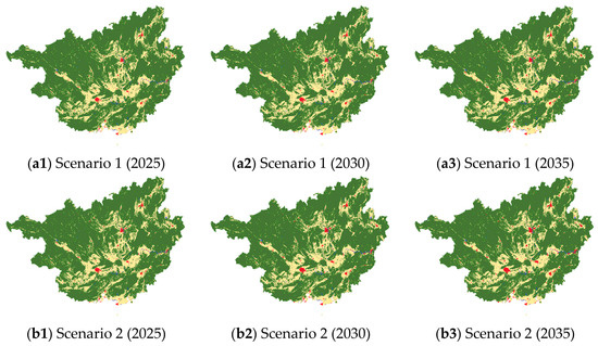
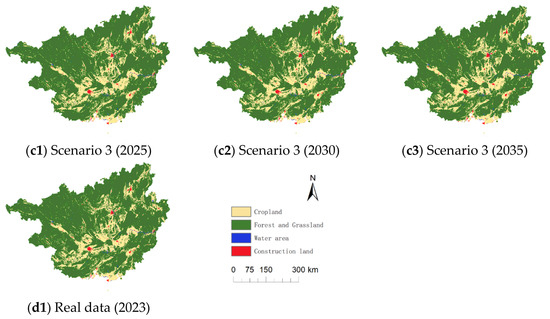
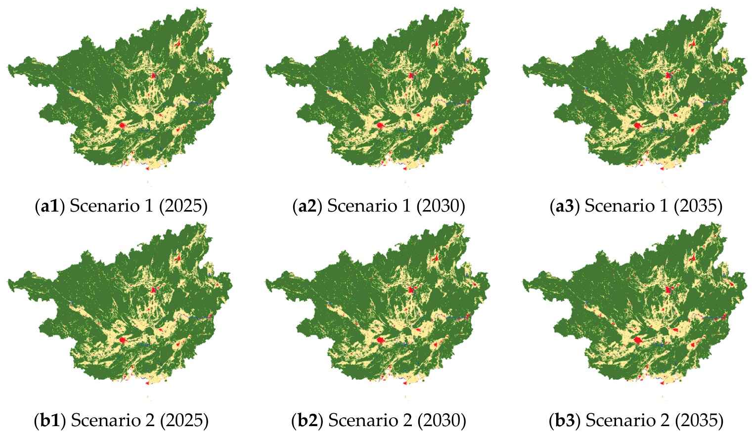
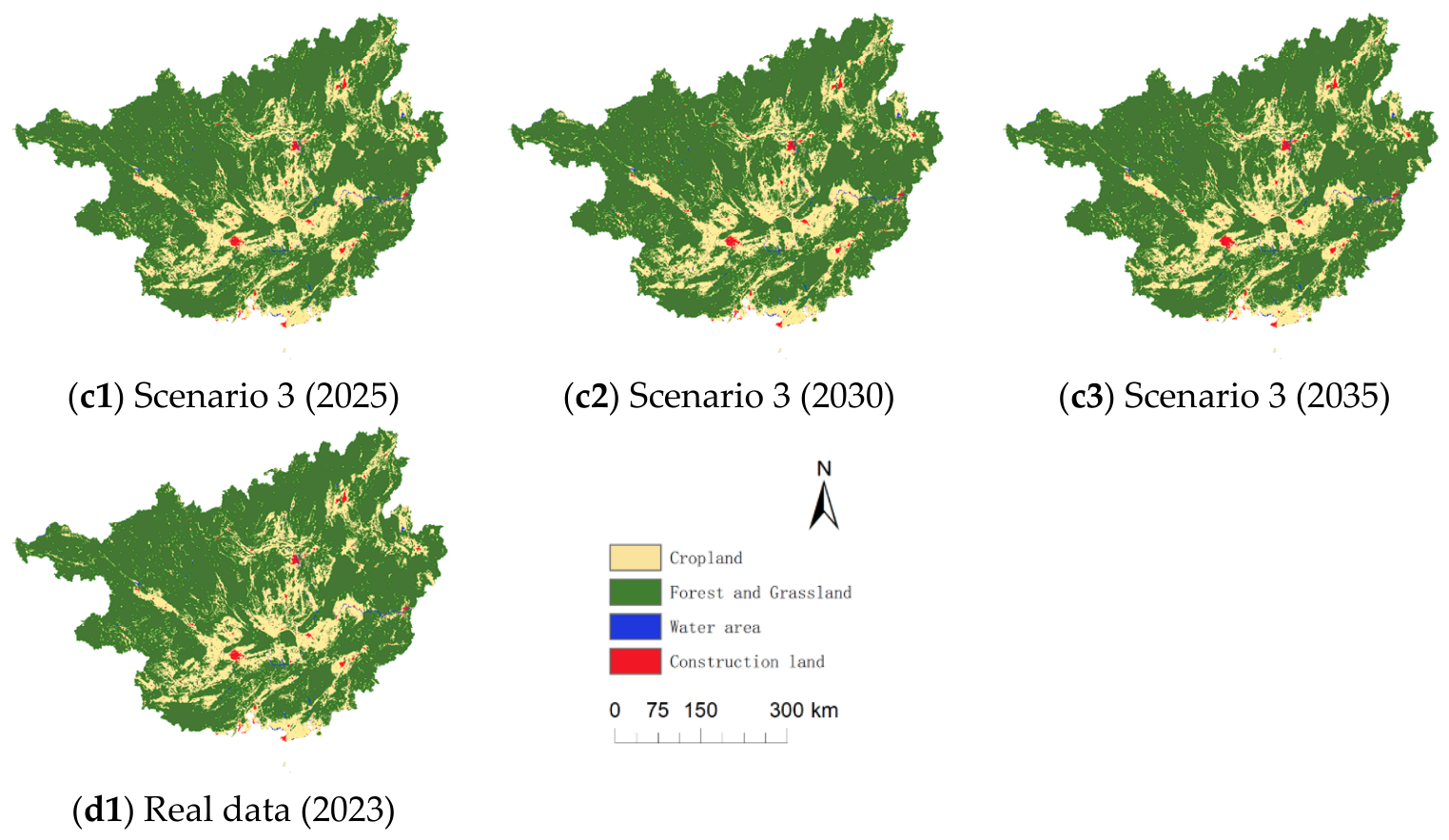
The predicted areas (km²) for each land use type from 2023 to 2035 under the three scenarios are presented in Table 4. The transition matrices for each land use type under the three scenarios are shown in Appendix Table A5, Table A6 and Table A7. The simulation results are shown in Figure 6.

Table 4. Simulation and prediction results for 2025, 2030, and 2035 (km²).

		Cropland	Forest and Grassland	Water Area	Construction Land
real2023		48,272	186,467	901	1597
scenario1	2025	48,028	186,605	911	1693
	2030	47,817	186,553	919	1948
	2035	47,495	186,612	924	2206
scenario2	2025	48,056	186,391	896	1894
	2030	47,660	186,313	887	2377
	2035	47,081	186,268	872	3016
scenario3	2025	48,195	186,513	911	1618
	2030	47,978	186,532	922	1805
	2035	47,782	186,504	930	2021

Figure 6. Simulation and prediction results of different scenarios in 2025, 2030, and 2035.

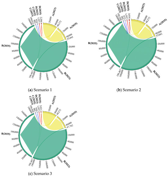
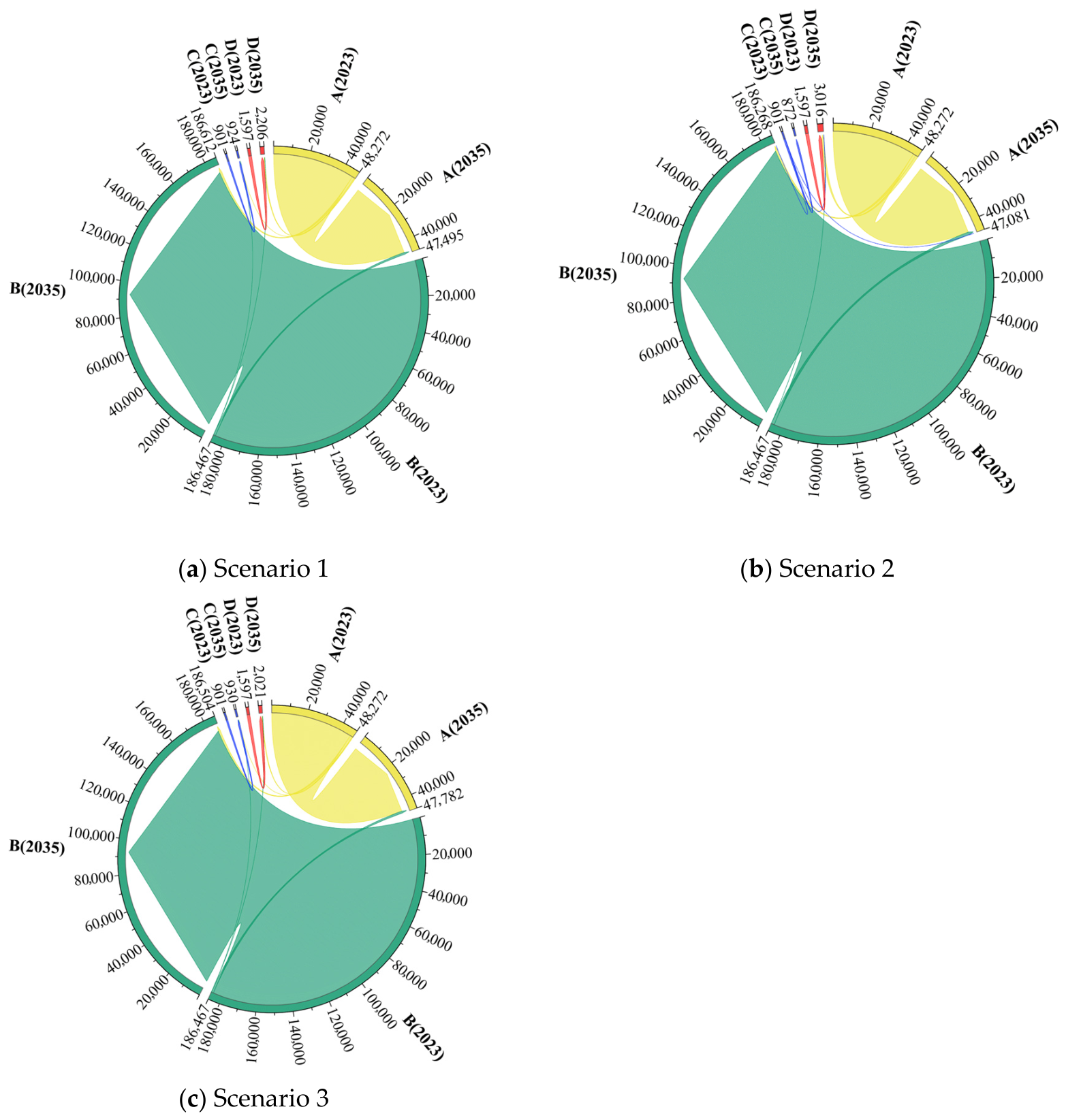
The results reveal significant differences in land use change across scenarios. In Scenario 1 (continuation of historical trends), cropland continued to decrease, while forest and grassland, water areas, and construction land increased. Among them, construction land showed particularly rapid growth, increasing by 38.1% from 2023, while cropland decreased by 1.6%. This indicates that if historical evolution trends persist, urban construction expansion will continue, accompanied by a gradual reduction in cropland. In this scenario, the area changes for each land use type are relatively moderate, and the overall land use transition remains within an acceptable range. The chord diagram of land use type transitions across the three scenarios is shown in Figure 7.

Figure 7. Chord diagram showing land parcel transitions across multi-scenario simulations from 2023 to 2035, where A denotes cropland, B denotes forest and grassland, C denotes water area, D denotes construction land, and (X) denotes the total area of the corresponding land use type in year X.

Scenario 2, aimed at promoting economic development and accelerating urbanization, shows the most dramatic changes. Construction land expanded rapidly from 1597 km² to 3016 km², an increase of 88.9%. Simultaneously, cropland area contracted substantially, declining from 48,272 km² in 2023 to 47,081 km² in 2035, a 2.5% decrease. Water area also decreased slightly, while forest and grassland remained nearly stable. It is evident that if economic development is pursued without restrictions on urban growth, construction land will expand rapidly, mainly at the expense of cropland, thereby intensifying the pressure of urbanization on land resources in Guangxi’s karst region.

Compared with Scenarios 1 and 2, Scenario 3, based on the new urbanization policy, imposes more effective constraints on the growth of construction land. The results show that construction land increased steadily from 2023 to 2035, reaching 2021 km² in 2035, while water areas expanded slowly. Cropland area still declined, but only by 1.0% from 2023 to 2035, which is less than that in Scenarios 1 and 2. Meanwhile, forest and grassland remained relatively stable. This demonstrates that, despite the constraints of the urban development boundary, the forest and grassland redline, and the cropland redline, the disorderly expansion of construction land is effectively controlled, thereby alleviating the loss of cropland and helping to protect the ecological environment of the karst areas.

6. Discussion

6.1. Coupling of the Spatiotemporal Dual-Dimensional Model

This study introduces the GAT-Transformer architecture into the CA framework for the first time and applies it to urban expansion simulation in karst areas. Its main contributions are reflected in three aspects: (1) coupling GAT, which dynamically captures spatial dependencies among parcels, with transformer, which models temporal sequences through the self-attention mechanism, rather than simply combining the two components in a linear manner; (2) integrating the ABM module to embed the decision-making influences of three agent types, namely traffic, resident, and government, into the transition rules, thereby extending the model’s ability to represent micro-level behavioral processes; and (3) providing a feasible framework for integrating static spatial modeling with dynamic temporal modeling in urban expansion simulation. Experimental results indicate that GT-LandSDS has relative advantages in overall accuracy and spatial feature representation, while its change-reproduction ability remains limited.

Compared with existing hybrid models, the GAT-Transformer coupling has two main advantages. First, GAT’s multi-head attention mechanism can dynamically weight the influence of neighboring parcels without relying on predefined neighborhood windows, which is particularly suitable for karst landscapes characterized by fragmented and irregularly distributed parcels. Second, the transformer’s self-attention mechanism makes the relationships among available historical time steps explicit when predicting future states, thereby reducing dependence on strictly sequential memory propagation in recurrent architectures.

6.2. Policy Recommendations Based on Multi-Scenario Simulation Results

Based on the differences observed among the three scenarios, the following policy recommendations are proposed.

First, the annual growth of construction land should be strictly regulated to accommodate urbanization while avoiding excessive occupation of cropland, especially in peri-urban areas where cropland is most vulnerable to expansion pressure. Second, cropland protection should be prioritized in major agricultural production areas and around expanding urban clusters, and permanent basic farmland should be strictly preserved to maintain regional food security. Third, GDP and population growth projections should be incorporated into the dynamic regulation of construction land supply, while a flexible control mechanism linked to cropland protection targets should be established to prevent economic growth from driving disproportionate cropland loss. Fourth, in line with the requirements of territorial spatial planning, the cropland redline, the requisition-compensation balance system, and the annual “in–out balance” mechanism should be strengthened simultaneously, so that urban development, land consolidation, and cropland restoration can be coordinated within a unified governance framework.

6.3. Limitations and Future Directions

Land use change is a complex phenomenon influenced by both natural and social factors across spatial and temporal dimensions.

(1)

The inherent uncertainty of policy interventions and external drivers. In regions of high strategic importance and fragile ecological environments, land use policies are often subject to dynamic adjustment. Rapid changes in ecological redline policies, the redesignation of nature reserves, and the sudden implementation of urban renewal projects can all significantly alter land use trajectories. In addition, this study did not explicitly account for external drivers such as cross-border trade dynamics and ASEAN cooperation, which are increasingly influential in Guangxi’s development. Future research could integrate more diverse data sources, such as cross-border transportation networks and border port development indicators, to refine transition rules and improve the model’s responsiveness to macro-policy shifts.

(2)

The trade-off between temporal resolution and classification noise. This study employed a five-year interval to simulate land use evolution. In ecologically sensitive karst areas, land use conversion is typically a slow-response process; therefore, a six-year timescale can effectively filter out short-term disturbances and capture ecologically meaningful evolutionary patterns. Moreover, annual remote sensing classification data often contain high-frequency noise, which may introduce spurious correlations during deep learning model training. However, this relatively coarse temporal resolution limits the model’s ability to capture abrupt land use changes driven by sudden policy interventions or rapid urbanization at the annual scale. Future studies could adopt finer temporal resolutions to better balance the reduction in classification noise with the capture of high-frequency change signals.

(3)

Uncertainty associated with the classification accuracy of the original land use data. It should be noted that the reclassified land use dataset used in this study has an overall accuracy of 79.31%, which introduces a certain degree of uncertainty into the subsequent analysis. Although this level of accuracy indicates acceptable consistency at the regional scale, potential misclassification among individual land use categories may propagate through the identification of land use transitions and further affect simulation performance. Therefore, the relatively low simulation accuracy may be attributable not only to model limitations but also to uncertainties inherited from the input land use data. Since the focus of this study is regional land use change simulation rather than the evaluation of classification methods, class-specific accuracy assessment is not discussed further here. Future work should incorporate more detailed class-level accuracy analysis and uncertainty quantification to better evaluate error propagation effects. In addition, the land cover maps used in this study are hard categorical products; the adopted China Land Cover Dataset does not provide per-pixel class membership or change probabilities [43]. Classification uncertainty is therefore not propagated into the transition probabilities estimated by GT-LandSDS, and the plausibility of individual transitions is not explicitly modulated by expert knowledge. Future work could exploit multi-temporal membership or change-probability information to quantify, for each parcel, the likelihood that land change has occurred or is occurring. Expert-informed (Bayesian) priors could further modulate the estimated transition probabilities—assigning greater support to plausible conversions such as cropland-to-construction land, and less support to less plausible ones such as cropland-to-forest and grassland or water-to-forest and grassland, thereby complementing, rather than replacing, the data-driven learning process and potentially improving the fidelity of change-based evaluation metrics.

(4)

A further limitation concerns the temporal consistency of the infrastructure driving factors. The infrastructure accessibility variables (motorway, primary road, railway, hospital, bank, market, restaurant, and school) were derived from a single 2020 OpenStreetMap snapshot, whereas the simulations span more than two decades. Although the provincial road network and major public facilities remained largely stable during this period, the motorway network did expand. Ideally, year-by-year infrastructure layers would be used. However, consistent multi-year vector infrastructure data with identical attribute definitions are not publicly available for the study area, which prevents a fully time-varying reconstruction of the accessibility fields. Note that the population and GDP layers are time-varying and were matched to the corresponding land use epochs, whereas DEM and slope are time-invariant. Moreover, the module-suppression analysis (Appendix Table A3) indicates that the socioeconomic and infrastructure component contributes only in a supplementary manner to model performance, suggesting that the temporal inconsistency of these static variables has limited influence on the simulation results. Nevertheless, future work should incorporate time-varying infrastructure data to quantify this effect directly.

6.4. The Constraints Imposed by Spatial Resolution and Computational Complexity

In this study, the research area was partitioned into a 1 km grid, with each cell’s centroid serving as a node, yielding 237,237 nodes. This configuration imposes a significant computational burden, particularly given the quadratic scaling of attention mechanisms in GAT and transformer modules. All models employed in this study, GT-LandSDS, ANN-CA, LSTM-CA, and UESP, were executed on the Colab cloud computing platform (https://colab.research.google.com (accessed on 13 February 2026)) using a Python 3 runtime and an A100 GPU with 80 GB of memory. Detailed runtime and resource information are presented in Table 5. Evidently, the integration of GAT with transformer substantially raises the computational complexity relative to conventional models.

Table 5. Comparison of training time and memory usage across different models.

	First-Epoch Time (s)	Time Per 10 Epochs (s)	CPU Memory Usage (GB)	GPU Memory Usage (GB)
ANN-CA	23.24	0.36	3.7	0.6
LSTM-CA	15.82	3.70	3.7	1.9
UESP	31.68	10.20	3.9	31.0
GT-LandSDS	42.51	13.27	4.0	36.3

Furthermore, in regions with fragmented terrain, such as karst landscapes, a 1 km resolution may overlook subtle changes in smaller, irregular parcels. Therefore, the selection of an appropriate spatial resolution warrants careful consideration and further investigation.

7. Conclusions

Regional land use change simulation requires explicit modeling of complex spatiotemporal dynamics. To address this, this study developed the GT-LandSDS framework, which integrates GAT, transformer, ABM, and CA into a remote sensing-driven simulation model. GAT captures topological dependencies among land parcels and their higher-order neighbors, while transformer models cross-time temporal context from the available multi-period remote sensing observations. By coupling these spatial and temporal representations and incorporating micro-scale human decision-making through ABM, GT-LandSDS supports more detailed simulation of regional land use patterns, while fine-scale change reproduction remains a limitation. The sequence-length sensitivity analysis further suggests that longer historical windows improve temporal robustness, although the gain becomes marginal beyond four steps.

Given Guangxi’s distinctive geographical location and karst geomorphology, balancing economic development with green urban transformation is particularly important. Driven by time-series remote sensing observations, GT-LandSDS was used to simulate land use patterns and transitions in Guangxi for 2010, 2020, and 2023. In the 2023 simulation, the model achieved an overall accuracy of 0.926, a Kappa coefficient of 0.820, and a FoM of 0.034. Compared with conventional models, it showed relative advantages in representing urban spatial morphology, while the low FoM indicates limited capability in reproducing actual changed areas. The sequence-length sensitivity analysis likewise supports the use of multi-period historical inputs, while indicating that change reproduction remains the main limitation.

This study further designed three scenarios for future land use simulation in Guangxi, namely historical trend continuation, theoretical high-intensity urban expansion, and green urban transformation policy. By incorporating strong constraint factors, such as nature reserves, forest and grassland redlines, and urban development boundaries, the model projected land use change and spatial distribution patterns for 2035. The scenario results differed substantially: in Scenario 2, construction land expanded rapidly, whereas in Scenario 3, construction land was more strictly constrained and cropland was better protected. Based on these findings, this study recommends prioritizing the protection of cropland and establishing a flexible land use constraint mechanism.

Overall, the GT-LandSDS framework provides a quantitative reference for understanding the long-term effects of land use policies and supports more informed planning in ecologically fragile karst regions under rapid urbanization.

References

- The Central Committee of the Communist Party of China and the State Council. Opinions on Promoting High-Quality Urban Development; The Central Committee of the Communist Party of China and the State Council: Beijing, China, 2025. [Google Scholar]
- Camagni, R.; Gibelli, M.C.; Rigamonti, P. Urban mobility and urban form: The social and environmental costs of different patterns of urban expansion. Ecol. Econ. 2002, 40, 199–216. [Google Scholar] [CrossRef] [Scilit]
- Zhang, W.C. A Study on the Pattern of Industrial Wave Expanding Along Traffic Economic Belts. Prog. Geogr. 2000, 19, 335–342. [Google Scholar]
- Chaturvedi, V.; de Vries, W.T. Machine Learning Algorithms for Urban Land Use Planning: A Review. Urban Sci. 2021, 5, 68. [Google Scholar] [CrossRef] [Scilit]
- Hasan, S.S.; Zhen, L.; Miah, M.G.; Ahamed, T.; Samie, A. Impact of land use change on ecosystem services: A review. Environ. Dev. 2020, 34, 100527. [Google Scholar] [CrossRef] [Scilit]
- Liu, Y.; Batty, M.; Wang, S.Q.; Corcoran, J. Modelling urban change with cellular automata: Contemporary issues and future research directions. Prog. Hum. Geogr. 2021, 45, 3–24. [Google Scholar] [CrossRef] [Scilit]
- Li, X.C.; Liu, X.P.; Yu, L. A systematic sensitivity analysis of constrained cellular automata model for urban growth simulation based on different transition rules. Int. J. Geogr. Inf. Sci. 2014, 28, 1317–1335. [Google Scholar] [CrossRef] [Scilit]
- Hu, S.; Deren, L. Vector Cellular Automata Based Geographical Entity. In Proceedings of the 12th International Conference on Geoinformatics (Geospatial Information Research), Gävle, Sweden, 7–9 June 2004. [Google Scholar]
- Moreno, N.; Wang, F.; Marceau, D.J. Implementation of a dynamic neighborhood in a land-use vector-based cellular automata model. Comput. Environ. Urban Syst. 2009, 33, 44–54. [Google Scholar] [CrossRef] [Scilit]
- Barreira-González, P.; Gómez-Delgado, M.; Aguilera-Benavente, F. From raster to vector cellular automata models: A new approach to simulate urban growth with the help of graph theory. Comput. Environ. Urban Syst. 2015, 54, 119–131. [Google Scholar] [CrossRef] [Scilit]
- Moreno, N.; Méenard, A.; Marceau, D.J. VecGCA: A vector-based geographic cellular automata model allowing geometric transformations of objects. Environ. Plan. B 2008, 35, 647–665. [Google Scholar] [CrossRef] [Scilit]
- Liu, X.P.; Liang, X.; Li, X.; Xu, X.C.; Ou, J.P.; Chen, Y.M.; Li, S.Y.; Wang, S.J.; Pei, F.S. A future land use simulation model (FLUS) for simulating multiple land use scenarios by coupling human and natural effects. Landsc. Urban Plan. 2017, 168, 94–116. [Google Scholar] [CrossRef] [Scilit]
- Zhang, X.; Chen, P.; Cai, Y.; Lin, J. Prediction of PM2.5 Concentrations in the Pearl River Delta by Integrating the PLUS and LUR Models. Land 2026, 15, 240. [Google Scholar] [CrossRef] [Scilit]
- Feng, Y.; Tong, X. Dynamic land use change simulation using cellular automata with spatially nonstationary transition rules. GISci. Remote Sens. 2018, 55, 678–698. [Google Scholar] [CrossRef] [Scilit]
- Liang, X.; Guan, Q.F.; Clarke, K.C.; Liu, S.S.; Wang, B.Y.; Yao, Y. Understanding the drivers of sustainable land expansion using a patch-generating land use simulation (PLUS) model: A case study in Wuhan, China. Comput. Environ. Urban Syst. 2021, 85, 101569. [Google Scholar] [CrossRef] [Scilit]
- Wu, X.; Liu, X.; Zhang, D.; Zhang, J.; He, J.; Xu, X. Simulating mixed land-use change under multi-label concept by integrating a convolutional neural network and cellular automata: A case study of Huizhou, China. GISci. Remote Sens. 2022, 59, 609–632. [Google Scholar] [CrossRef] [Scilit]
- Liu, D.Y.; Zheng, X.Q.; Zhang, C.X.; Wang, H.B. A new temporal-spatial dynamics method of simulating land-use change. Ecol. Model. 2017, 350, 1–10. [Google Scholar] [CrossRef] [Scilit]
- Liu, D.Y.; Zheng, X.Q.; Wang, H.B.; Zhang, C.X.; Li, J.Y.; Lv, Y.Q. Interoperable scenario simulation of land-use policy for Beijing-Tianjin-Hebei region, China. Land Use Policy 2018, 75, 155–165. [Google Scholar] [CrossRef] [Scilit]
- Liu, D.Y.; Zheng, X.Q.; Wang, H.B. Land-use Simulation and Decision-Support system (LandSDS): Seamlessly integrating system dynamics, agent-based model, and cellular automata. Ecol. Model. 2020, 417, 108924. [Google Scholar] [CrossRef] [Scilit]
- Liu, D.Y. Construction and Application Research of Temporal-Spatial Dynamics Model; Geological Publishing House: Beijing, China, 2024. [Google Scholar]
- Zhai, Y.; Yao, Y.; Guan, Q.; Liang, X.; Li, X.; Pan, Y.; Yue, H.; Yuan, Z.; Zhou, J. Simulating urban land use change by integrating a convolutional neural network with vector-based cellular automata. Int. J. Geogr. Inf. Sci. 2020, 34, 1475–1499. [Google Scholar] [CrossRef] [Scilit]
- Xing, W.; Qian, Y.; Guan, X.; Yang, T.; Wu, H. A novel cellular automata model integrated with deep learning for dynamic spatio-temporal land use change simulation. Comput. Geosci. 2020, 137, 104430. [Google Scholar] [CrossRef] [Scilit]
- Gharaibeh, A.; Shaamala, A.; Obeidat, R.; Al-Kofahi, S. Improving land-use change modeling by integrating ANN with Cellular Automata-Markov Chain model. Heliyon 2020, 6, e05092. [Google Scholar] [CrossRef] [Scilit]
- Wu, Z.; Pan, S.; Chen, F.; Long, G.; Zhang, C.; Yu, P.S. A Comprehensive Survey on Graph Neural Networks. IEEE Trans. Neural Netw. Learn. Syst. 2021, 32, 4–24. [Google Scholar] [CrossRef] [Scilit]
- Vrahatis, A.G.; Lazaros, K.; Kotsiantis, S. Graph Attention Networks: A Comprehensive Review of Methods and Applications. Future Internet 2024, 16, 318. [Google Scholar] [CrossRef] [Scilit]
- Velickovic, P.; Cucurull, G.; Casanova, A.; Romero, A.; Liò, P.; Bengio, Y. Graph Attention Networks. arXiv 2017, arXiv:1710.10903. [Google Scholar]
- Guan, X.F.; Xing, W.R.; Li, J.B.; Wu, H.Y. HGAT-VCA: Integrating high-order graph attention network with vector cellular automata for urban growth simulation. Comput. Environ. Urban Syst. 2023, 99, 101900. [Google Scholar] [CrossRef] [Scilit]
- Guan, Q.F.; Li, J.F.; Zhai, Y.Q.; Liang, X.; Yao, Y. HashGAT-VCA: A vector cellular automata model with hash function and graph attention network for urban land-use change simulation. Landsc. Urban Plan. 2024, 250, 105145. [Google Scholar] [CrossRef] [Scilit]
- Gao, Y.Q.; Liu, D.Y.; Zheng, X.Q.; Wang, X.L.; Ai, G. Urban Expansion Scenario Prediction Model: Combining Multi-Source Big Data, a Graph Attention Network, a Vector Cellular Automata, and an Agent-Based Model. Remote Sens. 2025, 17, 2272. [Google Scholar] [CrossRef] [Scilit]
- Chen, X.; Guan, X.; Xu, Q.; Jiang, L.; Wu, H. UniGCA: A universal graph cellular automata framework for both raster- and vector-based urban growth simulation. Int. J. Digit. Earth 2026, 19, 2672204. [Google Scholar] [CrossRef] [Scilit]
- Liu, X.; Andersson, C. Assessing the impact of temporal dynamics on land-use change modeling. Comput. Environ. Urban Syst. 2004, 28, 107–124. [Google Scholar] [CrossRef] [Scilit]
- Zhou, Y.; Huang, C.; Wu, T.; Zhang, M.Y. A novel spatio-temporal cellular automata model coupling partitioning with CNN-LSTM to urban land change simulation. Ecol. Model. 2023, 482, 110394. [Google Scholar] [CrossRef] [Scilit]
- Yao, Y.; Zhou, K.; Liu, C.X.; Sun, Z.H.; Chen, D.S.; Li, L.L.; Cheng, T.; Guan, Q.F. Temporal-VCA: Simulating urban land use change using coupled temporal data and vector cellular automata. Cities 2024, 149, 104975. [Google Scholar] [CrossRef] [Scilit]
- Vaswani, A.; Shazeer, N.; Parmar, N.; Uszkoreit, J.; Jones, L.; Gomez, A.N.; Kaiser, L.; Polosukhin, I. Attention is All you Need. In Proceedings of the Neural Information Processing Systems, Long Beach, CA, USA, 4–9 December 2017. [Google Scholar]
- Li, L.N.; Huang, C.C.; Liu, Y.S. Detecting the contribution of transport development to urban construction land expansion in the Beijing-Tianjin-Hebei region of China based on machine learning. Land Use Policy 2025, 157, 107622. [Google Scholar] [CrossRef] [Scilit]
- Roback, J. Wages, Rents, and the Quality of Life. J. Political Econ. 1982, 90, 1257–1278. [Google Scholar] [CrossRef] [Scilit]
- D’Ettorre, U.S.; Liso, I.S.; Parise, M. Desertification in karst areas: A review. Earth-Sci. Rev. 2024, 253, 104786. [Google Scholar] [CrossRef] [Scilit]
- Luo, Q.; Zhao, C.W.; Bai, X.Y. The Response of Ecosystem Services to the Intensity of Human Activities and Their Constraint Effects in the Karst Region of Southwest China. Earth Environ. 2026, 54, 193–204. [Google Scholar] [CrossRef] [Scilit]
- The Central Committee of the Communist Party of China and the State Council. Guiding Opinions on Promoting the Development of the Western Region in the New Era to Form a New Pattern; The Central Committee of the Communist Party of China and the State Council: Beijing, China, 2020. [Google Scholar]
- Wu, Z.L.; Zhao, J.Y.; Fu, L.N. The Evolution and Prospect of the Western Development Strategy. In Annual Report on Economic Development in Western Region of China (2025); Wu, Z.L., Ed.; Social Sciences Academic Press: Beijing, China, 2025; pp. 1–50. [Google Scholar]
- People’s Government of Guangxi Zhuang Autonomous Region. The Outline of the Fifteenth Five-Year Plan for National Economic and Social Development of Guangxi Zhuang Autonomous Region; People’s Government of Guangxi Zhuang Autonomous Region: Nanning, China, 2026. [Google Scholar]
- Lin, J.; Li, J.; Rao, Z.; Zeng, Y. Association Between Morphological Spatial Patterns of Built-Up Land and Carbon Emissions: Evidence from 303 Cities in China. Systems 2026, 14, 595. [Google Scholar] [CrossRef] [Scilit]
- Yang, J.; Huang, X. The 30 m annual land cover dataset and its dynamics in China from 1990 to 2019. Earth Syst. Sci. Data 2021, 13, 3907–3925. [Google Scholar] [CrossRef] [Scilit]
- Xu, X.L. 1 km Grid Population Dataset of China; Data Center for Resources and Environmental Sciences, Chinese Academy of Sciences (RESDC): Beijing, China, 2017. [Google Scholar] [CrossRef]
- Xu, X.L. 1 km Grid GDP Dataset of China; Data Center for Resources and Environmental Sciences, Chinese Academy of Sciences (RESDC): Beijing, China, 2017. [Google Scholar] [CrossRef]
- Congalton, R.G. A Review of Assessing the Accuracy of Classifications of Remotely Sensed Data. Remote Sens. Environ. 1991, 37, 35–46. [Google Scholar] [CrossRef] [Scilit]
- Pontius, R.G.; Boersma, W.; Castella, J.C.; Clarke, K.; de Nijs, T.; Dietzel, C.; Duan, Z.; Fotsing, E.; Goldstein, N.; Kok, K.; et al. Comparing the input, output, and validation maps for several models of land change. Ann. Reg. Sci. 2008, 42, 11–37. [Google Scholar] [CrossRef] [Scilit]
- People’s Government of Guangxi Zhuang Autonomous Region. Guangxi New Urbanization Plan (2021–2035); People’s Government of Guangxi Zhuang Autonomous Region: Nanning, China, 2021. [Google Scholar]
Disclaimer/Publisher’s Note: The statements, opinions and data contained in all publications are solely those of the individual author(s) and contributor(s) and not of MDPI and/or the editor(s). MDPI and/or the editor(s) disclaim responsibility for any injury to people or property resulting from any ideas, methods, instructions or products referred to in the content. |
© 2026 by the authors. Licensee MDPI, Basel, Switzerland. This article is an open access article distributed under the terms and conditions of the Creative Commons Attribution (CC BY) license.