Estimating Annual Wildfire-Related Potential Above-Ground Biomass Loss in Eastern Canadian Boreal Forests Using Multi-Source Remote Sensing and XGBoost

Highlights

What are the main findings?

• Integrating optical, L-band SAR, environmental, and geographic predictors provides the most accurate above-ground biomass estimates.
• Wildfires potentially affected 269.20 Mt of above-ground biomass between 2018 and 2024, with 76.7% of the total occurring in 2023.

What are the implications of the main findings?

• Multi-source data integration improves the robustness of large-area biomass mapping in eastern Canadian boreal forests.
• The developed framework supports spatially explicit assessments of wildfire-related biomass impacts and forest carbon dynamics.

Abstract

Wildfire impact assessment requires information on both burned areas and the biomass exposed within burned landscapes. We developed a field-calibrated, multi-source remote-sensing framework to estimate above-ground biomass (AGB) and quantify annual wildfire-related potential AGB exposure across the boreal forests of Quebec and Ontario, Canada, during 2018–2024. The dataset comprised 3725 plot-year AGB observations linked to optical, Sentinel-1 C-band, ALOS L-band synthetic aperture radar, environmental, and geographic predictors. Product-wise screening reduced the 91 candidate predictors to 28. An optimized extreme gradient boosting (XGBoost) model was evaluated using five-fold grouped cross-validation, with repeated observations from each plot assigned to a single fold. The model achieved an RMSE of 25.08 ± 0.36 t ha⁻¹, an MAE of 20.89 ± 0.39 t ha⁻¹, and an R² of 0.53 ± 0.02. The full multi-source configuration outperformed all reduced-source and source-only configurations, while removing ALOS L-band SAR or environmental/geographic predictors produced among the largest performance declines. The model was applied to 9937 land-cover-stratified points within wildfire polygons using predictors from the year preceding each fire. Under the complete-loss assumption, cumulative potential AGB exposure was 269.20 Mt across 6.66 Mha of effective burned area, with a 95% bootstrap interval of 254.19–284.06 Mt reflecting finite-point sampling uncertainty and an area-weighted mean exposure intensity of 40.43 t ha⁻¹. The 2023 fire season accounted for 206.44 Mt, representing 76.7% of cumulative exposure and 73.2% of effective burned area. Effective burned area and total potential exposure were strongly correlated (r = 0.99), whereas exposure intensity followed a distinct pattern and peaked in 2022 at 46.86 t ha⁻¹. Thus, burned area was the primary correlate of regional potential biomass exposure, whereas exposure intensity reflected variation in pre-fire biomass among burned landscapes. These estimates represent potential exposure rather than measured combustion, mortality, or carbon emissions and demonstrate the value of integrating spatially explicit pre-fire AGB with wildfire perimeters.

1. Introduction

Boreal forests constitute a major global forest biome and play important roles in carbon storage, biodiversity conservation, climate regulation, and ecosystem functioning [1,2,3]. Above-ground biomass (AGB) is a key indicator of these functions because it reflects forest structure, productivity, carbon storage, and response to disturbance. Spatially explicit AGB estimates are therefore important for carbon accounting, forest monitoring, ecological modeling, and management, particularly in regions where forest composition and disturbance regimes are changing rapidly [4,5,6,7].

Wildfire is a dominant stand-replacing disturbance in Canadian boreal forests and can rapidly alter biomass stocks, successional trajectories, and regional carbon balance [8,9]. The exceptional 2023 Canadian fire season illustrated the scale of these effects through extensive burning in Quebec and unusually high national fire-related carbon emissions [9,10]. Recent optical and multisensor approaches have improved burned-area delineation [11,12], whereas Sentinel-1 SAR time-series methods support continuous monitoring and identification of the timing of fire-induced forest loss [13]. Yet, the burned area does not indicate how much biomass was present within the affected landscape. Actual biomass consumption and post-fire structural change depend on pre-fire biomass, burn severity, combustion completeness, and residual vegetation [14,15,16]; consequently, fires of similar size may affect markedly different amounts of biomass. We therefore distinguish total potential AGB exposure from exposure intensity, which is defined here as potential AGB exposure per unit of effective burned area (t ha⁻¹). This distinction separates the influence of fire extent from spatial variation in pre-fire biomass density. In this study, potential AGB loss refers to the estimated pre-fire AGB within mapped burned areas under a complete-loss assumption and therefore represents potential biomass exposure rather than directly measured biomass consumption, mortality, combustion completeness, or carbon emissions.

Estimating biomass exposure over large regions requires spatially continuous AGB information. Field inventories provide the empirical basis for biomass estimation, but their spatial coverage is limited. Remote sensing extends these observations by capturing complementary aspects of forest canopies and site conditions. Optical data describe canopy greenness, red-edge response, moisture, and disturbance-related spectral variation, although spectral saturation can reduce sensitivity in high-biomass forests [17,18,19,20]. C- and L-band SAR observations add sensitivity to canopy structure, woody components, and moisture-dependent scattering [21,22,23]. Light detection and ranging (LiDAR) observations further constrain canopy height and vertical structure, which passive optical data do not directly represent [24,25,26]. Environmental and geographic variables can represent broader controls related to climate, topography, soils, productivity, and disturbance history, particularly in heterogeneous boreal landscapes [4,5,27].

Multi-source integration is increasingly used to mitigate the limitations of individual sensors and improve AGB mapping across structurally diverse forests [5,22,28,29,30]. Machine-learning methods are well suited to this task because they can represent nonlinear relationships and interactions between AGB and heterogeneous spectral, radar, structural, and environmental predictors [26,31,32,33,34]. Predictive performance, however, depends not only on algorithm choice but also on predictor composition and redundancy, as highly correlated or weakly informative variables may add noise without providing substantial independent information [21,35]. Feature-selection procedures can address this problem by retaining informative variables and producing more parsimonious models, although their effects on accuracy vary among ecosystems, biomass ranges, and sensor configurations [18,21,34,35,36]. Model evaluation is also sensitive to the characteristics, spatial distribution, and representativeness of the reference observations, as well as to the validation design. These differences should be considered when comparing reported accuracies among studies conducted in different regions or using different reference datasets and validation strategies [4,29].

Recent remote-sensing studies of above-ground biomass (AGB) have largely focused on mapping standing biomass stocks and evaluating whether the integration of optical, synthetic aperture radar (SAR), LiDAR, environmental data, and machine-learning algorithms improves predictive accuracy [5,21,22,23,29]. A complementary body of research has linked forest-disturbance observations to existing biomass products. In Canada, national-scale products have spatialized forest attributes, including AGB, using inventory information and dense Landsat time series [4], and have combined Landsat–Sentinel-2 disturbance detection with spatial biomass products to characterize intra- and interannual AGB dynamics [7]. For the exceptional 2023 Canadian fire season, medium-resolution change detection was used to refine burned-area estimates and quantify the treed AGB affected by fire [9], whereas satellite-constrained atmospheric inversions quantified associated fire-carbon emissions [10]. Event-based studies outside Canada have also used pre- and post-fire LiDAR and multisensor imagery to estimate fire-induced structural change, biomass consumption, or carbon emissions. Collectively, these studies demonstrate that mapped fire extent alone does not determine biomass impacts: pre-fire forest structure, spatial variation in fuel stocks, burn severity, and assumed biomass-loss or combustion fractions also influence the resulting estimates [14,15,16].

Despite these advances, a field-calibrated and multi-year framework that consistently links predicted pre-fire AGB to annual wildfire polygons remains lacking for the boreal forests of Quebec and Ontario. Existing Canadian studies have generally emphasized national forest-attribute mapping, disturbance monitoring, individual extreme fire seasons, or atmospheric carbon emissions [4,7,8,9,10], rather than comparing the amount and density of pre-fire AGB potentially affected across multiple years and individual fire polygons. Addressing this distinction is especially important because a year with an extensive burned area may generate a large regional total even when the affected landscapes have comparatively low biomass density, whereas a smaller fire year may affect less area but higher-biomass forests. Accordingly, rather than applying multi-source remote sensing or XGBoost solely to map standing AGB, this study integrates field-derived AGB observations with annual wildfire-perimeter data to quantify and compare total potential AGB exposure and area-normalized exposure intensity across years and individual fires.

This study aimed to estimate plot-level AGB and quantify annual wildfire-related potential AGB loss across the boreal forests of Quebec and Ontario during 2018–2024 using a field-calibrated, multi-source remote-sensing framework. Specifically, we (i) developed and evaluated an XGBoost AGB model using plot-grouped and latitudinally structured validation; (ii) assessed the complementary predictive contributions of optical, C- and L-band SAR, and environmental/geographic predictor groups; (iii) linked pre-fire AGB predictions with land-cover-stratified samples within wildfire polygons to estimate total potential AGB loss and potential AGB loss intensity at annual and fire-polygon scales; and (iv) evaluated the uncertainty and sensitivity associated with finite-point sampling, alternative biomass-loss fractions, pre-fire land-cover representation, and the inclusion of weakly affected areas within fire perimeters. We hypothesized that the full multi-source model would provide the strongest predictive performance and that annual total potential AGB loss would covary primarily with effective burned area, whereas potential AGB loss intensity would reflect differences in estimated pre-fire biomass density among burned landscapes.

2. Materials and Methods

2.1. Study Area and Reference AGB Data

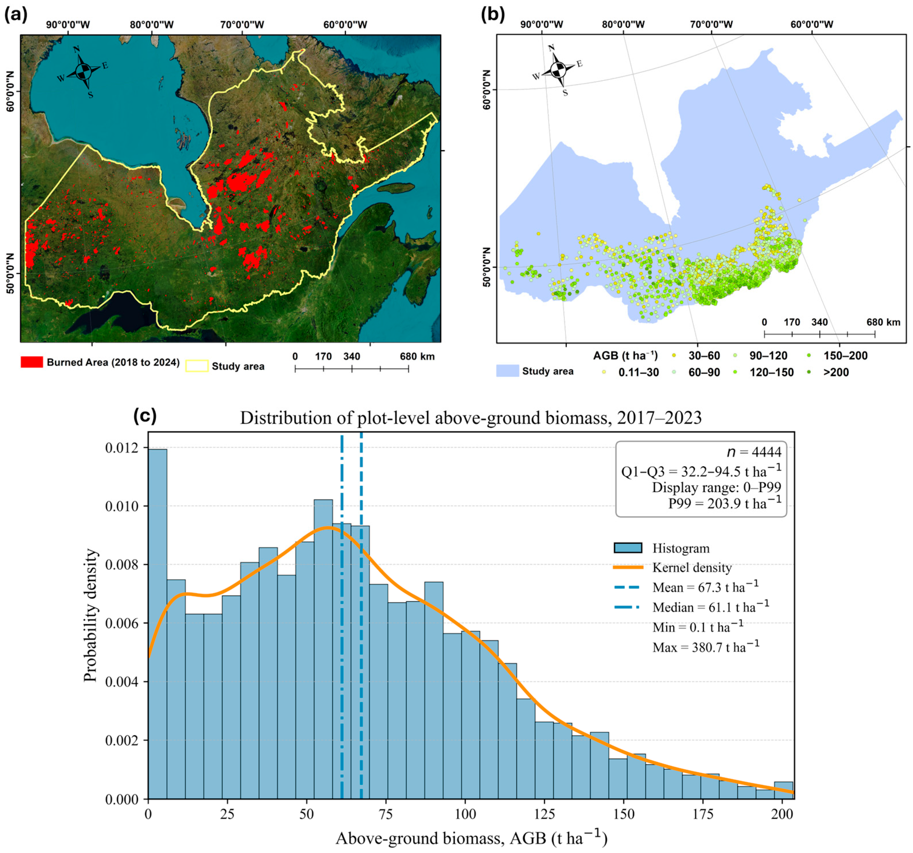
The study was conducted across the boreal forest region of Quebec and Ontario, Canada (Figure 1a) and covered approximately 175 million hectares. The region encompasses substantial climatic, topographic, and ecological gradients, and includes needleleaf forest, broadleaf deciduous forest, mixed forest, shrubland, grassland, and wetland ecosystems affected by recurrent wildfires and other disturbances [3,37]. This environmental heterogeneity provides an appropriate setting for evaluating multi-source predictors of AGB across a broad range of forest and site conditions.

Reference AGB data were obtained from permanent sample plot (PSP) forest inventories compiled between 2017 and 2023 [6]. Tree-level AGB was derived from forest-inventory measurements using the procedures and species-specific allometric equations reported in [6] and was aggregated to the plot scale (t ha⁻¹). Each record represented one plot-year observation and included a field-derived AGB estimate, geographic coordinates, observation year, reported plot area, and a unique physical-plot identifier (PlotName). The initial dataset contained 4444 plot-year observations distributed across the study area (Figure 1b). Some physical plots were measured in more than one year; consequently, observations from different years could share the same PlotName. This repeated-observation structure was accounted for through the grouped cross-validation procedure described in Section 2.4.

The initial reference dataset showed substantial variation in AGB among plot-year observations, reflecting differences in forest structure, stand condition, and disturbance history across the study area [6]. AGB values ranged from 0.1 to 380.7 t ha⁻¹, with a mean of 67.3 t ha⁻¹ and an interquartile range of 32.2–94.5 t ha⁻¹ (Figure 1c). The distribution was right-skewed. To limit the visual influence of extreme high-biomass observations, the histogram and kernel-density curve were displayed only up to the 99th percentile (203.9 t ha⁻¹). The broad range of AGB values allowed for the evaluation of model performance across heterogeneous forest conditions.

For each plot-year record, remote-sensing, environmental, and geographic predictors were extracted for the corresponding location and observation year and linked to the field-derived AGB estimate. Records lacking a valid AGB value or PlotName, or those that could not be linked to the predictor data required for model development, were excluded before modeling. Missing values in individual numeric predictors among the retained records were handled through the fold-specific preprocessing described in Section 2.4.

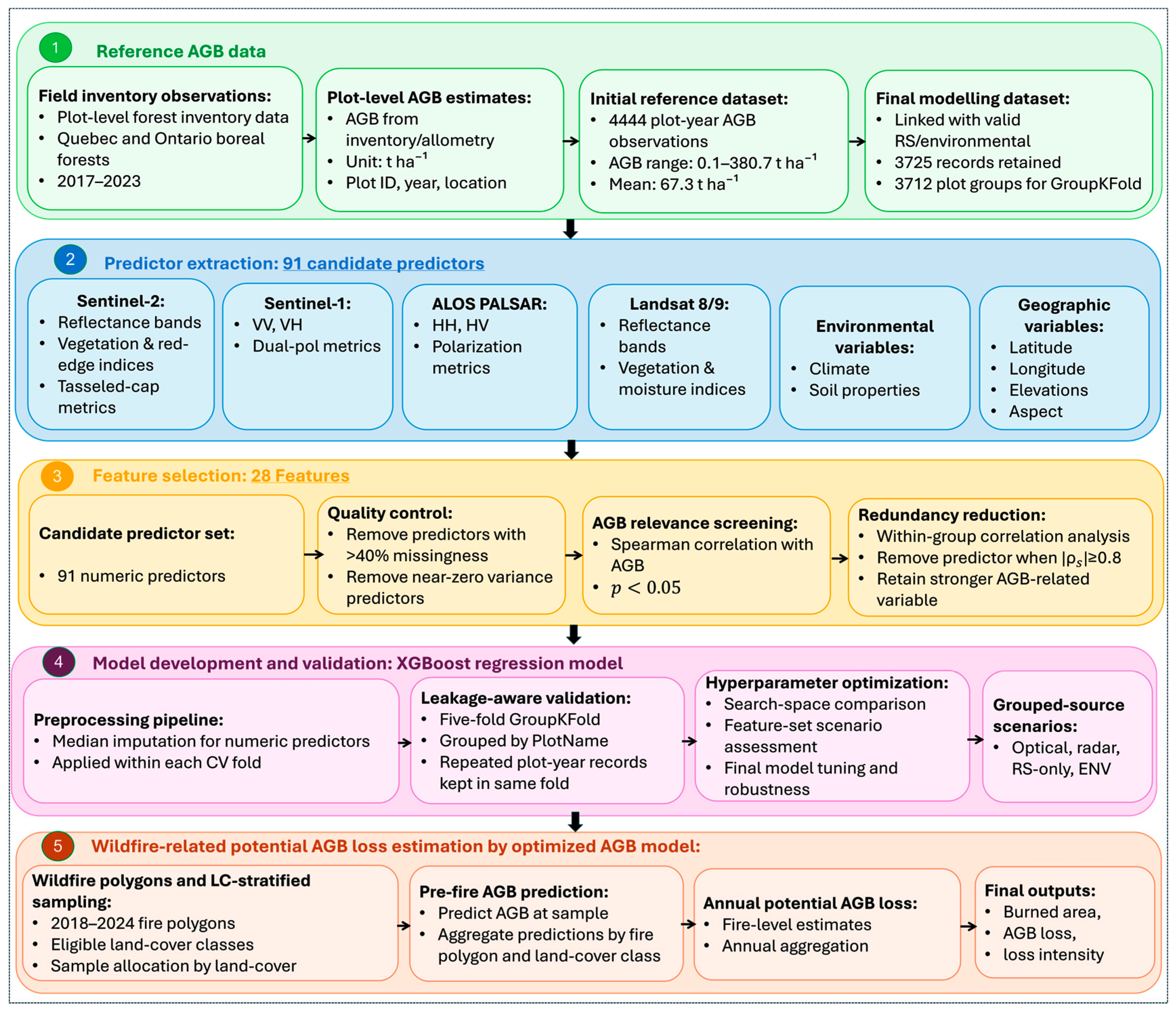
The overall methodological workflow is summarized in Figure 2. It includes the preparation of the reference AGB dataset, extraction of multi-source predictors, product-wise feature selection, extreme gradient boosting (XGBoost) model development using grouped cross-validation, staged assessment of hyperparameter and predictor-source configurations, final model optimization, and estimation of annual wildfire-related potential AGB loss.

2.2. Remote Sensing and Environmental Predictors

Multi-source predictors were extracted primarily using Google Earth Engine (GEE; Google LLC, Mountain View, CA, USA) and matched to the year and location of each reference AGB observation. The candidate predictor set included optical, C- and L-band synthetic aperture radar (SAR), topographic, soil, climate, and geographic variables. Complete predictor names, abbreviations, source products, and formulas are provided in

Table A1. Candidate remote-sensing and environmental/geographic predictors and plot-level extraction and quality-control variables used in the AGB-modeling workflow. Note: Formulas follow the Google Earth Engine implementation used in this study. Band symbols are sensor-specific: for Sentinel-2, B2 = blue, B3 = green, B4 = red, B5–B7 = red-edge, B8 = NIR, B8A = narrow NIR, B11 = SWIR1, and B12 = SWIR2. For Landsat 8/9, BLUE, GREEN, RED, NIR, SWIR1, and SWIR2 indicate harmonized surface reflectance bands. An epsilon term was used in the code to avoid division by zero but is omitted from formulas for readability. References are representative sources for the index, dataset, or their use in AGB modeling. Bold text and shaded backgrounds identify the different predictor groups. The asterisk (*) represents the corresponding climate-variable prefix; “*_base” and “*_anom” denote the baseline and anomaly versions of each climate variable, respectively.

Predictors Group	Full Name/Metric	Formula or Definition	Biophysical Meaning	Representative References
Sentinel-2 optical predictors
B2, B3, B4, B5, B6, B7, B8, B8A, B11, B12	Sentinel-2 surface reflectance bands	Scaled BOA reflectance bands: blue, green, red, red-edge, NIR, narrow NIR, SWIR1, SWIR2	Spectral response related to canopy greenness, chlorophyll, water content, and forest structure.	[17,34,58]
NDVI	Normalized Difference Vegetation Index	(B8 − B4)/(B8 + B4)	Canopy greenness, photosynthetic activity, and vegetation density.	[17,59]
GNDVI	Green Normalized Difference Vegetation Index	(B8 − B3)/(B8 + B3)	Green-band chlorophyll sensitivity and canopy vigor.	[35,60]
DVI	Difference Vegetation Index	B8 − B4	Absolute NIR-red contrast associated with vegetation amount.	[35,61]
EVI	Enhanced Vegetation Index	2.5 × (B8 − B4)/(B8 + 6B4 − 7.5B2 + 1)	Vegetation vigor with reduced atmospheric and soil-background effects.	[34,62]
MCARI	Modified Chlorophyll Absorption Ratio Index	[(B5 − B4) − 0.2(B5 − B3)] × (B5 − B4)	Chlorophyll absorption and red-edge response.	[17,63]
S2REP	Sentinel-2 Red-Edge Position	705 + 35 × [((B4 + B7)/2 − B5)/(B6 − B5)]	Red-edge position related to chlorophyll and canopy condition.	[34,64]
REIP	Red-Edge Inflection Point	700 + 40 × [((B4 + B7)/2 − B5)/(B6 − B5)]	Red-edge inflection and chlorophyll-sensitive canopy status.	[64,65]
CCCI	Canopy Chlorophyll Content Index	[(B8 − B6)/(B8 + B6)]/[(B8 − B4)/(B8 + B4)]	Relative canopy chlorophyll content and nitrogen/chlorophyll status.	[18,66]
CIRE	Chlorophyll Index Red Edge	(B8/B6) − 1	Chlorophyll-sensitive red-edge index.	[18,67]
CVI	Chlorophyll Vegetation Index	(B8 × B4)/(B32)	Chlorophyll and canopy vigor proxy.	[17,68]
GLI	Green Leaf Index	(2B3 − B4 − B2)/(2B3 + B4 + B2)	Green vegetation fraction and visible-band greenness.	[69]
GRNDVI	Green-Red Normalized Difference Vegetation Index	(B8 − (B3 + B4))/(B8 + B3 + B4)	Combined green-red contrast for vegetation condition.	[35,70]
BWDRVI	Blue Wide Dynamic Range Vegetation Index	(0.1B8 − B2)/(0.1B8 + B2)	Wide dynamic range greenness index using blue and NIR response.	[71]
NDVIRE	Normalized Difference Vegetation Index Red Edge	(B8 − B7)/(B8 + B7)	Red-edge vegetation condition and chlorophyll sensitivity.	[34,60]
WDVI	Weighted Difference Vegetation Index	B8 − 0.5B4	Soil-adjusted NIR-red contrast and vegetation amount.	[72]
TCB	Tasseled Cap Brightness	0.3510B2 + 0.3813B3 + 0.3437B4 + 0.7196B8 + 0.2396B11 + 0.1949B12	Overall scene/canopy brightness and soil/background contribution.	[73,74]
TCW	Tasseled Cap Wetness	0.2578B2 + 0.2305B3 + 0.0883B4 + 0.1071B8 − 0.7611B11 − 0.5308B12	Canopy and surface moisture response.	[73,74]
TCG	Tasseled Cap Greenness	−0.3599B2 − 0.3533B3 − 0.4734B4 + 0.6633B8 + 0.0087B11 − 0.2856B12	Vegetation greenness and canopy photosynthetic signal.	[73,74]
TCA	Tasseled Cap Angle	atan2(TCG, TCB)	Angular relation between greenness and brightness.	[74,75]
TCD	Tasseled Cap Distance	sqrt(TCB2 + TCG2)	Magnitude of brightness-greenness response.	[74,75]
Landsat 8/9 optical predictors
BLUE, GREEN, RED, NIR, SWIR1, SWIR2	Harmonized Landsat surface reflectance bands	Scaled C2 L2 surface reflectance bands: DN × 0.0000275 − 0.2	Spectral response related to greenness, canopy water, disturbance, and structure.	[34,38]
NDVI	Normalized Difference Vegetation Index	(NIR − RED)/(NIR + RED)	Canopy greenness and vegetation density.	[19,59]
EVI	Enhanced Vegetation Index	2.5 × (NIR − RED)/(NIR + 6RED − 7.5BLUE + 1)	Vegetation vigor with reduced atmospheric and soil-background effects.	[34,62]
SAVI	Soil-Adjusted Vegetation Index	1.5 × (NIR − RED)/(NIR + RED + 0.5)	Canopy greenness with soil-background adjustment.	[17,76]
DVI	Difference Vegetation Index	NIR − RED	NIR-red vegetation contrast.	[61]
RVI	Ratio Vegetation Index	NIR/RED	Vegetation amount and biomass-related greenness ratio.	[61,77]
ARVI	Atmospherically Resistant Vegetation Index	[NIR − (2RED − BLUE)]/[NIR + (2RED − BLUE)]	Vegetation greenness with partial atmospheric resistance.	[78]
NDMI/NDWI_Gao	Normalized Difference Moisture Index/Gao NDWI	(NIR − SWIR1)/(NIR + SWIR1)	Canopy water content and vegetation moisture.	[29,79]
MSI	Moisture Stress Index	SWIR1/NIR	Vegetation water stress and canopy moisture condition.	[80]
NBR	Normalized Burn Ratio	(NIR − SWIR2)/(NIR + SWIR2)	Disturbance, canopy moisture, and fire-related structural change.	[7,56]
NBR2	Normalized Burn Ratio 2	(SWIR1 − SWIR2)/(SWIR1 + SWIR2)	Moisture and post-disturbance surface/vegetation response.	[56]
NIRv	Near-Infrared Reflectance of Vegetation	NDVI × NIR	Proxy for canopy structure, vegetation productivity, and photosynthesis.	[81]
NDPI	Normalized Difference Phenology Index	[NIR − (0.74RED + 0.26SWIR1)]/[NIR + (0.74RED + 0.26SWIR1)]	Vegetation phenology and reduction in soil/snow/background effects.	[82]
SATVI	Soil-Adjusted Total Vegetation Index	1.5 × (SWIR1 − RED)/(SWIR1 + RED + 0.5) − SWIR2/2	Senescence, dry vegetation, and soil/background effects.	[83]
PSRI	Plant Senescence Reflectance Index	(RED − GREEN)/NIR	Plant senescence, carotenoid/chlorophyll changes, and stress response.	[84]
Sentinel-1 C-band SAR and ALOS L-band SAR predictors
VVg0, VHg0	Sentinel-1 gamma-nought backscatter	VVg0 = 10^(VV_dB/10)/cos(theta); VHg0 = 10^(VH_dB/10)/cos(theta)	Radiometrically normalized C-band backscatter related to canopy structure and moisture.	[22,85]
VVVH_ratio	Sentinel-1 VV/VH ratio	VVg0/VHg0	Dual-polarization contrast related to canopy structure and scattering mechanisms.	[22,23]
VVminusVH	Sentinel-1 VV minus VH difference	VVg0 − VHg0	Polarization difference related to canopy/woody scattering contrast.	[21,23]
RVI	Sentinel-1 Radar Vegetation Index	4VHg0/(VVg0 + VHg0)	Vegetation structure and depolarization response.	[86,87]
HHg0 (dB), HVg0(dB)	ALOS gamma-nought backscatter in decibels	gamma0_dB = 10 × log10(DN2) − 83	L-band backscatter related to woody components and canopy structure.	[29,88]
HHg0_(linear), HVg0_(linear)	ALOS gamma-nought backscatter in linear units	gamma0_linear = 10^(gamma0_dB/10)	Linear L-band backscatter for ratio, difference, and RVI calculations.	[23,88]
HH_HV_ratio	ALOS HH/HV ratio	HHg0_(linear)/HVg0_(linear)	L-band polarization contrast related to canopy structure and woody biomass.	[23,29]
HHminusHV	ALOS HH minus HV difference	HHg0 (linear) − HVg0 (linear)	L-band polarization difference related to scattering contrast.	[21,23]
RVI	ALOS Radar Vegetation Index	4HVg0 (linear)/(HHg0 (linear) + HVg0 (linear))	Vegetation structure and depolarization response from L-band SAR.	[29,87]
Environmental and plot-level extraction variables
elev_m	Elevation	Copernicus GLO-30 DEM elevation	Topographic control on climate, species distribution, and productivity.	[36]
slope_deg	Slope	Terrain slope derived from DEM	Terrain gradient influencing soil moisture, drainage, and productivity.	[29,36]
aspect_deg	Aspect	Terrain aspect derived from DEM	Solar exposure and microclimatic control.	[29,36]
lon, lat	Longitude and latitude	Pixel longitude and latitude	Spatial gradients and geographic location context.	[34,36]
soc_0_5	Soil organic carbon, 0–5 cm	Mean SoilGrids SOC at 0–5 cm	Soil carbon and fertility conditions influencing productivity.	[40,89]
n_0_5	Soil nitrogen, 0–5 cm	Mean SoilGrids nitrogen at 0–5 cm	Nutrient availability and site fertility.	[40,89]
clay_0_5, sand_0_5, silt_0_5	Soil texture fractions, 0–5 cm	Mean SoilGrids clay, sand, and silt fractions at 0–5 cm	Soil water retention, drainage, and rooting environment.	[40,89]
TEM_yr_c	Annual mean temperature	(tmin + tmax)/2, averaged annually	Thermal regime and productivity control.	[36,41]
PRE_yr_mm	Annual precipitation	sum(monthly precipitation), Jan–Dec	Moisture availability and productivity control.	[36,41]
TEM_grow_c	Growing-season mean temperature	mean monthly temperature, May–Sep	Growing-season thermal conditions.	[41]
PRE_grow_mm	Growing-season precipitation	sum monthly precipitation, May–Sep	Growing-season moisture availability.	[41]
AT0_grow	Accumulated temperature above 0 °C	sum[max(Tmean, 0) × days in month], May–Sep	Growing-season heat accumulation.	[41]
AT10_grow	Accumulated temperature above 10 °C	sum[max(Tmean − 10, 0) × days in month], May–Sep	Growing-degree proxy for boreal vegetation growth.	[41]
*_base	Long-term climate baseline	mean climate metric over baseline years	Climatological site condition.	[41]
*_anom	Climate anomaly	year-specific climate metric − baseline metric	Interannual climate departure from baseline conditions.	[41]
r_eff_m	Effective plot buffer radius	r = sqrt(A/pi), where A = plot area in m2; r_eff = max(r, 45 m)	Adaptive plot-scale support for 30 m remote sensing extraction.	This study
valid_frac	Valid-data fraction	mean(valid_mask) within plot buffer	Quality-control measure indicating the fraction of valid pixels used in extraction.	This study
is_valid	Valid observation flag	valid_frac > threshold	Indicator used to identify usable plot-year predictor records.	This study

.

Optical predictors were derived from Sentinel-2 Surface Reflectance Harmonized imagery and Landsat 8/9 Collection 2 Level-2 surface-reflectance imagery. Pixels affected by clouds, cloud shadows, cirrus, snow, saturation, or other low-quality conditions were excluded using the respective quality-assurance (QA) layers. For each year, median composites were generated for July–August to represent peak growing-season conditions. The initial optical pool comprised 30 Sentinel-2 variables and 21 Landsat variables, including surface reflectance bands, vegetation indices, red-edge metrics, moisture- and disturbance-sensitive indices, and tasseled cap components. These variables represent complementary spectral responses related to canopy condition, vegetation vigor, moisture, and forest structure [15,17,18,26,34,38].

SAR predictors were derived from two data sources representing different radar wavelengths: Sentinel-1 C-band observations and annual ALOS PALSAR/PALSAR-2 L-band mosaics. For the C-band predictors, VV and VH observations were radiometrically normalized to gamma-nought backscatter. The five-candidate C-band variables comprised VV and VH backscatter and three derived dual-polarization metrics, which provided information related to canopy structure, scattering behavior, and vegetation moisture conditions [21,22]. For the L-band predictors, HH and HV polarization data were used. Digital numbers were converted to gamma-nought backscatter in decibels (dB) and linear units, from which polarization ratios, differences, and radar vegetation metrics were calculated. Seven candidate L-band variables were initially considered. The longer L-band wavelength provides greater sensitivity to woody components and complements the shorter-wavelength C-band response [23,29].

The environmental predictor group contained 28 topographic, soil, climate, and geographic variables. Elevation, slope, and aspect were derived from the Copernicus DEM GLO-30 [39]. Near-surface soil organic carbon, total nitrogen, and clay, sand, and silt fractions were obtained from SoilGrids [36,40]. Climate variables were derived from TerraClimate and included annual and May–September precipitation and temperature metrics and accumulated growing-season temperature indices [41]. For each climate metric, a 2000–2024 reference-period mean was calculated from TerraClimate, and annual anomalies were expressed as the difference between the value for a plot-observation year and the corresponding reference mean. Longitude and latitude were included to represent broad geographic gradients in forest and environmental conditions [36].

Optical and radar variables were harmonized to a 30 m grid in the NAD83/Canada Atlas Lambert projection (EPSG:3978). Predictor values were summarized within an adaptive circular buffer centered on each plot. Assuming a circular plot, the nominal buffer radius was calculated as r = √(A/π), where A is the reported plot area in square meters. A minimum radius of 45 m was imposed to provide sufficient spatial support for the 30 m imagery and reduce sensitivity to plot–pixel misregistration. Environmental variables were extracted using spatial supports corresponding to their native or effective resolutions: 30 m for topographic variables, 250 m for soil variables, and 4 km for climate variables. Water pixels were excluded where applicable using the North American Land Change Monitoring System (NALCMS) land-cover layer [42]. Valid-data masks and the proportion of valid pixels within each extraction buffer were recorded to identify incomplete plot-year observations. In total, 91 candidate numeric predictors were assembled before feature selection.

2.3. Feature Selection and Feature-Set Construction

A product-wise feature selection procedure was applied to reduce irrelevant and redundant predictors while preserving representation from each data source. Selection was conducted separately for Sentinel-2, Landsat 8/9, Sentinel-1, ALOS PALSAR/PALSAR-2, and environmental/geographic predictors.

Within each numeric predictor group, variables with more than 40% missing observations or near-zero variance, operationally defined as a variance $\le 1\times {10}^{-12}$, were first removed. The 40% missingness threshold was specified a priori to exclude poorly represented predictors while retaining variables with sufficient observations for subsequent screening. The remaining variables were screened using Spearman rank correlation with plot-level AGB. Predictors were retained when their association with AGB was statistically significant at $p<0.05$. Spearman correlation was used because it evaluates monotonic associations without requiring linear biomass–predictor relationships [5,36].

Redundancy was then evaluated separately within each predictor group using pairwise Spearman correlations. When two retained predictors were strongly correlated ($\left|{\rho }_s\right|\ge 0.80$, where ${\rho }_s$ denotes Spearman’s rank correlation coefficient), the predictor with the weaker absolute correlation with AGB was removed. Thus, each correlated pair was resolved using its relative association with the response variable rather than by arbitrary variable order. This procedure reduced overlap among related spectral bands, vegetation indices, polarization metrics, and environmental variables while avoiding direct competition among physically distinct data sources [21,29,34,36]. The $\left|{\rho }_s\right|$= 0.80 cutoff was specified a priori as a pragmatic criterion for strong monotonic redundancy, balancing the removal of near-duplicate variables against the retention of complementary information from physically distinct predictor sources [5]. Variance inflation factors were not used in the feature-pruning procedure; therefore, no VIF cutoff was applied.

The final predictors retained from each product group were used to construct the full multi-source feature set, as well as the source-specific and source-removal feature sets. These configurations were subsequently compared to evaluate changes in predictive performance associated with the inclusion or removal of optical, radar, environmental, and geographic predictor groups. The full multi-source feature set was then used for final hyperparameter optimization.

Because the original product-wise feature-selection procedure was applied to the complete modeling dataset before cross-validation, we additionally assessed the potential influence of information leakage associated with response-informed predictor selection. In this sensitivity analysis, the complete product-wise selection procedure was repeated independently within each training subset of the five-fold GroupKFold framework. Missingness and variance screening, Spearman association testing with AGB, and within-group correlation-based redundancy pruning were therefore performed using the training observations only. The resulting fold-specific predictor sets were then used to fit the models and generate predictions for the corresponding held-out validation folds. For this sensitivity comparison, fold assignments, XGBoost hyperparameters, preprocessing procedures, and all other modeling settings were held constant.

2.4. Model Development, Spatial Validation, Applicability-Domain Assessment, and Evaluation Metrics

Plot-level AGB was modeled using extreme gradient boosting regression (XGBoost version 2.1.4; XGBoost Developers) [43]. Each observation represented one plot-year record. AGB (t ha⁻¹) was the response variable, while the selected variables were used as predictors. XGBoost was selected because it can represent nonlinear relationships and interactions among heterogeneous optical, SAR, environmental, and geographic predictors and has performed effectively in previous remote-sensing-based biomass applications [32,34,35].

Before model fitting, observations with missing AGB values or plot-group identifiers were removed. Within each cross-validation fold, missing numeric predictor values were imputed using medians estimated from the training subset. This imputation was embedded within the modeling pipeline so that its parameters were learned exclusively from the training data and then applied to the corresponding validation subset.

Model performance was evaluated using five-fold grouped cross-validation, implemented with the GroupKFold splitter in scikit-learn version 1.6.1 (scikit-learn Developers) [44]. PlotName was used as the grouping variable because it identified each physical sampling location. All records sharing the same PlotName, including repeated plot-year observations, were assigned to the same fold, preventing records from a given plot from occurring in both the training and validation subsets. This design reduced information leakage from repeated observations and provided a more conservative assessment of generalization to previously unseen plots than random record-level partitioning [45]. However, it should not be interpreted as geographically blocked spatial cross-validation. For each iteration, the model was trained on four folds and evaluated on the remaining fold, with held-out predictions retained as out-of-fold predictions. The same fold assignments were reused for the search-space comparison, feature-set assessment, final Optuna optimization, and seed-robustness analysis so that differences among model configurations were not confounded by changes in data partitioning.

Following final model optimization, north–south geographic transferability was evaluated using a matched latitudinal-block cross-validation analysis, consistent with recommendations for evaluating models with spatially structured data [45]. A representative latitude was assigned to each physical plot by using the median latitude of all records sharing the same PlotName. Plot groups were ordered from south to north and divided into five contiguous latitudinal blocks containing approximately equal numbers of physical plots. Each block was held out once for validation while the model was fitted using the remaining four blocks, with the northernmost block providing a direct assessment of northward geographic transferability. The final predictor configuration, preprocessing pipeline, and optimized XGBoost hyperparameters were held constant, and neither feature selection nor hyperparameter optimization was repeated. To select the number of boosting iterations without using the outer validation block, a single GroupShuffleSplit partition was created within each outer training set, with 15% of the unique PlotName groups reserved as an internal early-stopping subset [44]. All records sharing the same PlotName were retained within the same inner subset. The selected number of boosting iterations was then used to refit the model on the complete outer training set before predicting the held-out block. For direct comparison, the conventional five-fold PlotName GroupKFold assessment was repeated using the same model inputs, preprocessing, hyperparameters, inner early-stopping procedure, and refitting strategy, so that the outer validation partitioning scheme was the only intended difference between the two assessments. Because longitude was retained among the final predictors, a paired sensitivity analysis was conducted to assess whether model performance depended strongly on explicit geographic location. Within each original PlotName-grouped cross-validation fold, longitude was replaced by the median longitude of the corresponding training subset in both the training and validation data, thereby removing its spatial variation while preserving the original input structure. The full and longitude-neutralized models were refitted using identical fold assignments, preprocessing, optimized hyperparameters, random seed, and fitting procedures.

To further characterize the model’s applicability domain at the wildfire sample locations, we compared the distributions of the 14 final environmental/geographic predictors between the 3725 plot-year modeling observations and the 9937 wildfire sample points. For each predictor, we calculated the proportion of wildfire points below, within, and above the univariate minimum–maximum range represented by the modeling data. We additionally calculated the proportion of complete-case wildfire points falling within the training ranges of all 14 predictors and the mean number of out-of-range predictors per point.

Root mean square error (RMSE; t ha⁻¹) was used as the primary optimization and evaluation metric because it reports error in the same units as AGB and gives greater weight to larger deviations. Mean absolute error (MAE; t ha⁻¹), the coefficient of determination (R²), and mean prediction bias were reported as complementary measures [46,47]. Relative RMSE was calculated as RMSE divided by the mean observed AGB and expressed as a percentage, consistent with previous remote-sensing-based AGB studies [36,48]. Normalized RMSE (nRMSE) was calculated by dividing RMSE by the observed AGB range and expressing the result as a percentage. Overall metrics were calculated from the pooled out-of-fold predictions, whereas model-comparison metrics were reported as mean ± standard deviation across the five grouped folds.

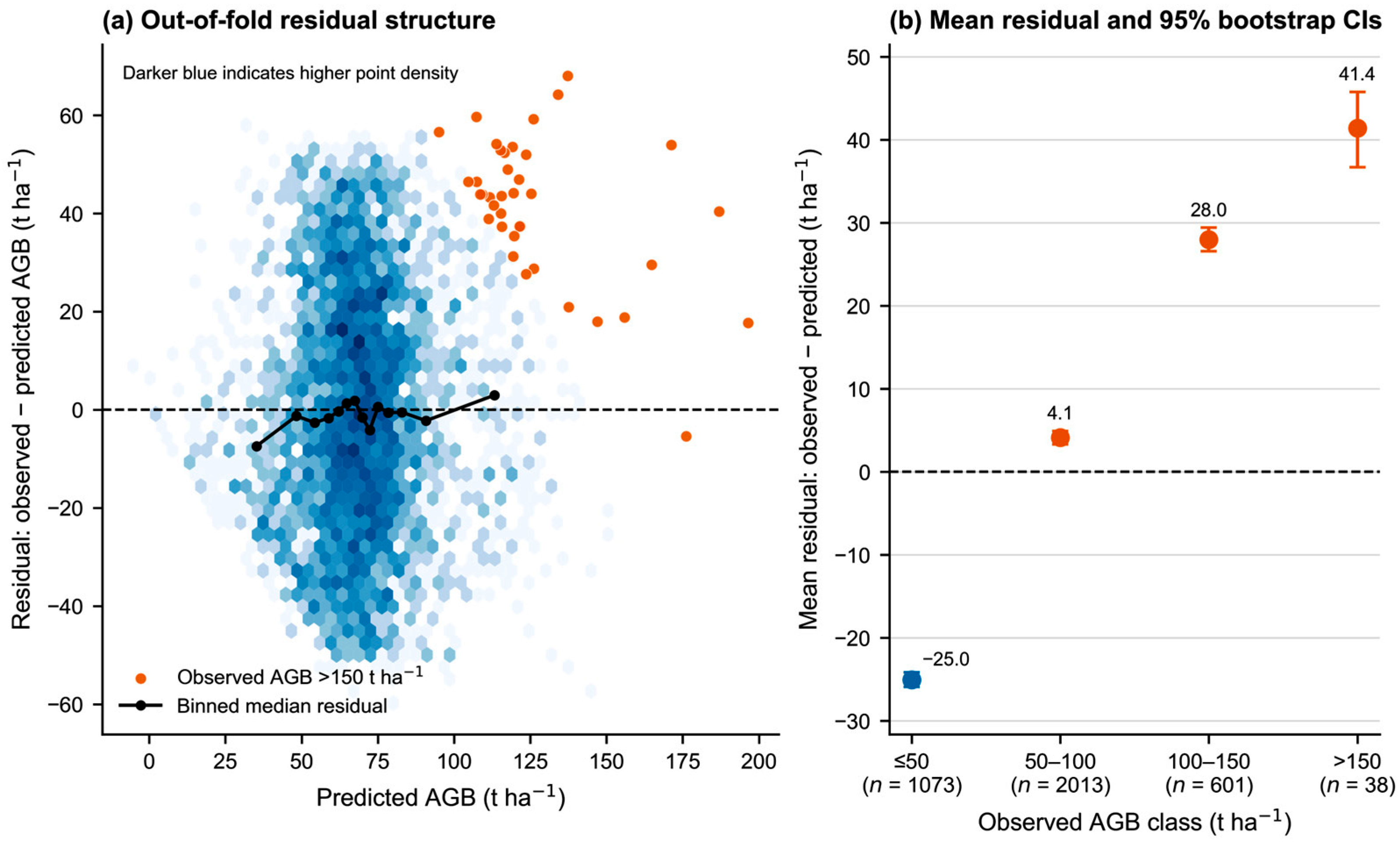
To further characterize error heterogeneity across the observed biomass range, residual diagnostics were performed using the pooled out-of-fold predictions. Residuals were defined as observed minus predicted AGB, such that positive values indicate underestimation and negative values indicate overestimation. Residuals were plotted against predicted AGB, and observations were stratified according to observed AGB into four classes: ≤50, 50–100, 100–150, and >150 t ha⁻¹. For each class, mean observed and predicted AGB, RMSE, relative RMSE, and mean residual were calculated. Relative RMSE was obtained by dividing the class-specific RMSE by the corresponding mean observed AGB and expressing the result as a percentage. Uncertainty in the class-specific mean residual was quantified using 5000 nonparametric bootstrap resamples drawn with replacement within each AGB class. The 95% bootstrap percentile intervals were defined by the 2.5th and 97.5th percentiles of the bootstrap distributions [49].

2.5. Model Tuning, Feature-Set Assessment, and Robustness

All model-comparison experiments used the same modeling dataset, preprocessing pipeline, five-fold grouped cross-validation partitions, and evaluation metrics described in Section 2.4. First, two candidate XGBoost hyperparameter search spaces were compared while holding the full predictor set and fold assignments constant. The baseline-like space was evaluated using 220 randomly sampled configurations, and the expanded space was evaluated using 500 configurations. Random sampling was used because it can explore influential hyperparameters more efficiently than exhaustive grid search when only a subset of settings strongly affects model performance [50]. The evaluated parameters controlled the number of boosting trees, learning rate, tree depth, minimum child weight, row and column subsampling, minimum split-loss reduction, L1 and L2 regularization, and histogram bin size [43]. Early stopping was applied within each validation fold. Configurations were ranked by mean grouped-validation RMSE, with MAE and R² retained as secondary criteria; the complete search domains are reported in

Table A2. XGBoost hyperparameter search domains and final optimized values. This table summarizes the hyperparameter domains used in the staged optimization workflow and the values selected by the best-performing Optuna trial. Scenario 01 compared alternative hyperparameter search spaces using random sampling, whereas Scenario 03 performed final Optuna-based tuning of the full multi-source feature set under five-fold GroupKFold cross-validation. Note: Scenario 03 used the Tree-structured Parzen Estimator sampler. The final implementation used histogram-based tree construction (tree_method = hist), GPU acceleration (device = cuda), four parallel CPU threads (n_jobs = 4), and 100 early-stopping rounds.

Hyperparameter	Model Role	Scenario 01: Search-Space Comparison	Scenario 03: Final Optuna Search Domain	Final Optimized Value
Number of boosting trees (n_estimators)	Controls the number of sequential trees.	300–4000, depending on search space	1000–4000; step = 100	2600
Learning rate (learning_rate)	Controls the contribution of each tree.	0.003–0.100, depending on search space	0.002–0.020; log scale	0.014789
Maximum tree depth (max_depth)	Controls tree complexity.	2–18, depending on search space	3–6	4
Minimum child weight (min_child_weight)	Controls minimum weight required in a leaf.	1–30, depending on search space	1–10	5
Row subsampling (subsample)	Controls fraction of observations used per tree.	0.50–1.00, depending on search space	0.60–1.00; step = 0.05	0.75
Column subsampling (colsample_bytree)	Controls fraction of predictors used per tree.	0.50–1.00, depending on search space	0.40–0.90; step = 0.05	0.45
Split-loss reduction (gamma)	Minimum loss reduction required for a split.	0.00–2.00, depending on search space	0.00–0.50; step = 0.05	0.00
L1 regularization (reg_alpha)	Adds sparsity penalty to reduce overfitting.	0.00–10.00, depending on search space	0 or 1 × 10−4–3.0; log scale	0.00
L2 regularization (reg_lambda)	Adds shrinkage penalty to reduce overfitting.	0.50–100.00, depending on search space	1.00–15.00; log scale	2.425969
Histogram bins (max_bin)	Controls resolution of histogram-based tree construction.	128, 192, 256, 384, or 512; baseline used 256	192, 256, or 384	384
Early stopping rounds	Stops boosting when validation performance no longer improves.	100	100	100

.

Using the best-performing configuration from the retained search space, feature-set configurations were compared to evaluate changes in predictive performance associated with the inclusion or removal of predictor sources. Scenarios included the full multi-source set, leave-one-source-out configurations, source-only models, and grouped optical, radar, remote-sensing, and environmental combinations. Optical–environmental and radar–environmental configurations were also assessed to examine complementarity among predictor types, consistent with previous multi-source AGB studies [21,29,34,35,51]. Hyperparameters were held constant across scenarios so that performance differences reflected predictor-set composition rather than model complexity.

Final hyperparameter optimization of the full multi-source feature set was conducted with the Optuna version 4.9.0 (Optuna Developers) framework using the Tree-structured Parzen Estimator (TPE) sampler [52,53]. The study comprised 303 completed trials evaluated with the same grouped cross-validation framework, and mean validation RMSE was used as the optimization objective. The parameter domains and implementation settings, including early stopping, are provided in Table A2. Finally, robustness to stochastic variation was assessed using random seeds 42, 123, and 2025 while holding the dataset, predictor configuration, fold assignments, and optimized hyperparameters constant. Seed-specific RMSE, MAE, and prediction bias were compared, and the optimized model was subsequently used to estimate wildfire-related potential AGB loss.

2.6. Annual Wildfire-Related Potential AGB Estimation, Sampling Uncertainty, and Sensitivity Analyses

The optimized model was applied to land-cover-stratified sample points within mapped wildfire polygons in Quebec and Ontario for 2018–2024 [11] (Figure 1a). This sampling approach was used instead of wall-to-wall prediction to reduce computational demands and to estimate mean AGB density for each land-cover class within each fire polygon.

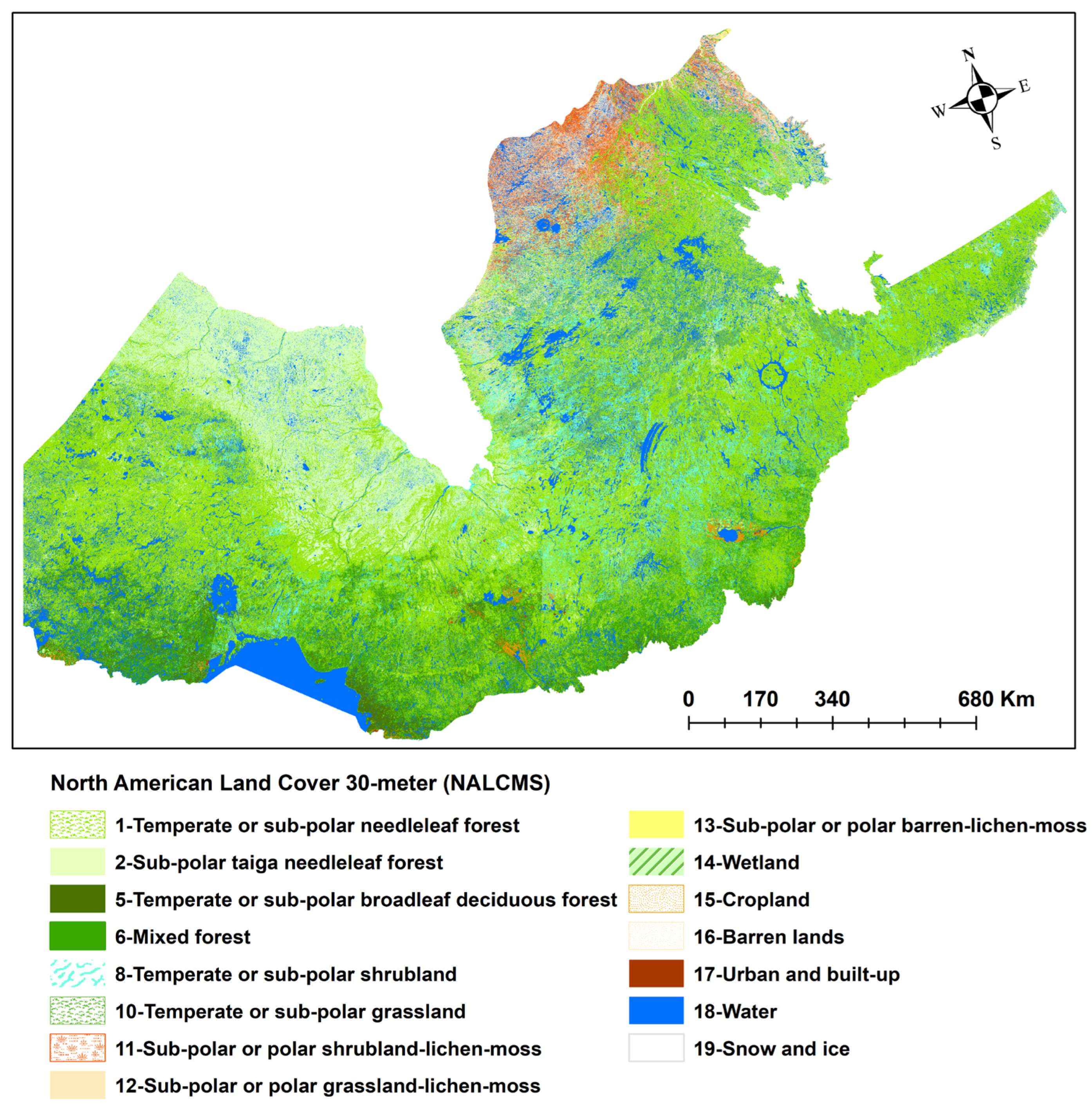
Land-cover information was obtained from the 2020 NALCMS 30 m product [42] (Figure A1). The NALCMS comprises 19 classes, of which 15 are represented in the Canadian product, as tropical classes 3, 4, 7, and 9 are absent. Classes 1–14 were considered eligible for the wildfire analysis. The 10 eligible classes represented within the study area comprised two needleleaf forest classes, broadleaf deciduous forest, mixed forest, shrubland, grassland, three sub-polar or polar lichen–moss classes, and wetland. Classes 15–19—cropland, barren land, urban and built-up areas, water, and snow and ice—were excluded as non-target classes.

For each fire polygon, effective burned area was defined as the total area of 30 m NALCMS pixels assigned to eligible land-cover classes. Contiguous land-cover fragments smaller than 1 ha were excluded before sample allocation. The target sample size for each polygon was determined at a density of one point per 50 ha of effective burned area. A minimum of 30 and a maximum of 400 points per polygon was imposed to maintain representation in relatively small fires while limiting the computational influence of very large polygons. Points were allocated among eligible land-cover classes in proportion to their area within each polygon, subject to a minimum of two and a maximum of 80 points per class. These class-level limits maintained representation of minor eligible classes while avoiding excessive sampling of dominant classes, yielding a total of 9937 wildfire sample points.

To estimate potential pre-fire biomass, time-varying predictors were extracted for each sample point from the calendar year preceding the fire (y − 1), while static predictors retained their original values. The optimized model was then used to predict potential pre-fire AGB density at each sample point (t ha⁻¹). Predictions were summarized by fire year y, land-cover class c, and fire polygon f. Potential AGB loss for each year–class–polygon combination was calculated as:

$$L_{y,c,f}={\widehat{B}}_{y,c,f}\times A_{y,c,f}$$

(1)

where $L_{y,c,f}$ is the potential AGB loss in tonnes for year $y$, land-cover class $c$, and fire polygon $f$; ${\widehat{B}}_{y,c,f}$ is the mean model-predicted AGB density in t ha⁻¹ for sampled points within that combination; and $A_{y,c,f}$ is the corresponding effective burned area (ha). Annual potential biomass loss was calculated by summing across all eligible land-cover classes and fire polygons:

$$L_y={\sum }_f{\sum }_c{\widehat{B}}_{y,c,f}\times A_{y,c,f}$$

(2)

Annual potential AGB loss intensity was defined as the potential AGB loss per unit of effective burned area.

$$I_y={\displaystyle \frac{L_y}{A_y}},$$

(3)

where $A_y={\sum }_f{\sum }_c{A}_{y,c,f}$ is the total effective burned area in year $y$. Accordingly, $I_y$, expressed in t ha⁻¹, represents the area-weighted mean potential AGB exposure within eligible burned areas. This metric was used to distinguish annual variation in the biomass density of burned landscapes from variation driven primarily by total fire extent.

Finite-point sampling uncertainty was evaluated using a polygon-level nonparametric bootstrap [54]. Within each polygon, predicted AGB values were resampled with replacement using the original polygon-specific sample size. For each of 5000 bootstrap replicates, the resampled polygon mean was multiplied by its effective eligible area, and the resulting polygon-level pseudo-totals were summed by year. Because the baseline annual estimates incorporated land-cover-specific area weights, the relative variation between each bootstrap pseudo-total and its full-sample counterpart was applied to the corresponding baseline estimate. Annual and cumulative 95% bootstrap percentile intervals and coefficients of variation were then calculated. These intervals quantify finite-point sampling uncertainty conditional on the fitted model, fire perimeters, land-cover eligibility, and the complete-loss assumption. The baseline calculation assumed that all predicted pre-fire AGB within eligible burned pixels was potentially lost (λ = 1) and therefore represents an upper-bound potential exposure.

Sensitivity to the complete-loss assumption was evaluated using hypothetical biomass-loss fractions of $\lambda = 0.2,0.3,0.4,$ and 0.5. Annual potential exposure and exposure intensity were scaled as $L_y^{\left(\lambda \right)}=\lambda L_y^{\left(1\right)}$ and $I_y^{\left(\lambda \right)}=\lambda I_y^{\left(1\right)}$, respectively, and cumulative estimates were summed across 2018–2024. These fractions represent sensitivity scenarios rather than measured combustion completeness, mortality, or biomass consumption.

The sensitivity of the 2023 potential AGB exposure estimate to the use of the static 2020 NALCMS product was examined using a year-specific pre-fire land-cover composite derived from Dynamic World [55]. Because the objective was to characterize land cover before the 2023 fires, the modal 10 m Dynamic World class from June to September 2022 was calculated within the 2023 fire polygons. Trees, grass, flooded vegetation, and shrub-and-scrub were treated as eligible natural-vegetation classes, whereas water, crops, built-up land, bare ground, and snow-and-ice were excluded. To avoid comparing absolute areas derived from different raster resolutions and projections, the Dynamic World-to-NALCMS eligible-area ratio was calculated over a common polygon raster and applied to the baseline 2023 estimate. The area-only adjusted exposure was calculated as:

$$L_{2023}^{DW, area}=L_{2023}^{NALCMS}({\displaystyle \frac{A_{2023}^{DW}}{A_{2023}^{\mathrm{N}\mathrm{A}\mathrm{L}\mathrm{C}\mathrm{M}\mathrm{S}}}}),$$

(4)

Here, $A_{2023}^{DW}$ and $A_{2023}^{NALCMS}$ denote the eligible areas derived from Dynamic World and NALCMS, respectively. A secondary area-and-intensity adjustment additionally multiplied this estimate by the ratio of mean-predicted AGB at Dynamic World-eligible existing points to mean-predicted AGB across all valid existing points. This analysis used the original prediction points and did not require model refitting or generation of a new wildfire sample.

The influence of unburned or weakly affected patches within the mapped 2023 fire perimeters was evaluated using the differenced Normalized Burn Ratio (dNBR) [56,57]. Cloud-masked Sentinel-2 growing-season composites from 2022 and 2023 were used to represent pre- and post-fire conditions, respectively [58]. For each period, $NBR={\displaystyle \frac{\mathsf{\rho }\mathrm{N}\mathrm{I}\mathrm{R}-\mathsf{\rho }\mathrm{S}\mathrm{W}\mathrm{I}\mathrm{R}2}{\mathsf{\rho }\mathrm{N}\mathrm{I}\mathrm{R}+\mathsf{\rho }\mathrm{S}\mathrm{W}\mathrm{I}\mathrm{R}2}}$, and dNBR was calculated as $dNBR={NBR}_{pre}-{NBR}_{post}$. Thresholds of $dNBR\ge 0.05, \ge 0.10$, and $\ge 0.20$ were applied as increasingly restrictive sensitivity criteria for retaining pixels exhibiting fire-related spectral change. For each threshold (t), the retained-area fraction was calculated relative to the area with valid dNBR observations, and the area-corrected 2023 exposure was obtained as $L_{2023,t}^{dNBR}=r_t{L}_{2023}$. Predicted AGB intensity was held constant so that this analysis isolated the influence of within-perimeter area correction. The resulting values should therefore be interpreted as area-based sensitivity estimates rather than measurements of actual biomass consumption. The corresponding land-cover and dNBR sensitivity scenarios are summarized in

Table A4. Sensitivity of the 2023 potential AGB exposure estimate to alternative pre-fire land-cover eligibility and dNBR-based within-perimeter area corrections.

Sensitivity Scenario	Area Adjustment Factor	AGB-Intensity Adjustment Factor	Potential AGB Exposure (Mt)	Change from Baseline (%)
Baseline: NALCMS 2020; no dNBR correction	1.0000	1.0000	206.44	0.00
Dynamic World 2022 (area only)	1.0141	1.0000	209.36	+1.41
Dynamic World 2022 (area and intensity)	1.0141	1.0047	210.33	+1.88
dNBR ≥ 0.05	0.9814	1.0000	202.60	−1.86
dNBR ≥ 0.10	0.9600	1.0000	198.19	−4.00
dNBR ≥ 0.20	0.8873	1.0000	183.18	−11.27

Note: The baseline estimate was 206.44 Mt. For the Dynamic World scenarios, the area factor is the ratio of Dynamic World-eligible area to NALCMS-eligible area, and the intensity factor is the ratio of mean-predicted AGB at Dynamic World-eligible existing points to the mean across all valid existing points. For the dNBR scenarios, the area factor is the fraction of valid dNBR area retained at each threshold; AGB intensity was held constant. Dynamic World was derived from the June–September 2022 pre-fire composite, and valid dNBR coverage represented 99.20% of the 2023 polygon raster area.

.

3. Results

3.1. Modeling Dataset and Selected Predictors

The initial reference dataset comprised 4444 plot-year AGB observations. After linkage with valid remote-sensing, environmental, and geographic predictors, 3725 records (83.8% of the initial dataset), representing 3712 unique plot-level groups, were retained, with observed AGB ranging from 0.3 to 227.3 t ha⁻¹ and averaging 69.5 t ha⁻¹.

The initial predictor set contained 91 variables. All variables passed the missingness and near-zero-variance screening. Spearman screening reduced the predictor set to 63 variables, and within-group collinearity pruning further reduced it to 28. The final numeric set comprised 3 Sentinel-2, 5 Landsat, 3 Sentinel-1 C-band SAR, 3 ALOS L-band SAR, and 14 environmental or geographic predictors (

Table 1. Product-wise feature selection summary. Note: QC refers to the initial missingness and near-zero-variance screening. Spearman screening retained predictors significantly associated with AGB, followed by within-group collinearity pruning.

Predictor Group	Number of Initial Candidate Predictors	After QC	Remaining Predictors After Spearman Screening	Final Selected Predictors
Sentinel-2	30	30	12	3
Landsat	21	21	17	5
Sentinel-1 C-band SAR	5	5	5	3
ALOS L-band SAR	7	7	7	3
Environmental/geographic	28	28	22	14
Total	91	91	63	28

and

Table A3. Final selected predictors by data source. Note: Predictor names are reported as descriptive variable names derived from the GEE field dictionary, and the corresponding modeling-table field names are retained in the project files for reproducibility.

Predictor Group	Selected Predictor (Descriptive Name)
Sentinel-2	Sentinel-2 surface reflectance band B6 (Red-edge 2)
	NDVI using red-edge (B7)
	Chlorophyll Vegetation Index
Landsat	Plant Senescence Reflectance Index
	Normalized Difference Moisture Index
	Ratio Vegetation Index
	Landsat surface reflectance (NIR)
	Landsat surface reflectance (Blue)
Sentinel-1 C-band SAR	Sentinel-1 VH gamma0 backscatter (linear)
	Sentinel-1 VV/VH gamma0 ratio
	Sentinel-1 VV − VH gamma0 difference (linear)
ALOS L-band SAR	ALOS HV gamma0 backscatter (linear)
	ALOS HH gamma0 backscatter (linear)
	ALOS HH/HV gamma0 ratio
Environmental/geographic	Growing-season accumulated temperature above 10 °C (AT10) anomaly (year − baseline)
	Longitude
	Annual total precipitation anomaly (year − baseline)
	Sand fraction/content (0–5 cm) mean
	Clay fraction/content (0–5 cm) mean
	Silt fraction/content (0–5 cm) mean
	Total soil nitrogen (0–5 cm) mean
	Annual mean air temperature (baseline 2000–2024)
	Elevation (Copernicus DEM GLO-30)
	Annual mean air temperature anomaly (year − baseline)
	Annual total precipitation (baseline 2000–2024)
	Slope (from DEM)
	Growing-season (May–Sep) total precipitation anomaly (year − baseline)
	Annual mean air temperature

).

3.2. Hyperparameter Search-Space and Feature-Set Comparisons

The expanded XGBoost hyperparameter search space yielded only a marginal practical improvement over the baseline search space. Mean validation RMSE decreased from 25.21 ± 0.36 to 25.18 ± 0.32 t ha⁻¹, an improvement of only 0.03 t ha⁻¹. MAE similarly decreased from 20.96 ± 0.39 to 20.94 ± 0.36 t ha⁻¹, while mean R² increased from 0.51 ± 0.03 to 0.52 ± 0.03. Because these differences were small relative to the variability among the five validation folds, and the expanded search required substantially greater computational time, the baseline search space was retained for the feature-set comparison.

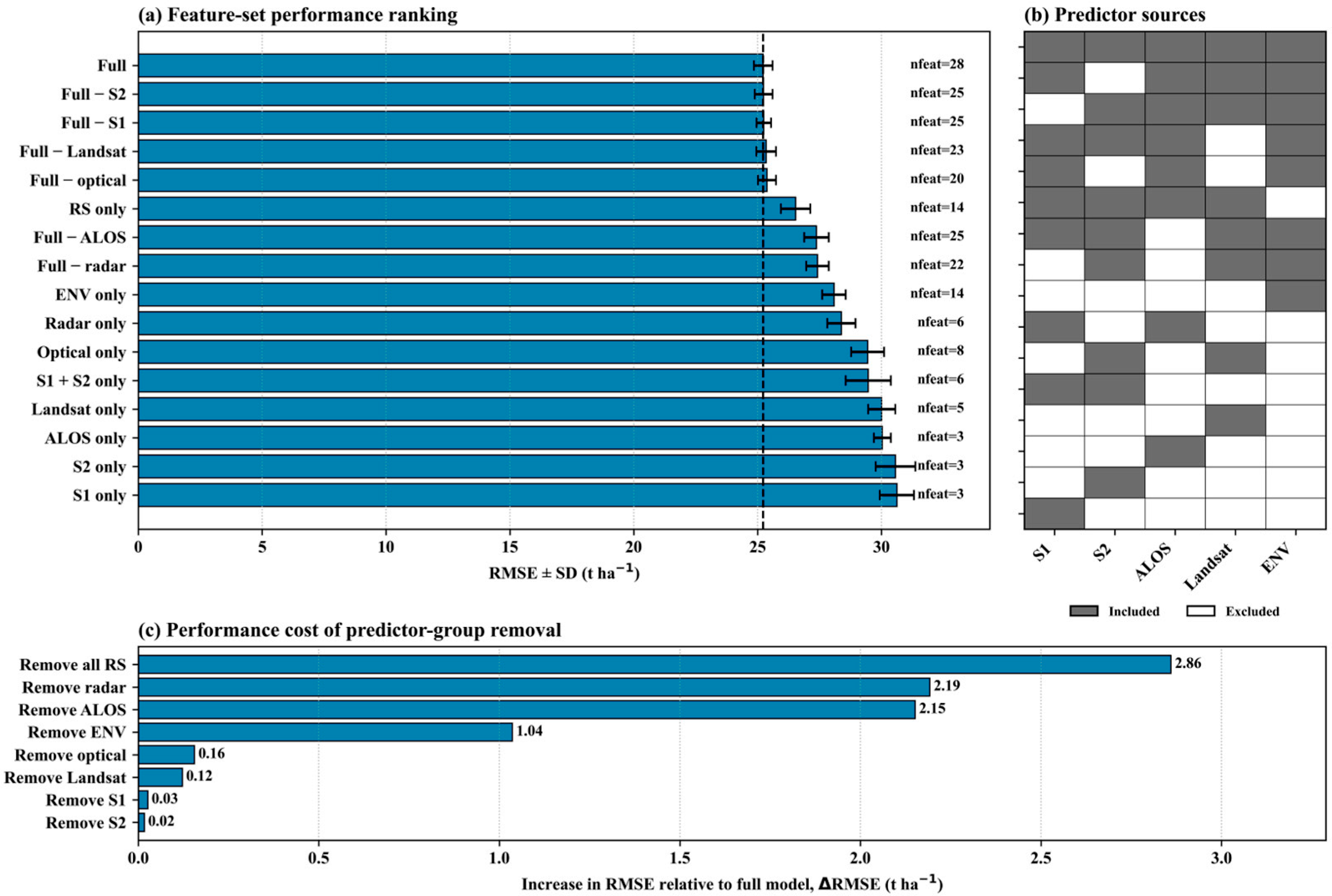
Using the best-performing hyperparameter configuration identified within the baseline search space, feature-set scenarios were compared to assess changes in model performance associated with predictor-set composition. Selected scenarios are summarized in

Table 2. Performance of selected feature-set scenarios using fixed XGBoost hyperparameters. Note: Values are means ± standard deviations across five grouped cross-validation folds. This table reports selected source-removal and source-only scenarios. All scenarios used fixed XGBoost hyperparameters from the baseline-like search-space configuration.

Feature-Set Scenario	Number of Features	Mean RMSE (t ha−1)	Mean MAE (t ha−1)	Mean R2
Full	28	25.22 ± 0.37	20.97 ± 0.41	0.52 ± 0.03
Full minus Sentinel-2	25	25.24 ± 0.36	21.00 ± 0.38	0.51 ± 0.03
Full minus Sentinel-1 C-band SAR	25	25.25 ± 0.29	21.00 ± 0.31	0.49 ± 0.03
Full minus Landsat	23	25.35 ± 0.40	21.11 ± 0.40	0.49 ± 0.03
Full minus environmental	14	26.26 ± 0.51	21.72 ± 0.44	0.44 ± 0.03
Full minus ALOS L-band SAR	25	27.37 ± 0.50	22.51 ± 0.36	0.39 ± 0.01
Full minus radar	22	27.41 ± 0.45	22.53 ± 0.32	0.39 ± 0.01
Environmental only	14	28.08 ± 0.47	23.08 ± 0.35	0.35 ± 0.01
Radar only	6	28.38 ± 0.57	23.13 ± 0.47	0.33 ± 0.04
Optical only	8	29.44 ± 0.67	24.11 ± 0.44	0.28 ± 0.02

using RMSE, MAE, and R^{2 values}. The full multi-source feature set achieved the lowest error, with an RMSE of 25.22 ± 0.37 t ha⁻¹, an MAE of 20.97 ± 0.41 t ha⁻¹, and an R² of 0.52 ± 0.03. Removing Sentinel-2, Sentinel-1, or Landsat resulted in only small increases in RMSE, which reached 25.24 ± 0.36, 25.25 ± 0.29, and 25.35 ± 0.40 t ha⁻¹, respectively.

More pronounced performance losses occurred when environmental/geographic or radar information was removed. Excluding the environmental/geographic predictor group increased RMSE to 26.26 ± 0.51 t ha⁻¹, while removing ALOS L-band SAR or all radar predictors increased RMSE to 27.37 ± 0.50 and 27.41 ± 0.45 t ha⁻¹, respectively. Relative to the full multi-source configuration, the largest RMSE increases followed the removal of all remote-sensing predictors, all radar predictors, or ALOS L-band SAR. By contrast, removing Sentinel-1, Sentinel-2, Landsat, or the complete optical group produced comparatively small changes in model performance.

Source-only configurations performed less accurately than the full multi-source model. Among these configurations, the environmental/geographic-only model achieved the lowest RMSE at 28.08 ± 0.47 t ha⁻¹, followed by the radar-only and optical-only models, which had RMSEs of 28.38 ± 0.57 and 29.44 ± 0.67 t ha⁻¹, respectively. Overall, the full multi-source configuration outperformed all evaluated source-removal and source-only configurations.

3.3. Optimized Model Performance and Robustness Analyses

Among the 303 completed Optuna trials, trial 223 produced the lowest mean grouped-validation RMSE. The optimized model achieved an RMSE of 25.08 ± 0.36 t ha⁻¹, MAE of 20.89 ± 0.39 t ha⁻¹, and R² of 0.53 ± 0.02. Relative RMSE was 36.10 ± 0.52%, while normalized RMSE relative to the observed AGB range was 11.05 ± 0.16%. Compared with the best expanded search-space configuration, the final optimization reduced RMSE by 0.10 t ha⁻¹, indicating only a modest additional improvement in predictive performance.

The optimized configuration used 2600 boosting trees, a learning rate of 0.0148, a maximum tree depth of 4, and a minimum child weight of 5. Row and column subsampling rates were 0.75 and 0.45, respectively. The model used no split-loss reduction or L1 regularization, an L2 regularization value of 2.426, and a maximum histogram bin size of 384. The complete optimized hyperparameter configuration and corresponding search domains are reported in Table A2.

The leakage-sensitivity analysis showed that incorporating feature selection within the grouped cross-validation pipeline had a negligible effect on predictive error. The fold-specific procedure retained 25–29 numeric predictors per fold (mean = 26.2) and yielded an RMSE of 25.19 ± 0.52 t ha⁻¹ and an MAE of 20.96 ± 0.53 t ha⁻¹. Under the otherwise identical fixed-feature baseline, evaluated in the same computing environment and using the same folds, the RMSE and MAE were 25.15 ± 0.45 and 20.92 ± 0.48 t ha⁻¹, respectively. Thus, fold-specific feature selection increased RMSE by only 0.04 t ha⁻¹ and MAE by 0.04 t ha⁻¹, indicating negligible sensitivity of predictive error to the original feature-selection strategy.

Model performance was highly consistent across the three random seeds. Seed-specific RMSE ranged from 25.08 to 25.17 t ha⁻¹, corresponding to a maximum difference of only 0.09 t ha⁻¹, while prediction bias remained between 0.02 and 0.05 t ha⁻¹ (

Table 3. Seed robustness assessment of the optimized XGBoost model. RMSE and MAE are reported as mean ± SD across five grouped cross-validation folds, whereas bias and residual SD were calculated from pooled out-of-fold residuals. The across-seed row reports the mean ± SD across the three seed-level means. All metrics are expressed in t ha⁻¹ and rounded to two decimal places.

Seed	RMSE (t ha−1)	MAE (t ha−1)	Bias (t ha−1)	Residual SD (t ha−1)
42	25.08 ± 0.36	20.89 ± 0.39	0.05	25.09
123	25.14 ± 0.40	20.92 ± 0.43	0.03	25.15
2025	25.17 ± 0.35	20.94 ± 0.35	0.02	25.17
Across-seed mean ± SD	25.13 ± 0.04	20.92 ± 0.03	—	—

). This limited variation shows that the optimized model was not materially sensitive to stochastic differences among training runs.

3.4. Prediction Errors Across Observed AGB Classes

Prediction errors varied substantially across the observed AGB range (

Table 4. Class-specific out-of-fold prediction errors for the optimized XGBoost model. Residuals were calculated as observed minus predicted AGB, with positive values indicating underestimation. Relative RMSE was calculated using the class-specific mean observed AGB. The 95% bootstrap confidence intervals reported for mean residuals were obtained from 5000 within-class resamples.

Observed AGB Class	n	Mean Observed AGB	Mean-Predicted AGB	RMSE	rRMSE (%)	Mean Residual	Bootstrap 95% CI
≤50	1073	31.15	56.19	29.03	93.22	−25.04	−25.92 to −24.16
50–100	2013	74.43	70.32	18.77	25.21	4.11	3.32 to 4.91
100–150	601	115.00	87.00	33.07	28.76	28.00	26.55 to 29.42
>150	38	169.10	127.69	43.89	25.96	41.41	36.55 to 46.01

; Figure 3). The model overestimated AGB in the lowest biomass class (≤50 t ha⁻¹), for which the mean residual was −25.04 t ha⁻¹, RMSE was 29.03 t ha⁻¹, and relative RMSE reached 93.22%. The lowest RMSE occurred for observations between 50 and 100 t ha⁻¹, with an RMSE of 18.77 t ha⁻¹ and a relative RMSE of 25.21%. In contrast, systematic underestimation became increasingly evident at higher observed AGB. For the 100–150 t ha⁻¹ class, the mean residual was −28.00 t ha⁻¹ and RMSE was 33.07 t ha⁻¹. The strongest underestimation occurred in the >150 t ha⁻¹ class, where the mean residual was 41.41 t ha⁻¹ (95% bootstrap CI: 36.55–46.01 t ha⁻¹) and RMSE reached 43.89 t ha⁻¹, although this class contained only 38 observations. The residual plot also showed that most high-biomass observations were located above the zero-residual line. These results indicate a regression-to-the-mean pattern, characterized by overestimation at low biomass and progressively greater underestimation at high biomass.

3.5. North–South Spatial Validation, Longitude Sensitivity, and Applicability-Domain Assessment

The matched north–south spatial-validation analysis produced higher prediction error than the conventional PlotName-grouped assessment. Using the same model inputs, preprocessing procedure, optimized XGBoost hyperparameters, and fitting strategy, the matched five-fold GroupKFold reference yielded an RMSE of 25.20 ± 0.43 t ha⁻¹, whereas five-fold latitudinal-block cross-validation yielded an RMSE of 27.56 ± 2.76 t ha⁻¹. Thus, latitudinal blocking increased mean RMSE by 2.37 t ha⁻¹. The five validation blocks contained approximately 742 unique physical plots each. From the southernmost to the northernmost block, the corresponding RMSE values were 25.76, 26.98, 24.75, 28.51, and 31.80 t ha⁻¹, respectively. Although the prediction error did not increase monotonically across all five blocks, RMSE increased markedly in the two northernmost blocks and reached its highest value in the northernmost holdout. This block contained 742 unique PlotName groups and extended from 48.60° to 51.82°N, compared with the narrower latitudinal ranges represented by the four blocks farther south.

The paired coordinate-sensitivity analysis indicated only limited dependence on explicit longitude. Replacing longitude with the training-fold median increased RMSE from 25.39 to 25.52 t ha⁻¹, corresponding to an increase of 0.12 t ha⁻¹ (0.49%), and increased MAE from 21.13 to 21.23 t ha⁻¹. Pooled R² decreased by only 0.006. Thus, longitude provided a modest predictive contribution but did not dominate the model’s grouped cross-validated performance.

The reference plots spanned 46.37–51.82°N, whereas the wildfire sample points extended from 46.55 to 58.61°N. Overall, 52.23% of wildfire sample points occurred within the latitudinal range represented by the reference plots, while 47.77% were located north of the observed reference-data range. Among the 9854 wildfire points with complete data for all 14 final environmental/geographic predictors, 60.64% fell outside the univariate training range for at least one predictor, whereas 39.36% fell within the training ranges of all predictors (

Table A5. Univariate applicability-domain assessment of the final environmental/geographic predictors at wildfire sample points.

Predictor	Training Range	Valid Wildfire Points (n)	Below Range (%)	Within Range (%)	Above Range (%)
Growing-season AT10 anomaly (degree-days)	−235.96 to 205.97	9937	0.00	98.57	1.43
Longitude (decimal degrees)	−94.73 to −68.47	9937	6.58	82.49	10.93
Annual precipitation anomaly (mm)	−146.31 to 281.48	9937	3.33	95.69	0.98
Sand content, 0–5 cm	215.60 to 699.59	9854	0.01	97.28	2.71
Clay content, 0–5 cm	71.55 to 365.69	9854	0.68	99.31	0.01
Silt content, 0–5 cm	198.47 to 494.57	9854	2.66	97.23	0.11
Total soil nitrogen, 0–5 cm	2716.85 to 12,073.92	9854	0.31	99.69	0.00
Baseline annual mean temperature (°C)	−1.92 to 5.63	9937	17.57	82.43	0.00
Elevation (m)	50.17 to 1090.96	9937	1.57	98.43	0.00
Annual mean temperature anomaly (°C)	−1.27 to 1.53	9937	9.27	85.30	5.43
Baseline annual precipitation (mm)	675.20 to 1442.42	9937	21.38	78.62	0.00
Slope (degrees)	0.24 to 32.48	9937	0.39	99.42	0.19
Growing-season precipitation anomaly (mm)	−169.28 to 121.19	9937	0.41	96.89	2.70
Annual mean temperature (°C)	−0.52 to 6.31	9937	40.42	59.58	0.00

). On average, each wildfire point was outside the training range for 1.29 predictors. At the individual-predictor level, coverage was lowest for annual mean temperature (59.58%), baseline annual precipitation (78.62%), baseline annual mean temperature (82.43%), and longitude (82.49%), while coverage for the remaining predictors ranged from 85.30% to 99.69%.

3.6. Annual Wildfire-Related Potential AGB Exposure Estimation, Sampling Uncertainty, and Sensitivity Analyses

Application of the optimized multi-source XGBoost model to the land-cover-stratified wildfire sample yielded a cumulative potential AGB exposure of 269.20 Mt over 6.66 Mha of effective burned area during 2018–2024, corresponding to an area-weighted mean exposure intensity of 40.43 t ha⁻¹. The polygon-level bootstrap distribution was closely centered on the baseline estimate, with a mean of 269.18 Mt, a median of 269.20 Mt, a 95% finite-point sampling bootstrap interval of 254.19–284.06 Mt, and a coefficient of variation of 2.86% (

Table 5. Annual and cumulative baseline potential AGB exposure under the complete-loss assumption (λ = 1). Bracketed values are 95% finite-point sampling bootstrap intervals derived from 5000 polygon-level resamples; they do not include AGB model, spatial extrapolation, land cover, or fire perimeter uncertainty.

Year	Baseline Potential Exposure, λ = 1 (Mt) [95% Bootstrap Sampling Interval]
2018	7.84 [7.18 to 8.54]
2019	5.62 [4.56 to 6.78]
2020	1.76 [1.40 to 2.20]
2021	33.03 [30.32 to 35.83]
2022	1.38 [1.27 to 1.48]
2023	206.44 [191.89 to 220.93]
2024	13.12 [12.24 to 14.05]
2018–2024	269.20 [254.19 to 284.06]

). Relative sampling variability was greater in 2019 and 2020, with coefficients of variation of 10.11% and 11.87%, respectively, but remained below 4.5% in most other years. The 2023 estimate was 206.44 Mt, with a 95% sampling interval of 191.89–220.93 Mt, and remained substantially higher than all other annual estimates. Thus, the dominance of the 2023 fire season was robust to finite-point sampling variability.

Under the alternative biomass-loss fractions, cumulative scenario estimates ranged from 53.84 Mt at $f=0.2$ to 134.60 Mt at $f=0.5$, compared with the complete-loss baseline of 269.20 Mt. Corresponding exposure intensities ranged from 8.09 to 20.22 t ha⁻¹ (

Table A6. Sensitivity of cumulative wildfire-related potential AGB exposure to alternative hypothetical biomass loss fractions during 2018–2024.

Biomass-Loss Fraction, λ	Cumulative Scenario Estimate (Mt)	Exposure Intensity (t ha−1)	Relative to Baseline (%)
0.20	53.84	8.09	20
0.30	80.76	12.13	30
0.40	107.68	16.17	40
0.50	134.60	20.22	50
1.00	269.20	40.43	100

). The scenario estimates scaled linearly with the assumed biomass-loss fraction and represented sensitivity bounds rather than measured biomass consumption.

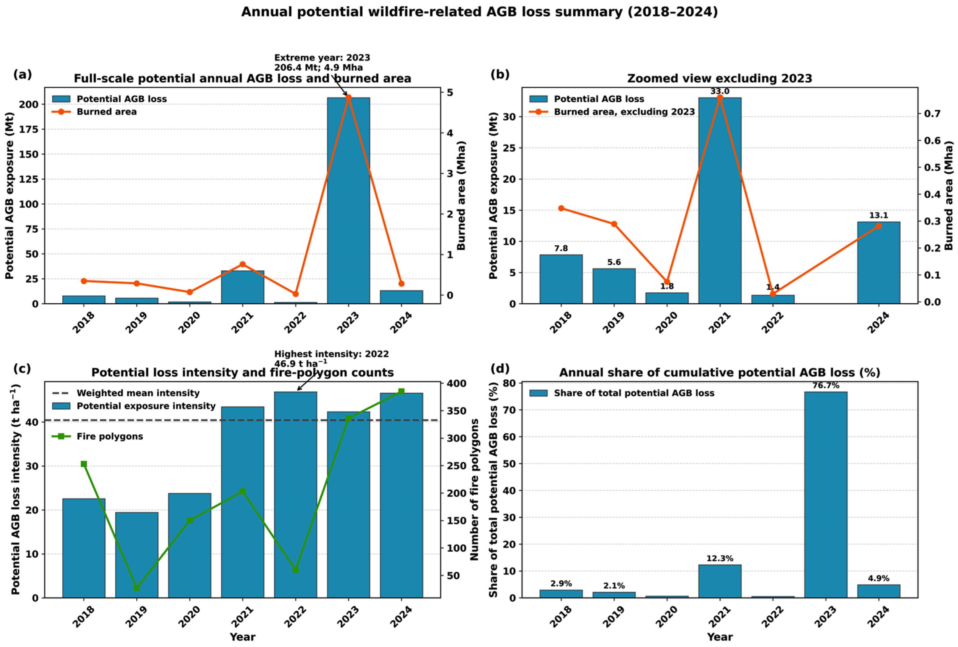
Annual wildfire-related potential AGB exposure varied strongly among years and was dominated by the exceptional 2023 fire season (Figure 4a). In 2023, potential exposure reached 206.44 Mt across 4.88 Mha of effective burned area, representing 76.7% of cumulative exposure and 73.2% of cumulative effective burned area during 2018–2024 (Figure 4d). Excluding 2023, the remaining six years contributed a cumulative 62.76 Mt, equivalent to 23.3% of the seven-year total. Among these non-extreme years, the greatest annual potential exposure occurred in 2021, followed by 2024 and 2018 (Figure 4b). Thus, substantial interannual variation remained evident even when the extreme 2023 season was excluded.

Potential AGB loss intensity followed a different annual pattern than total potential AGB loss (Figure 4c). The highest loss intensity occurred in 2022 (46.86 t ha⁻¹), despite the relatively low total potential AGB loss in that year. The year 2024 also showed high loss intensity and had the greatest number of mapped fire polygons (385). Burned area and total potential AGB loss were almost perfectly correlated (r = 0.99), whereas the association between burned area and loss intensity was weaker (r = 0.28). Accordingly, years with greater burned area consistently had greater total estimated AGB loss, but larger fire years did not necessarily exhibit greater loss per unit area. The contrast among total potential AGB loss, burned area, and loss intensity is visible across the panels of Figure 4.

The 2023 sensitivity analyses indicated that alternative land-cover eligibility and within-perimeter burn correction affected the magnitude of the baseline estimate but did not alter the identification of 2023 as the dominant fire year (Table A4). The pre-fire Dynamic World composite provided valid land-cover information for 99.93% of the assessed polygon raster and produced an eligible-area estimate that was 1.41% greater than the corresponding NALCMS eligible area. Applying this area ratio increased the 2023 potential exposure from 206.44 to 209.36 Mt. The mean-predicted AGB at Dynamic World-eligible existing points was only 0.47% greater than the mean across all valid existing points; including this intensity adjustment produced an estimate of 210.33 Mt, representing a 1.88% increase relative to the NALCMS-based baseline. The dNBR analysis provided valid observations for 99.20% of the polygon raster. Thresholds of $dNBR \ge 0.05, \ge 0.10,$ and $\ge 0.20$ retained 98.14%, 96.00%, and 88.73% of the valid area, respectively, yielding area-corrected 2023 exposure estimates of 202.60, 198.19, and 183.18 Mt. These correspond to reductions of 1.86%, 4.00%, and 11.27% relative to the uncorrected estimate. Thus, the 2023 estimate was comparatively insensitive to the alternative pre-fire land-cover product and the less restrictive dNBR criteria, whereas the strictest spectral-change threshold produced a larger, but bounded, reduction.

4. Discussion

4.1. Complementarity Among Optical, SAR, and Environmental/Geographic Predictors

The feature-set comparison showed that AGB estimation across the boreal forests of Quebec and Ontario benefited from integrating multiple predictor sources. The full multi-source model achieved the lowest cross-validated error among all evaluated configurations (Figure 5a). The ablation results further suggest that optical, SAR, environmental, and geographic predictors capture complementary aspects of biomass variability, including canopy spectral condition, woody structure, moisture-related scattering, site conditions, and broad geographic gradients.

Among the remote-sensing sources, the radar contribution was primarily associated with ALOS L-band SAR. Removing all radar predictors or ALOS alone produced two of the largest increases in RMSE, whereas removing Sentinel-1 caused only a minor change (Figure 5c). This pattern is physically plausible because L-band observations are generally more responsive to woody components and canopy structure, whereas C-band backscatter is more influenced by upper-canopy properties and vegetation moisture, and may saturate at lower biomass levels. This pattern is consistent with multisensor AGB studies showing that L-band observations provide useful information on woody components and forest structure [23,29]. Thus, the limited effect of removing Sentinel-1 should not be interpreted as evidence that radar information was unimportant; rather, ALOS provided substantially more independent information in this boreal context.

Environmental/geographic predictors also contributed meaningfully to model performance. Removing this predictor group increased RMSE by 1.04 t ha⁻¹, whereas the environmental/geographic-only configuration outperformed several sensor-only models but remained less accurate than the full model (Figure 5a–c). These predictors likely captured broad gradients in climate, terrain, soil properties, and geographic position that were not fully represented by remote-sensing data alone. This finding agrees with previous work showing that environmental predictors can improve regional boreal AGB estimation when combined with optical observations [5].

Optical predictors showed a smaller independent contribution after integration with radar and environmental information. Removing Sentinel-2, Landsat, or the complete optical group produced relatively small increases in RMSE (Figure 5c), suggesting partial overlap with information retained in the other predictor groups. Nevertheless, its red-edge, near-infrared, shortwave-infrared, greenness, moisture, and disturbance-sensitive variables remain biophysically relevant for characterizing canopy condition and vegetation density [17,18,21,34]. Overall, the full model outperformed all reduced-source and source-only configurations, with the strongest independent contributions associated with ALOS L-band SAR and environmental/geographic information, while optical predictors provided additional complementary information across the heterogeneous boreal study region.

4.2. Model Reliability and Comparison with Previous AGB Studies

The reliability of the final AGB estimates was supported by the combined use of product-wise feature selection, grouped cross-validation, and robustness testing. Feature selection reduced redundancy within the initially broad predictor set while retaining information from optical, SAR, environmental, and geographical sources. Similar screening approaches have been used in previous AGB studies to improve model parsimony and reduce the influence of correlated predictors [18,21,34,36]. In contrast, expanding the hyperparameter search space and applying final Optuna optimization produced only modest improvements in predictive accuracy. The limited variation among random-seed runs further indicated that the final model performance was not strongly affected by stochastic differences in model training. Together, these results suggest that predictor construction, source integration, and leakage-aware validation were more influential for model reliability than increasing optimization complexity alone.

The optimized multi-source model achieved an RMSE of 25.08 ± 0.36 t ha⁻¹, an MAE of 20.89 ± 0.39 t ha⁻¹, and an R² of 0.53 ± 0.02 under five-fold grouped cross-validation. This performance should be interpreted in the context of the large study area, heterogeneous forest conditions, multi-year plot observations, and broad AGB range represented in the reference dataset. Direct numerical comparison with previous studies remains difficult because reported accuracies depend on biome, forest structure, plot size, reference data, biomass range, sensor configuration, and validation design. Studies conducted in smaller or more homogeneous ecological domains, or using random train–test splits, may report higher coefficients of determination without necessarily demonstrating equivalent transferability to heterogeneous regional forest conditions.

The class-specific diagnostics revealed an important limitation that was obscured by the near-zero pooled mean residual. Predictions showed regression toward the mean, with AGB overestimated for observations in the lower biomass range and increasingly underestimated for observations above 100 t ha⁻¹. This pattern may reflect the limited representation of high-biomass stands, as only 38 observations exceeded 150 t ha⁻¹, combined with reduced sensitivity of optical and SAR predictors in dense canopies and the absence of direct measurements of canopy height and vertical structure [17,20,24]. Consequently, potential AGB exposure may be underestimated where fires intersect high-biomass stands and overestimated in low-biomass landscapes. Opposing class-specific errors may partially cancel out in pooled metrics; therefore, a small overall mean residual should not be interpreted as uniformly unbiased performance across the AGB range.

The present results are most comparable with studies using field-based reference data or relatively conservative validation strategies. For example, Guerra-Hernández et al. [29] reported an R² of 0.63 and an RMSE of 11.10 Mg ha⁻¹ when evaluating wall-to-wall biomass predictions against ICESat-2-derived reference estimates, whereas performance against independent field plots decreased to an R² of 0.43 and an RMSE of 25.88 Mg ha⁻¹. The latter error magnitude is close to that obtained in the present study and illustrates the greater difficulty of predicting plot-level forest AGB across structurally heterogeneous landscapes. Moghimi et al. [21] similarly reported moderate R² values of approximately 0.5–0.6 for Sentinel-1 and Sentinel-2 forest AGB models, depending on the region and predictor configuration. By comparison, higher values reported in some multi-source studies, such as [18,34], were obtained under different vegetation conditions, biomass ranges, and validation designs, and are therefore not directly transferable to the eastern Canadian boreal context.

An important distinction of the present study is that repeated observations from the same field plot were retained within the same cross-validation fold. This grouping reduced plot-level information leakage and provided a more conservative assessment of model generalization than random record-level partitioning. The resulting moderate R², consistent RMSE across folds and random seeds, and improved performance from multi-source integration indicate that the model provides a sufficiently stable basis for regional application. The purpose of the modeling framework was not solely to maximize plot-level predictive accuracy, but to generate reproducible estimates of potential pre-fire AGB that could be linked with wildfire perimeters and land-cover-stratified sampling across Quebec and Ontario.

4.3. Wildfire Extent, Potential AGB Loss Intensity, and Potential AGB Loss

Interannual variation in total potential AGB loss was dominated by variation in effective burned area. This relationship is partly inherent in the calculation, which combines predicted pre-fire AGB density with the burned extent. However, the magnitude of variation in fire extent was sufficient to outweigh annual differences in the mean estimated biomass density of burned landscapes. The exceptional 2023 fire season illustrates this scale effect: its extensive burned area dominated the 2018–2024 record, indicating that regional estimates of wildfire-related biomass exposure can be strongly influenced by a single extreme fire year.

Potential AGB loss intensity provided complementary information by expressing potential AGB loss per unit of effective burned area. Although 2023 produced by far the greatest total potential AGB loss, it did not have the highest loss intensity. In contrast, 2022 had relatively low burned area and total potential AGB loss but the highest loss intensity, indicating that burning in that year was concentrated in landscapes with comparatively high estimated pre-fire AGB density. Large fire years therefore do not necessarily affect the highest-biomass landscapes on average, while smaller fire years may have high loss intensity when burning occurs in biomass-rich stands.

One possible explanation is that years with extensive fires encompass a broader range of vegetation and biomass conditions, thereby reducing mean biomass exposure per unit burned area. However, annual differences in the land-cover composition of burned areas were not evaluated directly, so this explanation remains a hypothesis rather than a demonstrated mechanism. Taken together, effective burned area, total potential AGB loss, and loss intensity provide a more complete description of wildfire-related biomass exposure than any of these measures alone.

These findings are consistent with previous studies showing that disturbance-related biomass dynamics cannot be characterized from disturbance extent alone. Pelletier et al. [7] demonstrated the value of integrating optical time series with AGB information to characterize biomass dynamics across Canadian forests, whereas Clark et al. [14] showed that post-fire structural change varied with pre-fire forest structure. The present results similarly indicate that spatially explicit pre-fire AGB estimates provide information beyond burned-area mapping alone. Wildfire assessments should therefore distinguish among three related but non-equivalent quantities: effective burned area, which describes the extent of eligible land-cover classes within mapped fire polygons; total potential AGB exposure, which represents the estimated pre-fire biomass stock potentially affected under the complete-loss assumption; and exposure intensity, which represents mean potential AGB exposure per hectare of effective burned area.

4.4. Limitations, Uncertainty, and Future Research Directions

Several sources of uncertainty should be considered when interpreting the plot-level AGB estimates and their regional application. The reference data inherited uncertainties associated with field measurements, allometric biomass estimation, plot geolocation, plot size, and temporal alignment between inventory observations and remote sensing predictors [6]. A more consequential limitation was the uneven spatial distribution of the reference plots, which were concentrated primarily in the southern portion of the study area, whereas many wildfire polygons occurred farther north. The matched latitudinal-block analysis provided a structured sensitivity assessment of this limitation: mean RMSE increased from 25.20 ± 0.43 t ha⁻¹ under PlotName GroupKFold to 27.56 ± 2.76 t ha⁻¹ under north–south blocking and reached 31.80 t ha⁻¹ in the northernmost holdout. The two northernmost blocks produced the highest errors, indicating reduced northward geographic transferability. Consistent with this result, 47.77% of wildfire sample points were located north of the reference-plot latitudinal range, and 60.64% of complete-case wildfire points fell outside the univariate training range for at least one final environmental/geographic predictor. Extrapolation was most evident for annual mean temperature and baseline climatic conditions, reflecting the colder and, in some locations, drier environments of northern burned landscapes. Nevertheless, most individual predictors showed substantial overlap between the reference and wildfire datasets, and wildfire points were outside the training range for only 1.29 predictors on average. These findings do not imply that predictions outside a univariate range were invalid; rather, they identify locations where predictions involved greater environmental extrapolation and require more cautious interpretation. Further work should prioritize denser field sampling and independent validation in northern landscapes, two-dimensional spatial blocking, and structural observations from airborne laser scanning, GEDI, ICESat-2, or forest inventories [14,24,29,45].

The wildfire-related estimates represent potential AGB loss rather than direct measurements of combustion, carbon emissions, or observed post-fire mortality. Actual biomass loss depends on burn severity, combustion completeness, fuel moisture, tree mortality, residual live biomass, snag persistence, decomposition, and post-fire recovery [14,15,16]. Additional uncertainty arises from fire-perimeter delineation, unburned islands, within-polygon variation in burn severity, and the use of a fixed land-cover product that may not fully represent annual disturbance, recovery, or classification changes during 2018–2024. These factors can affect both eligible burned area and potential exposure intensity, particularly where fire polygons contain mixtures of forest, wetland, shrubland, sparse vegetation, and non-vegetated surfaces [7]. Future work should integrate annual land cover, burn-severity metrics, and explicit biomass-consumption parameters, and should formally propagate uncertainty from AGB prediction, land-cover classification, fire-perimeter delineation, and biomass-loss aggregation [56,57].

5. Conclusions

This study developed a multi-source remote-sensing framework for estimating plot-level AGB and translating these estimates into annual wildfire-related potential AGB loss across the boreal forests of Quebec and Ontario during 2018–2024. By combining field-based AGB observations with C-band SAR, Sentinel-2, L-band SAR, Landsat, environmental, and geographic predictors, the framework provides a reproducible basis for linking pre-fire biomass conditions with mapped wildfire perimeters.

The main contribution of this study is that it moves wildfire impact assessment beyond burned-area accounting alone. The results show that annual total potential AGB exposure largely reflects the spatial extent of burning, particularly during the extreme 2023 fire season. However, potential loss intensity followed a different annual pattern, indicating that biomass exposure per unit burned area provides additional information that cannot be inferred from fire extent alone. This distinction is important for boreal carbon monitoring.

Overall, the findings demonstrate that integrating spatially explicit pre-fire AGB estimates with wildfire polygons can improve interpretation of fire impacts by separating the effects of burned area from the effects of biomass exposure. The estimates should be interpreted as potential wildfire-related AGB loss rather than direct carbon emissions or combustion completeness. Future work should strengthen this framework by incorporating LiDAR or GEDI/ICESat-2 structural information, improving reference-data coverage in northern burned landscapes, integrating burn-severity and combustion parameters, and propagating uncertainty from AGB prediction, land-cover classification, and fire-perimeter delineation into final biomass-loss estimates.

References

1. Brandt, J.P. The Extent of the North American Boreal Zone. Environ. Rev. 2009, 17, 101–161. [Google Scholar] [CrossRef] [Scilit]
2. Zhang, Y.; Liang, S.; Yang, L. A Review of Regional and Global Gridded Forest Biomass Datasets. Remote Sens. 2019, 11, 2744. [Google Scholar] [CrossRef] [Scilit]
3. Brandt, J.P.; Flannigan, M.D.; Maynard, D.G.; Thompson, I.D.; Volney, W.J.A. An Introduction to Canada’s Boreal Zone: Ecosystem Processes, Health, Sustainability, and Environmental Issues1. Environ. Rev. 2013, 21, 207–226. [Google Scholar] [CrossRef] [Scilit]
4. Guindon, L.; Manka, F.; Correia, D.L.P.; Villemaire, P.; Smiley, B.; Bernier, P.; Gauthier, S.; Beaudoin, A.; Boucher, J.; Boulanger, Y. A New Approach for Spatializing the Canadian National Forest Inventory (SCANFI) Using Landsat Dense Time Series. Can. J. For. Res. 2024, 54, 793–815. [Google Scholar] [CrossRef] [Scilit]
5. Liu, P.; Ren, C.; Yang, X.; Wang, Z.; Jia, M.; Zhao, C.; Yu, W.; Ren, H. Combining Sentinel-2 and Diverse Environmental Data Largely Improved Aboveground Biomass Estimation in China’s Boreal Forests. Sci. Rep. 2024, 14, 27528. [Google Scholar] [CrossRef] [Scilit] [PubMed]
6. Mahmoudi Meimand, H.; Chen, J.; Kneeshaw, D.; Peng, C. Measurement-Driven Estimates of Above-Ground Biomass Change in the Eastern Canadian Boreal Forests from Permanent Sample Plots and Landsat Time Series. Forests 2026, 17, 575. [Google Scholar] [CrossRef] [Scilit]
7. Pelletier, F.; Cardille, J.A.; Wulder, M.A.; White, J.C.; Hermosilla, T. Inter- and Intra-Year Forest Change Detection and Monitoring of Aboveground Biomass Dynamics Using Sentinel-2 and Landsat. Remote Sens. Environ. 2024, 301, 113931. [Google Scholar] [CrossRef] [Scilit]
8. Boulanger, Y.; Arseneault, D.; Claude Bélisle, A.; Bergeron, Y.; Boucher, Y.; Danneyrolles, V.; Erni, S.; Gachon, P.; Grant, E.; Grondin, P.; et al. The 2023 Wildfire Season in Québec: An Overview of Extreme Conditions, Impacts, Lessons Learned, and Considerations for the Future. Can. J. For. Res. 2025, 55, 1–21. [Google Scholar] [CrossRef] [Scilit]
9. Pelletier, F.; Cardille, J.A.; Wulder, M.A.; White, J.C.; Hermosilla, T. Revisiting the 2023 Wildfire Season in Canada. Sci. Remote Sens. 2024, 10, 100145. [Google Scholar] [CrossRef] [Scilit]
10. Byrne, B.; Liu, J.; Bowman, K.W.; Pascolini-Campbell, M.; Chatterjee, A.; Pandey, S.; Miyazaki, K.; van der Werf, G.R.; Wunch, D.; Wennberg, P.O.; et al. Carbon Emissions from the 2023 Canadian Wildfires. Nature 2024, 633, 835–839. [Google Scholar] [CrossRef] [Scilit] [PubMed]
11. Meimand, H.M.; Chen, J.; Kneeshaw, D.; Bakhtyari, M.; Peng, C. Burned Area Detection in the Eastern Canadian Boreal Forest Using a Multi-Layer Perceptron and MODIS-Derived Features. Remote Sens. 2025, 17, 2162. [Google Scholar] [CrossRef] [Scilit]
12. Zhang, P.; Hu, X.; Ban, Y.; Nascetti, A.; Gong, M. Assessing Sentinel-2, Sentinel-1, and ALOS-2 PALSAR-2 Data for Large-Scale Wildfire-Burned Area Mapping: Insights from the 2017–2019 Canada Wildfires. Remote Sens. 2024, 16, 556. [Google Scholar] [CrossRef] [Scilit]
13. Bottani, M.; Ferro-Famil, L.; Poccard-Chapuis, R.; Polidori, L. Continuous Monitoring of Fire-Induced Forest Loss Using Sentinel-1 SAR Time Series and a Bayesian Method: A Case Study in Paragominas, Brazil. Remote Sens. 2025, 17, 2822. [Google Scholar] [CrossRef] [Scilit]
14. Clark, M.L.; Hakkenberg, C.R.; Bailey, T.; Burns, P.; Goetz, S.J. Changes in GEDI-Based Measures of Forest Structure after Large California Wildfires Relative to Pre-Fire Conditions. Remote Sens. Environ. 2025, 323, 114718. [Google Scholar] [CrossRef] [Scilit]
15. Cui, L.; Xu, X.; Chen, S. Estimating Biomass Consumption and Carbon Emissions by Integrating GEDI, Sentinel-1, and Sentinel-2 Data. Ecol. Indic. 2025, 178, 113889. [Google Scholar] [CrossRef] [Scilit]
16. Liu, M.; Popescu, S. Estimation of Biomass Burning Emissions by Integrating ICESat-2, Landsat 8, and Sentinel-1 Data. Remote Sens. Environ. 2022, 280, 113172. [Google Scholar] [CrossRef] [Scilit]
17. Moradi, F.; Darvishsefat, A.A.; Pourrahmati, M.R.; Deljouei, A.; Borz, S.A. Estimating Aboveground Biomass in Dense Hyrcanian Forests by the Use of Sentinel-2 Data. Forests 2022, 13, 104. [Google Scholar] [CrossRef] [Scilit]
18. Naik, P.; Dalponte, M.; Bruzzone, L. Automated Machine Learning Driven Stacked Ensemble Modeling for Forest Aboveground Biomass Prediction Using Multitemporal Sentinel-2 Data. IEEE J. Sel. Top. Appl. Earth Obs. Remote Sens. 2023, 16, 3442–3454. [Google Scholar] [CrossRef] [Scilit]
19. Poudel, A.; Shrestha, H.L.; Mahat, N.; Sharma, G.; Aryal, S.; Kalakheti, R.; Lamsal, B. Modeling and Mapping of Aboveground Biomass and Carbon Stock Using Sentinel-2 Imagery in Chure Region, Nepal. Int. J. For. Res. 2023, 2023, 5553957. [Google Scholar] [CrossRef] [Scilit]
20. Wang, J.; Xiang, C.; Liang, A. Estimation of Forest Aboveground Biomass in China Based on GEDI and Sentinel-2 Data: Quantitative Analysis of Optical Remote Sensing Saturation Effect and Terrain Compensation Mechanisms. Remote Sens. 2025, 17, 3437. [Google Scholar] [CrossRef] [Scilit]
21. Moghimi, A.; Tavakoli Darestani, A.; Mostofi, N.; Fathi, M.; Amani, M. Improving Forest Above-Ground Biomass Estimation Using Genetic-Based Feature Selection from Sentinel-1 and Sentinel-2 Data (Case Study of the Noor Forest Area in Iran). Kuwait J. Sci. 2024, 51, 100159. [Google Scholar] [CrossRef] [Scilit]
22. Nuthammachot, N.; Askar, A.; Stratoulias, D.; Wicaksono, P. Combined Use of Sentinel-1 and Sentinel-2 Data for Improving above-Ground Biomass Estimation. Geocarto Int. 2022, 37, 366–376. [Google Scholar] [CrossRef] [Scilit]
23. Wang, C.; Zhang, W.; Ji, Y.; Marino, A.; Li, C.; Wang, L.; Zhao, H.; Wang, M. Estimation of Aboveground Biomass for Different Forest Types Using Data from Sentinel-1, Sentinel-2, ALOS PALSAR-2, and GEDI. Forests 2024, 15, 215. [Google Scholar] [CrossRef] [Scilit]
24. Chen, L.; Ren, C.; Bao, G.; Zhang, B.; Wang, Z.; Liu, M.; Man, W.; Liu, J. Improved Object-Based Estimation of Forest Aboveground Biomass by Integrating LiDAR Data from GEDI and ICESat-2 with Multi-Sensor Images in a Heterogeneous Mountainous Region. Remote Sens. 2022, 14, 2743. [Google Scholar] [CrossRef] [Scilit]
25. Nandy, S.; Srinet, R.; Padalia, H. Mapping Forest Height and Aboveground Biomass by Integrating ICESat-2, Sentinel-1 and Sentinel-2 Data Using Random Forest Algorithm in Northwest Himalayan Foothills of India. Geophys. Res. Lett. 2021, 48, e2021GL093799. [Google Scholar] [CrossRef] [Scilit]
26. Tamiminia, H.; Salehi, B.; Mahdianpari, M.; Beier, C.M.; Johnson, L.; Phoenix, D.B. A Comparison of Random Forest and Light Gradient Boosting Machine for Forest Above-Ground Biomass Estimation Using a Combination of Landsat, Alos Palsar, and Airborne LiDAR Data. In Proceedings of the International Archives of the Photogrammetry, Remote Sensing and Spatial Information Sciences—ISPRS Archives; Copernicus GmbH: Göttingen, Germany, 2021; Volume 44. [Google Scholar]
27. Tang, Z.; Xia, X.; Huang, Y.; Lu, Y.; Guo, Z. Estimation of National Forest Aboveground Biomass from Multi-Source Remotely Sensed Dataset with Machine Learning Algorithms in China. Remote Sens. 2022, 14, 5487. [Google Scholar] [CrossRef] [Scilit]
28. Fang, G.; Yu, H.; Fang, L.; Zheng, X. Synergistic Use of Sentinel-1 and Sentinel-2 Based on Different Preprocessing for Predicting Forest Aboveground Biomass. Forests 2023, 14, 1615. [Google Scholar] [CrossRef] [Scilit]
29. Guerra-Hernández, J.; Narine, L.L.; Pascual, A.; Gonzalez-Ferreiro, E.; Botequim, B.; Malambo, L.; Neuenschwander, A.; Popescu, S.C.; Godinho, S. Aboveground Biomass Mapping by Integrating ICESat-2, SENTINEL-1, SENTINEL-2, ALOS2/PALSAR2, and Topographic Information in Mediterranean Forests. GIsci. Remote Sens. 2022, 59, 1509–1533. [Google Scholar] [CrossRef] [Scilit]
30. Melitha, G.S.; Kashaigili, J.J.; Mugasha, W.A. Integrating UAV, Sentinel-2, and ALOS PALSAR-2 Data for Improving above-Ground Biomass Estimation in Miombo Woodlands Using Machine Learning Algorithms. Int. J. Remote Sens. 2025, 46, 4796–4831. [Google Scholar] [CrossRef] [Scilit]
31. Guo, Y.; Li, Z.; Zhang, X.; Chen, E.X.; Bai, L.; Tian, X.; He, Q.; Feng, Q.; Li, W. Optimal Support Vector Machines for Forest Above-Ground Biomass Estimation from Multisource Remote Sensing Data. In Proceedings of the International Geoscience and Remote Sensing Symposium (IGARSS), Munich, Germany, 22–27 July 2012. [Google Scholar]
32. Li, Y.; Li, M.; Li, C.; Liu, Z. Forest Aboveground Biomass Estimation Using Landsat 8 and Sentinel-1A Data with Machine Learning Algorithms. Sci. Rep. 2020, 10, 9952. [Google Scholar] [CrossRef] [Scilit] [PubMed]
33. Singh, C.; Karan, S.K.; Sardar, P.; Samadder, S.R. Remote Sensing-Based Biomass Estimation of Dry Deciduous Tropical Forest Using Machine Learning and Ensemble Analysis. J. Environ. Manag. 2022, 308, 114639. [Google Scholar] [CrossRef] [Scilit] [PubMed]
34. Xu, Y.; Qin, Y.; Li, B.; Li, J. Estimating Vegetation Aboveground Biomass in Yellow River Delta Coastal Wetlands Using Sentinel-1, Sentinel-2 and Landsat-8 Imagery. Ecol. Inform. 2025, 87, 103096. [Google Scholar] [CrossRef] [Scilit]
35. Li, C.; Zhou, L.; Xu, W. Estimating Aboveground Biomass Using Sentinel-2 Msi Data and Ensemble Algorithms for Grassland in the Shengjin Lake Wetland, China. Remote Sens. 2021, 13, 1595. [Google Scholar] [CrossRef] [Scilit]
36. Wu, N.; Crusiol, L.G.T.; Liu, G.; Wuyun, D.; Han, G. Comparing the Performance of Machine Learning Algorithms for Estimating Aboveground Biomass in Typical Steppe of Northern China Using Sentinel Imageries. Ecol. Indic. 2023, 154, 110723. [Google Scholar] [CrossRef] [Scilit]
37. Molina, E.; Valeria, O.; Martin, M.; Montoro Girona, M.; Ramirez, J.A. Long-Term Impacts of Forest Management Practices under Climate Change on Structure, Composition, and Fragmentation of the Canadian Boreal Landscape. Forests 2022, 13, 1292. [Google Scholar] [CrossRef] [Scilit]
38. Roy, D.P.; Wulder, M.A.; Loveland, T.R.; C.E., W.; Allen, R.G.; Anderson, M.C.; Helder, D.; Irons, J.R.; Johnson, D.M.; Kennedy, R.; et al. Landsat-8: Science and Product Vision for Terrestrial Global Change Research. Remote Sens. Environ. 2014, 145, 154–172. [Google Scholar] [CrossRef] [Scilit]
39. Trevisani, S.; Skrypitsyna, T.N.; Florinsky, I.V. Global Digital Elevation Models for Terrain Morphology Analysis in Mountain Environments: Insights on Copernicus GLO-30 and ALOS AW3D30 for a Large Alpine Area. Environ. Earth Sci. 2023, 82, 198. [Google Scholar] [CrossRef] [Scilit]
40. Poggio, L.; De Sousa, L.M.; Batjes, N.H.; Heuvelink, G.B.M.; Kempen, B.; Ribeiro, E.; Rossiter, D. SoilGrids 2.0: Producing Soil Information for the Globe with Quantified Spatial Uncertainty. Soil 2021, 7, 217–240. [Google Scholar] [CrossRef] [Scilit]
41. Abatzoglou, J.T.; Dobrowski, S.Z.; Parks, S.A.; Hegewisch, K.C. TerraClimate, a High-Resolution Global Dataset of Monthly Climate and Climatic Water Balance from 1958–2015. Sci. Data 2018, 5, 170191. [Google Scholar] [CrossRef] [Scilit] [PubMed]
42. Natural Resources Canada. 2020 Land Cover of Canada; Natural Resources Canada: Ottawa, ON, Canada, 2022.
43. Chen, T.; Guestrin, C. XGBoost: A Scalable Tree Boosting System. In Proceedings of the ACM SIGKDD International Conference on Knowledge Discovery and Data Mining, San Francisco, CA, USA, 13–17 August 2016. [Google Scholar]
44. Pedregosa, F.; Varoquaux, G.; Gramfort, A.; Michel, V.; Thirion, B.; Grisel, O.; Blondel, M.; Prettenhofer, P.; Weiss, R.; Dubourg, V.; et al. Scikit-Learn: Machine Learning in Python. J. Mach. Learn. Res. 2011, 12, 2825–2830. [Google Scholar]
45. Roberts, D.R.; Bahn, V.; Ciuti, S.; Boyce, M.S.; Elith, J.; Guillera-Arroita, G.; Hauenstein, S.; Lahoz-Monfort, J.J.; Schröder, B.; Thuiller, W.; et al. Cross-Validation Strategies for Data with Temporal, Spatial, Hierarchical, or Phylogenetic Structure. Ecography 2017, 40, 913–929. [Google Scholar] [CrossRef] [Scilit]
46. Chai, T.; Draxler, R.R. Root Mean Square Error (RMSE) or Mean Absolute Error (MAE)?—Arguments against Avoiding RMSE in the Literature. Geosci. Model Dev. 2014, 7, 1247–1250. [Google Scholar] [CrossRef] [Scilit]
47. Willmott, C.J.; Matsuura, K. Advantages of the Mean Absolute Error (MAE) over the Root Mean Square Error (RMSE) in Assessing Average Model Performance. Clim. Res. 2005, 30, 79–82. [Google Scholar] [CrossRef] [Scilit]
48. Moghim, S.; Mehrabi, M. Wildfire Assessment Using Machine Learning Algorithms in Different Regions. Fire Ecol. 2024, 20, 104. [Google Scholar] [CrossRef] [Scilit]
49. DiCiccio, T.J.; Efron, B. Bootstrap Confidence Intervals. Stat. Sci. 1996, 11, 189–228. [Google Scholar] [CrossRef] [Scilit]
50. Bergstra, J.; Bengio, Y. Random Search for Hyper-Parameter Optimization. J. Mach. Learn. Res. 2012, 13, 281–305. [Google Scholar]
51. Wang, E.; Huang, T.; Liu, Z.; Bao, L.; Guo, B.; Yu, Z.; Feng, Z.; Luo, H.; Ou, G. Improving Forest Above-Ground Biomass Estimation Accuracy Using Multi-Source Remote Sensing and Optimized Least Absolute Shrinkage and Selection Operator Variable Selection Method. Remote Sens. 2024, 16, 4497. [Google Scholar] [CrossRef] [Scilit]
52. Akiba, T.; Sano, S.; Yanase, T.; Ohta, T.; Koyama, M. Optuna: A Next-Generation Hyperparameter Optimization Framework. In Proceedings of the Proceedings of the ACM SIGKDD International Conference on Knowledge Discovery and Data Mining, Anchorage, AK, USA, 4–8 August 2019. [Google Scholar]
53. Bergstra, J.; Bardenet, R.; Bengio, Y.; Kégl, B. Algorithms for Hyper-Parameter Optimization. In Proceedings of the Advances in Neural Information Processing Systems 24: 25th Annual Conference on Neural Information Processing Systems 2011, NIPS 2011, Granada, Spain, 12–14 December 2011. [Google Scholar]
54. Efron, B. Nonparametric Estimates of Standard Error: The Jackknife, the Bootstrap and Other Methods. Biometrika 1981, 68, 589–599. [Google Scholar] [CrossRef]
55. Brown, C.F.; Brumby, S.P.; Guzder-Williams, B.; Birch, T.; Hyde, S.B.; Mazzariello, J.; Czerwinski, W.; Pasquarella, V.J.; Haertel, R.; Ilyushchenko, S.; et al. Dynamic World, Near Real-Time Global 10 m Land Use Land Cover Mapping. Sci. Data 2022, 9, 251. [Google Scholar] [CrossRef] [Scilit]
56. Key, C.H.; Benson, N.C. Landscape Assessment: Remote Sensing of Severity, the Normalized Burn Ratio and Ground Measure of Severity, the Composite Burn Index. In FIREMON: Fire Effects Monitoring and Inventory System Ogden; USDA Forest Service, Rocky Mountain Research Station: Utah, UT, USA, 2005. [Google Scholar]
57. Miller, J.D.; Thode, A.E. Quantifying Burn Severity in a Heterogeneous Landscape with a Relative Version of the Delta Normalized Burn Ratio (DNBR). Remote Sens. Environ. 2007, 109, 66–80. [Google Scholar] [CrossRef] [Scilit]
58. Drusch, M.; Del Bello, U.; Carlier, S.; Colin, O.; Fernandez, V.; Gascon, F.; Hoersch, B.; Isola, C.; Laberinti, P.; Martimort, P.; et al. Sentinel-2: ESA’s Optical High-Resolution Mission for GMES Operational Services. Remote Sens. Environ. 2012, 120, 25–36. [Google Scholar] [CrossRef] [Scilit]
59. Rouse, J.W.; Haas, R.H.; Schell, J.A.; Deering, D.W. Monitoring Vegetation Systems in the Great Plains with ERTS. NASA Special Publication. NASA Spec. Publ. 1974, 24, PAPER-A20. [Google Scholar]
60. Gitelson, A.; Merzlyak, M.N. Spectral Reflectance Changes Associated with Autumn Senescence of Aesculus hippocastanum L. and Acer platanoides L. Leaves. Spectral Features and Relation to Chlorophyll Estimation. J. Plant Physiol. 1994, 143, 286–292. [Google Scholar] [CrossRef] [Scilit]
61. Tucker, C.J. Red and Photographic Infrared Linear Combinations for Monitoring Vegetation. Remote Sens. Environ. 1979, 8, 127–150. [Google Scholar] [CrossRef] [Scilit]
62. Huete, A.; Didan, K.; Miura, T.; Rodriguez, E.P.; Gao, X.; Ferreira, L.G. Overview of the Radiometric and Biophysical Performance of the MODIS Vegetation Indices. Remote Sens. Environ. 2002, 83, 195–213. [Google Scholar] [CrossRef] [Scilit]
63. Daughtry, C.S.T.; Walthall, C.L.; Kim, M.S.; De Colstoun, E.B.; McMurtrey, J.E. Estimating Corn Leaf Chlorophyll Concentration from Leaf and Canopy Reflectance. Remote Sens. Environ. 2000, 74, 229–239. [Google Scholar] [CrossRef] [Scilit]
64. Clevers, J.G.P.W.; Gitelson, A.A. Remote Estimation of Crop and Grass Chlorophyll and Nitrogen Content Using Red-Edge Bands on Sentinel-2 and-3. Int. J. Appl. Earth Obs. Geoinf. 2013, 23, 344–351. [Google Scholar] [CrossRef] [Scilit]
65. Guyot, G.; Baret, F. Utilisation de La Haute Resolution Spectrale Pour Suivre l’etat Des Couverts Vegetaux. J. Chem. Inf. Model. 1988, 53, 279. [Google Scholar]
66. Barnes, E.M.; Clarke, T.R.; Richards, S.E.; Colaizzi, P.D.; Haberland, J.; Kostrzewski, M.; Waller, P.; Choi, C.; Riley, E.; Thompson, T.; et al. Coincident Detection of Crop Water Stress, Nitrogen Status and Canopy Density Using Ground Based Multispectral Data. In Proceedings of the 5th International Conference on Precision Agriculture, Bloomington, MN, USA, 16–19 July 2000. [Google Scholar]
67. Gitelson, A.A.; Gritz, Y.; Merzlyak, M.N. Relationships between Leaf Chlorophyll Content and Spectral Reflectance and Algorithms for Non-Destructive Chlorophyll Assessment in Higher Plant Leaves. J. Plant Physiol. 2003, 160, 271–282. [Google Scholar] [CrossRef] [Scilit] [PubMed]
68. Vincini, M.; Frazzi, E.; D’Alessio, P. A Broad-Band Leaf Chlorophyll Vegetation Index at the Canopy Scale. Precis. Agric. 2008, 9, 303–319. [Google Scholar] [CrossRef] [Scilit]
69. Louhaichi, M.; Borman, M.M.; Johnson, D.E. Spatially Located Platform and Aerial Photography for Documentation of Grazing Impacts on Wheat. Geocarto Int. 2001, 16, 65–70. [Google Scholar] [CrossRef] [Scilit]
70. Gitelson, A.A.; Kaufman, Y.J.; Merzlyak, M.N. Use of a Green Channel in Remote Sensing of Global Vegetation from EOS-MODIS. Remote Sens. Environ. 1996, 58, 289–298. [Google Scholar] [CrossRef] [Scilit]
71. Gitelson, A.A. Wide Dynamic Range Vegetation Index for Remote Quantification of Biophysical Characteristics of Vegetation. J. Plant Physiol. 2004, 161, 165–173. [Google Scholar] [CrossRef] [Scilit] [PubMed]
72. Clevers, J.G.P.W. Application of a Weighted Infrared-Red Vegetation Index for Estimating Leaf Area Index by Correcting for Soil Moisture. Remote Sens. Environ. 1989, 29, 25–37. [Google Scholar] [CrossRef] [Scilit]
73. Baig, M.H.A.; Zhang, L.; Shuai, T.; Tong, Q. Derivation of a Tasselled Cap Transformation Based on Landsat 8 At-Satellite Reflectance. Remote Sens. Lett. 2014, 5, 423–431. [Google Scholar] [CrossRef] [Scilit]
74. Shi, T.; Xu, H. Derivation of Tasseled Cap Transformation Coefficients for Sentinel-2 MSI At-Sensor Reflectance Data. IEEE J. Sel. Top. Appl. Earth Obs. Remote Sens. 2019, 12, 4038–4048. [Google Scholar] [CrossRef] [Scilit]
75. Powell, S.L.; Cohen, W.B.; Yang, Z.; Pierce, J.D.; Alberti, M. Quantification of Impervious Surface in the Snohomish Water Resources Inventory Area of Western Washington from 1972–2006. Remote Sens. Environ. 2008, 112, 1895–1908. [Google Scholar] [CrossRef] [Scilit]
76. Huete, A.R. A Soil-Adjusted Vegetation Index (SAVI). Remote Sens. Environ. 1988, 25, 295–309. [Google Scholar] [CrossRef] [Scilit]
77. Jordan, C.F. Derivation of Leaf-Area Index from Quality of Light on the Forest Floor. Ecology 1969, 50, 663–666. [Google Scholar] [CrossRef] [Scilit]
78. Kaufman, Y.J.; Tanré, D. Atmospherically Resistant Vegetation Index (ARVI) for EOS-MODIS. IEEE Trans. Geosci. Remote Sens. 1992, 30, 261–270. [Google Scholar] [CrossRef] [Scilit]
79. Gao, B.C. NDWI—A Normalized Difference Water Index for Remote Sensing of Vegetation Liquid Water from Space. Remote Sens. Environ. 1996, 58, 257–266. [Google Scholar] [CrossRef] [Scilit]
80. Hunt, E.R.; Rock, B.N. Detection of Changes in Leaf Water Content Using Near- and Middle-Infrared Reflectances. Remote Sens. Environ. 1989, 30, 43–54. [Google Scholar] [CrossRef] [Scilit]
81. Badgley, G.; Field, C.B.; Berry, J.A. Canopy Near-Infrared Reflectance and Terrestrial Photosynthesis. Sci. Adv. 2017, 3, e1602244. [Google Scholar] [CrossRef] [Scilit] [PubMed]
82. Wang, C.; Chen, J.; Wu, J.; Tang, Y.; Shi, P.; Black, T.A.; Zhu, K. A Snow-Free Vegetation Index for Improved Monitoring of Vegetation Spring Green-up Date in Deciduous Ecosystems. Remote Sens. Environ. 2017, 196, 1–12. [Google Scholar] [CrossRef] [Scilit]
83. Marsett, R.C.; Qi, J.; Heilman, P.; Biedenbender, S.H.; Watson, M.C.; Amer, S.; Weltz, M.; Goodrich, D.; Marsett, R. Remote Sensing for Grassland Management in the Arid Southwest. Rangel. Ecol. Manag. 2006, 59, 530–540. [Google Scholar] [CrossRef] [Scilit]
84. Merzlyak, M.N.; Gitelson, A.A.; Chivkunova, O.B.; Rakitin, V.Y. Non-Destructive Optical Detection of Pigment Changes during Leaf Senescence and Fruit Ripening. Physiol. Plant. 1999, 106, 135–141. [Google Scholar] [CrossRef] [Scilit]
85. Small, D. Flattening Gamma: Radiometric Terrain Correction for SAR Imagery. IEEE Trans. Geosci. Remote Sens. 2011, 49, 3081–3093. [Google Scholar] [CrossRef] [Scilit]
86. Nasirzadehdizaji, R.; Sanli, F.B.; Abdikan, S.; Cakir, Z.; Sekertekin, A.; Ustuner, M. Sensitivity Analysis of Multi-Temporal Sentinel-1 SAR Parameters to Crop Height and Canopy Coverage. Appl. Sci. 2019, 9, 655. [Google Scholar] [CrossRef] [Scilit]
87. Kim, Y.; Van Zyl, J.J. A Time-Series Approach to Estimate Soil Moisture Using Polarimetric Radar Data. IEEE Trans. Geosci. Remote Sens. 2009, 47, 2519–2527. [Google Scholar] [CrossRef] [Scilit]
88. Shimada, M.; Itoh, T.; Motooka, T.; Watanabe, M.; Shiraishi, T.; Thapa, R.; Lucas, R. New Global Forest/Non-Forest Maps from ALOS PALSAR Data (2007–2010). Remote Sens. Environ. 2014, 155, 13–31. [Google Scholar] [CrossRef] [Scilit]
89. Hengl, T.; De Jesus, J.M.; Heuvelink, G.B.M.; Gonzalez, M.R.; Kilibarda, M.; Blagotić, A.; Shangguan, W.; Wright, M.N.; Geng, X.; Bauer-Marschallinger, B.; et al. SoilGrids250m: Global Gridded Soil Information Based on Machine Learning. PLoS ONE 2017, 12, e0169748. [Google Scholar] [CrossRef] [Scilit] [PubMed]
Figure 1. Study area, reference above-ground biomass (AGB) observations, and wildfire extent used in this study. (a) Spatial extent of burned areas from 2018 to 2024 within the study area across the boreal forest of Quebec and Ontario. The yellow boundary delineates the study area, and red polygons indicate mapped burned areas. (b) Spatial distribution of the 4444 initial plot-year reference AGB observations compiled for biomass modeling. Points are classified by AGB density classes (t ha−1). (c) Distribution of plot-level AGB values for the initial 2017–2023 reference dataset. The histogram and kernel-density curve show the probability density of AGB values, and vertical dashed lines indicate the mean and median. The histogram is displayed to the 99th percentile (203.9 t ha−1).
Remotesensing 18 03022 g001
Figure 2. Overview of the methodological workflow used for above-ground biomass (AGB) estimation and wildfire-related potential AGB exposure assessment. The workflow includes reference AGB data preparation, multi-source predictor extraction, product-wise feature selection, XGBoost model development and evaluation, feature-set comparison of predictor-source contributions, and the application of the optimized model to estimate annual wildfire-related potential AGB exposure across the boreal forests of Quebec and Ontario. Abbreviations: RS = remote sensing; SAR = synthetic aperture radar; LC = land cover; ENV = environmental/geographic predictors; CV = cross-validation; HH, HV, VV, and VH = SAR polarization channels, where H and V denote horizontal and vertical polarization, respectively.
Remotesensing 18 03022 g002
Figure 3. Out-of-fold prediction-error diagnostics for the optimized XGBoost model. (a) Residuals (observed minus predicted AGB) plotted against predicted AGB; darker hexagons indicate higher observation density, orange points identify observations with AGB > 150 t ha−1, and the black line represents the binned median residual. (b) Mean residuals across observed AGB classes with bootstrap 95% confidence intervals. Positive residuals indicate underestimation, while negative residuals indicate overestimation. Sample sizes are shown below the class labels.
Remotesensing 18 03022 g003
Figure 4. Annual wildfire-related potential above-ground biomass (AGB) loss, effective burned area, potential AGB loss intensity, and fire-polygon counts during 2018–2024. Panels show (a) annual potential AGB loss and effective burned area at the full scale; (b) a magnified view with the extreme 2023 fire year omitted to improve visualization of the lower-magnitude years; (c) potential AGB loss intensity and number of fire polygons; and (d) each year’s contribution to cumulative potential AGB loss.
Remotesensing 18 03022 g004
Figure 5. Feature-source contribution and ablation analysis for XGBoost-based above-ground biomass estimation. (a) Cross-validated RMSE of all unique evaluated feature-set configurations, ranked from lowest to highest error; error bars indicate the standard deviation across five grouped cross-validation folds, and the dashed vertical line marks the performance of the full multi-source model. (b) Predictor-source composition of the configurations shown in panel (a), where gray cells indicate included sources and white cells indicate excluded sources. Equivalent scenario aliases that represent identical predictor-source configurations were consolidated and displayed only once. (c) Increase in RMSE relative to the full model after removing individual predictor sources or grouped predictor categories. Abbreviations: S1 = Sentinel-1 C-band synthetic aperture radar predictors; S2 = Sentinel-2 optical predictors; ALOS = ALOS PALSAR/PALSAR-2 L-band synthetic aperture radar predictors; ENV = environmental and geographic predictors; and RS = all remote-sensing predictors. Optical predictors comprise Sentinel-2 and Landsat variables, whereas radar predictors comprise Sentinel-1 and ALOS variables.
Remotesensing 18 03022 g005