A Regionalized Uncertainty Budget for Sea-Level Trend and Acceleration Estimates in the China Seas and Their Adjacent Oceans

Highlights

What are the main findings?

• A source-resolved error variance–covariance matrix was constructed to propagate major satellite-altimetry measurement and processing errors into regional sea-level trend and acceleration uncertainties.
• The CSA sea-level trend is 4.032 ± 0.323 mm yr⁻¹, while the acceleration is −0.013 ± 0.033 mm yr⁻² over January 1993–May 2026 (covariance-propagated 90% uncertainties).
• Sea-level trends and accelerations show clear spatial differences across the CSA and its four major marginal seas, with stronger regional variability in acceleration than in trend.

What are the implications of the main findings?

• Covariance-propagated and residual-based intervals characterize different aspects of parameter uncertainty and should not be interpreted interchangeably.
• Explicit propagation of measurement and processing error covariance provides a more traceable assessment of uncertainties in regional sea-level trend and acceleration estimates.

Abstract

Accurate estimation of regional sea-level trends and accelerations requires adequate quantification of their uncertainties. However, measurement and processing uncertainties in regional estimates remain poorly characterized. We constructed an error variance–covariance matrix incorporating major satellite-altimetry errors, including inter-mission offsets, wet tropospheric correction, glacial isostatic adjustment, orbit, reference-frame, and early-TOPEX errors, with spatially dependent uncertainty parameters evaluated separately for each region. The method was applied to regional sea-level records constructed from TOPEX/Poseidon, Jason-1, Jason-2, Jason-3, and Sentinel-6A along-track observations over the China Seas and their Adjacent Oceans (CSA) from January 1993 to May 2026. The CSA sea-level trend is 4.032 ± 0.323 mm yr⁻¹, while the acceleration is −0.013 ± 0.033 mm yr⁻² (covariance-propagated 90% uncertainties), indicating a persistent rise but no acceleration distinguishable from zero. Across the Bohai, Yellow, East China, and South China Seas, trends range from 3.603 to 4.231 mm yr⁻¹, whereas accelerations range from −0.020 to 0.056 mm yr⁻², revealing spatial differences in both quantities and greater regional variability in acceleration. Covariance-propagated and residual-based intervals differ, demonstrating that they characterize different aspects of parameter uncertainty. Explicit propagation of identifiable measurement and processing error covariance provides a traceable basis for quantifying uncertainties in regional sea-level trend and acceleration estimates.

1. Introduction

Sea-level change is a key indicator of climate change and an important concern for coastal environments [1,2,3]. Since the beginning of the continuous satellite-altimetry record in 1993, global mean sea level (GMSL) has been monitored with near-global coverage through successive high-precision altimetry missions [4,5]. Recent estimates indicate a mean GMSL rise of approximately 3.3 mm yr⁻¹ over the satellite era, with acceleration estimates of about 0.08–0.12 mm yr⁻², depending on the analysis period and methodology [6,7]. Although the global record is now well characterized, sea-level change exhibits substantial regional variability that cannot be represented by the global mean alone. Regional sea-level variability reflects the combined effects of ocean circulation, atmospheric forcing, thermosteric and halosteric changes, ocean-mass redistribution, shelf dynamics, and exchanges between marginal seas and the open ocean [2,8]. Relative sea-level change is further affected by vertical land motion, including nonlinear deformation that can substantially modify observed regional trends [9]. Regional studies have documented pronounced spatial differences in sea-level acceleration [10], seasonal variability [11], sea-level budgets [12,13,14,15], and the relative contributions of steric and ocean-mass components [8]. For the China Seas, published estimates differ in their spatial domains, observation periods, and combinations of satellite-altimetry and auxiliary observations [10,13,14,15]. Differences in satellite sampling, mission combination, regional averaging, coastal data quality, and the geophysical corrections applied can further contribute to discrepancies among reported regional sea-level estimates [5,16,17]. Reliable estimates of regional sea-level change require consideration of both regional ocean variability and the observational characteristics of satellite altimetry.

A fundamental objective of regional sea-level studies is to quantify the long-term characteristics of regional sea-level change, particularly its trend and acceleration. These quantities are commonly estimated by regression analysis, with their statistical uncertainties derived from the assumed residual-noise model [16,18]. Such metrics quantify the statistical precision of the fitted parameters and indicate whether the estimated trends or accelerations are statistically distinguishable from zero. However, residual-based uncertainties do not explicitly quantify the effects of slowly varying measurement biases, mission discontinuities, and processing errors unless these components are represented in the adopted stochastic model. Residual-based uncertainty therefore characterizes the precision of the fitted parameters under the adopted stochastic model rather than the propagated effect of explicitly identified measurement and processing errors. A regionalized uncertainty budget can instead explicitly propagate measurement and processing errors through the estimation process to quantify their contributions to the uncertainties of regional trend and acceleration estimates [6,16,19]. Residual-based confidence intervals and covariance-propagated measurement-and-processing-error uncertainties characterize different aspects of parameter uncertainty and should not be interpreted interchangeably.

Satellite-altimetry measurement and processing errors arise from multiple sources and exhibit distinct temporal and spatial covariance structures that determine their effects on estimated trends and accelerations. Radial orbit errors can introduce geographically varying long-term biases into regional sea-level records, while reference-frame realization and stability affect the long-term consistency of altimetric measurements [6,19,20,21,22]. Additional uncertainties arise from inter-mission offsets [6,19,23], wet tropospheric corrections (WTC) [24,25], early TOPEX instrumental effects [26], and residual errors in tidal and other geophysical corrections [16,17,27]. Uncertainty in the glacial isostatic adjustment (GIA) correction directly affects long-term trend estimates [16,19,28], whereas waveform contamination and reduced correction accuracy degrade sea-level measurements in coastal regions [17,29].

The contribution of each error source to regional trend and acceleration uncertainty depends not only on its magnitude but also on its temporal persistence and spatial coherence [6,16,19]. Long-period and spatially coherent errors are less effectively reduced by temporal or regional averaging and can therefore have a disproportionate influence on long-term parameter estimates. Temporally correlated errors also reduce the effective number of independent observations and need to be represented in the uncertainty analysis [18].

Previous studies have developed uncertainty budgets for sea-level trend and acceleration estimates. For GMSL, major satellite-altimetry error sources and their covariance structures have been incorporated into uncertainty budgets to quantify uncertainties in long-term trends and accelerations [6,19]. Studies at the local scale have further shown that several altimetry uncertainties exhibit pronounced spatial variability [16]. Recent regional sea-level budget analyses have shown substantial spatial differences in trend closure among ocean regions [30]. Satellite-altimetry studies have also demonstrated that internal climate variability can affect regional trend estimates over multi-decadal records, with its influence decreasing as the observation period lengthens [31]. However, uncertainty characteristics derived for GMSL or individual locations cannot be transferred directly to regional mean sea-level records without accounting for regional averaging and spatially varying error characteristics. Spatial averaging reduces the contribution of spatially incoherent errors, whereas spatially coherent and region-dependent errors can remain in the regional mean. Regional uncertainty assessment therefore requires spatially dependent error characteristics to be evaluated for the region of interest, while uncertainty sources associated with mission-wide or reference-frame stability can retain common representations.

To address this limitation, this study investigates regional sea-level change in the China Seas and their Adjacent Oceans (CSA) using along-track observations from successive reference altimeter missions (TOPEX/Poseidon, Jason-1, Jason-2, Jason-3, and Sentinel-6A) spanning January 1993 to May 2026. These observations are consistently processed to establish a long-term regional sea-level record. An error variance–covariance matrix is constructed by combining region-specific estimates of spatially dependent uncertainties with common representations of mission-wide and reference-frame uncertainty components. The resulting matrix is propagated to the regional trend and acceleration estimates to quantify their measurement and processing uncertainties.

2. Study Area and Data

2.1. Study Area

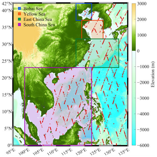
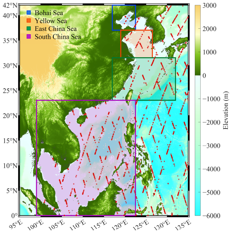
The CSA study area extends from 95°E–135°E and 0–42°N (Figure 1). The CSA regional mean includes all ocean grid cells within this geographical boundary that satisfy the ocean-mask criteria described in Section 3.1. Four major marginal seas within the CSA were defined as individual analysis domains: the Bohai Sea (117.0°E–122.5°E, 37.0°N–42.0°N), Yellow Sea (119.0°E–126.5°E, 31.5°N–37.0°N), East China Sea (117.0°E–132.0°E, 23.0°N–31.5°N), and South China Sea (99.0°E–122.5°E, 0–23.0°N). The CSA encompasses a wide range of marine environments, from the shallow, semi-enclosed Bohai and Yellow Seas to the broad continental shelf of the East China Sea and the shelf–slope–deep-basin system of the South China Sea. The region is also characterized by complex coastlines, numerous islands and straits, and exchanges between the marginal seas and the western North Pacific.

Figure 1. Study area of the China Seas and their Adjacent Oceans (CSA), with the four major marginal-sea analysis domains delineated within the CSA and Jason-1 ground tracks. The background shows land topography and ocean bathymetry, and the red dots indicate Jason-1 along-track observations.

2.2. Data

2.2.1. Along-Track Altimetry Data

The along-track satellite-altimetry data used in this study were obtained from Version 04_00 of the Level-2+ (L2P) Non-Time-Critical (NTC) sea-level anomaly (SLA) products distributed by the Archiving, Validation and Interpretation of Satellite Oceanographic Data (AVISO+; https://www.aviso.altimetry.fr/, accessed on 25 July 2026). The L2P products are generated by applying consistent processing procedures to the 1-Hz single-mission observations from TOPEX/Poseidon (TP), ERS-1/2, Geosat Follow-On (GFO), Envisat, Jason-1 (J1), Jason-2 (J2), Jason-3 (J3), SARAL/AltiKa, CryoSat-2, Sentinel-3A/B, HaiYang-2A/B, and Sentinel-6A (S6A). The processing includes standardized data editing and quality control, together with corrections for dry and wet tropospheric delays, ionospheric delay, sea-state bias, ocean and load tides, solid Earth tide, pole tide, and dynamic atmospheric effects [32,33]. In particular, the Sentinel-6A observations were reprocessed according to the same L2P processing standards applied to the other altimeter missions, ensuring consistency within the multi-mission dataset [33]. Detailed descriptions of the L2P processing and the applied geophysical corrections are provided in the L2P Product Handbook [33].

From the available L2P products, observations from TP, J1, J2, J3, and S6A were selected to construct a continuous satellite-altimetry record covering the period from 1 January 1993 to 23 May 2026. The corresponding data periods, cycle ranges, and overlapping observation intervals between successive missions are summarized in Table 1.

Table 1. Data periods, cycle ranges, and tandem-phase cycle ranges for the satellite altimetry missions used in this study. Tandem-phase cycles indicate the overlapping observation cycles between successive missions used for inter-mission bias estimation. TP-A and TP-B denote the TOPEX/Poseidon Side-A (1992–1999) and Side-B (1999–2002) mission phases, respectively.

Mission	Period (yyyy-mm-dd)	Cycles	Tandem-Phase Cycles
			TP/J1	J1/J2	J2/J3	J3/S6A
TP-A/TP-B	1993-01-01 to 2002-05-04	11–354	344–364
J1	2002-05-04 to 2008-10-29	12–250	1–21	240–259
J2	2008-10-29 to 2016-06-05	12–291		1–20	281–303
J3	2016-06-05 to 2021-12-29	12–216			1–23	207–226
S6A	2021-12-29 to 2026-05-23	42–203				32–51

2.2.2. External Gridded Sea-Level Products

To assess the consistency of the long-term regional sea-level changes derived from the along-track observations, two external gridded satellite-altimetry products were used: the NASA gridded sea-level anomaly (SLA) product distributed by the Physical Oceanography Distributed Active Archive Center (PO.DAAC) and the Copernicus Marine Service (CMEMS) Data Unification and Altimeter Combination System (DUACS) product.

The NASA product provides gridded SLA fields at a spatial resolution of 0.5° × 0.5° and an approximately 7-day temporal resolution, with records available from October 1992 onward. The CMEMS DUACS Level-4 product used in this study provides monthly gridded SLA fields at a spatial resolution of 0.125° × 0.125°, referenced to the 1993–2012 mean sea surface. The CMEMS record used here spans January 1993 to January 2026.

Both products were extracted over the CSA domain, and regional mean SLA series were calculated using the same area-weighting principle applied to the along-track record, accounting for latitude-dependent grid-cell area and ocean fraction. The NASA 7-day SLA fields were averaged to monthly values to match the temporal resolution of the CMEMS and along-track regional records. No additional GIA correction was applied to the NASA or CMEMS records; each product retained its original processing and correction conventions. The resulting regional time series were compared in terms of temporal variability, trend, and acceleration.

2.2.3. Auxiliary Datasets

Auxiliary JMR, AMSR-E, and ERA5 datasets were used to characterize the regional wet tropospheric correction (WTC) uncertainty. Because their temporal coverage differs, the analysis was restricted to the common period from January 2004 to December 2010, during which all three datasets were available. The datasets were processed onto a common monthly 3° × 3° grid and restricted to their common spatial coverage. These auxiliary datasets were not concatenated or extrapolated to construct a continuous WTC record over the full altimetry period.

The gridded GIA correction-rate and 1σ uncertainty fields of Prandi et al. [16] were used to determine the regional GIA correction and uncertainty separately for the CSA and each marginal-sea domain. Both fields were area-weighted over each domain using the same ocean-fraction and latitude-dependent weighting adopted for the regional sea-level records. The resulting GIA correction rates were applied to the corresponding regional sea-level series, and the regional GIA uncertainties were incorporated into the error variance–covariance matrices.

3. Methodology

3.1. Construction of Regional Sea-Level Time Series

The processing workflow consisted of data screening, cycle-scale gridding, regional averaging, inter-mission alignment, and long-term corrections. The same processing procedure was applied to the CSA and the four major marginal-sea analysis domains.

The along-track observations listed in Table 1 were assigned to regular 1° × 1° latitude–longitude grid cells for each satellite cycle. Observations within each cell were averaged to obtain a single grid-cell value, preventing differences in along-track sampling density from introducing additional weighting in the subsequent regional averaging.

The effective ocean fraction of each 1° × 1° grid cell was derived from the high-resolution GEBCO bathymetry. Specifically, $f_{\mathrm{o}\mathrm{c}\mathrm{e}\mathrm{a}\mathrm{n},i}$ is defined as the fraction of GEBCO subcells within grid cell i with water depths greater than 20 m (bathymetric elevations below −20 m). The weight assigned to each grid cell combined its effective ocean fraction with the latitude-dependent grid-cell area and was defined as

$$w_i=f_{\mathrm{o}\mathrm{c}\mathrm{e}\mathrm{a}\mathrm{n},i}\cos {\varphi }_i$$

(1)

where ${\varphi }_i$ is the latitude of the cell center. For a regular latitude–longitude grid with constant angular resolution, the grid-cell area is proportional to $\cos {\varphi }_i$. Thus, the $\cos {\varphi }_i$ term accounts for the decrease in grid-cell area with increasing latitude, while $f_{\mathrm{o}\mathrm{c}\mathrm{e}\mathrm{a}\mathrm{n},i}$ accounts for partial ocean coverage within coastal grid cells.

The regional mean sea level at time $t$ is calculated as

$$\overline{h}\left(t\right)={\displaystyle \frac{\sum _{i\in V\left(t\right)}{h}_i\left(t\right)f_{\mathrm{ocean},i}\cos {\varphi }_i}{\sum _{i\in V\left(t\right)}{f}_{\mathrm{ocean},i}\cos {\varphi }_i}}$$

(2)

where $h_i\left(t\right)$ is the sea-level value of grid cell i at time t, and V(t) denotes the set of grid cells containing observations at that time. The weights were normalized over the grid cells included at each time step. Therefore, partially ocean-covered coastal cells received proportionally smaller weights than cells with greater ocean coverage at the same latitude. For example, at the same latitude, a grid cell with an effective ocean fraction of 0.20 receives only 21% of the weight assigned to a cell with an effective ocean fraction of 0.95.

Only grid cells containing valid observations at a given time step are included in the regional mean, and the weights are renormalized over the available cells. Unsampled cells are not spatially interpolated, and missing regional time steps are retained as missing values without temporal interpolation.

The regional SLA time series from successive missions were aligned using observations acquired during the TP/J1, J1/J2, J2/J3, and J3/S6A tandem phases. The estimation of the inter-mission offsets and their uncertainties is described in Section 3.2.

Following inter-mission alignment, the regional time series were corrected for the early-TOPEX drift and GIA. The early-TOPEX correction accounted for both the TP-A drift and the datum difference between TP-A and TP-B following the recommended processing strategy for the TOPEX/Poseidon mission. Regional GIA correction rates were obtained by area-weighting the gridded GIA correction-rate field over each study region. The uncertainties associated with inter-mission offsets, early-TOPEX effects, GIA, orbit determination, WTC, and terrestrial reference-frame stability were incorporated into the error variance–covariance matrices described in Section 3.2 and propagated to the trend and acceleration estimates.

The resulting regional SLA time series span January 1993 to May 2026 for the CSA and the four marginal-sea analysis domains. These regional time series formed the basis for estimating long-term trends, accelerations, and annual and semiannual variability and for comparison with the NASA and CMEMS gridded products.

3.2. Estimation of Trends, Accelerations, and Associated Uncertainties

Long-term changes in the regional sea-level time series were estimated using a regression model consisting of a linear trend, a quadratic term, and annual and semiannual harmonic components. The model was formulated as:

$$\eta \left(t\right)=a+bt+{\displaystyle \frac{1}{2}}c{t}^2+A_1\cdot \mathrm{s}\mathrm{i}\mathrm{n}\left(2\pi t\right)+B_1\cdot \mathrm{c}\mathrm{o}\mathrm{s}\left(2\pi t\right)+A_2\cdot \mathrm{s}\mathrm{i}\mathrm{n}\left(4\pi t\right)+B_2\cdot \mathrm{c}\mathrm{o}\mathrm{s}\left(4\pi t\right)+\epsilon \left(t\right)$$

(3)

where $\eta \left(t\right)$ is the regional sea-level time series; $t$ is time in years from January 1993; $a$ is the intercept; $b$ is the linear trend; $c$ is the acceleration; $A_1$ and $B_1$ are the annual harmonic coefficients; $A_2$ and $B_2$ are the semiannual harmonic coefficients; and $\epsilon \left(t\right)$ is the residual.

The regionalized uncertainty budget was constructed by characterizing the magnitudes, active periods, and temporal correlation structures of the major satellite-altimetry measurement and processing errors affecting the regional sea-level time series. Following the measurement-error uncertainty-budget framework of Ablain et al. [19], the contributing errors were represented as time-correlated, bias, or drift errors. Time-correlated errors included residual altimeter and geophysical-correction errors, WTC uncertainty, and orbit-determination uncertainty. Bias errors represented uncertainties associated with inter-mission alignment and the TP-A/TP-B transition, whereas drift errors included uncertainties in the early-TOPEX correction, the terrestrial reference frame, and the GIA correction. For each error source, an individual covariance matrix was constructed according to its uncertainty amplitude, active period, and prescribed temporal correlation structure. Following Ablain et al. [19] and Guérou et al. [6], cross-covariances between separately modeled error sources were not included, and the total measurement-error covariance matrix was obtained as:

$${\mathrm{C}}_{\eta }={\displaystyle \sum _{k=1}^K}{\mathrm{C}}_{\eta }^{\left(k\right)}$$

(4)

where ${\mathrm{C}}_{\eta }^{\left(k\right)}$ denotes the covariance contribution of the $k$-th error source, and $K$ is the total number of error sources included in the regional uncertainty budget. This treatment represents a simplifying assumption of the uncertainty model rather than evidence that the underlying error processes are strictly statistically independent, because reliable quantitative estimates of cross-covariances among these heterogeneous error sources are not presently available.

For each continuously acting time-correlated error source, an individual covariance matrix was constructed from its uncertainty amplitude, active period, and prescribed temporal correlation structure. Following Ablain et al. [19] and Guérou et al. [6], the covariance between errors at times $t_i$ and $t_j$ was represented using a Gaussian correlation function:

$$C_{ij}={\sigma }_i{\sigma }_j\exp \left[-{\displaystyle \frac{1}{2}}{\left({\displaystyle \frac{\left|t_i-t_j\right|}{\lambda }}\right)}^2\right]$$

(5)

where $C_{ij}$ is the covariance between errors at epochs $t_i$ and $t_j$; ${\sigma }_i$ and ${\sigma }_j$ are the corresponding one-standard-deviation uncertainty amplitudes; and $\lambda$ is the temporal correlation scale.

For each time-correlated uncertainty component, the covariance model requires an uncertainty amplitude and a temporal correlation scale. The uncertainty amplitude describes the magnitude of the error, whereas the correlation scale describes its temporal persistence. These two quantities were determined separately in this study. The correlation scales were adopted according to the error classes established in previous satellite-altimetry uncertainty assessments [6,19], whereas the uncertainty amplitudes were estimated from the regional data where suitable observations were available or adopted from previous assessments for mission-wide error sources.

Following Ablain et al. [19], residual time-correlated errors were separated into two classes according to their characteristic timescales: errors with variability shorter than approximately 2 months and errors with variability between approximately 2 months and 1 year. These classes mainly represent residual errors associated with altimeter measurements and geophysical corrections that remain after standard processing. Guérou et al. [6] retained the same error classes in the updated satellite-altimetry uncertainty budget. In the covariance model used here, correlation scales of 2 months and 1 year were assigned to the short- and medium-timescale residual-error components, respectively.

The 1-year correlated-error component is distinct from the deterministic annual harmonic included in Equation (3). The annual and semiannual components are removed when the regression residuals are formed. The 1-year correlated component represents residual measurement and correction variability at timescales between approximately 2 months and 1 year that remains after removal of the fitted seasonal components.

The uncertainty amplitudes of these two residual-error components were estimated from the regional sea-level residuals. For each analysis domain, the fitted trend, acceleration, annual component, and semiannual component were first removed from the regional sea-level series. A Lanczos filter was then applied to separate residual variability at timescales shorter than 2 months from variability between 2 months and 1 year. The standard deviation of each filtered component was calculated separately for each mission period and adopted as the one-standard-deviation uncertainty amplitude of the corresponding residual-error component.

Because the residual series may also contain unresolved oceanographic variability, these empirically estimated amplitudes are treated as conservative proxies for the regional measurement and processing uncertainties.

WTC stability was treated as a separate long-timescale correlated uncertainty. Previous comparisons among microwave-radiometer and atmospheric-reanalysis wet tropospheric corrections have shown slowly varying differences over periods of approximately 5–10 years. Ablain et al. [19] therefore represented WTC stability uncertainty using a 5-year Gaussian correlation scale, which was subsequently retained in the updated uncertainty framework of Guérou et al. [6]. The same 5-year correlation scale was adopted here.

The WTC uncertainty amplitude was estimated separately for each analysis domain using the regional JMR-, AMSR-E-, and ERA5-derived series. Because the three datasets have different temporal coverage, the calculation was restricted to their common January 2004–December 2010 period and common spatial support. Pairwise differences among the three regional WTC series were used to characterize their relative stability and were combined to obtain the regional one-standard-deviation WTC uncertainty amplitude in equivalent sea-level height. For the Bohai Sea, where the common spatial support of all three datasets was insufficient, the uncertainty amplitude was estimated using the combined Bohai–Yellow Sea common support.

The common 2004–2010 period was used only to estimate the regional WTC uncertainty amplitude. It was not used to determine the 5-year correlation scale. The estimated regional amplitude was propagated over the complete altimetry record using the prescribed 5-year Gaussian covariance model in Equation (5). Sensitivity to this prescribed timescale was evaluated by repeating the CSA calculation with WTC correlation scales of 3, 5, 7, and 10 years while keeping the uncertainty amplitude and all other covariance inputs unchanged.

Orbit-determination uncertainty was represented as a long-timescale correlated error. Comparisons among independent precise orbit solutions have shown differences on approximately 10-year timescales, including errors associated with the modeling of the time-varying gravity field [19,20,21,22]. Following these assessments and Guérou et al. [6], a 10-year Gaussian correlation scale was adopted for the orbit-determination uncertainty. One-standard-deviation amplitudes of 1.1 mm for the TP period and 0.5 mm for the Jason and Sentinel periods were adopted from the established altimetry uncertainty framework rather than estimated from the regional CSA residuals.

Each observation epoch was assigned the orbit uncertainty amplitude corresponding to its mission period, and the temporal covariance between epochs was calculated using Equation (5) with the 10-year correlation scale.

Inter-mission offsets and their uncertainties were estimated from the TP/J1, J1/J2, J2/J3, and J3/S6A tandem phases. For each transition, regional sea-level observations from the two missions were paired over their common tandem period. A tandem-phase difference series was constructed using a consistent mission order.

$$d_i={\eta }_{\mathrm{e}\mathrm{a}\mathrm{r}\mathrm{l}\mathrm{y},i}-{\eta }_{\mathrm{l}\mathrm{a}\mathrm{t}\mathrm{e},i}$$

(6)

where $d_i$ denotes the tandem-phase difference at the $i$-th paired observation.

All valid paired observations within each tandem phase were retained. The inter-mission offset was estimated as the arithmetic mean of the tandem-phase difference series.

$$\widehat{\Delta }={\displaystyle \frac{1}{N}}\stackrel{N}{\underset{i=1}{\sum d_i}}$$

(7)

where $\widehat{\Delta }$ is the estimated inter-mission offset, and $N$ is the number of valid tandem differences.

The estimated offset was used for datum alignment between the two successive mission segments. The dispersion of the individual tandem differences was quantified using the sample standard deviation.

$$s_{\Delta }=\sqrt{{\displaystyle \frac{1}{N-1}}\stackrel{N}{\underset{i=1}{\sum {\left(d_i-\widehat{\Delta }\right)}^2}}}$$

(8)

The sample standard deviation describes the variability of the individual tandem differences rather than the uncertainty of their estimated mean. Because successive tandem observations may be temporally correlated, the number of statistically independent observations can be smaller than the total number of paired observations. Following the AR(1)-based treatment used by Guérou et al. [6], an effective sample size was therefore estimated from the lag-1 autocorrelation of each tandem-phase difference series.

$$n_{\mathrm{e}\mathrm{f}\mathrm{f}}=\mathrm{m}\mathrm{i}\mathrm{n}\left[N,\mathrm{m}\mathrm{a}\mathrm{x}\left(2,N{\displaystyle \frac{1-{\rho }_1}{1+{\rho }_1}}\right)\right]$$

(9)

where $n_{\mathrm{e}\mathrm{f}\mathrm{f}}$ is the effective sample size, and ${\rho }_1$ is the lag-1 autocorrelation of the tandem-phase difference series.

The effective sample size was constrained not to exceed the actual number of paired observations and not to fall below two. Unrounded values were retained in the calculations, whereas rounded values are reported in Table 2.

Table 2. Estimated inter-mission offset uncertainties for adjacent satellite-altimetry mission pairs during the tandem phases in the CSA.

Tandem Phase	TP/J1	J1/J2	J2/J3	J3/S6A
Number of tandem differences, N	21	19	23	19
Effective sample size, neff	6	19	23	9
Offset uncertainty (1σ, mm)	1.970	0.910	0.422	1.000
Student-t U90 (mm)	4.002	1.578	0.724	1.854

Note: Effective sample sizes are rounded to the nearest integer for presentation; the unrounded values were retained in the uncertainty calculations.

The standard uncertainty of the estimated mean offset was then calculated using the sample dispersion and the effective number of independent observations.

$$u_{\Delta }={\displaystyle \frac{s_{\Delta }}{\sqrt{n_{\mathrm{e}\mathrm{f}\mathrm{f}}}}}$$

(10)

This quantity represents the uncertainty of the estimated mean transition offset. Because the effective number of independent observations is limited for the tandem phases, the corresponding two-sided 90% uncertainty was calculated using the Student-t distribution.

$$U_{90}=t_{0.95,n_{\mathrm{e}\mathrm{f}\mathrm{f}}-1}{u}_{\Delta }$$

(11)

where the Student-t coefficient is evaluated using the effective degrees of freedom. The standard uncertainty in Equation (10) was used in the covariance propagation, whereas Equation (11) was used only to report the 90% uncertainty of each transition-offset estimate. The resulting effective sample sizes and transition uncertainties are summarized in Table 2.

The uncertainty of an inter-mission offset was treated differently from independent cycle-level noise. Any error remaining in the estimated datum transition affects all subsequent observations linked through that transition in the same way. Each transition uncertainty was therefore represented as a coherent mission-dependent bias in the covariance model.

For each transition, an indicator vector was defined with zero values before the transition and unit values from the transition onward. The covariance contribution of an individual transition was defined as

$$C_{\Delta ,k}=u_{\Delta ,k}^2{h}_k{h}_k^T$$

(12)

where $C_{\Delta ,k}$ is the covariance contribution of transition $k$, $u_{\Delta ,k}$ is its standard uncertainty, and $h_k$ is the corresponding indicator vector.

This formulation represents the transition uncertainty as fully coherent over the affected part of the time series and assigns no contribution to observations preceding the transition.

Because the continuous regional record was constructed by sequentially linking TP, J1, J2, J3, and S6A, the covariance contributions from the four mission transitions were combined as

$$C_{\mathrm{o}\mathrm{f}\mathrm{f}\mathrm{s}\mathrm{e}\mathrm{t}}=\stackrel{4}{\underset{k=1}{\sum C_{\Delta ,k}}}$$

(13)

Thus, later mission segments include the uncertainty contributions associated with the preceding datum transitions. This preserves the sequential structure of the multi-mission record when the transition uncertainties are propagated to the estimated trend and acceleration.

Early-TOPEX uncertainty was represented by the TP-A/TP-B offset uncertainty together with the residual drift uncertainties during the TP-A and TP-B periods. The TP-A/TP-B offset uncertainty was prescribed as 2.0 mm (1σ). Residual drift uncertainties of 0.7 and 0.1 mm yr⁻¹ were prescribed for the TP-A and TP-B periods, respectively [6,19,26]. The corresponding covariance matrices were represented as linear drift terms over their respective active periods.

The ITRF realization uncertainty was represented as a linear drift over the complete record. A one-standard-deviation drift uncertainty of 0.1 mm yr⁻¹ was adopted following established altimetry uncertainty frameworks and previous assessments of orbit and reference-frame stability [6,19,20,21].

Regional GIA correction rates and their associated 1σ drift-rate uncertainties were obtained separately for the CSA and each of the four marginal-sea analysis domains by area-weighting the corresponding global gridded GIA fields [16,28]. The area-weighted regional GIA correction was applied to the corresponding regional sea-level time series, while the region-specific 1σ GIA uncertainty was represented as a linear drift and propagated through the covariance model over the complete record. The regional GIA correction rates and the associated uncertainty values are reported for each analysis domain in Section 4.3.

The same covariance formulation was applied to the CSA and the four marginal-sea domains using region-specific WTC, inter-mission transition, and GIA parameters together with the common mission-wide orbit, ITRF, and early-TOPEX uncertainty representations.

After the covariance matrices for the individual uncertainty sources had been constructed, Equation (4) was used to obtain the total measurement-error covariance matrix of the regional sea-level time series. The diagonal elements represent the variances of individual sea-level estimates, whereas the off-diagonal elements describe the temporal covariance between observations. The covariance matrix was then propagated through the least-squares estimator to obtain the covariance matrix of the estimated regression parameters,

$${\mathrm{C}}_{\widehat{\beta }}={\left({\mathrm{X}}^T\mathrm{X}\right)}^{-1}{\mathrm{X}}^T{\mathrm{C}}_{\eta }\mathrm{X}{\left({\mathrm{X}}^T\mathrm{X}\right)}^{-1}$$

(14)

where $\mathrm{X}$ is the regression design matrix, and ${\mathrm{C}}_{\widehat{\beta }}$ is the covariance matrix of the estimated regression parameters. The diagonal elements of ${\mathrm{C}}_{\widehat{\beta }}$ represent the variances of the estimated regression parameters, and the corresponding one-standard-deviation uncertainties of the trend and acceleration were obtained from their square roots. Assuming Gaussian errors, these standard uncertainties were multiplied by 1.645 and are reported as covariance-propagated 90% uncertainties. These values quantify the uncertainty in the fitted trend and acceleration induced by the modeled satellite-altimetry measurement and processing error covariance. To quantify how each uncertainty source contributes to the covariance-propagated uncertainties of the estimated trend and acceleration, the covariance matrix of each source was propagated separately through Equation (14). For comparison, residual-based 90% confidence intervals were estimated independently from the regression residuals. These intervals characterize the statistical precision of the estimated parameters under the unresolved residual variability and do not explicitly propagate the identified measurement and processing error sources. The covariance-propagated uncertainties and residual-based confidence intervals therefore represent different aspects of parameter uncertainty and are reported separately rather than combined.

4. Results

4.1. Inter-Mission Tandem-Phase Offsets and Their Uncertainties

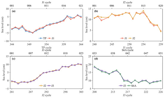
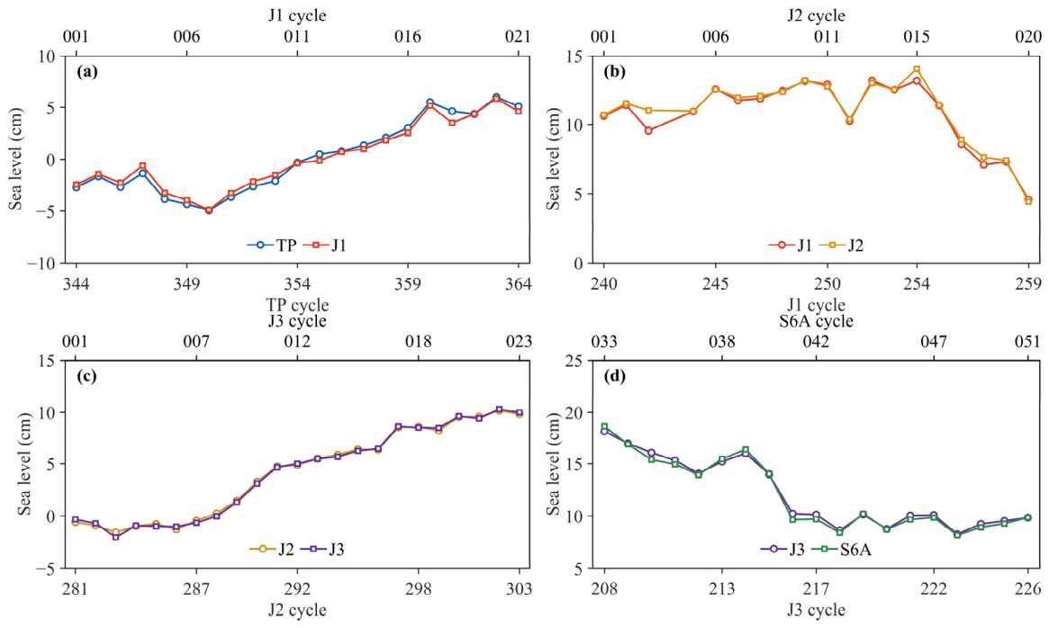
Figure 2 shows the regional sea-level observations from adjacent missions during the TP/J1, J1/J2, J2/J3, and J3/S6A tandem phases, with the corresponding observation periods and tandem cycles summarized in Table 1. Within each tandem phase, the paired missions show closely consistent cycle-to-cycle sea-level variations, while systematic differences in their relative levels are evident for some mission transitions. These tandem observations provide the basis for estimating the inter-mission offsets from the mean differences between the paired missions and for aligning the successive mission records.

Figure 2. Regional sea-level observations from adjacent satellite-altimetry missions during their tandem phases: (a) TP/J1, (b) J1/J2, (c) J2/J3, and (d) J3/S6A.

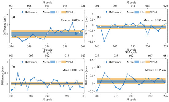
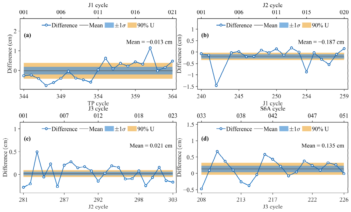
Figure 3 further presents the tandem-phase difference series used to estimate the inter-mission offsets and their uncertainties for the four mission transitions. The mean offsets are −0.013 cm for TP/J1, −0.187 cm for J1/J2, 0.021 cm for J2/J3, and 0.135 cm for J3/S6A. The difference series show different levels of cycle-to-cycle variability among the four transitions, which is reflected in the corresponding uncertainty ranges of the estimated offsets. The magnitude of the mean offset is not directly related to its uncertainty; for example, a mean difference close to zero can still be associated with appreciable variability during the tandem phase. This distinction is important because the estimated offsets are used for inter-mission alignment, whereas their uncertainties are propagated separately in the error variance–covariance matrix.

Figure 3. Difference series and estimated inter-mission offsets during the tandem phases of adjacent satellite-altimetry missions. The mean offset is annotated in each panel, and the shaded bands denote the corresponding 1σ and 90% uncertainty of the estimated offset. (a) TP/J1, (b) J1/J2, (c) J2/J3, and (d) J3/S6A.

Table 2 summarizes the uncertainties of the four inter-mission offsets. TP/J1 has the largest uncertainty, with a 1σ value of 1.970 mm and a Student-t U₉₀ of 4.002 mm. Its effective sample size is substantially smaller than the 21 available tandem differences because of the temporal dependence within the difference series. J3/S6A also shows a reduced effective sample size and has a 1σ uncertainty of 1.000 mm and a U₉₀ of 1.854 mm. The J1/J2 and J2/J3 transitions have smaller 1σ uncertainties of 0.910 and 0.422 mm, respectively, with J2/J3 remaining the best-constrained transition.

4.2. Comparison with External Gridded Sea-Level Products

The regional sea-level time series derived from the along-track observations was compared with the corresponding regional time series derived from the NASA and CMEMS gridded SLA products to assess the consistency of long-term regional sea-level change across different satellite-altimetry processing frameworks.

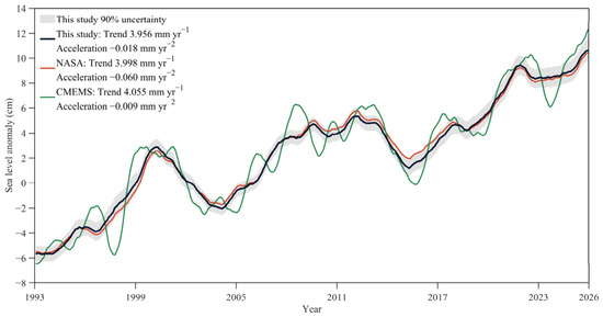
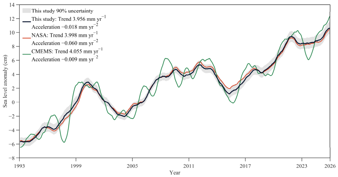
As shown in Figure 4, the three CSA records exhibit a sustained long-term rise and broadly similar low-frequency variability over the common comparison period. The along-track and NASA series remain close through much of the record, whereas the CMEMS series shows larger-amplitude departures during the late 1990s, 2008–2010, 2015–2017, and after 2022. These differences are more evident in the amplitude of regional variability than in the estimated long-term trends.

Figure 4. Comparison of the regional sea-level time series derived from the along-track observations with those derived from the NASA and CMEMS gridded sea-level anomaly products over their common period from January 1993 to January 2026.

For the common January 1993–January 2026 period, the trend estimated from the along-track record is 3.956 mm yr⁻¹, compared with 3.998 mm yr⁻¹ for NASA and 4.055 mm yr⁻¹ for CMEMS. The corresponding acceleration estimates are −0.018, −0.006, and −0.009 mm yr⁻², respectively. Thus, the three products give closely comparable long-term rates and consistently small acceleration estimates despite differences in their short- and interannual-scale variability. The values for the along-track record differ slightly from the full-record estimates reported in Section 4.4 because Figure 4 is restricted to the common comparison period ending in January 2026.

4.3. Regionalized Uncertainty Budget

The measurement and processing uncertainties associated with the resulting CSA record were subsequently quantified. Table 3 summarizes the error sources and uncertainty parameters used to construct its error variance–covariance matrix. Following their temporal characteristics, the uncertainty sources are represented as temporally correlated errors, mission-transition biases, or long-term drifts. The correlated errors cover different timescales: high-frequency altimeter and geophysical-correction residuals are characterized by a 2-month correlation scale, annual-scale geophysical-correction residuals by a 1-year scale, WTC uncertainty by a 5-year scale, and orbit-determination uncertainty by a 10-year scale. Their amplitudes also differ among error sources and mission periods. The high-frequency residual uncertainty decreases from 1.7 mm during the TP period to 1.0 mm during the J3/S6A period, while the annual-scale residual uncertainty ranges from 1.1 to 1.4 mm. The WTC uncertainty is 1.1 mm, whereas the orbit-determination uncertainty decreases from 1.1 mm during the TP period to 0.5 mm for the subsequent missions.

Table 3. Measurement and processing error sources and uncertainty parameters used to construct the error variance–covariance matrix for the CSA regional sea-level record.

Source of Uncertainty	Type of Error	Uncertainty Used in This Study	Method/References
High-frequency altimeter and geophysical correction residuals	Correlated errors λ = 2 months	uσ = 1.7 mm over the TP period; uσ = 1.2 mm over the J1 period; uσ = 1.1 mm over the J2 period; uσ = 1.0 mm over the J3/S6A period	This study; Guérou et al. [6]; Ablain et al. [19]
Annual-scale geophysical correction residuals	Correlated errors λ = 1 year	uσ = 1.4 mm over the TP period; uσ = 1.2 mm over the J1 period; uσ = 1.1 mm over the J2 period; uσ = 1.1 mm over the J3/S6A period	This study; Guérou et al. [6]; Ablain et al. [19]
Wet tropospheric correction stability uncertainty	Correlated errors λ = 5 years	uσ = 1.1 mm over the entire period	This study; Guérou et al. [6]; Ablain et al. [19]
Orbit determination uncertainty	Correlated errors λ = 10 years	uσ = 1.1 mm over the TP period; uσ = 0.5 mm over the Jason/Sentinel period	Couhert et al. [20]; Rudenko et al. [21,22]
Mission-transition calibration offset uncertainty	Bias	u∆ = 2.0 mm for TP-A/TP-B; u∆ = 2.0 mm for TP/J1; u∆ = 0.9 mm for J1/J2; u∆ = 0.4 mm for J2/J3; u∆ = 1.0 mm for J3/S6A	This study; Table 2
ITRF uncertainty	Drift	uσ = 0.1 mm yr−1 over 1993–present	Couhert et al. [20]
GIA correction uncertainty	Drift	uσ = 0.1 mm yr−1 for the CSA region	This study; Prandi et al. [16]; Spada [28]
TOPEX early-mission correction uncertainty	Drift	uσ = 0.7 mm yr−1 over the TP-A period; uσ = 0.1 mm yr−1 over the TP-B period	Ablain et al. [19]; Beckley et al. [26]

Note: Uncertainty amplitudes are rounded to one decimal place for presentation, while unrounded values were retained in covariance calculations.

The remaining uncertainty components represent discontinuities or long-term effects in the regional record. Inter-mission offset uncertainties are treated as transition-specific bias terms, with amplitudes determined separately for the successive mission transitions. ITRF and CSA GIA uncertainties are represented as drift terms with rounded 1σ amplitudes of 0.1 mm yr⁻¹. The residual early-TOPEX drift uncertainty is 0.7 mm yr⁻¹ during TP-A and 0.1 mm yr⁻¹ during TP-B. Thus, the uncertainty budget contains error components that differ not only in magnitude but also in their temporal characteristics and representation. These source-specific parameters determine the individual covariance components that are combined to form the CSA error variance–covariance matrix. The uncertainty amplitudes reported in Table 3 are rounded to one decimal place for presentation, while the unrounded values were retained in the covariance calculations.

The spatially dependent uncertainty components were evaluated separately for each analysis domain. Table 4 summarizes the region-specific WTC, inter-mission transition, and GIA uncertainty estimates, together with the signed GIA correction rates for the CSA and the four marginal-sea domains. The remaining mission-wide and reference-frame uncertainty components retain the common representations summarized in Table 3.

Table 4. Region-dependent uncertainty estimates and signed GIA correction rates used in the covariance calculations for the CSA and four marginal-sea domains.

Region	WTC uσ (mm)	TP/J1 u∆ (mm)	J1/J2 u∆ (mm)	J2/J3 u∆ (mm)	J3/S6A u∆ (mm)	GIA uσ (mm yr−1)	Signed GIA Correction Rate (mm yr−1)
CSA	1.134	1.970	0.910	0.422	1.000	0.108	−0.155
Bohai Sea	1.172	4.502	2.590	1.476	2.584	0.145	−0.599
Yellow Sea	0.866	2.399	1.258	1.699	1.724	0.141	−0.525
East China Sea	0.286	1.788	0.760	1.334	0.794	0.131	−0.391
South China Sea	1.609	2.852	1.139	0.658	0.922	0.085	−0.093

Note: WTC, inter-mission transition, and GIA uncertainty values are one-standard-deviation (1σ) estimates. The signed GIA correction rates are the area-weighted regional corrections applied to the corresponding sea-level time series.

The region-specific uncertainty estimates show clear differences among the five records. WTC uncertainty ranges from 0.286 mm in the East China Sea to 1.609 mm in the South China Sea, while GIA uncertainty ranges from 0.085 mm yr⁻¹ in the South China Sea to 0.145 mm yr⁻¹ in the Bohai Sea. The signed GIA correction rates also vary among the analysis domains, from −0.093 mm yr⁻¹ in the South China Sea to −0.599 mm yr⁻¹ in the Bohai Sea, with a CSA value of −0.155 mm yr⁻¹. The inter-mission transition uncertainties likewise vary by region and mission pair, with the Bohai Sea generally showing the largest values for several transitions. These differences demonstrate that the spatially dependent uncertainty parameters are estimated separately for each region rather than inherited from a single CSA-wide set of amplitudes. The rounded CSA GIA uncertainty reported in Table 3 is therefore not imposed on the marginal-sea records; the region-specific values in Table 4 are used in the corresponding covariance calculations.

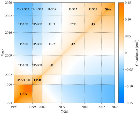
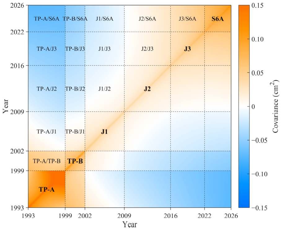
The uncertainty components and parameters summarized in Table 3 were used to construct the error variance–covariance matrix for the CSA regional sea-level record over January 1993–May 2026 (Figure 5). The largest covariance values occur along the main diagonal and its vicinity, primarily reflecting the short- and medium-timescale correlated errors. Broader off-diagonal structures result from errors with longer correlation timescales and from drift uncertainties. Relatively large covariance structures are present during the early TOPEX period, consistent with the larger early-TOPEX correction uncertainty and the TP-A/TP-B transition uncertainty. Changes in the covariance structure are also evident across the subsequent mission periods, reflecting differences in the temporal characteristics of the modeled error components and the uncertainties associated with successive mission transitions. The resulting matrix retains these temporal error correlations throughout the CSA record, which are subsequently propagated into the uncertainties of the estimated CSA sea-level trend and acceleration.

Figure 5. Error variance–covariance matrix of the measurement and processing errors in the CSA regional sea-level time series over the altimetry period from January 1993 to May 2026. The labeled segments indicate the successive TP-A, TP-B, J1, J2, J3, and S6A mission periods, and the dashed lines indicate their temporal boundaries.

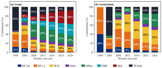
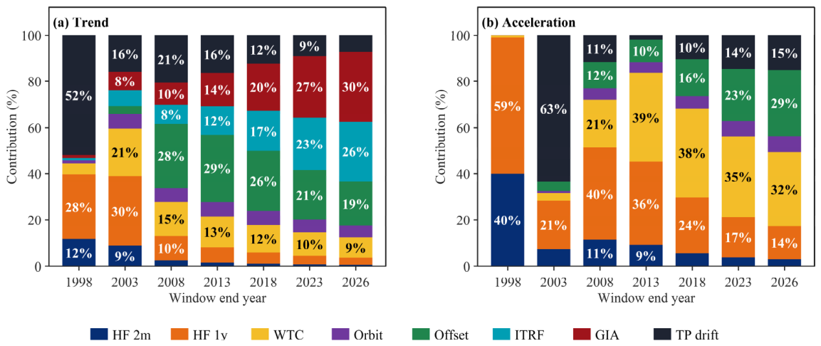
The error variance–covariance components described above were propagated to the trend and acceleration estimates to quantify the contribution of each uncertainty source. Figure 6 shows the relative contributions to the trend and acceleration variances as the record is extended from January 1993 to different end years.

Figure 6. Relative contributions of individual uncertainty sources to the CSA trend and acceleration variances for records ending in different years: (a) trend; (b) acceleration.

For the trend variance (Figure 6a), TP drift and annual-scale residual errors dominate the record ending in 1998, contributing approximately 52% and 28%, respectively. Their relative contributions decrease as the record length increases, whereas the contributions from the longer-timescale uncertainty components become more prominent. For the complete record ending in 2026, GIA and ITRF are the two largest contributors, accounting for approximately 30% and 26% of the trend variance, respectively, followed by inter-mission offset uncertainty at approximately 19%. WTC and TP drift each contribute approximately 9%. This shift reflects the different temporal structures of the uncertainty components: errors confined to the early TOPEX period become less influential as the record is extended, whereas long-term drift uncertainties, particularly GIA and ITRF, have a greater influence on the trend estimated over the full record.

The acceleration variance shows a different dependence on record length (Figure 6b). Annual-scale residual errors and TP drift dominate the shorter records, whereas WTC and inter-mission offset uncertainties become major contributors as the record is extended. Under the adopted 5-year WTC correlation scale, WTC contributes approximately 38%, 35%, and 32% of the acceleration variance for records ending in 2018, 2023, and 2026, respectively. For the complete record, inter-mission offset uncertainty contributes approximately 29%, followed by TP drift (15%) and annual-scale residual errors (14%). The difference from the trend variance reflects the sensitivity of acceleration estimates to the temporal covariance structure of the errors, particularly long-timescale correlated errors and offsets between successive missions. The sensitivity test yields covariance-propagated 90% acceleration uncertainties of 0.031–0.033 mm yr⁻² when the WTC correlation scale is varied from 3 to 10 years. The largest contribution shifts from inter-mission offset uncertainty at correlation scales of 3 and 10 years to WTC at 5 and 7 years.

4.4. Regional Sea-Level Trends and Accelerations in the CSA and Its Major Marginal Seas

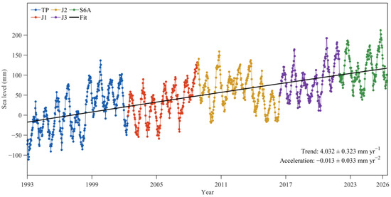
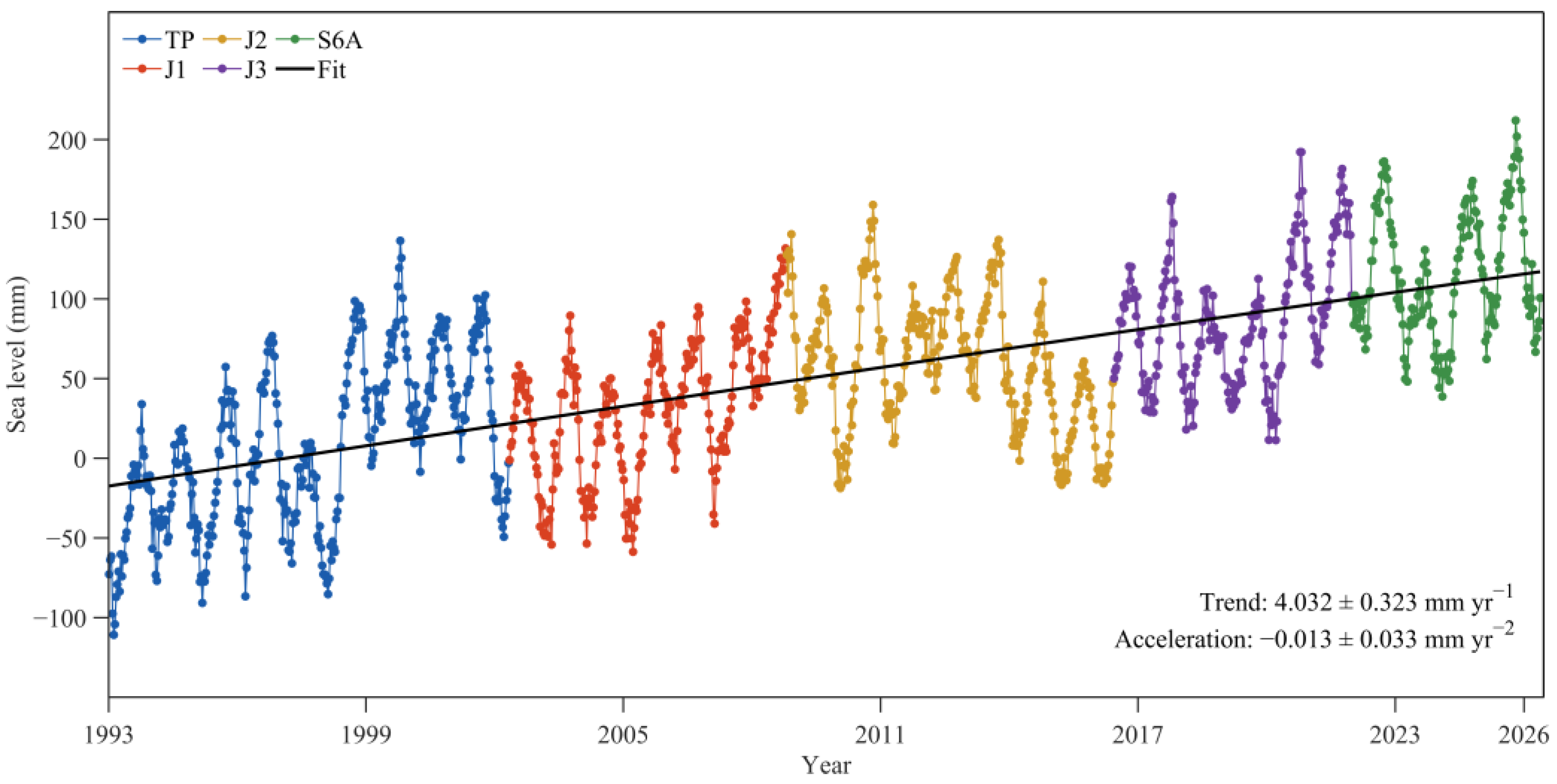
Figure 7 shows the continuous CSA regional sea-level record constructed from the successive TP, J1, J2, J3, and S6A observations. Pronounced short-term and interannual variability is superimposed on a persistent long-term rise, and the successive mission segments follow a consistent trajectory after inter-mission alignment.

Figure 7. CSA regional sea-level time series and fitted long-term sea-level change for January 1993–May 2026. The estimated trend and acceleration and their covariance-propagated 90% uncertainties are annotated in the panel.

For January 1993–May 2026, the estimated CSA sea-level trend is 4.032 ± 0.323 mm yr⁻¹, corresponding to a covariance-propagated 90% uncertainty range of 3.709–4.355 mm yr⁻¹. The acceleration is −0.013 ± 0.033 mm yr⁻², with a corresponding range of −0.046–0.020 mm yr⁻². The trend remains positive over its 90% uncertainty range, whereas the acceleration is not distinguishable from zero within the corresponding uncertainty. Relative to the common-period analysis used for the external-product comparison in Figure 4, extending the along-track record through May 2026 changes the estimated trend from 3.956 to 4.032 mm yr⁻¹ and the acceleration from −0.018 to −0.013 mm yr⁻². These results indicate a robust long-term rise in CSA regional sea level over the satellite-altimetry period, while the estimated acceleration remains small relative to its propagated uncertainty.

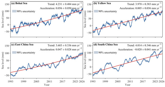
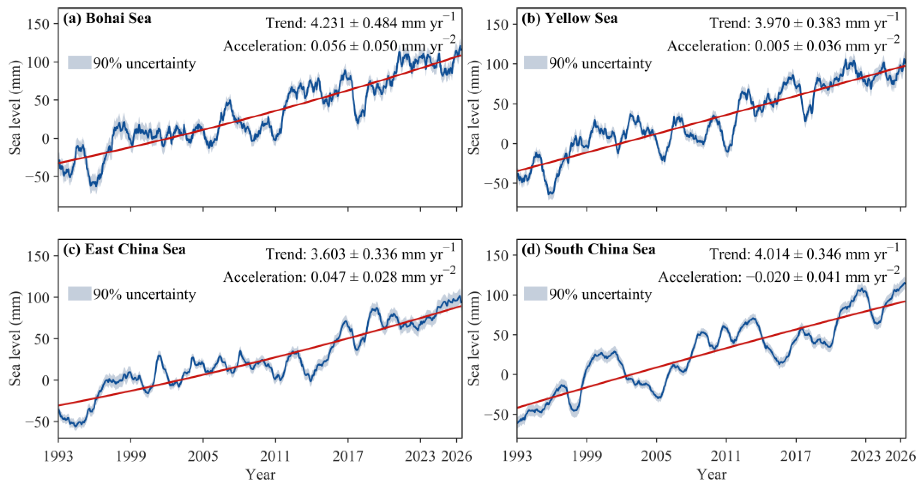
The four marginal-sea records reveal substantial regional differences within the broader CSA domain (Figure 8). All four seas exhibit positive long-term trends, ranging from 3.603 ± 0.336 mm yr⁻¹ in the East China Sea to 4.231 ± 0.484 mm yr⁻¹ in the Bohai Sea. The Yellow and South China Sea trends are 3.970 ± 0.383 and 4.014 ± 0.346 mm yr⁻¹, respectively. Despite these regional differences in magnitude, the covariance-propagated 90% uncertainty ranges remain above zero for all four seas, indicating consistently positive long-term sea-level trends across the marginal-sea records.

Figure 8. Regional sea-level time series and fitted long-term sea-level changes for the four major marginal seas from January 1993 to May 2026. The blue lines show the regional sea-level time series, the red lines show the fitted long-term changes, and the gray shading denotes the covariance-propagated 90% uncertainty. (a) Bohai Sea, (b) Yellow Sea, (c) East China Sea, and (d) South China Sea.

The acceleration estimates exhibit greater regional differences. The Bohai and East China Seas have positive accelerations of 0.056 ± 0.050 and 0.047 ± 0.028 mm yr⁻², respectively, whereas the Yellow Sea estimate is close to zero at 0.005 ± 0.036 mm yr⁻² and the South China Sea has a small negative estimate of −0.020 ± 0.041 mm yr⁻². The covariance-propagated 90% uncertainty ranges include zero for the Yellow and South China Seas, whereas those for the Bohai and East China Seas remain above zero, although the lower bound for the Bohai Sea is close to zero. Consistent with these estimates, positive curvature is more apparent in the Bohai and East China Sea records, while the Yellow and South China Sea records show little curvature over the study period. All four records also exhibit substantial short-term and interannual variability superimposed on their long-term rise.

4.5. Regional Sea-Level Change, Uncertainty, and Seasonal Variability

Table 5 compares the covariance-propagated 90% uncertainties with the residual-based 90% confidence intervals for the regional trend and acceleration estimates. For the trend, the covariance-propagated uncertainties are consistently larger than the residual-based intervals in all five regions, with pronounced differences for the CSA (±0.323 versus ±0.146 mm yr⁻¹), East China Sea (±0.336 versus ±0.149 mm yr⁻¹), and South China Sea (±0.346 versus ±0.142 mm yr⁻¹); nevertheless, all covariance-propagated trend intervals remain above zero. For acceleration, the relationship is less uniform: the covariance-propagated uncertainties are smaller than the residual-based intervals in four of the five regions, while the statistical significance differs between the two estimates only for the Bohai Sea, where the covariance-propagated interval remains slightly above zero but the residual-based interval includes zero. The East China Sea acceleration remains positive under both uncertainty estimates, whereas the intervals for the CSA, Yellow Sea, and South China Sea include zero.

Table 5. Comparison of regional trend and acceleration estimates with covariance-propagated 90% uncertainties and residual-based 90% confidence intervals for the CSA and its four marginal seas. “cov” denotes the parameter uncertainty obtained by propagating the modeled measurement and processing error covariance matrix, whereas “res” denotes the confidence interval estimated independently from the regression residuals.

Region	Trend Cov (mm yr−1)	Trend Res (mm yr−1)	Acceleration Cov (mm yr−2)	Acceleration Res (mm yr−2)
CSA	4.032 ± 0.323	4.032 ± 0.146	−0.013 ± 0.033	−0.013 ± 0.034
Bohai Sea	4.231 ± 0.484	4.231 ± 0.340	0.056 ± 0.050	0.056 ± 0.079
Yellow Sea	3.970 ± 0.383	3.970 ± 0.248	0.005 ± 0.036	0.005 ± 0.058
East China Sea	3.603 ± 0.336	3.603 ± 0.149	0.047 ± 0.028	0.047 ± 0.035
South China Sea	4.014 ± 0.346	4.014 ± 0.142	−0.020 ± 0.041	−0.020 ± 0.033

These differences reflect the distinct information represented by the two uncertainty estimates. The covariance-propagated uncertainty accounts explicitly for the temporal covariance of the modeled measurement and processing errors, whereas the residual-based interval is determined by the variability remaining after the regression fit and may also contain unresolved sea-level variability and unmodeled errors. The systematically larger covariance-propagated uncertainties for the regional trends show that residual-based intervals alone do not capture the effects of the explicitly modeled, temporally correlated measurement and processing errors. Propagating their error covariance is therefore necessary to quantify this component of the uncertainty in regional sea-level trend estimates.

The seasonal characteristics also vary among the regional records (Table 6). The annual amplitude is largest in the Bohai Sea (14.120 ± 0.464 cm), followed by the Yellow Sea (9.844 ± 0.338 cm) and East China Sea (8.068 ± 0.203 cm), while substantially smaller amplitudes are obtained for the South China Sea (4.331 ± 0.194 cm) and the CSA (4.229 ± 0.199 cm). The annual phases of the Yellow and East China Seas are similar (251.842° and 250.762°, respectively), whereas the Bohai Sea has an earlier phase (223.154°) and the South China Sea a later phase (307.780°). Semiannual amplitudes are smaller than the corresponding annual amplitudes in all five records, ranging from 0.467 ± 0.199 cm for the CSA to 3.149 ± 0.464 cm for the Bohai Sea. The annual component therefore represents the dominant seasonal signal in each regional record, with substantial regional differences in both its amplitude and phase.

Table 6. Estimated annual and semiannual amplitudes and phases with residual-based 1σ fitting uncertainties for the regional sea-level time series of the CSA and the four marginal-sea analysis domains.

Region	Annual Amplitude (cm)	Annual Phase (°)	Semiannual Amplitude (cm)	Semiannual Phase (°)
CSA	4.229 ± 0.199	256.021 ± 2.703	0.467 ± 0.199	245.011 ± 24.445
Bohai Sea	14.120 ± 0.464	223.154 ± 1.883	3.149 ± 0.464	151.588 ± 8.424
Yellow Sea	9.844 ± 0.338	251.842 ± 1.968	1.393 ± 0.338	168.637 ± 13.911
East China Sea	8.068 ± 0.203	250.762 ± 1.446	0.536 ± 0.204	129.964 ± 21.683
South China Sea	4.331 ± 0.194	307.780 ± 2.565	1.151 ± 0.194	278.810 ± 9.639

5. Discussion

The CSA record shows a persistent sea-level rise from January 1993 to May 2026, while its acceleration is not distinguishable from zero within the covariance-propagated uncertainty. The long-term rise is broadly consistent with previous satellite-altimetry studies of the China Seas and western North Pacific [10,13,14,15], although direct comparison is affected by differences in study period, spatial domain, data product, and averaging method. Across the five regional records, the trends are consistently positive and relatively similar in magnitude, whereas the accelerations show substantially greater spatial variability. The East China Sea shows the clearest positive acceleration, while the acceleration estimates for the CSA, Yellow Sea, and South China Sea are not distinguishable from zero within their propagated uncertainties; the Bohai Sea estimate is positive but its lower uncertainty bound is close to zero. Similar spatial differences in sea-level acceleration have been reported previously in this region [10]. The greater spatial heterogeneity in acceleration than in trend suggests that, although long-term sea-level rise is a common feature of the region, changes in the rate of rise are more strongly influenced by regional variability. Circulation changes, atmospheric forcing, thermosteric and halosteric variability, ocean-mass redistribution, shelf processes, and exchanges with the western North Pacific can all modify regional sea-level evolution [2,8]. These processes are considered here as possible contributors to the observed spatial differences rather than direct causal explanations, because their individual contributions are not resolved in the present analysis.

The near-zero CSA acceleration contrasts with the positive GMSL acceleration reported over the satellite-altimetry era [6,7]. This difference is not unexpected because regional sea level contains not only the global-mean contribution but also spatially varying signals associated with the redistribution of ocean heat and mass and with regional ocean dynamics. These regional contributions can reinforce or oppose the global signal over interannual to multidecadal timescales. Spatial averaging further affects the CSA estimate: the CSA series is an area-weighted mean over the complete study domain, within which regional acceleration signals of different magnitude or sign can partly offset one another. The near-zero CSA acceleration therefore does not imply a uniform absence of acceleration throughout the region, nor does it indicate a regional reversal of the global acceleration. Rather, it represents the integrated quadratic change of sea level over the CSA during January 1993–May 2026.

The uncertainty analysis shows that trend and acceleration respond differently to the temporal structures of measurement and processing errors. Regional averaging can reduce spatially incoherent errors but does not necessarily remove temporally persistent or spatially coherent errors. Long-timescale error components are particularly important for trend uncertainty, whereas acceleration is more sensitive to temporally correlated errors and inter-mission discontinuities. The influence of an error source therefore depends not only on its magnitude but also on its temporal covariance and on whether a linear or quadratic parameter is being estimated. The WTC sensitivity analysis supports this interpretation: changing the assumed WTC correlation scale from 3 to 10 years alters the relative contributions of individual uncertainty sources, while the covariance-propagated 90% acceleration uncertainty remains within 0.031–0.033 mm yr⁻². Thus, within the tested range, the relative uncertainty contributions are more sensitive to the assumed WTC covariance structure than the total propagated acceleration uncertainty.

The difference between covariance-propagated and residual-based intervals further demonstrates that the two approaches quantify different aspects of parameter uncertainty. Residual-based intervals characterize the statistical precision of the fitted parameters under the adopted residual-noise model and may contain unresolved natural sea-level variability and unmodeled observational errors. In contrast, covariance propagation quantifies the effects of the measurement and processing errors explicitly represented in the error variance–covariance matrix [6,16,19]. The wider covariance-propagated trend intervals obtained for all five regions show that regression residuals alone do not explicitly account for identifiable long-timescale observational and processing errors. The two measures are therefore complementary rather than interchangeable, and explicit propagation of the error covariance is necessary when assessing the contribution of these modeled errors to regional sea-level trend and acceleration uncertainty.

Several limitations should be considered when interpreting these results. The January 1993–May 2026 record spans 33 years and 5 months, and regional variability on interannual to multidecadal timescales may still project onto the fitted trend and, particularly, acceleration. The acceleration estimates therefore characterize quadratic changes over the observation period and should not be extrapolated beyond it. The 1° × 1° gridding and regional averaging provide consistent spatial sampling but smooth mesoscale and coastal variability, while the use of successive reference altimeter missions prioritizes long-term consistency over the denser spatial sampling available from all contemporaneous missions. The uncertainty assessment also relies on prescribed temporal correlation scales for several error sources and assumes that the modeled components are mutually independent. Possible cross-covariances are therefore omitted, and residual tide-model errors, sea-state-bias errors, coastal waveform contamination, and unresolved oceanographic variability are not represented as separate covariance components. The WTC estimates are additionally constrained by the common January 2004–December 2010 period of the JMR, AMSR-E, and ERA5 datasets. Accordingly, the covariance-propagated intervals represent the uncertainties associated with the measurement and processing errors included in the present error variance–covariance matrix rather than exhaustive bounds on all sources of regional sea-level uncertainty. Further improvements will require better regional constraints on long-timescale error covariance, explicit characterization of additional coastal and geophysical-correction errors, and longer observational records.

6. Conclusions

This study established a consistent regional sea-level record for the China Seas and their Adjacent Oceans (CSA) from January 1993 to May 2026 using along-track observations from successive reference altimeter missions. An error variance–covariance matrix was constructed from major satellite-altimetry measurement and processing errors, with region-specific uncertainty parameters evaluated for the CSA and its four major marginal seas. The matrix was then used to propagate these errors into the regional sea-level trend and acceleration estimates.

The CSA sea-level trend is 4.032 ± 0.323 mm yr⁻¹, with an acceleration of −0.013 ± 0.033 mm yr⁻², where the uncertainties are covariance-propagated 90% intervals. The trend interval remains above zero, whereas the acceleration interval includes zero. Spatial differences are evident across the CSA and its four major marginal seas. All five regional records show positive sea-level trends, but their magnitudes differ, and the accelerations exhibit greater regional variability in both magnitude and sign. The East China Sea shows the clearest positive acceleration, while no acceleration distinguishable from zero is found for the CSA, Yellow Sea, or South China Sea within their covariance-propagated uncertainties. These results characterize the regional heterogeneity of long-term sea-level change across the CSA, particularly in acceleration.

The uncertainty assessment shows that the covariance-propagated and residual-based intervals are not equivalent, with the covariance-propagated trend uncertainties being larger in all five regions. Accounting for the covariance of identifiable measurement and processing errors is therefore important for quantifying uncertainties in regional sea-level trend and acceleration estimates. The covariance-propagated intervals reported here represent the uncertainties associated with the error components included in the constructed error variance–covariance matrix.

References

- Fox-Kemper, B.; Hewitt, H.T.; Xiao, C.; Aðalgeirsdóttir, G.; Drijfhout, S.S.; Edwards, T.L.; Golledge, N.R.; Hemer, M.; Kopp, R.E.; Krinner, G.; et al. Ocean, cryosphere and sea level change. In Climate Change 2021: The Physical Science Basis. Contribution of Working Group I to the Sixth Assessment Report of the Intergovernmental Panel on Climate Change; Masson-Delmotte, V., Zhai, P., Pirani, A., Connors, S.L., Péan, C., Berger, S., Caud, N., Chen, Y., Goldfarb, L., Gomis, M.I., et al., Eds.; Cambridge University Press: Cambridge, UK; New York, NY, USA, 2021; pp. 1211–1362. [Google Scholar] [CrossRef] [Scilit]
- Cazenave, A.; Moreira, L. Contemporary sea-level changes from global to local scales: A review. Proc. R. Soc. A 2022, 478, 20220049. [Google Scholar] [CrossRef] [Scilit]
- Horwath, M.; Gutknecht, B.D.; Cazenave, A.; Palanisamy, H.K.; Marti, F.; Marzeion, B.; Paul, F.; Le Bris, R.; Hogg, A.E.; Otosaka, I.; et al. Global sea-level budget and ocean-mass budget, with a focus on advanced data products and uncertainty characterisation. Earth Syst. Sci. Data 2022, 14, 411–447. [Google Scholar] [CrossRef] [Scilit]
- Donlon, C.J.; Cullen, R.; Giulicchi, L.; Vuilleumier, P.; Francis, C.R.; Kuschnerus, M.; Simpson, W.; Bouridah, A.; Caleno, M.; Bertoni, R.; et al. The Copernicus Sentinel-6 mission: Enhanced continuity of satellite sea level measurements from space. Remote Sens. Environ. 2021, 258, 112395. [Google Scholar] [CrossRef] [Scilit]
- Srinivasan, M.; Tsontos, V. Satellite altimetry for ocean and coastal applications: A review. Remote Sens. 2023, 15, 3939. [Google Scholar] [CrossRef] [Scilit]
- Guérou, A.; Meyssignac, B.; Prandi, P.; Ablain, M.; Ribes, A.; Bignalet-Cazalet, F. Current observed global mean sea level rise and acceleration estimated from satellite altimetry and the associated measurement uncertainty. Ocean Sci. 2023, 19, 431–451. [Google Scholar] [CrossRef] [Scilit]
- Hamlington, B.D.; Bellas-Manley, A.; Willis, J.K.; Fournier, S.; Vinogradova, N.; Nerem, R.S.; Piecuch, C.G.; Thompson, P.R.; Kopp, R.E. The rate of global sea level rise doubled during the past three decades. Commun. Earth Environ. 2024, 5, 601. [Google Scholar] [CrossRef] [Scilit]
- Cha, H.; Moon, J.-H.; Kim, T.; Song, Y.T. A process-based assessment of the sea-level rise in the northwestern Pacific marginal seas. Commun. Earth Environ. 2023, 4, 300. [Google Scholar] [CrossRef] [Scilit]
- Oelsmann, J.; Marcos, M.; Passaro, M.; Sánchez, L.; Dettmering, D.; Dangendorf, S.; Seitz, F. Regional variations in relative sea-level changes influenced by nonlinear vertical land motion. Nat. Geosci. 2024, 17, 137–144. [Google Scholar] [CrossRef] [Scilit]
- Qu, Y.; Jevrejeva, S.; Wang, S. Unraveling regional patterns of sea level acceleration over the China Seas. Remote Sens. 2023, 15, 4448. [Google Scholar] [CrossRef] [Scilit]
- Qu, Y.; Jevrejeva, S.; Williams, J.; Moore, J.C. Drivers for seasonal variability in sea level around the China seas. Glob. Planet. Chang. 2022, 213, 103819. [Google Scholar] [CrossRef] [Scilit]
- Yang, Y.; Feng, W.; Zhong, M.; Mu, D.; Yao, Y. Basin-scale sea level budget from satellite altimetry, satellite gravimetry, and Argo data over 2005 to 2019. Remote Sens. 2022, 14, 4637. [Google Scholar] [CrossRef] [Scilit]
- Wang, F.; Geng, J.; Shen, Y.; Chen, J.; Cazenave, A.; Chen, Q.; Chang, L.; Wang, W. Sea level budget in the East China Sea inferred from satellite gravimetry, altimetry and steric datasets. Remote Sens. 2025, 17, 881. [Google Scholar] [CrossRef] [Scilit]
- Wang, K.; Chen, C.; Wang, Z.; Zuo, J. Sea level budget in the China Seas over 2005–2023. Glob. Planet. Chang. 2025, 254, 104992. [Google Scholar] [CrossRef] [Scilit]
- Li, Y.; Guo, J.; Sun, Y.; Zhou, J.; Sun, H. Investigating the closures of sea level budgets in China’s adjacent seas. Sci. Rep. 2025, 15, 23224. [Google Scholar] [CrossRef] [Scilit]
- Prandi, P.; Meyssignac, B.; Ablain, M.; Spada, G.; Ribes, A.; Benveniste, J. Local sea level trends, accelerations and uncertainties over 1993–2019. Sci. Data 2021, 8, 1. [Google Scholar] [CrossRef] [Scilit]
- Birol, F.; Bignalet-Cazalet, F.; Cancet, M.; Daguze, J.-A.; Fkaier, W.; Fouchet, E.; Léger, F.; Maraldi, C.; Niño, F.; Pujol, M.-I.; et al. Understanding uncertainties in the satellite altimeter measurement of coastal sea level: Insights from a round-robin analysis. Ocean Sci. 2025, 21, 133–150. [Google Scholar] [CrossRef] [Scilit]
- Huang, J.; He, X.; Montillet, J.-P.; Bos, M.S.; Hu, S. Enhancing sea level rise estimation and uncertainty assessment from satellite altimetry through spatiotemporal noise modeling. Remote Sens. 2024, 16, 1334. [Google Scholar] [CrossRef] [Scilit]
- Ablain, M.; Meyssignac, B.; Zawadzki, L.; Jugier, R.; Ribes, A.; Spada, G.; Benveniste, J.; Cazenave, A.; Picot, N. Uncertainty in satellite estimates of global mean sea-level changes, trend and acceleration. Earth Syst. Sci. Data 2019, 11, 1189–1202. [Google Scholar] [CrossRef] [Scilit]
- Couhert, A.; Cerri, L.; Legeais, J.-F.; Ablain, M.; Zelensky, N.P.; Haines, B.J.; Lemoine, F.G.; Bertiger, W.I.; Desai, S.D.; Otten, M. Towards the 1 mm/y stability of the radial orbit error at regional scales. Adv. Space Res. 2015, 55, 2–23. [Google Scholar] [CrossRef] [Scilit]
- Rudenko, S.; Neumayer, K.-H.; Dettmering, D.; Esselborn, S.; Schöne, T.; Raimondo, J.-C. Improvements in precise orbits of altimetry satellites and their impact on mean sea level monitoring. IEEE Trans. Geosci. Remote Sens. 2017, 55, 3382–3395. [Google Scholar] [CrossRef] [Scilit]
- Rudenko, S.; Dettmering, D.; Zeitlhöfler, J.; Alkahal, R.; Upadhyay, D.; Bloßfeld, M. Radial orbit errors of contemporary altimetry satellite orbits. Surv. Geophys. 2023, 44, 705–737. [Google Scholar] [CrossRef] [Scilit]
- Ablain, M.; Lalau, N.; Meyssignac, B.; Fraudeau, R.; Barnoud, A.; Dibarboure, G.; Egido, A.; Donlon, C. Benefits of a second tandem flight phase between two successive satellite altimetry missions for assessing instrumental stability. Ocean Sci. 2025, 21, 343–358. [Google Scholar] [CrossRef] [Scilit]
- Barnoud, A.; Picard, B.; Meyssignac, B.; Marti, F.; Ablain, M.; Roca, R. Reducing the uncertainty in the satellite altimetry estimates of global mean sea level trends using highly stable water vapor climate data records. J. Geophys. Res. Oceans 2023, 128, e2022JC019378. [Google Scholar] [CrossRef] [Scilit]
- Fernandes, M.J.; Vieira, T.; Lázaro, C.; Vasconcellos, B.; Aguiar, P. Improving Sentinel-3 altimetry data with GPD+ wet tropospheric corrections. Earth Space Sci. 2024, 11, e2024EA003536. [Google Scholar] [CrossRef] [Scilit]
- Beckley, B.D.; Callahan, P.S.; Hancock, D.W., III; Mitchum, G.T.; Ray, R.D. On the “Cal-Mode” correction to TOPEX satellite altimetry and its effect on the global mean sea level time series. J. Geophys. Res. Oceans 2017, 122, 8371–8384. [Google Scholar] [CrossRef] [Scilit]
- Lyard, F.H.; Allain, D.J.; Cancet, M.; Carrère, L.; Picot, N. FES 2014 global ocean tide atlas: Design and performance. Ocean Sci. 2021, 17, 615–649. [Google Scholar] [CrossRef] [Scilit]
- Spada, G. Glacial isostatic adjustment and contemporary sea level rise: An overview. Surv. Geophys. 2017, 38, 153–185. [Google Scholar] [CrossRef] [Scilit]
- Passaro, M.; Schlembach, F.; Oelsmann, J.; Dettmering, D.; Seitz, F. Coastal assessment of Sentinel-6 altimetry data during the tandem phase with Jason-3. Remote Sens. 2023, 15, 4161. [Google Scholar] [CrossRef] [Scilit]
- Bouih, M.; Barnoud, A.; Yang, C.; Storto, A.; Blazquez, A.; Llovel, W.; Fraudeau, R.; Cazenave, A. Regional sea level trend budget over 2004–2022. Ocean Sci. 2025, 21, 1425–1440. [Google Scholar] [CrossRef] [Scilit]
- Cheon, S.-H. Influence of internal climate variability on satellite-altimeter-derived regional sea-level trends. Remote Sens. 2026, 18, 2313. [Google Scholar] [CrossRef] [Scilit]
- Kocha, C.; Lievin, M.; Pageot, Y.; Rubin, C.; Philipps, S.; Dibarboure, G.; Denis, I.; Guinle, T.; Nogueira Loddo, C. 30 years of sea level anomaly reprocessed to improve climate and mesoscale satellite data record. In Proceedings of the 2023 Ocean Surface Topography Science Team (OSTST) Meeting, San Juan, PR, USA, 7–11 November 2023. [Google Scholar] [CrossRef]
- CNES. Along-Track Level-2+ (L2P) Sea Level Anomaly Sentinel-3/Jason-CS-Sentinel-6 Product Handbook; SALP-MU-P-EA-23014-CLS, Issue 5.1; AVISO+/CNES/CLS, 2024. Available online: https://www.aviso.altimetry.fr/fileadmin/documents/data/tools/hdbk_L2P_S3_S6.pdf (accessed on 25 July 2026).
Disclaimer/Publisher’s Note: The statements, opinions and data contained in all publications are solely those of the individual author(s) and contributor(s) and not of MDPI and/or the editor(s). MDPI and/or the editor(s) disclaim responsibility for any injury to people or property resulting from any ideas, methods, instructions or products referred to in the content. |
© 2026 by the authors. Licensee MDPI, Basel, Switzerland. This article is an open access article distributed under the terms and conditions of the Creative Commons Attribution (CC BY) license.