Satellite-Driven Spatiotemporal Multiscale Perception Learning for Estimating Daily Arctic Sea Ice Thickness

Highlights

What are the main findings?

• We have developed a spatiotemporal multiscale perception learning framework (ICE-3D), which yields competitive pan-Arctic sea ice thickness (SIT) estimates relative to PIOMAS and TOPAZ4 reanalysis products within the coverage of available observational constraints.
• The framework closely matches satellite and in situ SIT observations, effectively capturing high-frequency signals and seasonal sea ice volume (SIV) variations, and reveals a 38% decline in Arctic sea ice extent (1991–2020) with a stabilized melting rate indicating potentially irreversible ice loss.

What are the implications of the main findings?

• ICE-3D addresses the critical lack of real-time pan-Arctic SIT data, providing reliable support for improving sea ice forecast accuracy and lead times, which is essential for safe Arctic shipping and navigation planning.
• The model enables robust multi-timescale Arctic climate analysis and offers a new tool for monitoring long-term sea ice trends, with implications for climate change research and for assessing the irreversibility of Arctic sea ice decline.

Abstract

Sea ice thickness (SIT) is a key variable in improving the accuracy and lead time of sea ice forecasts. However, obtaining continuous gridded Arctic spatiotemporal SIT fields remains a significant challenge. This study proposes a machine learning framework (ICE-3D), which directly produces daily gridded pan-Arctic SIT. ICE-3D establishes a spatiotemporal, multiscale, perception learning-based estimation paradigm. We design an innovative training strategy called spatiotemporal multiscale fusion window (STMFW). The strategy fuses physical covariations at different scales to improve targeted inference, especially for summer SIT. Validated against CryoSat-2 satellite altimetry and BGEP in situ measurements, ICE-3D achieves an overall correlation coefficient exceeding 0.75 for basin-scale SIT. Its summer SIT MAE is less than 0.38 m, outperforming TOPAZ4 reanalysis and showing comparable precision to PIOMAS within validated regions. Compared with static offline training, the online learning module reduces SIT overestimation bias in marginal ice zones by approximately 16%, and the model reliably captures high-frequency regional ice variations and seasonal sea ice volume (SIV) cycles. Our derived SIV results reveal a 38% loss of pan-Arctic sea ice volume from 1991 to 2020, accompanied by a stabilized melting rate over the past decade, indicating severely depleted perennial ice reserves and largely irreversible Arctic sea ice decline under the current climate regime. The ICE-3D SIT with quantified uncertainties supports multiscale Arctic climate analysis and provides critical data support for risk assessment during the peak Arctic shipping season.

1. Introduction

The rapid melting of Arctic sea ice is reshaping global climate patterns [1]. Driven by the “Arctic amplification effect”, the rate of climate change in the Arctic is far higher than the global average [2]. In the past three decades, the stock of Arctic sea ice has declined significantly and the stability of the ecosystem has been severely damaged. The series of chain reactions triggered by the long-term “bear market” of Arctic sea ice have made humans aware of the huge risks hidden behind it [3,4]. Predictions have shown that the Arctic will have its first ice-free summer in 2030 [5]. The first ice-free day will even occur in 2027 [6]. With the gradual reduction in sea ice, the previously enclosed Arctic waters are increasingly opening up to global shipping, providing new opportunities for international waterways and resource development [7].

Sea ice thickness (SIT) is a key parameter in Arctic shipping safety [8,9,10] and climate studies [11]. Reliable gridded SIT products further constitute the fundamental prerequisite for estimating sea ice volume (SIV), another critical indicator for assessing Arctic climate change. However, SIT is also one of the most challenging parameters to measure accurately [12,13,14,15]. The European Space Agency (ESA) radar altimeter CryoSat-2 [16] and the Soil Moisture and Ocean Salinity (SMOS) satellite [17] are advancing the precise measurement of Arctic SIT. Their combined product, CS2SMOS [18], has become a widely used SIT dataset with extensive spatial coverage. However, CS2SMOS struggles to deliver reliable SIT observations during summer (April to September). By contrast, standalone CryoSat-2 can provide summer SIT retrievals, although only at biweekly temporal resolution. These CryoSat-2 summer SIT records offer valuable observational support. Assimilating the CryoSat-2 product has a direct effect on improving numerical forecasts [19,20,21]. Nevertheless, the biweekly sampling of CryoSat-2 makes it difficult to match the spatiotemporal resolution of existing sea ice concentration (SIC) products, and its retrieval algorithm remains highly complex [22].

In recent years, machine learning (ML) has been applied to the retrieval of sea ice parameters [22,23]. Convolutional neural networks (CNNs) are employed to retrieve winter SIT from TechDemoSat-1 (TDS-1) and SMOS [24]. A random forest model [25] has been employed to estimate winter SIT over the Arctic margin from Fengyun-3E (FY-3E) and SMOS [26]. However, most studies focus on the retrieval of winter or regional SIT, with a significant gap in the real-time inference of summer SIT. For different Arctic shipping lanes, there is significant spatial heterogeneity of ice conditions [27], so real-time inference of pan-Arctic SIT is critical for the risk assessment of ship-sea ice collisions [28]. This work addresses a core research question: how to obtain reliable pan-Arctic summer SIT when SIT observations are sparse or missing [29,30,31,32,33,34]. To bridge this gap, we hypothesize that integrating multiscale spatiotemporal signals into a machine learning model can significantly improve the accuracy of summer SIT estimates.

In this study, we present a spatiotemporal multiscale learning framework named ICE-3D, aimed at integrating multi-satellite observation and atmospheric conditions to achieve daily real-time inference of Arctic SIT at 25 km resolution. ICE-3D enables robust SIT inference without empirical parameters or observational constraints by integrating nonlinear relationships between SIT and other factors in the coupled ocean–atmosphere–ice system. We innovatively designed the spatiotemporal multiscale fusion window (STMFW) training strategy and used it for online learning of ICE-3D. STMFW effectively integrates nonlinear evolution and multiscale signals, which not only reduces the training cost, but also improves the performance of real-time inference. ICE-3D can provide pan-Arctic daily SIT, especially in the summer when observations are severely lacking. ICE-3D is easy to migrate and deploy in different application scenarios. We have evaluated the historical SIT records generated by ICE-3D and analyzed the overall distribution and trends of Arctic sea ice during the melt season and different climate stages.

2. Data

2.1. Study Area

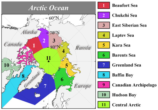
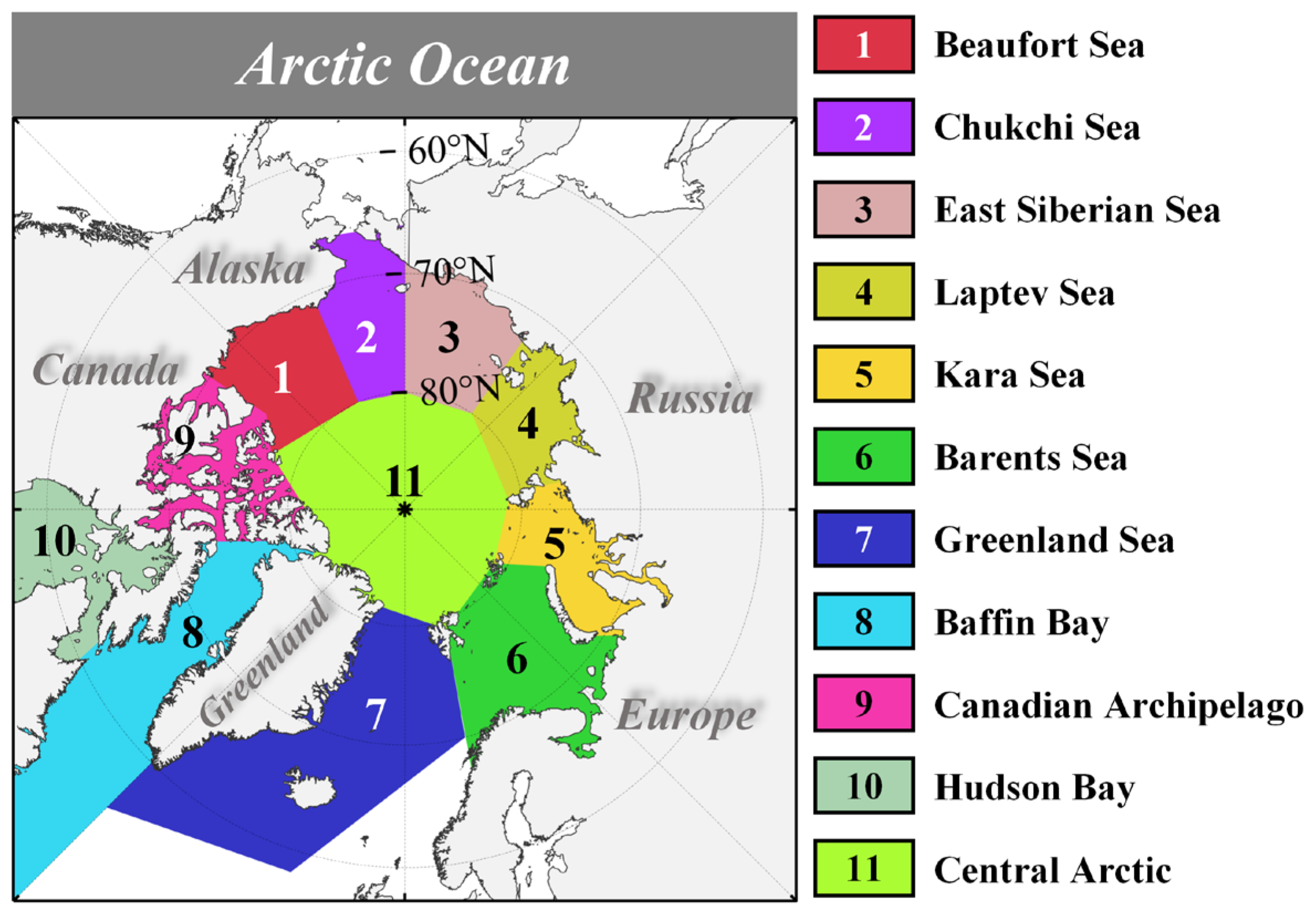
As shown in Figure 1, our study area is located in the Arctic Ocean, covering a wide range of seas from Greenland to the coast of Siberia, as well as around the Canadian Arctic Archipelago and Alaska. The pan-Arctic is a primary distribution area for global sea ice and one of the regions most significantly affected by climate change [35,36]. The evolution of Arctic sea ice in different sub-regions shows strong spatiotemporal heterogeneity [37,38], particularly with respect to ice extent and thickness.

Figure 1. Study area and sub-region division of the Arctic Ocean. The sub-region boundaries adopt the NSIDC gridded sea ice region codes (https://doi.org/10.5281/zenodo.12158836). The asterisk (*) marks the North Pole (90°N).

2.2. Training and Inference Data

We divide the input datasets into two categories according to model application scenarios: training datasets used for parameter optimization, and inference datasets adopted for final pan-Arctic sea ice thickness reconstruction. The predictor combinations differ between the two stages to balance training stability and observational constraint capability. To standardize spatial resolution across all predictors for ICE-3D modeling, we regrid every dataset involved in both training and inference onto the National Snow and Ice Data Center (NSIDC) polar stereographic grid. This grid features a horizontal resolution of 25 × 25 km with dimensions of 448 × 304 grid cells. All datasets adopted in this study are publicly available open resources. Detailed information for all datasets is summarized in Table 1.

Table 1. Overview of the datasets used for training and inference.

Dataset	Variables	Spatial Resolution	Temporal Resolution	Grid Projection	Time Span	Usage Stage
PIOMAS	SIT, SIC	~22 km	Daily	Generalized curvilinear	1979–2023	Training only
ERA5	SLP, T2M, U10, V10, SST	25 km	Daily	Regular	1979–2023	Training & Inference
NSIDC	SIC	25 km	Daily	Polar stereographic	1979–2023	Inference only
NOAA OISST	SST	25 km	Daily	Regular	1979–2023	Inference only

2.2.1. Training Datasets

During the training phase, Pan-Arctic Ice Ocean Modeling and Assimilation System (PIOMAS) reanalysis outputs serve as the core data source. The PIOMAS coupled ice–ocean system assimilates multi-source sea ice and ocean observations and provides consistent long-term physical fields of SIC and SIT [39]. Here, PIOMAS SIT is assigned as the regression target label for ICE-3D training, and PIOMAS SIC is adopted as the ice-related predictor.

Atmospheric forcing fields are derived from ERA5 fifth-generation ECMWF global atmospheric reanalysis [40]. The original hourly ERA5 outputs are averaged into daily values. Four variables are selected as model inputs: mean sea level pressure (SLP), 2 m air temperature (T2M), zonal 10 m wind (U10) and meridional 10 m wind (V10). Notably, ERA5 also provides pan-Arctic sea surface temperature (SST) that reflects upper ocean thermodynamic conditions with complete temporal coverage.

2.2.2. Inference Datasets

During the inference phase, we substitute PIOMAS reanalysis-derived predictors with satellite products to constrain the model using real remote sensing observations. We employ the merged gridded SIC dataset provided by the NSIDC, covering a 45-year period from 1979 to 2023. The NSIDC SIC dataset incorporates daily SIC observations from the Nimbus 7 Scanning Multi-channel Microwave Radiometer (SMMR), as well as the Special Sensor Microwave Imager (SSM/I) and Special Sensor Microwave Imager/Sounder (SSMIS) onboard the Defense Meteorological Satellite Program (DMSP) satellites. Please note that the NSIDC SIC dataset used here is a merged multi-satellite climate data record rather than independent raw observations from each sensor.

We also employ the Optimal Interpolated Daily Sea Surface Temperature (OISST) product provided by National Oceanic and Atmospheric Administration (NOAA), which integrates observations from various platforms (e.g., satellites, ships and Argo floats) into a regular global grid. The OISST product has been widely used in climate studies [41]. The version of OISST used in this study is mainly provided by the Advanced Very High Resolution Radiometer (AVHRR) with a spatial resolution of 1/4°.

2.3. Reference Data

The SMOS L-band brightness temperature data enable thin-ice (<1 m) thickness estimation [42], whereas CryoSat-2 is suited for thicker ice (>1 m) [18]. These complementary datasets are merged in the CS2SMOS product, which combines weekly averaged CryoSat-2 records with temporally matched SMOS data. However, this merged product is limited to winter observations. To assess summer thickness reconstruction accuracy, we employ a year-round satellite sea-ice thickness record from CryoSat-2. It provides a biweekly product with a grid resolution of 80 km, covering October 2010 to July 2020 [22].

We also employ upward-looking sonar (ULS) records from the Beaufort Gyre Exploration Project (BGEP), operational since 2003 [43]. Ice draft measurements obtained through this program are converted to thickness values via a 1.1 scaling coefficient [44], without compensating for snow cover or ice type variations. The three moorings carry official fixed site identifiers designated by BGEP: BGEP_A, BGEP_B, and BGEP_D. These stations deliver continuous, year-round SIT time series and perform well in capturing summer melting features. The three labels are consistently adopted hereafter to mark individual mooring sites and are visualized in Section 4.3.3 for comparison validation. Collectively, these BGEP mooring measurements serve as the primary in situ SIT benchmark observations used in our validation experiments.

The resolution of the above reference data is very limited. To address multiscale evolution comparisons, we employ the TOPAZ4 product, released by the Copernicus Marine Environment Monitoring Service (CMEMS), as a new reference. The TOPAZ4 is a coupled ocean–sea ice model with an advanced data assimilation system for the North Atlantic Ocean and Arctic [45]. The resolution of the TOPAZ4 model grid is 1/8°. The CS2SMOS ice thickness [18] is assimilated into the TOPAZ4 reanalysis SIT product during wintertime.

3. Methods

3.1. Data Preparation

Well-calibrated official datasets eliminate extra denoising and calibration work. We first regrid PIOMAS and ERA5 reanalysis outputs onto the NSIDC 25 km polar stereographic grid detailed in Section 2.2 to unify spatial resolution for rolling training and inference. Next, we assemble the tailored training dataset for ICE-3D. Since the raw grids contain numerous terrestrial and open-water invalid pixels, we generate an ice mask using SIC thresholds to exclude all non-ice grid entries from atmospheric and sea ice variables. Each sample is indexed by geographic coordinates and timestamp for convenient storage and retrieval. To mitigate parameter bias induced by uneven input data distributions, all variables are individually standardized via z-score transformation; this identical normalization pipeline is consistently applied throughout the inference stage.

All input predictors are processed using z-score normalization. The mean and standard deviation are calculated solely from the training data, and the same transformation coefficients are applied to the validation and test subsets to prevent information leakage. Grid cells with daily SIC > 0.15 are identified as ice-covered points and retained for SIT estimation; land and open-water grids below this threshold are masked. The three SST predictive metrics comprise domain mean, maximum, and minimum SST, which are computed only for ice-free ocean grids located north of 45°N.

3.2. ICE-3D Inference Framework

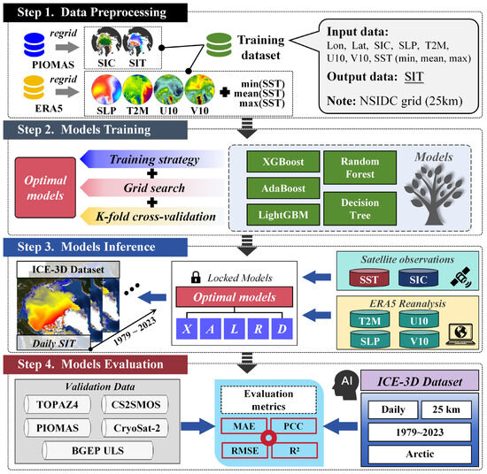
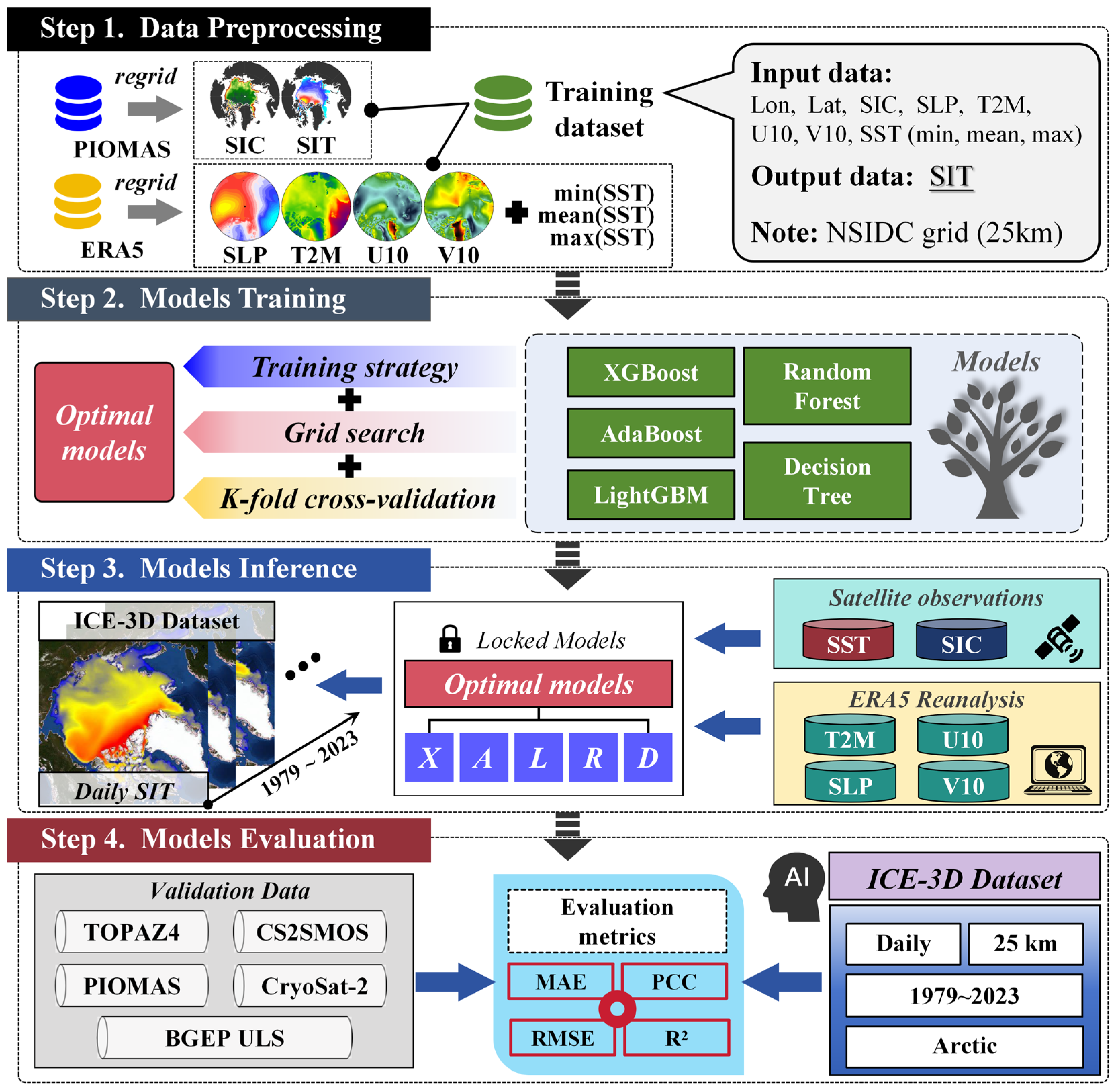
ICE-3D signifies the vertical three-dimensional structure of sea ice, aligning with multi-layer sea ice schemes in thermodynamic models and emphasizing the prospect of using reconstructed SIT as pseudo-observations to constrain coupled ice–ocean models in data assimilation. As shown in Figure 2, the ICE-3D framework adopts a modular design and is divided into four parts. To speed up the experimental process, we directly use the processed data for training and inference. In the modeling phase, we employed five types of ML models: Extreme Gradient Boosting (XGBoost), AdaBoost, Light Gradient Boosting Machine (LightGBM), RandomForest and DecisionTree.

Figure 2. Workflow schematic of the ICE-3D framework. ICE-3D sequentially implements four core modules: data preprocessing, model training, model inference, and model evaluation. Step 1 performs regridding and dataset assembly. Step 2 conducts grid search hyperparameter tuning and K-fold cross-validation, and selects optimal models. Step 3 applies the locked optimal models to generate daily pan-Arctic SIT. Step 4 evaluates model outputs against independent reference datasets.

The DecisionTree framework operates as a hierarchical supervised learning model extensively employed for forecasting applications. It efficiently extracts critical predictive variables from organized datasets through interpretable branching logic, demonstrating superior clarity compared to opaque neural networks. However, its simplified architecture struggles to process sophisticated spatiotemporal patterns [46]. RandomForest employs collective intelligence by integrating numerous tree-based classifiers to boost predictive robustness. Utilizing bootstrap sampling, constituent trees develop from varied data subsets with randomly chosen attributes during node construction. This approach amplifies model heterogeneity, suppresses overfitting and strengthens extrapolation potential through coordinated arboreal interactions [47]. XGBoost implements gradient enhancement by refining tree contributions through error gradient optimization while embedding stability constraints [48]. XGBoost achieves remarkable efficiency in handling large-scale datasets, but it requires precise configuration adjustments and involves resource-intensive computational workflows. LightGBM is also an ensemble learning method based on the gradient boosting algorithm [49], but it uses a leaf-wise decision tree structure (contrasting with level-wise expansion). It employs a histogram optimization algorithm rather than a traditional sorting method. However, reduced efficacy is observed when handling limited small samples or unbalanced distributions. AdaBoost is an innovative boosting algorithm that iteratively trains a series of weak learners to create a more powerful model [50]. The learning strategy of AdaBoost is to dynamically adjust the model weights, and it assigns higher weights to samples that were incorrectly predicted in the previous round. The final prediction integrates component models via a weighting scheme, enabling superior collective performance compared to individual weak learners (Text S1 in the Supplementary Materials).

As shown in Figure 2, in the inference phase (Step 3), satellite observations from NSIDC and OISST will replace the reanalysis data used in training. The atmospheric variables will continue to employ ERA5 data in inference. The input variables include two geographic coordinates (longitude and latitude), four atmospheric variables (U10, V10, T2M and SLP), three satellite SST observation statistics, and satellite SIC. ICE-3D performs independent training and inference for each calendar day from 1979 to 2023 where complete input datasets are available. Once the real-time training is completed, the updated model parameters are directly used for online inference to generate the SIT analysis field.

3.3. Spatiotemporal Multiscale Training Strategy

3.3.1. Baseline Configuration and Online Few-Shot Learning Paradigm

During the model training phase, all five tree-based base learners are trained under identical data partitioning and validation configurations. A grid search combined with K-fold cross-validation is implemented to calibrate hyperparameters and assess model robustness. Targeting real-time Arctic SIT reconstruction amid rapidly shifting Arctic climate conditions, we develop a tailored online few-shot learning workflow framed around daily rolling training. This temporal paradigm strictly adheres to causal constraints, ensuring no future information contaminates historical training records during retrospective long-term reconstruction. For each target calendar day, training samples are exclusively constructed within the predefined temporal window range without reliance on extensive archived datasets, enabling stable model calibration using only data encapsulated within one complete multiscale window. All environmental forcing inputs, training labels, and reconstructed SIT outputs are unified at a daily temporal resolution to maintain consistent spatiotemporal sampling standards. This lightweight single-window training design serves as the pivotal prerequisite for our subsequent 45-year retrospective pan-Arctic SIT reconstruction.

3.3.2. Mathematical Definition of STMFW

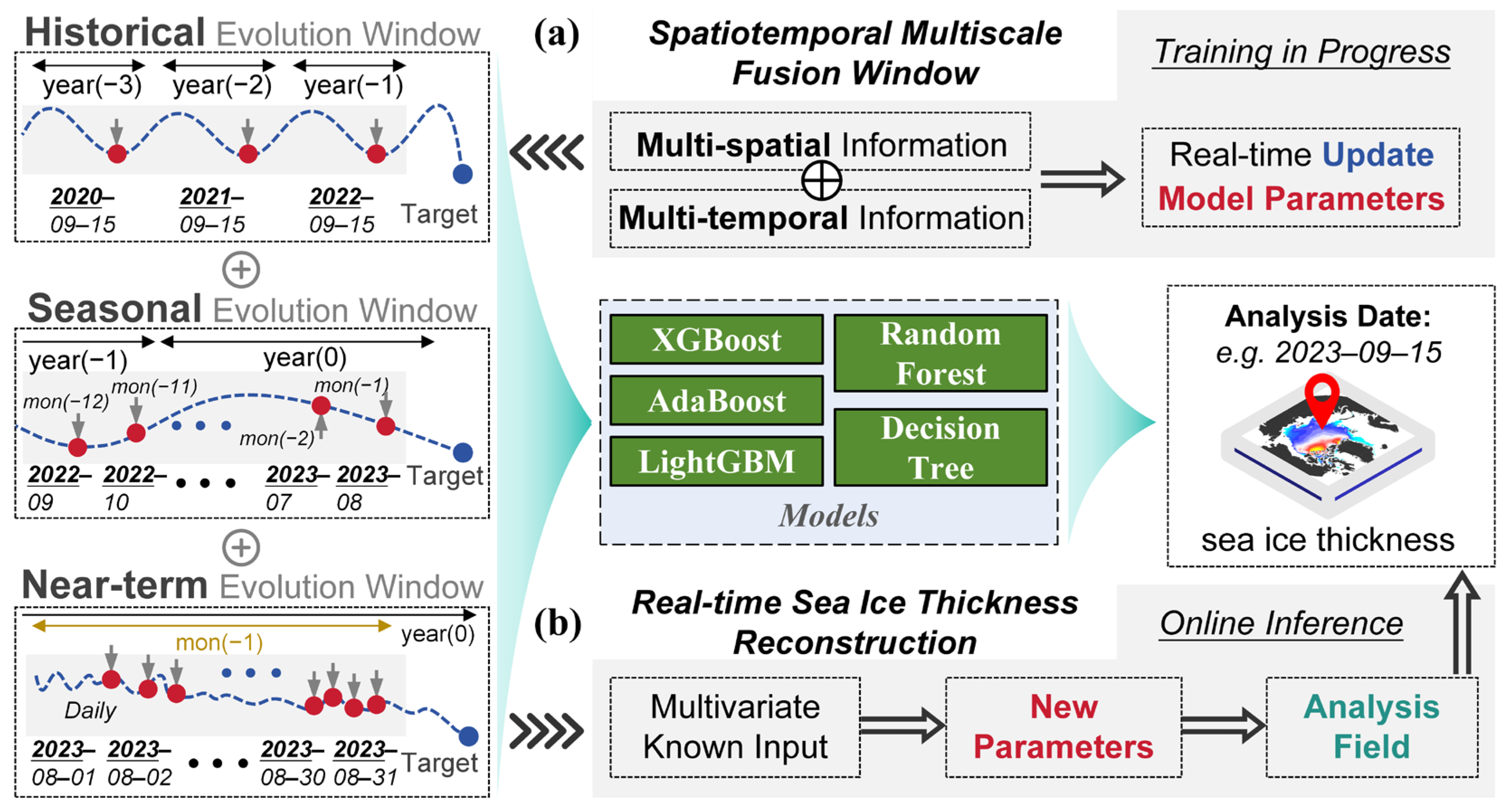
To balance training efficiency and sufficient extraction of sea ice evolutionary characteristics, we propose the Spatiotemporal Multiscale Fusion Window (STMFW), a customized online few-shot learning strategy tailored for Arctic SIT retrieval. STMFW aggregates three temporally nested windows that dominate Arctic sea ice variability across distinct timescales: the Historical Evolution Window (HEW), Seasonal Evolution Window (SEW), and Near-term Evolution Window (NEW), as illustrated in Figure 3. These complementary sampling windows separately decompose long-term interannual variability, annual seasonal freeze–melt cycles, and high-frequency short-term synoptic fluctuations. We denote the target prediction day as $t$, $T_{yr}=365$ days as the length of one annual cycle, and the pan-Arctic modeling domain as $\Omega$.

Figure 3. Schematic of the spatiotemporal multiscale fusion window (STMFW) framework for model training and online inference. (a) Architecture of STMFW, consisting of three complementary time-scale components: the Historical Evolution Window (HEW), Seasonal Evolution Window (SEW), and Near-term Evolution Window (NEW). Multiscale spatiotemporal features extracted from the three windows are fused and fed into multiple tree-based machine learning models. Model parameters are updated daily via incremental online few-shot learning. (b) Workflow of online inference. Using multivariate forcing inputs and newly updated model parameters, the framework generates gridded sea ice thickness analysis fields for the target date.

The Historical Evolution Window (HEW) is defined as:

$${\mathcal{W}}_{HEW}\left(t\right)=\{t-3T_{yr}, t-2T_{yr}, t-T_{yr}\}$$

(1)

which samples identical calendar dates across the preceding three years to resolve daily-scale interannual coupled ocean–atmosphere–sea ice signals.

The Seasonal Evolution Window (SEW) covers the previous 12 months with discrete monthly sampling to capture the periodic seasonal thermodynamic evolution of sea ice, formulated as:

$${\mathcal{W}}_{SEW}\left(t\right)=\{\tau \mid t-360\le \tau <t, \tau \in monthly interval\}$$

(2)

The Near-term Evolution Window (NEW) adopts consecutive daily sampling over the most recent 30 days to capture abrupt, nonlinear, short-term sea ice variations:

$${\mathcal{W}}_{NEW}\left(t\right)=\{\tau \mid t-30\le \tau <t, \tau \in daily interval\}$$

(3)

where window durations are finalized based on the intrinsic variability timescales of Arctic sea ice and preliminary sensitivity experiments, balancing reconstruction accuracy and computational expenditure.

3.3.3. Multiscale Feature Concatenation and Fusion

For any grid point $\mathit{x}\in \Omega$ within the modeling domain, multivariate environmental predictor sequences extracted from each temporal window are denoted ${\mathbf{F}}_{HEW}(\mathit{x},t)$, ${\mathbf{F}}_{SEW}(\mathit{x},t)$, and ${\mathbf{F}}_{NEW}(\mathit{x},t)$, incorporating SIC, atmospheric forcing variables, and ice-free SST spatial statistics. These multiscale feature sequences are concatenated along the feature dimension to construct the unified model training datasets:

$${\mathbf{F}}_{total}(\mathit{x},t)=Concat({\mathbf{F}}_{HEW},{\mathbf{F}}_{SEW},{\mathbf{F}}_{NEW})$$

(4)

No manual weighting coefficients are assigned to individual windows; tree-based ensemble models adaptively learn the relative contribution of long-term, seasonal, and short-term spatiotemporal signals throughout the training process. Ablation tests presented in Figure S2 verify that the full three-window configuration delivers optimal reconstruction performance, confirming that HEW, SEW, and NEW capture mutually exclusive and complementary sea ice evolutionary information, and validating the rationality of the STMFW framework.

3.3.4. Daily Incremental Parameter Updating and Online Inference

Instead of exhaustive full retraining, incremental fine-tuning is performed daily upon the arrival of new STMFW samples to alleviate the computational burden. The online parameter updating process is optimized via the regression loss function:

$${\Theta }_t=\arg \underset{\theta }{\min }\mathcal{L}\left(y\right(\mathit{x},t),\mathcal{M}({\mathbf{F}}_{total}(\mathit{x},t);{\Theta }_{t-1}\left)\right)$$

(5)

where ${\Theta }_{t-1}$ represents inherited model parameters from the previous day, ${\Theta }_t$ denotes updated parameters for the target day t, $\mathcal{M}(\cdot )$ stands for the tree-based ensemble regression model, and $\mathcal{L}$ is the loss function for SIT retrieval. The refined parameters are subsequently applied for online inference to generate gridded pan-Arctic SIT fields:

$$\widehat{y}(\mathit{x},t)=\mathcal{M}\left({\mathbf{F}}_{total}\right(\mathit{x},t);{\Theta }_t)$$

(6)

While STMFW expands the feature space and brings mild computational overhead relative to conventional single-scale sliding windows, incremental online updating substantially offsets this cost. Benefiting from the online few-shot attribute of STMFW, the model can be trained effectively using only data within a single temporal window, which eliminates dependence on massive long-term continuous training datasets and enables our multi-decadal historical SIT reconstruction. To clarify operational feasibility, Text S2 in the Supplementary Materials provides a formal definition and operational details. In addition, an analysis of the usability and stability of ICE-3D in scenarios where parameter updates are unavailable is shown in Figure S4.

3.3.5. Definition of Core Innovation Boundary

The spatiotemporal multiscale perception learning proposed herein originates entirely from the multi-timescale sampling and fusion mechanism embedded within STMFW, rather than inherent characteristics of the tree-based base learners themselves. Tree ensemble algorithms and conventional single-scale sliding window sampling are mature techniques widely adopted in existing studies. Accordingly, multiple tree-based models are adopted in our experiments not for simply selecting a superior individual learner, but to validate the universal effectiveness and generalization of the proposed STMFW strategy across diverse baseline architectures. The primary innovation of the ICE-3D framework centers on the customized STMFW online few-shot learning strategy, which fuses multi-timescale sea ice evolution signals to disentangle cross-scale nonlinear covariations between SIT and other predictors. Enabled by this multiscale fusion paradigm, ICE-3D achieves stable year-round pan-Arctic SIT reconstruction and yields pronounced accuracy improvements for summer SIT under sparse observational constraints. It should be noted that Figure 2 and Figure 3 only illustrate the general ICE-3D workflow and STMFW schematic mechanism and do not restrict the evaluation time range.

3.4. Evaluation Metrics

Four performance metrics—coefficient of determination (R²), Pearson correlation coefficient (PCC), mean absolute error (MAE) and root mean square error (RMSE)—are selected to evaluate the performance of ICE-3D. All metrics are calculated based on valid ice grid points, which are selected based on SIC values, using statistics from reference (Ref) and inference (Inf). R² represents the proportion of variance in Ref explained by Inf, providing an indication of the goodness-of-fit. PCC measures the linear correlation between Inf and Ref, with values ranging from −1 to 1. MAE and RMSE quantify the absolute and relative errors between Inf and Ref, respectively.

$$R^2=1-\left({\displaystyle \frac{{\sum }_{i=1}^n{\left(Re{f}_i-In{f}_i\right)}^2}{{\sum }_{i=1}^n{\left(Re{f}_i-\overline{Ref}\right)}^2}}\right)$$

(7)

$$PCC={\displaystyle \frac{{\sum }_{i=1}^n\left(Re{f}_i-\overline{Ref}\right)\left(In{f}_i-\overline{Inf}\right)}{\sqrt{{\sum }_{i=1}^n{\left(Re{f}_i-\overline{Ref}\right)}^2{\left(In{f}_i-\overline{Inf}\right)}^2}}}$$

(8)

$$MAE={\displaystyle \frac{1}{n}}{\sum }_{i=1}^n\left|Re{f}_i-In{f}_i\right|$$

(9)

$$RMSE=\sqrt{{\displaystyle \frac{1}{n}}{\sum }_{i=1}^n{\left(Re{f}_i-In{f}_i\right)}^2}$$

(10)

4. Results

4.1. Overall Performance Evaluation

We create the experimental environment using Python 3.9 and the scikit-learn machine learning framework [51]. Training and inference are conducted on a personal workstation with an NVIDIA GeForce RTX V100 GPU with 16 GB of memory. It is worth mentioning that after completing the hyper-parameter tuning, the model settings of ICE-3D no longer require any modification, which saves additional training time (for more details, see Text S3 in the Supplementary Materials).

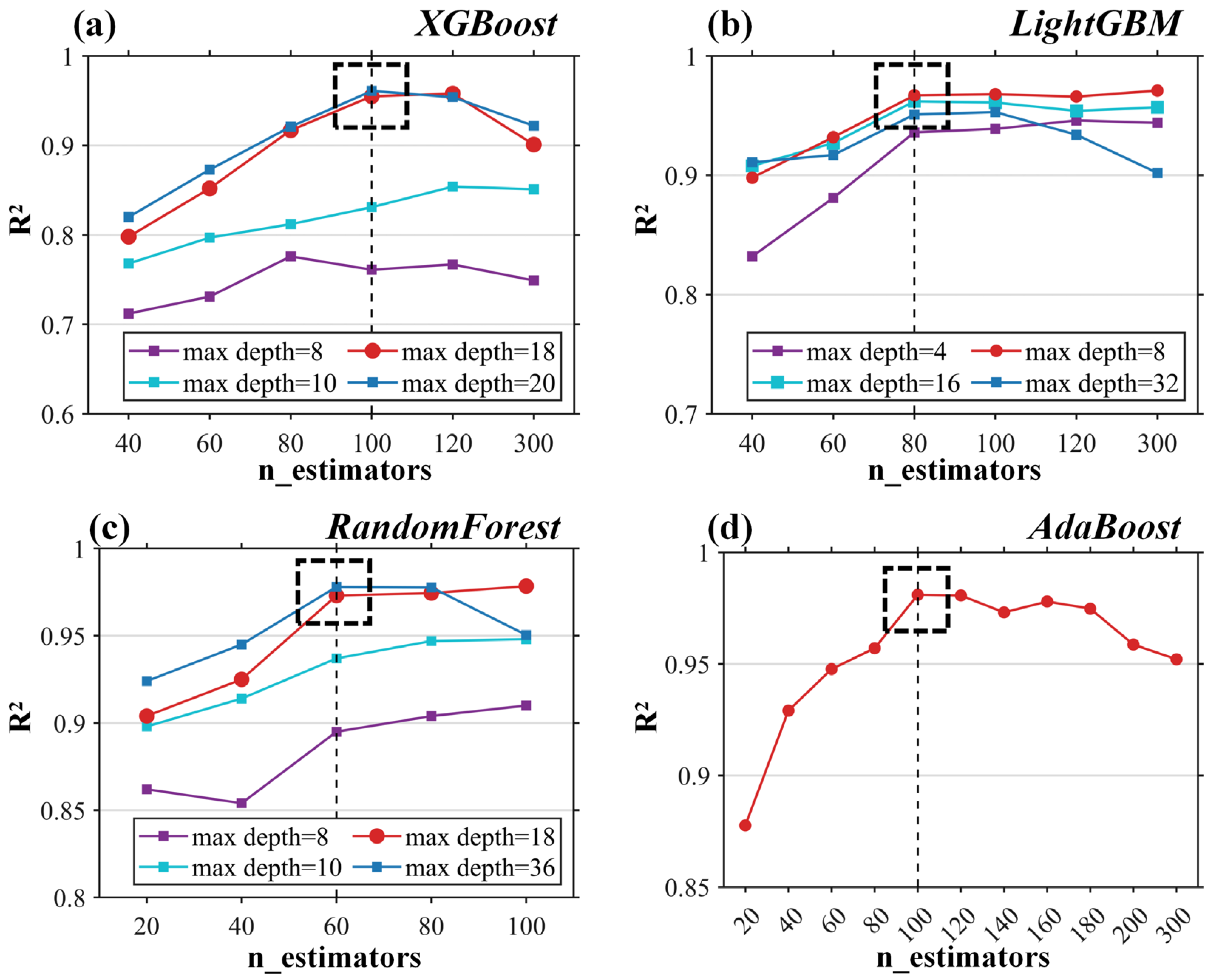
In decision tree-based models, there are two core hyper-parameters, n_estimators and max_depth. n_estimators represents the number of decision trees in the model and max_depth controls the maximum depth of the tree. Generally, increasing n_estimators will improve the learning ability of the model and reduce the risk of overfitting. When max_depth is too large, the model will overfit, while if max_depth is too small, it may lead to underfitting. The advantage of AdaBoost is that it integrates multiple weak learners to improve model performance, so max_depth defaults to 1. It should be noted that the DecisionTree has only one tree, so there is no need to tune n_estimators. Other parameters are usually set to default values because they have little impact. A standalone single Decision Tree is deliberately incorporated as the simplest baseline benchmark for controlled comparison. Since Random Forest is built upon the bagging ensemble of numerous independent single decision trees, this pairwise comparison enables us to explicitly quantify the predictive performance enhancement exclusively derived from the bagging ensemble strategy, which separates the fitting capacity of an individual tree from the benefits brought by multi-tree ensemble integration.

The optimal parameters for each model are shown in Table S1, and we select the parameter combination with the highest score (Figure 4) as the hyper-parameters for ICE-3D. In the retrospective inference, the best model is AdaBoost, followed by LightGBM and RandomForest. It is reasonable that DecisionTree, as the basic structure of other models, performs the worst. Overall, the parameters after grid search make the ICE-3D reach a relatively stable level. The STMFW training strategy we proposed enables different ML models to be fully trained. We can observe that the inference results of all models can basically explain more than 93% of the variance of SIT, and their MAE values are also around 0.1 m. Feature importance provides preliminary criteria for explaining the stability and effectiveness of the ICE-3D. All input features play an important role. For more details on feature importance, see Text S1 and Figure S1. Feature importance analysis reveals that SIC and atmospheric variables dominate SIT estimation. Geographic coordinates and lagged sea ice evolution signals also provide non-negligible predictive information.

Figure 4. Hyperparameter sensitivity analysis of four ensemble machine learning models adopted within the ICE-3D framework. Subpanels (a–d) illustrate variations in the ${\mathrm{R}}^2$ against the number of base estimators (n_estimators) under different settings of maximum tree depth (max_depth) for XGBoost, LightGBM, Random Forest and AdaBoost, respectively. Black dashed rectangles denote the optimal hyperparameter combination identified for each model. All sensitivity experiments adopt identical preprocessing pipelines and share the same training and testing samples. This analysis also identifies the overfitting threshold for each model.

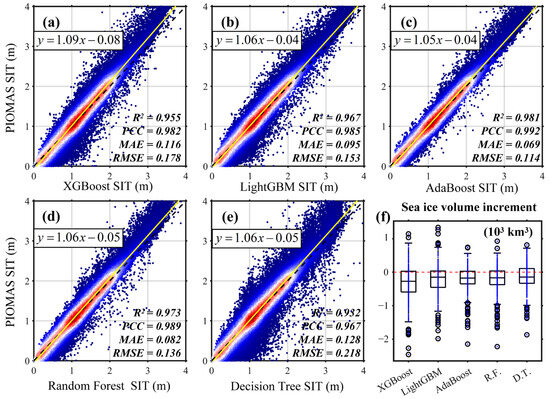
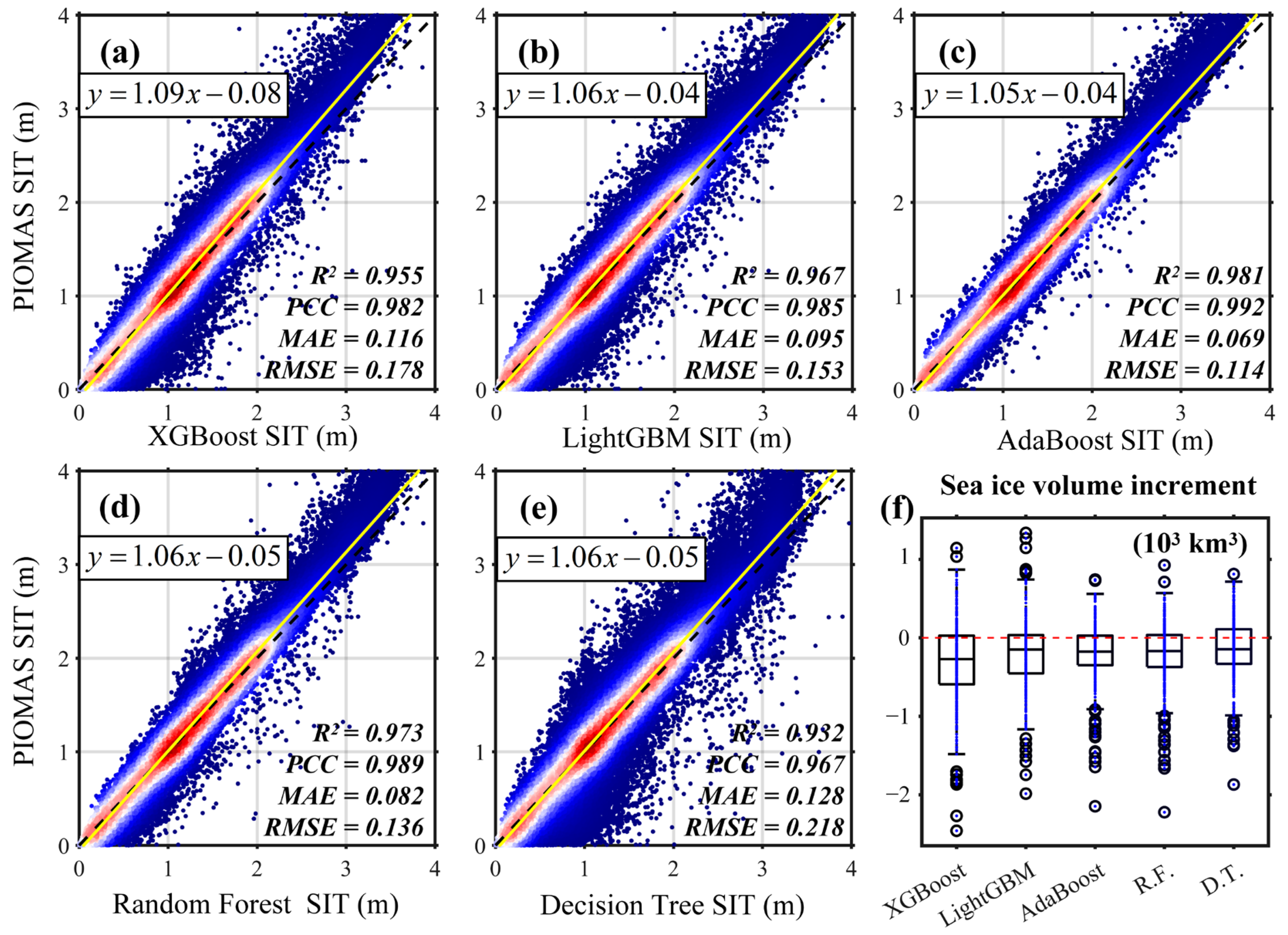
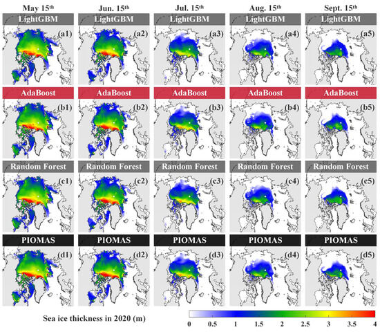
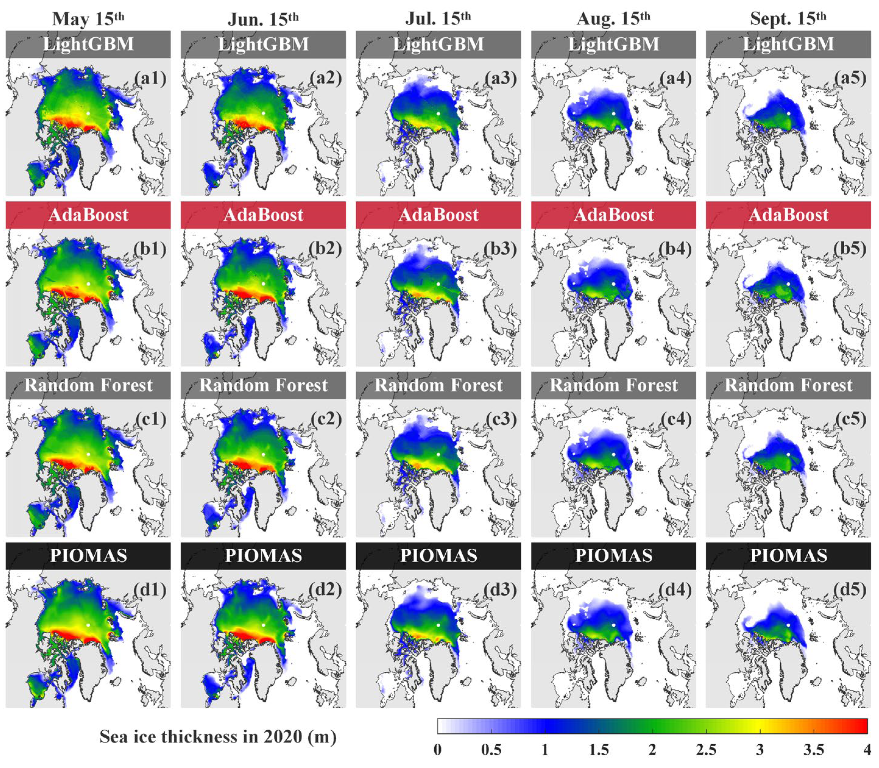
AdaBoost outperforms other models and exhibits smaller uncertainty. We can observe that ICE-3D has better inference capability for sea ice in the 1–2 m range, which is due to the larger quantity of sea ice in this range. Moreover, the estimation bias of AdaBoost is significantly smaller (Figure 5c). In the comparison of SIV increments, all models show consistent negative deviations relative to PIOMAS, which means that the ICE-3D inference tends to believe that the sea ice is thinning overall, which is indeed the case [52]. Figure 6 shows the spatial distribution of ICE-3D. The sea ice melt process from May to September 2020 is accurately captured, particularly the spatial patterns of thin and thick ice. ICE-3D effectively generates the basic spatial configuration of SIT, indicating that the inference scheme is valid. ICE-3D shows sufficient application flexibility, which indicates its suitability for estimating Arctic SIT.

Figure 5. Comparison of daily SIT estimated by five machine learning modules of ICE-3D against PIOMAS reference SIT. Panels (a–e) show density scatter plots for XGBoost, LightGBM, AdaBoost, Random Forest (R.F.), and Decision Tree (D.T.), respectively. The black dashed line indicates the 1:1 perfect agreement line, and the solid yellow line represents the linear regression fit between model predictions and PIOMAS SIT. Statistical metrics including ${\mathrm{R}}^2$, PCC, MAE, and RMSE are labeled in each subpanel. Panel (f) presents boxplots of daily SIV increment, defined as model-inferred SIV minus PIOMAS reference SIV (units: $10^3 \mathrm{k}{\mathrm{m}}^3$).

Figure 6. Comparison of the three optimal models in (a1–c5) ICE-3D with (d1–d5) PIOMAS. (1–5) represent the May–September 2020 SIT samples.

It should be emphasized that the PIOMAS-based evaluation in this subsection only reflects the model’s capability to reproduce the training target dataset and serves as an intra-dataset fitting assessment, rather than absolute accuracy validation against real independent observations (Figure 5). Rigorous out-of-sample generalization evaluation is independently implemented in Section 4.3 using unused satellite and in situ measurements, forming a two-stage progressive validation framework. ICE-3D adopts a strict daily rolling online learning paradigm via the STMFW strategy, where training and inference are stepwise and temporally independent for each target day across the full 1979–2023 period. Figure 6 presents hyperparameter sensitivity tests for model optimization. The 2020 results displayed here are used only as a representative case for hyperparameter screening and preliminary model assessment, rather than selectively chosen favorable outputs. All annual reconstructions follow exactly the same rolling inference pipeline, and stable multi-year performance across the entire study period is fully demonstrated in Figure 7 and Figure 8. This full-cycle comparison consistently further validates that AdaBoost can achieve optimal and stable SIT estimation performance, which supports our final model selection.

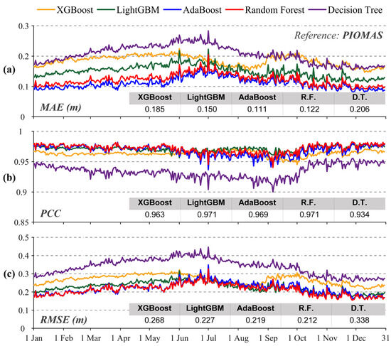
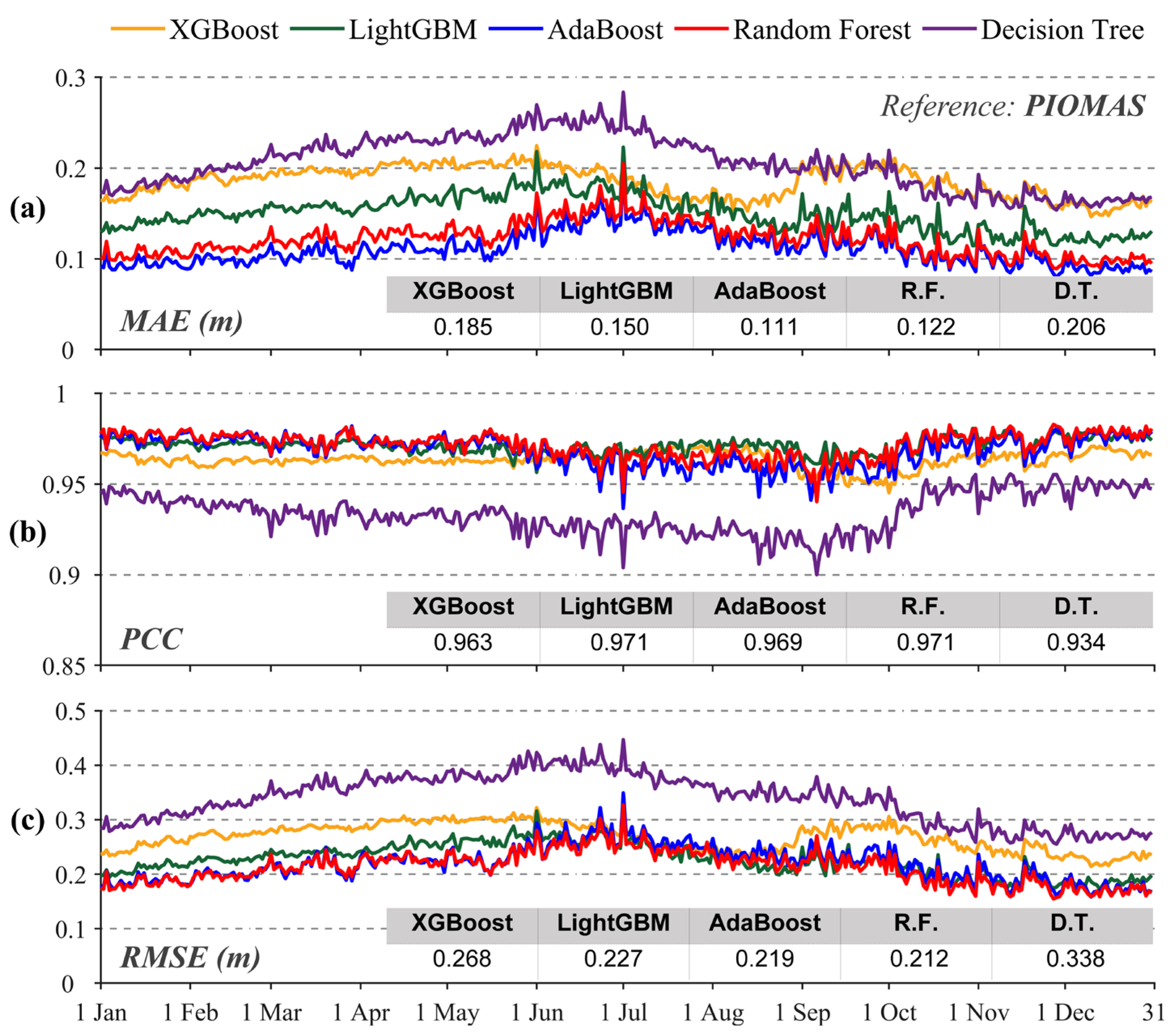
Figure 7. Comparison of the daily inference results of five ML models in ICE-3D applied to SIT from 1979 to 2023, validated against PIOMAS. The five models are XGBoost, LightGBM, AdaBoost, Random Forest (R.F.), and Decision Tree (D.T.). (a) MAE, (b) PCC, (c) RMSE. Tabulated values within each panel denote the time-averaged metric for each model.

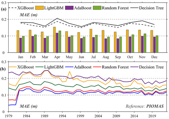
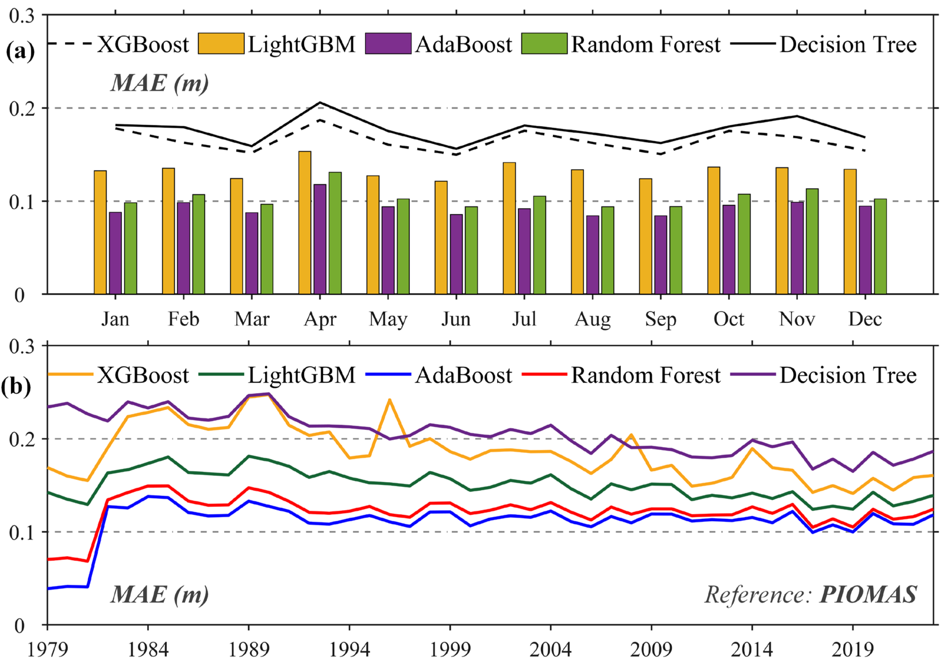
Figure 8. (a) Monthly average and (b) annual average MAE for ICE-3D.

4.2. Spatiotemporal Robustness Evaluation and Error Pattern Analysis

Building upon the preliminary model screening in Section 4.1, this section conducts comprehensive full-period and full-domain spatiotemporal robustness evaluation of the five ICE-3D model configurations. Multi-metric comparisons and systematic error pattern analysis are performed to quantitatively verify model stability and characterize reconstruction spatiotemporal uncertainty.

4.2.1. Temporal Robustness and Error Characteristics

Figure 7 shows a multi-metric comparison of the five models at the daily scale. The three metrics provide different perspectives on the stability of ICE-3D. Among these, AdaBoost performs the best, with the MAE ranging between 0.1 m and 0.15 m. The PCC of most models is around 0.95, and it shows a reasonable spatial distribution. The seasonal evolution of SIT has some impact on the inference of different models (Figure 8). XGBoost performs better than DecisionTree, but both have a significantly higher MAE compared to the other three models, especially in the starting months of Arctic sea ice melting (Apr.) and freezing (Nov.). It can be found that AdaBoost ranks first among all models with excellent stability, with an annual average MAE of less than 0.15 m. RandomForest is closest to the performance of AdaBoost with a slightly higher error. LightGBM has an annual average MAE of about 0.15 m (<0.2 m). Therefore, the inference results of AdaBoost are the best product of ICE-3D, which will be used in the following analysis. Note that the STMFW strategy requires a 3-year historical window for cold-start initialization. The inference outputs from this cold-start phase (Figure 8b) are not representative of stable long-term performance, owing to limited available training information and artificially suppressed errors. Thus, we exclude the cold-start period and adopt a unified analysis period starting from 1985 to guarantee objective evaluation.

4.2.2. Spatial Error Distribution and Regional Uncertainty Analysis

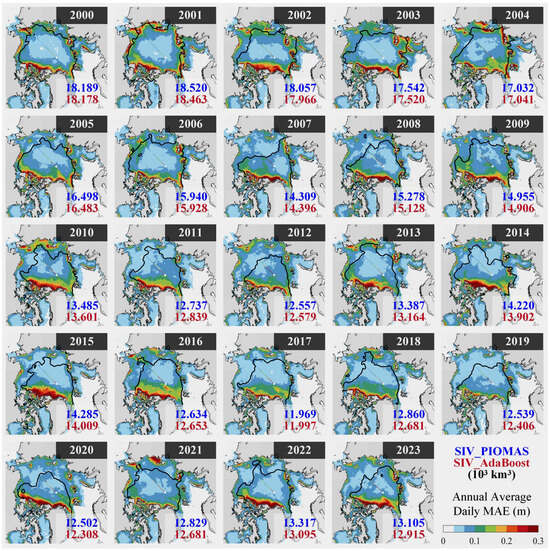
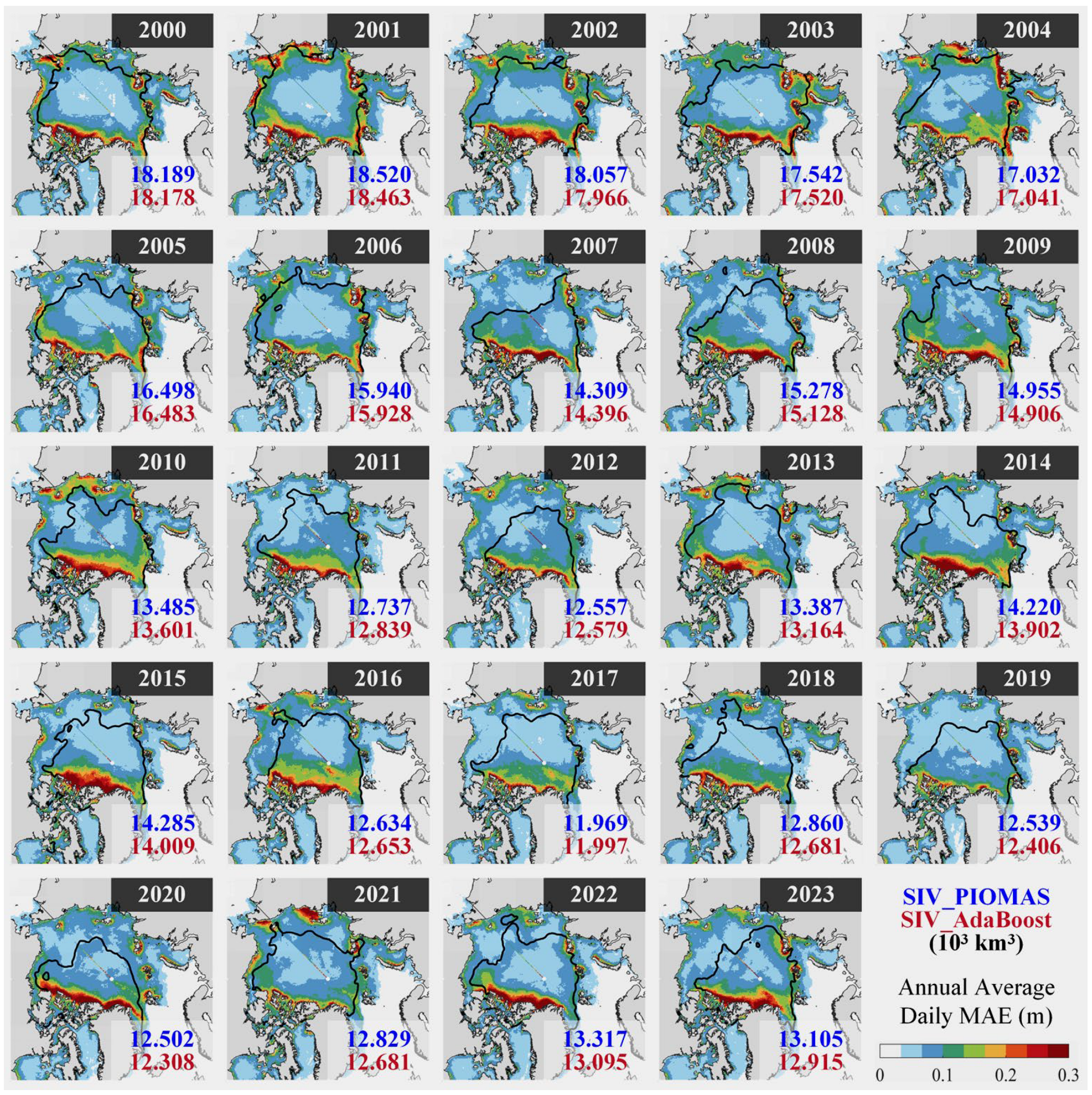
The distribution of the annual average spatial MAE from 2000 to 2023 is shown in Figure 9. The spatial MAE of SIT estimated by AdaBoost is almost always around 0.1 m. Among them, the areas with large errors are mainly distributed in the thick ice areas along the Canadian Arctic Archipelago and the coast of Greenland, with the maximum MAE exceeding 0.3 m. In addition, there are also large errors near the sea ice edge in September, which shows that the seasonal melting of sea ice has an impact on ICE-3D. Compared with ICE-3D, PIOMAS optimistically estimates the extent of SIV decline [53]. In fact, all ML models in ICE-3D tend to have larger SIV losses than PIOMAS. ICE-3D retains the spatial distribution of SIT learned from PIOMAS while correcting for regional differences when driven by satellite observations. Therefore, the temporal and spatial errors of ICE-3D are reasonable.

Figure 9. Spatial MAE distribution of SIT from 2000 to 2023. The solid black line represents the sea ice edge in September (SIC = 15%), and the numbers in the lower right corner represent the annual average SIVs of PIOMAS (blue) and AdaBoost (red).

Notably, higher MAE values are persistently distributed along the Greenland coastline and within the Canadian Arctic Archipelago. Such elevated uncertainties over these marginal zones can be attributed to two factors. First, intricate fjords and narrow channels generate small-scale, rapidly evolving coastal sea ice features that cannot be fully resolved on the 25 km grid. Second, available in situ and satellite SIT observations remain sparse within archipelagic waters, limiting the model’s ability to capture localized ice variability in these complex coastal domains.

4.3. Consistency Validation with Multi-Source Observations

To systematically verify the out-of-sample generalization capability of ICE-3D against independent observation constraints (distinct from PIOMAS-based intra-dataset evaluation in Section 4.1 and Section 4.2), this section conducts segmented validation grouped by observational datasets with complementary seasonal coverage and spatial–temporal features. Three independent sources are applied sequentially: winter satellite retrievals (CS2SMOS), summer satellite measurements (CryoSat-2), and long-term high-frequency in situ mooring records (BGEP ULS). This dataset-based framework accommodates the seasonal limitations, resolution discrepancies, and unique uncertainty features of each product, enabling comprehensive year-round verification across different timescales.

4.3.1. Winter Validation Against CS2SMOS Satellite SIT Product

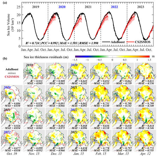
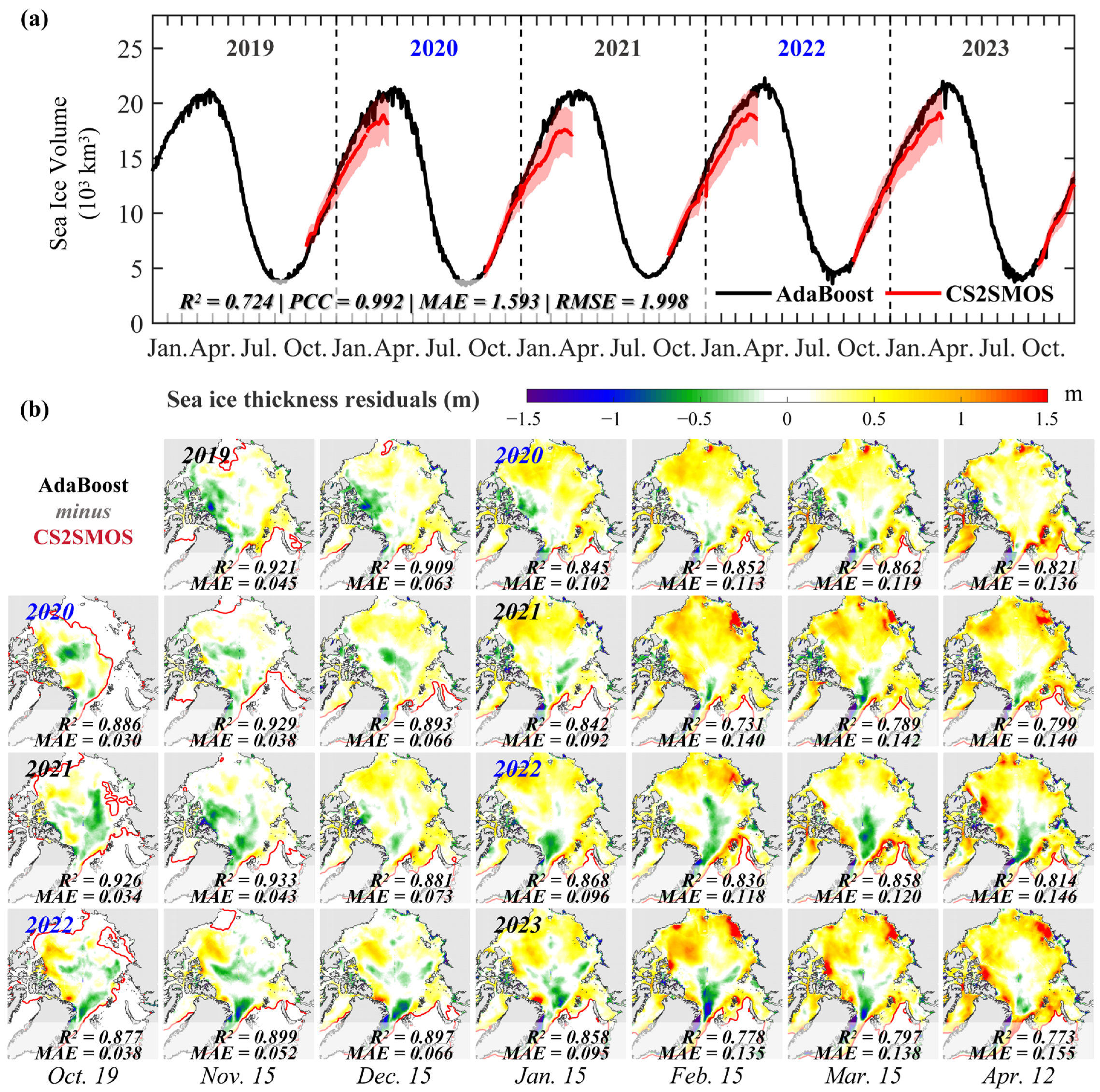
As shown in Figure 10, the CS2SMOS product can only be used to evaluate the winter SIT. Arctic sea ice extent and volume increase from October to April. ICE-3D shows reasonable seasonal evolution, which is consistent with the CS2SMOS. The SIV estimated by ICE-3D remains relatively stable, with an average MAE of 1.593 × 10³ km³ compared to CS2SMOS. The seasonal cycle of ICE-3D is highly correlated with CS2SMOS, especially in the early stage of sea ice freezing. The uncertainty of CS2SMOS gradually increases as the sea ice continues to freeze. ICE-3D can accurately capture the process of sea ice thickening from thin to thick. From February to April, ICE-3D overestimates the peak of SIV compared with CS2SMOS, but still remains within the uncertainty range.

Figure 10. Comparison of CS2SMOS with AdaBoost in ICE-3D. (a) SIV; (b) spatial distribution of SIT residuals (AdaBoost minus CS2SMOS). The red lines represent the sea ice edge.

The spatial anomaly distribution of ICE-3D relative to CS2SMOS is shown in Figure 10b. From October to January, most of the SIT anomalies range from −0.5 m to 0.5 m and the spatially averaged MAE is almost less than 0.1 m. The SIT anomalies from February to April show that a large number of positive anomalies are concentrated in the marginal areas, especially near the East Siberian Sea and the Canadian Arctic Archipelago, where the overestimation reaches more than 1.5 m. However, the SIT in the central Arctic is underestimated by only about 0.5 m. Therefore, the heterogeneity of this spatial anomaly distribution leads to a false overestimation of SIV by ICE-3D. The spatial distribution of ICE-3D is largely inherited from PIOMAS, which is inevitable in ML. Compared with CS2SMOS, the spatial average MAE of ICE-3D is less than 0.16 m, which can explain about 80% of the information in CS2SMOS. In summary, ICE-3D has good ability to generate winter SIT and is stable in capturing the evolution of winter SIV.

4.3.2. Summer Validation Against CryoSat-2 Satellite SIT Product

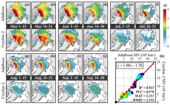
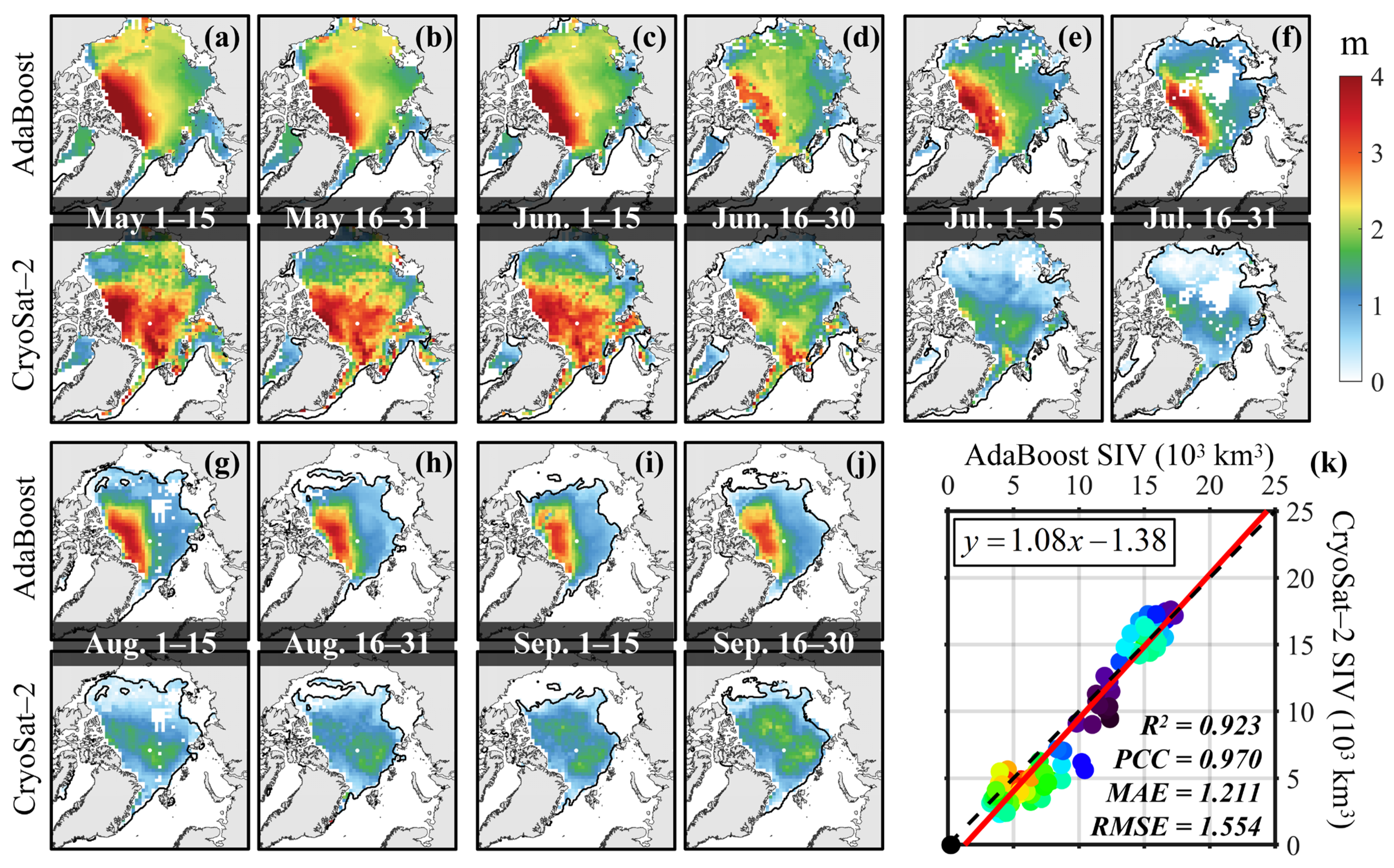
In addition to generating winter SIT, ICE-3D can also provide daily estimates of summer SIT when observations are missing. We employ biweekly CryoSat-2 data to assess summer SIT. The spatial distribution of SIT (Figure 11) from AdaBoost is similar to that of CryoSat-2. The distribution of thick ice (SIT > 3 m) estimated by AdaBoost is more concentrated, but the distribution of CryoSat-2 is more scattered. The process of sea ice melting can also be effectively captured by ICE-3D and the results of AdaBoost show reasonable range contraction and ice thickness reduction.

Figure 11. Comparison of CryoSat-2 with ICE-3D. (a–j) Spatial distribution of biweekly SIT from May to September 2015. (k) Comparison of AdaBoost and CryoSat-2 SIV from 2010 to 2020.

However, CryoSat-2 shows a more uniform distribution of SIT in the central Arctic. In fact, CryoSat-2 can capture a large portion of the interannual variability observed in existing SIT records [22], such as those from airborne electromagnetic (AEM), ULS and acoustic Doppler current profilers (ADCP) observations, but it still underestimates the roughest SIT [54] in coastal areas. The regions where CryoSat-2 underestimates SIT are primarily around the Canadian Arctic Archipelago and Greenland, but this bias can be corrected by ICE-3D. The PCC between the biweekly SIV from ICE-3D and CryoSat-2 reaches 0.97 (Figure 11), which indicates that while there are local differences in spatial patterns, the seasonal and interannual variations in SIV are relatively consistent.

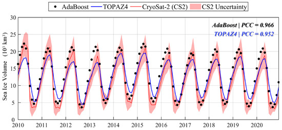
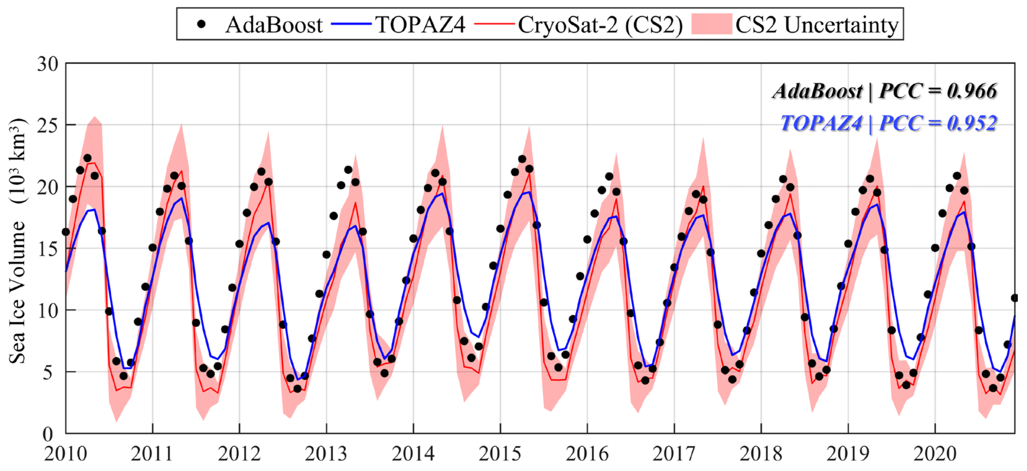
To further evaluate the accuracy of ICE-3D seasonal evolution, we compare the monthly average SIV from 2010 to 2020 (Figure 12). In comparison, AdaBoost in ICE-3D performs slightly better than TOPAZ4, especially in the melt season. TOPAZ4 assimilates CS2SMOS (winter only), so it is not surprising that its performance in winter is consistent with satellite observations. The ice growth rate in CS2SMOS is slower during the freezing season (Figure 10), so the SIV peak of TOPAZ4 is smaller than that of AdaBoost. In addition, the melting start date of TOPAZ4 is slightly later than that of AdaBoost, which leads to a smaller melting rate and an overestimation of SIT in September.

Figure 12. Time series comparison of monthly averaged SIV from 2010 to 2020.

4.3.3. Local Validation Against BGEP In Situ Mooring Observations

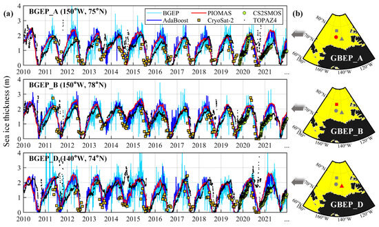
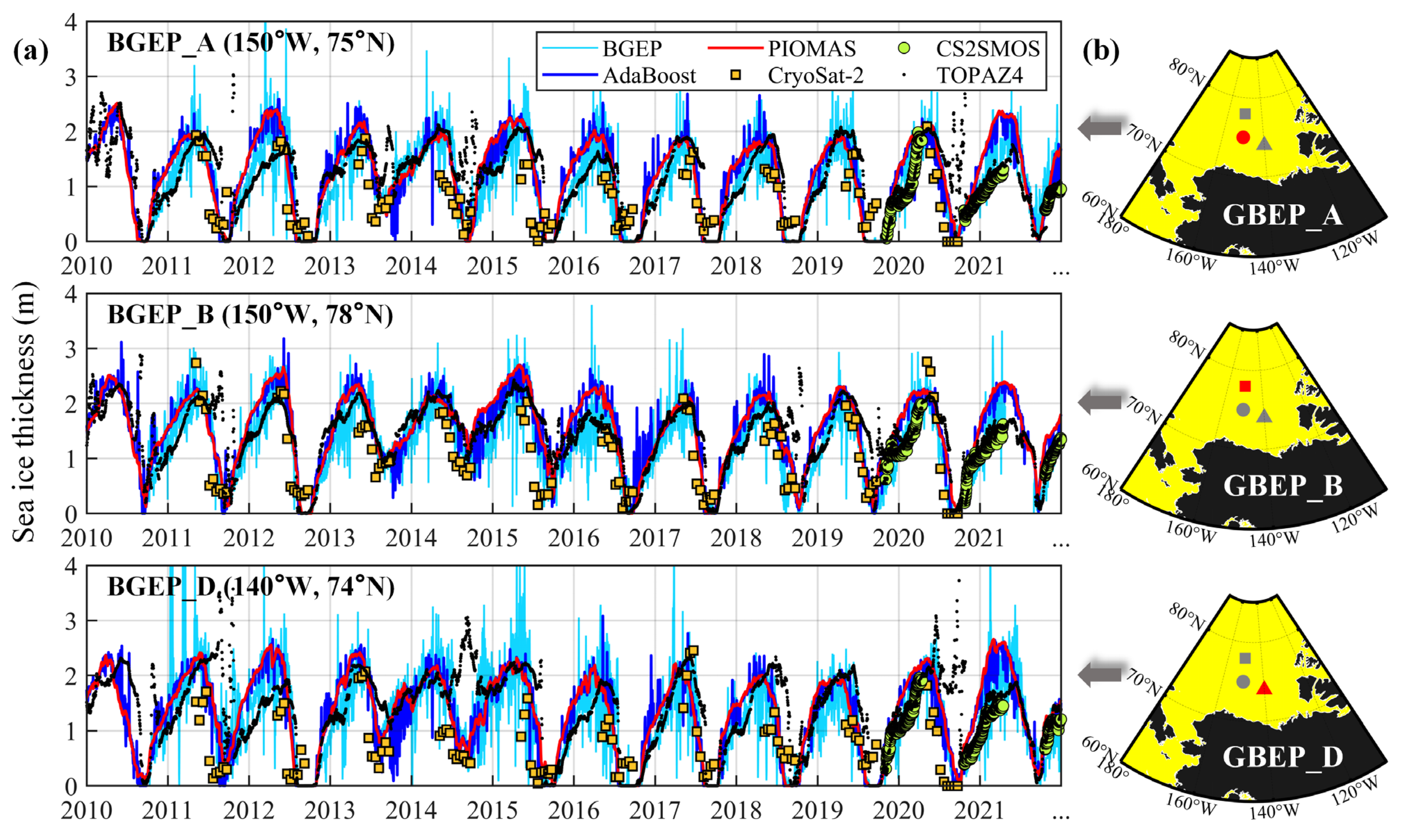
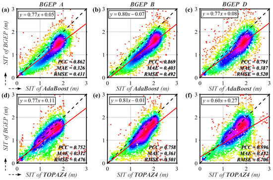
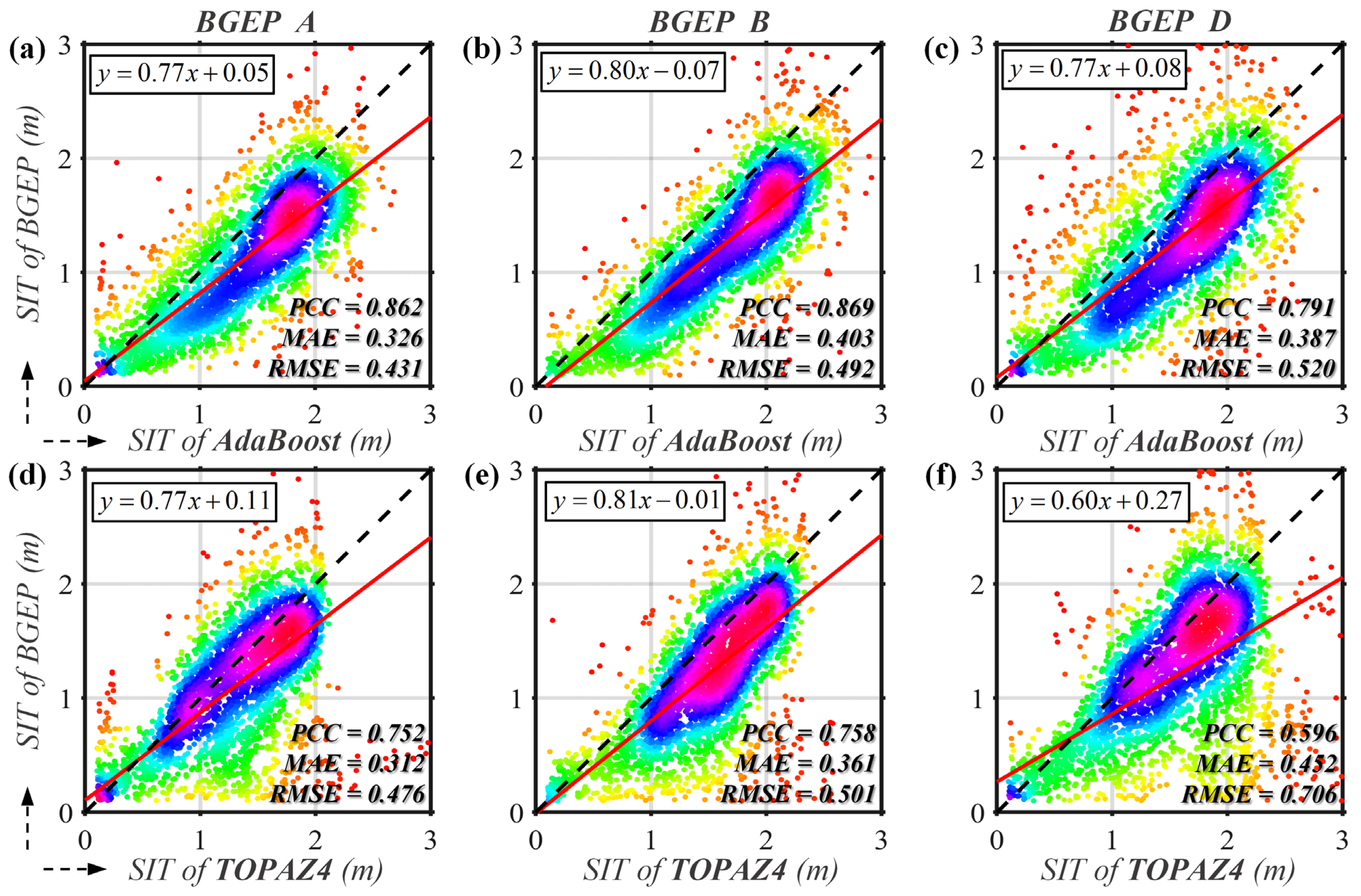
The spatial observation range of the ULS sensor on the BGEP mooring array is limited, but its high update frequency makes it suitable for long-term monitoring of local areas, revealing more detailed local information than satellite observations (Figure 13). There is no significant seasonal difference between CryoSat-2 and BGEP. However, the biweekly CryoSat-2 observations make it difficult to show more details. The reanalysis data have higher temporal and spatial resolution, but the SIT evolution of both PIOMAS and TOPAZ4 is relatively smooth. AdaBoost shows high-frequency nonlinear signals, which are more consistent with the in situ observations of BGEP. ICE-3D is driven by high-frequency atmospheric forcing and real remote sensing observations, which enables it to capture the strong nonlinear evolution. AdaBoost is closer to the observations at the three mooring points (Figure 14). TOPAZ4 obviously overestimates thin ice in the range of 0~1 m, with the local absolute error even exceeding 2 m. AdaBoost overestimates mainly thick ice (about 2 m), with a MAE of about 0.5 m. The above results indicate that ICE-3D performs excellently in SIT inference, with a significant advantage in capturing high frequency and strongly nonlinear evolution. At the same time, we acknowledge that the spatial representativeness of this summer validation is restricted by the limited coverage of CryoSat-2 and BGEP mooring data, and CryoSat-2 summer retrievals are affected by melt-pond-related uncertainties.

Figure 13. Comparison of SIT between ICE-3D and BGEP. (a) Time series of SIT (light blue) for three ULS moorings. (b) Location markers of BGEP_A, BGEP_B and BGEP_D.

Figure 14. Comparison of BGEP data from 2010 to 2021 with (a–c) AdaBoost and (d–f) TOPAZ4. The solid red line represents the linear best fit.

5. Discussion

5.1. Seasonal Variability of Arctic SIT

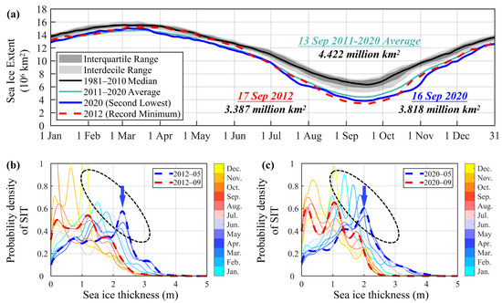
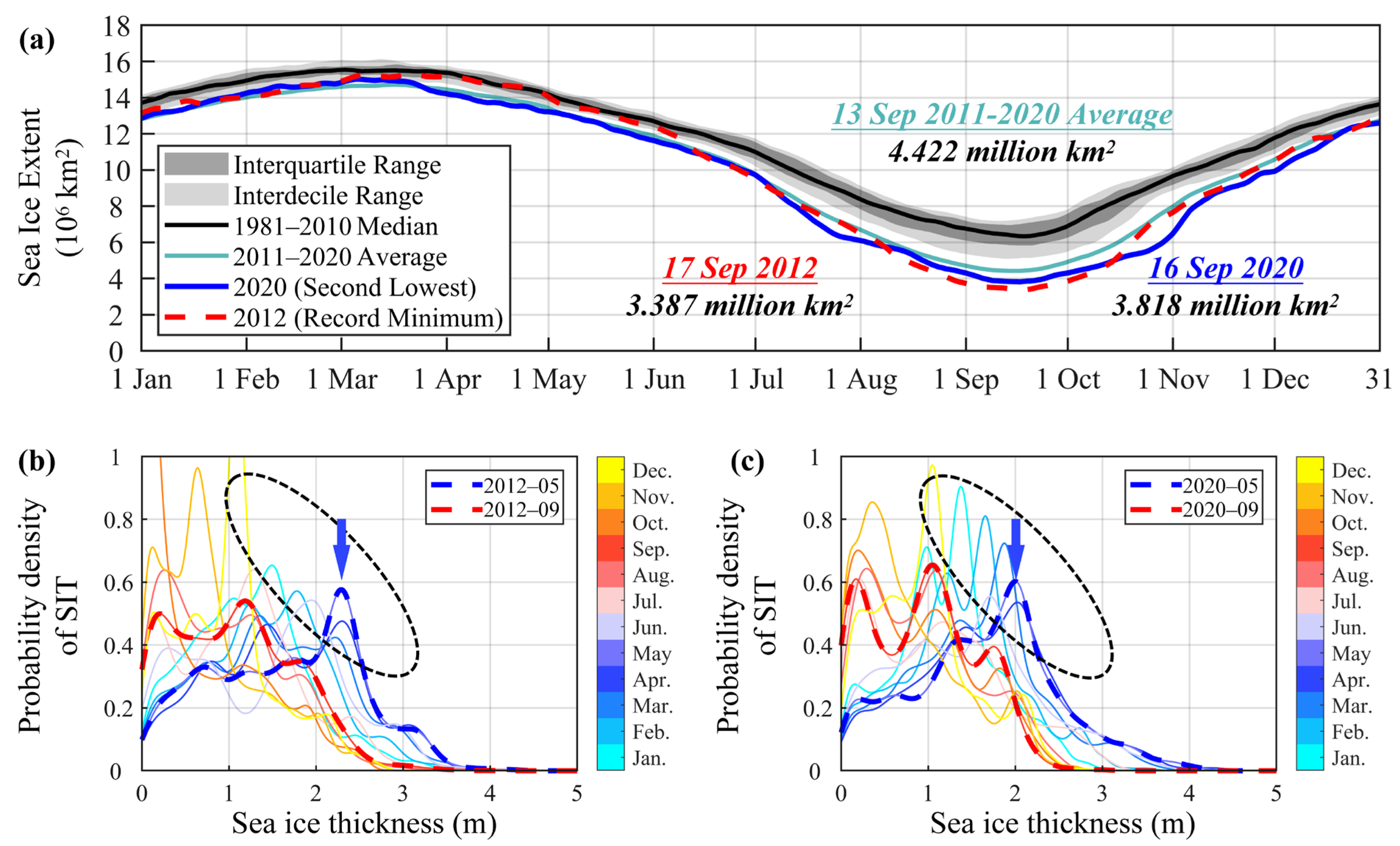
We define extreme melting years as those with annual minimum September sea ice extent (SIE), the climatological seasonal trough explicitly presented in Figure 15a. SIE here is calculated from NSIDC SIC data identical to ICE-3D input. As auxiliary background rather than a core variable, it is adopted to compare seasonal discrepancies between the two extreme ice-melting years (2012: record SIE minimum; 2020: second-lowest SIE) and climatological periods, and to verify the adaptability of our ICE-3D SIT product under extreme summer melting [55].

Figure 15. (a) Annual seasonal cycle of Arctic SIE from NSIDC SIC. Monthly SIT probability density distributions from ICE-3D for (b) 2012 and (c) 2020; the color bar denotes calendar months.

ICE-3D reconstructs daily Arctic SIT from 1979 to 2023 (45 years) and yields complete summer SIT records, enabling analysis of seasonal SIT evolution throughout the melting season. As shown in Figure 15a, Arctic SIE peaks in late winter and declines continuously until reaching the annual minimum in September. The minimum SIE during 2011–2020 is more than 30% smaller than the minimum SIE during 1981–2010. In 2012, the SIE decreased from a maximum of 15.294 to a minimum of 3.387, with a nearly 78% reduction. In 2020, it decreased from a maximum of 15.018 to a minimum of 3.818, with a change rate of nearly 75%. These observed shifts in Arctic sea ice seasonal patterns are consistent with long-term trends reported in previous research, where such interannual variability has been attributed to climate change [56].

To reveal the thickness-driven mechanism behind these SIE differences, we compare monthly SIT probability density distributions of 2012 and 2020 from ICE-3D (Figure 15b,c). Overall, Arctic sea ice was thinner in 2020 than 2012: thick ice (>2 m) sharply declined, while thin ice (<1.5 m) expanded markedly. This homogenization transition indicates that multi-year thick ice is progressively replaced by young seasonal thin ice, and that the contemporary Arctic thermal regime can no longer sustain thick ice formation [57,58], consistent with prior studies [52,59]. The record-low SIE in 2012 originated from insufficient medium-to-thick ice reserves accumulated in winter; limited thick ice cannot buffer summer heat input, leading to rapid depletion of young thin ice [56]. Though seasonal ice decay processes remain complex [60], ICE-3D provides refined spatial SIT structures to interpret such extreme seasonal variations.

5.2. Inter-Annual Variability

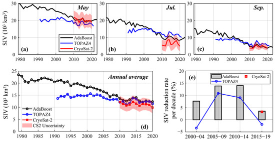
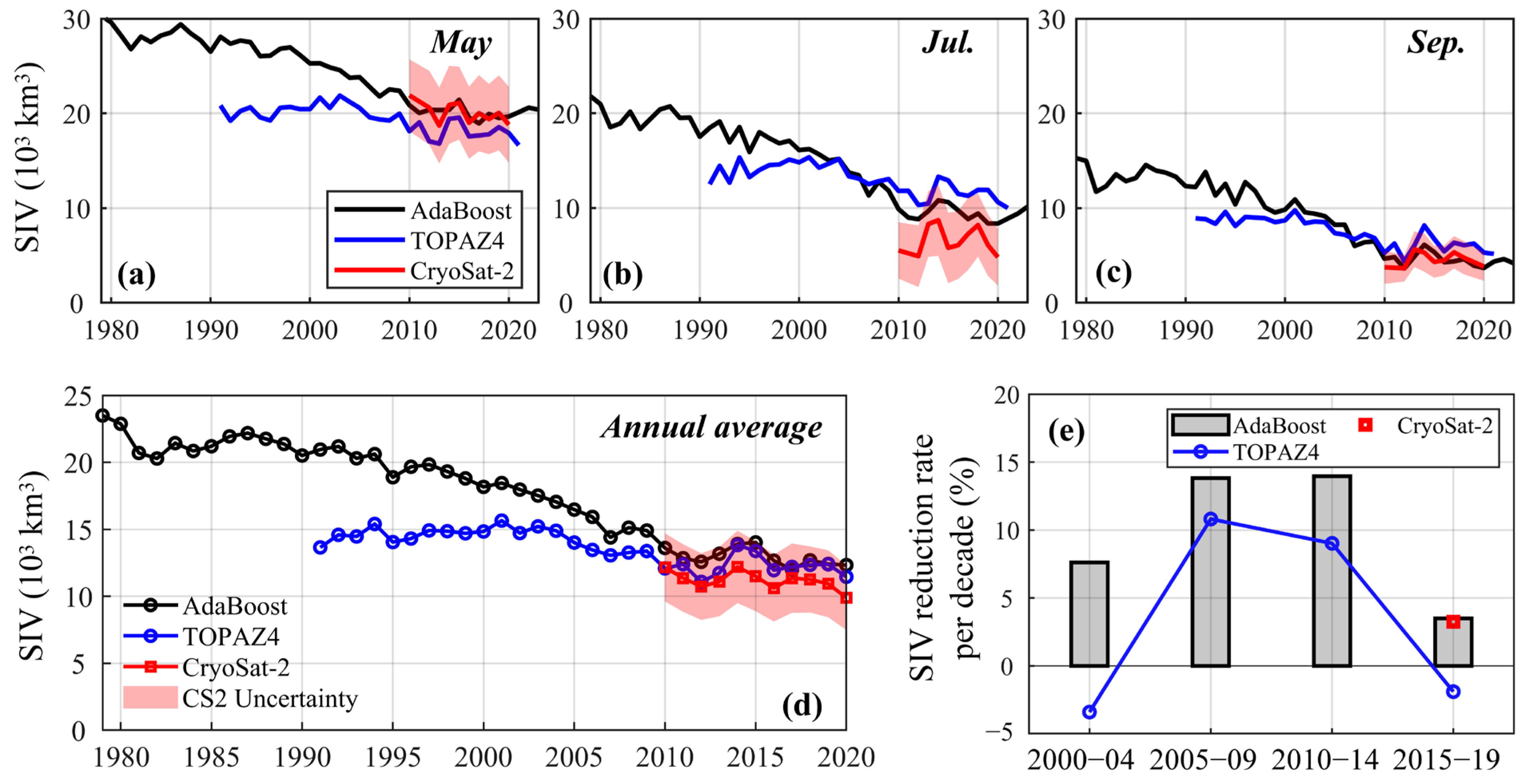
Pan-Arctic SIV is spatially integrated from gridded ICE-3D SIT outputs. Figure 16 shows monthly and annual SIV trends, validated against TOPAZ4 reanalysis and CryoSat-2 satellite observations. ICE-3D SIV trends closely agree with CryoSat-2, particularly in May and September. By contrast, TOPAZ4 yields conservative estimates: it mitigates winter SIV overestimation, yet it underestimates summer sea ice ablation rates. Validated against CryoSat-2 satellite data and BGEP in situ measurements (Figure 12), ICE-3D exhibits superior reliability for summertime SIV reconstruction.

Figure 16. Trend analysis of the pan-Arctic annual average SIV from 1979 to 2023. The 45-year trend of SIV in (a) May, (b) July, and (c) September. (d) The trend of the annual average SIV. (e) The 5-year sliding SIV decay rate from 2000 to 2019.

From 1979 to 2020, ICE-3D-derived SIV declined from 23.49 to 12.92 (×10³ km³), corresponding to a 44% total ice loss across 45 years. This long-term trend carries uncertainties originating from the PIOMAS training dataset. From 1991 to 2020, SIV decreased by 38% in ICE-3D versus merely 18% in TOPAZ4. During 2010–2020, CryoSat-2 recorded a 19% SIV reduction, while the decay rates were 13% and 7% for ICE-3D and TOPAZ4, respectively. Distinct discrepancies exist among datasets, and ICE-3D aligns best with CryoSat-2, our independent benchmark for grid-scale SIT validation. Five-year sliding decay rates further confirm persistent positive SIV loss in ICE-3D, consistent with CryoSat-2, whereas TOPAZ4 occasionally produces unrealistic positive SIV anomalies [57].

ICE-3D reveals a pronounced long-term SIV decline, alongside a moderated melting rate captured jointly with CryoSat-2. This slowdown does not indicate halted melting or climatic recovery; the sustained downward trajectory implies that Arctic sea ice loss is largely irreversible under current climate conditions. Since 2007, Arctic sea ice has shifted into a new regime dominated by thin, homogeneous ice. Depleted thick perennial ice substantially narrows the seasonal variability range of total SIV [61].

5.3. Limitations and Quantitative Uncertainty Assessment

We found that there was little difference in the performance of the error metrics among AdaBoost, LightGBM, and Random Forest. However, the Wilcoxon signed-rank test confirmed that AdaBoost had a statistically significant advantage (Figure S3). Tree-based ensemble algorithms were chosen as backbones to verify STMFW efficacy, striking a balance between computational efficiency, noise resilience and interpretability while avoiding excessive computational overhead. Of course, deep learning models have shown promise in sea ice studies, but they require massive amounts of manually annotated datasets, which may introduce additional uncertainty.

Existing machine learning SIT reconstruction methods generally adopt static single-scale frameworks with fixed temporal windows and one-off offline training, and are mostly limited to wintertime or regional applications. Such designs cannot separate short-term abrupt ice fluctuations from long-term climate trends, nor adapt to interannual shifts in the Arctic sea ice system. ICE-3D leverages the STMFW for multiscale spatiotemporal feature fusion paired with online incremental learning, which continuously updates parameters using time-evolving samples to capture full-year ice variations and notably improves summer SIT reconstruction under data scarcity. We validated this improvement via ablation tests (Figure S4): the online learning scheme yields lower MAE and alleviates temporal generalization drift that causes substantial SIT overestimation in marginal ice zones for static offline models.

PIOMAS and ERA5 assimilate mature satellite observations, and the inter-product bias between these paired predictors is mainly localized in marginal ice zones with limited basin-scale systematic deviation (Figures S5 and S6). However, mismatches in localized areas remain a source of residual uncertainty in the reconstruction results. Long-term SIT trends inherit a cumulative relative uncertainty of ±7% from PIOMAS. This total uncertainty originates from intrinsic biases within the PIOMAS reanalysis (atmospheric forcing errors, sea ice parameterization deviations) plus propagated fitting uncertainty introduced during model training, which bounds the overall range of our multi-decadal sea ice loss estimates. The fixed 25 km NSIDC grid cannot resolve fine-scale ice features within fjords and archipelagos, smoothing coastal gradients and underestimating localized thin ice variability. It should be noted that pan-Arctic summer SIT validation is hampered by scarce reliable observation records. Our summer assessment mainly depends on biweekly CryoSat-2 altimetry and sparse BGEP mooring data. Summer CryoSat-2 retrievals are biased by melt pond coverage and surface melting, with a typical absolute uncertainty of 0.45–0.75 m for thin ice (<1.5 m). BGEP moorings are limited to marginal seas and lack basin-wide coverage. Therefore, the MAE of ICE-3D SIT relative to BGEP is ~0.5 m, with summer uncertainty slightly higher than winter. This is also the challenge of quantifying uncertainty given SIT observation limitations. Therefore, summer comparisons between ICE-3D and reanalysis require cautious interpretation, and comprehensive validation awaits denser summertime in situ and satellite observations. Moreover, the current data-driven model lacks embedded thermodynamic and dynamic constraints, occasionally generating unphysical SIT extremes in data-sparse marginal seas, which is also a major source of uncertainty in ICE-3D.

6. Conclusions

This study proposes a spatiotemporal multiscale inference framework based on ML, referred to as ICE-3D, to integrate multi-satellite observations and atmospheric conditions for estimating Arctic daily SIT. We designed an innovative training strategy (STMFW) to integrate historical, seasonal, and near-term evolution information and key geographic features. We have verified that ICE-3D has great application advantages, especially in providing relatively objective and complete analysis results when Arctic SIT observations are missing. Within the coverage of available summer observational constraints, ICE-3D exhibits favorable summer SIT reconstruction performance relative to TOPAZ4 and PIOMAS. We note that this comparison is limited by sparse summer validation data.

Our study draws the following conclusions: (1) AdaBoost in the ICE-3D framework has the best performance. The STMFW training strategy enhances the performance of all models, with a daily inference time of no more than 30 s. (2) We effectively reconstruct daily pan-Arctic SIT from 1979 to 2023 with a spatial resolution of 25 km. (3) ICE-3D provides more accurate summer SIT and more reasonable estimates of the long-term trend of SIV. The ICE-3D results are highly consistent with SIT observations, particularly in capturing high-frequency regional evolution and seasonal SIV changes. (4) The results from ICE-3D suggest that Arctic sea ice has undergone a regime shift, becoming thinner and more uniform. About 38% of Arctic sea ice disappeared from 1991 to 2020. Over the past decade, the rate of Arctic sea ice melt has stabilized, which may indicate that Arctic sea ice reserves may be critically deficient and that losses are potentially irreversible.

In the future, we plan to further refine the ICE-3D framework along two main directions: First, we will downscale the ICE-3D framework to achieve higher spatial resolution by incorporating fine-resolution satellite remote sensing data, and will further optimize the STMFW module to capture coastal and fjord-scale localized sea ice variations for regional Arctic research. Second, physical regularizers derived from coupled ice–ocean numerical models will be embedded into the data-driven workflow to suppress unphysical SIT predictions, reduce reconstruction bias in observation-sparse marginal seas, and strengthen the physical interpretability of the machine learning framework. These improvements will support the generation of high-spatiotemporal-resolution, physically consistent long-term Arctic SIT climate datasets.

References

- Bacon, S. Arctic Sea Ice, Ocean, and Climate Evolution. Science 2023, 381, 946–947. [Google Scholar] [CrossRef] [Scilit] [PubMed]
- Rantanen, M.; Karpechko, A.Y.; Lipponen, A.; Nordling, K.; Hyvärinen, O.; Ruosteenoja, K.; Vihma, T.; Laaksonen, A. The Arctic Has Warmed Nearly Four Times Faster than the Globe since 1979. Commun. Earth Environ. 2022, 3, 168. [Google Scholar] [CrossRef] [Scilit]
- Barkhordarian, A.; Nielsen, D.M.; Olonscheck, D.; Baehr, J. Arctic Marine Heatwaves Forced by Greenhouse Gases and Triggered by Abrupt Sea-Ice Melt. Commun. Earth Environ. 2024, 5, 57. [Google Scholar] [CrossRef] [Scilit]
- Dong, J.; Shi, X.; Gong, X.; Astakhov, A.S.; Hu, L.; Liu, X.; Yang, G.; Wang, Y.; Vasilenko, Y.; Qiao, S.; et al. Enhanced Arctic Sea Ice Melting Controlled by Larger Heat Discharge of Mid-Holocene Rivers. Nat. Commun. 2022, 13, 5368. [Google Scholar] [CrossRef] [Scilit] [PubMed]
- Jahn, A.; Holland, M.M.; Kay, J.E. Projections of an Ice-Free Arctic Ocean. Nat. Rev. Earth Environ. 2024, 5, 164–176. [Google Scholar] [CrossRef] [Scilit]
- Heuzé, C.; Jahn, A. The First Ice-Free Day in the Arctic Ocean Could Occur before 2030. Nat. Commun. 2024, 15, 10101. [Google Scholar] [CrossRef] [Scilit] [PubMed]
- Zhao, P.; Li, Y.; Zhang, Y. Ships Are Projected to Navigate Whole Year-Round along the North Sea Route by 2100. Commun. Earth Environ. 2024, 5, 407. [Google Scholar] [CrossRef] [Scilit]
- Zheng, Q.; Shao, Q.; Li, H.; Han, G.; Li, W.; Cao, L.; Zhou, G.; Wu, H.; Luo, Q.; Liu, H.; et al. A Data-Driven Model for Seasonal Regional Arctic Ice-Ocean Coupling Prediction: Modeling and Preliminary Evaluation. J. Phys. Conf. Ser. 2026, 3178, 012040. [Google Scholar] [CrossRef] [Scilit]
- Zheng, Q.; Li, W.; Shao, Q.; Han, G.; Wang, X. A Mid- and Long-Term Arctic Sea Ice Concentration Prediction Model Based on Deep Learning Technology. Remote Sens. 2022, 14, 2889. [Google Scholar] [CrossRef] [Scilit]
- Zheng, Q.; Wang, R.; Han, G.; Li, W.; Wang, X.; Shao, Q.; Wu, X.; Cao, L.; Zhou, G.; Hu, S. A Spatiotemporal Multiscale Deep Learning Model for Subseasonal Prediction of Arctic Sea Ice. IEEE Trans. Geosci. Remote Sens. 2024, 62, 1–22. [Google Scholar] [CrossRef] [Scilit]
- Lyu, G.; Koehl, A.; Serra, N.; Stammer, D.; Xie, J. Arctic Ocean–Sea Ice Reanalysis for the Period 2007–2016 Using the Adjoint Method. Q. J. R. Meteorol. Soc. 2021, 147, 1908–1929. [Google Scholar] [CrossRef] [Scilit]
- Cartwright, J.; Banks, C.J.; Srokosz, M. Sea Ice Detection Using GNSS-R Data From TechDemoSat-1. J. Geophys. Res. Oceans 2019, 124, 5801–5810. [Google Scholar] [CrossRef] [Scilit]
- Cooke, C.L.V.; Scott, K.A. Estimating Sea Ice Concentration From SAR: Training Convolutional Neural Networks with Passive Microwave Data. IEEE Trans. Geosci. Remote Sens. 2019, 57, 4735–4747. [Google Scholar] [CrossRef] [Scilit]
- Huang, Y.; Ren, Y.; Li, X. Deep Learning Techniques for Enhanced Sea-Ice Types Classification in the Beaufort Sea via SAR Imagery. Remote Sens. Environ. 2024, 308, 114204. [Google Scholar] [CrossRef] [Scilit]
- Park, J.-W.; Korosov, A.A.; Babiker, M.; Won, J.-S.; Hansen, M.W.; Kim, H.-C. Classification of Sea Ice Types in Sentinel-1 Synthetic Aperture Radar Images. Cryosphere 2020, 14, 2629–2645. [Google Scholar] [CrossRef] [Scilit]
- Laxon, S.W.; Giles, K.A.; Ridout, A.L.; Wingham, D.J.; Willatt, R.; Cullen, R.; Kwok, R.; Schweiger, A.; Zhang, J.; Haas, C.; et al. CryoSat-2 Estimates of Arctic Sea Ice Thickness and Volume. Geophys. Res. Lett. 2013, 40, 732–737. [Google Scholar] [CrossRef] [Scilit]
- Paţilea, C.; Heygster, G.; Huntemann, M.; Spreen, G. Combined SMAP–SMOS Thin Sea Ice Thickness Retrieval. Cryosphere 2019, 13, 675–691. [Google Scholar] [CrossRef] [Scilit]
- Ricker, R.; Hendricks, S.; Kaleschke, L.; Tian-Kunze, X.; King, J.; Haas, C. A Weekly Arctic Sea-Ice Thickness Data Record from Merged CryoSat-2 and SMOS Satellite Data. Cryosphere 2017, 11, 1607–1623. [Google Scholar] [CrossRef] [Scilit]
- Fiedler, E.K.; Martin, M.J.; Blockley, E.; Mignac, D.; Fournier, N.; Ridout, A.; Shepherd, A.; Tilling, R. Assimilation of Sea Ice Thickness Derived from CryoSat-2 along-Track Freeboard Measurements into the Met Office’s Forecast Ocean Assimilation Model (FOAM). Cryosphere 2022, 16, 61–85. [Google Scholar] [CrossRef] [Scilit]
- Min, C.; Yang, Q.; Luo, H.; Chen, D.; Krumpen, T.; Mamnun, N.; Liu, X.; Nerger, L. Improving Arctic Sea-Ice Thickness Estimates with the Assimilation of CryoSat-2 Summer Observations. Ocean-Land-Atmos. Res. 2023, 2, 0025. [Google Scholar] [CrossRef] [Scilit]
- Zhang, Y.-F.; Bushuk, M.; Winton, M.; Hurlin, B.; Gregory, W.; Landy, J.; Jia, L. Improvements in September Arctic Sea Ice Predictions Via Assimilation of Summer CryoSat-2 Sea Ice Thickness Observations. Geophys. Res. Lett. 2023, 50, e2023GL105672. [Google Scholar] [CrossRef] [Scilit]
- Landy, J.C.; Dawson, G.J.; Tsamados, M.; Bushuk, M.; Stroeve, J.C.; Howell, S.E.L.; Krumpen, T.; Babb, D.G.; Komarov, A.S.; Heorton, H.D.B.S.; et al. A Year-Round Satellite Sea-Ice Thickness Record from CryoSat-2. Nature 2022, 609, 517–522. [Google Scholar] [CrossRef] [Scilit] [PubMed]
- Dawson, G.; Landy, J.; Tsamados, M.; Komarov, A.S.; Howell, S.; Heorton, H.; Krumpen, T. A 10-Year Record of Arctic Summer Sea Ice Freeboard from CryoSat-2. Remote Sens. Environ. 2022, 268, 112744. [Google Scholar] [CrossRef] [Scilit]
- Yan, Q.; Huang, W. Sea Ice Thickness Estimation From TechDemoSat-1 and Soil Moisture Ocean Salinity Data Using Machine Learning Methods. In Proceedings of the Global Oceans 2020: Singapore–U.S. Gulf Coast; Biloxi, MS, USA, 5–30 October 2020, pp. 1–5.
- Shamshiri, R.; Eide, E.; Høyland, K.V. Spatio-Temporal Distribution of Sea-Ice Thickness Using a Machine Learning Approach with Google Earth Engine and Sentinel-1 GRD Data. Remote Sens. Environ. 2022, 270, 112851. [Google Scholar] [CrossRef] [Scilit]
- Li, H.; Yan, Q.; Huang, W. Retrieval of Sea Ice Thickness from FY-3E Data Using Random Forest Method. Adv. Space Res. 2024, 74, 130–144. [Google Scholar] [CrossRef] [Scilit]
- Belter, H.J.; Krumpen, T.; von Albedyll, L.; Alekseeva, T.A.; Birnbaum, G.; Frolov, S.V.; Hendricks, S.; Herber, A.; Polyakov, I.; Raphael, I.; et al. Interannual Variability in Transpolar Drift Summer Sea Ice Thickness and Potential Impact of Atlantification. Cryosphere 2021, 15, 2575–2591. [Google Scholar] [CrossRef] [Scilit]
- Bushuk, M.; Winton, M.; Bonan, D.B.; Blanchard-Wrigglesworth, E.; Delworth, T.L. A Mechanism for the Arctic Sea Ice Spring Predictability Barrier. Geophys. Res. Lett. 2020, 47, e2020GL088335. [Google Scholar] [CrossRef] [Scilit]
- Kaleschke, L.; Tian-Kunze, X.; Hendricks, S.; Ricker, R. SMOS-Derived Antarctic Thin Sea Ice Thickness: Data Description and Validation in the Weddell Sea. Earth Syst. Sci. Data 2024, 16, 3149–3170. [Google Scholar] [CrossRef] [Scilit]
- Trivedi, S.; Sievers, I.; Athanase, M.; Sánchez-Benítez, A.; Semmler, T. Evaluating Arctic Sea Ice and Snow Thickness Simulations: Methodological Insights from MOSAiC and CMIP6 Data. Front. Earth Sci. 2026, 14, 1744420. [Google Scholar] [CrossRef] [Scilit]
- Wu, H.; Wang, Y.; Zhang, R.; Yan, H.; Hong, M. Bias Correction of Arctic Sea Ice Thickness Products Based on Factor Selection and Machine Learning Methods. Appl. Ocean Res. 2024, 149, 104069. [Google Scholar] [CrossRef] [Scilit]
- Ma, Z.; Nie, Y.; Luo, H.; Liu, J.; Yang, Q. An Improved Antarctic Sea Ice Thickness Dataset Derived from CryoSat-2 Using LightGBM. Adv. Atmos. Sci. 2026, 43, 2005–2018. [Google Scholar] [CrossRef] [Scilit]
- René-Bazin, E.; Tsamados, M.; Raziuddin, S.S.B.A.; Perez Ferrer, J.; Suciu, T.; Nab, C.; Ghag, C.; Heorton, H.; Willatt, R.; Landy, J.; et al. Bayesian Inversion of Satellite Altimetry for Arctic Sea Ice and Snow Thickness. Cryosphere 2026, 20, 3913–3932. [Google Scholar] [CrossRef] [Scilit]
- Kimura, N.; Hasumi, H. Estimating Arctic Sea Ice Thickness from Satellite-Based Ice History. Cryosphere 2026, 20, 2331–2349. [Google Scholar] [CrossRef] [Scilit]
- Xie, Y.; Duan, A.; Zhang, C.; He, C.; Mao, Q.; Liu, B. Reversed Link between Central Pacific ENSO and Greenland–Barents Sea Ice. npj Clim. Atmos. Sci. 2025, 8, 28. [Google Scholar] [CrossRef] [Scilit]
- Feng, J.; Zhang, Y.; Cheng, Q.; Tsou, J.Y. Pan-Arctic Melt Pond Fraction Trend, Variability, and Contribution to Sea Ice Changes. Glob. Planet. Change 2022, 217, 103932. [Google Scholar] [CrossRef] [Scilit]
- Martínez-Moreno, J.; Lique, C.; Talandier, C. Sea Ice Heterogeneity as a Result of Ocean Eddy Activity During the Ice Growth Season. Geophys. Res. Lett. 2025, 52, e2024GL113645. [Google Scholar] [CrossRef] [Scilit]
- Wang, X.; Li, S.; Zhao, Y.; Wang, Y.; Yang, Z. Comparison of Arctic and Antarctic Sea Ice Spatial–Temporal Changes during 1979–2018. J. Hydrol. 2024, 632, 130966. [Google Scholar] [CrossRef] [Scilit]
- Zhang, J.; Rothrock, D.A. Modeling Global Sea Ice with a Thickness and Enthalpy Distribution Model in Generalized Curvilinear Coordinates. Mon. Weather Rev. 2003, 131, 845–861. [Google Scholar] [CrossRef]
- Hersbach, H.; Bell, B.; Berrisford, P.; Hirahara, S.; Horányi, A.; Muñoz-Sabater, J.; Nicolas, J.; Peubey, C.; Radu, R.; Schepers, D.; et al. The ERA5 Global Reanalysis. Q. J. R. Meteorol. Soc. 2020, 146, 1999–2049. [Google Scholar] [CrossRef] [Scilit]
- Huang, B.; Liu, C.; Banzon, V.; Freeman, E.; Graham, G.; Hankins, B.; Smith, T.; Zhang, H.-M. Improvements of the Daily Optimum Interpolation Sea Surface Temperature (DOISST) Version 2.1. J. Clim. 2021, 34, 2923–2939. [Google Scholar] [CrossRef] [Scilit]
- Kaleschke, L.; Tian-Kunze, X.; Maaß, N.; Mäkynen, M.; Drusch, M. Sea Ice Thickness Retrieval from SMOS Brightness Temperatures during the Arctic Freeze-up Period. Geophys. Res. Lett. 2012, 39, L05501. [Google Scholar] [CrossRef] [Scilit]
- Melling, H.; Johnston, P.H.; Riedel, D.A. Measurements of the Underside Topography of Sea Ice by Moored Subsea Sonar. J. Atmos. Ocean. Technol. 1995, 12, 589–602. [Google Scholar] [CrossRef]
- Nguyen, A.T.; Menemenlis, D.; Kwok, R. Arctic Ice-Ocean Simulation with Optimized Model Parameters: Approach and Assessment. J. Geophys. Res. Oceans 2011, 116, C04025. [Google Scholar] [CrossRef] [Scilit]
- Sakov, P.; Counillon, F.; Bertino, L.; Lisæter, K.A.; Oke, P.R.; Korablev, A. TOPAZ4: An Ocean-Sea Ice Data Assimilation System for the North Atlantic and Arctic. Ocean Sci. 2012, 8, 633–656. [Google Scholar] [CrossRef] [Scilit]
- Kotsiantis, S.B. Decision Trees: A Recent Overview. Artif. Intell. Rev. 2013, 39, 261–283. [Google Scholar] [CrossRef] [Scilit]
- Belgiu, M.; Drăguţ, L. Random Forest in Remote Sensing: A Review of Applications and Future Directions. ISPRS J. Photogramm. Remote Sens. 2016, 114, 24–31. [Google Scholar] [CrossRef] [Scilit]
- Chen, T.; Guestrin, C. XGBoost: A Scalable Tree Boosting System. In Proceedings of the 22nd ACM SIGKDD International Conference on Knowledge Discovery and Data Mining, San Francisco, CA, USA, 13–17 August 2016; ACM: New York, NY, USA, 2016; pp. 785–794. [Google Scholar]
- Ke, G.; Meng, Q.; Finley, T.; Wang, T.; Chen, W.; Ma, W.; Ye, Q.; Liu, T.-Y. LightGBM: A Highly Efficient Gradient Boosting Decision Tree. In Proceedings of the Neural Information Processing Systems, Long Beach, CA, USA, 4–9 December 2017. [Google Scholar]
- Freund, Y.; Schapire, R.E. A Decision-Theoretic Generalization of On-Line Learning and an Application to Boosting. J. Comput. Syst. Sci. 1997, 55, 119–139. [Google Scholar] [CrossRef] [Scilit]
- Pedregosa, F.; Varoquaux, G.; Gramfort, A.; Michel, V.; Thirion, B.; Grisel, O.; Blondel, M.; Prettenhofer, P.; Weiss, R.; Dubourg, V.; et al. Scikit-Learn: Machine Learning in Python. J. Mach. Learn. Res. 2011, 12, 2825–2830. [Google Scholar]
- Sumata, H.; de Steur, L.; Divine, D.V.; Granskog, M.A.; Gerland, S. Regime Shift in Arctic Ocean Sea Ice Thickness. Nature 2023, 615, 443–449. [Google Scholar] [CrossRef] [Scilit] [PubMed]
- Schweiger, A.; Lindsay, R.; Zhang, J.; Steele, M.; Stern, H.; Kwok, R. Uncertainty in Modeled Arctic Sea Ice Volume. J. Geophys. Res. Oceans 2011, 116, C00D06. [Google Scholar] [CrossRef] [Scilit]
- Farrell, S.L.; Duncan, K.; Buckley, E.M.; Richter-Menge, J.; Li, R. Mapping Sea Ice Surface Topography in High Fidelity with ICESat-2. Geophys. Res. Lett. 2020, 47, e2020GL090708. [Google Scholar] [CrossRef] [Scilit]
- Meier, W.N.; Hovelsrud, G.K.; van Oort, B.E.H.; Key, J.R.; Kovacs, K.M.; Michel, C.; Haas, C.; Granskog, M.A.; Gerland, S.; Perovich, D.K.; et al. Arctic Sea Ice in Transformation: A Review of Recent Observed Changes and Impacts on Biology and Human Activity. Rev. Geophys. 2014, 52, 185–217. [Google Scholar] [CrossRef] [Scilit]
- Finocchio, P.M.; Stern, D.P.; Doyle, J.D.; Perovich, D.K. Observed Drivers of Rapid Sea-Ice Melt Events in the Arctic During Summer. Geophys. Res. Lett. 2026, 53, e2026GL121848. [Google Scholar] [CrossRef] [Scilit]
- Bocquet, M.; Fleury, S.; Rémy, F.; Piras, F. Arctic and Antarctic Sea Ice Thickness and Volume Changes From Observations Between 1994 and 2023. J. Geophys. Res. Oceans 2024, 129, e2023JC020848. [Google Scholar] [CrossRef] [Scilit]
- Zhang, Y.; Chen, C.; Beardsley, R.C.; Gao, G.; Qi, J.; Lin, H. Seasonal and Interannual Variability of the Arctic Sea Ice: A Comparison between AO-FVCOM and Observations. J. Geophys. Res. Oceans 2016, 121, 8320–8350. [Google Scholar] [CrossRef] [Scilit]
- Bushuk, M.; Giannakis, D. The Seasonality and Interannual Variability of Arctic Sea Ice Reemergence. J. Clim. 2017, 30, 4657–4676. [Google Scholar] [CrossRef] [Scilit]
- Richter-Menge, J.A.; Farrell, S.L. Arctic Sea Ice Conditions in Spring 2009–2013 Prior to Melt. Geophys. Res. Lett. 2013, 40, 5888–5893. [Google Scholar] [CrossRef] [Scilit]
- Soriot, C.; Vancoppenolle, M.; Prigent, C.; Jimenez, C.; Frappart, F. Winter Arctic Sea Ice Volume Decline: Uncertainties Reduced Using Passive Microwave-Based Sea Ice Thickness. Sci. Rep. 2024, 14, 21000. [Google Scholar] [CrossRef] [Scilit] [PubMed]
Disclaimer/Publisher’s Note: The statements, opinions and data contained in all publications are solely those of the individual author(s) and contributor(s) and not of MDPI and/or the editor(s). MDPI and/or the editor(s) disclaim responsibility for any injury to people or property resulting from any ideas, methods, instructions or products referred to in the content. |
© 2026 by the authors. Licensee MDPI, Basel, Switzerland. This article is an open access article distributed under the terms and conditions of the Creative Commons Attribution (CC BY) license.