Physically Constrained Quadratic Programming for Spectral Unmixing of Nighttime Lighting: A Case Study with Data Generation Procedure

Highlights

What are the main findings?

• A physically constrained quadratic programming framework for spectral unmixing extends the conventional fully constrained least squares formulation by combining abundance non-negativity, a relaxed abundance-sum constraint, and a residual-positivity constraint derived from the physics of illumination mixtures.
• Using a physically motivated data generation framework and measured outdoor illumination spectra, the proposed formulation improves the robustness of abundance estimation in the presence of surface reflections and unknown spectral contributions while maintaining accuracy for conventional mixtures.

What are the implications of the main findings?

• Incorporating physically interpretable inequality constraints into convex spectral unmixing improves solution reliability when the observed spectrum contains contributions that cannot be represented by the available endmember library.
• The proposed data generation framework and constrained unmixing formulation can be readily integrated into spectral unmixing applications where a spectral library is available but the observed spectra may include unknown spectral components.

Abstract

Spectral unmixing of outdoor nighttime lighting mixtures is a linear but challenging problem due to spectral variability and contributions from unknown light sources. This paper presents a quadratic programming algorithm for constrained linear unmixing abundance estimation that extends the conventional fully constrained least squares approach through a physically motivated set of three linear constraints: estimated abundances must be non-negative, their sum must not be greater than unity, and the spectral signature reconstructed from estimated abundances must not exceed the measured signal in any spectral band. Unlike alternative optimization or neural network approaches, the proposed formulation requires no hyperparameter tuning or stochastic training, and yields a unique globally optimal solution whenever the endmember spectra are linearly independent, as verified for the case study considered here. The accuracy of the algorithm is evaluated using a physically motivated dataset generation framework grounded in the Generalized Linear Mixing Model, which is capable of modeling wavelength-dependent surface reflections and variable fractions of unknown light sources. Experiments conducted on a database of measured illumination sources demonstrate that the proposed formulation outperforms the classical fully constrained least squares baseline. Specifically, it reduces the abundance RMSE from 0.1539 to 0.1484 and improves the endmember detection F1 score from 0.795 to 0.803, with differences confirmed to be statistically significant. Furthermore, the model remains robust to surface reflections present in up to 80% of the evaluated mixtures. It maintains reliable abundance estimates for unknown spectral contributions up to approximately 15%, with accuracy gradually decreasing beyond this level. Finally, both the optimization method and the dataset generation framework are completely independent of the underlying channel configuration, making them readily adaptable to arbitrary choices of spectral channels and application domains beyond public lighting analysis.

1. Introduction

Spectral unmixing is a fundamental problem in hyperspectral and multispectral signal analysis, with applications spanning remote sensing, environmental monitoring, material identification, biomedicine, and illumination analysis [1,2,3,4,5]. Its objective is to decompose an observed spectrum into a set of constituent spectral signatures, commonly referred to as endmembers, and estimate their fractional contributions to the mixture. The problem is inherently ill-posed, particularly when the number of available spectral channels is limited, reference spectra are highly correlated, and the observed signal may contain contributions from unknown light sources.

The Linear Mixing Model (LMM) [6] is the most widely used framework for spectral unmixing. This study focuses specifically on the mixtures of human-made illumination sources in outdoor environments, where the linear mixing assumption is justified. The observed signal is formed as a superposition of the spectral radiant power from multiple independent light sources, with no interaction between them prior to detection. Light sources are mutually incoherent, with no interference effects, and the sensor response can be considered linear. The effects that would introduce nonlinear mixing, such as multiple scattering, nonlinear absorption, or coherent interference, are negligible under typical night-time outdoor illumination conditions.

This focus on human-made illumination sources directly addresses a concrete application need in urban environmental monitoring. Public lighting is currently transitioning from legacy discharge lamps, such as high-pressure sodium and metal-halide, to modern LED technology. Monitoring this shift requires unmixing the resulting light signal into its constituent lamp types. Furthermore, the spectral composition of artificial light at night determines the impact of light pollution and night sky glow. Unmixing the illumination spectrum is therefore a necessary step toward attributing light pollution to specific lamp technologies. This task fundamentally differs from classical remote sensing, where endmembers typically represent natural materials distinguished by their reflectance. In contrast, our framework models active light sources whose emission characteristics interact directly with the reflecting urban surfaces.

We adopt the quadratic programming (QP) formulation for spectral unmixing, as it provides a natural framework for minimizing a convex quadratic objective under linear constraints. This enables direct incorporation of physically meaningful constraints, without the need for hyperparameter tuning or stochastic training. Alternative approaches include sparse unmixing via variable splitting and augmented Lagrangian (SUnSAL) [7,8], probabilistic methods [9,10], and various neural network architectures such as autoencoders [11,12], multi-domain convolutional networks [13], and attention-based architectures [14,15]. These methods are efficient for large endmember libraries and can capture complex spectral variations. However, sparse unmixing methods like SUnSAL may require careful tuning of the regularization parameter and can be sensitive to the coherence of the spectral library. Probabilistic methods may require suitable prior distributions and can be computationally demanding, whereas neural network architectures require substantial amounts of training data and are often more challenging to interpret [16].

Beyond these optimization and learning-based approaches, earlier research has targeted several specific aspects of this problem. For example, operating with incomplete or partially known endmember libraries has a long background in the literature on target detection. There, orthogonal subspace projection [17] suppresses interference from unmodeled background signatures without requiring them in the library, while more recent nonnegative matrix factorization formulations extend this idea to incomplete and noisy hyperspectral data [18]. Other methods use residual or additive terms to absorb outliers, background contributions, or model mismatch. Examples include mismodelling effect terms constrained to be spectrally smooth and spatially sparse [19], or robust formulations that treat the residual as a sparse outlier component within a collaborative sparse regression framework [20]. Similarly, the abundance sum-to-one constraint has been relaxed before; partially constrained least-squares formulations for subpixel target detection discard the sum constraint entirely to accommodate background or unmodeled materials absent from the target library [21]. Unlike these approaches, our formulation combines a relaxed sum constraint with a residual-positivity constraint motivated specifically by the physical structure of active source illumination mixtures. Instead of relying on traditional interference suppression for detecting targets, background modeling, or regularization that promotes sparsity, we introduce a constraint ensuring that the reconstructed energy does not fall below the measured energy. This combination has not been previously proposed for spectral unmixing.

Several models have been proposed in the literature to address spectral variability, including the Extended Linear Mixing Model (ELMM) [22], the Augmented Linear Mixing Model (ALMM) [23], the Scaled and Perturbed Linear Mixing Model (SPLMM) [24,25], and the Generalized Linear Mixing Model (GLMM) [26], as well as broader formulations and taxonomies [27]. The GLMM can be viewed as a straightforward, band-dependent extension of the standard LMM introduced to account for spectral variability while preserving the linear structure of the model. In contrast, ELMM represents a simplified case of GLMM by applying a single global scaling factor per endmember, thereby lacking this band-dependent flexibility. ALMM augments the endmember library with additional terms to absorb spectral variability and increase model complexity without explicitly modeling the physical mechanism of reflection. SPLMM combines global scaling with additive perturbations, offering increased expressiveness at the cost of a more complex formulation. Ultimately, the GLMM provides a direct and physically interpretable mechanism for modeling reflection effects, making it a natural choice for the considered application.

The quantitative evaluation of spectral unmixing methods requires datasets with reliable ground-truth abundance information, which are difficult to obtain in practice. Existing resources include laboratory-created mixtures of solid materials [28] and benchmark evaluations based on remote sensing scenes [29], whereas generation techniques have been explored to provide controllable spectral variability [30]. However, to the best of our knowledge, no dataset exists that addresses the specific problem of mixed illumination spectra in public lighting environments. This directly motivates the flexible dataset generation approach introduced in this study, which is designed specifically for realistic outdoor illumination conditions.

The main contributions of this study are twofold:

• First, we propose a physically consistent QP formulation for spectral unmixing with a novel set of constraints. The complete abundance estimation problem is cast as a convex quadratic program with three physically interpretable constraints. In addition to the standard non-negativity constraint, we introduce a residual-positivity constraint that prevents the modeled contribution of known light sources from exceeding the measured signal in any spectral band. Furthermore, the conventional sum-to-one constraint is relaxed to an inequality, enabling the explicit detection and quantification of unknown spectral components. Together, these constraints improve the physical consistency of the solution, while allowing the model to account for spectral contributions that cannot be explained by known reference sources.
• Second, we develop a flexible dataset generation framework grounded in the GLMM to support the systematic evaluation of the proposed method. In this study, spectral variability specifically refers to surface reflections, which are modeled as the element-wise product of the light source spectrum vector and the reflectance vector of the material from the U.S. Geological Survey (USGS) spectral library [31]. This effectively results in a band-dependent scaled version of the original source spectrum. Importantly, within the proposed framework, both non-reflected and reflected components are treated as originating from the same underlying light source. In other words, the model is expected to attribute both contributions to the corresponding source rather than interpret them as separate entities. The framework is fully parametric and enables a controlled and reproducible evaluation of the robustness of the algorithm across a wide range of realistic conditions.

The proposed framework is evaluated using 41 measured light spectra representative of open public area illumination, categorized into eight lamp types. For each type, the corresponding spectra are averaged to create a representative prototype source. To test unknown-source detection, these types are divided into two groups: four are included in the database of known light sources for unmixing, whereas the other four are excluded and treated as unknown components during evaluation. The experimental results demonstrate that the proposed method provides robust abundance estimation and successfully identifies unknown spectral contributions, even in the presence of reflection-induced spectral variability.

2. Methods and Theory

2.1. Linear and Generalized Linear Mixing Models

Spectral unmixing aims to decompose an observed spectrum into a combination of constituent spectral signatures—endmembers—along with their fractional contributions. The LMM formulation assumes that the measured spectrum arises from a linear superposition of the endmember spectra weighted by their abundances. A comprehensive overview of LMM-based unmixing is presented in [1,2].

In our application, $\mathbf{m}\in {\mathbb{R}}^C$ denotes the observed spectrum with C spectral channels and $\mathbf{R}=[{\mathbf{r}}_1,{\mathbf{r}}_2,\dots ,{\mathbf{r}}_M]\in {\mathbb{R}}^{C\times M}$ denotes the endmember matrix containing M reference spectra, where each column ${\mathbf{r}}_j\in {\mathbb{R}}^C$ represents a reference light source spectrum. Vector $\mathbf{a}={[a_1,a_2,\dots ,a_M]}^T\in {\mathbb{R}}^M$ denotes the corresponding abundance coefficients. The LMM is then defined as:

$$\mathbf{m}=\mathbf{R}\mathbf{a}+\mathbf{q},$$

(1)

where $\mathbf{q}\in {\mathbb{R}}^C$ represents an unknown spectral component.

An important source of spectral variability arises from reflections off different surfaces. To account for this effect, we employ the GLMM which extends the LMM by introducing band-dependent multiplicative scaling factors applied to each endmember:

$$\mathbf{m}={\displaystyle \sum _{j=1}^M}({\Phi }_j\odot {\mathbf{r}}_j)a_j+\mathbf{q},$$

(2)

where ⊙ denotes the element-wise product and ${\Phi }_j\in {\mathbb{R}}^C$ is a positive reflection vector associated with the j-th endmember.

In our problem, each column ${\mathbf{r}}_j$ corresponds to the spectral power distribution (SPD) of a specific lamp type, whereas the abundance coefficient $a_j$ represents the relative contribution of that lamp type to the mixed illumination measured. Reflections are modeled multiplicatively: for a given surface, a reflection vector ${\Phi }_j$ modifies the spectral shape of the corresponding endmember ${\mathbf{r}}_j$. As each endmember column of $\mathbf{R}$ may be reflected off a different surface, each may be associated with a distinct scaling vector. Physically, it captures the wavelength-dependent reflectance of various surfaces, each of which interacts uniquely with the incident lamp spectrum. Therefore, the reflected spectrum is not uniformly scaled, but spectrally reshaped.

Importantly, the endmember matrix $\mathbf{R}$ used for abundance estimation contains only the unreflected source spectra ${\mathbf{r}}_j$, rather than separate columns for every reflected variant ${\Phi }_j\odot {\mathbf{r}}_j$. This is a deliberate choice driven by two related factors. Regarding scalability, including a distinct endmember for every combination of light source and reflecting surface would multiply the library size by the number of surfaces. This would quickly make the optimization problem computationally intractable as more materials are introduced. Regarding model identifiability, because reflectance vectors are smooth and vary slowly across spectral channels, a reflected endmember remains strongly correlated with its unreflected counterpart. Adding both to $\mathbf{R}$ would introduce severe multicollinearity, compromising the numerical stability of the optimization solution. Consequently, the estimator does not explicitly distinguish between the reflected variation of a known source and a truly unknown contribution. Both manifest as signal energy that cannot be linearly explained by the unreflected columns of $\mathbf{R}$. They are therefore handled by the same residual positivity and relaxed sum-to-one mechanism, rather than a separate reflection term. In practice, as demonstrated in our evaluations, abundance estimation accuracy is governed almost entirely by the fraction of the unknown component and remains largely insensitive to reflection-induced spectral variability. For the realistic reflectance variations considered in this context, the resulting model mismatch is successfully absorbed without significantly degrading the estimation accuracy.

2.2. Quadratic Programming Formulation for Constrained Abundance Estimation

Given the endmember matrix $\mathbf{R}\in {\mathbb{R}}^{C\times M}$ and the measured spectrum $\mathbf{m}$, the estimation of the abundance vector can be formulated as a constrained optimization problem. Under the assumptions of LMM and GLMM, the goal is to find the vector $\mathbf{a}$ that minimizes the discrepancy between the observed mixture and the linear combination of the known source spectra. This is typically achieved by minimizing the squared ${\ell }_2$-norm of the reconstruction error, which is also the core principle underlying the widely used fully constrained least squares (FCLS) method [32]. We begin by defining the reconstruction error as follows:

$$\mathbf{e}=\mathbf{m}-\mathbf{R}\mathbf{a}.$$

(3)

The corresponding quadratic cost function is:

$$J\left(\mathbf{a}\right)={\mathbf{e}}^T\mathbf{e}={(\mathbf{m}-\mathbf{R}\mathbf{a})}^T(\mathbf{m}-\mathbf{R}\mathbf{a}).$$

(4)

Expanding the expression yields:

$$J\left(\mathbf{a}\right)={\mathbf{m}}^T\mathbf{m}-2{\mathbf{m}}^T\mathbf{R}\mathbf{a}+{\mathbf{a}}^T{\mathbf{R}}^T\mathbf{R}\mathbf{a}.$$

(5)

Since the term ${\mathbf{m}}^T\mathbf{m}$ is independent of $\mathbf{a}$, the minimization of $J\left(\mathbf{a}\right)$ is mathematically equivalent to solving the following problem:

$$\underset{\mathbf{a}}{min}{\mathbf{a}}^T{\mathbf{R}}^T\mathbf{R}\mathbf{a}-2{\mathbf{m}}^T\mathbf{R}\mathbf{a}.$$

(6)

This can be cast in the standard QP form [33]:

$$\underset{\mathbf{a}}{min}{\displaystyle \frac{1}{2}}{\mathbf{a}}^T\mathbf{H}\mathbf{a}+{\mathbf{f}}^T\mathbf{a},$$

(7)

where $\mathbf{H}=2{\mathbf{R}}^T\mathbf{R}$ is the Hessian matrix and $\mathbf{f}=-2{\mathbf{R}}^T\mathbf{m}$ is the linear term. Since the matrix ${\mathbf{R}}^T\mathbf{R}$ is positive semi-definite, the objective function is convex. However, uniqueness is not guaranteed by convexity alone. A unique global minimizer requires $\mathbf{R}$ to have full column rank, meaning its columns are linearly independent. This configuration makes ${\mathbf{R}}^T\mathbf{R}$ positive definite and the objective strictly convex, a condition that holds for the endmember matrix throughout this study. While traditional FCLS unmixing enforces two constraints—the abundance non-negativity constraint and the abundance sum-to-one constraint—our formulation introduces a set of three linear constraints that faithfully reflect the physical realities of outdoor lighting environments:

$$\begin{array}{c}\hfill \mathbf{R}\mathbf{a}\le \mathbf{m},\end{array}$$

(8)

$$\begin{array}{c}\hfill \mathbf{a}\ge \mathbf{0},\end{array}$$

(9)

$$\begin{array}{c}\hfill {\mathbf{1}}^T\mathbf{a}\le 1.\end{array}$$

(10)

Each constraint has a clear physical interpretation in the context of spectral unmixing and abundance estimation. Equation (8) encodes the assumption that unknown light sources can only increase the measured intensity. Consequently, the modeled contribution of the known sources, $\mathbf{R}\mathbf{a}$, must not exceed the signal measured in any spectral band. To the best of our knowledge, this residual-positivity constraint has not been incorporated into previous unmixing formulations. Equation (9) enforces that the abundance coefficients represent the fractional contributions of individual lamp types and therefore cannot be negative. Equation (10) relaxes the strict sum-to-one equality of the FCLS to an inequality. The equality form implicitly assumes that all contributing sources are known and represented in $\mathbf{R}$; however, in realistic outdoor illumination scenarios, unknown or unmodeled sources may contribute to the mixture. Allowing ${\mathbf{1}}^T\mathbf{a}<1$ explicitly accounts for the presence of such unknown light sources, whose aggregate contribution is then directly given by $1-{\mathbf{1}}^T\mathbf{a}$. Therefore, the complete constrained abundance estimation problem is defined by minimization of the objective function shown in Equation (6) subject to the physical constraints in Equations (8)–(10).

2.3. Dataset Generation

The evaluation of spectral unmixing methods requires ground-truth abundance information, which is rarely available in real-world measurements. To address this issue, we propose a general, physically motivated dataset generation framework that is applicable to any unmixing method and can be adapted to various spectral mixture problems. The framework is fully parametric and governed by two groups of parameters: one defining how mixtures are formed from subsets of endmembers, and the other modeling reflection effects.

Let $\mathbf{R}=[{\mathbf{r}}_1,{\mathbf{r}}_2,\dots ,{\mathbf{r}}_M]\in {\mathbb{R}}^{C\times M}$ denote the endmember matrix, where each column ${\mathbf{r}}_j\in {\mathbb{R}}^C$ represents the ${\ell }_1$-normalized spectral signature of the lamp type across C detector channels. Each sample corresponds to one mixture vector $\mathbf{m}\in {\mathbb{R}}^C$, generated through a sequence of stochastic but physically constrained steps.

Selection of endmembers in a mixture. The first step in generating each mixture is to select a subset of endmembers that will contribute to the mixture. Instead of using all the available spectra, each mixture is constructed from a smaller subset, reflecting realistic conditions in which only a few light sources are present simultaneously. This process is controlled in two stages. First, the number of endmembers that participate in the mixture, denoted by $M_{subset}$, is randomly drawn from a binomial distribution $M_{subset}\sim \mathcal{B}(M,p)$. Parameter p is chosen so that the most probable number (mode) of selected endmembers matches a user-defined target value T, which represents the typical number of light sources expected in a mixture. In practice, p is set as:

$$\begin{array}{c}\hfill p={\displaystyle \frac{T+0.5}{M+1}},\end{array}$$

(11)

ensuring that mixtures most often contain approximately T endmembers, while still allowing natural variability around this value. To avoid physically meaningless mixtures, the binomial probability mass function is renormalized to exclude $M_{\mathrm{subset}}=0$. Consequently, $M_{\mathrm{subset}}=0$ is structurally impossible, guaranteeing that every generated mixture contains at least one endmember. In the second stage, specific endmembers that form the mixture are selected. A subset of size $M_{subset}$ is sampled without replacement according to predefined occurrence probabilities for each endmember, which are specified by the user to reflect the expected likelihood of individual lamp types in the target real-world scenario.

Abundance sampling. Once the subset of endmembers that participate in the mixture is selected, their corresponding abundance coefficients are generated. Abundances are sampled from a Dirichlet distribution $\mathbf{a}\sim \mathrm{Dir}\left(\mathbf{\alpha }\right)$, which ensures that all coefficients are non-negative and sum to one, making this a natural choice for modeling contributions. The concentration parameters are defined as follows:

$$\begin{array}{c}\hfill {\alpha }_j=\gamma {\pi }_j,\forall j\in {\mathbb{M}}_{subset},\end{array}$$

(12)

where ${\pi }_j$ represents the occurrence probability of endmember j, and $\gamma$ is a dispersion parameter controlling the variability. Smaller values of $\gamma$ increase variability, whereas larger values of $\gamma$ reduce variance and produce mixtures that follow the prescribed endmember probabilities more closely. The Dirichlet parameters are defined as ${\alpha }_j=\gamma {\pi }_j$ to deliberately couple an endmember’s expected contribution with its occurrence probability. This formulation provides a model design that reflects real-world prevalence based on domain knowledge, avoiding the need for an independent set of new parameters.

Reflection modeling. To account for reflection effects, spectral variability is modeled using a multiplicative formulation consistent with the GLMM. Specifically, each endmember spectrum is scaled element-wise by a reflectance vector corresponding to a selected surface. Reflectance spectra are obtained from the USGS spectral library [31]. In our implementation, we consider three typical surface types—asphalt, concrete, and grass—with occurrence probabilities of 50%, 30%, and 20%, respectively. This specific selection defines the scope of our case study, as these materials represent the pavements, sidewalks, and roadside vegetation most commonly illuminated by public street lighting, making them the dominant reflecting materials in urban environments. Other surfaces are comparatively rare in this context and are therefore not considered. However, the dataset generation framework is highly flexible and can accommodate any number or type of surfaces. Extending this framework to other materials requires only substituting the corresponding reflectance spectra, whereas the underlying methodology remains the same. For each selected endmember j in the given mixture, a surface is selected and its reflectance vector ${\mathbf{\rho }}_s\in {\mathbb{R}}^C$ is used to model reflected light as ${\mathbf{\rho }}_s\odot {\mathbf{r}}_j$. The final mixture can include direct illumination, reflected illumination, or both, depending on the configuration. The corresponding components are given by:

$$\begin{array}{cc}\hfill {\mathbf{m}}_{direct}=& \sum _{j\in {\mathbb{M}}_{subset}}{a}_j{\mathbf{r}}_j,\hfill \end{array}$$

(13)

$$\begin{array}{cc}\hfill {\mathbf{m}}_{reflected}=& \sum _{j\in {\mathbb{M}}_{subset}}{a}_j({\mathbf{\rho }}_s\odot {\mathbf{r}}_j),\hfill \end{array}$$

(14)

and the raw mixture is:

$$\begin{array}{c}\hfill {\mathbf{m}}_{raw}={\mathbf{m}}_{direct}+{\mathbf{m}}_{reflected}.\end{array}$$

(15)

Unknown component. To simulate the presence of spectral information that cannot be explained by the endmembers, each mixture is augmented with an additional unknown component. Its contribution is controlled by a scalar $u\in [0,u_{max}]$, which represents the fraction of the mixture that is not known. The value of u is obtained by clipping a sample from a standard Beta distribution at $u_{max}$:

$$X\sim \mathrm{Beta}(a,b),$$

(16)

$$u=min(X,u_{max}),$$

(17)

where the underlying random variable X has the expectation $\mathbb{E}\left[X\right]={\displaystyle \frac{a}{a+b}}$ and a variance proportional to ${\displaystyle \frac{1}{a+b}}$, allowing independent control over the expected magnitude of the unknown fraction and its spread. The remaining fraction $1-u$ corresponds to the contribution of the selected endmembers. The previously constructed mixture ${\mathbf{m}}_{raw}$ is therefore scaled to match this proportion:

$$\begin{array}{c}\hfill {\mathbf{m}}_{known}={\mathbf{m}}_{raw}{\displaystyle \frac{1-u}{\parallel {\mathbf{m}}_{raw}{\parallel }_1}}.\end{array}$$

(18)

An unknown component can be generated in two ways. In the first approach, a spectral vector $\mathbf{q}\in {\mathbb{R}}^C$ is sampled from a continuous uniform distribution and normalized to the unit sum. In the second, more realistic approach, $\mathbf{q}$ is constructed from spectra corresponding to actual measured light sources that are not included in the endmember matrix and therefore not available to the unmixing algorithm. The final mixture is obtained as follows:

$$\begin{array}{c}\hfill \mathbf{m}={\mathbf{m}}_{known}+u\mathbf{q}.\end{array}$$

(19)

By construction, the elements of $\mathbf{m}$ sum to one under the ${\ell }_1$ norm, ensuring consistency with the ${\ell }_1$-normalization of the reference spectra. Each generated sample includes the final mixture $\mathbf{m}$, the ground-truth abundance vector ${\mathbf{a}}_{true}=(1-u)\mathbf{a}$ embedded in the known subspace, the unknown fraction u, and additional information about the reflection conditions. This framework allows controlled variation of key properties of the mixtures, including the number of samples, the number of contributing endmembers, their occurrence probabilities, reflection effects, surface probabilities, and magnitude and type of the unknown component. All the parameters can be easily adjusted.

2.4. Evaluation Metrics

To assess the performance of the proposed spectral unmixing framework, several complementary evaluation metrics are used, each capturing a different aspect of the abundance estimation accuracy, reconstruction quality, or endmember detection capability. Let ${\mathbf{a}}_{true}\in {\mathbb{R}}^M$ denote the ground-truth abundance vector and ${\mathbf{a}}_{est}\in {\mathbb{R}}^M$ be the estimated abundance vector obtained by solving the QP problem. The reconstructed spectrum is defined as $\widehat{\mathbf{m}}=\mathbf{R}{\mathbf{a}}_{est}$, whereas $\mathbf{m}$ denotes the measured spectrum.

Root mean square error. The $RMS{E}_{\mathbf{a}}$ between ${\mathbf{a}}_{true}$ and ${\mathbf{a}}_{est}$ serves as the primary metric, directly quantifying how accurately the algorithm recovers the contribution of each endmember, and is defined as:

$$\begin{array}{c}\hfill RMS{E}_{\mathbf{a}}=\sqrt{{\displaystyle \frac{1}{M}}{\displaystyle \sum _{i=1}^M}{(a_{est,i}-a_{true,i})}^2}.\end{array}$$

(20)

The $RMS{E}_{\mathbf{m}}$ between the measured spectrum $\mathbf{m}$ and its reconstruction $\widehat{\mathbf{m}}$ assesses how faithfully the estimated abundances reproduce the observed signal, and is defined analogously over the C spectral channels:

$$\begin{array}{c}\hfill RMS{E}_{\mathbf{m}}=\sqrt{{\displaystyle \frac{1}{C}}{\displaystyle \sum _{i=1}^C}{(m_i-{\widehat{m}}_i)}^2}.\end{array}$$

(21)

Known contribution error. In classical linear spectral unmixing, the abundance vector typically satisfies the equality constraint ${\sum }_{i=1}^M{a}_i=1$. However, in our formulation, the abundance sum constraint is relaxed to ${\sum }_{i=1}^M{a}_i\le 1$ to accommodate incomplete or partially unknown mixtures, which means that the total estimated contribution of known sources may deviate from the true total. To explicitly quantify this discrepancy, we introduce the known contribution error (KCE), defined as:

$$\begin{array}{c}\hfill KCE=\left|{\displaystyle \sum _{i=1}^M}{a}_{est,i}-{\displaystyle \sum _{i=1}^M}{a}_{true,i}\right|.\end{array}$$

(22)

This metric provides additional information about how well the optimization respects the expected total signal contribution. Such a metric would be trivial if the equality constraint were enforced but becomes informative under the relaxed inequality formulation used in this study. Specifically, higher KCE values serve as a direct indicator that the optimization solver attempts to redistribute the unknown signal among the available library endmembers. KCE is introduced as a complement to $RMS{E}_{\mathbf{a}}$. Because $RMS{E}_{\mathbf{a}}$ is defined only over the known library endmembers, it cannot quantify how well the unknown component is detected. This limitation arises because an unknown component lacks a ground-truth for comparison across channels. KCE addresses this by tracking the total abundance sum independently of the individual attribution errors captured by $RMS{E}_{\mathbf{a}}$, thereby explicitly evaluating the accuracy of the estimated unknown fraction.

Precision, recall, and F1 score. Beyond estimating the abundance values, it is relevant to assess whether the algorithm correctly identifies which endmembers are active in the mixture. An endmember is considered active if its abundance exceeds a small predefined threshold $ϵ$, set to $ϵ=5\times {10}^{-3}$ in our setup. Let $A_{true}$ denote the set of truly active endmembers and $A_{est}$ the set of estimated active endmembers. Precision and recall are defined as:

$$\begin{array}{c}\hfill Precision={\displaystyle \frac{|A_{true}\cap A_{est}|}{|A_{est}|}},\end{array}$$

(23)

$$\begin{array}{c}\hfill Recall={\displaystyle \frac{|A_{true}\cap A_{est}|}{|A_{true}|}}.\end{array}$$

(24)

Precision measures the proportion of estimated active sources that are actually present in the mixture, whereas recall measures the proportion of truly active sources that were successfully detected by the algorithm. F1 balances false positives and false negatives, providing a single indicator of the endmember detection performance:

$$\begin{array}{c}\hfill F1={\displaystyle \frac{2·Precision·Recall}{Precision+Recall}}.\end{array}$$

(25)

By convention, precision, recall, and F1 score are set to zero in degenerate cases where either $A_{true}$ or $A_{est}$ is empty.

Spectral angle mapper. The spectral angle mapper (SAM) is a widely used similarity measure in hyperspectral analysis [34,35]. It quantifies the angular difference between two spectral vectors independently of their absolute magnitude and is defined as:

$$\begin{array}{c}\hfill SAM(\mathbf{m},\widehat{\mathbf{m}})=arccos\left({\displaystyle \frac{{\mathbf{m}}^T\widehat{\mathbf{m}}}{{\parallel \mathbf{m}\parallel }_2{\parallel \widehat{\mathbf{m}}\parallel }_2}}\right){\displaystyle \frac{180}{\pi }}.\end{array}$$

(26)

The selected metrics cover the full scope of the spectral unmixing evaluation: abundance estimation accuracy via $RMS{E}_{\mathbf{a}}$, spectral reconstruction fidelity via $RMS{E}_{\mathbf{m}}$ and $SAM$, total contribution consistency via $KCE$, and endmember detection performance via $F1$.

3. Experiments and Results

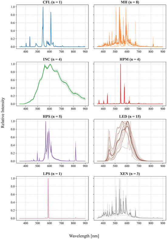
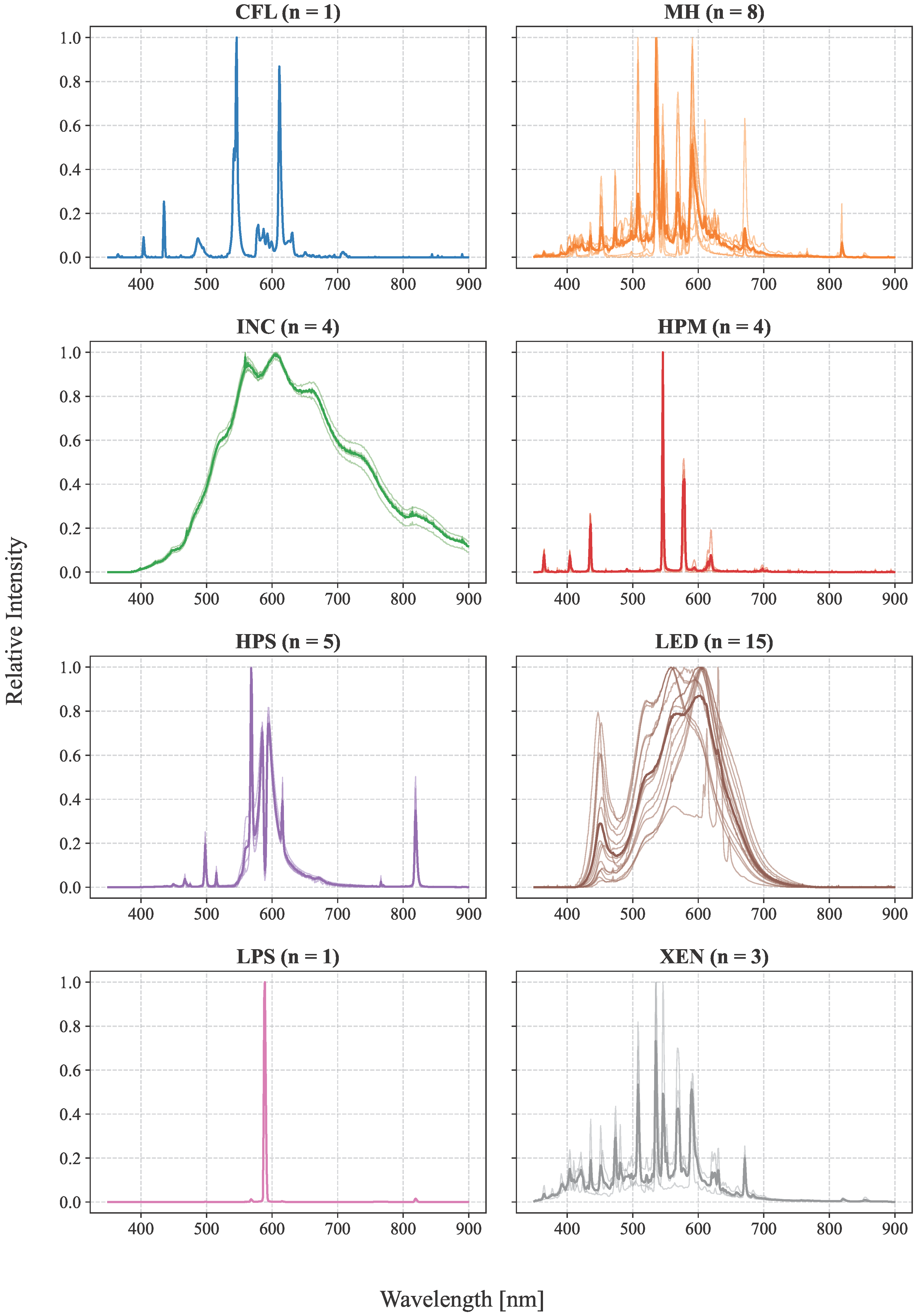
The experimental study is based on a dataset of 41 measured lamp spectra representing commonly used human-made illumination sources, grouped into eight lamp types according to their physical emission characteristics. Each of the 41 lamp spectra was measured individually in a dark, controlled laboratory setting. Lamps were switched on and allowed to reach thermal and optical stabilization prior to measurement, and emission spectra were acquired using two calibrated Ocean Optics spectrometers covering approximately 190 to 880 nm and 375 to 1000 nm, respectively, using a measurement tube fitted with a diffuser. For lamps whose emission spans the ranges of both spectrometers, the two spectra were merged into a single measured spectrum. The distribution of the spectra across the lamp categories is summarized in Table 1, whereas Figure 1 shows their spectral power distributions. The spectra are organized by lamp type, where individual measurements are shown as thin lines and the mean spectrum for each category is highlighted with a thick line. For visualization purposes only, all spectra shown here are normalized to a maximum intensity of 1 to facilitate comparison.

Table 1. Lamp Types and Quantities.

Lamp Type	Subcategory	Description	Number of Lamps
CFL	–	Compact Fluorescent	1
MH	CMH	Ceramic Metal-Halide	2
	QMH	Quartz Metal-Halide	6
INC	INC	Incandescent	1
	HAL	Halogen	3
HPM	–	High-Pressure Mercury	4
HPS	–	High-Pressure Sodium	5
LED	–	Light-Emitting Diode	15
LPS	–	Low-Pressure Sodium	1
XEN	–	Xenon	3
			Total: 41

Figure 1. Normalized SPDs for all 41 light sources, grouped by lamp type. Thick lines indicate the mean spectrum within each category.

Each spectrum can serve either as an endmember in the unmixing process or, when excluded from the endmember matrix, as part of the unknown component. In this study, spectra corresponding to CFL, MH, HPS, and LED lamps are included in the endmember matrix, whereas spectra from INC, HPM, LPS, and XEN lamps are excluded and treated as unknown light sources. This choice reflects realistic illumination conditions: modern public lighting is dominated by LED technology, with HPS, MH, and CFL lamps still present in the existing infrastructure, whereas the remaining lamp types are either significantly less common or largely obsolete. By excluding these sources from the model, we simulate a practical scenario in which the unmixing algorithm operates with an incomplete database and must properly account for contributions that cannot be directly attributed to the available endmembers. It is worth noting that, although unmixing operates on a single representative spectrum per lamp type, the database capturing these categories is built on multiple independent measurements. As shown in Table 1, most categories comprise several lamp units, including up to 15 for LED and 8 for metal-halide lamps. This ensures that both the known and unknown categories account for physical spectral diversity instead of relying on a single arbitrary measurement.

The proposed framework is not restricted to a specific number or choice of spectral channels and can be applied to arbitrary channel configurations depending on the application requirements. In our particular setup, motivated by public area illumination analysis, spectral unmixing is evaluated using a predetermined, fixed configuration consisting of seven spectral channels. These channels were chosen to target the most distinct and stable emission-line features of discharge lamps within the high-sensitivity operating range of the optical detector. This fixed setup is implemented using a combination of optical filters: four narrowband filters with 10 nm full width at half maximum (FWHM) at central wavelengths of 535 nm, 540 nm, 546 nm, and 594 nm; two broader filters with 50 nm FWHM at 525 nm and 650 nm; and one filter with 25 nm FWHM at 575 nm. This channel configuration was previously manually selected based on the specific emission lines of the targeted lamp types and is utilized here as a fixed input for our case study. Although this selection could be further optimized using algorithmic approaches, such an optimization is beyond the scope of this study. Nevertheless, it is important to emphasize that the reference vectors in the endmember matrix $\mathbf{R}$ are never perfectly orthogonal, regardless of the channel configuration chosen. In practice, some degree of correlation among the columns is unavoidable due to the overlapping emission characteristics of the different lamps. As a consequence, any linear unmixing algorithm inherently tends to partially absorb contributions from unknown sources by representing them as linear combinations of endmembers. Despite this correlation, the endmember matrix $\mathbf{R}$ in our setup has a full rank of 4. Furthermore, its condition number is approximately 18.3, confirming that $\mathbf{R}$ remains well-conditioned and satisfies the uniqueness requirement for the QP solution.

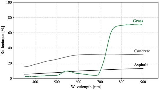
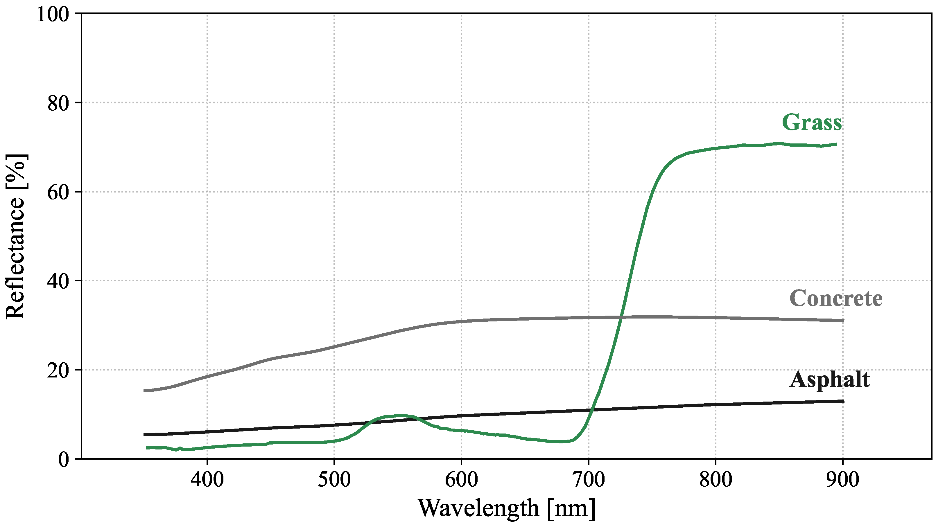
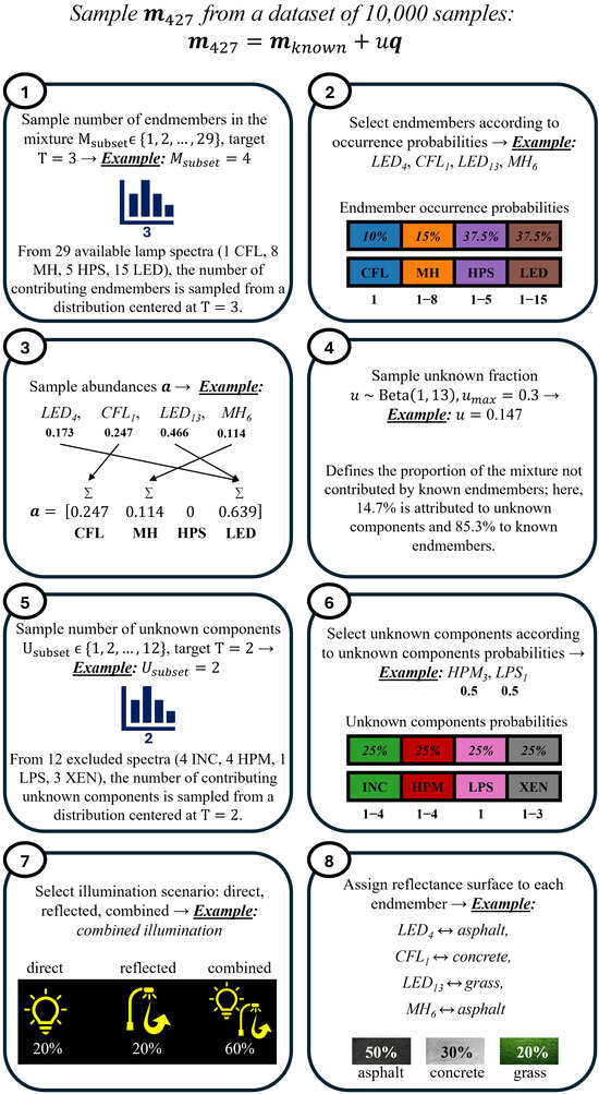
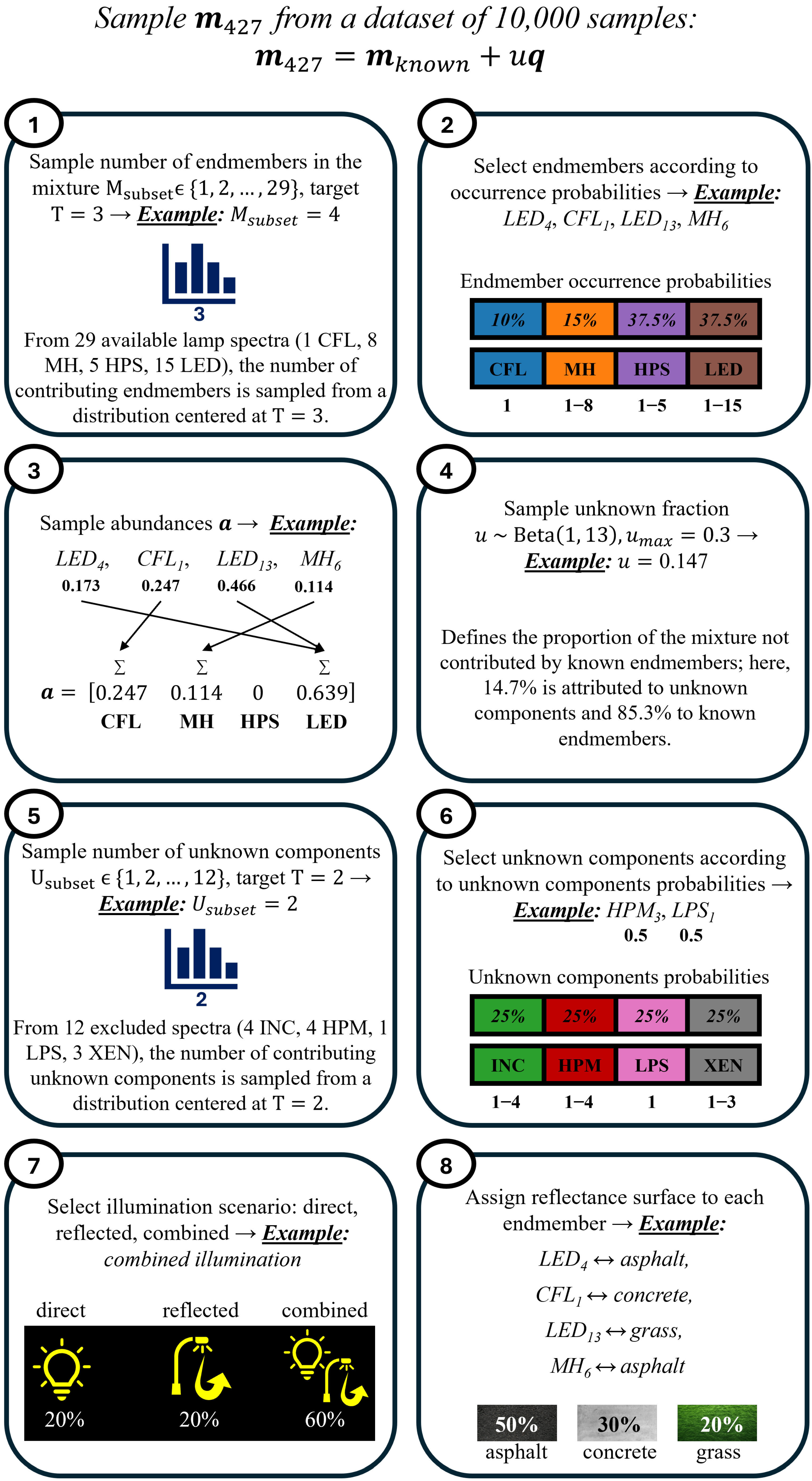
The evaluations are based on the dataset generation procedure described in Section 2.3. The experiments use a dataset of 10,000 generated mixture samples. Each mixture is constructed from a randomly selected subset of endmembers and includes an additional unknown spectral component, whose fractional contribution varies depending on the experiment. Unless otherwise stated, this contribution is governed by a $\mathrm{Beta}(1,13)$ distribution, clipped at $u_{max}=0.3$, corresponding to an expected value of approximately 7.14% and a maximum allowed fraction of 30%. Three illumination scenarios are considered: direct illumination only (20% of the samples), reflected illumination only (20%), and a combination of both (60%). Thus, reflections are present in 80% of the dataset. The individual surface types are sampled with probabilities of 50% for asphalt, 30% for concrete, and 20% for grass or vegetation—a distribution representative of typical outdoor urban environments in which street lighting is deployed. The specific reflectance spectra of the surfaces considered are shown in Figure 2. The occurrence of lamp types is defined to reflect realistic conditions, with LED and HPS lamps having the probability of 37.5% each, followed by MH with 15% and CFL with 10%. The remaining lamp types, which are excluded from the endmember matrix, are assigned equal probabilities of occurrence when forming the unknown component. Figure 3 illustrates the overall generation process. All reported metrics are evaluated as aggregate statistics over the entire dataset. The resulting convex QP is solved in Python 3.13 using the cvxpy 1.7 framework with the ECOS solver at its default settings.

Figure 2. Reflectance spectra of considered surfaces as a function of wavelength [31].

Figure 3. Illustration of the dataset generation process for a single mixture sample based on user-defined parameters.

Experiment 1: Ablation study of the constraint set. To isolate the contribution of each constraint, an ablation study was conducted in which four variants of the QP formulation were evaluated, each employing a different combination of constraints. The evaluated configurations correspond to the classical FCLS formulation (QP₁), its relaxed variant with an inequality sum constraint (QP₂), a version that includes the residual-positivity constraint while retaining the strict equality constraint (QP₃), and finally, the proposed formulation that combines both the relaxed sum constraint and the residual-positivity condition (QP₄). The results are summarized in Table 2. Notably, the third configuration produced infeasible solutions in 15.3% of the tested mixtures, indicating that the combination of a strict sum-to-one constraint with the residual positivity can become unsuitable for mixtures containing unknown contribution. These infeasible optimization solutions were excluded from the reported statistics.

Table 2. Ablation study of the QP formulation with different constraint sets.

Algorithm (Constraints)	${\mathit{RMSE}}_{\mathbf{a}}\downarrow$	${\mathit{RMSE}}_{\mathbf{m}}\downarrow$	$\mathit{KCE}\downarrow$	$\mathit{SAM}\downarrow$	$\mathit{F}1\uparrow$
QP1 ($a_i\ge 0,\sum a_i=1$)	0.1535	0.0391	0.1900	5.1614°	0.7976
QP2 ($a_i\ge 0,\sum a_i\le 1$)	0.1535	0.0391	0.1900	5.1614°	0.7975
QP3 ($a_i\ge 0,\sum a_i=1,\mathbf{m}\ge \mathbf{R}\mathbf{a}$)	0.1564	0.0438	0.2431	4.7532°	0.6822
QP4 ($a_i\ge 0,\sum a_i\le 1,\mathbf{m}\ge \mathbf{R}\mathbf{a}$)	0.1483	0.0376	0.1795	5.3102°	0.8032

Note: QP₃ metrics are computed only over the 84.7% of mixtures for which the solver returned a feasible solution and are therefore not directly comparable to QP₁, QP₂, and QP₄. Bold indicates the best result; arrows show if higher (↑) or lower (↓) is better.

The QP₁ and QP₂ achieve identical performance, which indicates that relaxing the abundance sum constraint alone does not significantly influence the solution when the residual constraint is not present. In contrast, formulation QP₃ leads to degraded performance and infeasible solutions. This behavior arises because the solver is forced to simultaneously satisfy two conflicting requirements: the abundances must sum exactly to one, whereas the reconstructed spectrum of known sources cannot exceed the measured spectrum. In mixtures that contain unknown components, these conditions may become incompatible, which explains both the increase in error and the occurrence of infeasible cases. Although QP₃ achieves the lowest SAM value in this experiment, this is mainly due to the improved alignment of the spectral direction rather than to the better abundance estimation. The combination of a strict sum and residual positivity can bias the reconstruction to match the spectral shape of the measured signal, even when the individual contributions are incorrectly estimated.

The proposed formulation QP₄ consistently achieves the best overall performance across most evaluation metrics. By relaxing the abundance sum constraint while enforcing the residual-positivity condition, the solver can represent mixtures in which a part of the signal originates from sources not included in the endmember matrix. In such cases, the unknown fraction is attributed to the unknown component rather than being redistributed among the known spectra, resulting in improved accuracy. Notably, QP₁ and QP₂ achieve nearly identical performance, indicating that relaxing the sum-to-one constraint alone has very little effect. However, because their strict formulations force the entire measured signal to be explained solely by the known endmembers, both violate the residual-positivity constraint in 29.2% of cases. It means the baseline algorithms frequently attribute more radiant energy to the known lamp types than was physically measured, yielding solutions that are not physically admissible. Enforcing residual positivity without relaxation, as in QP₃, leads to infeasible solutions, thus confirming that both constraints are required. The advantage of the proposed formulation becomes more pronounced as the complexity of the problem increases. In particular, higher levels of reflection, larger unknown contributions, or a larger endmember set further increase the discrepancy between the true mixture and the modeled contribution of the known spectra.

To confirm that this improvement reflects a stable property of the proposed constraint set, the comparison between QP₁ and QP₄ was evaluated across 20 independent runs, with each run utilizing a newly generated set of 10,000 mixtures. This repeated-run validation is restricted to the classical baseline (QP₁) and the fully proposed formulation (QP₄), since QP₂ and QP₃ serve only to isolate the individual constraint effects in Table 2. For each metric, the performance was summarized via the mean and standard deviation computed across the 20 runs. To assess statistical significance, a paired t-test was conducted on the run level differences, supplemented by a 95% confidence interval for the mean difference. Table 3 summarizes these results.

Table 3. Repeated-run comparison of QP₁ and QP₄ over 20 independent runs of 10,000 mixtures each.

Metric	QP1	QP4	95% Confidence Interval	p-Value
$RMS{E}_{\mathbf{a}}$	0.1539 ± 0.0022	0.1484 ± 0.0019	$[-0.0064,-0.0046]$	<0.001
$RMS{E}_{\mathbf{m}}$	0.0392 ± 0.0007	0.0376 ± 0.0007	$[-0.0018,-0.0013]$	<0.001
$KCE$	0.1903 ± 0.0051	0.1797 ± 0.0043	$[-0.0127,-0.0085]$	<0.001
$SAM$	5.160° ± 0.113°	5.308° ± 0.125°	$[+$0.097°, +0.201°]	<0.001
$F1$	0.7954 ± 0.0074	0.8028 ± 0.0053	$[+0.0046,+0.0103]$	<0.001

All five metrics differ between QP₁ and QP₄ with a consistent sign and a small standard deviation relative to the mean difference, and the difference is statistically significant at $p<0.001$ in every case. This indicates that the advantage of the proposed formulation is a reproducible consequence of the constraint set itself. The only metric that slightly increases is SAM. As noted earlier, it measures only the angular alignment of the reconstructed spectrum and is insensitive to whether the underlying abundances are physically admissible. Here, a minor amount of angular fidelity is traded for the physical guarantee that the contribution of known sources never exceeds the measured signal, which represents an acceptable trade-off given the consistent improvement across all other metrics.

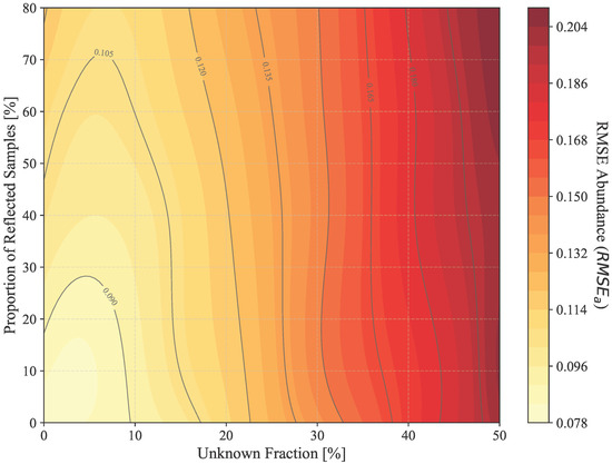
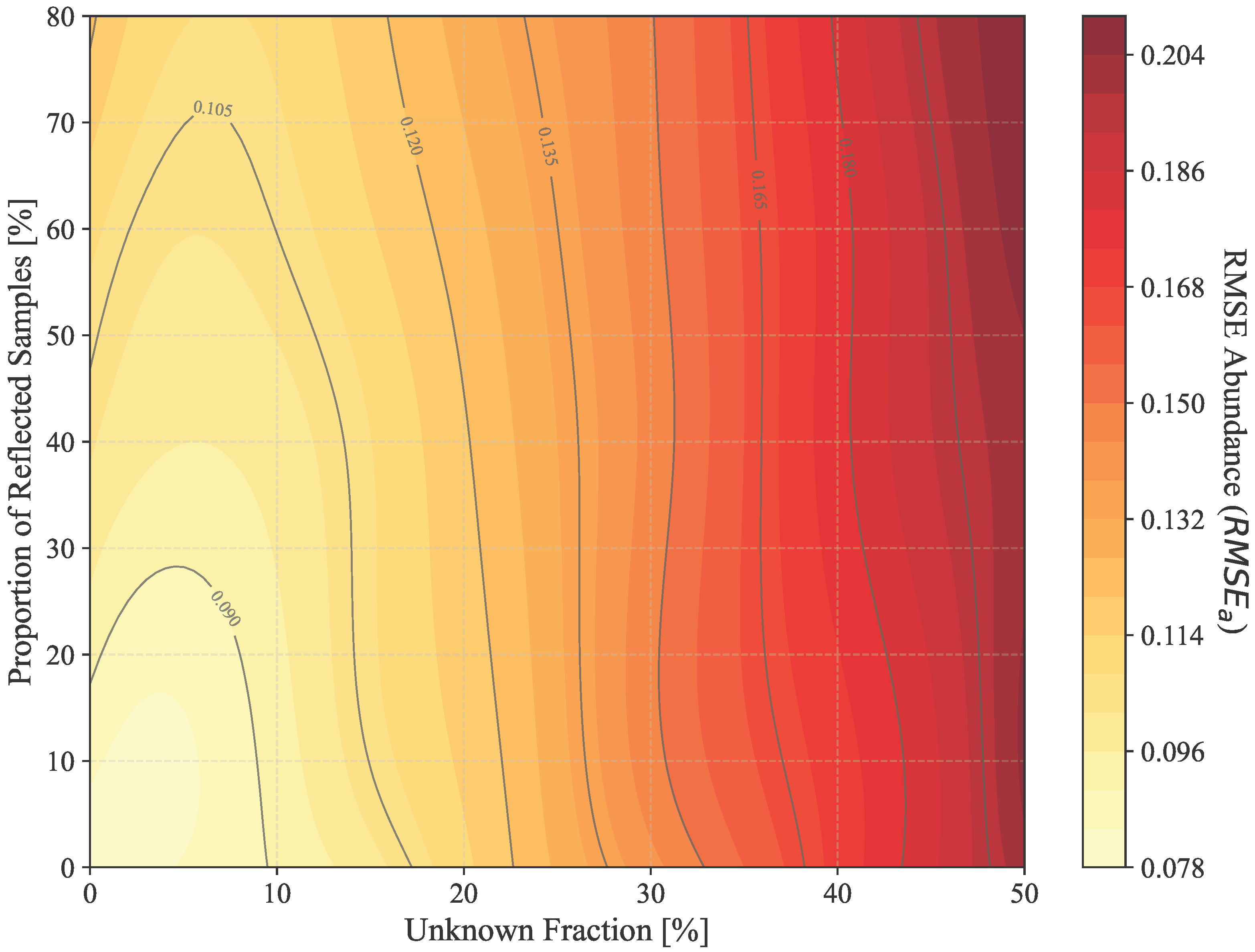
Experiment 2: Impact of unknown contribution and reflections. To evaluate the robustness, an experiment was conducted over a grid of conditions in which two dataset generation parameters were explicitly controlled. Instead of using the default configuration, the unknown contribution in each mixture was set from 0% to 50% in uniform steps, whereas the reflection proportion—defined as the fraction of samples in which reflections are present either in reflected-only or combined illumination scenarios—was varied from 0% to 80%. Spectral unmixing was performed separately for each combination of parameters, and performance was assessed using the metric $RMS{E}_{\mathbf{a}}$. The results are shown in Figure 4, where the horizontal axis represents the unknown fraction, the vertical axis represents the proportion of the reflected samples, and the color scale encodes $RMS{E}_{\mathbf{a}}$. The contour structure reveals that the unmixing performance is highly sensitive to the unknown fraction but comparatively insensitive to the proportion of reflected samples. For unknown contribution levels up to approximately 15%, the method consistently achieves low $RMS{E}_{\mathbf{a}}$ across the full range of reflection conditions, with only minor variation. As the level of unknown contribution increases, the error rises correspondingly, indicating that unknown spectral contributions are the dominant factor directly governing the accuracy of unmixing. This is further confirmed by the shape of the contour lines: at higher unknown contribution levels, the contours become nearly vertical, indicating that $RMS{E}_{\mathbf{a}}$ is largely independent of the reflection proportion for the surface materials, channel configuration, and unknown-source composition considered in this case study.

Figure 4. Robustness of the $RMS{E}_{\mathbf{a}}$ to varying levels of unknown spectral contributions and surface reflections. The near-vertical contours demonstrate the model’s resilience to reflection artifacts.

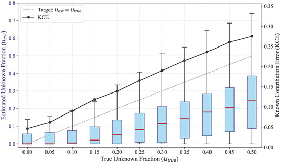
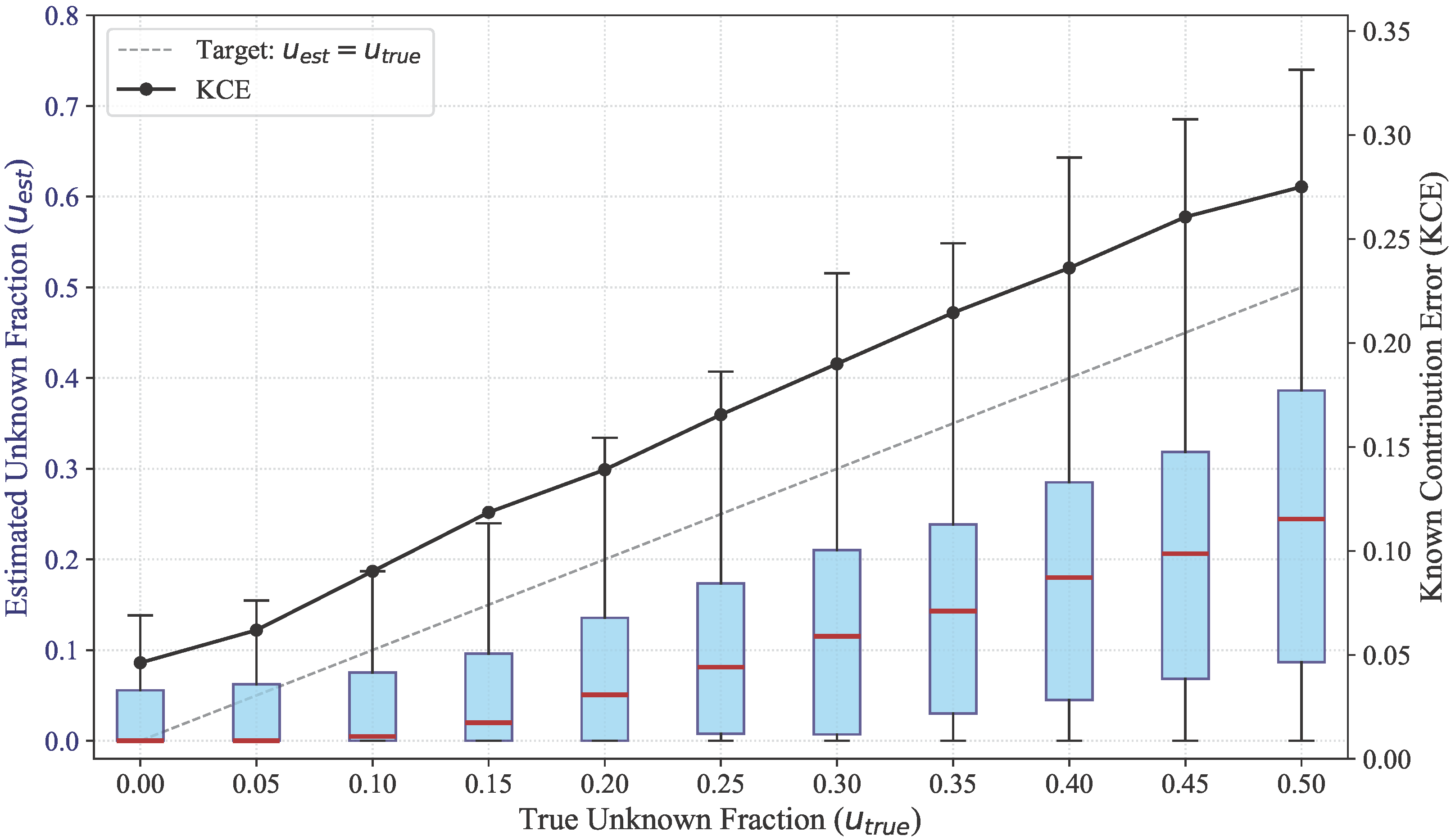
Experiment 3: Detection of unknown spectral contributions. To investigate the ability of the method to detect and quantify unknown components, an experiment was conducted in which the true unknown contribution was explicitly controlled during the dataset generation. The unknown fraction was varied from 0% to 50% in uniform steps, and for each level the estimated unknown contribution $1-{\mathbf{1}}^T{\mathbf{a}}_{est}$ was evaluated across the generated dataset and visualized as a box plot, as shown in Figure 5. The KCE metric was computed at each level of the true unknown contribution and plotted on a secondary vertical axis. Ideally, the estimated unknown fraction would equal the true unknown contribution, yielding a linear relationship along the diagonal. In practice, the estimated contribution grows sublinearly with the true unknown fraction level, indicating that the QP formulation—although capable of detecting the presence of unknown components—tends to underestimate their magnitude. This is an expected consequence of the optimization: the solver attempts to represent the mixture as a linear combination of correlated endmembers before attributing the remainder to the unknown component. The spread of the box plots also reflects this behavior. As the unknown fraction increases, the spread grows substantially, reflecting the greater variability arising from the difficulty of distinguishing unknown spectral components from combinations of known lamp spectra. The KCE metric closely follows the same trend: it increases progressively as the discrepancy between the true and estimated contributions becomes more pronounced.

Figure 5. Relationship between true and estimated unknown spectral fractions. Box plots (median and interquartile range) illustrate estimation variability at each level; the secondary axis shows the corresponding KCE trend.

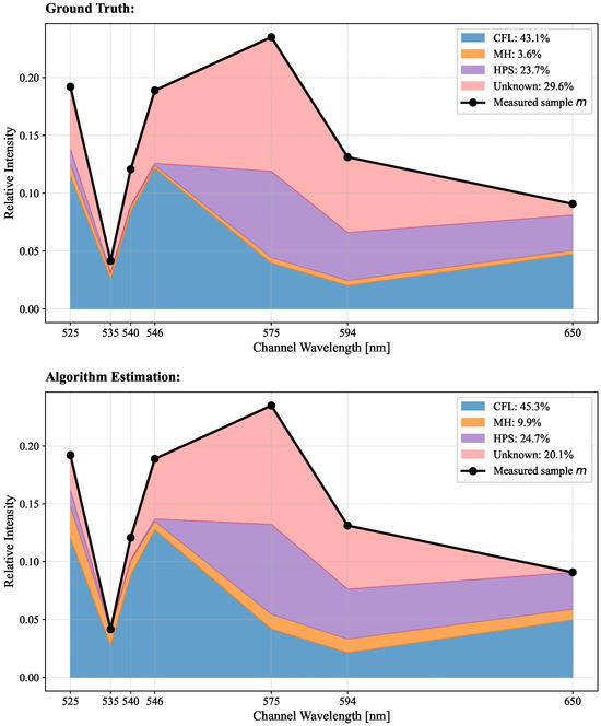
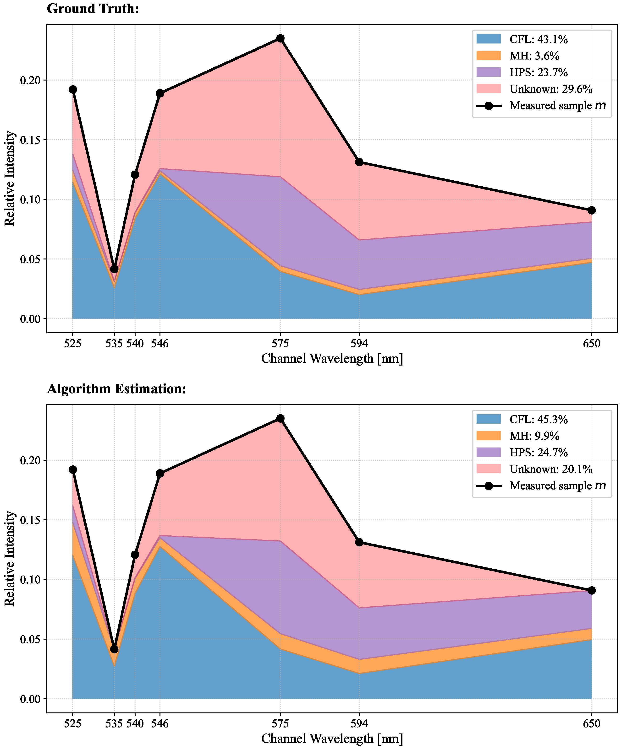
Experiment 4: Effect of the proposed constraints. Figure 6 shows a representative spectral mixture of the dataset, with the horizontal axis corresponding to the selected spectral channels and the vertical axis showing normalized intensity values. The measured spectrum is displayed as a continuous curve, with the contributions of individual lamp types shown below. The left side of the figure shows the true composition of the mixture, including both the known lamp contributions and unknown component. The right side shows the abundance estimates produced by the QP algorithm. In this example, the algorithm correctly identifies the endmembers and assigns appropriate contributions to each. Importantly, it also recognizes that the mixture cannot be fully explained by known endmembers alone, and assigns a non-zero value to the unknown component. Although the estimated unknown fraction (20.1% in this example) is lower than the true value (29.6% in this example), it is still capable of representing the presence of an unknown component rather than forcing it to be absorbed by known spectra. Under the strict equality constraint, the entire unknown contribution would necessarily be redistributed among the known lamp types, leading to systematically biased abundance estimates and potentially incorrect identification of the present endmembers. The residual-positivity constraint ensures that the measured spectrum remains greater than or equal to the total modeled contribution of the known endmembers in every spectral band. This is evident in the figure where the sum of the known contributions never exceeds the measured signal in any channel. When an unknown component is included, the reconstructed spectrum matches the measured signal. For example, in the channel centered at 535 nm, the algorithm assigns no unknown contribution; nevertheless, the constraint guarantees that the summed contribution of the known endmembers alone does not exceed the measurement in that band, thus preserving the physical consistency of the solution.

Figure 6. Ground-truth decomposition and corresponding algorithm estimation for a representative spectral mixture.

4. Conclusions

This study presents a QP framework for spectral unmixing that incorporates a physically motivated set of constraints to better handle mixtures containing unknown spectral components. By introducing a residual-positivity constraint and relaxing the abundance sum constraint from strict equality to inequality, the model can explicitly account for contributions not represented in the known endmember library. The ablation study confirms that neither modification alone is sufficient: relaxing the sum constraint without the residual-positivity condition yields no improvement over the standard FCLS, whereas enforcing residual positivity under strict equality produces infeasible solutions in a substantial fraction of cases. Only their combination, as in the proposed QP₄ formulation, consistently improves abundance estimation accuracy, reconstruction quality, and endmember detection reliability in the evaluated conditions. Importantly, this is achieved without introducing any regularization hyperparameters or stochastic optimization, and the resulting solution is unique whenever the endmember library has linearly independent spectra, as verified for the case study considered here.

In addition, a flexible dataset generation framework based on the GLMM is developed to enable controlled and physically consistent evaluation. The framework explicitly models surface reflections through band-dependent scaling of endmember spectra and supports parametric control over the number of endmembers, their occurrence probabilities, and the magnitude and type of unknown spectral components. This level of control is difficult to achieve with real measurements, where ground-truth abundance information is rarely available. The framework is general and is not tied to the proposed method, making it directly applicable to alternative spectral unmixing approaches across a wide range of problem settings.

The experimental results reveal that unmixing performance is strongly sensitive to the magnitude of unknown spectral contributions, yet comparatively robust to the proportion of reflected samples under the surface materials, seven-channel configuration, and data-generation settings considered in this study—even when reflections are present in up to 80% of the dataset. The detection and quantification of unknown components remain inherently challenging: the estimated unknown fraction grows sublinearly with the true value because the solver tends to explain as much of the observed signal as possible using the available endmembers before attributing the remainder to an unknown component. This behavior is quantified using the proposed KCE metric, which tracks the discrepancy between the true and estimated total known contributions as a function of the unknown fraction level.

The proposed framework is not restricted to the specific channel configuration or database of light sources used in this study. Although seven spectral channels, implemented through a combination of narrowband and broader optical filters, were selected to match the outdoor lighting application, both the QP formulation and the dataset generation procedure do not depend on the number and choice of spectral channels. Consequently, these components can be adapted to different configurations, broader spectral ranges, and application domains beyond public area illumination analysis.

Overall, the proposed approach provides both a robust optimization formulation and a generalizable dataset generation framework, which is particularly valuable in scenarios where the endmember library is incomplete and in-situ measurements are limited or impractical. Since a real ground truth dataset for mixed nighttime illumination is not available, our quantitative results describe the performance of the method under the generative assumptions detailed throughout this work. These results characterize the behavior of the algorithm under physically motivated simulations rather than demonstrating generalization to real outdoor lighting conditions. Future work will focus on using this framework to explore adaptive channel selection strategies, guided by quantitative criteria such as A-, D-, and E-optimality, condition number, and inter-endmember correlation, that improve separability among highly correlated source spectra. In addition, the approach will be validated against real-world spectral measurements collected under controlled outdoor conditions.

References

- Keshava, N.; Mustard, J. Spectral unmixing. IEEE Signal Process. Mag. 2002, 19, 44–57. [Google Scholar] [CrossRef] [Scilit]
- Bioucas-Dias, J.M.; Plaza, A.; Dobigeon, N.; Parente, M.; Du, Q.; Gader, P.; Chanussot, J. Hyperspectral unmixing overview: Geometrical, statistical, and sparse regression-based approaches. IEEE J. Sel. Top. Appl. Earth Obs. Remote Sens. 2012, 5, 354–379. [Google Scholar] [CrossRef] [Scilit]
- Somers, B.; Asner, G.P.; Tits, L.; Coppin, P. Endmember variability in Spectral Mixture Analysis: A review. Remote Sens. Environ. 2011, 115, 1603–1616. [Google Scholar] [CrossRef] [Scilit]
- Li, C.; Zhu, D.; Wu, C. Spatial–Spectral Graph Convolutional Network for Hyperspectral Target Detection. IEEE Geosci. Remote Sens. Lett. 2025, 22, 5510305. [Google Scholar] [CrossRef] [Scilit]
- Black, D.; Liquet, B.; Ieva, A.D.; Stummer, W.; Molina, E.S. Spectral library and method for sparse unmixing of hyperspectral images in fluorescence guided resection of brain tumors. Biomed. Opt. Express 2024, 15, 4406–4424. [Google Scholar] [CrossRef] [Scilit] [PubMed]
- Adams, J.B.; Smith, M.O.; Johnson, P.E. Spectral mixture modeling: A new analysis of rock and soil types at the Viking Lander 1 site. J. Geophys. Res. Solid Earth 1986, 91, 8098–8112. [Google Scholar] [CrossRef] [Scilit]
- Bioucas-Dias, J.M.; Figueiredo, M.A.T. Alternating Direction Algorithms for Constrained Sparse Regression: Application to Hyperspectral Unmixing. arXiv 2012, arXiv:1002.4527. [Google Scholar]
- Parente, M.; Iordache, M.D. Sparse Unmixing of Hyperspectral Data: The Legacy of SUnSAL. In 2021 IEEE International Geoscience and Remote Sensing Symposium IGARSS; IEEE: Piscataway, NJ, USA, 2021; pp. 21–24. [Google Scholar] [CrossRef] [Scilit]
- Eismann, M.T.; Hardie, R.C. Stochastic spectral unmixing with enhanced endmember class separation. Appl. Opt. 2004, 43, 6596–6608. [Google Scholar] [CrossRef] [Scilit] [PubMed]
- Dobigeon, N.; Moussaoui, S.; Coulon, M.; Tourneret, J.Y.; Hero, A. Joint Bayesian Endmember Extraction and Linear Unmixing for Hyperspectral Imagery. IEEE Trans. Signal Process. 2009, 57, 4355–4368. [Google Scholar] [CrossRef] [Scilit]
- Guo, R.; Wang, W.; Qi, H. Hyperspectral image unmixing using autoencoder cascade. In 2015 7th Workshop on Hyperspectral Image and Signal Processing: Evolution in Remote Sensing (WHISPERS); IEEE: Piscataway, NJ, USA, 2015; pp. 1–4. [Google Scholar] [CrossRef] [Scilit]
- Palsson, B.; Sigurdsson, J.; Sveinsson, J.R.; Ulfarsson, M.O. Hyperspectral Unmixing Using a Neural Network Autoencoder. IEEE Access 2018, 6, 25646–25656. [Google Scholar] [CrossRef] [Scilit]
- Hu, J.; Wang, T.; Jin, Q.; Peng, C.; Liu, Q. A multi-domain dual-stream network for hyperspectral unmixing. Int. J. Appl. Earth Obs. Geoinf. 2024, 135, 104247. [Google Scholar] [CrossRef] [Scilit]
- Su, L.; Liu, J.; Yuan, Y.; Chen, Q. A Multi-Attention Autoencoder for Hyperspectral Unmixing Based on the Extended Linear Mixing Model. Remote Sens. 2023, 15, 2898. [Google Scholar] [CrossRef] [Scilit]
- Chen, X.; Meng, F.; Mo, Y.; Sun, H. Spatial-spectral collaborative attention network for hyperspectral unmixing. Geocarto Int. 2024, 39, 2417919. [Google Scholar] [CrossRef] [Scilit]
- Bhatt, J.S.; Joshi, M.V. Deep Learning in Hyperspectral Unmixing: A Review. In IGARSS 2020–2020 IEEE International Geoscience and Remote Sensing Symposium; IEEE: Piscataway, NJ, USA, 2020; pp. 2189–2192. [Google Scholar] [CrossRef] [Scilit]
- Harsanyi, J.; Chang, C.I. Hyperspectral image classification and dimensionality reduction: An orthogonal subspace projection approach. IEEE Trans. Geosci. Remote Sens. 1994, 32, 779–785. [Google Scholar] [CrossRef] [Scilit]
- Dong, L.; Lu, X.; Liu, G.; Yuan, Y. A Novel NMF Guided for Hyperspectral Unmixing From Incomplete and Noisy Data. IEEE Trans. Geosci. Remote Sens. 2022, 60, 5513515. [Google Scholar] [CrossRef] [Scilit]
- Halimi, A.; Bioucas-Dias, J.M.; Dobigeon, N.; Buller, G.S.; McLaughlin, S. Fast Hyperspectral Unmixing in Presence of Nonlinearity or Mismodeling Effects. IEEE Trans. Comput. Imaging 2017, 3, 146–159. [Google Scholar] [CrossRef] [Scilit]
- Li, C.; Ma, Y.; Mei, X.; Liu, C.; Ma, J. Hyperspectral Unmixing with Robust Collaborative Sparse Regression. Remote Sens. 2016, 8, 588. [Google Scholar] [CrossRef] [Scilit]
- Chang, C.I. Target Abundance-Constrained Subpixel Detection: Partially Constrained Least-Squares Methods. In Hyperspectral Imaging; Springer: Boston, MA, USA, 2003; pp. 39–50. [Google Scholar] [CrossRef] [Scilit]
- Drumetz, L.; Veganzones, M.A.; Henrot, S.; Phlypo, R.; Chanussot, J.; Jutten, C. Blind Hyperspectral Unmixing Using an Extended Linear Mixing Model to Address Spectral Variability. IEEE Trans. Image Process. 2016, 25, 3890–3905. [Google Scholar] [CrossRef] [Scilit] [PubMed]
- Hong, D.; Yokoya, N.; Chanussot, J.; Zhu, X.X. An Augmented Linear Mixing Model to Address Spectral Variability for Hyperspectral Unmixing. IEEE Trans. Image Process. 2019, 28, 1923–1938. [Google Scholar] [CrossRef] [Scilit] [PubMed]
- Hua, Z.; Li, X.; Chen, S.; Zhao, L. Hyperspectral unmixing with scaled and perturbed linear mixing model to address spectral variability. J. Appl. Remote Sens. 2020, 14, 026515. [Google Scholar] [CrossRef] [Scilit]
- Cheng, Y.; Zhao, L.; Chen, S.; Li, X. Hyperspectral Unmixing Network Accounting for Spectral Variability Based on a Modified Scaled and a Perturbed Linear Mixing Model. Remote Sens. 2023, 15, 3890. [Google Scholar] [CrossRef] [Scilit]
- Imbiriba, T.; Borsoi, R.A.; Bermudez, J.C.M. Generalized linear mixing model accounting for endmember variability. arXiv 2017, arXiv:1710.07723. [Google Scholar]
- Borsoi, R.A.; Imbiriba, T.; Bermudez, J.C.M.; Richard, C.; Chanussot, J.; Drumetz, L.; Tourneret, J.Y.; Zare, A.; Jutten, C. Spectral Variability in Hyperspectral Data Unmixing: A comprehensive review. IEEE Geosci. Remote Sens. Mag. 2021, 9, 223–270. [Google Scholar] [CrossRef] [Scilit]
- Zhao, M.; Chen, J.; He, Z. A laboratory-created dataset with ground-truth for hyperspectral unmixing evaluation. arXiv 2019, arXiv:1902.08347. [Google Scholar]
- Paura, V.; Marcinkevičius, V. Benchmark for Hyperspectral Unmixing Algorithm Evaluation. Informatica 2023, 34, 285–315. [Google Scholar] [CrossRef] [Scilit]
- Palsson, B.; Ulfarsson, M.O.; Sveinsson, J.R. Synthesis of Synthetic Hyperspectral Images with Controllable Spectral Variability Using a Generative Adversarial Network. Remote Sens. 2023, 15, 3919. [Google Scholar] [CrossRef] [Scilit]
- Kokaly, R.F.; Clark, R.N.; Swayze, G.A.; Livo, K.E.; Hoefen, T.M.; Pearson, N.C.; Wise, R.A.; Benzel, W.M.; Lowers, H.A.; Driscoll, R.L.; et al. USGS Spectral Library Version 7; Technical Report; U.S. Geological Survey: Reston, VA, USA, 2017. [Google Scholar]
- Heinz, D.; Chein-I-Chang. Fully constrained least squares linear spectral mixture analysis method for material quantification in hyperspectral imagery. IEEE Trans. Geosci. Remote Sens. 2001, 39, 529–545. [Google Scholar] [CrossRef] [Scilit]
- Boyd, S.; Vandenberghe, L. Convex Optimization; Cambridge University Press: Cambridge, UK, 2004. [Google Scholar]
- Kruse, F.; Lefkoff, A.; Boardman, J.; Heidebrecht, K.; Shapiro, A.; Barloon, P.; Goetz, A. The spectral image processing system (SIPS)—interactive visualization and analysis of imaging spectrometer data. Remote Sens. Environ. 1993, 44, 145–163. [Google Scholar] [CrossRef] [Scilit]
- Zhang, J.; Geng, W.; Liang, X.; Li, J.; Zhuo, L.; Zhou, Q. Hyperspectral remote sensing image retrieval system using spectral and texture features. Appl. Opt. 2017, 56, 4785–4796. [Google Scholar] [CrossRef] [Scilit] [PubMed]
Disclaimer/Publisher’s Note: The statements, opinions and data contained in all publications are solely those of the individual author(s) and contributor(s) and not of MDPI and/or the editor(s). MDPI and/or the editor(s) disclaim responsibility for any injury to people or property resulting from any ideas, methods, instructions or products referred to in the content. |
© 2026 by the authors. Licensee MDPI, Basel, Switzerland. This article is an open access article distributed under the terms and conditions of the Creative Commons Attribution (CC BY) license.