


Highlights
What are the main findings?
- The OY, WLS, and ELS show distinct January–April variability: only the OY has a significant accumulated-area increase, the WLS has the strongest episodic variability and most frequent large-area events, and the ELS has the clearest late-season maximum.
- NW shows the strongest same-day or one-day-leading association with daily polynya area. HP apportions the explained variance among covarying predictors; SST, T2M, and SIT also account for substantial shares that vary by region and timescale.
What are the implications of the main findings?
- Neighboring Kara–Laptev polynyas should not be treated as one uniform system because coastline orientation, landfast-ice geometry, and background ice–ocean conditions shape their responses differently.
- Changes in offshore-wind patterns, atmospheric and oceanic conditions, and sea-ice thickness may be associated with altered winter–spring polynya activity, with implications for air–sea exchange, sea-ice production, and Arctic navigation windows.
Abstract
Coastal polynyas in the Kara–Laptev Seas regulate winter air–sea exchange and sea-ice production, but neighboring polynya systems can behave differently. This study examines January–April variability of the Ob–Yenisey (OY), western Laptev Sea (WLS), and eastern Laptev Sea (ELS) polynyas from 2003 to 2025 using passive-microwave sea-ice concentration, ERA5 winds and air temperature, AMSR-MPR sea-surface temperature, TOPAZ4b sea-ice thickness, and AO/ENSO indices. The three regions show distinct spatiotemporal variations. The OY exhibits the only significant increase in accumulated polynya area (+1.72 × 10⁴ km2 day a−1), the WLS has the largest interannual variability and the most frequent large-area events, and the ELS is most strongly concentrated in late March and April. NW has the clearest same-day or one-day-lead association with opening, consistent with wind-driven mechanical divergence, while coastline orientation and landfast-ice geometry are associated with differences in regional responses. Hierarchical partitioning (HP) assigns the largest daily relative statistical allocation to SST in the WLS and ELS; because this association is predominantly synchronous, it is interpreted as an ice–ocean state relationship rather than as a demonstrated antecedent control. Annual associations are more region dependent and include NW, T2M, SST, and SIT. AO is positively correlated with polynya activity, whereas ENSO has no consistent relationship.
1. Introduction
The Arctic responds strongly to climate change, and changes in sea-ice cover feed back on the climate system [1]. Polynyas are recurring areas of open water or thin ice within the sea-ice pack, where the ocean, ice, and atmosphere remain tightly coupled [2,3]. In winter and early spring, coastal polynyas are especially active sites of heat and moisture exchange, new ice formation, brine rejection, and shelf-water modification [3,4]. They also influence regional ecosystems and can affect the timing and efficiency of Arctic navigation.
Coastal-polynya opening has commonly been associated with offshore winds that move landfast or drifting ice away from the coast [2,5,6]. This physical mechanism motivates evaluation of the timing and orientation of local winds, but wind alone does not account for the observed regional differences in area, persistence, and interannual variability [7,8,9,10]. The same wind event can coincide with different ice-divergence responses depending on coastline orientation, landfast-ice configuration, ice thickness, air temperature, and the oceanic thermal background.
The Kara–Laptev Seas are well suited for examining these coupled regional conditions. Three recurrent coastal-polynya systems occur in this sector: the Ob–Yenisey (OY) polynya in the southern Kara Sea, the western Laptev Sea (WLS) polynya, and the eastern Laptev Sea (ELS) polynya [11,12,13]. These geographically close regions differ in coastline orientation, prevailing offshore-wind orientation, sea-ice thickness, and oceanic thermal setting. Previous work has documented active sea-ice production in Siberian shelf polynyas [4,11,12,14].
Previous studies have examined polynyas in individual Arctic regions, but a consistent comparison across the neighboring OY, WLS, and ELS systems remains limited [14,15,16]. In particular, wind-related associations and background thermal or ice-state associations have not been evaluated in a unified framework. This gap matters because nearby polynyas can respond asynchronously to similar large-scale atmospheric circulation, especially when local coastline geometry changes the effective offshore wind. Long-term passive-microwave sea-ice concentration products now make such a regional comparison possible [17,18,19].
Here, we examine the spatiotemporal variability and environmental associations of coastal polynyas in the Kara–Laptev Seas from 2003 to 2025, focusing on the OY, WLS, and ELS. We test whether offshore wind shows the timing and statistical association expected of an immediate dynamical trigger, while T2M, SST, and SIT are associated with the magnitude and persistence of the response. The objectives are to: (1) map recurrent coastal-polynya occurrence from passive-microwave SIC; (2) quantify daily January–April evolution and interannual accumulated-area variability; and (3) compare regional associations with offshore wind, T2M, SST, and SIT. River runoff is considered only as a possible background influence because its winter association is indirect and mediated by stratification, mixing, advection, and ice cover.
2. Materials and Methods
2.1. Study Region and Data
Daily sea-ice concentration (SIC) was obtained from the University of Bremen AMSR-E/AMSR2 passive-microwave products at 6.25 km spatial resolution [20]. This record, available continuously since summer 2002, is currently the longest relatively high-resolution passive-microwave time series suitable for examining long-term polynya variability. Because AMSR-E data are unavailable for January–April 2012, that winter was filled using SSMIS/DMSP SIC at the same spatial resolution. Both products use the ARTIST Sea Ice (ASI) algorithm [21,22,23]. To reduce sensor-transition effects, the 2012 SSMIS estimates were corrected using regression relationships with adjacent ASI-based records [24]. The corrected series preserved the main coastal-polynya patterns and area estimates near the 75% SIC threshold; details of the bias correction and continuity check are given in Figure S1.
In addition to SIC, sea-surface temperature (SST) was obtained from the Multi-parameter Retrieval (MPR) product of the Institute of Environmental Physics, University of Bremen (IUP), to represent the oceanic thermal background of the ice–ocean system [25]. The MPR product is derived from passive-microwave brightness temperatures using an optimal-estimation method and is provided as daily NetCDF data on a 25 km EASE-Grid for the Arctic freezing season, spanning the AMSR-E and AMSR2 sensor periods. Surface temperature from the MPR product was compared with 2 m air temperature (Figure S2).
Sea-ice thickness (SIT) was obtained from the Copernicus Marine Service Arctic Ocean Physics Reanalysis produced by the Nansen Environmental and Remote Sensing Center (NERSC) [26]. TOPAZ4b is a coupled sea-ice–ocean assimilation product based on HYCOM and a Deterministic Ensemble Kalman Filter [27]. Long-term Arctic SIT observations and reanalyses are subject to retrieval and model uncertainty [28,29]. TOPAZ4b was therefore used here only to characterize regional sea-ice conditions in the OY, WLS, and ELS.
Meteorological variables were taken from ERA5 at 0.25° × 0.25° spatial resolution and hourly temporal resolution [30]. The 10 m zonal and meridional winds were used to describe dynamic forcing, and 2 m air temperature (T2M) was used to represent atmospheric thermal conditions that may affect ice growth, ice stability, and sensitivity to wind forcing. All meteorological fields were averaged to daily values and interpolated to the SIC grid where required.
The Arctic Oscillation (AO) index and the Niño 3.4 index were obtained from the NOAA Physical Sciences Laboratory (PSL) [31,32]. The AO index represents the oscillation of atmospheric pressure between the Arctic and mid-latitudes and serves as a key indicator of winter climate variability in the Northern Hemisphere [33]. The Niño 3.4 index represents sea-surface temperature anomalies averaged over 5°N–5°S, 170°W–120°W, and is widely used to describe the state of the El Niño–Southern Oscillation (ENSO) [34]. In this study, AO and ENSO are not treated as direct forcing factors for coastal-polynya opening. Instead, they are considered large-scale circulation modes that may indirectly affect regional wind patterns, air temperature, and background sea-ice conditions. They were used only as exploratory large-scale context and not to infer climate cycles or teleconnection mechanisms.
Daily river discharge records for the Ob, Yenisey, and Lena Rivers for 2003–2024 were obtained from the Arctic Great Rivers Observatory (ArcticGRO) and used only to support the background discussion of possible river-runoff influence [35].
The date 29 February was excluded from all daily environmental analyses to ensure a uniform 365-day calendar treatment. The merged polynya-area record was unavailable on five additional dates—3–4 February 2010 and 19–21 April 2019—so analyses requiring area data omitted those dates. At zero lead, the univariate offshore-wind, T2M, and SIT analyses use n = 2755. The SST analysis uses n = 2635 because SST is unavailable throughout 2012. The complete-case five-predictor daily models likewise use n = 2635; 2012 is omitted because of the SST gap, and 29 February is excluded in all remaining years.
In the analysis, SIC was used to identify candidate polynyas; ERA5 winds characterized local wind conditions; ERA5 T2M, AMSR-MPR SST and surface temperature, and TOPAZ4b SIT described the background atmosphere–ice–ocean state; and AO/ENSO indices provided large-scale circulation context. Dataset sources and preprocessing steps are summarized in Table S1.
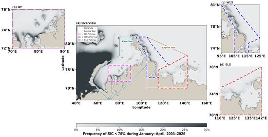
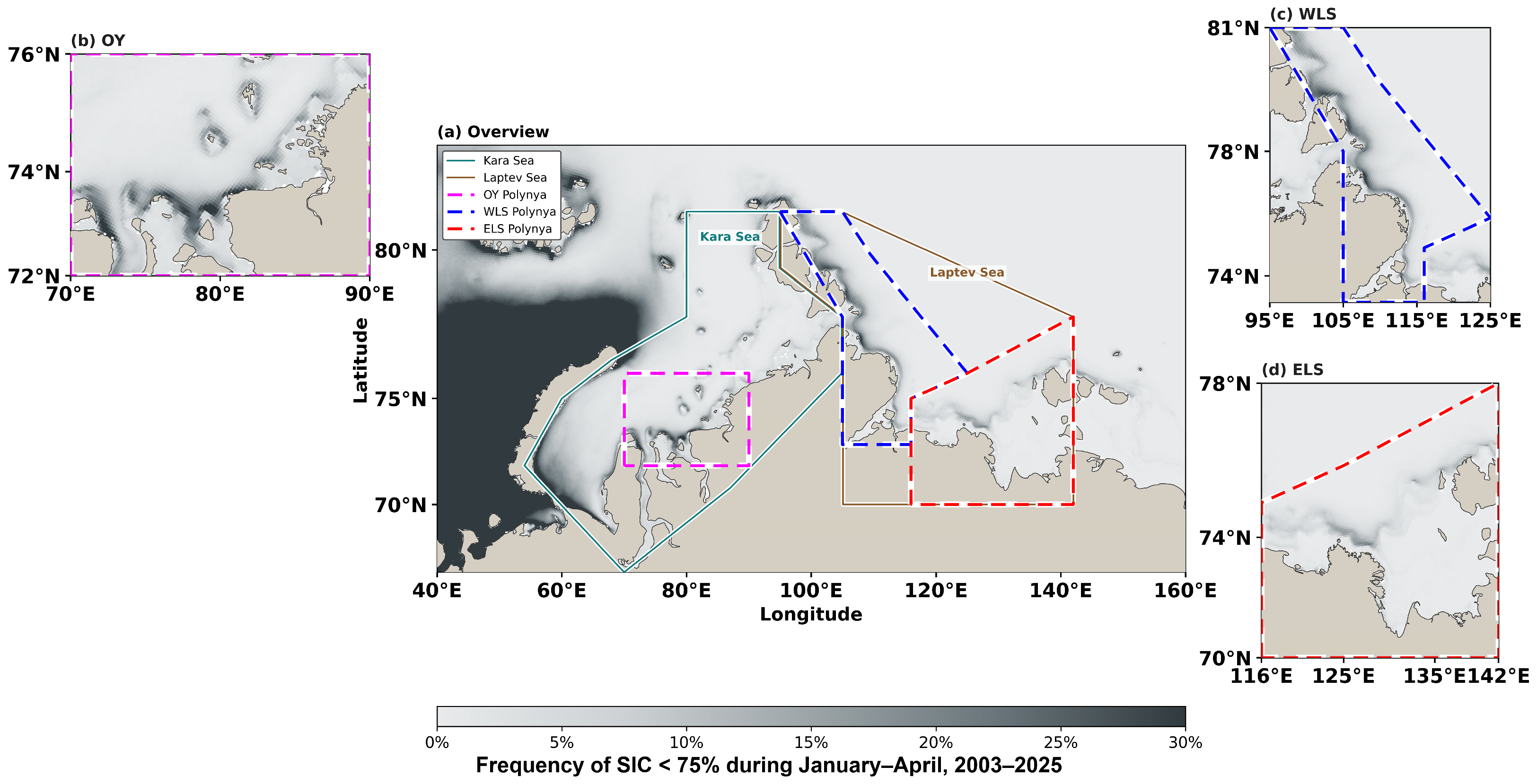
As shown in Table 1 and Figure 1, the OY polynya lies in the southern Kara Sea near the Ob and Yenisey River mouths, approximately between 70°E–90°E and 72°N–76°N. The WLS occupies the western Laptev Sea, approximately between 95°E–125°E and 73°N–81°N, east of the Taimyr Peninsula and Severnaya Zemlya. The ELS lies in the eastern Laptev Sea near the Lena River mouth, approximately between 116°E–142°E and 70°N–78°N. The systems are geographically adjacent but differ in coastline orientation, associated offshore-wind direction, landfast-ice configuration, sea-ice thickness, and oceanic thermal background. These regional characteristics provide the geographic context for the comparative analyses below.
Table 1.
Geographic characteristics of the OY, WLS, and ELS coastal-polynya study regions.
Figure 1.
Spatial distribution of coastal-polynya occurrence frequency in the Kara–Laptev Seas during January–April, 2003–2025. The grayscale basemap shows the percentage of valid daily observations in which each grid cell was identified as a coastal polynya (SIC < 75%). The OY, WLS, and ELS analysis regions are indicated by high-contrast magenta, blue, and red dashed outlines, respectively, with black under-strokes. Kara Sea and Laptev Sea boundaries and labels are included for geographic reference. Panel (a) provides the regional overview, while panels (b–d) show enlarged OY, WLS, and ELS views.
2.2. Methods
Polynya candidates were identified on the SIC grid using a 75% threshold, following previous passive-microwave studies of Arctic coastal polynyas [23,36,37,38]. Cells with SIC < 75% were treated as open-water or thin-ice candidates, whereas cells with SIC ≥ 75% were treated as sea ice. The baseline threshold of 75% was selected to identify pixels containing substantial open water or thin ice while avoiding an overly restrictive definition that would retain only extensively open-water conditions. Sensitivity tests using thresholds of 50%, 60%, 70%, 75%, and 80% produced broadly similar occurrence-frequency and accumulated-area patterns (Figures S3 and S4). Comparisons with a 1 km MODIS–AMSR2 merged SIC product, available since 2017, preserved the main spatial patterns for the three retained case dates (Figure S5; Table S2). Because its record is comparatively short, this product is used only as a spatial reference rather than as a validation dataset. To assess the effect of the operational filters, a complete 3 × 3 × 2 detection-sensitivity matrix was computed from the original daily SIC grids (Table S3; Figure S17): three SIC thresholds (50%, 75%, 80%) and three region-specific patch-size quantiles (Q50, Q75, Q90), each with and without the late-April persistence screen. The SIC 75% × Q75 settings reproduced the pre-screened and final daily-area reference series exactly (maximum daily difference 0 km2). Across all 18 configurations, the WLS > ELS > OY regional ranking and the signs of the NW, T2M, SST, and SIT associations were retained, and the OY accumulated-area trend remained positive (0.49–2.44 × 10⁴ km2 day a−1) and significant (HAC, p < 0.05) in 17 of 18 configurations; the single exception was the most restrictive combination (SIC 50%, Q90, no persistence screen), in which the OY trend remained positive but was not significant (p = 0.084).
The analysis was limited to January–April. In November–December, the coastal ice edge and landfast-ice boundary are still developing, while winter conditions become more stable after January (Figure S6) [8,9,10]. April was retained because polynya activity remains frequent before widespread melt. However, low-SIC water in late April is more likely to include seasonal open-water expansion, as the T2M begins to exceed the ice-surface temperature around 20 April (Figure S2). Ice-free areas connected to the open ocean, such as those near Novaya Zemlya under Atlantic-origin warm-water influence, were excluded because they do not represent coastal latent-heat polynyas.
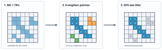
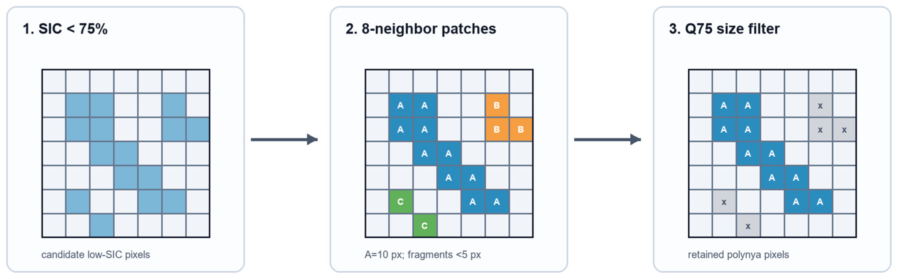
Polynya detection occasionally produces sporadic, isolated low-SIC cells. At the 6.25 km grid scale, such disconnected one- or two-pixel cells may arise from retrieval uncertainty, mixed-pixel effects, or short-lived openings, and they do not represent a spatially coherent regional polynya structure; they are therefore treated as noise and removed. As shown in Figure 2, neighboring SIC < 75% cells were first grouped within each predefined region using eight-neighbor adjacency, after which a region-specific Q75 patch-size criterion was applied. Using region-specific quantiles avoids imposing a single absolute area threshold on three regions with different coastal geometry and typical polynya scales. For each region, non-zero low-SIC patch areas were ranked in ascending order, and the 75th percentile (Q75) was used as the minimum retained patch area: 8 cells (312.5 km2) for the OY and WLS and 5 cells (195.3 km2) for the ELS. From January through 19 April, daily polynya area was calculated from the remaining SIC < 75% patches. The schematic workflow in Figure 2 describes this SIC-thresholding and regional Q75 size-filtering procedure.
Figure 2.
Schematic of the SIC-based polynya identification and size-filtering procedure. Candidate low-SIC cells were first identified using SIC < 75%. Adjacent low-SIC cells were then grouped into patches using 8-neighbor connectivity, and small isolated patches were removed. Finally, the Q75 size filter was applied to retain polynya cells. In the schematic, A, B, and C label distinct connected patches, and x marks cells removed because their patch size falls below the Q75 threshold.
For late April, a separate temporal-persistence check was applied at each cell from 20 April onward to limit contamination from persistent seasonal low-SIC water [36,37]. The 3-day retention window and 7-day persistence threshold were based on raw SIC < 75% statistics before spatial Q75 filtering; the mean duration of complete grid-cell low-SIC spells was 2.42–3.04 days across regions, while the Q95 duration was 7 days in the OY and ELS and 9 days in the WLS. If SIC at a cell remained below 75% for at least 7 consecutive days after 20 April, only the first 3 days were retained as possible polynya days and subsequent days were excluded. A new low-SIC sequence was initiated only after SIC recovered above 80%. After this step, neighboring low-SIC cells were regrouped and the same regional Q75 spatial filter was applied. May SIC was used only to complete persistence checks for sequences extending beyond 30 April. An example of the temporal-persistence screening is shown in Figure S7. The complete grid-cell low-SIC duration statistics supporting this choice are summarized in Table S4. The effects of the spatial and temporal filters are summarized in Table 2.
Table 2.
January–April accumulated polynya area (106 km2 day) during 2003–2025 and changes after applying region-specific Q75 small-patch filtering and late-April temporal-persistence screening.
The region-specific Q75 spatial filter and the late-April temporal-persistence check together removed 2.48, 2.45, and 2.18 × 10⁶ km2 day (20.4%, 13.0%, and 17.3% of the raw accumulated area) in the OY, WLS, and ELS, respectively (Table 2). The spatial Q75 filter was the dominant reduction source across all three regions, primarily removing isolated small low-SIC patches throughout January–April. The temporal-persistence check applied from 20 April accounted for a smaller fraction of the removed area (0.88, 0.83, and 0.80 × 10⁶ km2 day, i.e., 7.2%, 4.4%, and 6.3% of the raw accumulated area) and specifically targeted persistent late-season low-SIC water.
After the detection and filtering procedure, polynya occurrence frequency was calculated at each cell as the percentage of valid January–April days on which that cell was classified as a polynya. All quantitative statistics were calculated only within the three predefined regions in Table 1 and Figure 1. Daily polynya area was calculated by summing the areas of all cells classified as polynya within each region. Annual accumulated polynya area was defined as the January–April time integral of daily area and is reported in km2 day; annual mean daily area was obtained by dividing accumulated area by the number of valid observation days. Regional occurrence-day frequency was defined as the percentage of January–April days with regional polynya area exceeding zero. Large-area events were defined as days with regional daily polynya area exceeding 2.0 × 10⁴ km2. This common regional-scale threshold isolates the upper tail of positive-area days in all regions (2.89% in the OY, 14.69% in the WLS, and 6.94% in the ELS) while retaining one absolute criterion for cross-regional comparison.
For descriptive analyses, years were classified independently within each region to separate intraseasonal evolution from interannual variability. Using the January–April annual mean daily polynya area of each region, as shown in Figure S8, thresholds of the regional mean ± 0.75 SD were applied to define groups, yielding low-, standard-, and high-polynya years of 6/11/6 for the OY, 5/13/5 for the WLS, and 7/11/5 for the ELS. The date 29 February was removed before computing calendar-day climatologies.
For a wind vector with zonal and meridional components u and v (m s−1) and a regional long-axis orientation θ (degrees clockwise from North), the signed normal wind was calculated as:
The offshore-only wind speed was defined as:
where NW is signed normal wind and OW is offshore-wind speed (m s−1); positive NW and OW values denote offshore-oriented winds that are physically consistent with sea-ice divergence. u and v are daily mean eastward and northward ERA5 10 m winds, respectively. Wind-direction frequency was calculated as the number of January–April days with winds from a given direction divided by the total number of valid January–April days. T2M, SST, and SIT were averaged within each polynya region to represent atmospheric, ice–ocean, and sea-ice background states.
Pearson correlation analysis was used to quantify linear statistical associations. No observations were removed from time-series correlations or regression models as outliers. Because wind forcing, T2M, SST, and SIT may covary during synoptic events and interannual variability, correlations are interpreted as associations rather than independent causal contributions [39].
Predictor collinearity was assessed using both pairwise Pearson correlation coefficients and variance inflation factors (VIFs) [39,40]. Pearson correlations describe pairwise linear associations, whereas the VIF quantifies the degree to which predictor i can be explained by the remaining predictors:
where Ri2 is the coefficient of determination from a regression of predictor i on all remaining predictors; tolerance is 1/VIFi. We report correlation matrices, VIF, and tolerance for every region and scale in Table S5.
Ordinary least-squares multiple linear regression was applied separately for the OY, WLS, and ELS, with polynya area At as the response and NW, TW, T2M, SST, and SIT as predictors:
Here, β0 is the intercept, β terms are predictor coefficients, εt is the residual, and t indexes the daily or annual observation. All variables were standardized before coefficient reporting, so coefficients represent partial standardized statistical relationships, not independent causal effects.
Predictor-specific relative explanatory allocations were estimated with hierarchical partitioning (HP) based on ordinary least-squares R2 [41,42,43]. For each predictor j, the increment in R2 was evaluated across every subset S not containing j and was averaged using the fraction of the p! predictor orderings in which S precedes j:
With p = 5 predictors, all 25 = 32 subset models were fitted, corresponding to all 5! = 120 possible predictor-entry orders. Ij is the average incremental R2 allocation for predictor j; |S| is the number of predictors in subset S; and R2(S) is the coefficient of determination for that subset. The factorial weighting reduces dependence on any single variable-entry order. Allocations are expressed as percentages of full-model R2, while shared information is summarized by:
HP was selected because factorial weighting averages incremental R2 over all admissible predictor orderings, reducing order-dependent allocation when predictors are correlated [41,42,43]. It provides relative statistical explanatory allocation, not independent causal effects; predictor covariance remains part of the observed data and can affect the allocation, especially in the annual WLS model. Complete correlation matrices, VIF, and tolerance are therefore reported in Table S5. Annual models used January–April accumulated polynya area as the response and January–April mean NW, TW, T2M, SST, and SIT as predictors. Uncertainty was estimated with 1000 bootstrap resamples; complete years were resampled as blocks for the daily analysis [44]. Statistical significance was tested with 1000 response permutations, using annual values for annual models and whole-year response blocks for daily models. The daily complete-case models exclude 2012 because SST is unavailable and exclude 29 February in all remaining years, yielding n = 2635 daily observations; annual complete-case models use 22 years.
Fourier transform analysis was applied to the polynya-area time series to identify dominant periodicities. Given the short record (2003–2025), detected periodic signals are interpreted as indicative features of interannual variability rather than definitive climate cycles.
3. Results
3.1. Neighboring Polynyas Are Regionally Distinct Systems
The spatial distribution of coastal-polynya occurrence frequency in Figure 1 reveals marked contrasts among the three systems. In the OY, the highest frequencies (locally exceeding 30%) form a compact zone near the Ob and Yenisey River mouths in the southern Kara Sea. In the WLS, occurrence forms an elongated, narrow band that follows the western Laptev Sea coastline and has a predominantly zonal alignment. In the ELS, polynyas occur mainly along the eastern Laptev landfast-ice boundary near the Lena River mouth, with frequencies generally 10–20%. The three spatial patterns provide the observational basis for the regional comparisons below.
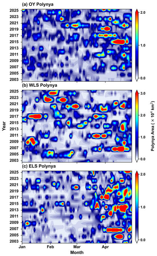
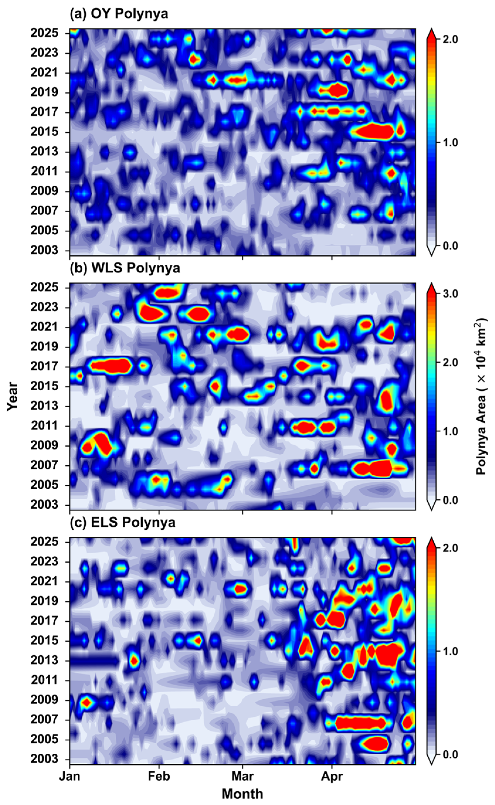
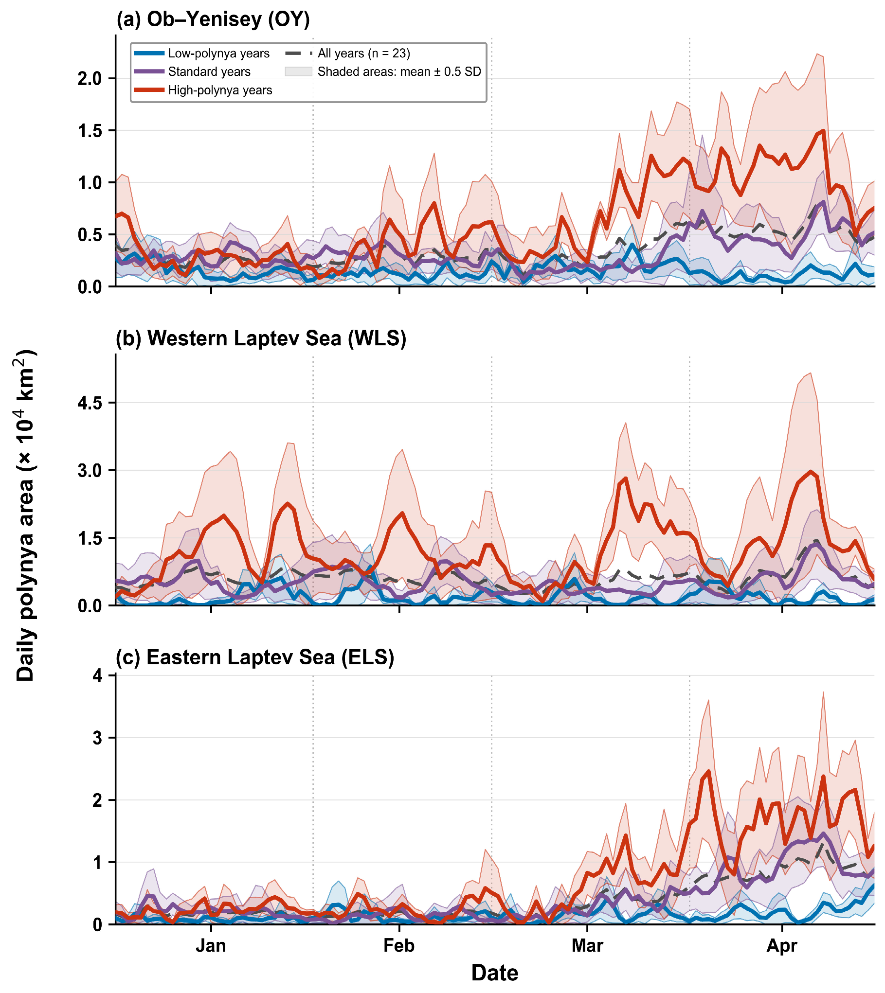
Figure 1, Figure 3, Figure 4 and Figure 5 show that the OY, WLS, and ELS systems cannot be treated as one uniform Kara–Laptev polynya regime. The OY is dominated by intermittent small-to-moderate activity with several late-season events; the WLS has the largest and most frequent episodic openings throughout January–April; and the ELS has the clearest recurrent late-March to April maximum. These contrasts persist across the spatial pattern, seasonal timing, and interannual record.
Figure 3.
Daily evolution of coastal-polynya area during January–April from 2003 to 2025: (a) OY, (b) WLS, and (c) ELS polynyas. The color scale indicates daily polynya area in units of 104 km2. Note that the upper color limits differ among panels to preserve regional detail.
Figure 4.
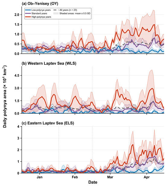
Region-specific, year-class-stratified seasonal evolution of daily coastal-polynya area in the OY, WLS, and ELS regions during January–April, 2003–2025. Years were classified independently within each region using January–April annual mean daily polynya areas and thresholds of the regional mean ± 0.75 SD. The resulting low-, standard-, and high-polynya groups contain n = 6, 11, and 6 years for the OY; n = 5, 13, and 5 years for the WLS; and n = 7, 11, and 5 years for the ELS, respectively. Colored lines show calendar-day group means, the matching semi-transparent shaded bands span the group mean ± 0.5 SD among years, and black dashed lines denote the all-year means (n = 23).
Figure 5.
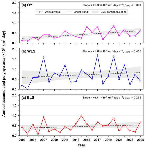
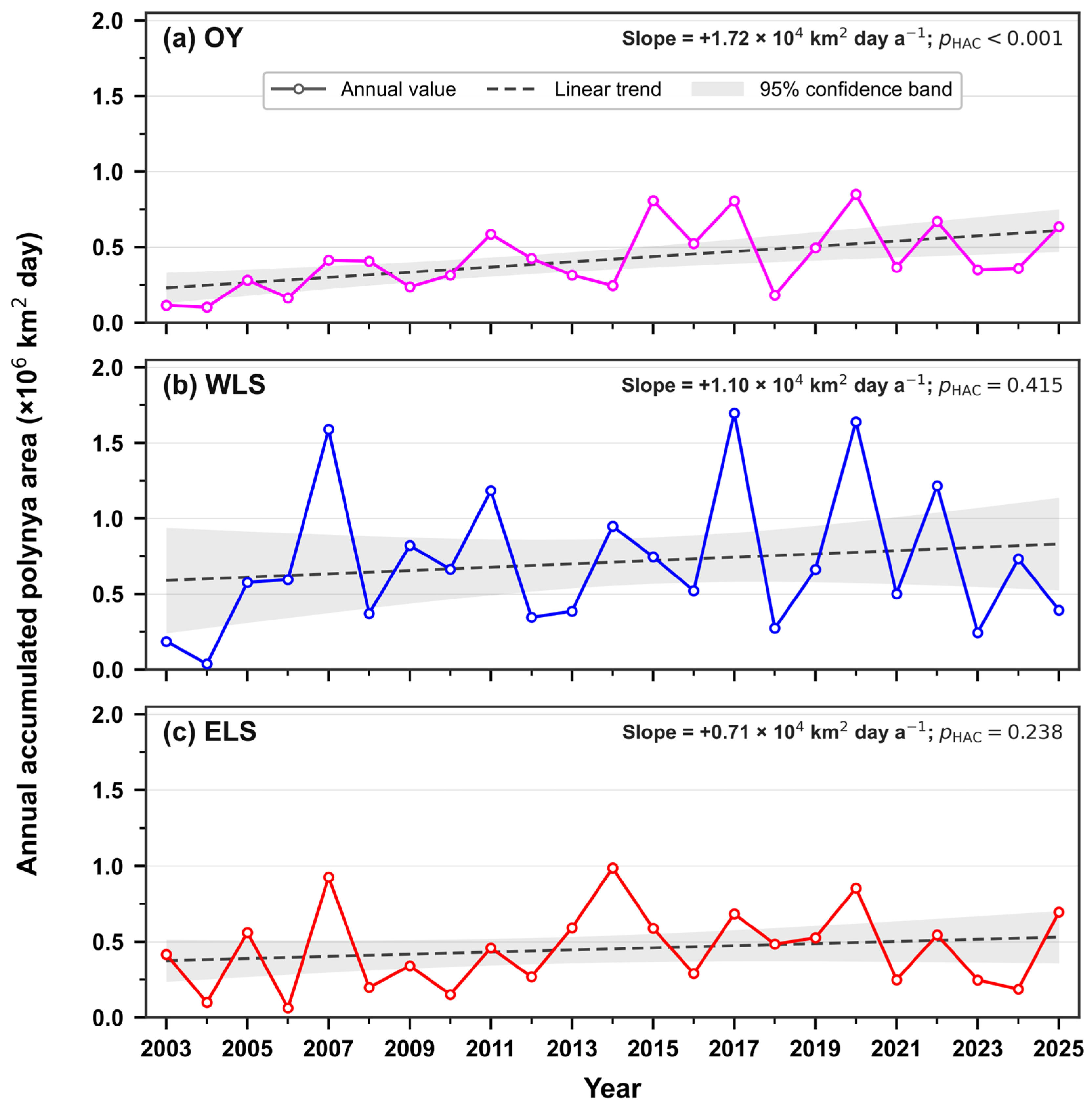
Interannual variability and linear trends in January–April accumulated coastal-polynya area in the OY, WLS, and ELS during 2003–2025: (a) OY, (b) WLS, and (c) ELS. Open circles connected by solid lines denote annual accumulated area in units of 106 km2 day. Dashed lines represent linear trends, and gray shading indicates the 95% confidence interval. Trend significance was evaluated using heteroskedasticity- and autocorrelation-consistent standard errors with a maximum lag of one year.
The year-class stratification in Figure 4 clarifies the timing of these distinct regimes. The OY and ELS separate most strongly in late March and April, whereas high-polynya WLS years can sustain event-scale activity across the full January–April season. The broad spread around several peaks shows that all three regional series remain strongly event-driven.
Event-size structure provides the same regional contrast: the WLS has the broadest distribution and the most frequent large-area conditions, whereas the OY is dominated by small events and the ELS is intermediate.
At the interannual scale (Figure 5), the OY shows the only statistically significant positive accumulated-area trend (+1.72 × 10⁴ km2 day a−1), but the increase is episodic rather than continuous. The five highest OY accumulated-area seasons occur in 2015, 2017, 2020, 2022, and 2025, while several intervening years remain lower. The fitted slope therefore reflects a cluster of high-area seasons from 2015 onward rather than a monotonic year-by-year increase. The WLS and ELS have positive but non-significant fitted slopes and are better characterized by recurrent high-area years than by persistent long-term increases.
Overall, all three fitted slopes are positive, but only the OY shows a statistically significant long-term increase. Across the complete 18-configuration detection-sensitivity matrix (Table S3; Figure S17), the WLS > ELS > OY ranking, the positive OY trend, and the signs of the environmental associations are retained; the OY trend is significant (p < 0.05) in 17 of 18 configurations and remains positive in the single exception (SIC 50%, Q90, no persistence screen; p = 0.084). The WLS and ELS instead display strong episodic variability, indicating that their accumulated areas are more strongly associated with year-specific events than with a steady multi-decadal trend.
3.2. Offshore Wind Provides the Short-Lag Opening Association
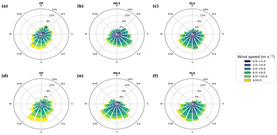
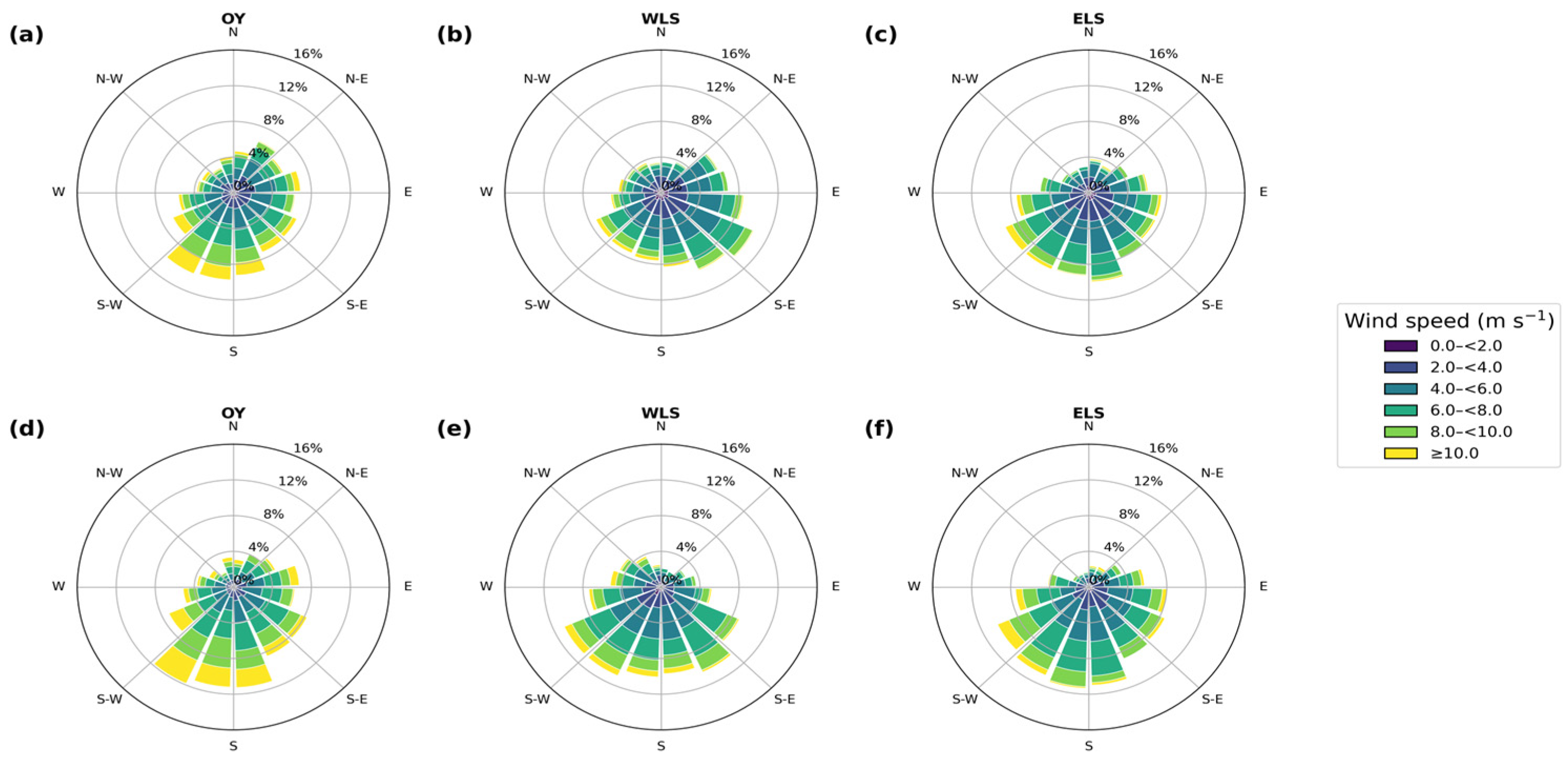
The normal-wind decomposition (Figure 6 and Table 3) shows that the wind direction physically favorable for ice divergence differs with regional geometry. Offshore-oriented winds are more frequent on polynya days in every region; the contrast is especially informative in the WLS, where favorable winds are less common overall but occur more often during polynya events. Thus, the same synoptic flow need not favor all three neighboring regions simultaneously.
Figure 6.
Wind-rose diagrams of January–April wind conditions during 2003–2025 for (a) the OY, (b) WLS, and (c) ELS. Panels (d–f) show wind conditions on polynya-occurrence days for the OY, WLS, and ELS, respectively. The legend uses consistent speed intervals (e.g., 0.0–<2.0 m s−1).
Table 3.
Orientation and January–April offshore-wind statistics for the OY, WLS, and ELS during 2003–2025.
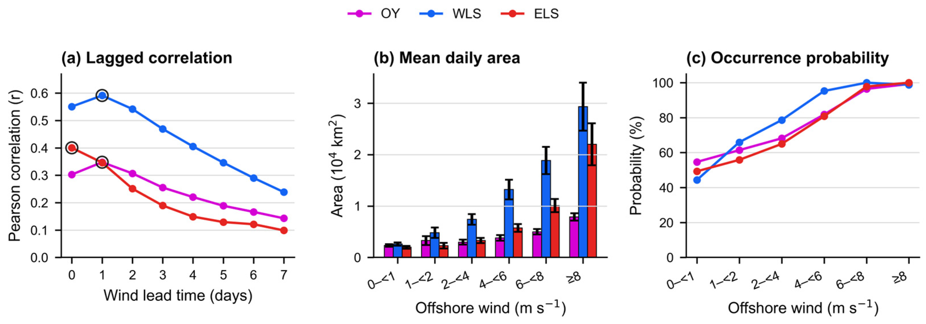
Offshore wind has the timing most consistent with immediate mechanical opening (Figure 7 and Table 4). Daily area is positively associated with offshore-wind speed in all regions; the strongest association occurs with a one-day wind lead in the OY and WLS and at zero lead in the ELS. The association weakens at longer leads, which is consistent with a rapid divergence response but does not by itself establish a unique causal pathway.
Figure 7.
Daily polynya area and offshore wind during January–April, 2003–2025, after excluding 29 February: (a) 0–7-day lead correlations (n = 2755 at zero lead; n is lead dependent); (b) mean daily area and (c) occurrence probability for same-day offshore-wind-speed bins of 0–<1, 1–<2, 2–<4, 4–<6, 6–<8, and ≥8 m s−1. Colors identify the region; bars show 95% confidence intervals.
Table 4.
Daily, lagged, and interannual Pearson correlations between polynya area and wind during January–April, 2003–2025. Daily and annual columns report Pearson r; “Maximum daily lead” gives the lead with the strongest correlation.
Across the daily, lagged, intensity-binned, and annual diagnostics, the local offshore component is more strongly associated with polynya area than the tangential component. Regional differences in magnitude and timing indicate that coastline orientation and background conditions are associated with the observed response.
3.3. Thermal and Ice-State Associations Vary by Region and Timescale
The timing diagnostics separate the wind association from the roles of thermal and ice variables. We treat NW as the variable most consistent with a short-lag opening mechanism, whereas T2M, SST, and SIT are evaluated as background conditions, synchronous state variables, or both. This distinction is essential because observational covariation cannot establish independent causal effects.
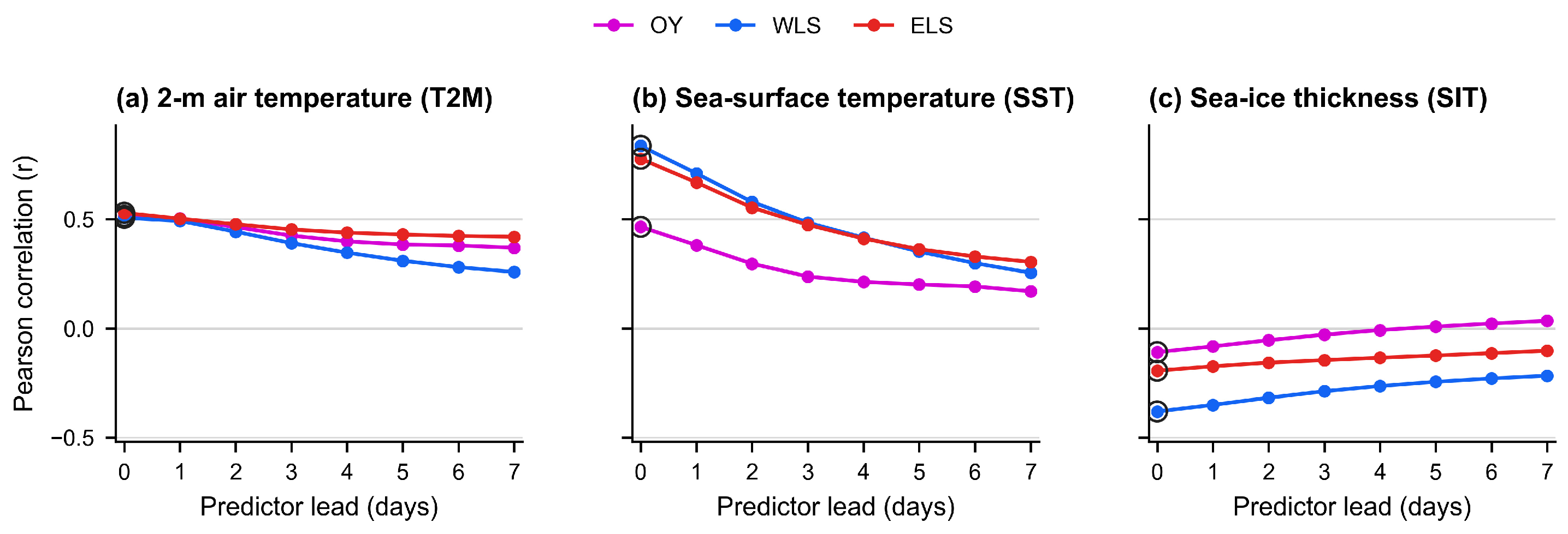
At the daily scale, T2M and SST are positively associated with polynya area and SIT is generally negatively associated (Figure 8). Their strongest direct relationships occur mainly at zero lead. The two-way-deseasonalized diagnostics in Table S6 therefore provide the principal basis for distinguishing antecedent timing from concurrent state dependence.
Figure 8.
Lead-time Pearson correlations of daily polynya area with (a) T2M, (b) SST, and (c) SIT in January–April, 2003–2025. Predictors lead by k days (t − k); pairs were calendar-date matched within years. Outlined points mark maximum |r|. At zero lead, n = 2755 for T2M and SIT and n = 2635 for SST (unavailable in 2012).
SST has the strongest same-day partial association in the WLS and ELS, while SIT also peaks mainly at zero lead. SST and SIT are therefore interpreted primarily as synchronous ice–ocean and sea-ice state indicators, with possible background components, rather than as demonstrated immediate forcings. In particular, high same-day SST may reflect pre-existing thermal conditions, open-water exposure after polynya opening, and/or the retrieval signature of open water or thin ice.
Calendar-day climatologies (Figure S9) and the year-clustered, two-way-deseasonalized diagnostics (Table S6; Figure S10) retain the principal signs and regional contrasts after reducing shared seasonality and year-to-year offsets. These results support interpretation based on the observed timing while avoiding causal claims from raw correlations.
At the annual scale, warmer T2M and thinner SIT are statistically associated with greater polynya activity across the three regions, while the SST association is strongest in the WLS. The complete coefficient set and the annual visual diagnostics are reported in Table S7 and Figures S11 and S12 rather than repeated in the main text.
The timing evidence identifies NW as the only variable with a clear short-lag peak in the OY and WLS, whereas T2M, SST, and SIT mainly characterize antecedent background conditions and/or the synchronous state of the ice–ocean system. Accordingly, the multifactor results below are interpreted jointly with the lead-time diagnostics.
The multifactor models provide a compact synthesis of the covarying wind, thermal, and ice variables. Daily models use two-way-deseasonalized anomalies, so they describe within-season covariability after removal of regional calendar-day climatology and within-year offsets; annual models describe accumulated-area associations. In both cases, hierarchical partitioning (HP) is interpreted as relative explanatory allocation, not as independent causal attribution.
Collinearity is weak in the daily anomaly models (maximum VIF < 1.5) but material at the annual scale, especially for WLS NW (VIF = 8.84; tolerance = 0.11). Figure S13 visualizes the pairwise predictor covariance, and the complete VIF and tolerance diagnostics are provided in Table S5 and Figure S14. The zero-order, partial-correlation, and standardized-coefficient diagnostics in Tables S8 and S9 are therefore integral to the HP interpretation.
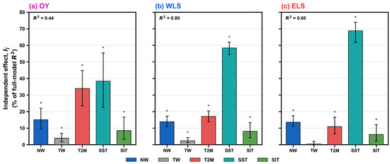
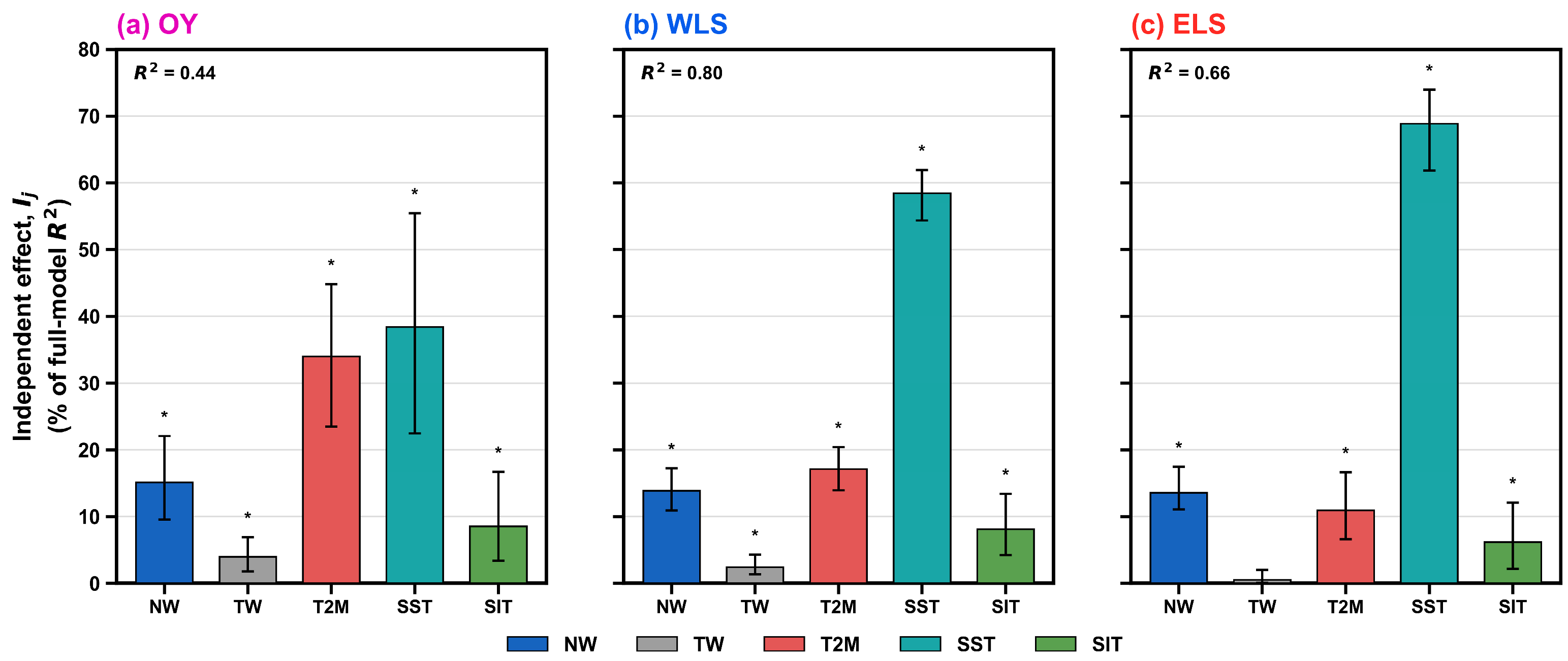
The daily models explain 44%, 80%, and 66% of deseasonalized anomaly variance in the OY, WLS, and ELS, respectively (Figure 9). HP assigns the largest daily allocation to SST in the WLS and ELS, but SST’s predominantly zero-lead timing indicates a concurrent state association rather than an antecedent oceanic control. In the OY, the allocation is more evenly distributed among the thermal variables.
Figure 9.
Hierarchical partitioning of daily anomaly polynya-area models for the OY, WLS, and ELS: (a) OY, (b) WLS, and (c) ELS. Bars show average incremental R2 allocations as percentages of the full-model R2, not independent causal effects. Error bars indicate year-block bootstrap 95% confidence intervals; asterisks denote p < 0.05 from permutation tests.
At the annual scale, the allocations are more region dependent (Table 5): the OY is most strongly associated with T2M and NW, whereas the WLS and ELS show larger combined allocations to SST, SIT, and NW. The annual WLS pattern is interpreted cautiously because of collinearity; the allocation does not identify a single independent driver.
Table 5.
Model fit and predictor-specific relative explanatory allocations from hierarchical partitioning.
Taken together, these diagnostics show that NW has the clearest short-lag association with polynya opening, whereas the thermal and ice variables characterize regional conditions. HP allocations are interpreted alongside timing and collinearity and do not represent independent causal effects.
4. Discussion
First, the three adjacent polynya systems should not be treated as a uniform Kara–Laptev regime. Their different coastline orientations, landfast-ice settings, and seasonal timing help explain why comparable synoptic conditions are associated with different responses.
Second, offshore wind has the timing most consistent with rapid opening. The one-day lead in the OY and WLS and the same-day peak in the ELS are consistent with mechanical divergence, but these regional contrasts do not identify a single causal pathway.
Third, geometry together with thermal and ice-state conditions is associated with the magnitude and persistence of polynya activity. T2M and SIT describe background thermodynamic and sea-ice conditions, whereas the predominantly synchronous SST association may also reflect open-water exposure or thin-ice retrieval. River discharge can affect nearshore salinity, stratification, and ice–ocean interaction [45,46,47], but it remains unmodeled background context (Figure S15), not an immediate trigger or a primary explanatory variable.
These interpretations remain bounded by the 6.25 km passive-microwave SIC record, the spatial-reference role of the 1 km merged SIC product (Table S2), missing SST in 2012, reanalysis-based SIT, and the observational design. Exploratory AO/ENSO and spectral comparisons are retained in Table S10 and Figure S16 of the Supplementary Materials as context, not as a fourth mechanism. Accordingly, correlations, coefficients, and HP allocations are interpreted as statistical associations.
5. Conclusions
This study compared January–April coastal-polynya variability in the Kara–Laptev Seas from 2003 to 2025 using one consistent framework for the OY, WLS, and ELS. The conclusions are organized around three findings.
First, adjacent Kara–Laptev polynyas are not one uniform system. The OY is concentrated near the Ob–Yenisey River mouths and shows the only significant accumulated-area increase, with high-area seasons clustered from 2015 onward rather than rising year by year. The WLS has the broadest event-size distribution and the most frequent large-area days, whereas the ELS is most concentrated in late March and April. The WLS > ELS > OY ranking, the positive OY trend, and the signs of the environmental associations are retained across all 18 configurations of the detection-sensitivity matrix, with the OY trend significant in 17 of 18 configurations.
Second, NW has the timing most consistent with immediate mechanical opening. Daily area is positively associated with offshore wind in all regions; the strongest NW relationship occurs when wind leads by one day in the OY and WLS and on the same day in the ELS. This short timing, together with local coastline orientation, is consistent with rapid wind-driven divergence, but these observational results do not establish a unique causal mechanism.
Third, regional geometry and thermal and sea-ice conditions are associated with the magnitude and persistence of polynya activity. T2M, SST, and SIT show substantial daily and annual statistical associations, but the timing diagnostics indicate that SST is predominantly synchronous. HP therefore provides relative explanatory allocation among covarying predictors, not independent causal attribution; this distinction is especially important for the collinear annual WLS model.
Overall, offshore wind is associated with rapid opening, whereas regional geometry, temperature, and ice thickness are associated with magnitude and persistence. These findings distinguish the OY, WLS, and ELS without implying causal effects from observational statistics.
Supplementary Materials
The following supporting information can be downloaded at: https://www.mdpi.com/article/10.3390/rs18172914/s1, Figure S1: SSMIS consistency assessment; Figure S2: Daily surface-temperature and T2M climatology; Figure S3: Spatial SIC-threshold sensitivity; Figure S4: Accumulated-area SIC-threshold sensitivity; Figure S5: AMSR2 comparison with a 1 km merged SIC reference; Figure S6: Monthly SIC and SIT climatology; Figure S7: Temporal-persistence screening; Figure S8: Region-specific year classification; Figure S9: Daily climatologies of polynya area, T2M, SST, and SIT; Figure S10: Deseasonalized lag correlations; Figure S11: Annual accumulated-area relationships with background factors; Figure S12: Annual occurrence-frequency relationships with background factors; Figure S13: Annual predictor-correlation matrices; Figure S14: Daily and annual VIF diagnostics; Figure S15: River discharge; Figure S16: Exploratory AO/ENSO context; Figure S17: Detection-sensitivity matrix summary; Table S1: Datasets and preprocessing; Table S2: 1 km reference comparisons; Table S3: Complete 3 × 3 × 2 detection-sensitivity matrix; Table S4: Grid-cell low-SIC duration statistics; Table S5: Full collinearity diagnostics; Table S6: Time-role diagnostics; Table S7: Annual background correlations; Table S8: Daily-anomaly directional diagnostics; Table S9: Annual directional diagnostics; Table S10: Exploratory climate-mode and spectral context.
Author Contributions
Conceptualization and methodology, X.B. and Z.D.; writing—original draft preparation, Z.D. and M.H.; writing—review and editing, Z.D., M.H., X.J. and X.B.; visualization, Z.D. and X.J.; supervision, X.B.; funding acquisition, X.B. and M.H. All authors have read and agreed to the published version of the manuscript.
Funding
This research was funded by the National Natural Science Foundation of China (grant Nos. 42276254 and 42375016), the National Key Research and Development Program of China (grant No. 2017YFA0604602).
Data Availability Statement
The datasets used in this study are publicly available. Sea-ice concentration data were obtained from the University of Bremen: https://data.seaice.uni-bremen.de/ (accessed on 27 August 2026). ERA5 reanalysis data, including 10 m wind and 2 m air temperature, are available from the Copernicus Climate Data Store: https://cds.climate.copernicus.eu/datasets (accessed on 27 August 2026). AMSR-MPR data were obtained from the University of Bremen Multi-Parameter product: https://data.seaice.uni-bremen.de/MultiParameter/ (accessed on 27 August 2026). Sea-ice thickness data were obtained from the Copernicus Marine Service Arctic Ocean Physics Reanalysis/TOPAZ4b product: https://data.marine.copernicus.eu/product/ARCTIC_MULTIYEAR_PHY_002_003/description (accessed on 27 August 2026). The Arctic Oscillation and Niño 3.4 indices are available from NOAA: https://www.cpc.ncep.noaa.gov/data/indices/ (accessed on 27 August 2026). River discharge data were obtained from the Arctic Great Rivers Observatory: https://arcticgreatrivers.org/data/ (accessed on 27 August 2026). Selected processing and analysis scripts are available at https://github.com/dzq9911-create/Spatiotemporal-Characteristics-and-Drivers-of-Coastal-Polynyas-in-the-Kara-and-Laptev-Seas (accessed on 27 August 2026). The no-leap recalculation files and derived outputs supporting this revision are available from the corresponding author upon reasonable request.
Acknowledgments
We acknowledge the data providers for making their products publicly available, including the University of Bremen sea-ice concentration dataset, the Copernicus Climate Data Store, NOAA, and the Arctic Great Rivers Observatory river discharge records. The authors have reviewed and edited the output and take full responsibility for the content of this publication.
Conflicts of Interest
The authors declare no conflicts of interest.
Abbreviations
The following abbreviations are used in this manuscript:
| OY | Ob–Yenisey |
| WLS | Western Laptev Sea |
| ELS | Eastern Laptev Sea |
| SIC | Sea ice concentration |
| SIT | Sea-ice thickness |
| T2M | 2 m air temperature |
| SST | Sea-surface temperature |
| TSA | Surface temperature |
| NW | Normal wind |
| TW | Tangential wind |
| AO | Arctic Oscillation |
| ENSO | El Niño–Southern Oscillation |
| Niño 3.4 | Niño 3.4 index |
| HP | Hierarchical partitioning |
| VIF | Variance inflation factor |
| PSD | Power spectral density |
| SD | Standard deviation |
| Q75 | 75th percentile |
| Q95 | 95th percentile |
| ERA5 | Fifth-generation ECMWF atmospheric reanalysis |
| NOAA | The National Oceanic and Atmospheric Administration |
| AMSR | The Advanced Microwave Scanning Radiometer |
| SSMIS | The Special Sensor Microwave Imager/Sounder |
| MPR | Multi-parameter Retrieval |
| IUP | Institute of Environmental Physics |
| ECMWF | European Centre for Medium-Range Weather Forecasts |
| NERSC | Nansen Environmental and Remote Sensing Center |
| TOPAZ4b | Arctic Ocean Physics Reanalysis product |
| ArcticGRO | Arctic Great Rivers Observatory |
References
- Comiso, J.C. Abrupt decline in the Arctic winter sea ice cover. Geophys. Res. Lett. 2006, 33, L18504. [Google Scholar] [CrossRef] [Scilit]
- Smith, S.D.; Muench, R.D.; Pease, C.H. Polynyas and leads: An overview of physical processes and environment. J. Geophys. Res. Oceans 1990, 95, 9461–9479. [Google Scholar] [CrossRef] [Scilit]
- Morales Maqueda, M.A.; Willmott, A.J.; Biggs, N.R.T. Polynya Dynamics: A Review of Observations and Modeling. Rev. Geophys. 2004, 42, RG1004. [Google Scholar] [CrossRef] [Scilit]
- Tamura, T.; Ohshima, K.I. Mapping of sea ice production in the Arctic coastal polynyas. J. Geophys. Res. Oceans 2011, 116, C07030. [Google Scholar] [CrossRef] [Scilit]
- Pease, C.H. The size of wind-driven coastal polynyas. J. Geophys. Res. Oceans 1987, 92, 7049–7059. [Google Scholar] [CrossRef] [Scilit]
- Morales Maqueda, M.A.; Willmott, A.J.; Walkington, I.A. The opening of wind-driven polynyas. J. Fluid Mech. 2014, 746, 236–272. [Google Scholar] [CrossRef] [Scilit][Green Version]
- Chao, S.Y. Ocean feedback to wind-driven coastal polynyas. J. Geophys. Res. Oceans 1999, 104, 18073–18085. [Google Scholar] [CrossRef] [Scilit]
- Dmitrenko, I.A.; Wegner, C.; Kassens, H.; Kirillov, S.A.; Krumpen, T.; Heinemann, G.; Helbig, A.; Schröder, D.; Hölemann, J.A.; Klagge, T.; et al. Observations of supercooling and frazil ice formation in the Laptev Sea coastal polynya. J. Geophys. Res. Oceans 2010, 115, C05015. [Google Scholar] [CrossRef] [Scilit]
- Dmitrenko, I.A.; Kirillov, S.A.; Bloshkina, E.; Lenn, Y.D. Tide-induced vertical mixing in the Laptev Sea coastal polynya. J. Geophys. Res. Oceans 2012, 117, C00G14. [Google Scholar] [CrossRef] [Scilit]
- Kirillov, S.A.; Dmitrenko, I.A.; Hölemann, J.A.; Kassens, H.; Bloshkina, E. The penetrative mixing in the Laptev Sea coastal polynya pycnocline layer. Cont. Shelf Res. 2013, 63, 34–42. [Google Scholar] [CrossRef] [Scilit]
- Willmes, S.; Adams, S.; Schröder, D.; Heinemann, G. Spatio-temporal variability of polynya dynamics and ice production in the Laptev Sea between the winters of 1979/80 and 2007/08. Polar Res. 2011, 30, 5971. [Google Scholar] [CrossRef] [Scilit]
- Bauer, M.; Schröder, D.; Heinemann, G.; Willmes, S.; Ebner, L. Quantifying polynya ice production in the Laptev Sea with the COSMO model. Polar Res. 2013, 32, 20922. [Google Scholar] [CrossRef] [Scilit]
- Eicken, H.; Dmitrenko, I.; Tyshko, K.; Darovskikh, A.; Dierking, W.; Blahak, U.; Groves, J.; Kassens, H. Zonation of the Laptev Sea landfast ice cover and its importance in a frozen estuary. Glob. Planet. Change 2005, 48, 55–83. [Google Scholar] [CrossRef] [Scilit]
- Rabenstein, L.; Krumpen, T.; Hendricks, S.; Koeberle, C.; Haas, C.; Hoelemann, J.A. A combined approach of remote sensing and airborne electromagnetics to determine the volume of polynya sea ice in the Laptev Sea. Cryosphere 2013, 7, 947–959. [Google Scholar] [CrossRef] [Scilit]
- Winsor, P.; Björk, G. Polynya activity in the Arctic Ocean from 1958 to 1997. J. Geophys. Res. Oceans 2000, 105, 8789–8803. [Google Scholar] [CrossRef] [Scilit]
- Stringer, W.J.; Groves, J.E. Location and Areal Extent of Polynyas in the Bering and Chukchi Seas. Arctic 1991, 44, 164–171. [Google Scholar] [CrossRef] [Scilit]
- Preußer, A.; Heinemann, G.; Willmes, S.; Paul, S. Multi-Decadal Variability of Polynya Characteristics and Ice Production in the North Water Polynya by Means of Passive Microwave and Thermal Infrared Satellite Imagery. Remote Sens. 2015, 7, 15844–15867. [Google Scholar] [CrossRef] [Scilit]
- Vincent, R.F. An Assessment of the Lancaster Sound Polynya Using Satellite Data 1979 to 2022. Remote Sens. 2023, 15, 954. [Google Scholar] [CrossRef] [Scilit]
- Bradtke, K.; Brodziński, W.; Herman, A. Signatures of Breaking Waves in a Coastal Polynya Covered with Frazil Ice: A High-Resolution Satellite Image Case Study of Terra Nova Bay Polynya. Remote Sens. 2025, 17, 3198. [Google Scholar] [CrossRef] [Scilit]
- University of Bremen. AMSR-E/AMSR2 Sea Ice Concentration Data. Available online: https://data.seaice.uni-bremen.de/ (accessed on 27 August 2026).
- Kaleschke, L.; Lüpkes, C.; Vihma, T.; Haarpaintner, J.; Bochert, A.; Hartmann, J.; Heygster, G. SSM/I Sea Ice Remote Sensing for Mesoscale Ocean-Atmosphere Interaction Analysis. Can. J. Remote Sens. 2001, 27, 526–537. [Google Scholar] [CrossRef] [Scilit]
- Kern, S.; Kaleschke, L.; Clausi, D.A. A Comparison of Two 85-GHz SSM/I Ice Concentration Algorithms with AVHRR and ERS-2 SAR Imagery. IEEE Trans. Geosci. Remote Sens. 2003, 41, 2294–2306. [Google Scholar] [CrossRef] [Scilit]
- Spreen, G.; Kaleschke, L.; Heygster, G. Sea ice remote sensing using AMSR-E 89-GHz channels. J. Geophys. Res. Oceans 2008, 113, C02S03. [Google Scholar] [CrossRef] [Scilit]
- Pang, X.; Pu, J.; Zhao, X.; Ji, Q.; Qu, M.; Cheng, Z. Comparison between AMSR2 Sea Ice Concentration Products and Pseudo-Ship Observations of the Arctic and Antarctic Sea Ice Edge on Cloud-Free Days. Remote Sens. 2018, 10, 317. [Google Scholar] [CrossRef] [Scilit]
- University of Bremen. Multi-Parameter Retrieval Product. Available online: https://data.seaice.uni-bremen.de/MultiParameter/ (accessed on 27 August 2026).
- Copernicus Marine Service. Arctic Ocean Physics Reanalysis. Available online: https://data.marine.copernicus.eu/product/ARCTIC_MULTIYEAR_PHY_002_003/description (accessed on 27 August 2026).
- Sakov, P.; Counillon, F.; Bertino, L.; Lisæter, K.A.; Oke, P.R.; Korablev, A. TOPAZ4: An ocean-sea ice data assimilation system for the North Atlantic and Arctic. Ocean Sci. 2012, 8, 633–656. [Google Scholar] [CrossRef] [Scilit]
- Kacimi, S.; Kwok, R. Two Decades of Arctic Sea-Ice Thickness from Satellite Altimeters: Retrieval Approaches and Record of Changes (2003–2023). Remote Sens. 2024, 16, 2983. [Google Scholar] [CrossRef] [Scilit]
- Stroeve, J.; Barrett, A.; Serreze, M.; Schweiger, A. Using records from submarine, aircraft and satellites to evaluate climate model simulations of Arctic sea ice thickness. Cryosphere 2014, 8, 1839–1854. [Google Scholar] [CrossRef] [Scilit]
- Hersbach, H.; Bell, B.; Berrisford, P.; Hirahara, S.; Horányi, A.; Muñoz-Sabater, J.; Nicolas, J.; Peubey, C.; Radu, R.; Schepers, D.; et al. The ERA5 global reanalysis. Q. J. R. Meteorol. Soc. 2020, 146, 1999–2049. [Google Scholar] [CrossRef] [Scilit]
- NOAA Physical Sciences Laboratory. Arctic Oscillation Index. Available online: https://psl.noaa.gov/data/timeseries/month/AO/ (accessed on 27 August 2026).
- NOAA Climate Prediction Center. Monthly Atmospheric and Sea-Surface Temperature Indices. Available online: https://www.cpc.ncep.noaa.gov/data/indices/ (accessed on 27 August 2026).
- Thompson, D.W.J.; Wallace, J.M. The Arctic oscillation signature in the wintertime geopotential height and temperature fields. Geophys. Res. Lett. 1998, 25, 1297–1300. [Google Scholar] [CrossRef] [Scilit]
- Trenberth, K.E. The Definition of El Niño. Bull. Am. Meteorol. Soc. 1997, 78, 2771–2777. [Google Scholar] [CrossRef] [Scilit]
- Arctic Great Rivers Observatory. Discharge Data. Available online: https://arcticgreatrivers.org/data/ (accessed on 27 August 2026).
- Markus, T.; Burns, B.A. A method to estimate subpixel-scale coastal polynyas with satellite passive microwave data. J. Geophys. Res. Oceans 1995, 100, 4473–4487. [Google Scholar] [CrossRef] [Scilit]
- Martin, S.; Drucker, R.; Kwok, R.; Holt, B. Estimation of the thin ice thickness and heat flux for the Chukchi Sea Alaskan coast polynya from Special Sensor Microwave/Imager data, 1990–2001. J. Geophys. Res. Oceans 2004, 109, C10012. [Google Scholar] [CrossRef] [Scilit]
- Mäkynen, M.; Similä, M. Arctic Thin Ice Detection Using AMSR2 and FY-3C MWRI Radiometer Data. Remote Sens. 2024, 16, 1600. [Google Scholar] [CrossRef] [Scilit]
- Dormann, C.F.; Elith, J.; Bacher, S.; Buchmann, C.; Carl, G.; Carré, G.; Marquéz, J.R.G.; Gruber, B.; Lafourcade, B.; Leitão, P.J.; et al. Collinearity: A review of methods to deal with it and a simulation study evaluating their performance. Ecography 2013, 36, 27–46. [Google Scholar] [CrossRef] [Scilit]
- O’Brien, R.M. A Caution Regarding Rules of Thumb for Variance Inflation Factors. Qual. Quant. 2007, 41, 673–690. [Google Scholar] [CrossRef] [Scilit]
- Chevan, A.; Sutherland, M. Hierarchical Partitioning. Am. Stat. 1991, 45, 90–96. [Google Scholar] [CrossRef] [Scilit]
- Grömping, U. Estimators of Relative Importance in Linear Regression Based on Variance Decomposition. Am. Stat. 2007, 61, 139–147. [Google Scholar] [CrossRef] [Scilit]
- Giam, X.; Olden, J.D. Quantifying variable importance in a multimodel inference framework. Methods Ecol. Evol. 2016, 7, 388–397. [Google Scholar] [CrossRef] [Scilit]
- Efron, B. Bootstrap Methods: Another Look at the Jackknife. Ann. Stat. 1979, 7, 1–26. [Google Scholar] [CrossRef] [Scilit]
- Peterson, B.J.; Holmes, R.M.; McClelland, J.W.; Vörösmarty, C.J.; Lammers, R.B.; Shiklomanov, A.I.; Shiklomanov, I.A.; Rahmstorf, S. Increasing River Discharge to the Arctic Ocean. Science 2002, 298, 2171–2173. [Google Scholar] [CrossRef] [Scilit]
- McClelland, J.W.; Déry, S.J.; Peterson, B.J.; Holmes, R.M.; Wood, E.F. A pan-arctic evaluation of changes in river discharge during the latter half of the 20th century. Geophys. Res. Lett. 2006, 33, L06715. [Google Scholar] [CrossRef] [Scilit]
- McClelland, J.W.; Holmes, R.M.; Peterson, B.J.; Stieglitz, M. Increasing river discharge in the Eurasian Arctic: Consideration of dams, permafrost thaw, and fires as potential agents of change. J. Geophys. Res. Atmos. 2004, 109, D18102. [Google Scholar] [CrossRef] [Scilit]

Disclaimer/Publisher’s Note: The statements, opinions and data contained in all publications are solely those of the individual author(s) and contributor(s) and not of MDPI and/or the editor(s). MDPI and/or the editor(s) disclaim responsibility for any injury to people or property resulting from any ideas, methods, instructions or products referred to in the content. |
© 2026 by the authors. Licensee MDPI, Basel, Switzerland. This article is an open access article distributed under the terms and conditions of the Creative Commons Attribution (CC BY) license.