


Highlights
What are the main findings?
- GRACE TWS can be reliably gap-filled and downscaled using a bias-aware Random Forest framework.
- The mass-conserving correction reduces spatial bias while preserving the original GRACE water-storage signal.
What is the implication of the main finding?
- The method supports water-resource assessment in data-scarce and conflict-affected transboundary basins.
Abstract
GRACE and GRACE-FO satellite gravimetry provide unique observations of terrestrial water storage (TWS), but their coarse effective resolution and intermittent temporal gaps limit water-resource applications at subregional and basin scales. This study presents a framework to temporally reconstruct and spatially downscale GRACE TWS anomalies for the transboundary Bug River Basin (Poland–Ukraine–Belarus), a region where in situ monitoring is limited and further disrupted by the 2022 war in Ukraine. First, missing monthly GRACE TWS anomalies (2002–2024) are imputed using a Random Forest model driven only by lagged GRACE values (1–3 months) and seasonal timing, thereby avoiding potential information leakage. Second, the continuous GRACE signal is downscaled to 0.1° using an independent set of hydroclimatic predictors with lagged and rolling features, together with elevation, land type and lithology. Model performance is evaluated under strict spatiotemporal holdouts and cross-validation. The key methodological advance is a bias-aware, block-wise mass-conserving correction that reconciles downscaled fields with the original GRACE water mass at coarse resolution. After downscaling to 0.1°, systematic residual biases between aggregated high-resolution estimates and GRACE observations are quantified monthly and redistributed within spatial blocks using river-runoff-based weights. This procedure enforces exact mass closure while preserving physically meaningful sub-grid variability.
1. Introduction
The Gravity Recovery and Climate Experiment (GRACE) and its successor GRACE Follow-On (GRACE-FO) have transformed terrestrial water monitoring by measuring temporal variations in Earth’s gravitational field rather than relying on electromagnetic remote sensing [1,2]. This capability is based on the fundamental relationship between the gravitational field and mass distribution. Temporal changes in gravity reflect mass redistribution within the Earth system, and after accounting for atmospheric, oceanic, and solid-Earth contributions, these signals can be interpreted primarily as changes in terrestrial water storage (TWS). This capability has enabled direct estimation of water storage variations, including groundwater, soil moisture, surface water, snow, and ice, representing a breakthrough in large-scale hydrological monitoring [3].
GRACE observations of TWS have proven particularly valuable for detecting long-term trends in water resources that are difficult to observe using conventional in situ measurements. At continental and subcontinental scales, GRACE has revealed significant declines in water storage associated with climate change and unsustainable water use, including in northern India [4,5,6,7], northern China [8,9,10], and the Middle East [11,12]. Beyond trend detection, GRACE data have increasingly been used to constrain and evaluate hydrological and climate models, reducing model uncertainty and improving simulations of water cycle components [13,14,15].
The utility of GRACE is particularly pronounced in regions where ground-based hydrological monitoring is sparse, disrupted, or inaccessible. The transboundary Bug River Basin (BRB), spanning Poland, Ukraine, and Belarus, exemplifies these challenges. The 2022 Russian invasion of Ukraine has further destabilized regional water monitoring, with damaged infrastructure, disrupted gauge networks, and restricted data sharing. Independent of conflict impacts, the BRB has experienced a documented decline in surface water resources exceeding 20% over the past two decades, attributed largely to regional climate warming [16]. GRACE-based analyses further indicate a sustained decline in TWS in the basin, exceeding 9 mm yr−1 over the past decade [17], with climate projections suggesting continued warming throughout the 21st century [18].
Despite its strengths, a key limitation of GRACE is its coarse effective spatial resolution. GRACE solutions based on spherical harmonic coefficients have an effective spatial resolution of approximately 300–400 km, resulting from spherical harmonic truncation and the spatial filtering required to suppress the characteristic north–south striping noise [19]. More recent mascon solutions, using strong spatial regularization and a priori constraints, avoid the need for post-processing filtering and improve spatial localization, achieving effective resolutions on the order of 200–300 km [20]. However, this resolution remains insufficient for basin-scale water management, where decision-relevant processes typically occur at spatial scales of 10–50 km. To address this limitation, numerous downscaling approaches have emerged over the past 15 years. These approaches broadly fall into three categories: (i) statistical methods, such as regression-based scaling with higher-resolution hydroclimatic variables [21,22]; (ii) data assimilation techniques that integrate GRACE observations into land surface models [23,24,25,26,27]; and (iii) machine learning (ML) methods—particularly Random Forests (RF) and neural networks—that exploit nonlinear relationships between GRACE-derived TWS and high-resolution hydro-climatic predictors [28,29,30]. Deep learning methods have also been applied to TWS gap imputation, including Bayesian convolutional neural networks [31] and transformers [32], as well as for downscaling using generative adversarial networks [33], Gated Recurrent Units [34], and Long Short-Term Memory (LSTM) recurrent neural networks [35].
While statistical approaches are computationally efficient, they may oversimplify spatial heterogeneity of TWS. Data assimilation improves physical consistency by integrating GRACE into land surface models but remains sensitive to model structure and parameterization. ML methods offer flexibility in capturing complex relationships, though their performance depends critically on predictor selection, bias handling, and validation strategy. Another challenge in utilizing GRACE data for hydrological applications is the nearly one-year gap between the end of the GRACE mission and the beginning of GRACE-FO operations, as well as additional gaps of up to several months within both GRACE and GRACE-FO time series. Continuous TWS records, which are essential for water resources monitoring and management, are currently unavailable and thus require gap filling using statistical methods [36,37,38], ML techniques [39,40,41] or the integration of complementary data from other sources [42,43,44].
Building on prior work in the BRB [17], this study advances GRACE-based TWS downscaling by systematically addressing predictor-induced bias and spatial heterogeneity in a transboundary, data-limited, and conflict-affected region. Using an RF framework and a suite of hydro-climatic (precipitation, evapotranspiration, river runoff, and soil moisture storage) and physiographic (elevation, lithology, land cover) predictors, we downscale GRACE TWS anomalies from their native coarse resolution to a finer spatial grid suitable for basin-scale analysis. The resulting product enables improved characterization of sub-basin water storage dynamics while maintaining consistency with original GRACE observations.
Previous studies in the BRB have demonstrated the potential of GRACE observations for analyzing basin-scale TWS changes and integrating satellite-derived TWS with water-balance components (e.g., [17,44]). These studies were conducted at the native spatial resolution of the GRACE products and did not address spatial downscaling. Missing GRACE observations, including the GRACE–GRACE-FO data gap, were reconstructed using AutoRegressive Integrated Moving Average (ARIMA) models based solely on the temporal evolution of GRACE-derived TWS. More recently, RF-based spatial downscaling of GRACE-derived TWS was introduced for the BRB using meteorological predictors, while missing observations were still reconstructed using ARIMA [45]. Building upon these studies, the present work introduces a unified ML framework that (i) reconstructs missing GRACE observations using ML and month encoding, (ii) performs TWS downscaling using an expanded set of predictors, including not only hydrometeorological variables but also land surface characteristics (e.g., land surface temperature, elevation, lithology, and land cover), and (iii) introduces a novel bias-aware mass-conserving correction to preserve consistency with the original GRACE observations.
This study was conducted as part of the GRANDE-U (Groundwater Resilience Assessment through Integrated Data Exploration for Ukraine) project, whose mission is to advance transboundary groundwater resilience assessment by integrating physics-based and ML models with remote sensing data. With transboundary aquifers providing a significant share of drinking and irrigation water worldwide, effective management requires a robust foundation built on shared observations and models, coordinated assessments, and aligned perceptions of groundwater recharge and use. The GRANDE-U project addresses these challenges through an organizational and technological framework uniting researchers from six countries—the U.S., Ukraine, Poland, Latvia, Lithuania, and Estonia—to share best practices for resilience assessment in areas with disjointed data collection, uneven monitoring networks, and limited international coordination.
The specific contributions of this study are threefold: (i) to evaluate bias-aware ML downscaling of GRACE TWS in a climatically and politically complex transboundary basin; (ii) to quantify the consistency and uncertainty of downscaled TWS estimates relative to original GRACE signals and independent sources of TWS information; and (iii) to demonstrate the applicability of the approach for water resource assessment in regions where conventional monitoring is limited or disrupted.
2. Environmental Setting
The BRB represents an area of recognized importance for regional water resource management in Central and Eastern Europe. Previous hydrogeological syntheses indicate the presence of a large groundwater system that contributes substantially to drinking water supply in parts of Poland and Ukraine. In the literature, this system has been classified as a subregional groundwater reservoir with relatively large estimated resources, and it is commonly discussed in the context of strategic freshwater reserves [46].
The BRB covers an area of approximately 40,000 km2. The Bug River has a total length of 772 km, with the Krzna, Mścisławka, and Włodawka rivers among its major tributaries. The basin exhibits pronounced physiographic heterogeneity. Lowland landscapes (the East Baltic–Belarusian Lowlands) dominate roughly three quarters of the basin area, while upland terrain (the Ukrainian Highlands) occurs in the southern part of the catchment (Figure 1). This contrast provides an important contextual framework for understanding spatial variability in hydrological and hydrogeological processes, although its quantitative influence differs across sub-basins.
Figure 1.
Location and physiographic setting of the Bug River Basin. The main map presents the Bug River catchment together with the digital elevation model (DEM; m above sea level) and the river network. The inset map shows the location of the Bug River catchment in Europe and its transboundary extent across Poland, Belarus, and Ukraine.
Climatic conditions in the BRB are generally classified as humid continental (Dfb according to the Köppen–Geiger classification). Mean annual air temperature is reported to be approximately 7.3 °C, while mean annual precipitation typically ranges between 500 and 600 mm. Interannual variability of rainfall is substantial: precipitation totals below 400 mm have been documented during dry years, whereas values exceeding 850 mm have been observed in wetter periods [47]. Estimates of actual evapotranspiration, on the order of 490 mm annually, suggest that long-term mean precipitation slightly exceeds evaporative losses [48].
Available hydrological data indicate a mean annual discharge of approximately 155 m3 s−1 at the Wyszków gauging station, which provides a representative reference point for the lower basin. The runoff regime is commonly described as snow–rain dominated, with elevated flows occurring during winter and early spring. Several studies estimate that groundwater contributes between 40% and 60% of total annual river discharge, underscoring the relevance of subsurface storage for streamflow generation [49]. Land use within the BRB is dominated by agriculture, occupying approximately 66% of the basin area, particularly in lowland regions, indicating notable anthropogenic influence on hydrological processes.
Groundwater abstraction from the 1128 currently operating wells occurs mainly in the Upper Cretaceous aquifer or the combined Quaternary–Upper Cretaceous aquifer system, which together account for 70% of the wells. Total groundwater abstraction in the BRB amounts to 123,570.2 m3/day, approximately 80% of which occurs on the Ukrainian side.
The regional climate during 2013–2023 is dominated by strong seasonal forcing, with land surface temperature and evapotranspiration tightly coupled and highly coherent across latitudes (Figure 2). Precipitation is markedly intermittent, with episodic extremes driving short-term variability in runoff and soil moisture, while longer periods of atmospheric demand led to progressive drying during the warm season. Runoff integrates these signals, exhibiting damped but event-driven responses that reflect catchment storage and release processes.
Figure 2.
Latitude-resolved time series of key hydroclimatic variables. Panels (a–f) show, respectively, evapotranspiration, cm (ET), precipitation, cm (P), river runoff, cm (R), surface temperature, °C (T), soil moisture, cm (SM), and GRACE-based terrestrial water storage, cm (TWS) anomalies, aggregated as spatial means for each latitude band at each time step. Colored curves represent latitude-specific mean time series, with colors transitioning from red (southernmost latitudes) to blue (northernmost latitudes). The dashed black line in each panel denotes the linear trend highlighting long-term temporal tendencies across the study domain.
Clear latitudinal contrasts emerge in subsurface water conditions (Figure 2, Supplementary Material Figure S1). Soil moisture is systematically higher at lower latitudes and exhibits larger seasonal amplitudes, indicating more effective recharge. Higher latitudes, by contrast, show lower mean soil moisture and stronger summer drawdown. These spatial differences are mirrored in GRACE-derived TWS anomalies, which reveal a coherent long-term decline across the region but with more negative values.
Overall, the BRB climate system retains a stable seasonal structure, yet the combined soil moisture and GRACE signals indicate a persistent, spatially heterogeneous loss of TWS, with lower latitude areas experiencing the strongest depletion.
3. Materials and Methods
The development of high-resolution, temporally continuous GRACE-based TWS products poses two fundamental methodological challenges: (i) discontinuities in the GRACE record, which require robust gap filling without introducing artificial trends, and (ii) coarse spatial resolution insufficient for detailed TWS analysis, which requires TWS to be downscaled while preserving physically meaningful water mass constraints. Addressing these challenges requires careful separation of modeling tasks, strict control of information flow, and explicit integration of physical consistency into data-driven methods. A similar neural-network-based approach to imputation and downscaling was presented by [34], although it was developed under different climatic conditions and used a different set of features. A successful application of a deep learning transformer-based model for GRACE TWS gap filling was presented, e.g., in [32].
In this study, to avoid information leakage and ensure methodological rigor, predictor variables were explicitly separated according to their role in the workflow.
Variables used for GRACE imputation were limited to lagged GRACE observations and calendar-month encoding, thereby ensuring that imputation relied only on information derived from the temporal history and seasonal structure of the GRACE TWS signal and did not incorporate auxiliary high-resolution hydrological or physiographic information. In contrast, downscaling was performed using an independent set of hydrological predictors (e.g., precipitation, evapotranspiration, runoff, soil moisture, and temperature) and static physiographic attributes, which are available at finer spatial resolution and represent physical drivers of sub-grid variability. Similar variables were used for statistical downscaling in Australia [21], Morocco [50], Texas–Gulf Basin [51], and Qinghai–Tibet Plateau [34].
This separation ensures that high-resolution hydrological information is not introduced into the imputed GRACE signal prior to downscaling. The imputation task was formulated as a supervised time-series regression problem in which missing GRACE TWS anomalies were predicted from the temporal memory of the GRACE signal, represented by one- to three-month lagged values, and from seasonal timing, represented by calendar month.
The downscaling task was formulated as a supervised spatial regression problem, in which coarse-resolution GRACE TWS was related to fine-scale hydrological predictors, followed by a bias-aware mass-conserving correction to enforce physical consistency. Together, these complementary ML stages provide a structured solution to the dual problems of temporal reconstruction and spatial refinement.
Data processing and ML analyses were conducted in Python (version 3.12.13) using pandas (version 2.2.2) [52], NumPy (version 2.0.2) [53], Matplotlib (version 3.10.0) [54], and Scikit-learn (version 1.6.1) [55]. Google Colab AI tools (Gemini; web-based service, no fixed software version; Google LLC, Mountain View, CA, USA) were used to aid in generating portions of the analytical code and supplement comments and metadata. A reproducible pipeline of this study can be accessed at https://github.com/VytautasSam/bug_river_area_tws_downscaling (accessed on 16 August 2026).
It should be emphasized that the proposed framework does not generate new GRACE observations or increase the observational information content of the original GRACE data. Instead, following a commonly adopted strategy in GRACE downscaling (e.g., [33,34,35,50,51]) studies, it uses auxiliary hydrometeorological predictors to infer the most likely sub-grid spatial distribution of the GRACE-derived TWS signal. The resulting estimates are subsequently adjusted using the proposed mass-conservation correction to ensure consistency with the original GRACE observations. Consequently, the resulting 0.1° fields should be interpreted as model-based estimates of TWS variability rather than independent observations at 0.1° resolution. Since the target variable is GRACE-derived TWS, the downscaled product represents the integrated TWS signal inherited from GRACE, including the combined effects of groundwater, soil moisture, surface water, snow, and other storage components. Consequently, it should not be interpreted as providing independent estimates of any individual storage component or as resolving sub-grid groundwater storage changes independently of the GRACE observations.
3.1. Dataset
Table 1 summarizes the data sources utilized in this study, which are categorized into three main groups: (1) satellite observations, (2) ground-based point measurements, and (3) modelled datasets. All temporal datasets were available at monthly resolution, except for precipitation and river runoff, which were provided as daily data and aggregated into monthly totals. This ensured temporal consistency across all data sources.
Table 1.
Datasets used in this study.
GRACE and GRACE-FO: For the determination of TWS anomalies from GRACE measurements, the mascon solution provided by the Center for Space Research (CSR)—CSR RL06.3—was used [56,57]. The data were accessed from the CSR public repository (https://www2.csr.utexas.edu/grace/RL06_mascons.html, accessed on 9 March 2026). In the mascon approach, the Earth’s surface is divided into predefined regions, referred to as “mascons” (mass concentrations). Each mascon aggregates gravitational changes over its respective area, which improves spatial resolution, reduces noise compared to traditional spherical harmonic (SH) methods, and enhances the separation of terrestrial and oceanic signals, thereby reducing land-ocean leakage. In most mascon solutions, TWS anomalies are derived directly from the observed satellite accelerations and inter-satellite range variations, thereby eliminating the need for indirect conversion from SH coefficients to TWS [20,58]. This approach is particularly advantageous for analyzing regional water storage changes. Mascons enhance spatial resolution by enabling more precise detection of mass variations over small areas, such as river basins or aquifers, compared to global SH solutions. Consequently, mascon-based datasets are increasingly employed in regional studies rather than datasets derived from SH coefficients (e.g., [59,60,61,62]).
In CSR RL06.3, TWS anomalies were calculated using 40,962 equal-area hexagonal or pentagonal mascons [56]. The final dataset was then resampled onto a regular 0.25° × 0.25° longitude–latitude grid, improving the representation of coastlines and facilitating the application of the data to smaller regions. It should be noted, however, that the 0.25° grid represents only the sampling interval of the product and does not correspond to the intrinsic spatial resolution of the GRACE observations. The native CSR RL06.3 mascons have an average spatial extent of approximately 1° × 1° [56]. However, the effective spatial resolution of GRACE is substantially coarser and depends on several factors, including the satellite orbital altitude, the characteristics of the gravity signal, the inversion strategy, regularization, spatial filtering, and the specific processing strategy. Consequently, the effective spatial resolution has been estimated in previous studies to range from approximately 40,000 to 200,000 km2, depending on the study region, processing strategy, and definition of spatial resolution [63,64,65].
Although the proposed framework generates GRACE-derived TWS estimates on a 0.1° grid, this should not be interpreted as increasing the intrinsic spatial resolution of the GRACE observations. Instead, the proposed method redistributes the large-scale GRACE-derived TWS signal using auxiliary hydrometeorological information to produce spatially detailed estimates while preserving consistency with the original GRACE observations.
GRACE-derived TWS anomalies are expressed as Equivalent Water Height (EWH), representing the thickness of a hypothetical uniform layer of water that would produce the same surface mass change as that inferred from GRACE gravity observations. This representation facilitates the interpretation of gravity-derived mass changes in hydrological terms and enables their direct comparison with TWS estimates from hydrological models. Throughout this manuscript, all GRACE-derived TWS values reported in centimeters refer to centimeters of equivalent water height (cm EWH).
Soil moisture (SM): Monthly soil moisture (SM) data were obtained from the NOAH land surface model within the Global Land Data Assimilation System (GLDAS-2.1; GLDAS_NOAH025_M_2.1) at a spatial resolution of 0.25° × 0.25°, provided by NASA’s Goddard Earth Sciences Data and Information Services Center (GES DISC). The data are available at: https://www.earthdata.nasa.gov/data/catalog/ges-disc-gldas-noah025-m-2.1 (accessed on 9 March 2026). The GLDAS system combines advanced land surface modelling with satellite and in situ observations to produce physically consistent estimates of land surface states and fluxes [66]. Total SM was calculated as the sum of the simulated soil moisture content in the four NOAH soil layers (0–10, 10–40, 40–100, and 100–200 cm).
Precipitation (P): For precipitation, the study utilized the E-OBS daily gridded meteorological dataset [67]. E-OBS is a comprehensive observational product encompassing a range of surface climate variables, including daily precipitation, temperature, sea-level pressure, wind speed, relative humidity, and global radiation. These parameters are derived from in situ measurements obtained from national meteorological archives and subsequently interpolated onto a regular grid using statistical techniques, with spatial resolutions of 0.1° × 0.1° or 0.25° × 0.25° [68,69].
The E-OBS dataset was originally developed to support the validation of Europe-wide climate model simulations conducted under the European Union’s ENSEMBLES project [70]. While it continues to play a crucial role in climate model validation [71], E-OBS is also widely applied for general climate monitoring across Europe [72] and for studies of climate impacts [73]. The dataset provides coverage for Europe from 1950 to the present and is continuously updated, both with respect to newly available daily observations and to the expanding network of measurement stations. For this study, E-OBS version 30.0e, released in September 2024, was used. The data are accessible at: https://surfobs.climate.copernicus.eu/dataaccess/access_eobs.php (accessed on 9 March 2026).
Land surface temperature (T): Land surface temperature (T) data were obtained from the ERA5 dataset [74], which represents the latest generation of reanalysis products from the European Centre for Medium Range Weather Forecasts (ECMWF) and is distributed via the Copernicus Climate Change Service portal. The dataset is generated from in situ measurements collected by National Meteorological Services and subsequently resampled using the well-established triangular mesh-based linear interpolation technique to create a regular grid with spatial resolutions of 0.1° × 0.1° or 0.25° × 0.25°. ERA5 provides continuous coverage for Europe from 1950 to the present and is regularly updated. For the purposes of this study, the most recent version of ERA5-Land was used, accessed via the Copernicus portal: https://cds.climate.copernicus.eu/datasets/reanalysis-era5-land?tab=download, (accessed on 9 March 2026).
Evapotranspiration (ET): Evapotranspiration (ET) data were obtained from the SSEBop (Simplified Surface Energy Balance) model, which utilizes thermal imagery from the Visible Infrared Imaging Radiometer Suite (VIIRS) and is updated every 10 days [75,76]. A distinctive feature of the SSEBop model is its use of a predefined, seasonally and spatially dynamic surface psychrometric parameter to calculate the ET fraction (ETf) as the difference between the observed land surface temperature (dry bulb) and a cold/wet boundary condition (wet bulb), based on the principle of satellite psychrometry [76]. The dataset is generated by estimating latent heat flux through surface energy balance principles, providing a robust representation of spatiotemporal patterns of water use across land surfaces.
The SSEBop product offers a high spatial resolution of 1 km and demonstrates reliable accuracy within the study area, validated against in situ measurements [77]. The data were accessed from the United States Geological Survey (USGS) FEWS NET portal: (https://earlywarning.usgs.gov/fews/product/460, accessed on 9 March 2026).
River runoff (R): Hydrological data used in this study for river runoff estimation were obtained from in situ measurement stations. The analysis utilized a monthly discharge series covering the period 2013–2023. The original dataset consisted of daily discharge records from 30 gauging stations and was acquired from the Institute of Meteorology and Water Management in Poland and the Institute of Hydrometeorology of Ukraine. Data were accessed via the public repository (https://danepubliczne.imgw.pl/datastore, accessed on 9 March 2026). Daily discharge values (m3/s) were aggregated to monthly totals and subsequently converted into runoff depth (mm) using Equation (1):
where R is the runoff depth (m), Q is the discharge (m3/s), T is the time period (s), and A is the catchment area (m2). For this study, runoff is expressed in cm. The runoff depth was assumed to be uniformly distributed across the catchment area for each month. Monthly runoff values, originally available as point observations, were spatially interpolated onto the regular 0.1° × 0.1° grid used in this study according to the methodology presented in [45].
Elevation: The study used elevation data derived from the Shuttle Radar Topography Mission (SRTM), provided by the USGS. These data represent a digital elevation model (DEM) with a spatial resolution of 3″ (~90 m) and an absolute vertical accuracy of approximately ±16 m. The SRTM model was generated based on interferometric radar measurements acquired in February 2000. The data were obtained from (https://data.nasa.gov/dataset/shuttle-radar-topography-mission-1-arc-second-global, accessed on 9 March 2026)).
Land cover: In this study, CORINE Land Cover (CLC 2018) data, developed under the Copernicus program and provided by the European Environment Agency (EEA), were used (https://land.copernicus.eu/en/products/corine-land-cover/clc2018, accessed on 9 March 2026). The CLC dataset represents land cover in vector format at a scale of 1:100,000, with a minimum mapping unit of 25 ha, organized into a three-level classification system. For analytical purposes, naturally derived features, including forests, semi-natural ecosystems, water bodies, and wetlands, were aggregated into a single category. The data were then converted to the proportion (%) of natural areas within a regular 0.1° grid. Grids were subsequently classified into two types: Type 1, comprising cells with ≤50% natural areas, and Type 2, comprising cells with >50% natural areas.
Lithology: Using vector geological maps at a scale of 1:50,000, surface deposits were systematically classified into two categories based on their water permeability, corresponding to specific lithological units. Deposits characterized by a filtration coefficient of ≥10−5 m/s were designated as permeable. The proportion of permeable deposits was then calculated for each cell within a regular 0.1° spatial grid. To facilitate further analysis, the grid cells were grouped into five classes: Class 1, comprising cells with ≤20% permeable deposits; Class 2, 20–40%; Class 3, 40–60%; Class 4, 60–80%; and Class 5, comprising cells with >80% permeable deposits.
The temporal coverage of the analysis differs between GRACE data imputation and downscaling. GRACE imputation was performed over the full 2002–2024 period in order to reconstruct a continuous TWS time series and preserve long-term variability. In contrast, downscaling was limited to the 2013–2023 period, corresponding to a full hydrological cycle, that is, a period with a proportional number of wet and dry years. This approach ensures temporal completeness for storage estimation while maintaining methodological consistency and data integrity in the downscaling procedure.
The statistical characteristics of the main hydroclimatic variables over the 2013–2023 period are summarized in Table 2 and highlight contrasting levels of variability among the water-cycle components. Evapotranspiration and precipitation exhibit the largest spreads, with standard deviations comparable to their means, reflecting strong seasonality and episodic extremes. Evapotranspiration ranges from near-zero winter values to maxima 12.67 cm, while precipitation shows pronounced skewness, with infrequent but intense events reaching over 11.15 cm, as indicated by the high 95th percentile relative to the median.
Table 2.
Statistical summary of hydroclimatic variables. Metrics include mean, standard deviation (Std), minimum (Min), selected percentiles (P 5th, 25th, 50th, 75th, 95th), and maximum (Max) of each variable over the study period 2013–2023.
River runoff displays more constrained variability, consistent with its integrative nature. Median discharge (0.75 cm) is notably lower than the upper percentiles, indicating that a limited number of high-flow events disproportionately contribute to extremes. Surface temperature shows a symmetric seasonal distribution centered around a mean of 9.15 °C, with moderate variability and a full range spanning winter subzero conditions to summer maxima above 20 °C.
Soil moisture exhibits comparatively low variability, with a narrow interquartile range, indicating substantial buffering capacity of the soil reservoir. In contrast, GRACE-based TWS anomalies are predominantly negative, with a negative median and lower tail extremes reaching −31.28 cm. This distribution indicates persistent storage deficits over the study period, punctuated by relatively rare positive anomalies, consistent with long-term water storage decline.
The input datasets were provided at two native spatial resolutions. Evapotranspiration (ET), precipitation (P), surface temperature (T), and river runoff (R) were available on a 0.1° grid, whereas soil moisture (SM) and GRACE TWS were provided at a coarser 0.25° resolution. Although the grids were spatially aligned, their cell geometries were incompatible, since integer combinations of 0.1° cells do not coincide exactly with 0.25° boundaries. This mismatch prevents direct resampling without introducing spatial artifacts.
A temporary 0.05° bridge grid was constructed by subdividing the 0.1° cells into equal-area pieces. Each piece was assigned to its intersecting 0.25° parent cell, allowing the coarse attributes to be transferred to the common support. The bridge pieces were subsequently aggregated to internally consistent 0.1° and 0.25° datasets. The 0.05° bridge was used only for geometric harmonization and was not interpreted as an additional observational resolution. Consequently, both the 0.25° and 0.1° products contain the full set of scaled hydroclimatic parameters.
3.2. GRACE Signal Processing
The objective of the imputation procedure is to reconstruct a continuous monthly GRACE TWS time series by filling all missing observations within the 2002–2024 record and thereby obtaining a complete TWS dataset for the subsequent downscaling stage. The period from November 2021 to October 2024 was reserved for chronological evaluation and did not define the period reconstructed by the model. ML has demonstrated strong potential for GRACE gap filling globally [78,79], with ensemble algorithms proving effective in regional applications, including Canadian river basins [80] and global-scale reconstruction [81]. The GRACE time series contains multiple gaps requiring reconstruction, most notably the 11-month hiatus between the GRACE and GRACE-FO missions (July 2017–May 2018), as well as shorter gaps of 1–3 months within both missions due to instrumental and processing issues [58]. The gaps in the GRACE TWS record, together with their corresponding dates, are listed in Supplementary Material Figure S2 and Table S1.
Only temporal GRACE-derived predictors were used during the imputation stage. This separation ensured that gap reconstruction was based directly on the temporal behavior of the observed GRACE record rather than on static spatial attributes.
As a preprocessing step, a mid-month correction is applied to GRACE observations to align measurements with a consistent temporal reference. GRACE values are adjusted to the 14th, 15th, or 16th day of the month depending on calendar month length, reducing temporal bias introduced by varying acquisition windows (Figure 3a). For months containing more than one observation, the record closest to the canonical mid-month date was retained. Missing calendar months were then inserted explicitly for every grid cell to construct a continuous monthly panel.
Figure 3.
(a) Gap filling (imputation) and (b) downscaling step study design flowchart.
Feature engineering incorporates both temporal memory and seasonal structure. Temporal dependency is represented through lagged GRACE predictors. For each time step t, TWS values from the previous one, two, and three months (TWSt-1, TWSt-2, TWSt-3) are included as features. These lags capture the intrinsic memory of TWS associated with soil moisture retention, groundwater response times, and surface water persistence. During imputation, predicted values are recursively inserted into the lag structure, allowing information to propagate forward in time across data gaps while maintaining dynamic consistency. While recursive imputation introduces potential for error accumulation during extended gaps, the 3-month lag window provides regularization: predictions can re-anchor to observed values once gaps close. Averaging predictions across the RF ensemble additionally reduces sensitivity to individual decision-tree estimates, although it does not eliminate the propagation of uncertainty through long recursive gaps.
Seasonal variability was represented by the calendar month extracted from the canonical mid-month timestamp. Specifically, for each record we computed the month as an integer from 1 to 12 and used it as a continuous predictor in the RF model (i.e., passed through without scaling or categorical expansion). This encoding allows the model to learn month-dependent differences in TWS anomalies while avoiding assumptions about sinusoidal seasonality. Initial months of 2002 for which complete 3-month lag histories were unavailable were discarded.
A single global RF model was trained using pooled observations from all GRACE grid cells. Separate cell-specific models were not fitted. Spatial cells therefore contributed jointly to model training, while the lag variables represented the recent temporal state of each individual cell.
Model training follows a supervised, time-ordered splitting strategy applied at the grid-cell level. For each cell, the first 80% of the available time series is used for training, while the remaining 20% (November 2021 to October 2024) is reserved for testing (Figure 3). The same temporal division was therefore applied to the pooled dataset, and both subsets retained observations from all 119 grid cells. No randomly selected future observations were included in the training subset. An RF regressor is trained to predict GRACE TWS based on the engineered feature set. Model performance is evaluated using R2 and mean absolute error (MAE) (Figure 3a).
The chronological holdout evaluated temporal generalization when the required lagged GRACE observations were available. Because this design does not fully reproduce recursive prediction across a continuous missing interval, it was complemented by strict pseudo-gap experiments designed specifically to evaluate operational gap reconstruction. Bootstrap resampling with 300 iterations was used to estimate confidence intervals for the chronological holdout metrics.
The pseudo-gap experiments artificially removed complete observed intervals of 1, 2, 3 and 11 consecutive months. Candidate windows were required to contain three consecutive observed lead-in months and a complete observed 11-month interval. Gap starts were also required to occur at least five years after the beginning of the record to provide sufficient historical training data.
A shared sample of up to 100 distinct cell-window starts was selected, with no more than one window drawn from each grid cell. The selection was balanced across three temporal portions of the observation record and four calendar quarters. The same cell and start date were used for every gap length, resulting in 100, 200, 300 and 1100 withheld monthly predictions for the 1-, 2-, 3- and 11-month experiments, respectively. This shared design ensured that differences among gap lengths reflected a recursive forecast horizon rather than differences in the sampled locations or periods.
Each pseudo-gap was evaluated under a strict rolling-origin design. For a gap beginning at date t, the RF was trained exclusively on observations dated before t. No target values, lagged values, or training rows from the artificial gap or any later period were available during model fitting. The three observed months immediately preceding the gap initialized recursive reconstruction. After the first prediction, only previously generated predictions were available to update the lag structure. The full 11-month trajectory was reconstructed once for each selected window, and its first one, two or three predictions were reused for the corresponding shorter-gap evaluations.
Imputation is performed iteratively in a forward manner. Missing GRACE values are predicted sequentially, with each newly imputed value fed back into the lagged feature set, allowing temporal memory to propagate through gaps. This approach enables stable reconstruction of extended data outages while maintaining physically consistent storage evolution, resulting in a continuous GRACE TWS time series suitable for subsequent analysis.
The RF regressor was selected for its ability to capture nonlinear relationships and temporal persistence [82]. RF is particularly well suited for GRACE applications because it is non-parametric, being robust to noise and missing data. Rows without complete lag predictors were removed before fitting because the implemented RF does not directly use missing predictor values.
The model was implemented as an ensemble of 300 decision trees. The number of trees was determined through a preliminary convergence analysis conducted using training data only. Model performance and ensemble variability were examined as the number of trees increased, and only negligible improvements were observed beyond approximately 200 trees. A total of 300 trees was therefore retained as a conservative compromise between prediction stability and computational cost. The chronological test period and the pseudo-gap windows were not used to select this setting.
The remaining structural hyperparameters were retained at the standard RF regression settings: bootstrap sampling was enabled, all available features were considered at each split, trees were allowed to expand without a predefined maximum depth, the minimum number of samples required to split an internal node was two, and the minimum terminal leaf size was one. These settings were fixed before final evaluation and were applied consistently to the chronological holdout and full-record reconstruction. Random features and bootstrap sampling across trees introduced ensemble diversity, while averaging across 300 trees reduced prediction variance.
Within this framework, the RF regressor effectively learns the conditional expectation of TWS anomalies given short-term memory (1–3-month lags) and seasonal timing. The final model was refitted using all observed records with complete lag histories and then applied recursively to fill the missing months throughout the full GRACE record. For each imputed value, prediction uncertainty was represented by the standard deviation of the individual tree predictions.
Model interpretability was addressed using SHapley Additive exPlanations (SHAP version 0.51.0), a framework that attributes a model’s prediction to individual input features in a consistent and additive manner [83]. SHAP values quantify the marginal contribution of each predictor by comparing model outputs with and without that feature, averaged over all possible feature orderings. This approach provides both local explanations (per prediction) and global insights into model behavior, while remaining model-agnostic and well suited for ensemble methods such as RFs.
The completed observed–imputed GRACE TWS record was subsequently transferred in memory to the downscaling stage, where dynamic hydroclimatic variables and static physiographic characteristics were introduced as fine-resolution predictors.
3.3. GRACE Downscaling
3.3.1. Feature Engineering and Dataset Aggregation
At the coarse resolution (0.25°), the combined observed–imputed GRACE TWS anomaly was used as the supervised-learning target rather than as an input predictor. The predictor set comprised R, P, ET, T, SM, elevation, lithology class and land-cover class. Hydrological depth variables were expressed in centimeters, surface temperature in degrees Celsius and elevation in meters. Lithology and land-cover classes were treated as categorical predictors and transformed using one-hot encoding, whereas the numerical predictors were passed to the model without scaling.
Feature engineering was performed to represent hydrological memory and delayed system responses through lagged predictors (1–3 months) and rolling temporal averages (3-month means). These transformations were applied independently within each 0.25° and 0.1° grid-cell time series for P, ET, R, SM and T. The 3-month rolling means included the current month and the two preceding months. Because a complete third lag was required for model fitting and inference, the first three records of each grid-cell time series were excluded. Calendar month was not included as a downscaling predictor. Instead, it was used only to define the month-specific strata employed during spatiotemporal balancing.
The downscaling framework used the imputed GRACE TWS record to explicitly resolve sub-grid spatial variability while preserving the total water mass observed at the native GRACE resolution (Figure 3b). A single global RF model was trained on pooled 0.25° observations and subsequently applied to the corresponding fine-resolution predictors at 0.1°.
Two separate spatial-block systems were used. Five k-means blocks defined leakage-resistant validation units, whereas ten independently defined blocks provided the spatial support for mass conservation. The two block systems should not be conflated. The resulting 0.1° fields should therefore be interpreted as model-informed redistributions of the coarse GRACE signal rather than as direct satellite observations at 0.1° resolution.
Model training for downscaling was performed on a pooled spatiotemporal dataset, with explicit controls to prevent leakage across both time and space. After removing rows with missing target or predictor values, samples were aggregated into unique (date, GRACE level) units by grouping on the timestamp and GRACE TWS values rounded to two decimal places, which avoids floating-point instability during grouping. For each group, continuous predictors were averaged, while categorical attributes were retained using the first encountered label.
Records with genuinely different GRACE TWS values remained separate. This aggregation reduced pseudo-replication caused by repeated representations of the same effective GRACE observation across neighboring 0.25° grid cells and brought the statistical training support closer to the effective support of the GRACE observations.
Grouping by a fixed mascon or grid-cell identifier was not applied because a temporally consistent support identifier was not available for all processed observations and the effective GRACE support varied slightly among time steps. Before aggregation the total count of entries was 15,708. After incomplete records were removed, 15,351 complete rows remained, and aggregation produced a final modelling dataset of 1406 unique GRACE observation units.
Two separate spatial-block systems were used for different purposes. Five k-means spatial blocks were constructed from coarse-grid centroids to define leakage-resistant validation units. Ten independently defined conservation blocks were used as the spatial support for the subsequent mass-conservation correction. The validation blocks and conservation blocks were therefore distinct and were not used interchangeably.
To reduce spatiotemporal sampling bias, the training pool was additionally balanced to a reference distribution. Specifically, for each (year, month, block) combination, samples were downsampled to match the corresponding (month, block) frequency observed in a reference year (2021). This ensures that model fitting is not dominated by overrepresented seasons or subregions and improves comparability of error statistics across years.
3.3.2. Grouped Cross-Validation and Hyperparameter Selection
Hyperparameter selection was performed before outer testing and was restricted to balanced observations preceding 2022. Candidate configurations were evaluated using five-fold GroupKFold cross-validation (CV), with year–validation-block combination. Consequently, all observations belonging to the same year and spatial block remained together in either the calibration or validation subset of a fold. This prevented individual observations from the same spatiotemporal unit from occurring simultaneously in both subsets.
Grouped cross-validation served two purposes: selection of the RF structural hyperparameters and internal evaluation using pooled out-of-fold predictions. Across the five folds, the model used approximately 914 ± 4 training rows and 228 ± 4 validation rows per fold.
A predefined set of RF configurations was evaluated. The candidate grid varied the proportion of predictors considered at each split (max_features: square root, 0.50, 0.70 or 1.00) and the minimum terminal leaf size (min_samples_leaf: 1, 2 or 4), while trees were grown without a predefined maximum depth. Candidate models were ranked primarily by pooled out-of-fold R2. Lower pooled MAE and lower between-fold R2 variability were used as successive tiebreakers. This procedure selected max_features = 0.50, min_samples_leaf = 1 and no maximum-depth restriction. The years 2022–2023 and all outer-test results remained excluded from hyperparameter selection.
3.3.3. Repeated Strict Spatiotemporal Outer Testing
After hyperparameter selection, repeated strict spatiotemporal outer testing was performed using the five spatial blocks. In each outer run, the complete 2022–2023 period and two spatial blocks were withheld simultaneously. All ten possible two-block combinations among the five blocks were evaluated. Training in each run was restricted to pre-2022 observations located outside both withheld blocks. Thus, neither observations from the outer-test years nor earlier observations from the withheld spatial blocks were used to fit that outer model. The cross-validation-selected structural hyperparameters were frozen and applied identically in all ten outer tests.
Each outer-test model used approximately 685 ± 133 training rows and was evaluated on 104 ± 30 test rows. Because this design required simultaneous generalization to unseen years and unseen spatial regions, the repeated outer-test result was treated as the principal estimate of spatiotemporal generalization.
3.3.4. Final Model and Uncertainty Estimation
The final model was additionally assessed using a complete temporal holdout. It was trained on all 1142 available pre-2022 modelling units and evaluated on all 259 units from 2022–2023. In this experiment, spatial regions represented during the test period could also occur in earlier training years. The temporal holdout therefore assessed transfer to a fully unseen period, but not simultaneous extrapolation to unseen spatial blocks. Its results were reported separately from the stricter repeated outer tests.
The RF regressor used for GRACE TWS downscaling was configured to balance flexibility and generalization, following approaches used in previous GRACE downscaling studies [50,84].
The number of trees was treated as a computational setting rather than as a structural hyperparameter evaluated using the outer tests. Candidate cross-validation models used 60 trees, repeated outer-test models used 250 trees, and the final production model used 600 trees. The larger final ensemble was used to reduce variability and stabilize predictions across heterogeneous spatiotemporal conditions, while the cross-validation-selected structural settings were retained across all evaluations.
In the final model, 50% of the transformed predictors were considered at each split, as selected by grouped cross-validation. Trees were grown without an explicit depth constraint and with a minimum leaf size of one, allowing the model to capture fine-scale nonlinear relationships. Reproducibility was ensured through a fixed random seed. Prediction uncertainty was estimated from the distribution of predictions across individual trees. The tree-level standard deviation was used as a measure of conditional ensemble dispersion, and normal-approximation 95% intervals were calculated as the ensemble mean ± 1.96 times this standard deviation.
3.3.5. Bias-Aware Correction
High-resolution predictions at 0.1° were generated by applying the trained pipeline to fine-scale predictors wherever all required features were available (NaN-safe inference). The transformation from coarse GRACE support to a fine-resolution field for a representative month (June 2017) is illustrated in Figure 4. The original 0.25° GRACE TWS field (Figure 4a) provides the target mass pattern, while the coarse-scale ML estimate (Figure 4b) represents the model’s fitted approximation at 0.25°. Applying the same model to 0.1° predictors yields a raw downscaled surface (Figure 4c) that captures sub-grid spatial structure but does not necessarily conserve GRACE mass when aggregated. The subsequent correction (Figure 4d) enforces consistency: black polygon boundaries denote the spatial mass-conservation blocks (IDs shown), within which the corrected 0.1° field is constrained to reproduce the coarse-scale GRACE signal after aggregation.
Figure 4.
Schematic workflow of GRACE TWS downscaling based on temporal-mean fields. (a) Observed or imputed GRACE TWS (cm) at 0.25° spatial resolution; (b) Random Forest representation of TWS (cm) at 0.25°, illustrating the coarse-scale model fit; (c) raw Random Forest prediction transferred to the 0.1° predictor grid before bias correction; and (d) final 0.1° TWS (cm) after application of the block-wise mass-conservation correction, ensuring consistency with the aggregated 0.25° GRACE signal. Black polygon boundaries denote the spatial conservation blocks used to redistribute the mass residual, and block identifiers are shown in panel (d).
Mass conservation was imposed through a bias-aware, area-weighted correction applied independently for each month. Previous studies have proposed scaling corrections for GRACE TWS [85,86]; however, these studies address signal attenuation caused by filtering and spherical harmonic truncation rather than ML downscaling mass conservation as implemented here. Each 0.1° grid was assigned to its parent 0.25° grid using centroid-in-polygon mapping, and grid areas were computed in an equal-area projection. To avoid edge artifacts and incomplete fine grid coverage, an effective parent area was computed as the sum of child (0.1°) areas available within each parent unit (or within each spatial block when block-wise conservation is used). The target mass was then defined as (Equation (2)), while the raw predicted fine-scale mass was (Equation (3)). The residual (Equation (4)) was redistributed within the conservation unit:
where is the GRACE-derived TWS anomaly at 0.25° resolution and is the effective area of the coarse cell (or spatial block), computed as the sum of the areas of all available 0.1° child-grid within that unit. This definition accounts for partial coverage and edge effects at the fine resolution:
where denotes the uncorrected 0.1° TWS prediction for each fine-scale grid and is the corresponding area. The summation is taken over all 0.1° grids belonging to the same coarse cell or spatial block:
where ΔM represents the discrepancy between the GRACE-observed water mass at coarse resolution and the aggregated mass implied by the raw downscaled predictions. This residual mass is subsequently redistributed within each conservation unit to enforce exact mass consistency between the fine-scale product and the original GRACE observations.
The redistribution of residual mass was evaluated using several alternative weighting schemes to assess the sensitivity of the bias-aware correction to the selected hydrological variable. Proportional weights were derived from river runoff, soil moisture, and precipitation, while uniform-area redistribution was included as a conservative reference that introduces no additional spatial assumptions. A composite weighting scheme combining the predictors according to their relative SHAP importance was also examined. For each month and conservation block, the selected weights determined the fraction of the residual mass assigned to each 0.1° grid cell, such that cells with larger weighting values received proportionally larger corrections. Runoff was retained as the preferred hydrological weighting factor because it represents a spatially distributed storage-state variable that is more directly related to TWS than other variables.
The effectiveness of each weighting scheme was assessed using the block-level mass residuals. Before correction, aggregation of the raw 0.1° predictions produced substantial differences from the target GRACE mass because mass conservation was not included explicitly in the RF objective. Following proportional or uniform redistribution, the residuals were reduced to near-zero for all conservation blocks and weighting schemes. Thus, each approach satisfies the mass-conservation requirement by construction, while the selected weighting factor determines how the required adjustment is distributed within each block. Comparing the resulting correction magnitudes and spatial patterns therefore provides a sensitivity assessment of the sub-grid redistribution rather than a test of mass closure itself. The final runoff-weighted product preserves the GRACE-observed block-scale mass while retaining hydrologically interpretable fine-scale variability inferred from the predictors.
where is the initial ML prediction at 0.1° resolution and is the corrected value after enforcing mass conservation. The term therefore represents the grid-scale adjustment required to reconcile the raw downscaled estimate with the GRACE-consistent mass constraint (Equation (5)).
The final downscaled estimate is given by Equation (6), where is the parameter-weighted bias term that preserves GRACE-observed mass at coarse support while retaining the sub-grid spatial variability inferred from fine-scale predictors.
where is the bias adjustment term assigned to each 0.1° pixel. In this study, b is derived from the mass residual and redistributed within each coarse cell or spatial block using a proportional weighting scheme based on river runoff.
The final 0.1° product was additionally compared with GRACE-SeDA [87] and WaterGAP Global Hydrological Model (WGHM) [88] using their corresponding 0.1° interpolated datasets. Comparisons were restricted to common cells and dates during 2013–2019, the period shared by the present product and both external datasets. Because GRACE-SeDA contained irregular observation epochs and occasionally more than one epoch per month, the record closest to the canonical monthly midpoint was retained. WGHM was represented by one regular monthly value.
This integrated ML framework for the imputation and downscaling of GRACE TWS combines rigorous spatiotemporal validation with physically based mass conservation constraints. By explicitly accounting for temporal persistence, seasonal structure, spatial dependence, and water mass closure, the approach produces a high-resolution TWS product that is both statistically robust and physically consistent.
4. Results
4.1. Dynamic and Static Feature Importance
GRACE TWS exhibits distinct statistical relationships with the hydrological predictors used for downscaling, reflecting its role as an integrated measure of water stored across surface, soil, and subsurface compartments. Unlike individual flux variables, GRACE TWS responds to the cumulative effects of precipitation inputs, evapotranspiration losses, runoff generation, and delayed groundwater processes, resulting in relationships that are often indirect and nonlinear. These statistical associations therefore encapsulate both short-term hydrological responses and longer-term storage adjustments, providing a physically meaningful basis for linking coarse-resolution GRACE observations with finer-scale hydrometeorological information during the downscaling process.
The strongest association is observed with river runoff, which shows a robust positive correlation with GRACE TWS, indicating that periods of enhanced discharge coincide with increased basin-scale water storage (Figure 5). This relationship highlights runoff as an effective integrator of precipitation inputs, soil water availability, and groundwater contributions, and supports its central role in representing spatial gradients in storage variability.
Figure 5.
Pearson correlation matrix for the hydroclimatic predictors and GRACE-based TWS (cm). Cell values represent Pearson correlation coefficients.
Soil moisture also displays a moderate positive correlation with GRACE TWS, consistent with the contribution of near-surface storage to the total terrestrial water reservoir. The spatial variations in soil water content provide meaningful information on sub-grid storage patterns, particularly during recharge and wet periods. In contrast, surface temperature is negatively correlated with GRACE TWS, reflecting increased evaporative demand and storage depletion under warmer conditions. Evapotranspiration shows only a weak negative correlation with GRACE TWS, indicating that its direct linear relationship is limited and largely mediated by seasonal covariation with temperature and moisture availability.
To further examine the relationships between GRACE-derived TWS and the hydrometeorological predictors, Figure 6 presents pairwise density diagrams for GRACE-derived TWS and each hydrometeorological predictor. The color scale represents the logarithmic density of observations within each bin, illustrating how observations are distributed across the range of predictors and TWS values. For runoff, the highest density of observations follows a clear positive trend, consistent with the strong relationship between runoff and GRACE TWS. In contrast, precipitation, evapotranspiration, and surface temperature exhibit more diffuse distributions, with high-density areas spread across a broader range of TWS values, reflecting weaker and less consistent relationships. Soil moisture shows an intermediate pattern, with observations generally following a positive trend but exhibiting greater dispersion than runoff.
Figure 6.
Hexbin density plots showing the relationships between GRACE-based TWS (cm) and the principal hydroclimatic predictors: (a) precipitation, (b) evapotranspiration, (c) runoff, (d) temperature, and (e) soil moisture. Colors represent the logarithmic density of observations within each hexagonal bin. Pearson correlation coefficients and the number of observations are reported in each panel.
Taken together, these relationships demonstrate that GRACE TWS responds most strongly to integrative river fluxes rather than individual atmospheric drivers, emphasizing the importance of multivariate approaches for downscaling. As an integrated basin-scale response, runoff reflects the cumulative effects of precipitation inputs, soil moisture dynamics, groundwater contributions, and delayed catchment response, making it a physically meaningful indicator of TWS variability. The combined use of hydrological and climatic parameters allows the model to capture complementary aspects of the storage balance that are not evident from any single predictor alone (Figure 5 and Figure 6).
For the GRACE TWS imputation model, SHAP values were computed on the trained RF using the same feature set employed during prediction (Figure 7). The resulting SHAP values represent deviations from the model’s expected (mean) prediction and are expressed in the same units as the target variable (cm). Positive SHAP values indicate features that increase the predicted storage anomaly, while negative values indicate features that decrease it.
Figure 7.
SHAP summary plot for the GRACE TWS imputation model, showing the relative influence of the four input features on model predictions. Features are ordered by mean absolute SHAP values. Each point represents one observation; its horizontal position indicates the direction and magnitude of the feature’s effect on the predicted TWS, while color denotes the corresponding feature value from low to high.
Features are ranked by the mean absolute SHAP value across all samples. Each point represents an individual prediction, with color indicating the corresponding feature value (Figure 7). This visualization allows simultaneous assessment of feature importance, directionality, and variability of influence across space and time, providing a transparent diagnostic of how the ML model utilizes short-term GRACE memory and calendar-month seasonality during GRACE TWS imputation. The SHAP analysis (Figure 7) reveals that TWS (1-month lag) dominates predictive skill, consistent with strong month-to-month persistence in TWS. The 2-month and 3-month lags contribute progressively less, reflecting decay of temporal autocorrelation. Month (seasonal indicator) shows moderate importance.
SHAP analysis of the downscaling model showed that dynamic hydrological variables were the dominant controls on the predicted GRACE TWS values (Figure 8). The 3-month rolling mean of runoff was the most influential predictor, followed by current runoff and its 1- and 3-month lagged values. Higher runoff and higher recent runoff averages generally produced positive SHAP values, whereas lower values shifted the model output towards lower predicted TWS. This indicates that both the current hydrological state and its short-term persistence were important for redistributing GRACE TWS from the 0.25° grid to the 0.1° grid.
Figure 8.
SHAP summary plot for the 0.25–0.1° GRACE TWS downscaling model. Predictors are ranked by mean absolute SHAP value, with the three-month rolling mean of runoff showing the greatest overall influence, followed by current runoff, runoff lags, elevation, and temperature-related variables. Each point represents one observation; its horizontal position indicates the direction and magnitude of the predictor’s contribution to the model output, while colour denotes the corresponding feature value from low to high.
Temperature-related predictors formed the next most influential group. Current surface temperature, its monthly lags, and the 3-month rolling mean generally showed an inverse relationship with predicted TWS, with higher temperatures tending to reduce the model output and lower temperatures tending to increase it. Precipitation, evapotranspiration, and soil-moisture variables had smaller contributions than runoff, although their current, lagged, and rolling values still affected individual predictions. These results suggest that the model primarily captured short-term storage dynamics through runoff persistence, while precipitation, evapotranspiration, soil moisture, and temperature provided additional information on antecedent hydroclimatic conditions.
Among the static variables, elevation had the clearest influence and ranked among the most important predictors overall. Higher elevations were generally associated with negative SHAP values, whereas lower elevations tended to increase the predicted TWS. Lithology and land-cover classes exhibited smaller but nonzero contributions, suggesting that static physiographic properties modulate temporal hydrological persistence in a spatially varying manner. Their comparatively limited SHAP ranges indicate that they refine the spatial distribution of the predictions rather than control the dominant temporal signal.
4.2. Imputation and Downscaling Modeling Evaluation
The evaluation results demonstrate that the RF framework provides consistent predictive skill for both GRACE TWS imputation and spatial downscaling, although performance varies according to the validation design and gap length. In the chronological imputation test, where the final 20% of each grid-cell time series was withheld, the model achieved R2 = 0.66 ± 0.01 and an MAE of 3.52 ± 0.04 cm for the test period from November 2021 to October 2024 (Table 3).
Table 3.
Test-set ML modelling results for imputation and downscaling steps. Separation strategy: (1) Last 20% of each time series; test window November 2021 to October 2024; standard deviation from paired bootstrap; (2) Strict rolling-origin recursive x-month pseudo-gaps; only dates before each gap start used for training; standard deviation from paired bootstrap; (3) Five-fold GroupKFold on balanced pre-2022 year–spatial-block groups. This estimate supports hyperparameter selection and is not the principal generalization estimate. Uncertainty is a standard deviation or range of paired-bootstrap 95% confidence interval; (4) The complete 2022–2023 period and every combination of two validation blocks were withheld simultaneously. Predictions were pooled by sample across the ten strict outer tests. This is the principal estimate of spatiotemporal generalization; (5) The 600-tree final model was trained on all balanced pre-2022 samples and evaluated across all spatial blocks during 2022–2023. This estimate isolates temporal transfer of the final fitted model.
The strict rolling-origin pseudo-gap experiments evaluated recursive gap filling under more controlled conditions. The tests used 100 distinct gap windows from 100 unique grid cells, and model training was restricted to observations preceding the start of each artificial gap. The model performed best for the 1-month pseudo-gaps, achieving R2 = 0.75 ± 0.04 and an MAE of 2.74 ± 0.24 cm based on 100 withheld monthly observations. For the 2-month pseudo-gaps, the model achieved R2 = 0.69 ± 0.05 and an MAE of 3.08 ± 0.23 cm based on 200 withheld observations. Similar performance was obtained for the 3-month pseudo-gaps, with R2 = 0.69 ± 0.04 and an MAE of 3.06 ± 0.20 cm based on 300 withheld observations.
Performance decreased for the longest recursive gaps. For the 11-month pseudo-gap experiment, which included 1100 withheld monthly observations, the model achieved R2 = 0.53 ± 0.05 and an MAE of 3.75 ± 0.25 cm. This reduction in predictive skill indicates that errors and uncertainty accumulate when model predictions are recursively reused as lagged inputs over extended missing periods. Nevertheless, the results show that the model retains moderate predictive skill even when reconstructing gaps approaching one year in length. Selected time series at representative locations comparing the original and ML-predicted values are provided in Supplementary Material Figure S3.
For the downscaling step, the combined results from five grouped cross-validation folds and ten strict spatiotemporal outer tests produced an average R2 = 0.68 ± 0.17 and an MAE of 3.17 ± 1.10 cm. The larger variability in the downscaling results reflects differences among temporal partitions, spatial blocks, and validation folds. Because the imputation and downscaling metrics were obtained using different validation strategies, they should be interpreted as complementary assessments of the two modelling stages rather than as directly comparable measures of performance.
Observed and predicted GRACE TWS anomalies show a clear linear correspondence, demonstrating that the model effectively captures the dominant temporal structure and persistence of TWS. Residual scatter around the correlation line reflects both measurement noise inherent to GRACE observations and the reduced predictability associated with periods of rapid storage change or anomalous hydrological and climatic conditions (Figure 9a).
Figure 9.
Comparison of observed and predicted GRACE TWS values (cm) for the two ML stages of the pipeline: (a) imputation model results for the temporal test samples; and (b) downscaling model results from the repeated strict outer tests. The dashed diagonal line denotes the 1:1 relationship representing perfect agreement between observed and predicted values. The vertical lines indicate the uncertainty associated with individual model predictions.
The test set comprises samples withheld simultaneously in time (years 2022–2023) and space (all possible combinations of two spatial blocks), thereby assessing the model’s capacity for spatiotemporal generalization. The close alignment of predicted and observed values indicates that the model successfully exploits physically meaningful relationships between GRACE TWS and hydrological predictors at the coarse scale, even when extrapolated beyond the training domain (Figure 9b).
Grouped cross-validation produced a pooled out-of-fold R2 of 0.73 [0.71–0.76] and an MAE of 2.81 cm [2.67–2.95 cm]. Under the stricter repeated spatiotemporal outer tests, the model achieved R2 = 0.61 [0.54–0.67] and an MAE of 3.60 cm [3.25–4.03 cm]. This outer-test result is considered the principal estimate of spatiotemporal generalization because the complete 2022–2023 period and two spatial blocks were withheld simultaneously. The complete temporal holdout of the final model yielded R2 = 0.70 [0.66–0.74] and an MAE of 3.18 cm [2.84–3.53 cm]. Together, these results demonstrate useful predictive skill while also showing the expected reduction in performance when generalization is required across both unseen periods and unseen spatial regions.
The performance of the two modeling stages is consistent with their distinct objectives. The imputation task relies primarily on autoregressive memory and seasonal information intrinsic to the GRACE signal, which constrains predictability during atypical conditions. In contrast, the downscaling task benefits from the inclusion of independent hydrological predictors that directly govern storage redistribution, resulting in improved accuracy under conservative validation. Collectively, these results confirm that the imputation model provides a reliable reconstruction of missing GRACE observations, while the downscaling model exhibits strong and transferable predictive skill, supporting the methodological robustness of the overall framework (Figure 9; Table 3).
The spatial distribution of imputation skill reveals a clear latitudinal gradient in model performance, with systematically higher predictive accuracy in the northern part of the domain and reduced skill toward the south (Figure 10). Coefficients of determination increase northward, exceeding R2 ≈ 0.7 in northern grid cells, while southern cells exhibit lower values, locally below R2 ≈ 0.5 (Figure 10a). A complementary pattern is observed for the mean absolute error, which is lowest at higher latitudes and increases progressively toward the southern extent of the study area (Figure 10b). This observation is consistent with the general uncertainty of GRACE data, which varies with latitude, being highest near the equator and generally decreasing toward the poles. This pattern arises from the near-polar orbital geometry of the GRACE satellites, which provides denser spatial sampling at higher latitudes and, consequently, lower data uncertainty [1,89].
Figure 10.
Test-set imputation results: (a) coefficient of determination (R2) and (b) mean absolute error (MAE, cm) for the temporal holdout period, computed independently for each grid cell. Metrics are evaluated using the last 20% of the time series at each cell, with predictions from the global RF gap filling model.
This latitudinal dependence may also reflect differences in the temporal structure and predictability of TWS. Northern regions of the BRB exhibit stronger and more regular seasonal cycles, which enhance the effectiveness of lagged predictors and seasonal encoding used in the imputation model. In contrast, southern areas tend to experience more episodic hydrological variability, potentially driven by localized precipitation extremes, rapid runoff responses, or human water management, all of which reduce temporal autocorrelation and limit predictability based solely on past GRACE observations.
Additional contributing factors may include variations in signal-to-noise ratio within the GRACE observations themselves. At lower latitudes, smaller storage amplitudes and higher short-term variability can reduce the effective signal relative to measurement uncertainty, further degrading imputation skill. Together, these results indicate that while the imputation framework performs robustly across the domain, its effectiveness is modulated by large-scale hydroclimatic gradients, with higher latitude regions offering more favorable conditions for temporally driven gap filling (Figure 10).
Spatiotemporal data analysis poses a risk of data leakage [90]; therefore, cross-validation diagnostics provide a detailed assessment of the robustness of the downscaling model across both space and time. Performance was assessed using five-fold GroupKFold cross-validation, with each year–spatial-block unit kept intact within a single fold. This design ensures that model skill is not driven by spatial proximity or temporal autocorrelation and allows identification of periods or regions where predictive performance degrades (Figure 11).
Figure 11.
Spatiotemporal cross-validation diagnostics (full CV, balanced sampling). Heatmaps show model performance for each (year × spatial CV block) combination: (a) cross-validated coefficient of determination (R2) and (b) cross-validated mean absolute error (MAE, cm). Rows correspond to spatial CV blocks and columns to years.
Overall, the cross-validation results indicate consistently high predictive skill across most years and spatial blocks, with generally elevated R2 values and moderate MAE, confirming the stability of the downscaling model under spatiotemporal perturbations. However, a pronounced degradation in performance is evident around 2019–2020, where R2 values decrease across multiple spatial blocks and MAE increases simultaneously (Figure 11). This coherent signal across blocks suggests a domain-wide reduction in predictability rather than a localized spatial artifact. The reduced downscaling performance around 2020 is consistent with the findings of [44]. There were no major issues with GRACE data quality during this period, so the decline in performance may be related to the inherent characteristics of TWS in the study region. It is worth noting that in 2019 and 2020, the BRB region exhibited exceptionally low TWS values, as recorded by GRACE [91].
The performance drop in 2020 likely reflects anomalous hydrological and climatic conditions that deviate from the patterns learned during training. Such anomalies may include extreme wet or dry events, abrupt shifts in runoff or soil moisture regimes, or broader climate variability that alters the relationship between TWS and hydrological predictors. The recovery of performance in subsequent years indicates that the model remains robust outside these anomalous conditions, reinforcing the value of spatiotemporal cross-validation for diagnosing nonstationarity in downscaling performance (Figure 11).
The spatial distribution of linear trends in GRACE TWS reveals a coherent pattern of long-term and recent storage decline across the study region, with marked spatial heterogeneity. Over the full 2002–2024 period, most grid cells exhibit negative trends, indicating a persistent reduction in TWS. Similar negative water balance dynamics have been observed globally and pose challenges for modeling [14]. The magnitude of decline increases toward the southern part of the domain, where the strongest negative trends are observed (Figure 12a). This spatial structure suggests that long-term depletion is not uniform but is concentrated in regions more vulnerable to sustained water losses.
Figure 12.
Spatial distribution of linear trends (cm/year) in GRACE-based TWS at the grid-cell scale. (a) Long-term trend over 2002–2024 and (b) recent trend over 2013–2023, computed as the linear slope for each cell.
The more recent 2013–2023 trends show an intensification of this pattern (Figure 12b). Storage declines become more pronounced and spatially coherent, particularly in the southern and southeastern parts of the domain, corresponding largely to regions within Ukraine. These areas exhibit the steepest negative slopes, indicating accelerated depletion during the most recent decade. In contrast, northern grid cells show comparatively weaker negative trends, suggesting greater hydrological resilience or more effective seasonal recharge. A recent study by [17] showed that the negative trends in the BRB are primarily driven by increased evapotranspiration exceeding precipitation, while precipitation totals have remained relatively stable.
This latitudinal gradient in long-term storage decline provides important context for the model performance patterns discussed earlier (Figure 10). Regions exhibiting the strongest negative and most nonlinear trends—particularly southern Ukraine—also correspond to areas where imputation skill was reduced and temporal predictability weakened. Strong monotonic declines and regime shifts reduce the effectiveness of models that rely on temporal persistence, contributing to the observed latitudinal drop in imputation performance. Together, these results indicate that underlying hydrological nonstationarity and sustained water loss in southern regions represent a key challenge for both water resource sustainability and data-driven reconstruction of GRACE TWS signals (Figure 12).
4.3. Bias-Aware Correction and Redistributed 0.1-Degree TWS Product
The sensitivity analysis evaluated five approaches for redistributing the block-scale mass residual across the 0.1° grid: proportional weighting by runoff, soil moisture and precipitation, uniform-area redistribution, and an all-feature SHAP composite. Although the spatial weighting fields differed substantially, the resulting temporal-mean correction patterns were generally similar, with positive corrections concentrated mainly in the northern and central conservation blocks and negative corrections dominating the southern part of the basin (Figure 13).
Figure 13.
Temporal-mean sensitivity of the bias-aware mass-conservation correction to the selected redistribution weighting scheme. The left column shows the spatial distribution of the weighting fields, and the right column shows the corresponding temporal-mean correction applied to the raw 0.1° TWS (cm) predictions: (a) river-runoff weighting; (b) soil-moisture weighting; (c) precipitation weighting; (d) uniform-area redistribution; and (e) an all-feature SHAP composite. Positive values indicate increases and negative values indicate decreases relative to the raw ML prediction.
The average magnitude of the correction was highly insensitive to the selected redistribution scheme. Mean absolute corrections ranged only from 1.5494 to 1.5498 cm across all five approaches, corresponding to a total difference of 0.0004 cm, or approximately 0.026% of the average correction magnitude (Table 4). When only runoff, soil moisture, precipitation and uniform-area redistribution were considered, the range decreased to 0.000078 cm, approximately 0.005%. Mean signed corrections were likewise almost identical. These results demonstrate that the overall magnitude of the mass-conservation adjustment was controlled primarily by the difference between the aggregated raw prediction and the GRACE target, rather than by the variable used to distribute that difference within each block. The alternative weighting schemes differed more clearly in their local correction extremes. Runoff weighting produced corrections from approximately −10.88 to 12.64 cm, while the soil-moisture, precipitation and uniform schemes produced broadly comparable ranges. In contrast, the all-feature SHAP composite generated larger local extremes of approximately −21.01 to 24.95 cm and a higher spatiotemporal correction variability. This indicates that combining many normalized SHAP-weighted predictors can concentrate the residual mass in a relatively small number of cells, even though the average correction remains similar.
Table 4.
Sensitivity of the bias-aware mass-conservation correction to alternative residual-redistribution weights.
Before application of the mass-conservation constraint, the raw 0.1° predictions produced substantial positive and negative block-scale mass residuals, reaching several thousand cm × km2 in some conservation units (Figure 14a). After correction, residuals from all five weighting schemes were reduced to approximately 10−13 cm × km2 (Figure 14b). These remaining differences represent floating-point numerical precision and confirm that every redistribution approach conserved the target GRACE mass by construction.
Figure 14.
Block-scale mass residuals before and after application of the bias-aware mass-conservation correction. (a) Temporal-mean difference between the target GRACE mass and the mass obtained by aggregating the raw 0.1° ML predictions (cm × km2). (b) Temporal-mean residuals after correction using runoff, soil moisture, precipitation, uniform-area and all-feature SHAP-composite weighting.
Runoff weighting was selected for the final 0.1° TWS product based on the combined statistical, model-based and hydrological evidence. Runoff showed the strongest Pearson correlation with GRACE TWS among the evaluated hydroclimatic variables (Figure 5 and Figure 6). The SHAP analysis also demonstrated that the runoff feature family dominated the downscaling model: the three-month rolling mean of runoff was the most influential predictor, current runoff ranked second, and several runoff lags were among the highest-ranked variables. Runoff therefore provides a physically interpretable integrated response to precipitation, evapotranspiration, soil-water availability and storage release. Because correction magnitudes and mass closure were essentially identical among the principal weighting schemes, selecting runoff does not materially alter the amount of correction applied. Instead, it determines the spatial allocation of that correction using the predictor most strongly supported by both the correlation and SHAP analyses.
The model reproduces the principal spatial gradient in mean TWS shown in Figure 15a,b, systematic differences remain among individual coarse-grid cells. The spatial patterns of temporal-mean residuals provide additional insight into how differences between the ML predictions and the GRACE-based reference evolve through the downscaling procedure. At the coarse resolution, residuals between the 0.25° ML prediction and original GRACE data reveal spatially coherent areas of over- and underestimation (Figure 16a). These residuals reflect limitations of the model representation and the predictor information available at the native GRACE support. The temporal evolution of these spatial patterns is presented in the animated Supplementary Material Video S1.
Figure 15.
Spatial distribution of temporal-mean TWS and the corresponding downscaling products. Panels show: (a) observed or imputed GRACE TWS at 0.25° resolution, (b) the 0.25° ML prediction, (c) the raw ML prediction transferred to the 0.1° grid, and (d) the final mass-conserving 0.1° TWS product. All panels represent means over the full common analysis period and use the same color scale.
Figure 16.
Spatial distribution of temporal-mean residuals (cm), calculated as prediction minus the corresponding GRACE-based reference. Panels show: (a) residuals of the 0.25° machine-learning prediction relative to GRACE, (b) residuals of the raw 0.1° prediction relative to the GRACE value represented by its parent 0.25° cell, and (c) residuals after application of the block-wise mass-conservation correction. The diverging color scale is centered at zero, with red indicating positive differences and blue indicating negative differences.
After transferring to the 0.1° grid, the residual field becomes more spatially heterogeneous because the fine-resolution predictors introduce variability within the original 0.25° cells (Figure 16b). The raw downscaled product therefore contains spatial detail that is absent from the coarse GRACE field. However, coherent differences remain within several parent cells and conservation blocks because the unconstrained ML predictions are not required to reproduce the area-integrated GRACE mass. This behavior is consistent with Figure 15c, where the raw 0.1° prediction enhances spatial variability but does not explicitly enforce agreement with the coarse-resolution mass budget.
Application of the bias-aware mass-conservation correction removes the block-integrated mass discrepancy by construction and reduces the prominence of coherent block-scale residual structures (Figure 16c). The corrected residual map is generally more centered around zero and shows less pronounced large-scale organization than the raw 0.1° residual field. Nevertheless, local positive and negative differences remain because mass conservation constrains the area-weighted total within each block rather than forcing every 0.1° cell to equal the parent GRACE value. The remaining fine-scale residual pattern therefore represents the spatial redistribution introduced by the model and the selected weighting scheme, rather than independently verified fine-resolution error.
Overall, the combined ML and mass-conservation procedure preserve the coarse-scale GRACE mass while retaining the sub-grid variability inferred from the fine-resolution predictors. The final product shown in Figure 15d is therefore consistent with original GRACE data at the conservation-block scale, while Figure 16c demonstrates that this consistency is achieved without eliminating spatial variability within the blocks. Claims regarding the accuracy of individual 0.1° cells should remain cautious because no independent fine-resolution TWS observations are available for direct validation.
5. Discussion
5.1. Comparison with Previous Gap-Filling Studies over the Bug River Basin
Previous studies on GRACE data gap filling for Poland [91] and the BRB [45] using ARIMA (Autoregressive integrated moving average) reported MAE values derived from pseudo-gap cross-validation ranging from 2.38 to 3.46 cm. However, these estimates reflect the uncertainty associated only with filling the 11-month data gap between the GRACE and GRACE-FO missions, rather than accounting for all data gaps both between and within the GRACE and GRACE-FO records, as addressed in the present study. Consequently, the reported errors are more optimistic than those obtained in the current work. Refs. [45,91] also demonstrated that the ARIMA method, while relatively simple and effective at capturing seasonal TWS variations, struggles to accurately predict anomalous events such as sudden increases or decreases in TWS associated with floods (e.g., 2010 in Poland and large parts of Central Europe, [92]) and droughts (e.g., 2015, [93,94]). Consequently, gap-filling performance with ARIMA is time-dependent and less reliable during these extreme events. In addition, shorter data gaps within the GRACE and GRACE-FO records were filled in [17,91] using simple linear interpolation, which may be insufficient for capturing such anomalies. The method also exhibited poorer performance in coastal and mountainous areas, which generally show larger GRACE errors worldwide. These errors arise either from land–sea signal leakage in coastal regions or from the fine-scale local heterogeneity of TWS in mountainous areas, which is beyond the spatial resolution of GRACE. Therefore, more advanced ML-based approaches offer improved performance for gap filling, particularly during periods with anomalous TWS changes and in regions with higher TWS uncertainty.
Comparison of the ML-imputed and ARIMA-based TWS series shows that the largest discrepancies between the two series occur during the GRACE–GRACE-FO observational gap (2017–2018), when no satellite observations were available (Figure 17). The ARIMA reconstruction reached an earlier and less pronounced minimum in 2017, followed by a rapid increase to a pronounced maximum in 2018. In contrast, the ML-imputed series reached a later, deeper minimum followed by a more gradual recovery. Since no GRACE observations are available for this period, both time series are entirely model-based and reflect the different assumptions underlying the two reconstruction methods. Specifically, ARIMA extrapolates the temporal evolution of the historical TWS series, whereas the ML-based imputation incorporates information from monthly encoding.
Figure 17.
Domain-averaged GRACE-based TWS (cm). Green shows original GRACE TWS, red dashed indicates imputed GRACE TWS, and blue shows the AutoRegressive Integrated Moving Average (ARIMA)-based reconstruction. The hatched region denotes the test (20%) period.
5.2. Comparison of the Downscaled TWS with Independent TWS Estimates over the Bug River Basin
Previous studies [45,95] presented the first GRACE TWS downscaling framework for the BRB. Spatial downscaling to a 0.1° × 0.1° grid was performed using an RF model developed separately for each epoch. The predictors included P, ET, R and SM. The authors reported an average MAE of 5.4 cm, an RMSE as high as 7.7 cm, and an R2 of 0.66 based on test data. When comparing TWS before and after downscaling, the corresponding metrics were 4.0 cm, 5.8 cm, and 0.81, respectively [45]. In their work, the authors showed that downscaling performance deteriorated during short data gaps of one to several months, which were filled using simple linear interpolation [45]. Performance was also worse during the 11-month data gap between the GRACE and GRACE-FO missions, which was filled using a straightforward ARIMA-based approach, indicating that these basic gap-filling methods are insufficient for accurately capturing TWS dynamics in the study area. This emphasizes the need for more advanced data processing procedures to handle both short and long data gaps within and between the GRACE and GRACE-FO records, a challenge addressed in the present study through the use of an imputation-based approach. The study [45] also showed that downscaling performance was lower in the upland (southern) part of the BRB, where TWS variations are more sensitive to precipitation fluctuations than in the Lower (northern) Bug catchment.
To validate the downscaled TWS proposed in this study, monthly TWS changes (ΔTWS) were computed and compared with ΔTWS estimates derived from the basin water balance (P − ET − R). Figure 18a presents the corresponding area-averaged ΔTWS time series. For comparison, it also includes ΔTWS derived from the original GRACE data without data imputation or downscaling. The near coincidence of the two GRACE-based ΔTWS series demonstrates that the mass-conservation correction incorporated into the proposed downscaling methodology preserves the temporal evolution of basin-scale water storage changes while extending the record across gaps in the GRACE and GRACE-FO observations. Furthermore, the downscaled ΔTWS closely reproduces the temporal variability of the water-balance-derived series, with the timing of both positive and negative storage anomalies remaining consistent throughout the study period despite some differences in amplitude. The comparison of area-averaged ΔTWS values derived from the two approaches (Figure 18b) shows good overall agreement, yielding a correlation coefficient of 0.59 and an MAE of 2.75 cm.
Figure 18.
Water-balance validation of monthly terrestrial water-storage changes ΔTWS (cm). (a) Comparison of basin-averaged monthly ΔTWS derived from the original 0.25° GRACE data, the final downscaled 0.1° GRACE product, and the basin water balance (P − ET − R). (b) Scatter plot comparing basin-averaged monthly ΔTWS from the final downscaled product with the corresponding water-balance estimates; error bars represent uncertainty, and the dashed line indicates 1:1 agreement. (c) Spatial distribution of cell-level bias, calculated as water-balance ΔTWS (P − ET − R) minus ΔTWS from the final downscaled product.
The spatial distribution of the mean bias (P − ET − R minus downscaled ΔTWS) reveals generally low systematic differences across the basin (Figure 18c). Slight negative biases dominate most of the BRB, indicating that the downscaled ΔTWS is generally higher than the corresponding water-balance-derived estimates. In contrast, localized positive biases, observed mainly in the southern part of the catchment, indicate that the downscaled ΔTWS is locally lower than the corresponding water-balance estimates.
To further evaluate the proposed downscaling approach, the final downscaled TWS product was compared with two independent datasets: the WaterGAP Global Hydrological Model WGHM [88] and the GRACE-SeDA dataset [87], which combines GRACE observations with the WGHM using a self-supervised data assimilation framework.
The supplied interpolated 0.1° versions of GRACE-SeDA and WGHM were used for cell-level comparison, while their native 0.5° versions were retained to assess interpolation consistency. Animated Supplementary Material Video S2 presents comparison maps of the current product, GRACE-SeDA, and WGHM for each month with available data.
Figure 19a,b present the basin-averaged TWS time series for the three datasets. Overall, the TWS obtained in the current study reproduces the temporal evolution of both reference datasets, capturing the timing of the major wet and dry periods throughout the study period. The downscaled TWS more closely follows the temporal variability and amplitude of the GRACE-SeDA series. This is also evident in the scatter plots (Figure 19c,d), where the comparison with GRACE-SeDA yields a higher correlation (r = 0.90), lower MAE (2.67 cm), and lower RMSE (3.30 cm) than the comparison with WGHM (r = 0.72, MAE = 4.46 cm, RMSE = 5.26 cm). A closer agreement with GRACE-SeDA is expected because both products are derived from GRACE observations, although they rely on different downscaling and data assimilation approaches. An additional advantage of the proposed product is that, unlike GRACE-SeDA, which is only available for months with GRACE and GRACE-FO observations, it provides a continuous monthly TWS record without temporal gaps.
Figure 19.
Comparison of basin-averaged, re-centred TWS (cm) anomalies from the proposed downscaled product with independent reference products. Time-series comparisons with (a) GRACE-SeDA and (b) WGHM. Scatter plots compare the proposed downscaled product with (c) GRACE-SeDA and (d) WGHM. Error bars represent 95% uncertainty intervals, while the dashed line denotes 1:1 agreement.
In contrast to the proposed product and the GRACE-SeDA, WGHM is a physically based hydrological model driven by meteorological forcing and hydrological process parameterizations rather than satellite observations. Consequently, a lower agreement between our downscaled TWS product and WGHM is expected. Nevertheless, the obtained results demonstrate that the proposed downscaled product successfully captures the major TWS variations represented by this independent hydrological model.
Figure 20 compares the spatial distribution of TWS anomalies for three representative months using the original GRACE observations, the proposed downscaled product, GRACE-SeDA, and WGHM. The proposed product preserves the large-scale spatial patterns observed in the original GRACE data while providing substantially finer spatial detail. Among the three high-resolution datasets, the proposed downscaled product most closely reflects the spatial pattern of the original GRACE observations, suggesting that the adopted mass-conservation correction effectively preserves the large-scale GRACE signal during the downscaling process.
Figure 20.
Spatial distribution of TWS (cm) anomalies for three representative months (June 2017, November 2018, November 2019) derived from the original GRACE observations (a,e,i), the proposed downscaled product (b,f,j), GRACE-SeDA (c,g,k), and WGHM (d,h,l).
5.3. Limitations and Future Research
The scope of this study was the temporal reconstruction and spatial redistribution of GRACE-derived TWS. GRACE TWS represents the vertically integrated change in groundwater, soil moisture, surface water, snow, and other terrestrial water compartments. Consequently, the final 0.1° product should be interpreted as a model-informed redistribution of the coarse GRACE signal. It does not constitute a direct satellite observation at 0.1° resolution, and the mass-conservation constraint guarantees agreement only for the area-integrated mass within each conservation block, not the accuracy of every individual fine-grid cell. The water-balance comparison is not fully independent of the downscaling predictor information because precipitation, evapotranspiration, and runoff are also included among the model predictors.
The spatial allocation of the block-scale residual depends on the selected weighting field. Runoff was retained because it had the strongest linear association with GRACE TWS and because current, lagged, and rolling runoff variables dominated the downscaling SHAP results. Nevertheless, the runoff field itself is generalized from gauging information and cannot be regarded as a direct observation of sub-grid storage. The sensitivity analysis showed that the mean correction magnitude was nearly invariant among runoff, soil-moisture, precipitation, and uniform weighting, but local corrections differed and the all-feature SHAP composite produced larger extremes. The correction therefore improves block-scale physical consistency without removing structural uncertainty in the fine-scale redistribution.
The external comparisons with GRACE-SeDA and WGHM provide useful consistency benchmarks but do not represent independent fine-resolution ground truth. The products differ in spatial support, processing assumptions, temporal availability, and interpolation procedures. Likewise, the RF tree dispersion represents conditional ensemble variability and does not include all uncertainty associated with GRACE measurement error, predictor uncertainty, spatial interpolation, model structure, or non-stationarity. Transferability should therefore be assessed independently before the framework is applied in regions with different hydroclimatic regimes or monitoring density.
An important complementary validation of the proposed downscaled GRACE-derived TWS product would be a comparison with independent in situ groundwater level observations from monitoring wells. However, validation using groundwater observations would require an additional modelling stage beyond the scope of the present work. Groundwater heads are point measurements, whereas GRACE TWS and the downscaled product represent area-integrated water storage anomalies. A defensible groundwater comparison would first require separation of soil moisture, surface water, snow, and other storage components, followed by conversion of groundwater-level changes into groundwater storage (GWS) using spatially variable specific yield or storativity and aquifer geometry. These operations would require additional ML, numerical, or hybrid hydrogeological models and harmonized well observations. Future research should therefore use the redistributed TWS product as input to, or as a constraint for, a dedicated GWS model. Direct comparison with groundwater levels would not be appropriate, as the two variables represent different physical quantities.
6. Conclusions
This study demonstrates that GRACE TWS can be reliably reconstructed and downscaled using ML methods combined with strict physical and methodological constraints. By explicitly separating temporal gap filling and spatial downscaling into two supervised regression stages, the framework addresses the distinct challenges of GRACE data discontinuity and coarse spatial resolution while limiting error propagation between processing steps.
A key contribution is the strict separation of predictor information to prevent data leakage: imputation relies exclusively on GRACE temporal memory and seasonality, whereas downscaling uses independent hydrometeorological predictors and static physiographic features. This design ensures that high-resolution information is not implicitly introduced prior to spatial refinement and that reported skill reflects genuine predictive capacity.
The results further show that ML downscaling alone does not guarantee physical consistency. This limitation is resolved through a bias-aware mass-conserving correction, which enforces GRACE water mass closure within spatial blocks and redistributes residual mass proportionally to river runoff, identified as the dominant control on spatial variability. This approach preserves the GRACE-integrated signal while allowing physically meaningful sub-grid heterogeneity. However, runoff-weighted redistribution remains a modelling assumption: runoff is not a direct observation of sub-grid water storage, and alternative weighting fields may produce different local corrections even when block-scale mass conservation is maintained.
Overall, the novelty of the proposed framework lies in its integration of two-step GRACE processing, leakage-aware predictor separation, and physically enforced mass conservation. The resulting high-resolution TWS product retains the integrity of the GRACE signal while enhancing spatial detail, providing a robust and transferable methodology for regional water storage assessment.
The principal limitations of the resulting product must nevertheless be recognized. The nominal 0.1° grid does not represent the effective observational resolution of GRACE, and the product should therefore be interpreted as a model-informed spatial redistribution of the coarse GRACE signal rather than as a direct 0.1° satellite observation. Mass conservation guarantees agreement with GRACE only for the area-integrated storage change within each conservation block and does not demonstrate that every individual 0.1° cell is accurate. Moreover, the comparisons with GRACE-SeDA and WGHM assess consistency with other modelled or interpolated products but do not provide independent fine-resolution ground truth.
The methodology developed in this study directly supports GRANDE-U objectives by providing a temporally continuous, spatially refined TWS product for a transboundary region affected by conflict and data scarcity. The Bug River Basin exemplifies challenges that GRANDE-U seeks to address: disjointed cross-border data collection, damaged monitoring infrastructure from the 2022 war, and limited international data sharing. The bias-aware downscaling framework offers a pathway to overcome these barriers by leveraging satellite observations that are independent of ground-based networks and internationally accessible.
Beyond the Bug River Basin, the methodological framework is designed for transferability to other data-limited transboundary regions within the GRANDE-U study domain (Poland, Ukraine, Belarus, Lithuania, Latvia, Estonia) and globally. The approach requires only globally available satellite observations (e.g., GRACE, ERA5-Land, E-OBS) and limited in situ measurements (river discharge). The downscaled TWS product provides a spatially detailed model product that may support groundwater resilience assessment in regions experiencing increased water demand from population displacement and emerging threats to groundwater quality, particularly in western Ukraine where conflict-driven migration has intensified pressures on transboundary aquifer systems.
Future work should also prioritize independent fine-resolution validation rather than relying solely on comparisons with other gridded products. In addition, further research should focus on GWS estimation by integrating the downscaled GRACE TWS product with in situ groundwater observations. This would enable separation of storage components and provide an independent validation of the satellite-based estimates. Applying the proposed framework to other regions with similar climatic conditions would allow assessment of its transferability and robustness, helping to distinguish region-specific behavior from generally applicable methodological features.
Supplementary Materials
The following supporting information can be downloaded at https://www.mdpi.com/article/10.3390/rs18172909/s1, Figure S1. Spatial distribution of temporal statistics for evapotranspiration (ET), precipitation (P), river runoff (R), surface temperature (T), soil moisture (SM), and GRACE terrestrial water storage (TWS) over the period January 2013–December 2023. Columns show the temporal minimum, temporal maximum, temporal standard deviation, and seasonal amplitude, defined as the difference between the maximum and minimum monthly climatological means. Hydrological variables are expressed in centimeters and temperature in degrees Celsius. For each variable, the minimum and maximum maps share a common color scale, while standard deviation and seasonal amplitude are displayed using separate scales to emphasize their spatial variability. Figure S2. Temporal completeness and reconstruction of the GRACE terrestrial water storage record over the study domain. (a) Percentage of grid cells containing observed GRACE data for each monthly time step; grey vertical bands indicate months with complete absence of original GRACE observations. (b) Domain-mean GRACE TWS time series, showing observed values in orange and the completed observed–imputed record in dashed blue during missing periods. The extended 2017–2018 interruption corresponds to the gap between the GRACE and GRACE-FO missions. Figure S3. Comparison of observed original GRACE terrestrial water-storage (TWS) anomalies and raw predicted 0.25° machine-learning TWS anomalies at five representative 0.25° grid cells across the study area. The map panel shows the selected grid cells, and the five time-series panels show the corresponding monthly records at each location. The predicted series represents the raw 0.25° model output prior to any mass-conserving correction. Table S1. Months with complete absence of original GRACE observations across the study domain. For each canonical mid-month date, the table reports the total number of grid cells, the number of cells with available observations, the number of missing cells, and the corresponding spatial coverage. All listed months have zero observed coverage across the 119 GRACE grid cells. The longest continuous interruption extends from July 2017 to May 2018 and corresponds to the transition between the GRACE and GRACE-FO missions. Video S1. Monthly evolution of the GRACE TWS downscaling workflow over the study region. Each frame shows the original or imputed GRACE TWS field at 0.25° resolution, the corresponding 0.25° machine-learning prediction, the raw 0.1° downscaled prediction, and the final mass-conserving 0.1° TWS product. Black outlines in the fine-resolution panels indicate the mass-conservation blocks. A common color scale is recalculated for all four panels within each monthly frame to enhance spatial contrast; consequently, colors are directly comparable among panels for the same month but not between different months. Video S2. Monthly comparison of terrestrial water storage anomalies from four products over their common period of availability: raw GRACE at 0.25° resolution, the present mass-conserving downscaled product at 0.1°, GRACE-SeDA at 0.1°, and WGHM at 0.1°. All datasets are spatially and temporally aligned and shown as re-centered TWS anomalies. A common color scale is recalculated across the four products within each monthly frame, allowing direct spatial comparison among products for a given month while emphasizing that colors should not be compared quantitatively between different months.
Author Contributions
Conceptualization, J.Ś.-B., I.Z., T.S. and V.S.; methodology, J.Ś.-B., I.Z., T.S. and V.S.; software, I.Z. and V.S.; validation, J.Ś.-B., I.Z., T.S. and V.S.; formal analysis, J.Ś.-B., I.Z., T.S. and V.S.; investigation, J.Ś.-B., I.Z., A.S., T.S. and V.S.; resources, J.Ś.-B., I.Z., T.S. and V.S.; data curation, J.Ś.-B., A.S. and T.S.; writing—original draft preparation, J.Ś.-B., I.Z., A.S., T.S. and V.S.; writing—review and editing, J.Ś.-B., I.Z., A.S., T.S. and V.S.; visualization, A.S., T.S. and V.S.; supervision, T.S. and V.S.; project administration, J.Ś.-B., I.Z., T.S. and V.S.; funding acquisition, J.Ś.-B., I.Z., T.S. and V.S. All authors have read and agreed to the published version of the manuscript.
Funding
The GRANDE-U “Groundwater Resilience Assessment through Integrated Data Exploration for Ukraine” project (NSF Award 2409395) unites researchers from six countries—the U.S., Ukraine, Poland, Lithuania, Latvia, and Estonia. Vilnius University has received funding from the Research Council of Lithuania (LMTLT), agreement No. S-IMPRESSU-24-3. The Polish team (Polish Geological Institute—National Research Institute and Centrum Badań Kosmicznych Polskiej Akademii Nauk) received funding from the National Science Centre, Poland, under the IMPRESS-U call (grant number 2023/05/Y/ST10/00234), as well as from the Polish Geological Institute—National Research Institute (grant number 61.3608.2600.30.0).
Data Availability Statement
The data will be shared upon request.
Acknowledgments
The authors are grateful to the GRANDE-U project partners, whose valuable input and collaborative efforts made this project possible. Google Colab AI tools (Gemini; web-based service, no fixed software version; Google LLC, Mountain View, CA, USA) were used to aid in generating portions of the analytical code, supplement comments and metadata. The authors critically evaluated and revised all AI-assisted material and retained full responsibility for the accuracy and integrity of the published article.
Conflicts of Interest
The authors declare no conflicts of interest.
Abbreviations
The following abbreviations are used in this manuscript:
| AI | Artificial intelligence |
| ARIMA | Autoregressive Integrated Moving Average |
| BRB | Bug River Basin |
| CLC | CORINE Land Cover |
| CORINE | Coordination of Information on the Environment; used as CORINE Land Cover |
| CSR | Center for Space Research |
| DEM | Digital Elevation Model |
| E-OBS | European gridded observational meteorological dataset |
| ECMWF | European Centre for Medium-Range Weather Forecasts |
| EEA | European Environment Agency |
| ENSEMBLES | European climate-modeling/validation project name |
| ERA5 | ECMWF fifth-generation atmospheric reanalysis dataset |
| FEWS NET | Famine Early Warning Systems Network |
| GRACE | Gravity Recovery and Climate Experiment |
| GRACE-FO | GRACE Follow-On |
| GRANDE-U | Groundwater Resilience Assessment through Integrated Data Exploration for Ukraine |
| GWS | Groundwater Storage |
| MAE | Mean Absolute Error |
| ML | Machine Learning |
| R2 | Coefficient of determination |
| RF | Random Forest |
| RL06.3 | Release 06.3, a CSR GRACE mascon data product version |
| RMSE | Root Mean Square Error |
| SH | Spherical Harmonic |
| SHAP | SHapley Additive exPlanations |
| SRTM | Shuttle Radar Topography Mission |
| SSEBop | Simplified Surface Energy Balance model/product |
| TWS | Terrestrial Water Storage |
References
- Tapley, B.D.; Bettadpur, S.; Watkins, M.; Reigber, C. The Gravity Recovery and Climate Experiment: Mission Overview and Early Results. Geophys. Res. Lett. 2004, 31, L09607. [Google Scholar] [CrossRef] [Scilit]
- Tapley, B.D.; Watkins, M.M.; Flechtner, F.; Reigber, C.; Bettadpur, S.; Rodell, M.; Sasgen, I.; Famiglietti, J.S.; Landerer, F.W.; Chambers, D.P.; et al. Contributions of GRACE to Understanding Climate Change. Nat. Clim. Change 2019, 9, 358–369. [Google Scholar] [CrossRef] [Scilit] [PubMed]
- Rodell, M.; Beaudoing, H.K.; L’Ecuyer, T.S.; Olson, W.S.; Famiglietti, J.S.; Houser, P.R.; Adler, R.; Bosilovich, M.G.; Clayson, C.A.; Chambers, D.; et al. The Observed State of the Water Cycle in the Early Twenty-First Century. J. Clim. 2015, 28, 8289–8318. [Google Scholar] [CrossRef] [Scilit]
- Chen, J.; Li, J.; Zhang, Z.; Ni, S. Long-Term Groundwater Variations in Northwest India from Satellite Gravity Measurements. Glob. Planet. Change 2014, 116, 130–138. [Google Scholar] [CrossRef] [Scilit]
- Rodell, M.; Velicogna, I.; Famiglietti, J.S. Satellite-Based Estimates of Groundwater Depletion in India. Nature 2009, 460, 999–1002. [Google Scholar] [CrossRef] [Scilit] [PubMed]
- Tiwari, V.M.; Wahr, J.; Swenson, S. Dwindling Groundwater Resources in Northern India, from Satellite Gravity Observations. Geophys. Res. Lett. 2009, 36, L18401. [Google Scholar] [CrossRef] [Scilit]
- Chinnasamy, P.; Maheshwari, B.; Prathapar, S. Understanding Groundwater Storage Changes and Recharge in Rajasthan, India through Remote Sensing. Water 2015, 7, 5547–5565. [Google Scholar] [CrossRef] [Scilit]
- Feng, W.; Zhong, M.; Lemoine, J.M.; Biancale, R.; Hsu, H.T.; Xia, J. Evaluation of Groundwater Depletion in North China Using the Gravity Recovery and Climate Experiment (GRACE) Data and Ground-Based Measurements. Water Resour. Res. 2013, 49, 2110–2118. [Google Scholar] [CrossRef] [Scilit]
- Huang, Z.; Jiao, J.J.; Luo, X.; Pan, Y.; Zhang, C. Sensitivity Analysis of Leakage Correction of Grace Data in Southwest China Using A-Priori Model Simulations: Inter-Comparison of Spherical Harmonics, Mass Concentration and in Situ Observations. Sensors 2019, 19, 3149. [Google Scholar] [CrossRef] [Scilit] [PubMed]
- Xu, L.; Chen, N.; Zhang, X.; Chen, Z. Spatiotemporal Changes in China’s Terrestrial Water Storage from GRACE Satellites and Its Possible Drivers. J. Geophys. Res. Atmos. 2019, 124, 11976–11993. [Google Scholar] [CrossRef] [Scilit]
- Voss, K.A.; Famiglietti, J.S.; Lo, M.; De Linage, C.; Rodell, M.; Swenson, S.C. Groundwater Depletion in the Middle East from GRACE with Implications for Transboundary Water Management in the Tigris-Euphrates-Western Iran Region. Water Resour. Res. 2013, 49, 904–914. [Google Scholar] [CrossRef] [Scilit] [PubMed]
- Zaki, N.A.; Haghighi, A.T.; Rossi, P.M.; Tourian, M.J.; Kløve, B. Monitoring Groundwater Storage Depletion Using Gravity Recovery and Climate Experiment (GRACE) Data in Bakhtegan Catchment, Iran. Water 2019, 11, 1456. [Google Scholar] [CrossRef] [Scilit]
- Döll, P.; Müller Schmied, H.; Schuh, C.; Portmann, F.T.; Eicker, A. Global-Scale Assessment of Groundwater Depletion and Related Groundwater Abstractions: Combining Hydrological Modeling with Information from Well Observations and GRACE Satellites. Water Resour. Res. 2014, 50, 5698–5720. [Google Scholar] [CrossRef] [Scilit]
- Scanlon, B.R.; Zhang, Z.; Save, H.; Sun, A.Y.; Schmied, H.M.; Van Beek, L.P.H.; Wiese, D.N.; Wada, Y.; Long, D.; Reedy, R.C.; et al. Global Models Underestimate Large Decadal Declining and Rising Water Storage Trends Relative to GRACE Satellite Data. Proc. Natl. Acad. Sci. USA 2018, 115, E1080–E1089. [Google Scholar] [CrossRef] [Scilit] [PubMed]
- Schmied, H.M.; Trautmann, T.; Ackermann, S.; Cáceres, D.; Flörke, M.; Gerdener, H.; Kynast, E.; Peiris, T.A.; Schiebener, L.; Schumacher, M.; et al. The Global Water Resources and Use Model WaterGAP v2.2e: Description and Evaluation of Modifications and New Features. Geosci. Model Dev. 2024, 17, 8817–8852. [Google Scholar] [CrossRef] [Scilit]
- Kostrzewski, A.; Abramowicz, D. (Eds.) Kompleksowe Badania Środowiska Geograficznego: Stulecie Działalności Studenckiego Koła Naukowego Geografów im. Stanisława Pawłowskiego Uniwersytetu im. Adama Mickiewicza w Poznaniu; Geoprzestrzeń; Bogucki Wydawnictwo Naukowe: Poznań, Poland, 2023; Volume 7, ISBN 978-83-7986-456-0. [Google Scholar]
- Solovey, T.; Śliwińska-Bronowicz, J.; Janica, R.; Brzezińska, A. Terrestrial Water Storage Changes in the Bug River Transboundary Catchment Observed by GRACE and Water Balance Analysis. Meteorol. Hydrol. Environ. Monit. 2025, 2024, 4–16. [Google Scholar] [CrossRef] [Scilit]
- Snizhko, S.; Didovets, I.; Bronstert, A. Ukraine’s Water Security under Pressure: Climate Change and Wartime. Water Secur. 2024, 23, 100182. [Google Scholar] [CrossRef] [Scilit]
- Swenson, S.; Wahr, J. Post-Processing Removal of Correlated Errors in GRACE Data. Geophys. Res. Lett. 2006, 33, L08402. [Google Scholar] [CrossRef] [Scilit]
- Watkins, M.M.; Wiese, D.N.; Yuan, D.N.; Boening, C.; Landerer, F.W. Improved Methods for Observing Earth’s Time Variable Mass Distribution with GRACE Using Spherical Cap Mascons. J. Geophys. Res. Solid Earth 2015, 120, 2648–2671. [Google Scholar] [CrossRef] [Scilit]
- Kalu, I.; Ndehedehe, C.E.; Ferreira, V.G.; Janardhanan, S.; Currell, M.; Kennard, M.J. Statistical Downscaling of GRACE Terrestrial Water Storage Changes Based on the Australian Water Outlook Model. Sci. Rep. 2024, 14, 10113. [Google Scholar] [CrossRef] [Scilit] [PubMed]
- Vishwakarma, B.D.; Zhang, J.; Sneeuw, N. Downscaling GRACE Total Water Storage Change Using Partial Least Squares Regression. Sci. Data 2021, 8, 95. [Google Scholar] [CrossRef] [Scilit] [PubMed]
- Eicker, A.; Schumacher, M.; Kusche, J.; Döll, P.; Schmied, H.M. Calibration/Data Assimilation Approach for Integrating GRACE Data into the WaterGAP Global Hydrology Model (WGHM) Using an Ensemble Kalman Filter: First Results. Surv. Geophys. 2014, 35, 1285–1309. [Google Scholar] [CrossRef] [Scilit]
- Girotto, M.; De Lannoy, G.J.M.; Reichle, R.H.; Rodell, M. Assimilation of Gridded Terrestrial Water Storage Observations from GRACE into a Land Surface Model. Water Resour. Res. 2016, 52, 4164–4183. [Google Scholar] [CrossRef] [Scilit]
- Kumar, S.V.; Zaitchik, B.F.; Peters-Lidard, C.D.; Rodell, M.; Reichle, R.; Li, B.; Jasinski, M.; Mocko, D.; Getirana, A.; De Lannoy, G.; et al. Assimilation of Gridded GRACE Terrestrial Water Storage Estimates in the North American Land Data Assimilation System. J. Hydrometeorol. 2016, 17, 1951–1972. [Google Scholar] [CrossRef] [Scilit]
- Li, B.; Rodell, M.; Kumar, S.; Beaudoing, H.K.; Getirana, A.; Zaitchik, B.F.; de Goncalves, L.G.; Cossetin, C.; Bhanja, S.; Mukherjee, A.; et al. Global GRACE Data Assimilation for Groundwater and Drought Monitoring: Advances and Challenges. Water Resour. Res. 2019, 55, 7564–7586. [Google Scholar] [CrossRef] [Scilit]
- Tangdamrongsub, N. Comparative Analysis of Global Terrestrial Water Storage Simulations: Assessing CABLE, Noah-MP, PCR-GLOBWB, and GLDAS Performances during the GRACE and GRACE-FO Era. Water 2023, 15, 2456. [Google Scholar] [CrossRef] [Scilit]
- Arshad, A.; Mirchi, A.; Taghvaeian, S.; AghaKouchak, A. Downscaled-GRACE Data Reveal Anthropogenic and Climate-Induced Water Storage Decline Across the Indus Basin. Water Resour. Res. 2024, 60, e2023WR035882. [Google Scholar] [CrossRef] [Scilit]
- Miro, M.E.; Famiglietti, J.S. Downscaling GRACE Remote Sensing Datasets to High-Resolution Groundwater Storage Change Maps of California’s Central Valley. Remote Sens. 2018, 10, 143. [Google Scholar] [CrossRef] [Scilit]
- Yin, W.; Zhang, G.; Liu, F.; Zhang, D.; Zhang, X.; Chen, S. Improving the Spatial Resolution of GRACE-Based Groundwater Storage Estimates Using a Machine Learning Algorithm and Hydrological Model. Hydrogeol. J. 2022, 30, 947–963. [Google Scholar] [CrossRef] [Scilit]
- Mo, S.; Zhong, Y.; Forootan, E.; Mehrnegar, N.; Yin, X.; Wu, J.; Feng, W.; Shi, X. Bayesian Convolutional Neural Networks for Predicting the Terrestrial Water Storage Anomalies during GRACE and GRACE-FO Gap. J. Hydrol. 2022, 604, 127244. [Google Scholar] [CrossRef] [Scilit]
- Wang, L.; Zhang, Y. Filling GRACE Data Gap Using an Innovative Transformer-Based Deep Learning Approach. Remote Sens. Environ. 2024, 315, 114465. [Google Scholar] [CrossRef] [Scilit]
- Wang, J.; Shen, Y.; Awange, J.; Tabatabaeiasl, M.; Song, Y.; Liu, C. A Novel Generative Adversarial Network and Downscaling Scheme for GRACE/GRACE-FO Products: Exemplified by the Yangtze and Nile River Basins. Sci. Total Environ. 2025, 969, 178874. [Google Scholar] [CrossRef] [Scilit] [PubMed]
- Chen, J.; Wang, L.; Chen, C.; Peng, Z. Downscaling and Gap-Filling GRACE-Based Terrestrial Water Storage Anomalies in the Qinghai–Tibet Plateau Using Deep Learning and Multi-Source Data. Remote Sens. 2025, 17, 1333. [Google Scholar] [CrossRef] [Scilit]
- Gorugantula, S.S.; Kambhammettu, B.V.N.P. Sequential Downscaling of GRACE Products to Map Groundwater Level Changes in Krishna River Basin. Hydrol. Sci. J. 2022, 67, 1846–1859. [Google Scholar] [CrossRef] [Scilit]
- Lecomte, H.; Rosat, S.; Mandea, M. Gap Filling between GRACE and GRACE-FO Missions: Assessment of Interpolation Techniques. J. Geod. 2024, 98, 107. [Google Scholar] [CrossRef] [Scilit] [PubMed]
- Yi, S.; Sneeuw, N. Filling the Data Gaps Within GRACE Missions Using Singular Spectrum Analysis. J. Geophys. Res. Solid Earth 2021, 126, e2020JB021227. [Google Scholar] [CrossRef] [Scilit]
- Lenczuk, A.; Weigelt, M.; Kosek, W.; Mikocki, J. Autoregressive Reconstruction of Total Water Storage within GRACE and GRACE Follow-On Gap Period. Energies 2022, 15, 4827. [Google Scholar] [CrossRef] [Scilit]
- Gyawali, B.; Ahmed, M.; Murgulet, D.; Wiese, D.N. Filling Temporal Gaps within and between GRACE and GRACE-FO Terrestrial Water Storage Records: An Innovative Approach. Remote Sens. 2022, 14, 1565. [Google Scholar] [CrossRef] [Scilit]
- Sun, A.Y.; Scanlon, B.R.; Save, H.; Rateb, A. Reconstruction of GRACE Total Water Storage Through Automated Machine Learning. Water Resour. Res. 2021, 57, e2020WR028666. [Google Scholar] [CrossRef] [Scilit]
- Li, B.; Beaudoing, H.; Rodell, M. GLDAS Catchment Land Surface Model L4 Daily 0.25 × 0.25 Degree GRACE-DA1 V2; NASA Goddard Earth Sciences Data and Information Services Center: Greenbelt, MD, USA, 2020. [Google Scholar]
- Forootan, E.; Schumacher, M.; Mehrnegar, N.; Bezděk, A.; Talpe, M.J.; Farzaneh, S.; Zhang, C.; Zhang, Y.; Shum, C.K. An Iterative ICA-Based Reconstruction Method to Produce Consistent Time-Variable Total Water Storage Fields Using GRACE and Swarm Satellite Data. Remote Sens. 2020, 12, 1639. [Google Scholar] [CrossRef] [Scilit]
- Zhang, X.; Li, J.; Dong, Q.; Wang, Z.; Zhang, H.; Liu, X. Bridging the Gap between GRACE and GRACE-FO Using a Hydrological Model. Sci. Total Environ. 2022, 822, 153659. [Google Scholar] [CrossRef] [Scilit] [PubMed]
- Solovey, T.; Śliwińska-Bronowicz, J.; Janica, R.; Brzezińska, A.; Stradczuk, A. Fusing GRACE Data into Terrestrial Water Budgets to Improve Their Predictive Performance: A Case Study of the Bug River Transboundary Catchment, Polish-Ukrainian-Belarusian Borderland. Geol. Q. 2025, 69, 69. [Google Scholar] [CrossRef] [Scilit]
- Solovey, T.; Śliwińska-Bronowicz, J.; Janica, R.; Stradczuk, A.; Brzezińska, A. Temporal and Spatial Variability of Groundwater Storage Derived from Downscaled GRACE Data in the Transboundary Bug River Basin (Poland–Ukraine–Belarus Border Region). Sci. Total Environ. 2025, 1009, 181023. [Google Scholar] [CrossRef] [Scilit] [PubMed]
- Paczyñski, B.; Sadurski, A. (Eds.) Hydrogeologia Regionalna Polski, Tom 1; Panstwowy Instytut Geologiczny: Warsaw, Poland, 2007; Volume 16. [Google Scholar]
- Lorenc, H. (Ed.) Atlas Klimatu Polski; IMGW: Warszawa, Poland, 2005. (In Polish) [Google Scholar]
- Szwed, M. The Elements of Water Balance in the Changing Climate in Poland. Adv. Meteorol. 2015, 2015, 149674. [Google Scholar] [CrossRef] [Scilit]
- Wrzesiński, D.; Sobkowiak, L. Detection of Changes in Flow Regime of Rivers in Poland. J. Hydrol. Hydromech. 2018, 66, 55–64. [Google Scholar] [CrossRef] [Scilit]
- Hamou-Ali, Y.; Karmouda, N.; Mohsine, I.; Bouramtane, T.; Kacimi, I.; Tweed, S.; Tahiri, M.; Kassou, N.; El Bilali, A.; Chafki, O.; et al. Downscaling GRACE Total Water Storage Data Using Random Forest: A Three-Round Validation Approach under Drought Conditions. Front. Water 2025, 7, 1545821. [Google Scholar] [CrossRef] [Scilit]
- Yin, G.; Park, J.; Yoshimura, K. Spatial Downscaling of GRACE Terrestrial Water Storage Anomalies for Drought and Flood Potential Assessment. J. Hydrol. 2025, 658, 133144. [Google Scholar] [CrossRef] [Scilit]
- McKinney, W. Data Structures for Statistical Computing in Python. In Proceedings of the 9th Python in Science Conference, Austin, TX, USA, 28 June–3 July 2010; Volume 1, pp. 56–61. [Google Scholar]
- Harris, C.R.; Millman, K.J.; van der Walt, S.J.; Gommers, R.; Virtanen, P.; Cournapeau, D.; Wieser, E.; Taylor, J.; Berg, S.; Smith, N.J.; et al. Array Programming with {NumPy}. Nature 2020, 585, 357–362. [Google Scholar] [CrossRef] [Scilit] [PubMed]
- Hunter, J.D. Matplotlib: A 2D Graphics Environment. Comput. Sci. Eng. 2007, 9, 90–95. [Google Scholar] [CrossRef] [Scilit]
- Pedregosa, F.; Varoquaux, G.; Gramfort, A.; Michel, V.; Thirion, B.; Grisel, O.; Blondel, M.; Prettenhofer, P.; Weiss, R.; Dubourg, V.; et al. Scikit-Learn: Machine Learning in Python. J. Mach. Learn. Res. 2011, 12, 2825–2830. [Google Scholar]
- Save, H.; Bettadpur, S.; Tapley, B.D. High-Resolution CSR GRACE RL05 Mascons. J. Geophys. Res. Solid Earth 2016, 121, 7547–7569. [Google Scholar] [CrossRef] [Scilit]
- Save, H. CSR GRACE and GRACE-FO RL06 Mascon Solutions v02; University of Texas at Austin: Austin, TX, USA, 2020. [Google Scholar] [CrossRef]
- Landerer, F.W.; Flechtner, F.M.; Save, H.; Webb, F.H.; Bandikova, T.; Bertiger, W.I.; Bettadpur, S.V.; Byun, S.H.; Dahle, C.; Dobslaw, H.; et al. Extending the Global Mass Change Data Record: GRACE Follow-On Instrument and Science Data Performance. Geophys. Res. Lett. 2020, 47, e2020GL088306. [Google Scholar] [CrossRef] [Scilit]
- Jing, W.; Zhang, P.; Zhao, X. A Comparison of Different GRACE Solutions in Terrestrial Water Storage Trend Estimation over Tibetan Plateau. Sci. Rep. 2019, 9, 1765. [Google Scholar] [CrossRef] [Scilit] [PubMed]
- Ran, J.; Ditmar, P.; Klees, R. Optimal Mascon Geometry in Estimating Mass Anomalies within Greenland from GRACE. Geophys. J. Int. 2018, 214, 2133–2150. [Google Scholar] [CrossRef] [Scilit]
- Scanlon, B.R.; Zhang, Z.; Save, H.; Wiese, D.N.; Landerer, F.W.; Long, D.; Longuevergne, L.; Chen, J. Global Evaluation of New GRACE Mascon Products for Hydrologic Applications. Water Resour. Res. 2016, 52, 9412–9429. [Google Scholar] [CrossRef] [Scilit]
- Velicogna, I.; Mohajerani, Y.; Geruo, A.; Landerer, F.; Mouginot, J.; Noel, B.; Rignot, E.; Sutterley, T.; van den Broeke, M.; van Wessem, M.; et al. Continuity of Ice Sheet Mass Loss in Greenland and Antarctica from the GRACE and GRACE Follow-On Missions. Geophys. Res. Lett. 2020, 47, e2020GL087291. [Google Scholar] [CrossRef] [Scilit]
- Bonin, J.; Pie, N.; Tamisiea, M.E.; Chambers, D.; Save, H. GRACE and GRACE-FO Mascons for Ocean Dynamic Applications. Earth Syst. Sci. Data 2026, 18, 3481–3505. [Google Scholar] [CrossRef] [Scilit]
- Frappart, F.; Ramillien, G. Monitoring Groundwater Storage Changes Using the Gravity Recovery and Climate Experiment (GRACE) Satellite Mission: A Review. Remote Sens. 2018, 10, 829. [Google Scholar] [CrossRef] [Scilit]
- Vishwakarma, B.D.; Devaraju, B.; Sneeuw, N. What Is the Spatial Resolution of GRACE Satellite Products for Hydrology? Remote Sens. 2018, 10, 852. [Google Scholar] [CrossRef] [Scilit]
- Rodell, B.M.; Houser, P.R.; Jambor, U.; Gottschalck, J.; Mitchell, K.; Meng, C.; Arsenault, K.; Cosgrove, B.; Radakovich, J.; Bosilovich, M.; et al. The Global Land Data Assimilation System. Bull. Am. Meteorol. Soc. 2004, 85, 381–394. [Google Scholar] [CrossRef] [Scilit]
- Cornes, R.C.; van der Schrier, G.; van den Besselaar, E.J.M.; Jones, P.D. An Ensemble Version of the E-OBS Temperature and Precipitation Data Sets. J. Geophys. Res. Atmos. 2018, 123, 9391–9409. [Google Scholar] [CrossRef] [Scilit]
- Hofstra, N.; Haylock, M.; New, M.; Jones, P.D. Testing E-OBS European High-Resolution Gridded Data Set of Daily Precipitation and Surface Temperature. J. Geophys. Res. Atmos. 2009, 114, D21101. [Google Scholar] [CrossRef] [Scilit]
- Klok, E.J.; Klein Tank, A.M.G. Updated and Extended European Dataset of Daily Climate Observations. Int. J. Climatol. 2009, 29, 1182–1191. [Google Scholar] [CrossRef] [Scilit]
- van der Linden John Mitchell Pip Gilbert, P.F.; Tulkens, P.; Paul van der Linden, E. Summary of Research and Results from the ENSEMBLES Project ENSEMBLES Climate Change and Its Impacts at Seasonal, Decadal and Centennial Timescales; Met Office Hadley Centre: Exeter, UK, 2009. [Google Scholar]
- Min, E.; Hazeleger, W.; Van Oldenborgh, G.J.; Sterl, A. Evaluation of Trends in High Temperature Extremes in North-Western Europe in Regional Climate Models. Environ. Res. Lett. 2013, 8, 014011. [Google Scholar] [CrossRef] [Scilit]
- Lavaysse, C.; Cammalleri, C.; Dosio, A.; Van Der Schrier, G.; Toreti, A.; Vogt, J. Towards a Monitoring System of Temperature Extremes in Europe. Nat. Hazards Earth Syst. Sci. 2018, 18, 91–104. [Google Scholar] [CrossRef] [Scilit]
- Duveiller, G.; Donatelli, M.; Fumagalli, D.; Zucchini, A.; Nelson, R.; Baruth, B. A Dataset of Future Daily Weather Data for Crop Modelling over Europe Derived from Climate Change Scenarios. Theor. Appl. Climatol. 2017, 127, 573–585. [Google Scholar] [CrossRef] [Scilit]
- Muñoz-Sabater, J.; Dutra, E.; Agustí-Panareda, A.; Albergel, C.; Arduini, G.; Balsamo, G.; Boussetta, S.; Choulga, M.; Harrigan, S.; Hersbach, H.; et al. ERA5-Land: A State-of-the-Art Global Reanalysis Dataset for Land Applications. Earth Syst. Sci. Data 2021, 13, 4349–4383. [Google Scholar] [CrossRef] [Scilit]
- Savoca, M.; Senay, G.; Maupin, M.; Kenny, J.; Perry, C. Actual Evapotranspiration Modeling Using the Operational Simplified Surface Energy Balance (SSEBop) Approach; USGS Organization: Reston, VA, USA, 2013. [Google Scholar]
- Senay, G.B. Satellite Psychrometric Formulation of the Operational Simplified Surface Energy Balance (Ssebop) Model For. Appl. Eng. Agric. 2018, 34, 555–566. [Google Scholar] [CrossRef] [Scilit]
- Somorowska, U. Spatial-Temporal Patterns of Evapotranspiration in the Łasica Catchment. Prac. Studi. Geograf. 2021, 66, 35–46. Available online: https://pisg.wgsr.uw.edu.pl/wp-content/uploads/2021/12/PiSG_66_3_s35-46.pdf (accessed on 19 June 2026). [CrossRef] [Scilit]
- Dharpure, J.K.; Howat, I.M.; Kaushik, S.; Mark, B.G. Combining Machine Learning Algorithms for Bridging Gaps in GRACE and GRACE Follow-On Missions Using ERA5-Land Reanalysis. Sci. Remote Sens. 2025, 11, 100198. [Google Scholar] [CrossRef] [Scilit]
- Rateb, A.; Sun, A.; Scanlon, B.R.; Save, H.; Hasan, E. Reconstruction of GRACE Mass Change Time Series Using a Bayesian Framework. Earth Space Sci. 2022, 9, e2021EA002162. [Google Scholar] [CrossRef] [Scilit] [PubMed]
- Bringeland, S.; Fotopoulos, G. Analysis of Gap Filling Techniques for GRACE/GRACE-FO Terrestrial Water Storage Anomalies in Canada. J. Hydrol. 2024, 630, 130644. [Google Scholar] [CrossRef] [Scilit]
- Li, F.; Kusche, J.; Rietbroek, R.; Wang, Z.; Forootan, E.; Schulze, K.; Lück, C. Comparison of Data-Driven Techniques to Reconstruct (1992–2002) and Predict (2017–2018) GRACE-Like Gridded Total Water Storage Changes Using Climate Inputs. Water Resour. Res. 2020, 56, e2019WR026551. [Google Scholar] [CrossRef] [Scilit]
- Breiman, L. Random Forests. Mach. Learn. 2001, 45, 5–32. [Google Scholar] [CrossRef] [Scilit]
- Lundberg, S.M.; Lee, S.-I. A Unified Approach to Interpreting Model Predictions. In Proceedings of the 31st Conference on Neural Information Processing Systems, Long Beach, CA, USA, 4–9 December 2017; pp. 1–10. [Google Scholar]
- Satizábal-Alarcón, D.A.; Suhogusoff, A.; Ferrari, L.C. Characterization of Groundwater Storage Changes in the Amazon River Basin Based on Downscaling of GRACE/GRACE-FO Data with Machine Learning Models. Sci. Total Environ. 2024, 912, 168958. [Google Scholar] [CrossRef] [Scilit] [PubMed]
- Landerer, F.W.; Swenson, S.C. Accuracy of Scaled GRACE Terrestrial Water Storage Estimates. Water Resour. Res. 2012, 48, W04531. [Google Scholar] [CrossRef] [Scilit]
- Tripathi, V.; Groh, A.; Horwath, M.; Ramsankaran, R. Scaling Methods of Leakage Correction in GRACE Mass Change Estimates Revisited for the Complex Hydro-Climatic Setting of the Indus Basin. Hydrol. Earth Syst. Sci. 2022, 26, 4515–4535. [Google Scholar] [CrossRef] [Scilit]
- Gou, J.; Soja, B. Global High-Resolution Total Water Storage Anomalies from Self-Supervised Data Assimilation Using Deep Learning Algorithms. Nat. Water 2024, 2, 139–150. [Google Scholar] [CrossRef] [Scilit]
- Müller Schmied, H.; Caceres, D.; Eisner, S.; Flörke, M.; Herbert, C.; Niemann, C.; Asali Peiris, T.; Popat, E.; Theodor Portmann, F.; Reinecke, R.; et al. The Global Water Resources and Use Model WaterGAP v2.2d: Model Description and Evaluation. Geosci. Model Dev. 2021, 14, 1037–1079. [Google Scholar] [CrossRef] [Scilit]
- Wahr, J.; Swenson, S.; Velicogna, I. Accuracy of GRACE Mass Estimates. Geophys. Res. Lett. 2006, 33, L06401. [Google Scholar] [CrossRef] [Scilit]
- Roberts, D.R.; Bahn, V.; Ciuti, S.; Boyce, M.S.; Elith, J.; Guillera-Arroita, G.; Hauenstein, S.; Lahoz-Monfort, J.J.; Schröder, B.; Thuiller, W.; et al. Cross-Validation Strategies for Data with Temporal, Spatial, Hierarchical, or Phylogenetic Structure. Ecography 2017, 40, 913–929. [Google Scholar] [CrossRef] [Scilit]
- Solovey, T.; Śliwińska-Bronowicz, J.; Janica, R.; Brzezińska, A. Assessment of the Effectiveness of GRACE Observations in Monitoring Groundwater Storage in Poland. Water Resour. Res. 2025, 61, e2024WR038888. [Google Scholar] [CrossRef] [Scilit]
- Bissolli, P.; Friedrich, K.; Rapp, J.; Ziese, M. Flooding in Eastern Central Europe in May 2010—Reasons, Evolution and Climatological Assessment. Weather 2011, 66, 147–153. [Google Scholar] [CrossRef] [Scilit]
- Kundzewicz, Z.W.; Piniewski, M.; Mezghani, A.; Okruszko, T.; Pińskwar, I.; Kardel, I.; Hov, Ø.; Szcześniak, M.; Szwed, M.; Benestad, R.E.; et al. Assessment of Climate Change and Associated Impact on Selected Sectors in Poland. Acta Geophys. 2018, 66, 1509–1523. [Google Scholar] [CrossRef] [Scilit]
- Wypych, A.; Sulikowska, A.; Ustrnul, Z.; Czekierda, D. Temporal Variability of Summer Temperature Extremes in Poland. Atmosphere 2017, 8, 51. [Google Scholar] [CrossRef] [Scilit]
- Śliwińska-Bronowicz, J.; Solovey, T. Downscaled GRACE/GRACE-FO-Based Terrestrial Water Storage (TWS) for the Transboundary Bug River Basin (Poland–Ukraine–Belarus Border Region) (Version 1) [Dataset]; Zenodo: Geneva, Switzerland, 2026. [Google Scholar] [CrossRef]
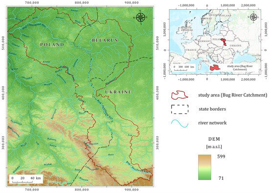
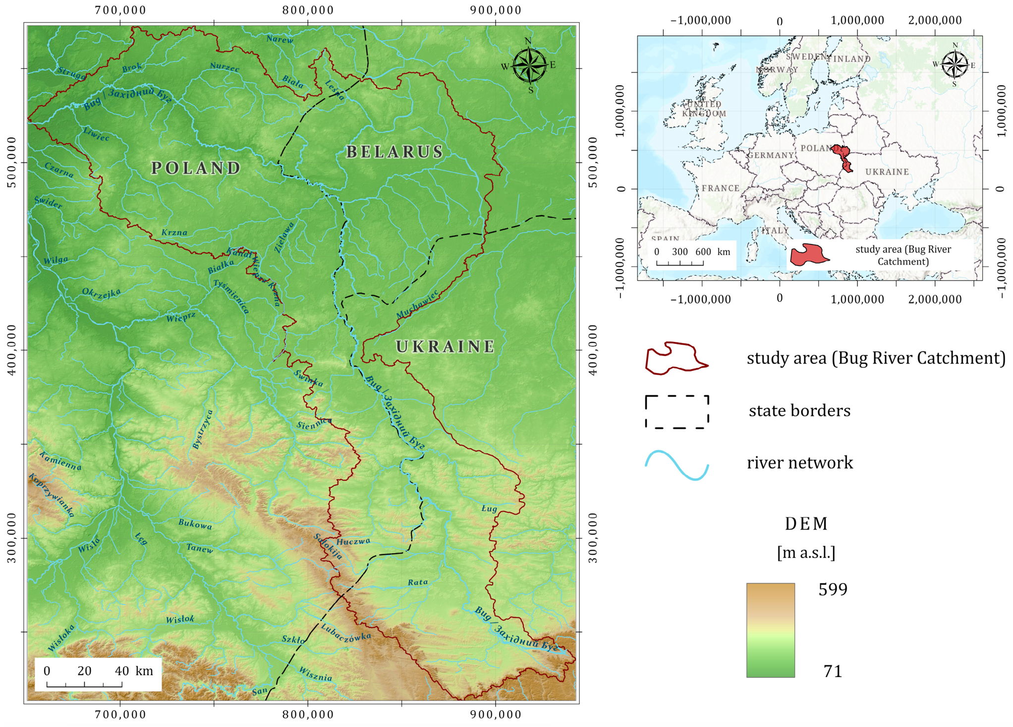
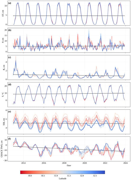
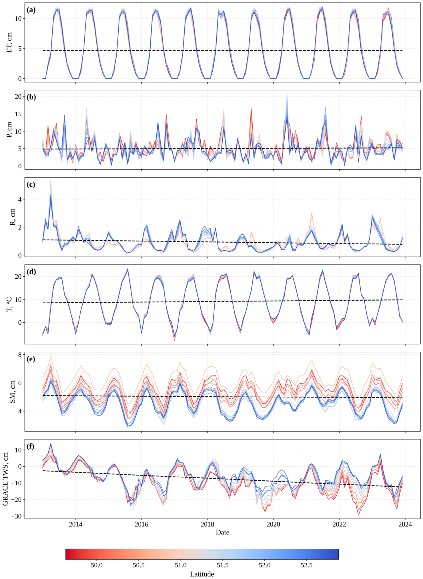
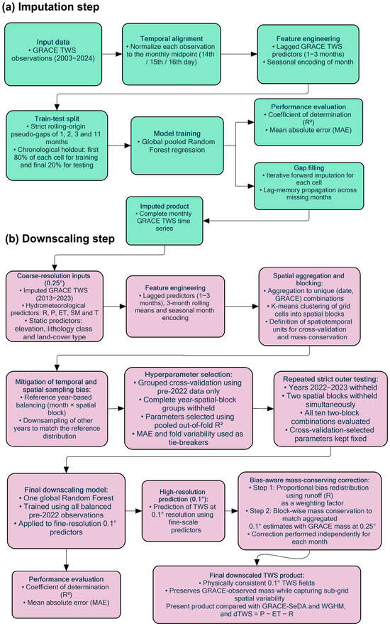
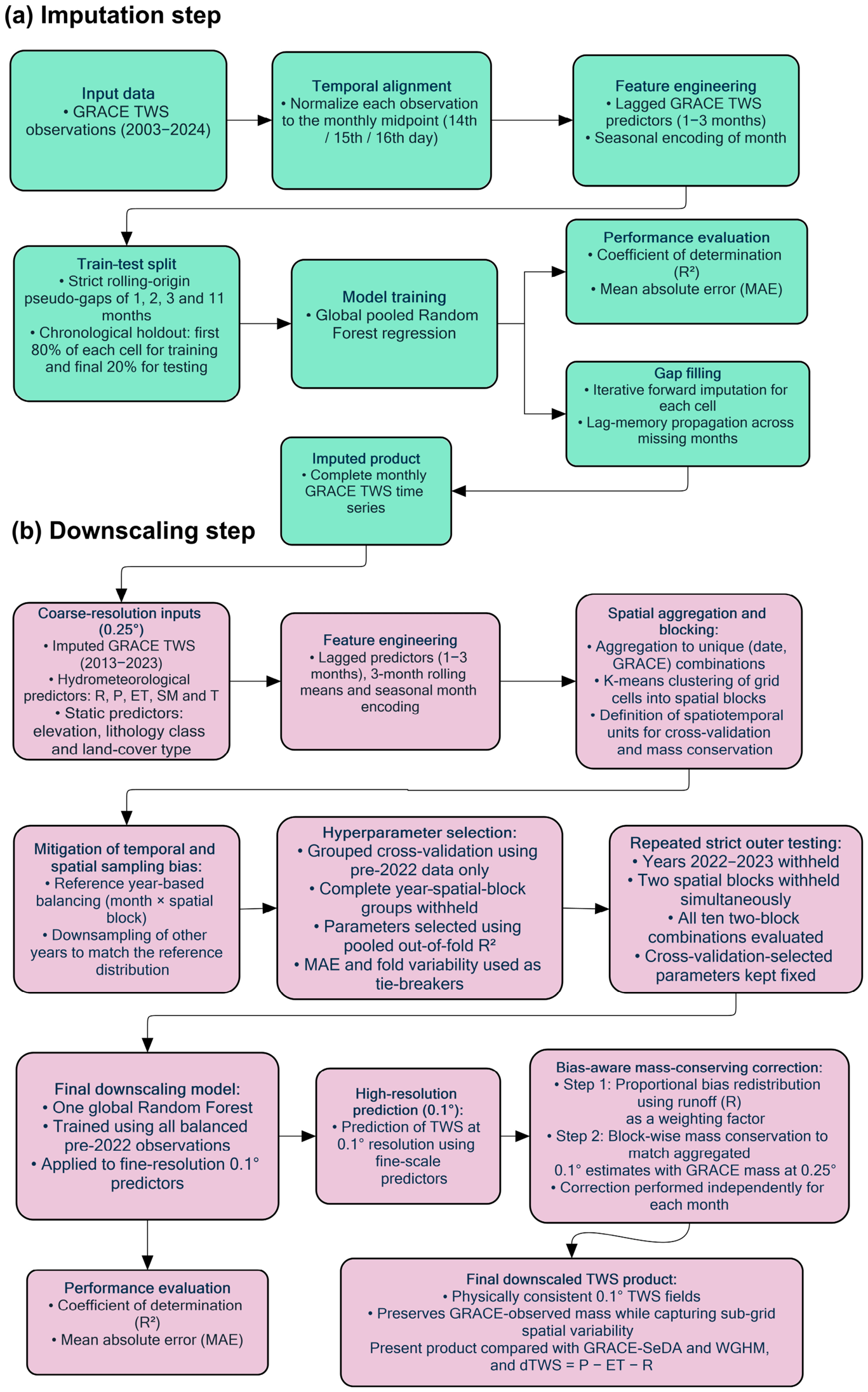
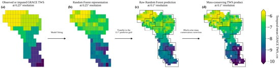
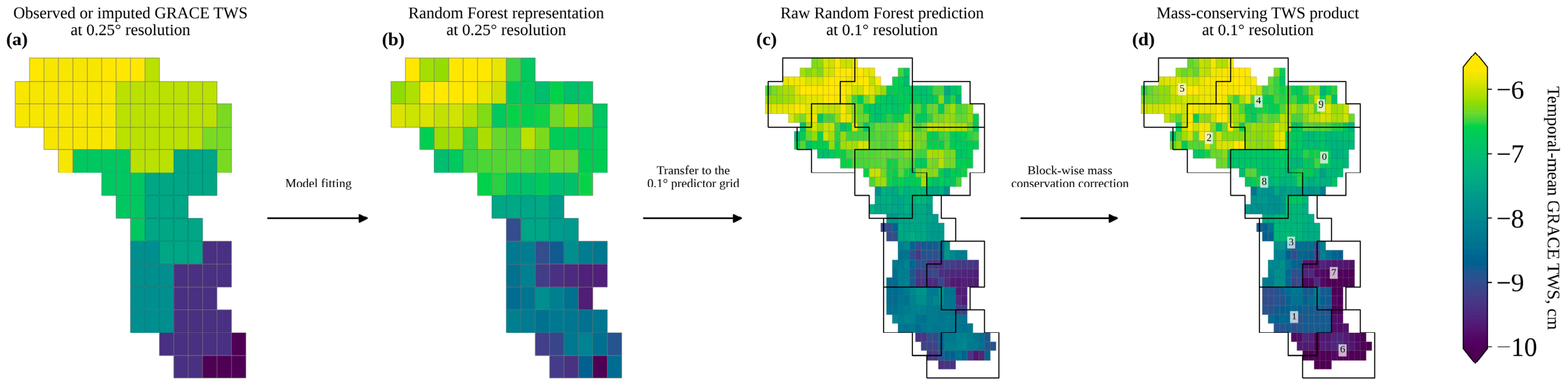
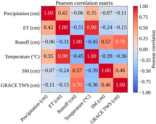
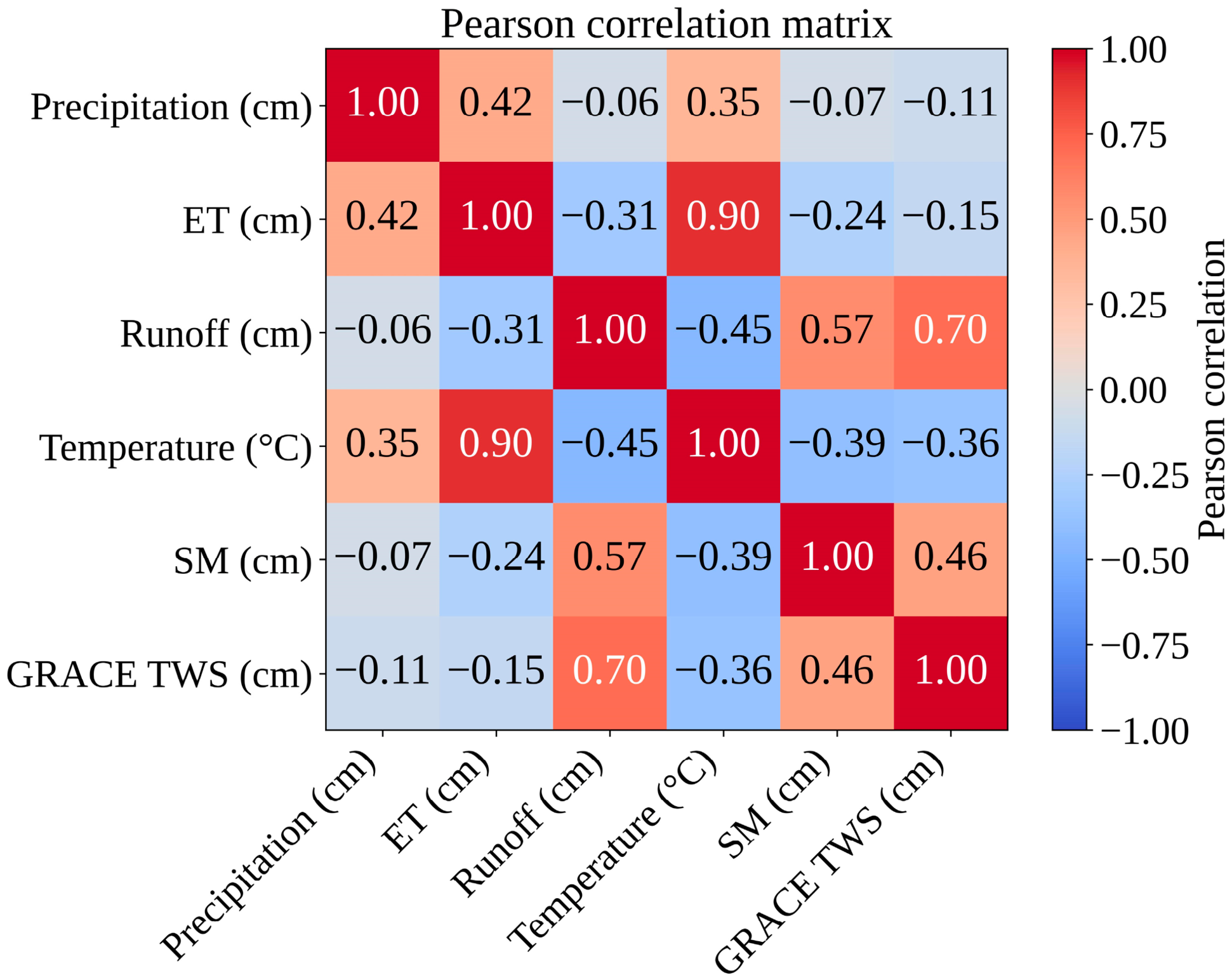
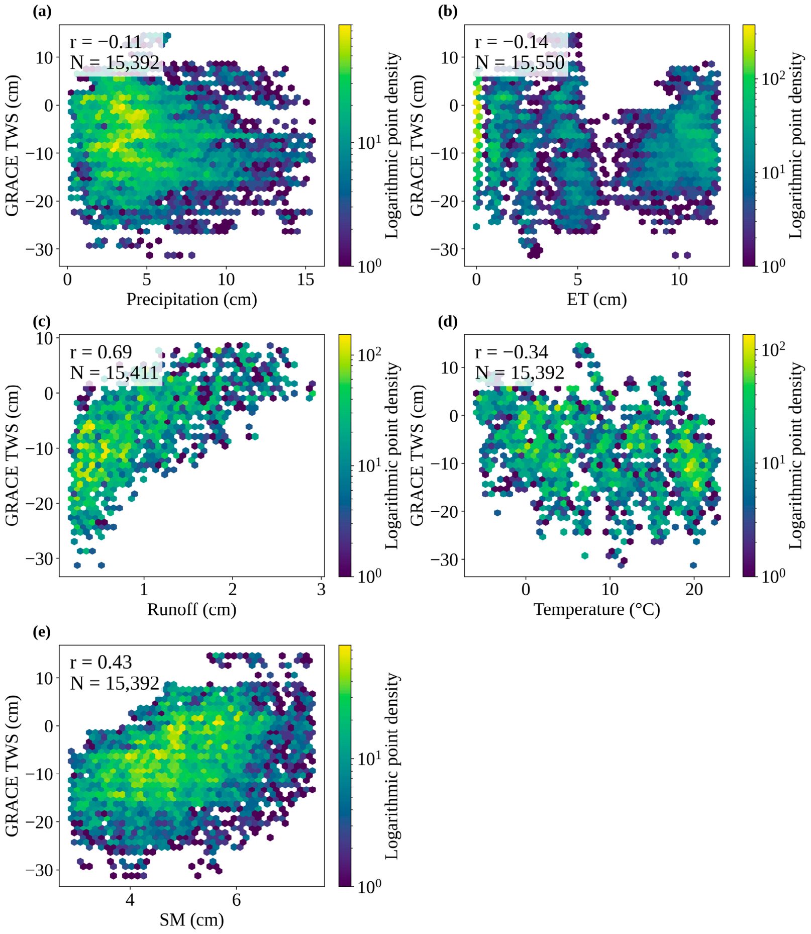
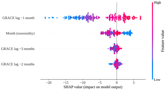
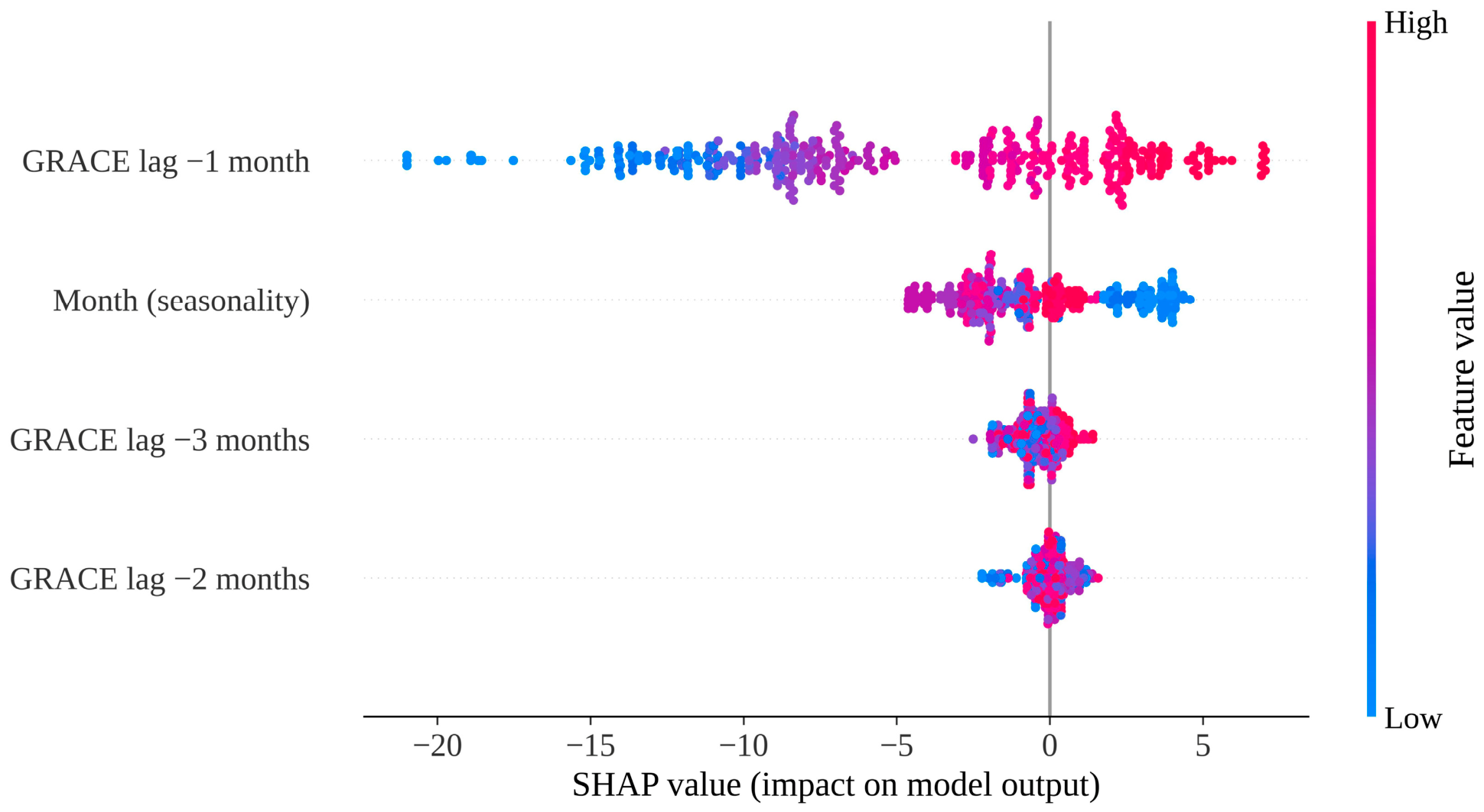
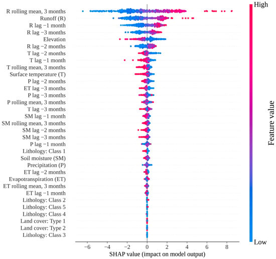
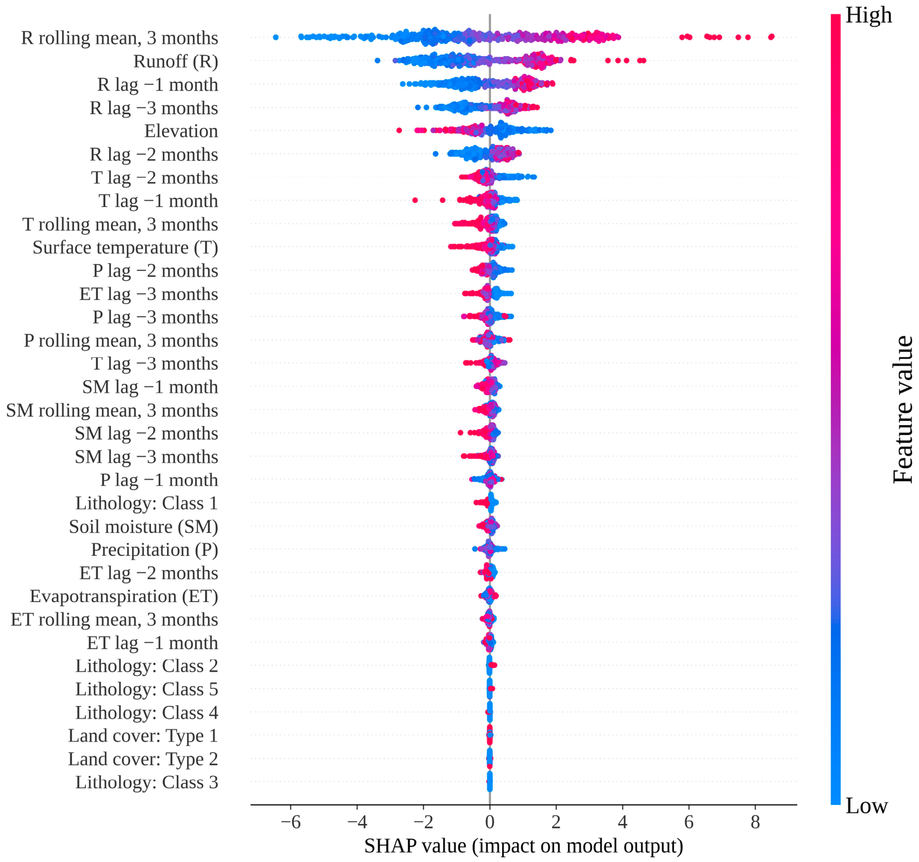
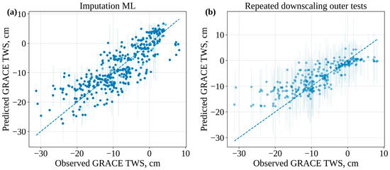
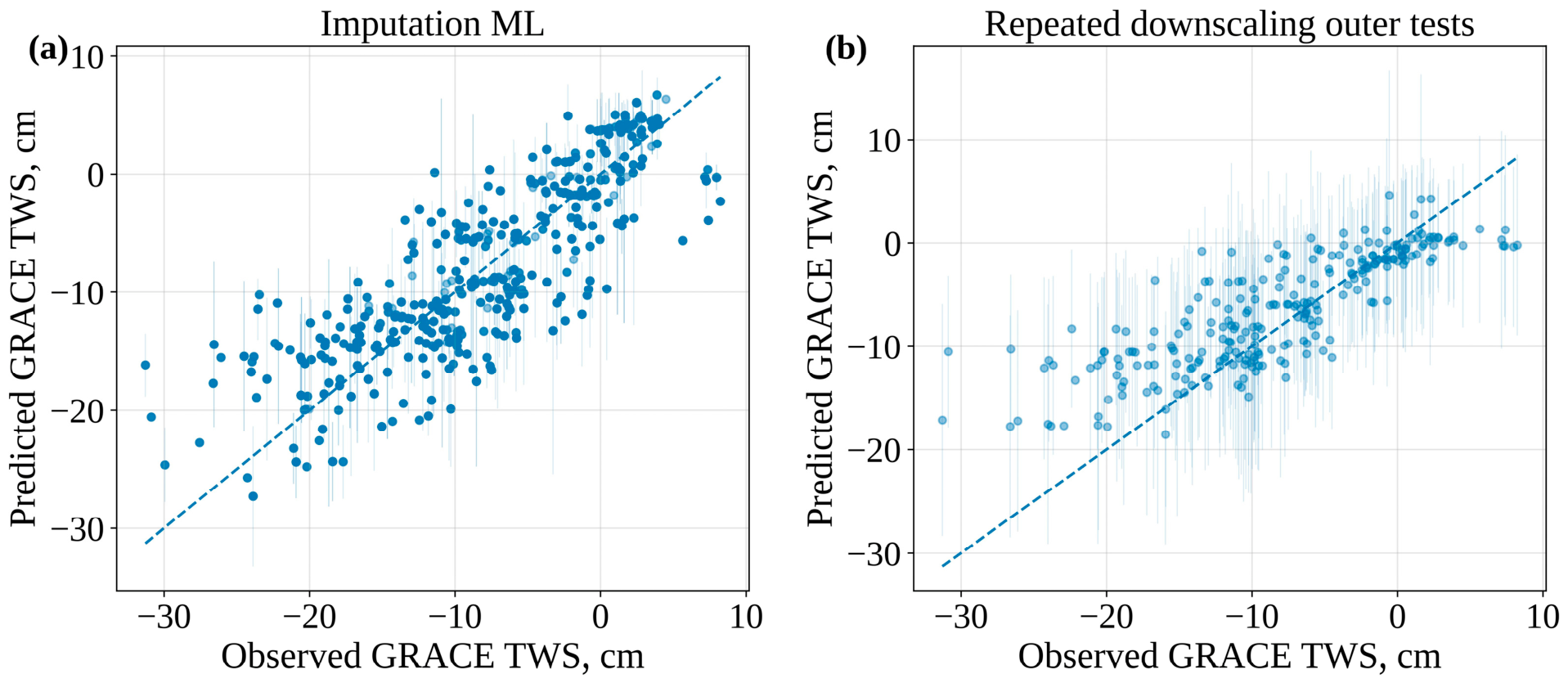
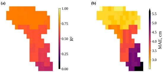
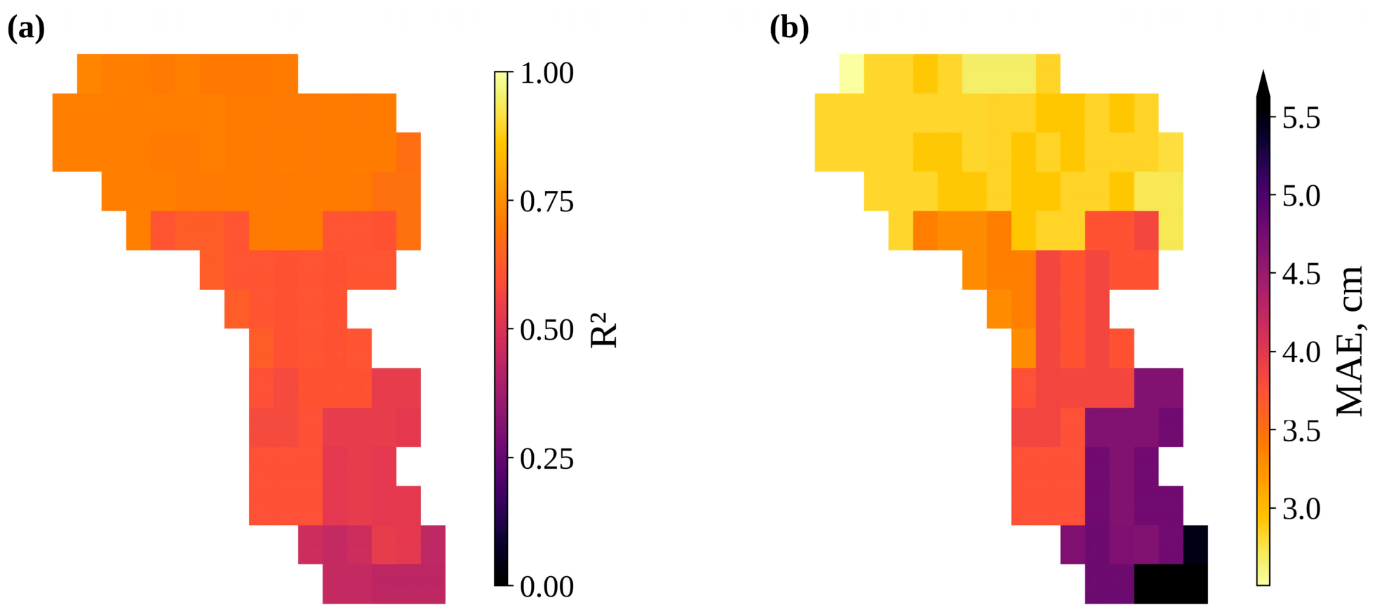
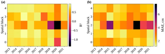
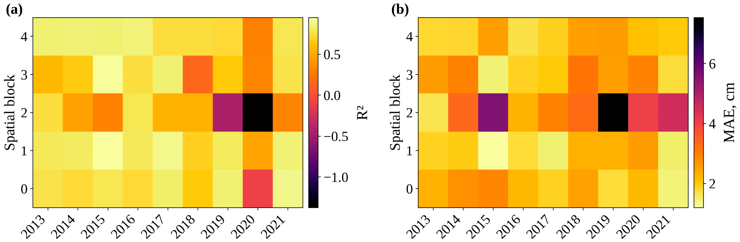
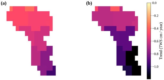
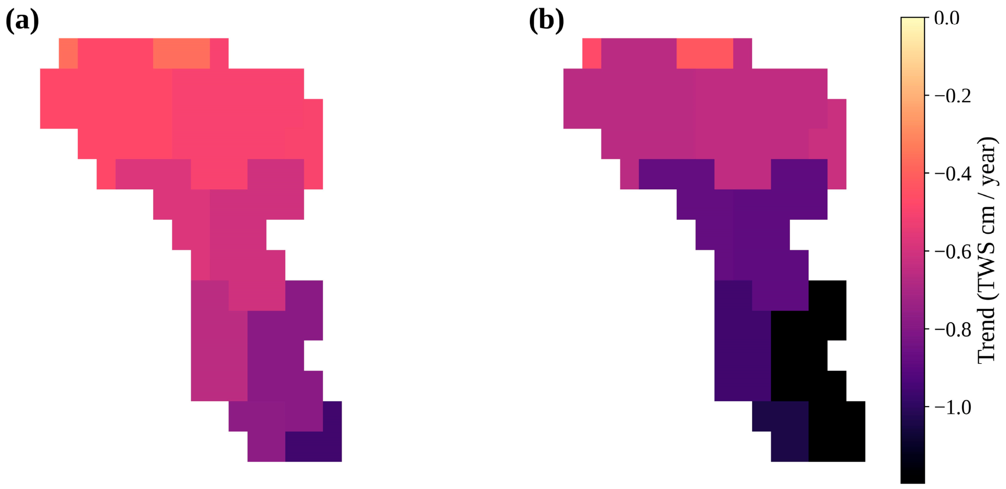
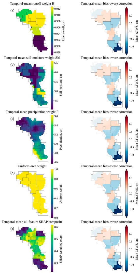
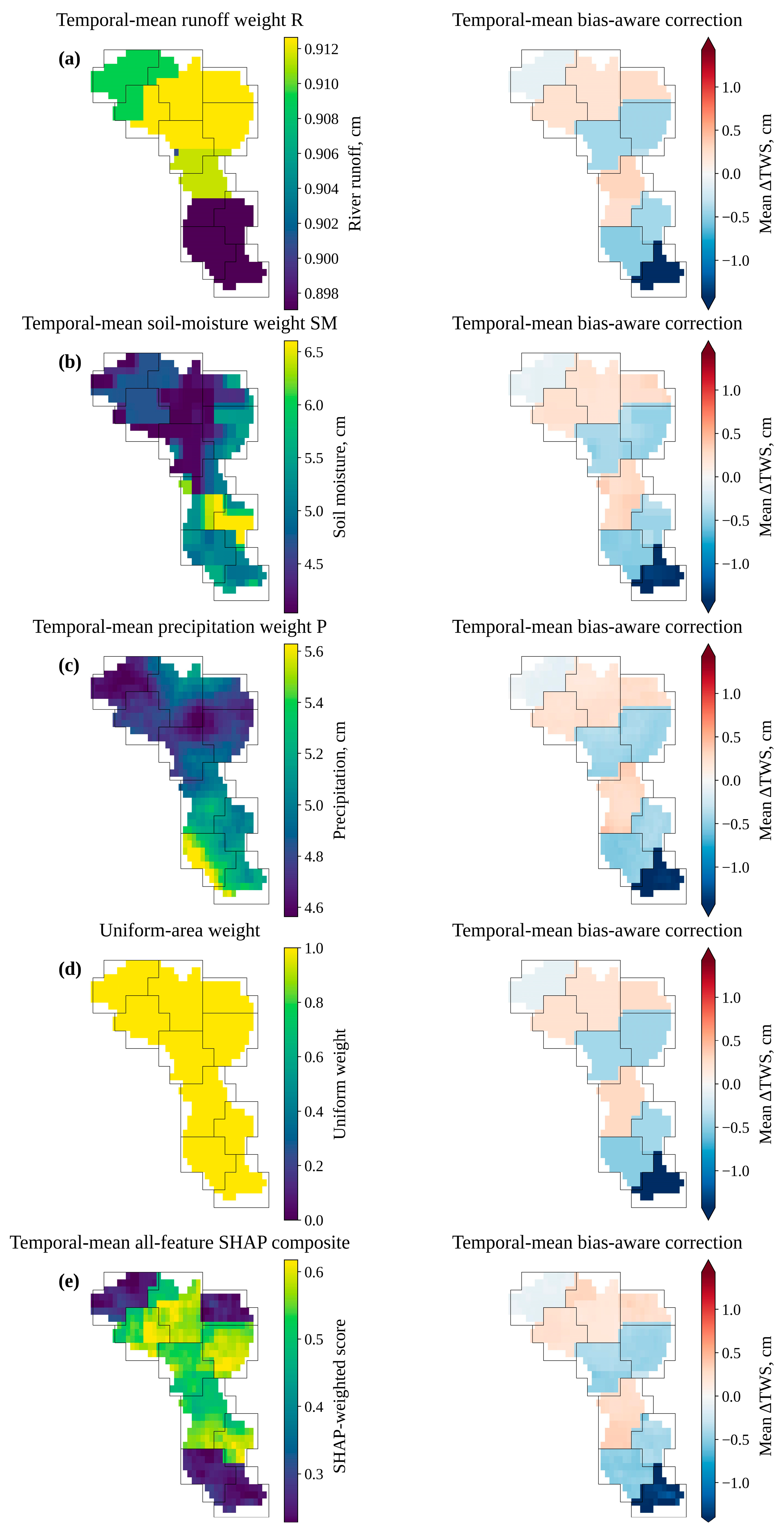
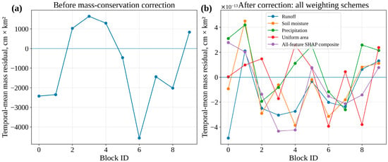
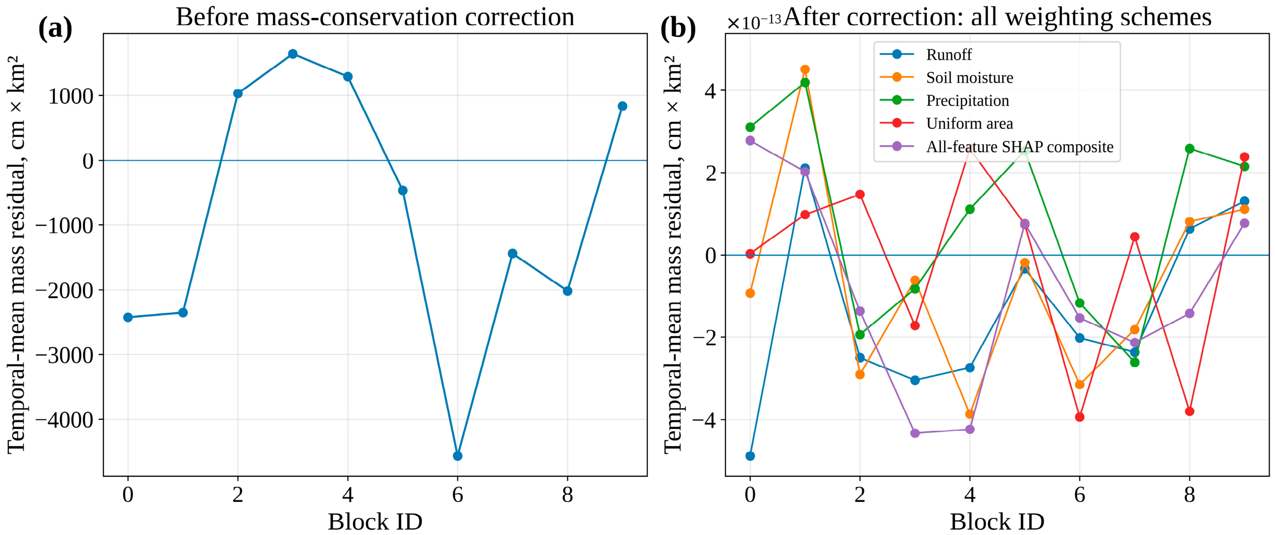
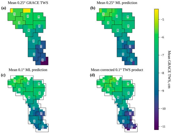
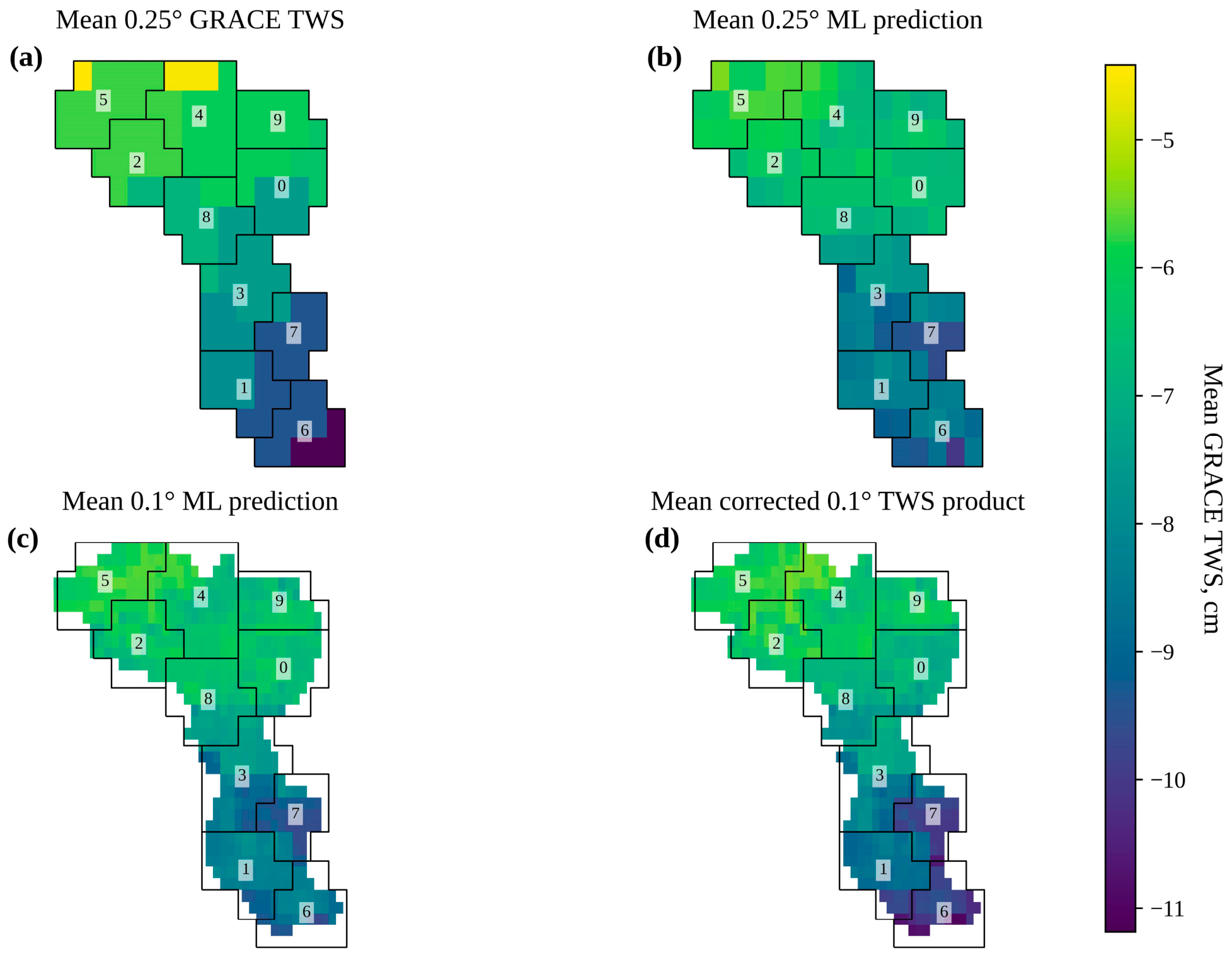
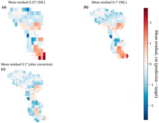
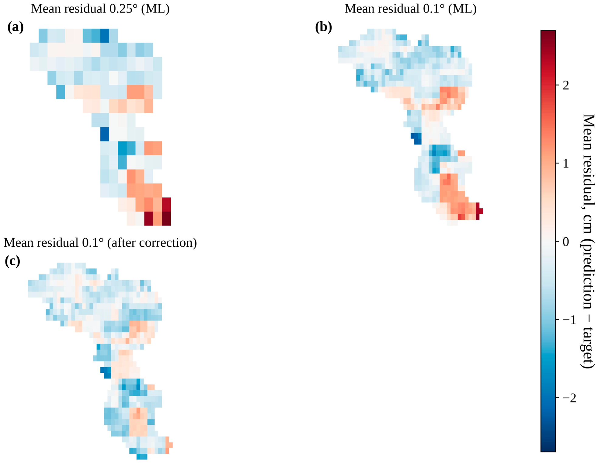
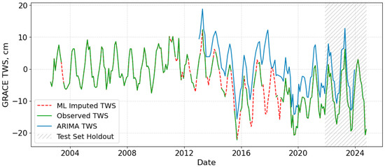
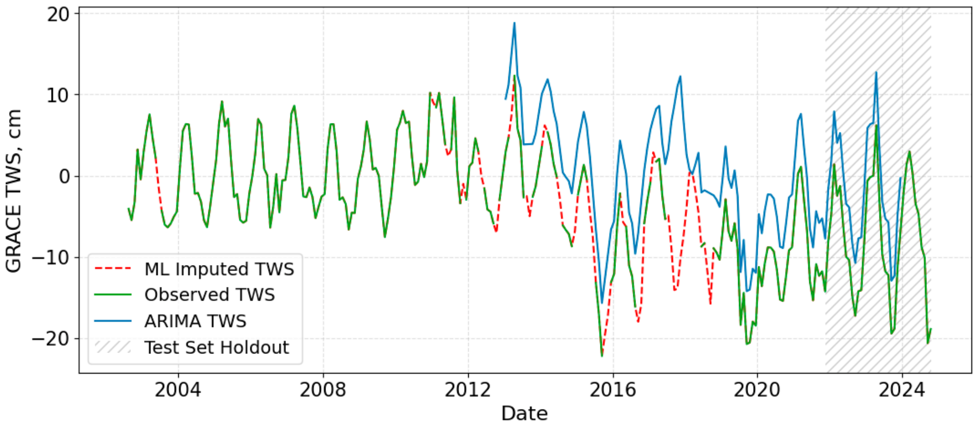
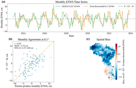
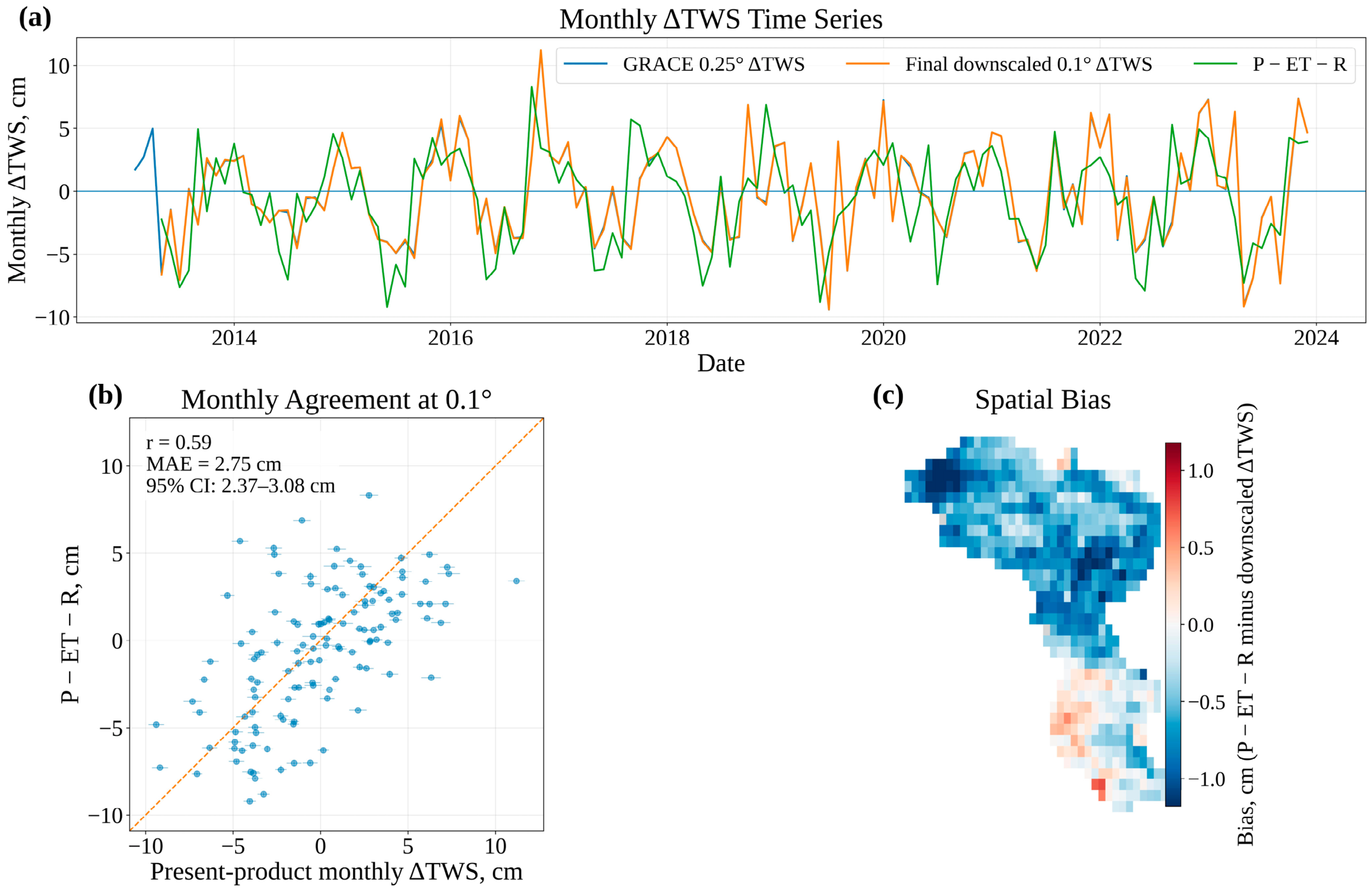
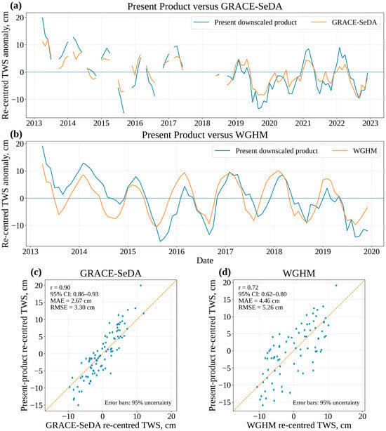
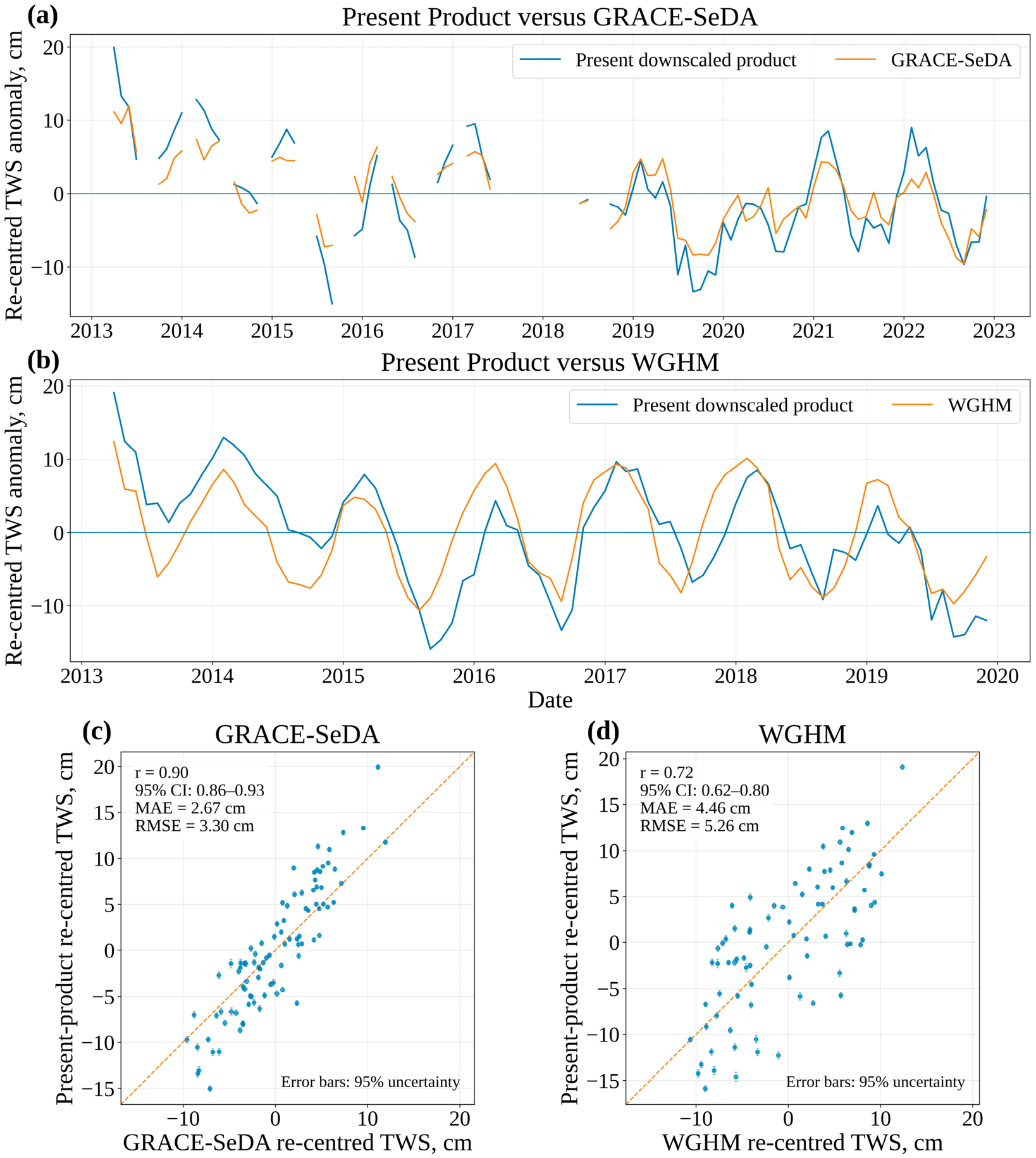
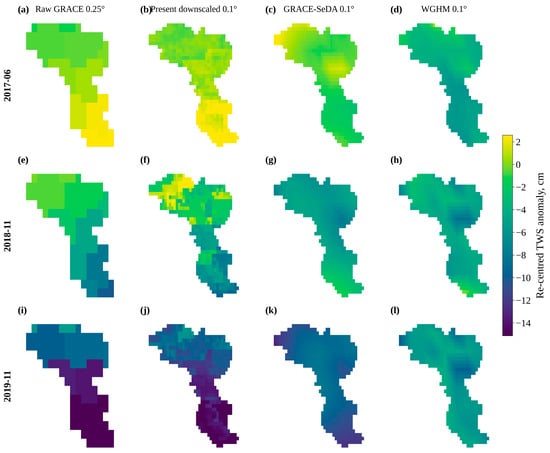
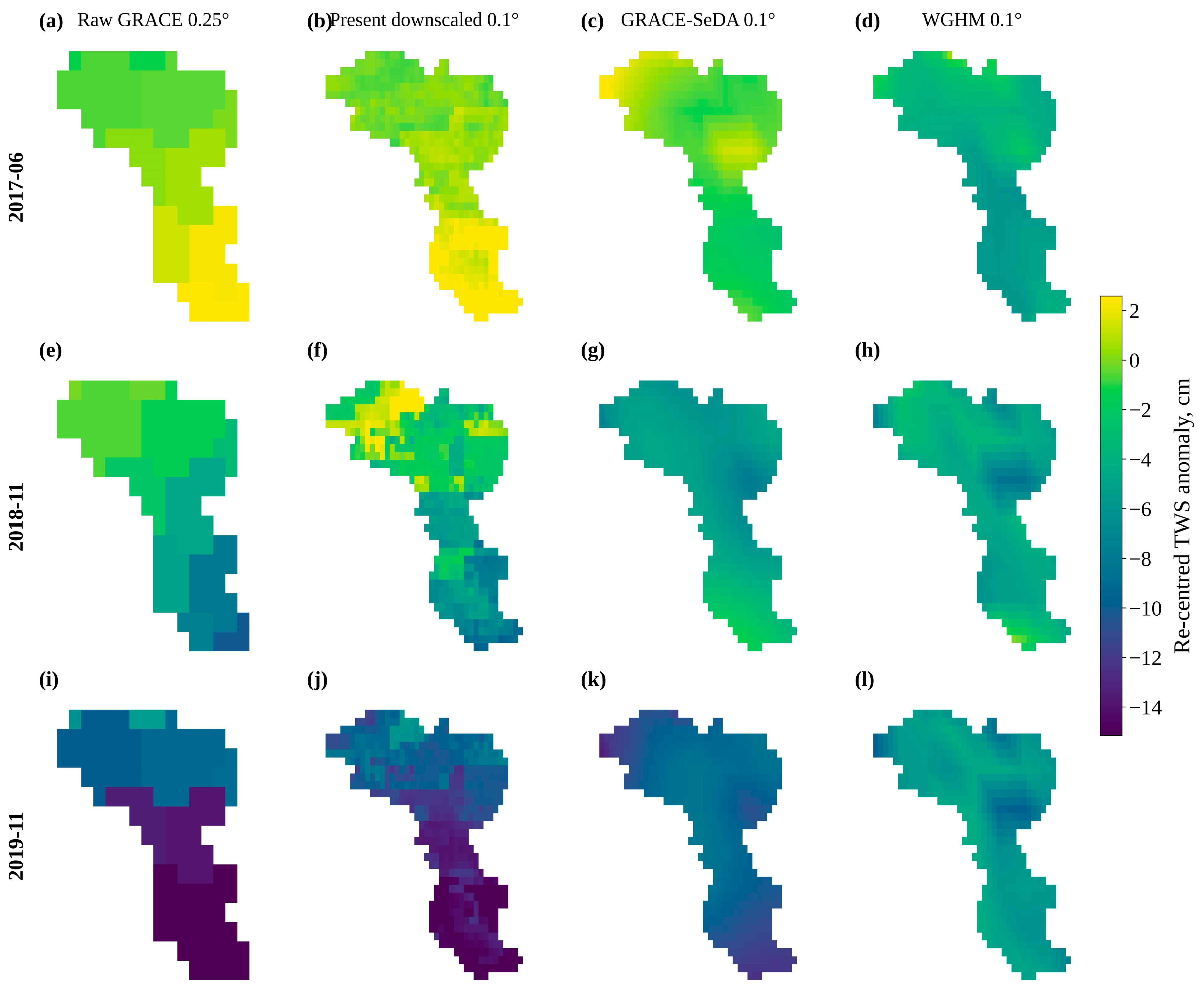

Disclaimer/Publisher’s Note: The statements, opinions and data contained in all publications are solely those of the individual author(s) and contributor(s) and not of MDPI and/or the editor(s). MDPI and/or the editor(s) disclaim responsibility for any injury to people or property resulting from any ideas, methods, instructions or products referred to in the content. |
© 2026 by the authors. Licensee MDPI, Basel, Switzerland. This article is an open access article distributed under the terms and conditions of the Creative Commons Attribution (CC BY) license.