


Highlights
What are the main findings?
- By fusing Sentinel-1 SAR, SWOT altimetry, and deep learning into a fully satellite-based framework, we reconstructed the Poechos Reservoir’s elevation–area–volume curve with high fidelity (NSE = 0.94) and no recurrent field campaigns beyond a single baseline bathymetric anchor, exposing an unrecorded, cumulative storage deficit of 24.5 hm3 in the active zone—averaging 3.5 hm3/year—that official records fail to capture.
- The framework reframes the satellite-versus-official volumetric bias as a direct, physically traceable proxy for active-zone sedimentation, converting a routine error metric into an operational sedimentation-auditing tool.
What are the implications of the main findings?
- Trained solely on Poechos, the model transferred zero-shot—without any retraining—to three morphologically distinct reservoirs (San Lorenzo, Tinajones, and Gallito Ciego), sustaining a 93.17% mean Intersection over Union (mIoU) and confirming that the approach generalizes across contrasting Andean–coastal settings at low marginal cost.
- Delivering all-weather updates every 21 days, the framework offers a low-cost, scalable alternative to sparse bathymetric surveys, enabling water managers in data-scarce regions to shift from outdated static assessments toward near-continuous, sub-monthly reservoir monitoring.
Abstract
Sedimentation is eroding the water security of reservoirs in hydrologically active basins: the Poechos reservoir (Peru) has lost 62% of its original 887.7 hm3 capacity in 48 years, yet its Elevation–Area–Volume (EAV) curve is refreshed only by bathymetric surveys at decade-plus intervals, compromising flood regulation and the water supply for over 100,000 ha of farmland. To close this gap, we propose an integrated, low-cost, fully reproducible framework that reconstructs the EAV curve from freely available satellite data: Sentinel-1 SAR (287 acquisitions, 2021–2026), PlanetScope imagery as ground truth (23 dates), and Surface Water and Ocean Topography (SWOT) altimetry (53 validated passes, 2023–2026). Water surfaces were delineated with a deep learning segmentation model (Feature Pyramid Network with an InceptionV4 encoder), selected among nine architecture–encoder combinations and calibrated to a 0.64 decision threshold, achieving a 90.66% Intersection over Union (IoU) and a 95.10% F1 score; a stochastic quantile mapping algorithm then asynchronously coupled the area and elevation series. The resulting EAV curve matched daily operational records from Peru’s National Water Authority (ANA) with high precision (NSE = 0.94, R2 = 0.96, and RMSE = 25.93 hm3); the residual bias (BIAS = −11.23 hm3) reflects active sedimentation unaccounted for in the official curve. This bias peaked at an accumulated deficit of 24.5 hm3 during the 2023–2024 hydrological year (3.5 hm3/year), of which up to 19.6 hm3 is attributed to the 2023 Yaku cyclone as a phenomenologically scaled upper-bound estimate (9.8–19.6 hm3 across 40–80% attribution fractions), since SWOT was not yet operational during the event. Updating every 21 days under any weather and requiring no new field campaigns beyond the baseline bathymetric anchor, the trained ensemble was further transferred zero-shot to three additional reservoirs (San Lorenzo, Tinajones, and Gallito Ciego), demonstrating a scalable path from infrequent static assessments to near-continuous, dynamic monitoring of water storage.
1. Introduction
Reservoir sedimentation is dismantling, silently and irreversibly, the infrastructure on which global water security depends [1,2]. Annual capacity losses of 0.5–1% [2,3,4]—already verified in 7245 reservoirs between 1999 and 2018 [5] and projected to accumulate to 26% across 47,403 dams by 2050 [6]—erode large dams that store 7000–8300 km3 of freshwater (twice the annual river discharge) and sustain irrigation, hydro power, urban supply, and flood control [7,8,9]. Beyond multi-billion-dollar replacement costs [1,10], this decline propagates cascading risks to downstream food, energy, and water security. The issue, exacerbated by extreme rainfall in high water-erosion basins like the tropical and Andean regions [2,3], highlights a critical bottleneck: the lack of sub-monthly, cost-effective, and deployable monitoring tools to quantify capacity losses as they occur and guide adaptive responses.
The Poechos reservoir (Chira River, Piura, Peru; 1976) epitomizes this crisis. With an original useful capacity of 887.7 hm3, it irrigates 100,000 ha, supplies one million inhabitants, and powers two hydroelectric plants [11], yet its capacity fell to 365 hm3 in 2018 (a 58.8% loss in 42 years) [11,12] and to 337 hm3 by December 2024 (>62%, with 8–23 m sediment layers in central zones) [13]. ENSO episodes raised sedimentation rates by 140% after 1997–1998 [11,12], aggravated by abrupt events like Cyclone Yaku (March 2023), whose persistent cloud cover hides real-time storage losses from optical monitoring. Operations therefore rely on outdated elevation–area–volume (EAV) curves, underestimating flood, irrigation, and safety risks [6,13]—a deficit representative of dozens of reservoirs across Latin America, South Asia, and Sub-Saharan Africa [2,6].
Conventional bathymetric surveys (multibeam or single-beam echosounders with differential GNSS) remain the gold standard for centimeter-accurate EAV curves and the baseline for flood control, water allocation, and dam safety [1,14], but they are incompatible with sub-monthly monitoring: they require partial drawdowns that conflict with irrigation and hydropower commitments [14]; their cost and logistics confine them to snapshots separated by years or decades, leaving most reservoirs in the developing world with outdated hypsometry [2,6,15], and their delivery latency precludes quasi-real-time responses to extreme sedimentation pulses [2,6]. Irreplaceable for absolute calibration, they thus leave a gap that only sub-monthly, all-weather, low-cost complements can fill.
Satellite alternatives face limits of their own. Optical missions (Landsat, Sentinel-2, and MODIS) reconstruct EAV curves by combining water areas [16] with altimetric levels [17,18,19] but fail under the persistent cloud cover of rainy Andean basins [20,21]. Sentinel-1 provides all-weather C-band imagery (10 m, 12-day revisit) in which open water’s low specular backscatter ( to dB) is unambiguous [22,23,24], and SWOT (launched December 2022) delivers the first Water Surface Elevation (WSE) series with centimetric uncertainty and a 21-day revisit for water bodies >∼1 km2 [25,26]. However, their fusion collides with orbital asynchrony (12 vs. 21 days), which standard temporal interpolation cannot resolve without mixing hydrological states. Elmi et al. [27] and Tourian et al. [28] showed that stochastic quantile mapping solves this distributional coupling for river discharge; its extension to reconstruct reservoir EAV curves from asynchronous SAR areas and altimetric elevations constitutes the central methodological gap addressed by this study.
The framework’s first link is accurate water delineation in SAR imagery, since the binary mask governs the reliability of the area series. Classical thresholding (Otsu, ISODATA, and Bmax-Otsu) succeeds in cloudy tropical basins [22,29,30] but degrades with geographic variability, speckle, and the water–sediment transitions typical of high-solid-load reservoirs [31]. Encoder–decoder architectures—U-Net [32], FPN [33], and nested variants [34]—systematically outperform it, reaching 75–76% Intersection over Union (IoU) [35] and 93% F1 with EfficientNet-B7-based models [31]. In Andean reservoirs like Poechos, with irregular borders and seasonal littoral sediment plumes, the encoder choice directly dictates the accuracy of the series feeding the quantile mapping; this study therefore evaluates nine architecture–encoder combinations (U-Net, U-Net++, FPN with ResNet-50, InceptionV4, and EfficientNet-B7).
These advances have not yet been integrated into a reproducible operational framework for dynamic EAV reconstruction, and three structural gaps persist: orbital asynchrony still lacks a formal statistical treatment that couples the marginal distributions of area and elevation without destroying information [27,28]; existing curves are validated against a single static bathymetry, blind to progressive sedimentation and abrupt event-driven losses [2,6]; and reliance on local calibration confines transferability to gauged basins, excluding hundreds of developing-world reservoirs without terrestrial networks [6,15]. These gaps define the space addressed by the present work.
To address these limitations, we propose a satellite-based framework that, once anchored by a single baseline bathymetric survey, requires no recurrent field campaigns for dynamic EAV curve reconstruction—reducing rather than eliminating the dependence on field data—demonstrated in Poechos but is transferable to any reservoir with Sentinel-1 and SWOT coverage and an available baseline survey. It combines (a) deep semantic segmentation of Sentinel-1 imagery (2021–2026), selecting the optimal architecture among nine encoder–decoder combinations under cross-validation [32,33,34] with PlanetScope reference masks [36]; (b) WSE series from SWOT’s KaRIn altimeter (2023–2026) under multi-criteria quality control and datum correction [25,37]; and (c) stochastic quantile mapping via Monte Carlo simulation, coupling both series without temporal interpolation and deriving the EAV curve with its uncertainty bands [27,28]. Operating at SWOT’s natural cadence (∼21 days), the specific objectives are: (i) to select the optimal segmentation architecture under high sedimentary dynamics; (ii) to reconstruct Poechos’ dynamic EAV curve (2021–2026) by integrating SAR and SWOT; (iii) to quantify capacity losses from progressive sedimentation and abrupt extreme events against daily operational records [38] reported to the National Water Authority; and (iv) to demonstrate the regional transferability of the complete framework via zero-shot EAV reconstruction for the San Lorenzo [39], Tinajones [40], and Gallito Ciego [41] reservoirs. Throughout this article, “continuous monitoring” is used strictly in this operational sense—regular, all-weather updates at the ∼21-day SWOT cadence—and not as a claim of gap-free hydrometric gauging.
2. Study Area and Data
2.1. Study Area
The study area comprises the Poechos Reservoir, in the binational Chira-Catamayo basin of the Piura region, northwestern Peru (4°32′S, 80°31′W) [11]; its location and spatial layout are shown in Figure 1, where terrain corresponds to a hillshade of the 30 m Shuttle Radar Topography Mission (SRTM) digital elevation model [42] and the maximum historical water extent to the JRC Global Surface Water product [16]. The reservoir regulates the water supply of the Chira-Piura irrigation system. The torrential regime of this transboundary basin and its extreme seasonal fluctuations produce highly variable water surfaces and intense sediment transport during episodic climate phenomena, accelerating siltation and complicating operational monitoring; these variable extents and the surrounding geomorphology constitute the baseline for the multi-sensor reconstruction of the Elevation–Area–Volume (EAV) curve via stochastic quantile mapping.
Figure 1.
Location of the study area and zero-shot transferability validation sites. (a) Poechos Reservoir (primary case study), along with the transboundary Chira-Catamayo basin boundary (Peru–Ecuador) and drainage network. (b) Regional context of the four reservoirs within Peru, with a South America locator inset. (c–e) Zero-shot validation reservoirs: San Lorenzo (c), Tinajones (d), and Gallito Ciego (e); their water extents were derived from Landsat-based classification masks. Coordinate reference system: WGS 84 (EPSG:4326).
While Poechos is the primary study case, three additional major reservoirs in northern Peru—San Lorenzo (Piura) [39], Tinajones (Lambayeque) [40], and Gallito Ciego (Cajamarca/La Libertad) [41]—were incorporated exclusively to validate the regional transferability of the methodology. Their contrasting morphologies, operational regimes, and landscapes along the Pacific drainage provide a robust scenario for a zero-shot evaluation of the trained ensemble and the stochastic mapping outside the Poechos domain.
2.2. Data Used
2.2.1. ANA Operational Volume Records
Daily reservoir storage records for Poechos Reservoir were obtained from the Autoridad Nacional del Agua (ANA) of Peru, as reported by the Proyecto Especial Chira-Piura (PECHP), the agency responsible for the operational monitoring of the reservoir. The dataset comprises daily volume observations expressed in cubic hectometers (hm3), reflecting the seasonal and interannual variability characteristic of the system. These records constitute the independent reference series used to validate the satellite-derived elevation–area–volume curve and to assess the volumetric performance of the proposed methodology, as described in Section 3.6.2 [43].
2.2.2. 2024 Bathymetric Survey
The bathymetric reference data used in this study were obtained from the topographic–bathymetric survey conducted in 2024 by Consorcio Poechos under contract with the Proyecto Especial Chira-Piura (PECHP) [13,44]. The survey was officially approved by PECHP through Resolución Gerencial N° 084/2025 [44], and its results were subsequently incorporated into the updated flood-season operating rules for the reservoir [45]. The survey determined a current storage capacity of 336.4 hm3 at an elevation of 103.00 m OLSA (Origen Local del Sistema de Alturas, i.e., Local Height System Datum), reflecting a reduction of approximately 62% relative to the original 1976 capacity of 887.7 hm3 at that same elevation, attributable primarily to sedimentation driven by sediment transport from the Chira River. Within the proposed methodology, the 2024 bathymetric curve serves as a structural anchor: it provides the datum correction between the SWOT altimetric reference (EGM2008) and the local OLSA elevation system and supplies the base volume () required to initialize the trapezoidal integration of the satellite-derived elevation–area–volume curve. A complete description of these procedures is provided in Section 3.4 and Section 3.8.
2.2.3. Sentinel-1 Data
Synthetic Aperture Radar (SAR) imagery from the Sentinel-1 mission [46] was used as the primary data source for surface-water monitoring over the Poechos Reservoir. A total of 287 scenes were acquired, spanning the period from January 2021 to March 2026, comprising two relative orbits: R91 (ascending pass, 156 scenes) and R40 (descending pass, 131 scenes), with an average revisit interval of approximately 6 days when both orbits are combined. All images correspond to the Interferometric Wide (IW) swath mode in Ground Range Detected (GRD) format, with both VV and VH polarizations at 10 m spatial resolution [47]. The annual distribution of acquisitions reflects the operational continuity of the Sentinel-1 constellation, with coverage increasing from 24 scenes in 2021 to a maximum of 101 scenes in 2025, consistent with the activation of the dual-orbit acquisition strategy from 2023 onward (Table S1, Supplementary Materials).
2.2.4. Surface Water and Ocean Topography (SWOT)
The primary dataset used in this study was derived from the Surface Water and Ocean Topography (SWOT) Level-2 High-Resolution Raster Lake Single-Pass Observations (SWOT_L2_HR_LakeSP_Obs) product distributed by NASA’s Physical Oceanography Distributed Active Archive Center (PO.DAAC) [25]. Observations were obtained from SWOT satellite passes 035 and 188 over the Poechos reservoir (Piura, Peru), covering the period from July 2023 to April 2026. Initially, a total of 79 observations were retrieved—37 from pass 035 and 42 from pass 188—providing water surface elevation (WSE) estimates with associated uncertainty metrics, geophysical corrections, and auxiliary quality flags. Following a quality filtering procedure described in Section 3.4, a final subset of 53 valid observations (35 from pass 035 and 18 from pass 188) was retained for analysis, ensuring the reliability and spatial representativeness of the WSE time series used throughout this study. A summary of these observations is presented in Table S2 (Supplementary Materials).
2.2.5. PlanetScope Multispectral Imagery
High-resolution multispectral imagery from the PlanetScope constellation [36] was acquired for 23 selected dates distributed across the study period. The AnalyticMS_SR surface reflectance product was used, which provides four spectral bands—blue, green, red, and near-infrared (NIR)—at 3 m spatial resolution, with orthorectification and radiometric correction applied by the provider. Dates were selected by prioritizing cloud cover below 5% over the reservoir extent and temporal proximity to Sentinel-1 acquisitions. These 23 scenes (summarized in Table S3, Supplementary Materials) served as the basis for generating high-accuracy binary water masks constituting the ground truth used to train and validate the deep learning segmentation models, following the processing pipeline described in Section 3.2.
2.2.6. Datasets for Regional Transferability Validation
To evaluate the zero-shot transferability of the framework, auxiliary time series and in situ records were compiled for San Lorenzo, Tinajones, and Gallito Ciego. No local high-resolution imagery was used to retrain or fine-tune the segmentation weights: 12 PlanetScope acquisitions (four per reservoir, selected across distinct storage levels to encompass maximum morphological variability) were reserved strictly as independent ground truth for the spatial metrics of the zero-shot segmentations, while the baseline bathymetries from the official technical reports of the National Water Authority [39,40,41] served exclusively to establish the initial reference volumes of the stochastic EAV reconstruction, mirroring the Poechos pipeline.
The validation dataset comprises 965 Sentinel-1 SAR GRD scenes (San Lorenzo: 287, January 2021–March 2026; Tinajones: 339; Gallito Ciego: 339), 168 SWOT WSE observations (74 passes from Tracks 035 and 188; 61 from Tracks 188 and 313; and 33 from Track 188, respectively), and the 12 PlanetScope reference images, all preprocessed with pipelines identical to those described in Section 2.2.3 and Section 2.2.4. Historical daily operational records (dates and stored volumes) extracted from the corresponding ANA repositories [39,40,41] constitute the empirical baseline for validating the reconstructed EAV curves. The complete acquisition inventories are provided in Tables S4–S12 (Supplementary Materials), mirroring Tables S1–S3 of the primary study area; public access to these datasets and to the zero-shot outputs is detailed in the Data Availability Statement.
3. Methodology
3.1. Overview of the Integrated Framework
The proposed methodology integrates three independent satellite data streams into a unified workflow for reconstruction of the Elevation–Area–Volume (EAV) curve of Poechos Reservoir without recurrent field campaigns once anchored to a single baseline bathymetric survey. Figure 2 summarizes the workflow in three sequential modules: Module I processes the 287 Sentinel-1 scenes (2021–2026) through a deep learning framework trained on PlanetScope-derived reference masks, producing a continuous area series at 10 m resolution; Module II applies a seven-criteria quality control to the 79 SWOT KaRIn observations, yielding 53 validated WSE estimates corrected to the local OLSA datum; and Module III couples both outputs through stochastic quantile mapping (Monte Carlo, ), bypassing the need for temporally coincident observations. The resulting curve, anchored to the 2024 bathymetric survey, is validated against ANA operational records () and interrogated for sedimentation signatures and extreme hydro-sedimentary events.
Figure 2.
Integrated methodological framework for satellite-based EAV curve reconstruction at Poechos Reservoir.
The framework assembles established building blocks—encoder–decoder segmentation networks [32,33,34], SWOT LakeSP altimetry [25], and quantile-based distribution matching [27,28]—but its contribution resides in five elements that, to the best of the authors’ knowledge, have not been previously reported: (i) the extension of stochastic quantile mapping from riverine discharge estimation to lacustrine EAV curves under multi-mission orbital asynchrony (Section 3.8); (ii) a reservoir-specific, seven-criteria quality-control protocol for SWOT LakeSP observations that discriminates swath-edge degradation from hydrodynamic turbulence (Section 3.4); (iii) a multi-criteria model selection and decision-threshold calibration protocol tailored to sediment-laden littoral margins (Section 3.5 and Section 3.6); (iv) the reinterpretation of the satellite-versus-official volumetric bias as a physically traceable proxy for active-zone sedimentation, with its attribution framework (Section 3.9); and (v) a zero-shot transferability protocol that validates the complete pipeline on unseen reservoirs without retraining (Section 3.10). The subsections below follow the operational order, indicating at each step which components are adopted from the literature and which are original.
3.2. PlanetScope Reference-Mask Generation
Reference binary water masks were generated from PlanetScope imagery (Section 2.2.5) via a two-stage thresholding pipeline. First, the Normalized Difference Water Index (NDWI; [48]) was computed from the green and near-infrared bands, and a conservative static threshold () was applied to capture water pixels in turbid, sediment-laden margins. Second, a spatially adaptive Bmax–Otsu algorithm resolved shoreline pixels by pooling sub-tiles with a between-class-to-total-variance ratio of to derive a locally representative threshold; sub-tiles lacking bimodality defaulted to a global Otsu value.
Both masks were merged by logical union to maximize shoreline recall and subsequently constrained by the JRC Global Surface Water maximum extent [16] to suppress commission errors. The resulting 3 m binary masks served as reference labels for deep learning training and accuracy assessment.
These masks constitute semi-automated reference labels rather than manually digitized, error-free ground truth. Each of the 23 masks was visually inspected against its source PlanetScope composite before entering the training pool, and candidate dates whose fused masks exhibited residual cloud, haze, or thresholding artifacts were discarded during the master-date selection (Section 2.2.5). Residual label noise concentrates in shallow, turbid, or sediment-rich margins, where water and saturated mud can be confounded, even at 3 m resolution; the NDWI–Bmax–Otsu union deliberately favors shoreline recall, while the JRC maximum-extent constraint bounds commission errors. The influence of this label uncertainty is therefore bounded rather than eliminated: all accuracy metrics reported hereafter quantify agreement with these reference labels, and their downstream volumetric impact is absorbed by the ensemble area dispersion () propagated through the stochastic mapping (Section 3.8) and revisited in Section 5.9. For brevity, the term “ground truth” is retained hereafter in this operational sense.
3.3. SAR Preprocessing and Dataset Construction
The 287 Sentinel-1 scenes were delimited by an area of interest derived from the maximum historical flood extent of the JRC Global Surface Water product [16], expanded with a perimeter buffer to capture the littoral transition zone so that the domain covered 100% of the historically recorded water surface without irrelevant surrounding land. All scenes were co-registered via bilinear reprojection to a master grid ( pixels), and the 23 PlanetScope masks were reprojected to the same template with nearest-neighbor interpolation to preserve binary values.
Each scene was encoded as a three-channel tensor: VV backscatter (dB), the primary water–land discriminator in the C band; VH backscatter (dB), sensitive to surface roughness and volumetric structure [49,50]; and the difference of (dB), a numerically stable separability index. Min–max normalization was computed globally across scenes, restricted to the area of interest to avoid the statistical dominance of land pixels, and mapped to —reserving for pixels outside the domain or flagged as invalid (layover shadows, and non-finite values)—so the model unambiguously separates valid signal from background.
3.4. SWOT Data Processing and Datum Correction
Water surface elevation (WSE) observations were obtained from the SWOT_L2_HR_LakeSP_obs_D product (PO.DAAC/NASA), referenced to the EGM2008 geoid, from two passes with contrasting geometry: Pass 035 covers the main body in front of the dam under favorable mid-swath conditions (≈16 km from nadir, ), while Pass 188 covers the reservoir tail at the swath edge (≈59 km, ). After removing duplicates from the initial 79 observations (July 2023–April 2026), a seven-criteria quality control retained only physically representative estimates: C1 (), unconditional rejection in both passes; C2 (), signal dominated by saturated soil or emergent vegetation; C3 ( m, Pass 188 only), water–land mixing at the tail (Pass 035 is exempt because its high during extreme droughts reflects surface turbulence, and removing it would erase the lower percentiles needed by the quantile mapping); C4 ( m), crossover calibration bias comparable to the seasonal signal; C5 (Pass 188 with m), tail exposed over the alluvial fill, with WSE reflecting topography rather than the free surface; C6 (, Pass 188 only), degraded quality compounded by swath-edge geometry; and C7 ( m, Pass 035 only), instrumental anomalies beyond any physical turbulence. The protocol retained 53 validated observations (Track 035: 35; Track 188: 18; Table S2, Supplementary Materials), spanning 95.5 to 105.5 m a.s.l.
The SWOT datum correction (EGM2008 → local topographic datum OLSA) computed, for each observation with a simultaneous volume record from the Chira Piura Special Project (PECHP) [43] reported to the National Water Authority (ANA), the individual offset () via inverse interpolation on the 2024 bathymetric curve; the global offset (, the arithmetic mean of all ) was then added to the complete WSE series as a constant. This offset is compared against the one obtained in the 2024 bathymetric study by Consorcio Poechos [13] as an independent external validation. The base volume (, the permanent storage below the minimum SWOT-observable elevation, already in the OLSA datum) was extracted from the same bathymetric curve and incorporated as the integration constant of the EAV reconstruction (Section 3.8). It must be emphasized that this datum correction performs a constant vertical registration between reference frames: it shifts the SWOT elevations by the single scalar of and recalibrates neither areas nor volumes. Consequently, it cannot transfer any volumetric bias to the pre-2024 satellite predictions, and it is mathematically independent of the historical operational curve later used as the comparison baseline for the systematic bias (BIAS) (Section 3.6.2 and Section 5.9).
3.5. Deep Learning Model Selection and Training
A strict spatio-temporal partitioning strategy governed model construction and evaluation. The experimental dataset was built from 23 master dates (Table S3, Supplementary Materials) featuring simultaneous cloud-free PlanetScope imagery and Sentinel-1 acquisitions; for each date, the PlanetScope-derived binary mask and the co-registered three-channel SAR tensor (VV, VH, and VV-VH) were partitioned into 122 non-overlapping patches of pixels.
Three complete dates (366 patches) were isolated as an external hold-out never seen during any training phase, and the remaining 20 dates (2440 patches) fed a stratified 5-fold cross-validation. Stratification balanced the reservoir’s hydrological states (low, medium, and high water levels) across folds, and the splits were segregated by date groups to prevent spatio-temporal leakage between training and validation subsets: each fold combined 16 dates (1952 patches) for internal training with 4 distinct dates (488 patches) for internal validation.
Three architectures—U-Net [32], U-Net++ [34], and Feature Pyramid Network (FPN) [33]—were each paired with three convolutional encoders—ResNet-50 [51], Inception-v4 [52], and EfficientNet-B7 [53]—forming a matrix of 9 combinations and, under the 5-fold scheme, 45 independently trained networks. All encoders were initialized with ImageNet pre-trained weights [54] to leverage transfer learning.
Training ran for up to 50 epochs (batch size of 16) with the Adam optimizer [55] (initial learning rate of ), minimizing the binary cross-entropy with logits loss, and early stopping (patience 15 epochs) monitored the mean Intersection over Union (mIoU) on internal validation. The optimal combination, identified through the multi-criteria ranking across folds was then used for continuous inference over the 287 Sentinel-1 scenes. The framework was implemented with the Segmentation Models PyTorch library (v0.5.0) [56] on an NVIDIA H100 Tensor Core GPU (NVIDIA Corporation, Santa Clara, CA, USA); the H100 was required only for this one-time training, and the released ensemble weights (Data Availability Statement) reduce operational deployment to forward inference on commodity GPUs, without retraining.
3.6. Model Evaluation
3.6.1. Segmentation Model Evaluation
Segmentation accuracy was assessed under the 5-fold cross-validation strategy [57], using a standard panel of semantic segmentation metrics [58] computed from the confusion matrix against the PlanetScope reference masks: mean Intersection over Union (mIoU); F1 score (Dice); precision; recall; global accuracy; and Cohen’s Kappa (), which accounts for chance agreement [59].
To select the definitive model among the 9 combinations (45 trained networks), a 4-phase hierarchical ranking was applied: (1) mean mIoU across folds, the most stringent geometric metric since it penalizes false positives and false negatives simultaneously; (2) F1 score, balancing precision and sensitivity; (3) recall, prioritizing detection of all water pixels; and (4) mIoU standard deviation (IoU std) as the training stability criterion.
Finally, because the output layer produces continuous probability maps through a sigmoid, the binarization threshold was calibrated rather than fixed at the default 0.5: a grid search jointly maximized mIoU and F1 score over the fold validation sets [60], empirically establishing the decision boundary used for the inference of the complete time series.
Additionally, to quantify the practical gain of deep learning over classical SAR water-delineation methods, two threshold-based benchmarks were evaluated on the identical external hold-out set: a global Otsu threshold applied to Gaussian-smoothed VV backscatter ( pixels) and an ISODATA classifier applied to the raw signal [22,23]. Their results are reported alongside the deep learning ensemble in Section 4.1.5 and interpreted in Section 5.1.
3.6.2. Comparative Evaluation of the EAV Curve and Volumetric Discrepancy
The hydrological coherence of the satellite-derived EAV curve was evaluated against the in situ daily operational volumes administered by the National Water Authority (ANA). Because this research posits that the official capacity curve underestimates the continuous loss of useful volume to sedimentation, the ANA records were never assumed to be absolute, error-free ground truth. The evaluation therefore combines two complementary readings: (1) hydrological dynamics via the Nash–Sutcliffe efficiency (NSE) and the coefficient of determination (), verifying that the satellite prediction replicates the temporal variance of filling and emptying [61], and (2) error magnitude via the root mean squared error (RMSE), its normalized form (NRMSE), and the systematic bias (BIAS) [38]. Under this framework, the systematic negative divergence between the satellite estimate (which scans the current physical surface) and the operational record (based on theoretical capacity) is not an algorithmic failure but the direct quantitative estimator of the volume lost to unrecorded siltation.
This design choice raises a legitimate question of circularity—validating against a record whose capacity curve the study itself declares outdated—that deserves an explicit answer. The ANA operational volumes are generated by projecting instrumentally accurate daily gauge elevations onto the official capacity curve: their temporal dynamics (filling and emptying trajectories) are therefore reliable, while their absolute magnitudes inherit the systematic error of the underlying curve. Accordingly, the dynamic metrics (NSE, ) validate exclusively the temporal coherence of the satellite reconstruction, and at no point are the ANA volumes treated as absolute volumetric truth; the magnitude metric (BIAS) is read inversely as an estimate of the reference curve’s own obsolescence. Two independent elements break the apparent circle: the datum correction is a pure vertical registration that cannot inject a volumetric signal (Section 3.4), and the abrupt inversion of the bias immediately after the official adoption of the 2024 bathymetry (Section 4.6) behaves exactly as the sedimentation interpretation predicts and as no algorithmic artifact would.
3.7. Water Surface Area Inference and Time Series
To reconstruct the surface dynamics over 2021–2026, the 287 full scenes were processed with a soft-voting ensemble of the five validated fold models. Because inference on tensors is prone to GPU memory limits and seam artifacts at prediction boundaries, a sliding-window procedure with Gaussian blending was implemented [32,56,58]: patches of pixels were extracted with a 128-pixel stride (50% overlap), and the contribution of each pixel to the global probability map was modulated by a two-dimensional Gaussian kernel ( pixels), which weights the statistically more robust patch center over the margins. The continuous probability map () is the weighted average of the probabilities predicted by the K overlapping patches:
where is the probability predicted by the ensemble for patch k and is the Gaussian kernel coefficient at that position.
Binarization employed the calibrated decision threshold (Section 3.6.1) rather than the standard 0.5 cutoff, discriminating shallow, turbid littoral zones and mitigating commission errors under high sediment loads. The water surface area of each date () follows algebraically from the count of positively classified pixels times the nominal resolution (), and the inter-ensemble standard deviation () across the five folds quantifies the model’s epistemic uncertainty, defining the dynamic confidence interval () propagated into the stochastic coupling with the altimetric series.
3.8. Stochastic EAV Curve Reconstruction
To couple the asynchronous time series of the water surface area (derived from the Sentinel-1 ensemble inference) and the water surface elevation (WSE, derived from SWOT), a non-parametric stochastic quantile mapping algorithm was implemented [27]. The fundamental premise of this approach is that both the spatial extent of the water mirror and its elevation are governed by the identical underlying hydrological state of the reservoir. Consequently, under the assumption of a monotonic relationship, the k-th percentile of the area distribution strictly corresponds to the k-th percentile of the elevation distribution. This facilitates continuous hypsometric curve reconstruction without the necessity of simultaneous satellite overpasses [28]. The monotonicity premise is not merely postulated: it was verified empirically by pairing, without any statistical mapping, the Sentinel-1 areas acquired within ±3 days of each validated SWOT pass (results in Section 4.4); transient departures during rapid inflow are examined in Section 5.9.
The framework explicitly propagates three primary sources of observational uncertainty through a Monte Carlo simulation ( realizations):
- (Area uncertainty): Quantified as the standard deviation of the area estimates across the five folds of the FPN-InceptionV4 ensemble (Std_Folds_ha).
- (Elevation uncertainty): Derived from the KaRIn instrument’s intra-polygon standard deviation (wse_std), which captures the WSE heterogeneity within the SWOT observations.
- (In situ volume uncertainty): Initially set to a conservative prior of 10% of the daily operational volumes reported by the National Water Authority (ANA) and updated iteratively. This prior only initializes the convergence loop, which re-estimates from the residuals at every iteration; the converged value (7.69%; Section 4.4) is therefore driven by the data rather than by the initial assumption.
For each Monte Carlo realization (i), perturbed area (), and elevation (), series were generated by adding heteroscedastic Gaussian noise () to the base observations. To prevent physically impossible states, perturbed areas were truncated at 0.1 km2 and elevations at 90 m a.s.l.—5.5 m below the minimum SWOT-recorded elevation (95.48 m a.s.l., OLSA) of more than 12 given the mean elevation uncertainty m. Then, 200 equally spaced percentiles () were extracted from both distributions to form the and vectors, and the final mean elevation–area curve was obtained by averaging the 200 quantile pairs across the 500 realizations.
To compute the volumetric capacity, the stochastic elevation–area curve was numerically integrated using the trapezoidal rule:
where represents the dead storage volume below the minimum observable SWOT elevation, anchored to the 2024 local bathymetric survey [13].
Finally, an iterative convergence loop was executed to dynamically adjust the volumetric uncertainty () and capture the systematic bias induced by progressive capacity loss (siltation). In each iteration, satellite-derived volumes were compared against the interpolated ANA operational volumes. The Monte Carlo generation and numerical integration were repeated—updating the random seed for strict reproducibility—until the change in the Root Mean Square Error (RMSE) between consecutive iterations fell below the mathematical convergence threshold of 0.01 hm3, capped at a maximum of 15 iterations [27]. The ensemble size () and the 200-percentile grid were retained after the sensitivity checks summarized in Section 5.9, which bound the effect of halving or doubling N on the resulting 95% confidence intervals.
3.9. Sedimentation Rate and Extreme Event Detection
To contextualize the satellite-derived capacity loss, the active-zone sedimentation rate is benchmarked against the reservoir’s total physical rate: based on the operational records from commissioning to the most recent comprehensive bathymetric survey by PECHP and Consorcio Poechos [13], the long-term total is 11.48 hm3/year, the official denominator for quantifying which fraction of the sediment load settles within the active operational volume.
The systematic volumetric bias—the residual between the satellite-derived capacity and the operational records—was used as the indicator of sedimentation-induced storage loss, characterized through a two-dimensional sensitivity analysis:
- (1)
- Morphological Sensitivity: Residuals are partitioned by the physical state of the reservoir, using the median surface area to separate high-water phases (submerged sediments) from low-water recession (exposed sediments). This matters because coarse sediments settle preferentially within the active operational elevations—the live storage—whereas fine suspended particles deposit diffusely in the dead storage over a much longer timescale. Complementarily, the morphological error signature was derived by fitting a second-degree polynomial to the residuals as a function of water surface elevation (), identifying the elevation range where the bias is strongest and linking it to the differential exposure of sediment deposits.
- (2)
- Hydrometeorological Interannual Sensitivity: To reflect the stochastic nature of Andean sediment transport, the dataset is stratified into Hydrological Years (September–August), computing the localized bias and RMSE per cycle and isolating extreme events from baseline sedimentation trends [12].
The operative sedimentation rate () is derived from the mean volumetric bias of the Hydrological Year exhibiting the largest detected deficit (2023–2024) as follows:
where is the mean residual of the SWOT overpasses corresponding exclusively to the 2023–2024 cycle and years corresponds to the operational latency interval elapsed between the reference bathymetric survey (2017) and the most recent available survey (2024), a parameter adopted as an assumption external to the analysis, given that no intermediate field campaign was conducted to monitor the progression of sedimentation during that period [14]. By restricting the numerator to the year of maximum anomaly, the methodology quantifies the maximum accumulated deficit in the operational storage volume attributable to the period without bathymetric monitoring.
Additionally, a geomorphological attribution framework assesses the differentiated impact of extreme climatic anomalies on the total deficit. Grounded in the non-linear dynamics of fluvial sediment discharge () [14] and in the geomorphological Pareto principle—high-kinetic-energy events mobilize the dominant fraction of the multi-annual sediment load [62,63]—the protocol assigns an upper-bound attribution of 80% of the maximum detected bias to the extreme pulse of Cyclone Yaku (2023). Since SWOT began operating in July 2023, four months after the event, this factor cannot be derived from the satellite series; it is a physically informed estimate grounded in regional evidence: Morera et al. [63] documented that during extreme El Niño episodes (1968–2012)—the closest discharge analog, acknowledging Yaku’s distinct meteorological mechanism—annual suspended sediment yield rises by a factor of 3 to 60, with 82–97% concentrated in the peak precipitation window, reflecting the massive remobilization of sediment stored during preceding dry periods. Because this scalar cannot be observed directly, the attribution is treated strictly as a phenomenologically scaled upper bound, and the derived volumes are additionally reported for attribution fractions of 40%, 60%, and 80% (Section 4.6.3), making the sensitivity of the conclusion to this assumption explicit. The assignment distinguishes the sudden deposition of coarse material by the extreme discharges—whose kinetic energy dissipates abruptly on entering the lacustrine body [1]—from the gradual infilling of the predominantly dry 2018–2022 period [14].
To translate volumetric deficits into agricultural impacts, an irrigation module of 10,000 m3/ha (1 hm3 = 100 ha) was adopted, reflecting the standard water demand of the Chira-Piura system [64]. The corrected capacity is synthesized via a third-degree polynomial regression () fitted to the satellite curve’s stochastic points, providing a continuous and stable equation for the 2024–2026 field management protocols.
3.10. Regional Spatial Transferability and Zero-Shot Inference
To validate the structural robustness and geographic scalability of the methodology, the complete framework was deployed on the San Lorenzo, Tinajones, and Gallito Ciego reservoirs under a strict zero-shot paradigm: no parameter re-optimization or fine-tuning with local training data.
The weights of the best-performing ensemble (Section 3.6.1), trained exclusively on Poechos, were frozen, and inference over the 965 new Sentinel-1 scenes used the identical sliding-window architecture, Gaussian blending, and calibrated decision boundary of the primary study area; geometric fidelity was verified against the 12 independent PlanetScope acquisitions. The inferred area series were then coupled asynchronously with the corresponding SWOT observations via the same Monte Carlo quantile mapping (), using the historical bathymetric models of the National Water Authority [39,40,41] solely to compute local datum offsets and extract the dead-storage volumes () that initialize the trapezoidal integration. The reconstructed EAV curves were finally benchmarked against the daily institutional records of each reservoir to assess volumetric coherence and transferability.
4. Results
4.1. Deep Learning Model Selection and Performance
4.1.1. Cross-Validation Results Across Nine Architecture–Encoder Combinations
To systematically evaluate the feature extraction and spatial reconstruction capabilities of the deep learning models, 45 independent networks were trained, corresponding to the nine architecture–encoder combinations evaluated across five folds. The internal validation results demonstrated consistently high and statistically tight segmentation performance across all configurations. Specifically, the mean Intersection over Union (mIoU) varied within an extremely narrow margin of 0.53 percentage points, ranging from 88.85% to 89.38%.
Table 1 summarizes the quantitative metrics derived from the cross-validation process, sorted in descending order of mean mIoU. To avoid duplicating the tabulated statistics in the main text, the accompanying multi-criteria bar charts are provided as Figure S1 (Supplementary Materials). Crucially, the error bars depicted in its mIoU panel represent the standard deviation across the five folds () rather than the standard error. This metric serves as a direct indicator of training stability and model robustness against variations in the spatial distribution of the training data.
Table 1.
Five-fold cross-validation performance of the nine architecture–encoder combinations evaluated for Sentinel-1 water surface segmentation at Poechos Reservoir. Results are expressed as means across the five folds; IoU Std is the standard deviation of mIoU across folds and serves as the training stability indicator. Rows are sorted in descending order of mean mIoU. All values are reported in percentage points (%).
An analysis of the results reveals distinct architectural patterns. Combinations employing the EfficientNet-B7 encoder (such as U-Net++ and FPN) achieved the highest absolute mean mIoU scores (up to 89.38%). However, they exhibited slightly higher inter-fold variance ( up to 1.97%), suggesting a minor sensitivity to the specific training subsets. Conversely, the FPN architecture paired with the InceptionV4 encoder—highlighted in the results—demonstrated the highest internal consistency. Although it positioned at the lower bound of the tightly clustered mIoU range (88.85%), it yielded the lowest standard deviation across all 45 trained models (). Furthermore, all nine combinations maintained exceptional F1 scores (>94%) and global accuracies (>97%), confirming that the deep learning framework successfully resolves the land–water binary classification problem at the Poechos Reservoir, regardless of the specific topological configuration.
4.1.2. Multi-Criteria Ranking and Selection of the Optimal Model
While the internal cross-validation (Section 4.1.1) established the algorithmic stability of the configurations, the definitive selection of the optimal model was determined by its generalization capability on an independent external test set. A hierarchical four-phase multi-criteria ranking system was implemented to evaluate the ensemble predictions: (1) External mIoU as the primary criterion, followed by sequential tie-breakers within a narrow 0.5 percentage-point (pp) margin for (2) F1 score, (3) recall, and (4) temporal variance ().
Figure 3 presents the external validation metrics for all nine combinations. The heatmap format enables a precise, cell-by-cell comparative reading of the exact metric values achieved by each ensemble model. The external evaluation revealed highly competitive performance among the top configurations. The FPN + EfficientNet-B7 ensemble achieved the highest nominal mIoU (89.58%), followed closely by the FPN + InceptionV4 ensemble (89.43%). Because the difference between them was merely 0.15 pp—falling well within the 0.5 pp equivalence threshold—the tie-breaking criteria were triggered.
Figure 3.
External validation metrics for the 5-fold ensemble predictions on the independent test set. Row labels #1–#9 denote the performance rank order, and the row label highlighted in red marks the selected FPN + InceptionV4 configuration. The color scale is column-normalized to emphasize relative performance. Due to a marginal mIoU difference (<0.5 pp) between the top two models, FPN + InceptionV4 was selected as the optimal configuration based on its superior temporal stability ().
The two models demonstrated statistically equivalent performance in F1 score and recall. However, the FPN + InceptionV4 ensemble exhibited a lower temporal variance across the evaluation dates ( compared to for EfficientNet-B7). Consequently, FPN + InceptionV4 was designated as the optimal model. This rigorous multi-criteria selection demonstrates that while internal evaluation highlights architectural stability, the external evaluation validates the InceptionV4 feature extraction pyramid as the most robust configuration across contrasting hydrological states, justifying its final selection for the spatial delineation task.
4.1.3. Decision Threshold Calibration via Grid Search
To optimize water surface delineation and mitigate the effects of backscatter mixing along the littoral margins, an empirical calibration of the probabilistic binarization threshold was conducted for the selected FPN + InceptionV4 architecture. Rather than adopting the standard default deterministic threshold of 0.50, a systematic grid search was executed over the range of 0.20 to 0.85 in discrete steps of 0.01. This sensitivity analysis was applied to the flattened vector containing all concatenated pixel validation subsets within the stratified k-fold cross-validation scheme. The resulting performance curves are displayed in Figure 4. The calibration curve exhibits a broad, stable plateau around the optimum rather than a sharp peak: mIoU varies by only 0.06 percentage points across and by 0.32 percentage points across , and even the default of yields 90.25% (0.41 percentage points below the optimum). The derived area series—and therefore the downstream storage-loss estimates—are consequently robust to moderate perturbations of the decision threshold.
Figure 4.
Decision-threshold calibration curve via exhaustive grid search for the optimal FPN + InceptionV4 model ensemble. Dotted curves with markers represent the evolution of mIoU (blue circles) and F1 score (red squares) across the evaluated probability spectrum. The dashed green vertical line delimits the optimal operating point calibrated at 0.64, where geometric convergence is maximized (mIoU = 90.66%, F1 = 95.10%).
4.1.4. External Validation Performance of the Selected Model
The evaluation metrics demonstrate that the model’s geometric accuracy is highly sensitive to the choice of the decision boundary. The maximum performance for the primary metric was achieved at an optimal threshold of 0.64, yielding a calibrated mean Intersection over Union (mIoU) of 90.66% and a corresponding F1 score (Dice coefficient) of 95.10%. The shifting of the optimal threshold toward a more restrictive value (0.64 > 0.50) is physically and sedimentologically justified by the backscatter response of the Poechos reservoir boundaries. High suspended sediment loads and water turbidity in shallow littoral zones attenuate pure specular scattering, causing the ensemble’s sigmoid layer to output intermediate probabilities. Consequently, setting the boundary at 0.64 effectively suppresses spatial commission errors in these transition regions, significantly refining the geometric precision of the delineated water mirror.
To rigorously evaluate the temporal generalization capacity and spatial robustness of the selected FPN + InceptionV4 ensemble, the calibrated decision threshold () was applied to a strictly isolated external hold-out dataset. This subset comprised three independent acquisition dates (1 January 2021, 20 July 2023, and 24 March 2026), strategically selected to encompass highly contrasting hydrometric conditions. As observed in the spatial outputs, these dates capture profound morphological variations in the reservoir, ranging from low-water transitional phases (approx. 28–30 km2) to maximum operational capacity (approx. 55 km2).
The quantitative results of this external evaluation are summarized in Table 2. While the global pixel-wise calibration across the entire test set yielded an absolute IoU of 90.66% (Section 4.1.3), the model maintained exceptional and realistic performance when evaluated on these isolated, independent dates, achieving a mean Intersection over Union (mIoU) of 89.79% and a mean F1 score of 94.59%. This marginal metric variance is mathematically expected when transitioning from a flattened global vector evaluation to an image-wise arithmetic average over extreme hydrological states. Notably, the ensemble demonstrated high geometric fidelity during drastic morphological shifts, peaking at a 93.71% mIoU during the maximum capacity state (July 2023). These metrics confirm that the algorithm’s accuracy is robust to the dynamic exposure of littoral sediments and is not artificially overfit to a specific water level.
Table 2.
External validation performance metrics for the calibrated FPN + InceptionV4 ensemble (decision threshold of ) across three independent hold-out dates. The predicted operational area serves as a physical indicator of the evaluated contrasting hydrometric states. Bold values in the last row denote the hold-out averages.
The spatial fidelity of the segmentation is visually corroborated in Figure 5. The comparative mapping illustrates high spatial agreement with the 3 m PlanetScope ground truth across all temporal instances. The application of the threshold effectively mitigates spatial commission errors caused by backscatter mixing along the turbid littoral margins, particularly in the highly irregular dendritic patterns at the reservoir’s tail during low-water conditions.
Figure 5.
Qualitative validation of the FPN-InceptionV4 ensemble model (detection threshold of ) on three independent hold-out dates at Poechos Reservoir, northern Peru. Each row corresponds to one acquisition: (a) 1 January 2021, (b) 20 July 2023, and (c) 24 March 2026. Left column: Sentinel-1 SAR imagery in VV polarization (linear stretch, 2nd–98th percentile). Center column: Binary ground-truth water masks derived from PlanetScope optical imagery. Right column: Ensemble-averaged predictions. Scale bar = 25 km (UTM Zone 17S, WGS 84). mIoU values are reported per scene.
4.1.5. Benchmark Comparison Against Threshold-Based Methods
The calibrated FPN-InceptionV4 ensemble was benchmarked against the two classical delineation methods defined in Section 3.6.1 over the same external hold-out dates. Table 3 summarizes the outcome. Despite their methodological differences, Otsu and ISODATA converged to nearly identical physical thresholds ( dB) and to a global average mIoU of ∼81.0%, against 89.79% for the deep learning ensemble. The gap widens during low-water and transitional phases (January 2021 and March 2026), when exposed sediment banks depress the classical methods to ∼76.4% mIoU while the ensemble remains above 86.8%. The physical interpretation of this disparity, together with its implications for method selection in high-turbidity reservoirs, is developed in Section 5.1.
Table 3.
Quantitative comparison of water delineation performance over the external hold-out set. The proposed FPN-InceptionV4 () significantly outperforms traditional thresholding methods, particularly preventing severe performance drops during low-water phases characterized by exposed sediments. Bold values indicate the best-performing method per date; italic rows report the global averages across the three dates.
4.2. Water Surface Area Time Series (2021–2026)
4.2.1. Continuous Area Retrieval from 287 Sentinel-1 Acquisitions
The calibrated FPN-InceptionV4 ensemble (detection threshold of ) was operationalized across the complete dataset of 287 Sentinel-1 SAR scenes. This continuous spatial inference successfully reconstructed the high-resolution temporal dynamics of the Poechos Reservoir’s surface area from 1 January 2021 to 24 March 2026.
As illustrated in Figure 6a, the delineated water surface exhibited profound interannual and seasonal variability. The maximum flooded extent peaked at 55.43 km2 during full operational capacity, whereas the reservoir contracted to an absolute minimum of 22.61 km2 during severe drawdown conditions. Across the 63-month observation window, the mean operational area was established at 42.17 km2, with a temporal standard deviation of 9.48 km2. The consistent cadence of the Sentinel-1 constellation facilitated an uninterrupted tracking of these extreme morphological shifts, entirely bypassing the persistent cloud-cover limitations typical of the Andean wet season.
Figure 6.
Continuous water surface area time series of the Poechos Reservoir (2021–2026). (a) Evolution of the predicted surface area (blue line) derived from 287 Sentinel-1 acquisitions, bounded by the 95% confidence interval () generated by the 5-fold FPN-InceptionV4 ensemble. (b) Temporal distribution of the epistemic uncertainty (). The observed heteroscedasticity systematically aligns with transitional hydrological phases and the exposure of turbid littoral boundaries.
4.2.2. Ensemble Uncertainty Characterization
A fundamental advantage of the deployed 5-fold soft-voting architecture is the ability to intrinsically quantify the model’s epistemic uncertainty at each temporal step. By extracting the standard deviation among the independent predictions of the sub-models (), a dynamic 95% confidence interval () was mathematically established for the entire time series.
The temporal evolution of this uncertainty is explicitly detailed in Figure 6b. While the inter-model consensus remained robustly high throughout the study period, the predictive variance exhibited distinctly heteroscedastic behavior. The ensemble standard deviation () systematically spiked during transitional hydrological phases—specifically during rapid drawdowns. In these periods, the progressive exposure of shallow, turbid littoral zones and muddy sediment plumes induced backscatter mixing, creating temporary boundary ambiguities. Conversely, during stable, full-capacity states, the water–land boundary was sharply delineated, causing the ensemble variance to collapse to near-zero values. This rigorous, state-dependent uncertainty characterization is propagated directly into the subsequent volumetric analyses.
4.3. SWOT Altimetry: Quality Control and Datum Correction
4.3.1. Quality Filtering Results: From 79 to 53 Validated Observations
The initial Earthdata search yielded 131 SWOT Level 2 (LakeSP) granules distributed across five orbital tracks (Passes 494, 188, 035, 313, and 563). Spatial intersection with the Poechos Reservoir boundary isolated observations exclusively to Passes 035 and 188. Following the removal of duplicate sub-observations, a baseline dataset of 79 raw water surface elevation (WSE) records was established for the July 2023–April 2026 period.
To guarantee sub-metric accuracy for the subsequent stochastic modeling, a rigorous, physically based quality-control protocol comprising seven criteria (C1–C7) was executed. As detailed in Table 4 and visually diagnosed in Figure 7, the filtering framework accounted for the distinct observation geometries of the two satellite passes. Pass 035 (near-dam central body, mid-swath) demonstrated exceptional stability, requiring removals solely due to extreme turbulence or system-level flags. Conversely, Pass 188 (reservoir tail) operated at the swath edge (∼59 km from nadir) and was subjected to stricter hydrodynamic thresholds.
Table 4.
Summary of SWOT quality-control filtering criteria and observation exclusions. Bold rows summarise the observation totals.
Figure 7.
Multi-criteria quality-control framework applied to the SWOT LakeSP dataset. (a) Validated WSE time series (Passes 035 and 188) alongside concurrent ANA storage volumes, highlighting the severe drought zone (WSE m) where Pass 188 was systematically excluded. (b–g) Diagnostic panels illustrating the continuous quality variables (dark_frac, wse_std, and xovr_cal_c) against their respective operational thresholds (red dotted lines) for both passes.
During the severe drought phase (WSE m a.s.l.), the reservoir tail completely receded, exposing the fluvial valley fill. Under these conditions, the Pass 188 radar backscatter became contaminated by land/water mixing (dark_frac ) and sub-pixel heterogeneity (wse_std m), necessitating the systematic exclusion of these specific scenes. Following the quality assessment, 26 anomalous observations were discarded, yielding a robust, high-fidelity dataset of 53 validated WSE observations (35 from Pass 035; 18 from Pass 188).
4.3.2. EGM2008-to-OLSA Datum Correction
SWOT altimetry is natively referenced to the global EGM2008 geoid. However, the historical volumetric records and the operational capacity curves managed by the National Water Authority (ANA) are anchored to the local topographic datum (OLSA). To avoid systematic artificial biases during the Area–Elevation–Volume (AEV) integration, vertical harmonization was imperative.
An empirical datum offset () was calculated via inverse interpolation. Using the official 2024 bathymetric curve, the theoretical OLSA elevations were derived for the dates matching the validated SWOT passes based on concurrent ANA operational volumes. The vertical discrepancy across the time series yielded a constant systematic offset:
This empirically derived correction factor (indicating that the EGM2008 reference surface lies approximately 8.34 m above the local physical gauge) aligns precisely with independent topographic ground-truth surveys conducted over the reservoir. Consequently, all 53 validated SWOT observations were shifted by m, successfully harmonizing the satellite piezometry with the local operational framework prior to AEV reconstruction.
4.4. Reconstructed Stochastic EAV Curve
4.4.1. Empirical Verification of the Monotonicity Premise
Before executing the stochastic coupling, the monotonic area–elevation premise underpinning the quantile mapping (Section 3.8) was verified empirically. Of the 53 validated SWOT passes, 48 have a Sentinel-1 acquisition within ±3 days; these near-synchronous pairs—formed by direct temporal matching, with no statistical mapping involved—exhibit a Spearman rank correlation of (; Pearson ) between water surface area and WSE. The relationship holds when the pairing window is tightened to ±1 day (, ), confirming that area and elevation rank consistently under the shared hydrological state and that the quantile-to-quantile correspondence is empirically grounded rather than assumed.
4.4.2. Monte Carlo Quantile Mapping: Convergence and Uncertainty Propagation
To overcome the temporal asynchrony between the Sentinel-1 surface-area time series and the SWOT altimetric observations, the stochastic quantile mapping framework was executed using 500 Monte Carlo realizations. Heteroscedastic noise was dynamically applied to both the area and elevation datasets to rigorously propagate the epistemic uncertainty of the deep learning ensemble () and the KaRIn instrument’s sub-pixel variance ().
Distributional matching was performed across 200 equally spaced percentiles. The initial direct mapping (pre-iteration baseline) exhibited a substantial volumetric discrepancy against the in situ records (RMSE = 26.52 hm3), confirming the quantitative impact of uncompensated progressive sedimentation. To account for this bias, the algorithm utilized an iterative convergence loop. As detailed in Table 5, mathematical convergence was successfully achieved rapidly at iteration 5, where the inter-iteration rate of change (RMSE) fell below the predefined strict tolerance threshold of 0.01 hm3, stabilizing the absolute residual error at 25.93 hm3.
Table 5.
Iterative convergence metrics of the Monte Carlo stochastic quantile mapping framework. Mathematical convergence was achieved at iteration 5, where the inter-iteration RMSE fell below the 0.01 hm3 threshold.
4.4.3. The Reconstructed Elevation–Area–Volume Curve with Uncertainty Bands
Following the convergence of the stochastic mapping, the discrete percentiles were integrated using the trapezoidal rule to construct the continuous Elevation–Area–Volume (EAV) curves. Figure 8 illustrates the resulting reconstructed master curves alongside their corresponding 95% confidence intervals (). A discrete summary of the continuous EAV curves, evenly sampled across the analyzed operational domain, is presented in Table 6.
Figure 8.
Reconstructed master curves for the Poechos Reservoir (2021–2026). (A) The elevation–area relationship with stochastic uncertainty bounds (). (B) The integrated elevation–volume curve compared against in situ operational records, along with the superimposed fitted third-degree polynomial capacity equation (dashed line).
Table 6.
Summary of the satellite-derived Elevation–Area–Volume (EAV) curve for Poechos Reservoir. Values are evenly sampled across the analyzed operational range. Uncertainty bounds represent the 95% confidence interval () derived from the stochastic ensemble.
The reconstructed physical domain of the Poechos Reservoir, established through the stochastic integration of the Sentinel-1 and SWOT observational periods (2021–2026 and 2023–2026, respectively), spanned a Water Surface Elevation (WSE) range of 94.97 m to 105.74 m under the local OLSA datum. Within these operational boundaries, the satellite-derived water surface area fluctuated between a minimum of 20.03 km2 during extreme drawdown conditions and a maximum of 58.75 km2. Consequently, the integrated cumulative volume reached a maximum estimated capacity of 468.58 hm3 at the highest recorded operational elevation. The uncertainty bands remained consistently narrow across the operational range, precisely quantifying the stochastic dispersion of the satellite estimations.
4.4.4. Fitted Third-Degree Polynomial Capacity Equation
To translate the stochastically derived EAV curve into an operational tool suitable for direct implementation by water resource managers, the integrated satellite volume points were synthesized into a continuous mathematical function. A third-degree polynomial regression was fitted to the data, establishing the definitive operational capacity equation for the reservoir:
where is the total stored volume in hm3, h is the water surface elevation in meters (OLSA datum), and the empirically derived coefficients are
- ;
- ;
- ;
- .
This functional form provides a highly stable fit across the entire operational elevation range, yielding exceptional goodness-of-fit metrics (, ). The absolute deviation is virtually negligible, presenting an of only hm3 (an of relative to the total volumetric range) and a mean systematic residual (Bias) of hm3.
It is crucial to note that this near-perfect fit does not denote statistical overfitting. Rather, it reflects the deterministic geometric nature of the variable: reservoir volumetric capacity is mathematically the exact integral of the monotonic surface area with respect to elevation. Because the polynomial is fitted to the already smoothed, stochastically converged, and numerically integrated master curve—and not to the raw, unmapped satellite scatter—these metrics simply validate that the third-degree function is a phenomenologically consistent and mathematically lossless surrogate for the complex numerical model. This high fidelity, as visually corroborated in Panel B of Figure 8, ensures the equation can be safely adopted for daily hydrological operations.
4.5. Validation Against ANA Operational Records
4.5.1. Global Volumetric Performance Metrics
The operational fidelity of the stochastically reconstructed Elevation–Area–Volume (EAV) curve was validated against the historical daily in situ volumetric records provided by the National Water Authority (ANA). The validation dataset encompassed the temporally matched satellite-derived capacity estimations against the ground-truth operational volumes.
Overall, the satellite-based framework demonstrated a high degree of correlation and predictive reliability, yielding a Nash–Sutcliffe Efficiency (NSE) coefficient of and a Coefficient of Determination () of . These robust goodness-of-fit indicators confirm that the multi-mission framework successfully captures the complex hydrological dynamics of the reservoir. However, the absolute error metrics revealed a distinct structural discrepancy. The global Root Mean Square Error (RMSE) stood at hm3, which corresponds to a Normalized RMSE (NRMSE) of relative to the operational volumetric range. Furthermore, the relative volumetric uncertainty () against the operational baseline was quantified at .
Crucially, the mean systematic residual, or BIAS, was found to be hm3. This negative global bias indicates that the satellite framework systematically estimates lower storage volumes than those officially reported by ANA based on outdated bathymetric curves. These global statistical metrics and the point-to-point agreement are visually consolidated in the 1:1 scatter plot presented in Figure 9.
Figure 9.
Validation scatter plot comparing the in situ ANA operational volumes against the satellite-derived estimations. The embedded text box summarizes the global performance metrics. The points are color-coded based on the Water Surface Elevation (WSE) to highlight the morphological dependency of the residuals.
4.5.2. Morphological State Stratification of Residuals
While the global BIAS of hm3 highlights a generalized capacity overestimation by the historical in situ records, this aggregated metric masks a pronounced morphological dependency. To decouple this dependency, the volumetric residuals were stratified according to the physical state of the reservoir, as visually evidenced by the color gradient in Figure 9.
During full-reservoir operational states (high WSE, indicated by the red spectrum in the scatter plot), the systematic bias exacerbated significantly, reaching a mean of hm3. Under these conditions, the accumulated sediment deposits at the reservoir’s bottom and littoral margins are entirely submerged, rendering them invisible to the Sentinel-1 SAR signal. Consequently, while the satellite maps the correct current water surface, cross-referencing this elevation with the outdated ANA operational curves translates the missing underwater volume into a high mathematical deficit.
Conversely, during low-water or extreme drawdown states (low WSE, indicated by the blue spectrum), the volumetric bias drastically decreased to a negligible hm3. At these lower elevations, the consolidated sediment banks in the shallower margins are physically exposed. The deep learning model correctly delineates these exposed morphological formations as non-water (land) pixels, implicitly removing their volume from the integration process and practically eliminating the volumetric discrepancy.
4.6. Sedimentation Rate Quantification and Extreme Event Detection
4.6.1. Morphological and Interannual Sensitivity of Volumetric Bias
The systematic volumetric bias—defined as the mathematical residual between the satellite-derived storage capacity and the historical operational records—was utilized as a direct proxy to quantify unrecorded storage loss. A sensitivity analysis encompassing consolidated SWOT overpasses was conducted to stratify these residuals both morphologically and temporally.
As illustrated in Figure 10a, the volumetric discrepancy exhibited a profound morphological dependency, demarcated by a satellite-derived median surface-area threshold of km2. During full-capacity operational phases (submerged sediments, ), the mean systematic bias reached a maximum deficit of hm3 with an associated RMSE of hm3. Conversely, during drawdown phases (exposed sediments, ), where deposits are physically classified as non-water by the SAR model, the bias drastically decreased to a negligible hm3 (RMSE = hm3).
Figure 10.
Sensitivity analysis of the volumetric bias. (a) The residual distribution stratified by morphological state based on sediment exposure (median area threshold = km2) (b) The interannual evolution of the bias across the analyzed hydrological years.
The interannual temporal stratification (Figure 10b and Table 7) quantified the progressive evolution of this deficit. The most severe negative discrepancy was detected during the 2023–2024 hydrological year, presenting a peak accumulated volumetric deficit of hm3 (RMSE = hm3). This mathematical deficit inverted in the 2025–2026 cycle following the official operational update of the bathymetric baseline by the water authority.
Table 7.
Sensitivity analysis of the systematic volumetric bias and Root Mean Square Error (RMSE) stratified by morphological states and hydrological years based on validated overpasses. Italic rows denote the stratification group headers.
4.6.2. Active Sedimentation Rate Estimation
The peak volumetric deficit of hm3 detected prior to the official 2024 bathymetric update represents the unrecorded capacity loss accumulated specifically within the active operational zone. Averaged over the 7-year latency period (2017–2024) between field bathymetric surveys, this deficit translates to a mathematical operational sedimentation rate of hm3/year. When benchmarked against the historical baseline ( hm3/year), this localized volume accounts for exactly of the total physical sedimentation rate. This signifies that nearly a third of the reservoir’s total sediment load is critically deposited within the active live storage zone, equating to an immediate guaranteed hydric deficit for 2450 hectares of agricultural land. The physical signature of this active-zone sedimentation is visually corroborated in Figure 11, which plots the non-linear geomorphological exacerbation of the volumetric error as operational elevations increase and cover the sediment banks.
Figure 11.
Morphological signature of the unrecorded sedimentation. The second-degree polynomial trend line plots the non-linear exacerbation of the volumetric residual as water surface elevation increases, validating the presence of submerged sediment banks.
4.6.3. Abrupt Capacity Loss Attributed to Cyclone Yaku (March 2023)
Applying the 80% upper-bound regional attribution scalar defined in Section 3.9 to the maximum active-zone deficit and acknowledging that SWOT was not operational during the Yaku cyclone (March 2023) and therefore cannot directly resolve the pre- and post-event sedimentary signal, a maximum volume of 19.60 hm3 is estimated to be attributable to this extreme event. This phenomenologically scaled upper-bound estimate of abrupt coarse material deposition represents an instantaneous potential loss of operational topography, translating into a reduction in the water guarantee capacity equivalent to 1960 hectares during a single anomalous event.
To expose the sensitivity of this figure to the attribution scalar, Table 8 reports the abrupt-loss estimate across the plausible attribution range: fractions of 40%, 60%, and 80% of the maximum active-zone deficit yield 9.80, 14.70, and 19.60 hm3, respectively (980–1960 ha of equivalent water guarantee). Even the most conservative fraction implies an abrupt loss comparable to almost three years of baseline active-zone sedimentation (3.50 hm3/year), so the qualitative conclusion—that the extreme event dominates the 2023–2024 deficit—holds across the full range, while the exact magnitude remains an upper-bound inference rather than a directly observed measurement.
Table 8.
Sensitivity of the abrupt capacity-loss estimate to the Cyclone Yaku attribution fraction. All values are phenomenologically scaled estimates derived from the maximum active-zone deficit of 24.50 hm3 (Section 3.9); no SWOT observations exist prior to July 2023, so none of these values constitutes a direct satellite measurement.
4.7. Regional Transferability and Zero-Shot Performance
The application of the best-performing segmentation ensemble (FPN-InceptionV4) to the supplementary regional reservoirs evaluated its spatial generalization capabilities. When assessed against the 12 independent PlanetScope ground-truth acquisitions, the zero-shot inference maintained geometric fidelity in the absence of local fine-tuning. The model delineated irregular shorelines and varying turbidity levels, achieving an overall mean Intersection over Union (mIoU) of 93.17% and an F1 score of 96.19% across the San Lorenzo, Tinajones, and Gallito Ciego reservoirs. This performance consistency relative to the primary study area indicates the absence of spatial overfitting, suggesting that the learned semantic features encapsulate the backscatter physics of water–land boundaries in similar Andean–coastal environments (Table 9).
Table 9.
Comprehensive performance metrics for the zero-shot regional transferability of the optimal deep learning ensemble. Spatial segmentation metrics were computed against independent high-resolution PlanetScope acquisitions, while hydrological metrics evaluate the stochastic EAV curve alignment with historical institutional records.
Following the spatial delineation, the asynchronous coupling of the 965 satellite-derived areas with the 168 SWOT altimetric observations via stochastic quantile mapping converged for the three validation sites. As illustrated in Figure 12, the zero-shot reconstructed Elevation–Area–Volume (EAV) curves were benchmarked against institutional ANA records to assess hydrological coherence. The framework yielded Nash–Sutcliffe Efficiencies (NSEs) of 0.984, 0.995, and 0.988, alongside determination coefficients () of 0.984, 0.995, and 0.988 for San Lorenzo, Tinajones, and Gallito Ciego, respectively. Furthermore, the absolute error analyses revealed systematic residual biases, recording BIAS values of −6.09 hm3, −1.68 hm3, and −4.66 hm3. These volumetric deviations relative to the static baseline bathymetries quantify the differences in storage capacity and are consistent with the behavioral pattern observed in the primary study area.
Figure 12.
Multi-reservoir zero-shot validation of the proposed stochastic framework. The top row displays the reconstructed elevation–volume curves with their respective 3rd-degree polynomial fits and uncertainty bounds for (a) San Lorenzo, (b) Tinajones, and (c) Gallito Ciego reservoirs. The bottom row presents the corresponding 1:1 scatter plots comparing the satellite-derived capacities against ANA in situ operational records for (d) San Lorenzo, (e) Tinajones, and (f) Gallito Ciego, color-coded by Water Surface Elevation (WSE) and annotated with global hydrological performance metrics.
5. Discussion
5.1. Superiority of Deep Learning over Threshold-Based Methods for High-Turbidity Andean Reservoirs
Conventional backscatter thresholding methods (e.g., Otsu and ISODATA) frequently misclassify turbid water–sediment transition zones in Andean reservoirs like Poechos, where high suspended sediment loads and seasonal plumes severely attenuate the specular scattering of C-band SAR signals [22,23,31]. The benchmark comparison reported in Section 4.1.5 exposes these limitations empirically: despite different preprocessing choices, both global algorithms converged to nearly identical physical thresholds ( dB), revealing the inherent constraint of pixel-intensity binarization—reliance on bimodal distributions inevitably leads to systemic spatial commission errors.
The resulting disparity is both quantitative and spatial (Table 3 and Figure 13). While classic algorithms achieved a global average mIoU of ∼81.0%, FPN-InceptionV4 reached 89.79%. This performance gap widens significantly during low-water and transitional phases (e.g., January 2021 and March 2026); the exposure of irregular sediment banks caused the mIoU of Otsu and ISODATA to plummet to ∼76.4%, whereas the FPN architecture maintained robust geometric fidelity (>86.8%). Differential agreement analysis further reveals that while all methods highly agree in deep, open-water zones, classic algorithms systematically overestimate water extent over exposed mudflats.
Figure 13.
Spatial differential agreement analysis between the proposed FPN-InceptionV4 () and classic thresholding methods. Rows correspond to the three hold-out acquisitions: (a) 1 January 2021; (b) 20 July 2023; (c) 24 March 2026; each row shows the Sentinel-1 VV scene (left) and the differential maps against Otsu (centre) and ISODATA (right). The maps reveal that while the methods agree in deep open waters (blue), classic algorithms systematically overestimate water extent (orange pixels) over exposed sediment banks and highly turbid shallow margins, demonstrating the necessity of the contextual feature extraction provided by the FPN architecture.
The FPN-InceptionV4 architecture overcomes these constraints through deep hierarchical feature extraction, which contextualizes heterogeneous backscatter across scales and isolates the true water boundary from turbidity biases [33,52], reinforced by training on high-fidelity PlanetScope masks whose adaptive Bmax-Otsu thresholding and global constraints filtered the spectral confusion of tropical muds. Shifting the default 0.50 threshold to the calibrated 0.64 suppresses commission errors along turbid boundaries, and the resulting 89.79% mIoU and 94.59% F1 confirm the ensemble’s viability for near-continuous capacity monitoring under complex morphological dynamics.
An intermediate family between global thresholding and deep networks is that of classical machine-learning classifiers. In the neighboring Tumbes basin, the authors previously integrated a Random Forest classifier with the Sentinel-1 SDWI index and HAND topographic constraints for flood delineation [30], obtaining operationally useful water masks; that experience, however, exposed the structural limits such per-pixel classifiers share with thresholding: dependence on locally engineered features and site-specific calibration, as well as the absence of the hierarchical spatial context needed to resolve the water–sediment continuum along turbid littoral margins [31]. Because the calibrated Otsu and ISODATA benchmarks in Table 3 already delimit the performance ceiling of backscatter-statistics methods at Poechos—converging to nearly identical thresholds and errors—retraining an additional pixel-based classifier was not expected to alter the comparison materially. The practical gain of deep learning documented here (a sustained advantage of ∼8.8 percentage points in mIoU, widening beyond 10 points during drawdown phases) therefore quantifies the step change over this entire family of approaches, not merely over the two evaluated thresholding variants.
5.2. The FPN-InceptionV4 Architecture as Optimal for Multi-Scale Reservoir Delineation
Although FPN-InceptionV4 and FPN-EfficientNet-B7 achieved highly comparable global metrics under standard thresholding (), their reliability diverges in the reservoir’s most morphologically complex zones, where backscatter is dominated by shallow margins and sediment dynamics [22,31]. The high-resolution differential crops (Figure 14) locate these disparities in narrow inlets and sediment-laden littoral zones, where FPN-EfficientNet-B7 shows a slight tendency toward spatial fragmentation, occasionally disconnecting narrow channels or marginally overestimating boundaries over saturated mudflats (orange pixels).
Figure 14.
High-resolution differential agreement analysis comparing the two top-performing ensembles (FPN-InceptionV4 and FPN-EfficientNet-B7) under identical threshold conditions (). Rows correspond to the three hold-out acquisitions: (a) 1 January 2021; (b) 20 July 2023; (c) 24 March 2026. The zoomed crops highlight regions of structural disagreement within complex reservoir inlets. Red pixels denote contiguous water features preserved by the proposed InceptionV4 encoder, demonstrating its capacity to maintain topological connectivity. Orange pixels highlight instances where the secondary model exhibits slight spatial fragmentation or boundary overestimation in narrow channels.
FPN-InceptionV4, by contrast, exploits its multi-scale inception blocks to extract broader spatial context [52], preserving topological continuity: the differential maps (red pixels) show it maintaining the connectivity of narrow tributaries and refining transition boundaries by fusing semantic features across the pyramid hierarchy [33]. The selection of the InceptionV4 encoder therefore rests not on a margin in global averages but on its superior temporal stability (lower across hydrological phases) and its preservation of structural continuity—essential to prevent cumulative errors in the downstream volume estimations [23].
5.3. Stochastic Quantile Mapping as a Statistically Coherent Solution to Sensor Asynchrony
The structural orbital asynchrony between Sentinel-1 and SWOT has historically precluded the fusion of these active sensors for continuous reservoir monitoring, primarily because standard temporal interpolation fails to capture the non-linear hydro-sedimentary dynamics occurring between disparate overpasses. To transcend this chronological barrier, this study introduces a major methodological innovation by adapting the stochastic quantile mapping framework—theretofore restricted to riverine discharge estimations [27,28]—into a novel paradigm for lacustrine volumetric reconstruction. Rather than forcing temporal coincidence, the framework’s theoretical premise relies on the monotonic physical relationship governing both water surface extent and elevation. The rapid mathematical convergence of the stochastic mapping ( hm3) is analytically significant: it not only validates this shared physical-state assumption but also demonstrates that the rigorous propagation of instrumental (KaRIn) and algorithmic (FPN) uncertainties does not compromise the structural integrity of the derived elevation–area–volume curve. By decoupling the spatial and altimetric data streams, this non-parametric approach eliminates the traditional reliance on synchronous satellite overpasses, providing a statistically coherent and scalable blueprint for near-continuous monitoring from asynchronous multi-mission data—one whose transferability has, so far, been demonstrated at regional scale (Section 4.7) and whose extension to other climatic and geomorphic regimes remains to be validated.
5.4. Physical Interpretation of the Systematic Bias as a Sedimentation Proxy
In satellite-based hydrological modeling, a systematic negative bias against operational records is conventionally diagnosed as algorithmic underestimation [38]. We argue instead that the discrepancy detected in Poechos—a global BIAS of −11.23 hm3, peaking at −24.50 hm3 in the 2023–2024 cycle—is the geomorphological footprint of unrecorded active-zone sedimentation, not a defect of the FPN-InceptionV4 ensemble or of SWOT altimetry. Because the framework delineates the true physical water surface, projecting these elevations onto outdated capacity curves mathematically forces the integration of “phantom water”: volume already displaced by submerged sediment deposits [4,7]. The interannual evolution of the residuals validates this reading: the deficit abruptly neutralized and inverted to +5.64 hm3 in the 2025–2026 hydrological year, precisely when the water authority adopted the updated 2024 bathymetric baseline [13,45]. This paradigm turns satellite-derived residuals from statistical errors into operational diagnostic proxies, tracking capacity degradation at the 21-day cadence without the latency of field campaigns.
The rigor of this interpretation requires an explicit error budget separating the sedimentation signal from methodological uncertainty. Table 10 decomposes the volumetric residual into its principal contributors, classified by statistical nature. The random components—ensemble segmentation dispersion (), KaRIn intra-polygon noise (), and the stochastic-mapping dispersion—are symmetric by construction: they widen the confidence bands (≈30–34 hm3; Table 6) and inflate the RMSE but cannot sustain a persistent, unidirectional offset. There are three candidate systematic components. The datum correction is a constant vertical registration incapable of injecting a volumetric signal (Section 3.4). The anchor may drift as the dead storage infills, but its latent bias is positive—the opposite sign of the observed deficit—and is bounded in Section 5.9. Unrecorded active-zone sedimentation is the only candidate consistent with the three diagnostic signatures observed simultaneously: a BIAS of the same order as the RMSE, a morphological dependency that nearly vanishes when sediments are exposed ( versus hm3), and the abrupt sign inversion (+5.64 hm3) upon official adoption of the 2024 bathymetry. The attribution of the systematic bias to active-zone sedimentation is therefore a diagnosis by elimination grounded in this error budget, not an assumption.
Table 10.
Error budget of the satellite-versus-official volumetric residual at Poechos. Random components widen the confidence bands but cannot sustain a unidirectional bias; among the systematic candidates, only unrecorded active-zone sedimentation is consistent with the three diagnostic signatures observed simultaneously (BIAS ≈ RMSE, morphological dependency, and post-2024 sign inversion).
5.5. Morphological Dependency of the Volumetric Discrepancy and the Paradox of Structural Heightening
The stratification of the bias by morphological state reveals an operational paradox: the discrepancy peaks during full-capacity phases (BIAS = −20.43 hm3) and nearly vanishes during severe drawdowns (BIAS = −1.67 hm3). This heteroscedasticity is not algorithmic instability but the physical consequence of selective sedimentation: at maximum capacity, sediment deltas within the live storage are submerged and invisible to the C-band signal, so the correctly mapped upper water sheet, projected onto outdated curves, integrates the lost volume concealed beneath; during extreme drawdowns, the same coarse banks at the reservoir tail are exposed and classified as non-water, eliminating the error against the official baseline.
This dependency exposes the vulnerability of recovering capacity purely by raising dam levels (structural heightening): the newly flooded upper elevations act as efficient sediment traps that decant incoming coarse bedload before it reaches the dead storage. Relying on static operating rules without satellite-based hypsometric updating thus breeds a false sense of water security, leaving managers to operate a “phantom” live storage already consumed by geomorphological deltaization.
5.6. Event-Driven vs. Background Sedimentation: The Yaku Cyclone as a Geomorphological Threshold
Detecting a maximum active-zone deficit of —averaging /year over the latency period—does not imply gradual, uniform siltation but underscores the episodic, pulse-like nature of Andean fluvial geomorphology. Since bedload transport is highly non-linear (), the coarse fraction driving rapid deltaization requires extraordinary kinetic energy to mobilize; given the dry La Niña conditions dominating 2018–2022, an upper bound of is attributed to the extreme forcing of Cyclone Yaku (March 2023). The attribution rests on the Geomorphological Pareto principle—high-kinetic-energy events mobilize the dominant fraction of multi-annual loads [62]—and on regional evidence that extreme El Niño episodes (1968–2012) raised annual suspended sediment yields by a factor of 3 to 60, with 82–97% concentrated in peak precipitation windows [63].
El Niño and Yaku nonetheless operate through distinct mechanisms: the former sustains anomalous precipitation over months via equatorial Pacific sea surface-temperature anomalies, whereas Yaku was a rare near-coastal tropical cyclone delivering extreme convective rainfall within days to weeks [12]. The analogy is physically defensible for extraordinary discharge and bedload remobilization, but Yaku’s response was likely more spatially concentrated and temporally abrupt, favoring coarse deposition in the proximal delta over diffuse infilling—which reinforces the upper-bound character of the estimate. Because SWOT began operating four months post event, direct pre/post-event altimetric comparison is unfeasible, and the attribution carries formally unquantifiable epistemic uncertainty; as the archive matures, future pulses will become resolvable through direct pre- and post-event bias balances.
This estimated instantaneous loss of equals the water guarantee of 1960 agricultural hectares. The broader implication is clear: climate-driven extreme events—rather than baseline background erosion—are the primary catalysts of capacity degradation in Andean reservoirs, demonstrating the operational obsolescence of infrequent static bathymetric monitoring and the need for satellite frameworks able to detect and quantify sedimentary pulses as they occur.
5.7. Comparison with Existing Satellite-Based Reservoir Monitoring Approaches
Satellite-based reservoir monitoring has historically relied on optical missions (e.g., Landsat and Sentinel-2) [7,18], which are structurally limited in tropical Andean catchments by the persistent cloud cover that masks hydrological extremes [20,21]. SAR circumvents this barrier, but shallow, highly turbid waters remain a bottleneck for standard deep learning, with EfficientNet-B7 and U-Net implementations plateauing at 75–76% IoU [31,35]. Our framework surpasses these margins (global IoU of 90.66% and F1 of 95.10%) and, more importantly, operationalizes that precision into a near-continuous (21-day), all-weather volumetric product—bridging theoretical observation and applied water management with a capability that, within the Andean–coastal settings evaluated here, exceeds conventional satellite deployments in both spatial fidelity and volumetric traceability.
5.8. Operational Transferability and Scalability of the Framework
The practical value of this stochastic multi-sensor framework lies in its operational transferability. While conventional bathymetry remains a structural requirement to define the dead storage anchor () and local datum corrections, this methodology drastically reduces the frequency of in situ campaigns. Leveraging Sentinel-1 and SWOT, the framework enables 21-day updates of the Elevation–Area–Volume (EAV) curve. Because stochastic quantile mapping resolves orbital asynchrony without concurrent ground gauging, the architecture is scalable to any reservoir with baseline bathymetry. This capability is critical for high-sedimentation, resource-constrained regions (e.g., Latin America, South Asia, and Sub-Saharan Africa), providing a low-cost, dynamic alternative to purely static monitoring.
The cost structure of the framework deserves explicit disaggregation, since not all of its components are equally accessible. The recurrent operational chain relies exclusively on open-access resources: Sentinel-1 GRD scenes, SWOT LakeSP products, the JRC Global Surface Water layer, and the processing code and trained ensemble weights released with this article (Data Availability Statement), so a water agency can execute the 21-day updates on commodity GPU hardware with no licensing costs. Two components are non-recurrent and confined to the framework’s construction: commercial PlanetScope imagery, used solely to build the 23 training reference masks and the 12 zero-shot validation masks (new deployments inherit the published weights and require no further high-resolution purchases, as the zero-shot transfer demonstrates), and the H100 GPU, employed once to train the 45 candidate networks. The recurring marginal cost of the monitoring itself is therefore limited to inference-grade computing, which the published weights reduce to minutes per scene on standard hardware.
However, successful replication requires specific observational and hydromorphological conditions. Based on operational experience at Poechos and theoretical requirements [27,28], five threshold criteria are proposed as necessary conditions for transferability:
- (i)
- Minimum water surface area: The maximum flooded extent must be 1 km2 to ensure consistent detection by SWOT’s KaRIn swath [25,26]. Below this, LakeSP Water Surface Elevation (WSE) retrieval degrades. At Poechos, the minimum area (22.61 km2) safely exceeded this bound, yet during extreme drawdowns (WSE < 109 m OLSA), tail contraction triggered Pass 188 exclusions (Section 3.4), proving that area reduction affects altimetric coverage and necessitates system-specific quality control.
- (ii)
- Minimum hydrological dynamic range: Quantile mapping requires statistical diversity [27]. A minimum peak-to-trough area variability of ∼30% of the maximum extent—observed as 59% at Poechos (22.61 to 55.43 km2)—ensures physically meaningful hypsometry. Reservoirs with nearly constant levels (e.g., run-of-river schemes) may yield inadequate degenerate quantile distributions.
- (iii)
- Minimum number of valid SWOT passes: To guarantee stable percentile estimation across the 200-quantile grid, validated, uniformly distributed passes are required. Poechos retained 53 passes spanning the 95.5 to 105.5 m a.s.l. operating range. Reservoirs at SWOT swath edges (partial_f , nadir distance km) suffer higher geometric degradation [37], demanding stricter pre-filtering analogous to Track 188.
- (iv)
- Availability of a baseline bathymetric survey: At least one post-commissioning survey is needed to anchor below the minimum SWOT-observable elevation and compute the EGM2008-to-local offset (). As demonstrated by the 2024 Poechos campaign [13], a single survey sustains multiple hydrological cycles; periodic re-anchoring is only necessary if accelerated sub-SWOT infilling is independently detected.
- (v)
- Absence of persistent confounding radar backscatter: The FPN-InceptionV4 weights transfer directly to reservoirs with analogous turbid, irregular morphologies ( to dB) [22]. However, persistent aquatic vegetation, ice cover, or oil slicks will shift the optimal calibrated threshold (), necessitating model retraining or domain adaptation.
Collectively, these criteria define the framework’s operational envelope, offering a practical checklist for deployment at ungauged reservoirs. Importantly, criteria (i)–(iii) can be cost-effectively pre-screened using freely available global datasets (JRC Global Surface Water [16] and NASA PO.DAAC SWOT products) prior to committing to in situ data collection. As the SWOT archive matures, criterion (iii) will be universally satisfied, consolidating the framework as a scalable complement to infrequent conventional bathymetry.
Regional Zero-Shot Results: San Lorenzo, Tinajones, and Gallito Ciego Benchmarked Against Poechos
Furthermore, the results from the supplementary reservoirs directly validate the transferability conditions established above. The outcome is noteworthy against the domain-shift literature in satellite-based water segmentation, where direct zero-shot transfer to morphologically distinct basins typically incurs severe penalties—a recent benchmark reported an IoU collapse from 68.80% to 25.50% under direct transfer, recovering to 64.84% only after fine-tuning [65]. The present framework showed the opposite behavior: zero-shot accuracy at the three regional reservoirs (mIoU = 93.17%) slightly exceeded the source-domain hold-out at Poechos (mIoU = 89.79%, Section 4.1.4), suggesting that the learned backscatter signature—turbid, sediment-laden water under C-band SAR—is a sufficiently general representation of Andean–coastal reservoir boundaries rather than a solution overfit to Poechos.
This departure from the expected degradation pattern warrants scrutiny. Data leakage can be excluded on methodological grounds: the 965 Sentinel-1 scenes and 12 PlanetScope references of the transfer sites are entirely independent of the 23 dates used to train the ensemble (Section 3.5), and the weights were frozen before inference. The more plausible explanation is hydro-geomorphological: Poechos exhibits a markedly dendritic shoreline that maximizes turbid, sediment-mixed littoral margins relative to its open-water surface, whereas San Lorenzo, Tinajones, and Gallito Ciego present more compact, canyon-confined, or tabular geometries (Figure 1). Since segmentation errors concentrate along the water–sediment transition [31], a lower shoreline-to-area ratio structurally offers fewer ambiguous pixels, independently of any domain shift in backscatter physics. This interpretation is consistent with the BIAS ≈ RMSE signature discussed below, and a quantitative analysis linking shoreline-complexity metrics (e.g., perimeter-to-area ratio) to zero-shot accuracy across a larger reservoir sample is identified as future work (Section 5.9).
Nonetheless, the regional scale-up reveals a non-trivial inter-reservoir heterogeneity that merits explicit discussion rather than aggregation into a single mean metric. San Lorenzo exhibited both the lowest spatial fidelity (mIoU = 86.29%) and the largest absolute volumetric bias (BIAS = hm3) of the three validation sites, while Tinajones and Gallito Ciego achieved near-perfect hydrological coherence (NSE = 0.995 and 0.988, respectively). This disparity cannot be attributed to differences in auxiliary observational density: Gallito Ciego, despite relying on the smallest SWOT track configuration of the three sites (33 passes, versus 74 for San Lorenzo and 61 for Tinajones; Section 2.2.6), achieved the second-best overall performance, ruling out altimetric sampling frequency as the driver of the San Lorenzo anomaly. San Lorenzo should therefore be read as the first empirical boundary condition of the framework: the configuration of factors it accumulates—the oldest reference bathymetry (2015); the most aggressive independently documented sedimentation regime; and extensive shallow, turbid margins—marks the edge of the operational envelope at which zero-shot deployment can be expected to degrade first.
Two complementary factors plausibly explain this heterogeneity. First, bathymetric currency: the San Lorenzo baseline dates to 2015, versus 2017 for Tinajones and Gallito Ciego [39,40,41]—roughly nine versus seven years older than the 2024 Poechos campaign [44], corresponding to two additional years of possible unrecorded bed aggradation. Second, and more substantively, San Lorenzo shares with Poechos a torrential, sediment-laden hydro-sedimentary regime in the Piura-Chira watershed, with prior studies attributing about one-fifth of its useful volume to accumulated sediment after five decades [66]; its abrupt sediment banks and turbid, shallow littoral zones—features already shown to challenge segmentation at Poechos (Section 5.4)—plausibly compound the older bathymetry. Rather than undermining generalizability, this heterogeneity reinforces the framework’s diagnostic value: degraded fidelity and wider bias co-occur precisely at the reservoir with the oldest baseline and the most aggressive documented sedimentation history, indicating that residual errors are physically traceable rather than random or artifacts of unequal altimetric coverage.
Table 11 synthesizes this comparison by benchmarking the zero-shot performance of each regional reservoir directly against the source-domain hold-out accuracy established for Poechos (Section 4.1.4, Table 2), making the absence of domain-shift degradation immediately apparent.
Table 11.
Benchmark of zero-shot regional transferability against the source-domain (Poechos) hold-out performance. mIoU and F1 are computed relative to the Poechos external validation average (mIoU = 89.79% and F1 = 94.59%; Table 2); positive values indicate performance exceeding the source domain despite the absence of local fine-tuning. The bold row reports the regional zero-shot mean.
A critical statistical observation from this regional scale-up is that the magnitude of the systematic error heavily dominates the total error budget; for instance, the absolute BIAS for San Lorenzo ( hm3) and Gallito Ciego ( hm3) is nearly equivalent to their total RMSE (6.45 hm3 and 5.77 hm3, respectively). Analytically, this confirms that the deviations from the 1:1 agreement line are not driven by random algorithmic noise or spatial overfitting but by a consistent, unidirectional shift in the elevation–volume relationship—the same diagnostic signature identified for Poechos in Section 5.4 and Section 5.5.
This replication across three independent hydraulic systems, each with its own basin morphology, sediment regime, and institutional bathymetric record, elevates the systematic-bias-as-sedimentation-proxy interpretation from a single-site finding to a generalizable regional pattern. Therefore, once the operational conditions for zero-shot transferability are satisfied, the persistent volumetric deficit precisely quantifies the unrecorded displacement of the water column caused by active bed aggradation. This confirms that the scalable approach acts as an independent diagnostic auditor, exposing how relying strictly on static bathymetries systematically masks progressive capacity losses across the broader Andean–coastal region.
A final caveat concerns the density of the spatial validation sample at the transfer sites. The 12 PlanetScope reference dates (four per reservoir) were selected to bracket each reservoir’s operational range—covering minimum, intermediate, and maximum storage states—so that the zero-shot metrics span the full morphological envelope rather than a single hydrological condition. Nevertheless, four dates per site cannot capture the complete seasonal spectrum of turbidity and shoreline configurations, and the reported zero-shot metrics should be read as representative point estimates rather than seasonal climatologies. Densifying this reference sample, ideally with acquisitions systematically distributed across hydrological seasons, is a direct extension for consolidation of the regional validation.
5.9. Limitations and Sources of Residual Uncertainty
Despite its robustness, the integrated framework’s residual uncertainty is governed by specific epistemic and structural limitations.
First, altimetric continuity depends on valid SWOT overpasses, which are occasionally excluded due to turbulence or swath-edge degradation (Track 188) during severe drawdowns. While the dual-pass strategy (Tracks 035 and 188) improves temporal sampling, systematic gaps can persist during extreme drought phases, precisely when capacity monitoring is most critical.
Second, numerical integration anchors the dead storage volume () to the 2024 bathymetry. If accelerated sedimentation progressively infills the sub-SWOT elevation domain (<94.97 m OLSA), this static anchor may gradually introduce a positive latent bias into the absolute total volume. The potential magnitude of this drift can be bounded with the study’s own figures: the difference between the total historical sedimentation rate (11.48 hm3/year) and the active-zone rate quantified here (3.50 hm3/year) leaves up to ≈8 hm3/year depositing outside the active zone. Even under the extreme assumption that all of it accrued below 94.97 m OLSA, the anchor error would grow by, at most, ≈16 hm3 over the two years separating the 2024 survey from the end of the study period—about 21% of (74.12 hm3)—and, crucially, it would act in the opposite direction of the reported deficit, inflating rather than mimicking the satellite estimate. In practice the accrual is expected to be far smaller because the coarse fraction that dominates extreme-event deposition settles preferentially in the proximal delta within the active zone (Section 3.9). Nevertheless, this framework reduces, rather than eliminates, the dependence on bathymetric campaigns: preserving long-term accuracy would only require infrequent, highly localized verification of the deep zone, drastically minimizing future in situ fieldwork and operational costs.
Third, the regional transferability validation (Section 4.7) relies on baseline bathymetric surveys of differing currency across the three auxiliary reservoirs [39,40,41]: San Lorenzo’s reference bathymetry dates to 2015, while Tinajones and Gallito Ciego were both surveyed in 2017, representing temporal offsets of roughly nine and seven years, respectively, relative to the dedicated 2024 topographic–bathymetric campaign conducted for Poechos under rigorous contractual specifications [44]. Although Section 5.8 attributes the comparatively lower spatial and volumetric accuracy obtained for San Lorenzo primarily to its documented sediment-laden hydrological regime—analogous to Poechos and independently reported in the sedimentation literature for this reservoir—part of this deviation may also reflect the two-year additional bathymetric aging relative to the other auxiliary sites, compounding unrecorded bed aggradation beyond what the 2015 baseline captures. Disentangling the relative contribution of basin-specific sedimentation dynamics from reference-bathymetry currency would require either a newer independent survey of San Lorenzo or detailed metadata (exact field date, instrumentation, and reservoir level at acquisition) beyond what is disclosed in the source technical reports. Future regional transferability assessments would benefit from harmonized, contemporaneous bathymetric baselines across all auxiliary validation sites to fully isolate this source of uncertainty.
Fourth, stochastic mapping assumes a monotonic area–elevation equilibrium. This relationship can temporarily decouple during abrupt flood waves due to wind-driven seiches, backwater tributary effects, or rapid sediment front propagation. These transient dynamics can introduce localized hysteretic artifacts into the EAV curve during extreme hydro-sedimentary episodes. The near-synchronous pairing analysis (Section 4.4.1; across 48 pairs) indicates that such decoupling is not persistent at the 12–21-day observation cadence, but individual acquisitions captured mid-transient may still deviate locally from the equilibrium curve.
Fifth, the volumetric reconstruction is sensitive to the number of Monte Carlo realizations (N). While provides a pragmatic balance between computational efficiency and probabilistic coverage (consistently achieving convergence, i.e., hm3, by iteration 5), reducing introduces non-negligible variability in the 95% confidence intervals (>±1.5 hm3). For safety-critical risk modeling, increasing is advisable, despite the diminishing returns in ensemble dispersion reduction (<0.3 hm3) at a higher computational expense. Analogous sensitivity checks cover the remaining methodological choices: the decision threshold sits on a broad performance plateau (0.06 percentage points of mIoU variation across ; Section 4.1.3); the 10% volumetric prior is overwritten by the iterative re-estimation of , which converges to 7.69% within five iterations (Table 5); and the 200-percentile grid is dense relative to the 53 altimetric observations it interpolates. Therefore, none of these parameters governs the reported deficits.
Sixth, a methodological caveat merits clarification regarding the internal consistency of the datum-correction and bias-attribution chain. The EGM2008-to-OLSA offset ( m; Section 3.4) was, itself, derived using concurrent ANA operational volumes interpolated on the 2024 bathymetric curve. However, this step performs only a constant vertical registration between the SWOT altimetric reference frame and the local gauge datum—it recalibrates elevation, not volume, and is mathematically independent of the historical, pre-2024 ANA operational curve subsequently used as the comparison baseline for the systematic BIAS. Because the reported volumetric deficit is computed against this older operational curve—not against the 2024 survey itself—the datum correction cannot, by construction, inject the very capacity-loss signal it is later used to detect. Nonetheless, since the SWOT altimetric record spans only July 2023–April 2026, the framework cannot directly observe the sedimentation trajectory of the multi-decadal period predating the mission; the attribution of the BIAS to progressive, unrecorded sedimentation therefore remains an indirect inference—strongly supported by its consistent morphological signature (Section 5.1) and its abrupt neutralization immediately following the 2024 bathymetric update (Section 5.4)—rather than a directly observed process. Extending the SWOT archive and incorporating an independent post-2024 bathymetric checkpoint would allow this attribution to be validated empirically rather than inferentially.
Seventh, the PlanetScope reference masks that anchor all segmentation metrics are, themselves, semi-automated products (Section 3.2); their residual label noise in turbid, shallow margins places a ceiling on the measurable spatial accuracy, and the reported mIoU and F1 values quantify agreement with these labels rather than with an error-free truth.
Finally, SWOT’s recent operationalization currently necessitates analytical assumptions (e.g., the 80% attribution scalar, examined across the 40–80% range in Section 4.6.3) to isolate past sedimentation pulses. As the temporal archive matures, direct empirical quantification via pre- and post-event bias balances will become feasible. Ultimately, while this framework overcomes the latency of traditional in situ surveys, its absolute precision remains bounded by satellite revisit intervals and the long-term stability of the deep-water volumetric anchor.
6. Conclusions
This study presents an operational advance in reservoir capacity monitoring by implementing a near-continuous, all-weather multi-sensor satellite framework operating at the 21-day SWOT cadence. By integrating Sentinel-1 SAR imagery with SWOT altimetry via a stochastic quantile mapping algorithm, the framework overcomes the orbital asynchrony that has historically limited multi-mission data fusion. The deployment of the FPN-InceptionV4 deep learning ensemble (IoU = 90.66% and calibrated threshold = 0.64) proved essential in mitigating the radiometric interference of sediment plumes, enabling the accurate delineation of the water surface under severe forcing. Ultimately, this coupling yielded a high-fidelity Elevation–Are–Volume (EAV) curve (NSE = 0.94) that substantially reduces—without eliminating—the reliance on costly field campaigns or synchronous overpasses.
From an applied perspective, this framework redefines satellite-derived volumetric biases, transforming them from statistical errors into diagnostic proxies for active-zone sedimentation. The detection of a 24.50 hm3 deficit—of which 9.80 to 19.60 hm3 is attributable to the extreme discharge of the 2023 Yaku cyclone under 40–80% attribution fractions, a phenomenologically scaled upper-bound estimate rather than a directly observed measurement—suggests that abrupt climatic pulses drive infrastructure degradation in Andean catchments. Although this initial attribution relies on morphodynamic assumptions due to SWOT’s recent operationalization, the maturing altimetric archive will enable direct empirical validations of future events. Critically, the diagnostic value of this approach is not confined to Poechos: zero-shot deployment of the trained ensemble across three independent regional reservoirs (San Lorenzo, Tinajones, and Gallito Ciego) confirmed that this capability generalizes regionally, with spatial fidelity remaining high (mean mIoU = 93.17%) without any local fine-tuning, while the same systematic BIAS ≈ RMSE signature re-emerged independently at each site—indicating that satellite-derived volumetric bias is a physically traceable, regionally replicable proxy for unrecorded sedimentation rather than a site-specific artifact.
These capabilities remain bounded by explicit limitations. The framework still requires a baseline bathymetric survey to anchor the dead storage and the local datum; its altimetric continuity depends on valid SWOT passes, which thin out precisely during extreme drawdowns; the semi-automated PlanetScope reference masks impose a ceiling on the measurable spatial accuracy; the Yaku attribution rests on regional morphodynamic scaling rather than direct observation; and the transferability evidence, while consistent across three reservoirs, is confined to Andean–coastal Peru and should not be extrapolated to climatically or geomorphologically distinct regions without renewed validation (Section 5.9).
Within that envelope, the 21-day update cycle equips water managers with a low-cost instrument to gradually transition from static assumptions to dynamic active storage monitoring, improving operational certainty in an increasingly volatile climate.
Supplementary Materials
The following supporting information can be downloaded at: https://www.mdpi.com/article/10.3390/rs18172901/s1.
Author Contributions
Conceptualization, J.C.B.A.; methodology, J.C.B.A.; software, J.C.B.A.; formal analysis, J.C.B.A.; data curation, J.C.M.; validation, J.C.M. and J.L.B.O.; visualization, J.L.B.O.; writing—original draft preparation, J.C.B.A.; writing—review and editing, J.C.B.A., J.C.M., J.L.B.O., O.F., L.B., P.R. and W.L.-C.; project administration, L.B. All authors have read and agreed to the published version of the manuscript.
Funding
This research received no external funding.
Data Availability Statement
The complete dataset and software framework supporting this study, including the deep learning model weights, training samples, stochastic mapping scripts, and multi-mission satellite processing workflows, are publicly archived and available in Zenodo under the following DOI: https://doi.org/10.5281/zenodo.21253273. This repository includes the independent zero-shot regional transferability datasets and multi-reservoir validation modules (San Lorenzo, Tinajones, and Gallito Ciego), providing all necessary materials to ensure full reproducibility of the methodological framework presented in this research. In particular, the released ensemble weights allow third parties to reproduce the inference chain and deploy the framework on new reservoirs directly, without retraining and without access to high-performance training hardware.
Acknowledgments
The authors report that no generative AI was used in the research or preparation of this manuscript.
Conflicts of Interest
The authors declare no conflicts of interest.
References
- Schleiss, A.J.; Franca, M.J.; Juez, C.; De Cesare, G. Reservoir Sedimentation. J. Hydraul. Res. 2016, 54, 595–614. [Google Scholar] [CrossRef] [Scilit]
- Mouris, K.; Schwindt, S.; Pesci, M.H.; Wieprecht, S.; Haun, S. An Interdisciplinary Model Chain Quantifies the Footprint of Global Change on Reservoir Sedimentation. Sci. Rep. 2023, 13, 20028. [Google Scholar] [CrossRef] [Scilit]
- Rajczak, J.; Oezgen-Xian, I.; Vetsch, D.F.; Boes, R.M. A Review of Sedimentation Rates in Freshwater Reservoirs: Recent Changes and Causative Factors. Aquat. Sci. 2023, 85, 55. [Google Scholar] [CrossRef] [Scilit]
- Wisser, D.; Frolking, S.; Hagen, S.; Bierkens, M.F.P. Beyond Peak Reservoir Storage? A Global Estimate of Declining Water Storage Capacity in Large Reservoirs. Water Resour. Res. 2013, 49, 5732–5739. [Google Scholar] [CrossRef] [Scilit]
- Li, Y.; Zhao, G.; Allen, G.H.; Gao, H. Diminishing Storage Returns of Reservoir Construction. Nat. Commun. 2023, 14, 3203. [Google Scholar] [CrossRef] [Scilit] [PubMed]
- Borges de Amorim, P.; Marengo, J.A.; Rodrigues, D.T. Present and Future Losses of Storage in Large Reservoirs Due to Sedimentation: A Country-Wise Global Assessment. Sustainability 2023, 15, 219. [Google Scholar] [CrossRef] [Scilit]
- Yao, F.; Minear, J.T.; Rajagopalan, B.; Wang, C.; Yang, K.; Livneh, B. Estimating Reservoir Sedimentation Rates and Storage Capacity Losses Using High-Resolution Sentinel-2 Satellite and Water Level Data. Geophys. Res. Lett. 2023, 50, e2023GL103524. [Google Scholar] [CrossRef] [Scilit]
- Biemans, H.; Haddeland, I.; Kabat, P.; Ludwig, F.; Hutjes, R.W.A.; Heinke, J.; Von Bloh, W.; Gerten, D. Impact of Reservoirs on River Discharge and Irrigation Water Supply During the 20th Century. Water Resour. Res. 2011, 47, W03509. [Google Scholar] [CrossRef] [Scilit]
- Lehner, B.; Liermann, C.R.; Revenga, C.; Vörösmarty, C.; Fekete, B.; Crouzet, P.; Döll, P.; Endejan, M.; Frenken, K.; Magome, J.; et al. High-Resolution Mapping of the World’s Reservoirs and Dams for Sustainable River-Flow Management. Front. Ecol. Environ. 2011, 9, 494–502. [Google Scholar] [CrossRef] [Scilit]
- Podolak, C.J.P.; Doyle, M.W. Reservoir Sedimentation and Storage Capacity in the United States: Management Needs for the 21st Century. J. Hydraul. Eng. 2015, 141, 04014077. [Google Scholar] [CrossRef] [Scilit]
- Dunin-Borkowski, M.S.; Farías de Reyes, M.; Asencio, F.W.; Reyes-Salazar, J.D.; Ochoa-Cueva, P. Sediment origins in the Catamayo-Chira Transboundary Basin: Impacts on Poechos Reservoir capacity under ENSO influence. Front. Earth Sci. 2025, 13, 1607597. [Google Scholar] [CrossRef] [Scilit]
- Foucher, A.; Morera, S.; Sanchez, M.; Orrillo, J.; Evrard, O. El Niño–Southern Oscillation (ENSO)-driven hypersedimentation in the Poechos Reservoir, northern Peru. Hydrol. Earth Syst. Sci. 2023, 27, 3191–3204. [Google Scholar] [CrossRef] [Scilit]
- Consorcio Poechos. Informe Final: Levantamiento Topográfico Batimétrico para Determinar la Capacidad Actual de Almacenamiento del Reservorio Poechos; Technical Report; Consorcio Poechos: Piura, Peru, 2024; 120p. [Google Scholar]
- Morris, G.L.; Fan, J. Reservoir Sedimentation Handbook: Design and Management of Dams, Reservoirs, and Watersheds for Sustainable Use; McGraw-Hill: New York, NY, USA, 1998. [Google Scholar]
- Kondolf, G.M.; Gao, Y.; Annandale, G.W.; Morris, G.L.; Jiang, E.; Zhang, J.; Cao, Y.; Carling, P.; Fu, K.; Guo, Q.; et al. Sustainable sediment management in reservoirs and regulated rivers: Experiences from five continents. Earth’s Future 2014, 2, 256–280. [Google Scholar] [CrossRef] [Scilit]
- Pekel, J.F.; Cottam, A.; Gorelick, N.; Belward, A.S. High-resolution mapping of global surface water and its long-term changes. Nature 2016, 540, 418–422. [Google Scholar] [CrossRef] [Scilit]
- Gao, H.; Birkett, C.; Lettenmaier, D.P. Global monitoring of large reservoir storage from satellite remote sensing. Water Resour. Res. 2012, 48, W09504. [Google Scholar] [CrossRef] [Scilit]
- Busker, T.; de Roo, A.; Gelati, E.; Schwatke, C.; Adamovic, M.; Bisselink, B.; Pekel, J.F.; Cottam, A. A global lake and reservoir volume analysis using a surface water dataset and satellite altimetry. Hydrol. Earth Syst. Sci. 2019, 23, 669–690. [Google Scholar] [CrossRef] [Scilit]
- Zhang, S.; Gao, H.; Naz, B.S. Monitoring reservoir storage in South Asia from multisatellite remote sensing. Water Resour. Res. 2014, 50, 8927–8943. [Google Scholar] [CrossRef] [Scilit]
- Wilson, A.M.; Jetz, W. Remotely Sensed High-Resolution Global Cloud Dynamics for Predicting Ecosystem and Biodiversity Distributions. PLoS Biol. 2016, 14, e1002415. [Google Scholar] [CrossRef] [Scilit] [PubMed]
- Huang, C.; Chen, Y.; Zhang, S.; Wu, J. Detecting, Extracting, and Monitoring Surface Water From Space Using Optical Sensors: A Review. Rev. Geophys. 2018, 56, 333–360. [Google Scholar] [CrossRef] [Scilit]
- Twele, A.; Cao, W.; Plank, S.; Martinis, S. Sentinel-1-based flood mapping: A fully automated processing chain. Int. J. Remote Sens. 2016, 37, 2990–3004. [Google Scholar] [CrossRef] [Scilit]
- Bioresita, F.; Puissant, A.; Stumpf, A.; Malet, J.P. A Method for Automatic and Rapid Mapping of Water Surfaces from Sentinel-1 Imagery. Remote Sens. 2018, 10, 217. [Google Scholar] [CrossRef] [Scilit]
- Donchyts, G.; Winsemius, H.; Baart, F.; Dahm, R.; Schellekens, J.; Gorelick, N.; Iceland, C.; Schmeier, S. High-resolution surface water dynamics in Earth’s small and medium-sized reservoirs. Sci. Rep. 2022, 12, 13776. [Google Scholar] [CrossRef] [Scilit]
- Biancamaria, S.; Lettenmaier, D.P.; Pavelsky, T.M. The SWOT Mission and Its Capabilities for Land Hydrology. Surv. Geophys. 2016, 37, 307–337. [Google Scholar] [CrossRef] [Scilit]
- Getirana, A.; Kumar, S.; Bates, P.; Boone, A.; Lettenmaier, D.; Munier, S. The SWOT mission will reshape our understanding of the global terrestrial water cycle. Nat. Water 2024, 2, 1139–1142. [Google Scholar] [CrossRef] [Scilit]
- Elmi, O.; Tourian, M.J.; Bárdossy, A.; Sneeuw, N. Spaceborne River Discharge From a Nonparametric Stochastic Quantile Mapping Function. Water Resour. Res. 2021, 57, e2021WR030277. [Google Scholar] [CrossRef] [Scilit]
- Tourian, M.J.; Sneeuw, N.; Bárdossy, A. A quantile function approach to discharge estimation from satellite altimetry (ENVISAT). Water Resour. Res. 2013, 49, 4174–4186. [Google Scholar] [CrossRef] [Scilit]
- Breña-Aliaga, J.C.; Vidal, J.; Felipe, O.; Bourrel, L.; Rau, P.; Lavado-Casimiro, W. Estimation of Flood Thresholds for Hydrological Warning Purposes Using Sentinel-1 SAR Imagery-Based Modeling in the Tumbes River Basin (Peru). Remote Sens. 2026, 18, 1493. [Google Scholar] [CrossRef] [Scilit]
- Breña Aliaga, J.C.; Cruz Machacuay, J. Estimation of Thresholds and Flood Dynamics Integrating Random Forest, the Sentinel-1 SDWI Index, the HAND Model, and SAR Data in the Tumbes River Basin. Ing. Agua 2026, 15, 211–228. [Google Scholar] [CrossRef] [Scilit]
- Pech-May, F.; Aquino-Santos, R.; Delgadillo-Partida, J. Sentinel-1 SAR Images and Deep Learning for Water Body Mapping. Remote Sens. 2023, 15, 3009. [Google Scholar] [CrossRef] [Scilit]
- Ronneberger, O.; Fischer, P.; Brox, T. U-Net: Convolutional Networks for Biomedical Image Segmentation. In Proceedings of the Medical Image Computing and Computer-Assisted Intervention—MICCAI 2015; Navab, N., Hornegger, J., Wells, W.M., Frangi, A.F., Eds.; Lecture Notes in Computer Science; Springer: Cham, Switzerland, 2015; Volume 9351, pp. 234–241. [Google Scholar] [CrossRef] [Scilit]
- Lin, T.Y.; Dollár, P.; Girshick, R.; He, K.; Hariharan, B.; Belongie, S. Feature Pyramid Networks for Object Detection. In Proceedings of the IEEE Conference on Computer Vision and Pattern Recognition (CVPR); IEEE: New York, NY, USA, 2017; pp. 2117–2125. [Google Scholar] [CrossRef] [Scilit]
- Zhou, Z.; Rahman Siddiquee, M.M.; Tajbakhsh, N.; Liang, J. UNet++: A Nested U-Net Architecture for Medical Image Segmentation. In Proceedings of the Deep Learning in Medical Image Analysis and Multimodal Learning for Clinical Decision Support; Stoyanov, D., Taylor, Z., Carneiro, G., Syeda-Mahmood, T., Martel, A., Maier-Hein, L., Tavares, J.M.R.S., Bradley, A., Papa, J.P., Belagiannis, V., et al., Eds.; Lecture Notes in Computer Science; Springer: Cham, Switzerland, 2018; Volume 11045, pp. 3–11. [Google Scholar] [CrossRef] [Scilit]
- Ghosh, B.; Garg, S.; Motagh, M. Automatic Flood Detection from Sentinel-1 Data Using Deep Learning Architectures. In Proceedings of the ISPRS Annals of the Photogrammetry, Remote Sensing and Spatial Information Sciences, XXIV ISPRS Congress, Nice, France, 6–11 June 2022; International Society for Photogrammetry and Remote Sensing: Hannover, Germany, 2022; Volume V-3-2022, pp. 201–208. [Google Scholar] [CrossRef] [Scilit]
- Planet Team. Planet Application Program Interface: In Space for Life on Earth. 2026. Available online: https://api.planet.com (accessed on 10 August 2026).
- Hamoudzadeh, A.; Ravanelli, R.; Crespi, M. SWOT Level 2 Lake Single-Pass Product: The L2_HR_LakeSP Data Preliminary Analysis for Water Level Monitoring. Remote Sens. 2024, 16, 1244. [Google Scholar] [CrossRef] [Scilit]
- Moriasi, D.N.; Arnold, J.G.; Van Liew, M.W.; Bingner, R.L.; Harmel, R.D.; Veith, T.L. Model evaluation guidelines for systematic quantification of accuracy in watershed simulations. Trans. ASABE 2007, 50, 885–900. [Google Scholar] [CrossRef] [Scilit]
- Autoridad Nacional del Agua (ANA). Información Técnica y Operativa del Reservorio San Lorenzo; Technical Report; Ministerio de Desarrollo Agrario y Riego: Lima, Peru, 2023.
- Autoridad Nacional del Agua (ANA). Información Técnica y Operativa del Reservorio Tinajones; Technical Report; Ministerio de Desarrollo Agrario y Riego: Lima, Peru, 2023.
- Autoridad Nacional del Agua (ANA). Información Técnica y Operativa del Reservorio Gallito Ciego; Technical Report; Ministerio de Desarrollo Agrario y Riego: Lima, Peru, 2023.
- Farr, T.G.; Rosen, P.A.; Caro, E.; Crippen, R.; Duren, R.; Hensley, S.; Kobrick, M.; Paller, M.; Rodriguez, E.; Roth, L.; et al. The Shuttle Radar Topography Mission. Rev. Geophys. 2007, 45, RG2004. [Google Scholar] [CrossRef] [Scilit]
- Autoridad Nacional del Agua (ANA); Observatorio Nacional de Recursos Hídricos (ONRH)—Sistema Nacional de Información de Recursos Hídricos; Dirección del Sistema Nacional de Información de Recursos Hídricos (DSNIRH). Datos de Almacenamiento Diario del Reservorio Poechos, Reportados por el Proyecto Especial Chira-Piura (PECHP). 2026. Available online: https://snirh.ana.gob.pe/onrh/ (accessed on 10 August 2026).
- Proyecto Especial Chira-Piura (PECHP). Resolución Gerencial N° 084/2025-GRP-PECHP-406000: Aprobación del Informe Final del Levantamiento Topográfico Batimétrico para Determinar la Capacidad Actual de Almacenamiento del Reservorio Poechos; Gobierno Regional Piura—Proyecto Especial Chira-Piura: Piura, Peru, 2025.
- Proyecto Especial Chira-Piura (PECHP). Resolución Directoral N° 0018/2026-GRP-PECHP-406000: Aprobación de la Actualización de las Reglas de Operación del Embalse Poechos Durante el Período de Avenidas; Gobierno Regional Piura—Proyecto Especial Chira-Piura: Piura, Peru, 2026.
- Torres, R.; Snoeij, P.; Geudtner, D.; Bibby, D.; Davidson, M.; Attema, E.; Potin, P.; Rommen, B.; Floury, N.; Brown, M.; et al. GMES Sentinel-1 mission. Remote Sens. Environ. 2012, 120, 9–24. [Google Scholar] [CrossRef] [Scilit]
- European Space Agency. Sentinel-1 User Handbook; Technical Report; ESA Communications: Paris, France, 2023. [Google Scholar]
- McFeeters, S.K. The use of the Normalized Difference Water Index (NDWI) in the delineation of open water features. Int. J. Remote Sens. 1996, 17, 1425–1432. [Google Scholar] [CrossRef] [Scilit]
- Markert, K.N.; Markert, A.M.; Mayer, T.; Nauman, C.; Haag, A.; Poortinga, A.; Bhandari, B.; Thwal, N.S.; Kunlamai, T.; Chishtie, F.; et al. Comparing sentinel-1 surface water mapping algorithms and radiometric terrain correction processing in southeast asia utilizing google earth engine. Remote Sens. 2020, 12, 2469. [Google Scholar] [CrossRef] [Scilit]
- DeVries, B.; Huang, C.; Armston, J.; Huang, W.; Jones, J.W.; Lang, M.W. Rapid and robust monitoring of flood events using Sentinel-1 and Landsat data on the Google Earth Engine. Remote Sens. Environ. 2020, 240, 111664. [Google Scholar] [CrossRef] [Scilit]
- He, K.; Zhang, X.; Ren, S.; Sun, J. Deep residual learning for image recognition. In Proceedings of the IEEE Conference on Computer Vision and Pattern Recognition; IEEE: New York, NY, USA, 2016; pp. 770–778. [Google Scholar]
- Szegedy, C.; Ioffe, S.; Vanhoucke, V.; Alemi, A.A. Inception-v4, inception-resnet and the impact of residual connections on learning. In Proceedings of the AAAI Conference on Artificial Intelligence; AAAI: Washington, DC, USA, 2017; Volume 31. [Google Scholar]
- Tan, M.; Le, Q. Efficientnet: Rethinking model scaling for convolutional neural networks. In Proceedings of the International Conference on Machine Learning; PMLR: San Diego, CA, USA, 2019; pp. 6105–6114. [Google Scholar]
- Deng, J.; Dong, W.; Socher, R.; Li, L.J.; Li, K.; Fei-Fei, L. Imagenet: A large-scale hierarchical image database. In Proceedings of the 2009 IEEE Conference on Computer Vision and Pattern Recognition; IEEE: New York, NY, USA, 2009; pp. 248–255. [Google Scholar]
- Kingma, D.P.; Ba, J. Adam: A method for stochastic optimization. arXiv 2014, arXiv:1412.6980. [Google Scholar]
- Yakubovskiy, P. Segmentation Models PyTorch. 2019. Available online: https://github.com/qubvel/segmentation_models.pytorch (accessed on 10 August 2026).
- Berrar, D. Cross-Validation: A Practical Introduction. Encycl. Bioinform. Comput. Biol. 2019, 1, 542–545. [Google Scholar] [CrossRef] [Scilit]
- Minaee, S.; Boykov, Y.Y.; Porikli, F.; Plaza, A.; Kehtarnavaz, N.; Terzopoulos, D. Image segmentation using deep learning: A survey. IEEE Trans. Pattern Anal. Mach. Intell. 2021, 44, 3523–3549. [Google Scholar] [CrossRef] [Scilit] [PubMed]
- Cohen, J. A coefficient of agreement for nominal scales. Educ. Psychol. Meas. 1960, 20, 37–46. [Google Scholar] [CrossRef] [Scilit]
- Lipton, Z.C.; Elkan, C.; Naryanaswamy, B. Optimal thresholding of classifiers to maximize F1 measure. In Proceedings of the Machine Learning and Knowledge Discovery in Databases: European Conference, ECML PKDD; Springer: Berlin/Heidelberg, Germany, 2014; pp. 225–239. [Google Scholar]
- Nash, J.E.; Sutcliffe, J.V. River flow forecasting through conceptual models part I—A discussion of principles. J. Hydrol. 1970, 10, 282–290. [Google Scholar] [CrossRef] [Scilit]
- Baynes, E.R.C.; Kincey, M.E.; Warburton, J. Extreme Flood Sediment Production and Export Controlled by Reach-Scale Morphology. Geophys. Res. Lett. 2023, 50, e2023GL103042. [Google Scholar] [CrossRef] [Scilit]
- Morera, S.B.; Condom, T.; Crave, A.; Steer, P.; Guyot, J.L. The impact of extreme El Niño events on modern sediment transport along the western Peruvian Andes (1968–2012). Sci. Rep. 2017, 7, 11947. [Google Scholar] [CrossRef] [Scilit]
- Ortiz, M. La Crisis Hídrica Obligó a Repensar la Agricultura en Piura. Redagrícola Perú. 2025. Available online: https://redagricola.com/la-crisis-hidrica-obligo-a-repensar-la-agricultura-en-piura/ (accessed on 6 June 2026).
- Chen, H.; Tong, X. A Transfer Learning-Based Method for Water Body Segmentation in Remote Sensing Imagery: A Case Study of the Zhada Tulin Area. Int. J. Remote Sens. 2026. ahead of print. [Google Scholar] [CrossRef] [Scilit]
- Velásquez, B.T.; Contreras, F.C. Evaluación de la sedimentación del reservorio San Lorenzo y su comportamiento en la capacidad de almacenamiento cumplidos los 50 años de vida útil. An. Cien. 2014, 75, 73–79. [Google Scholar] [CrossRef] [Scilit]
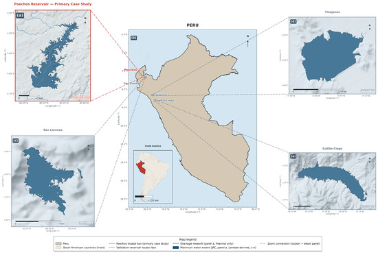
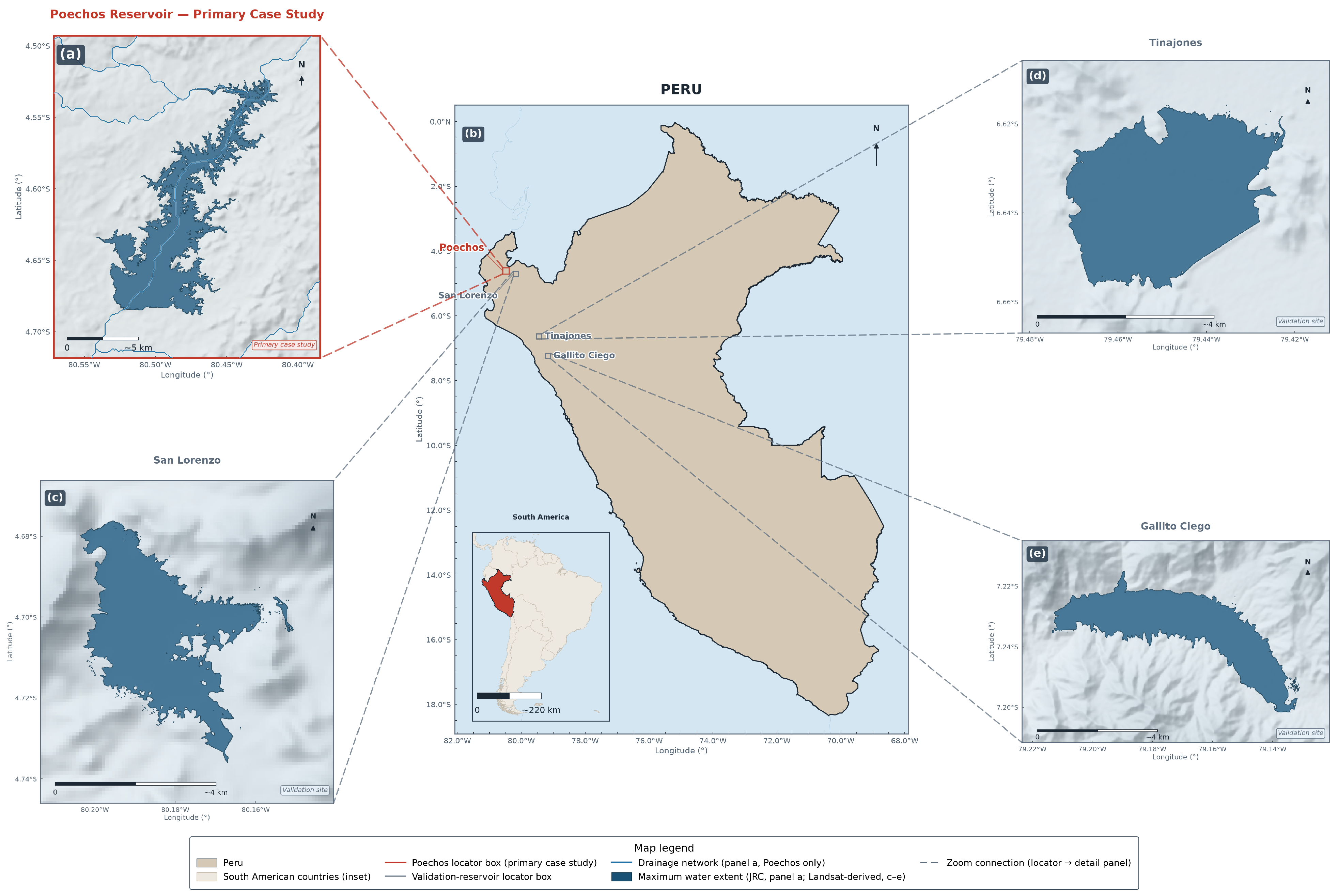
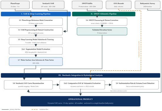
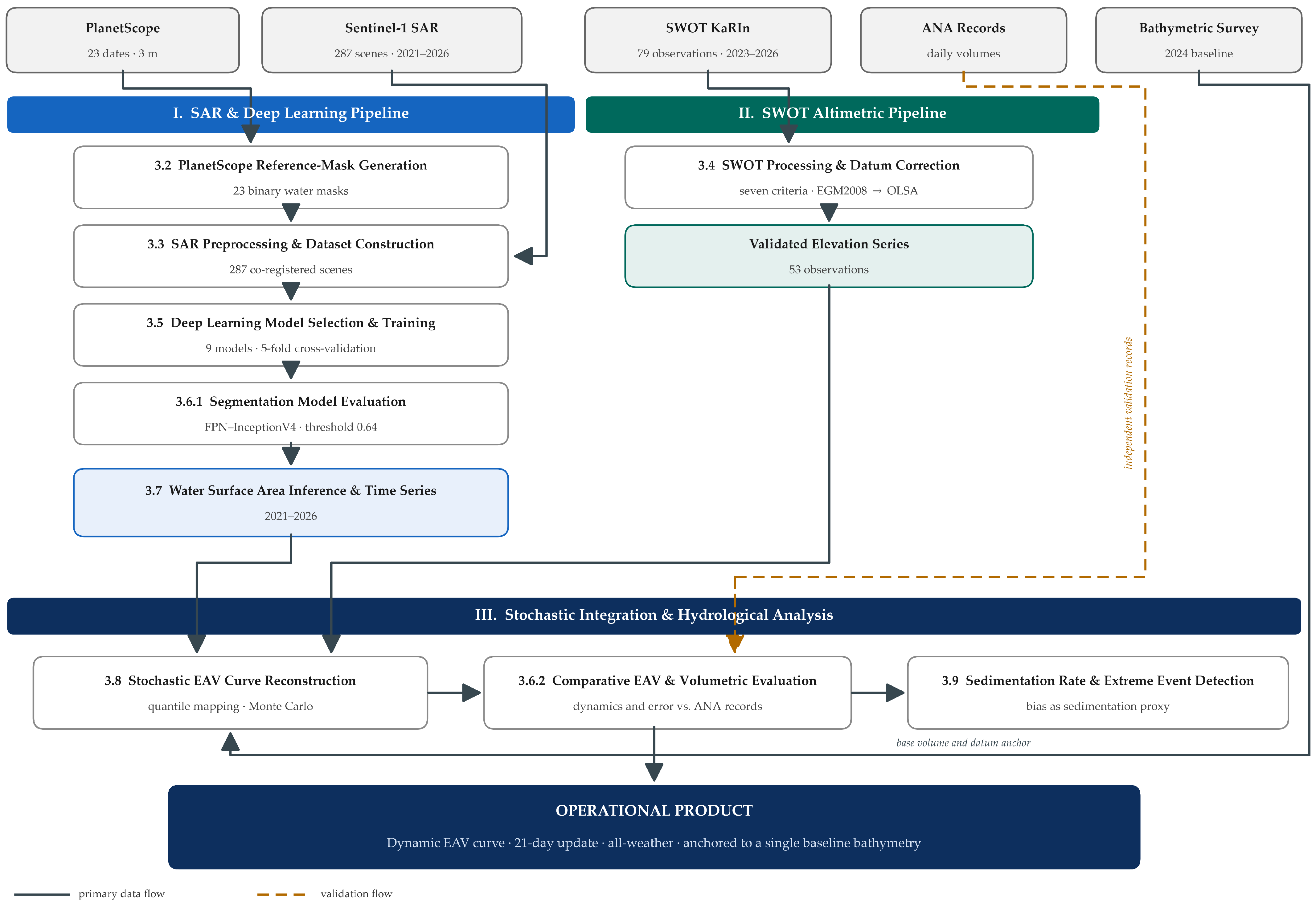
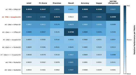
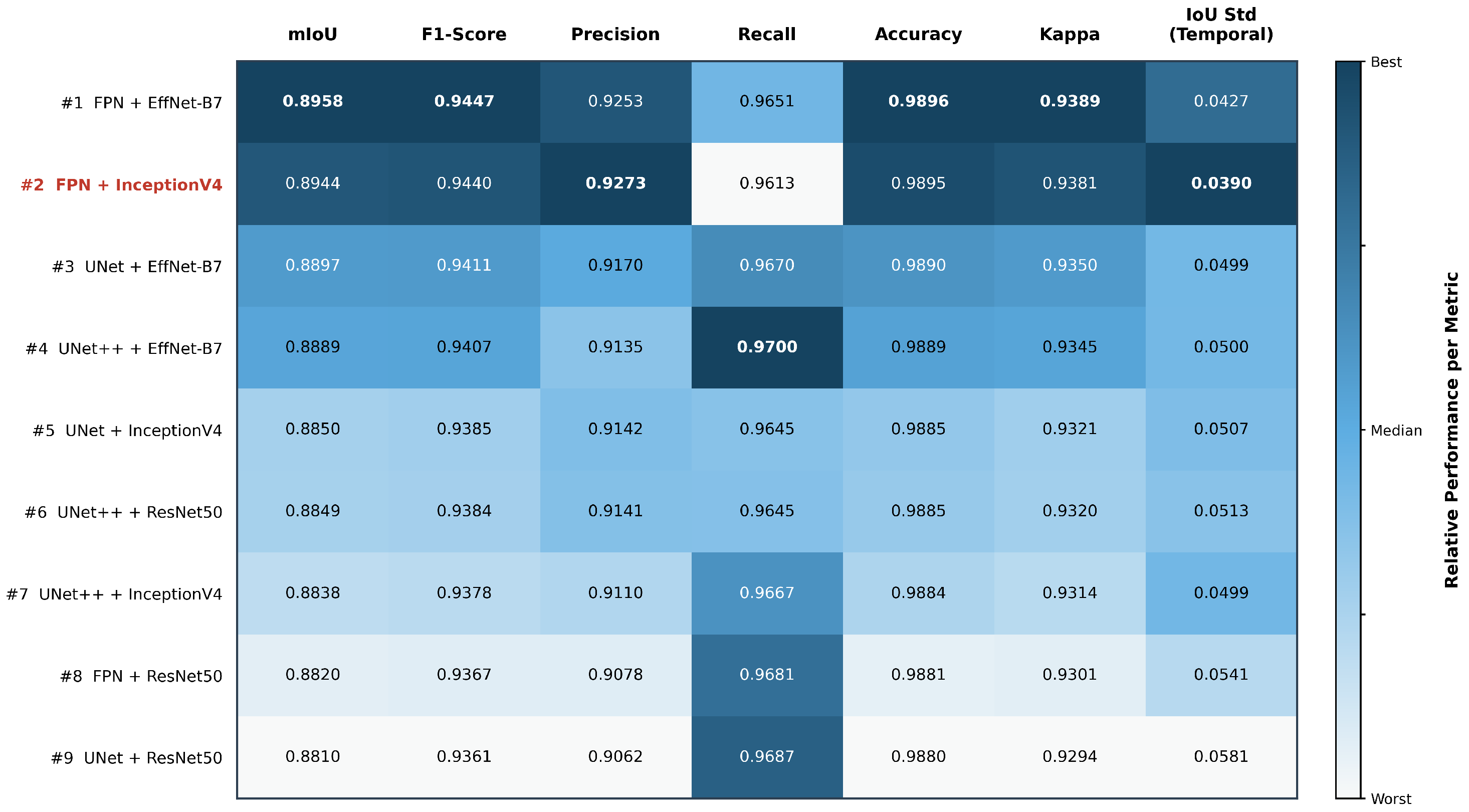
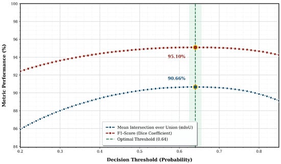
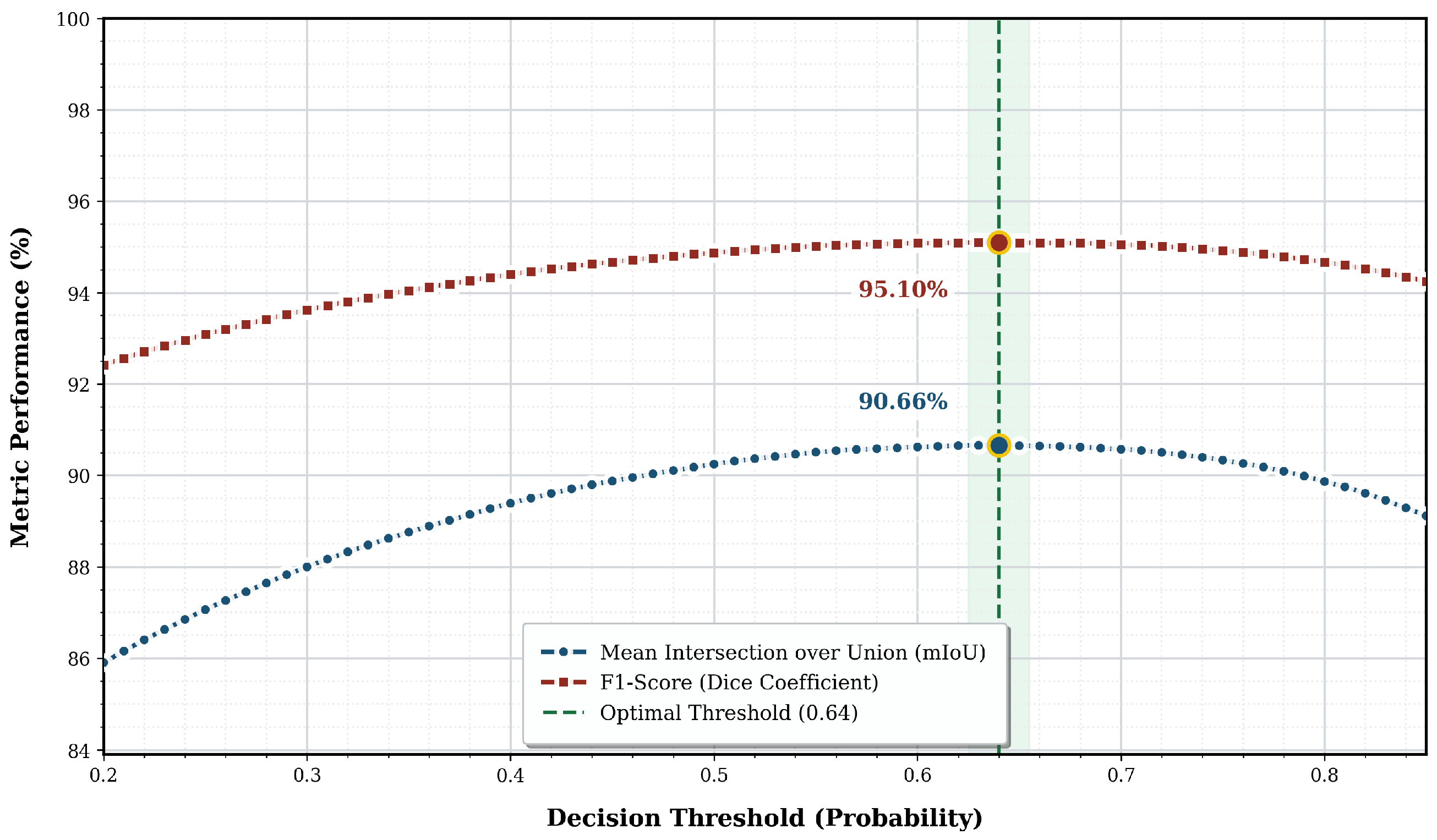
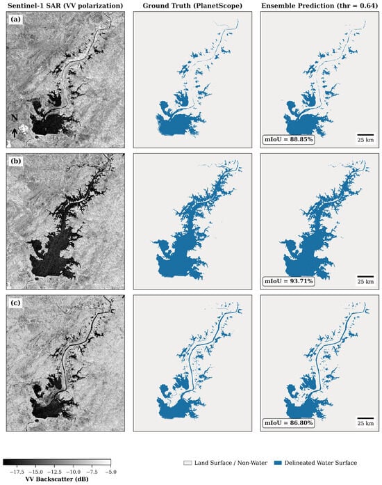
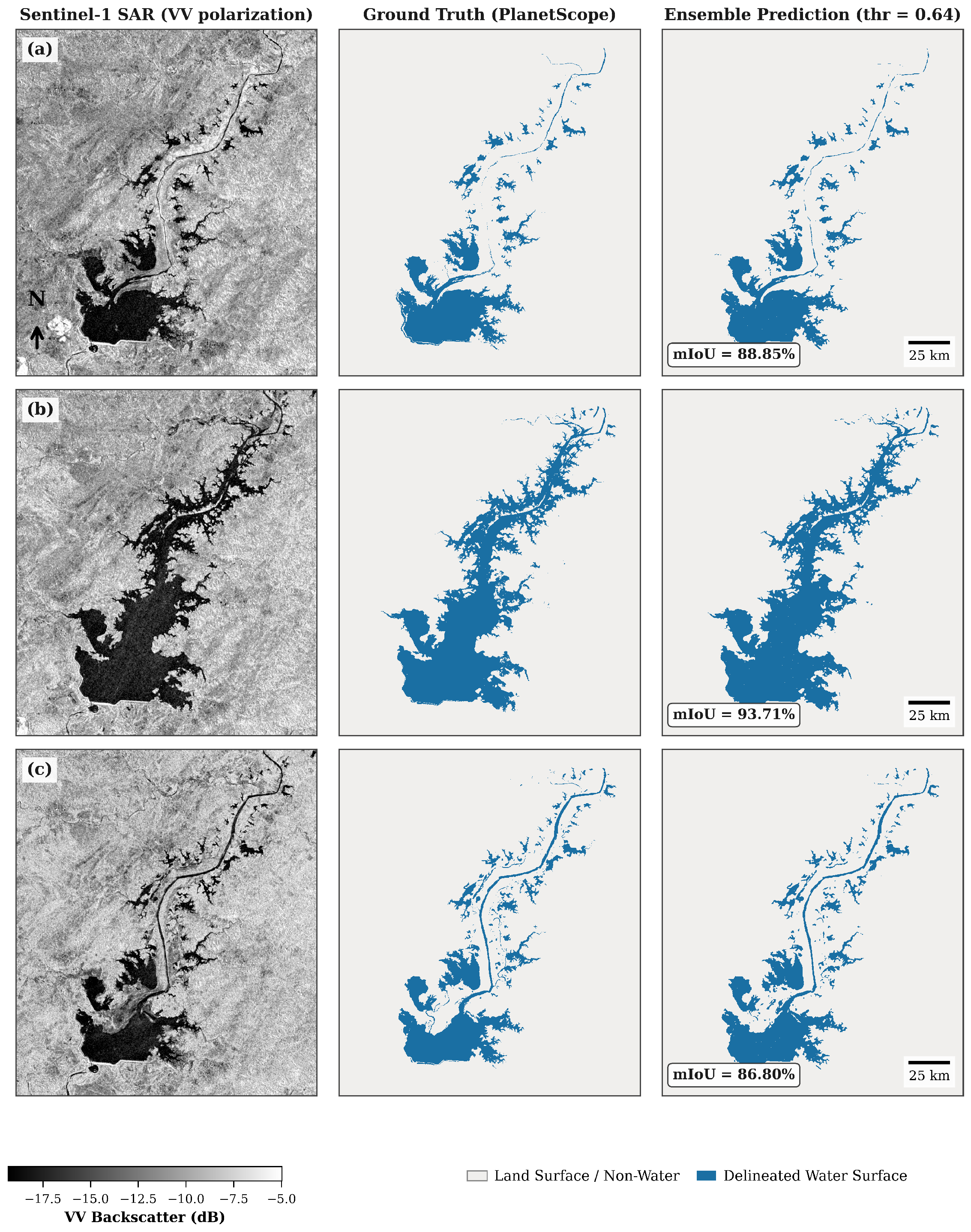
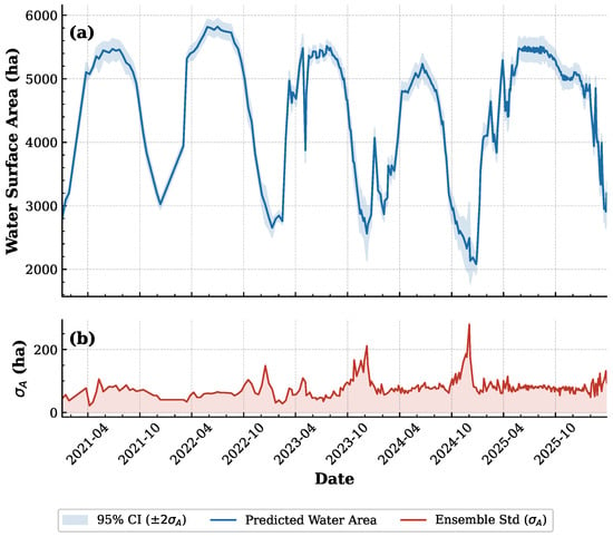
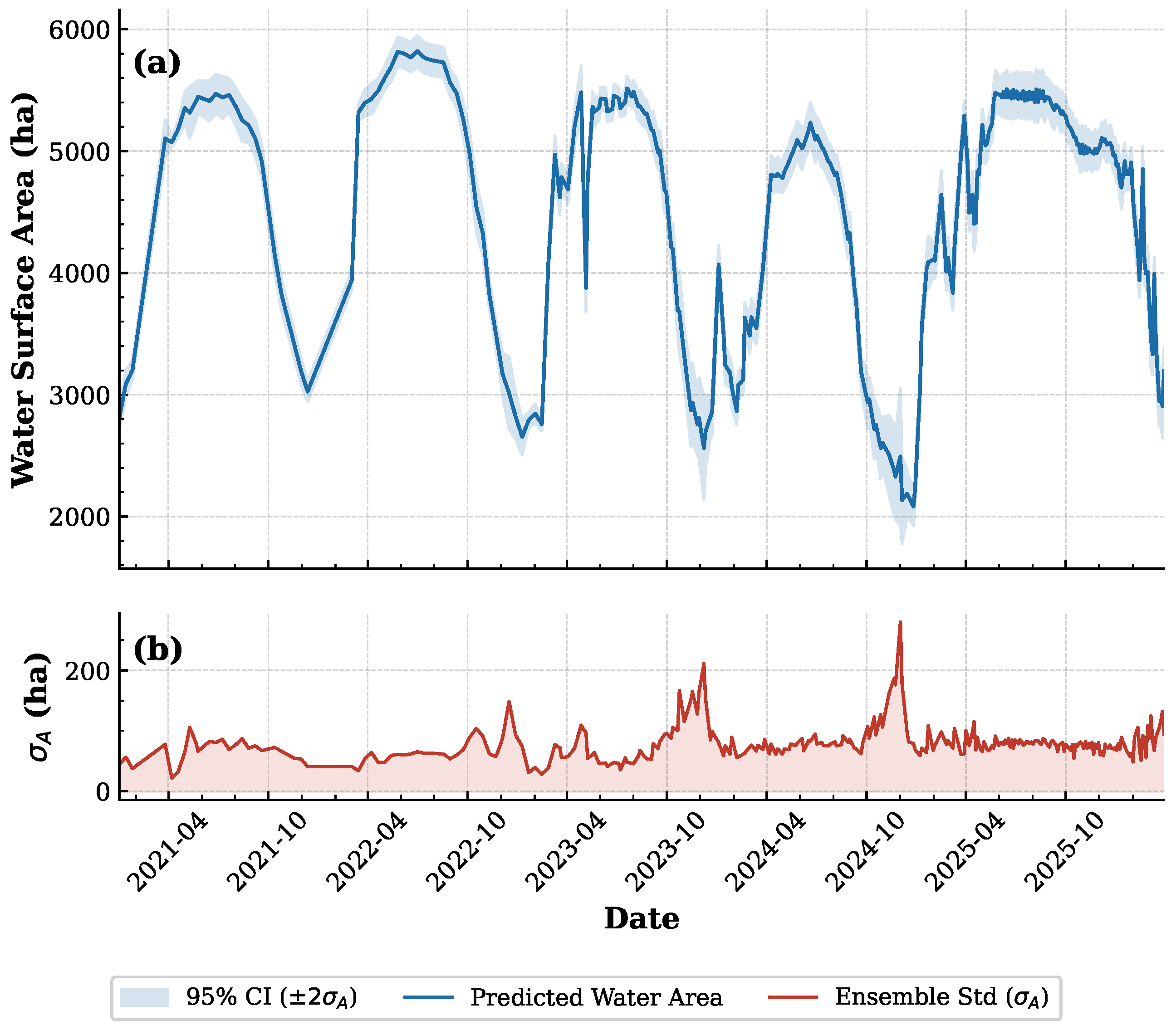
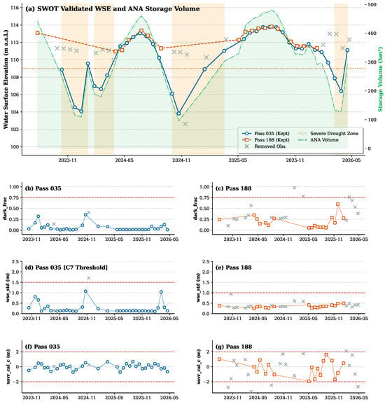
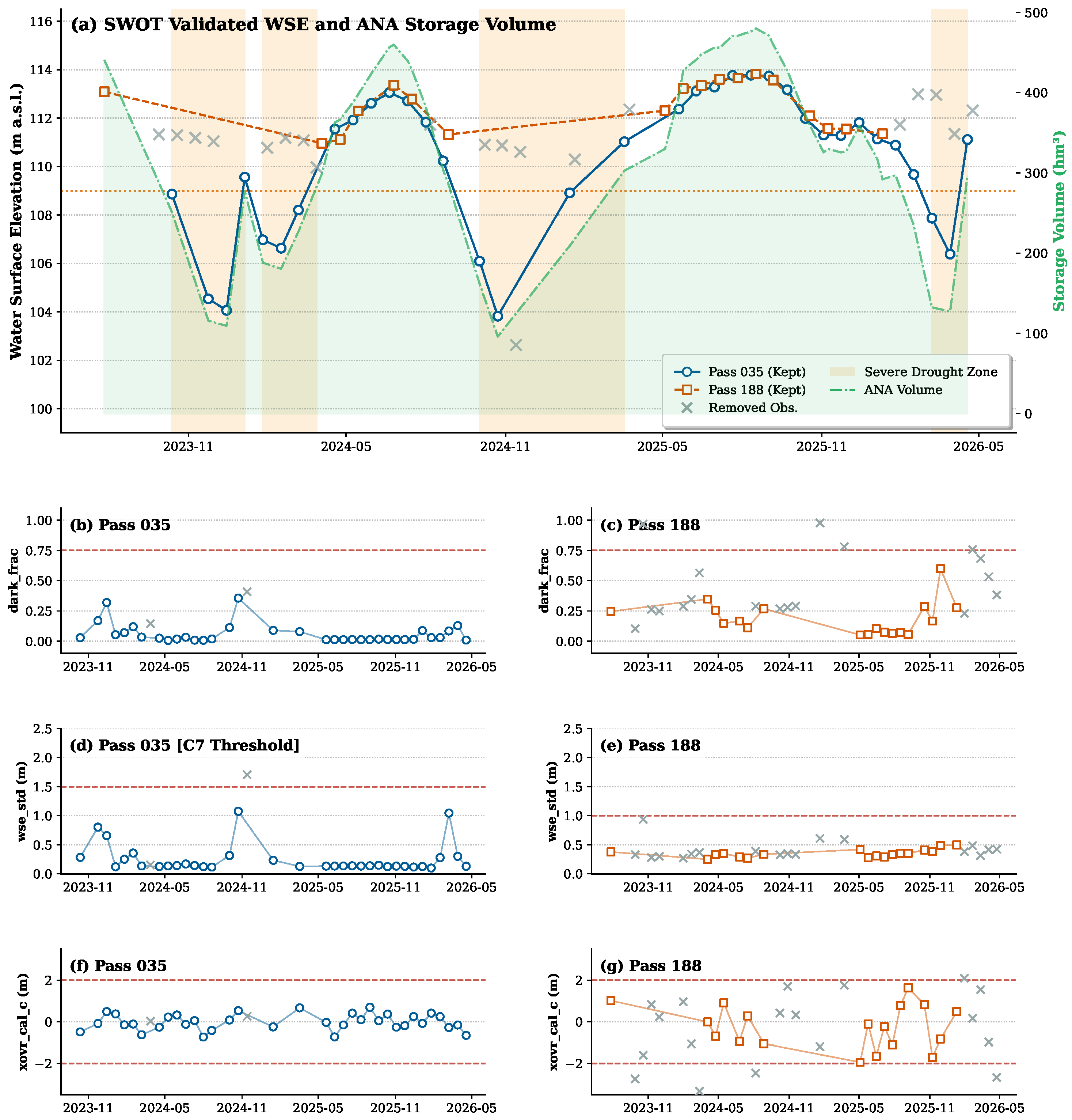
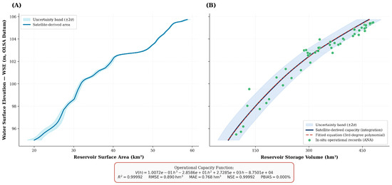
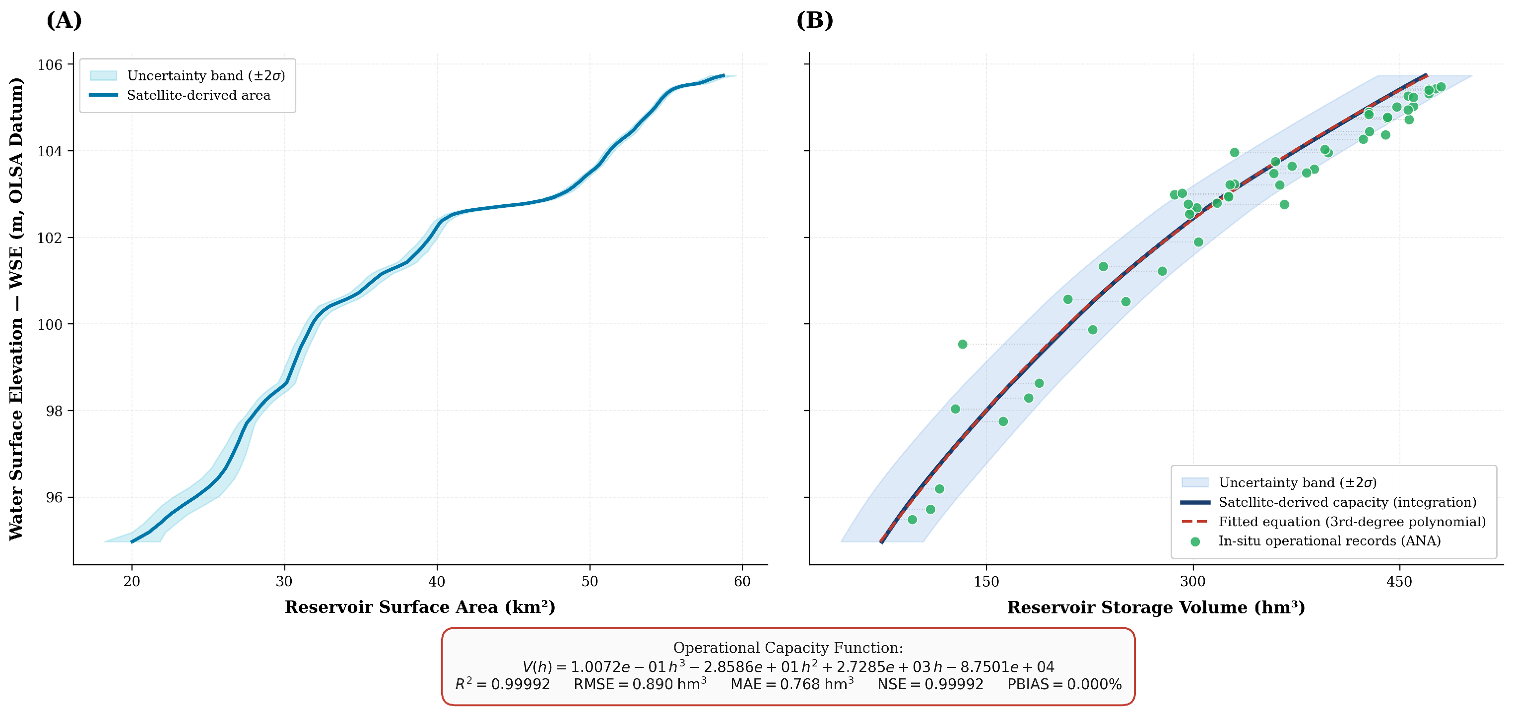
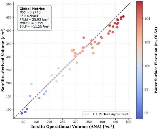
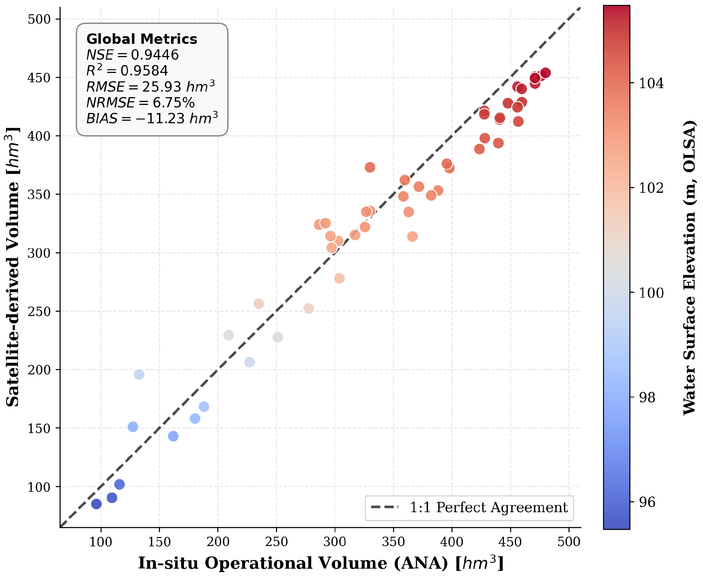
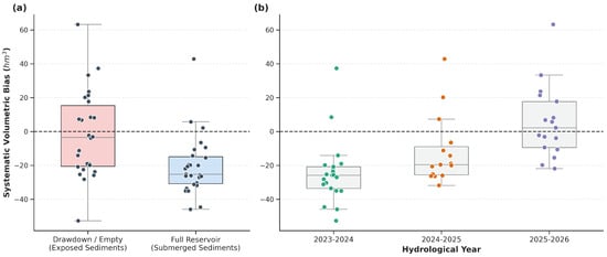
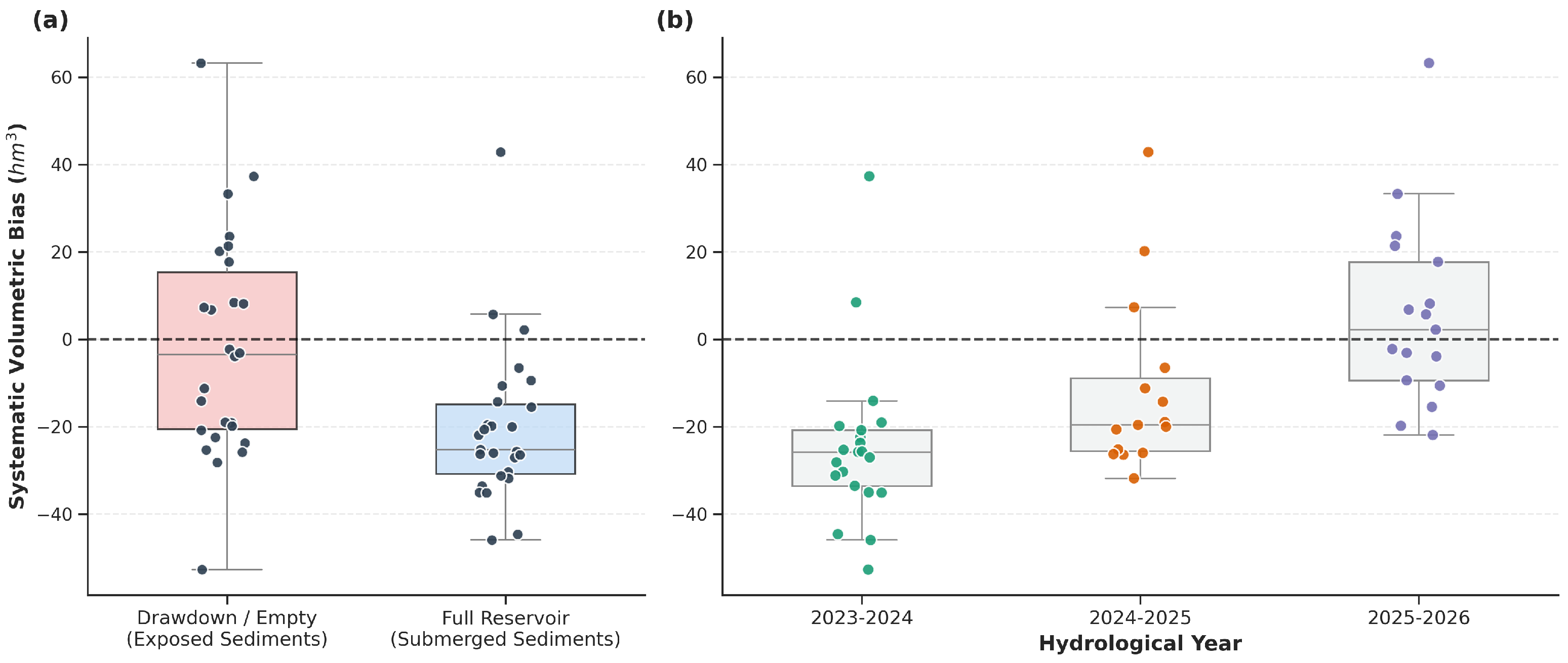
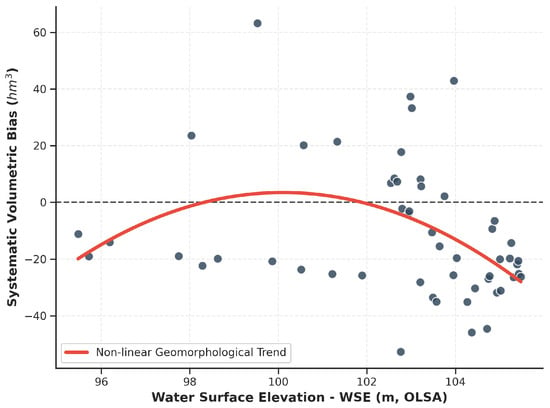
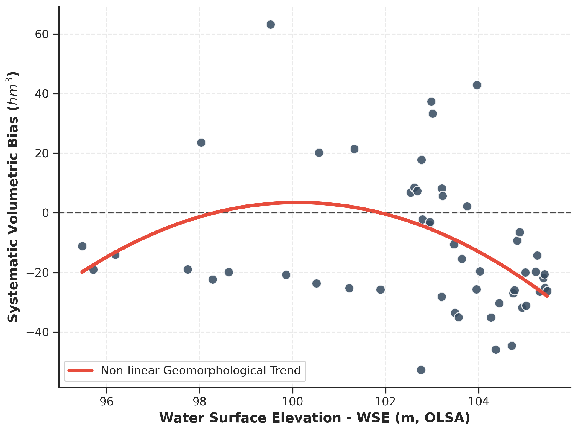
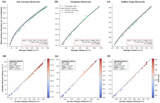
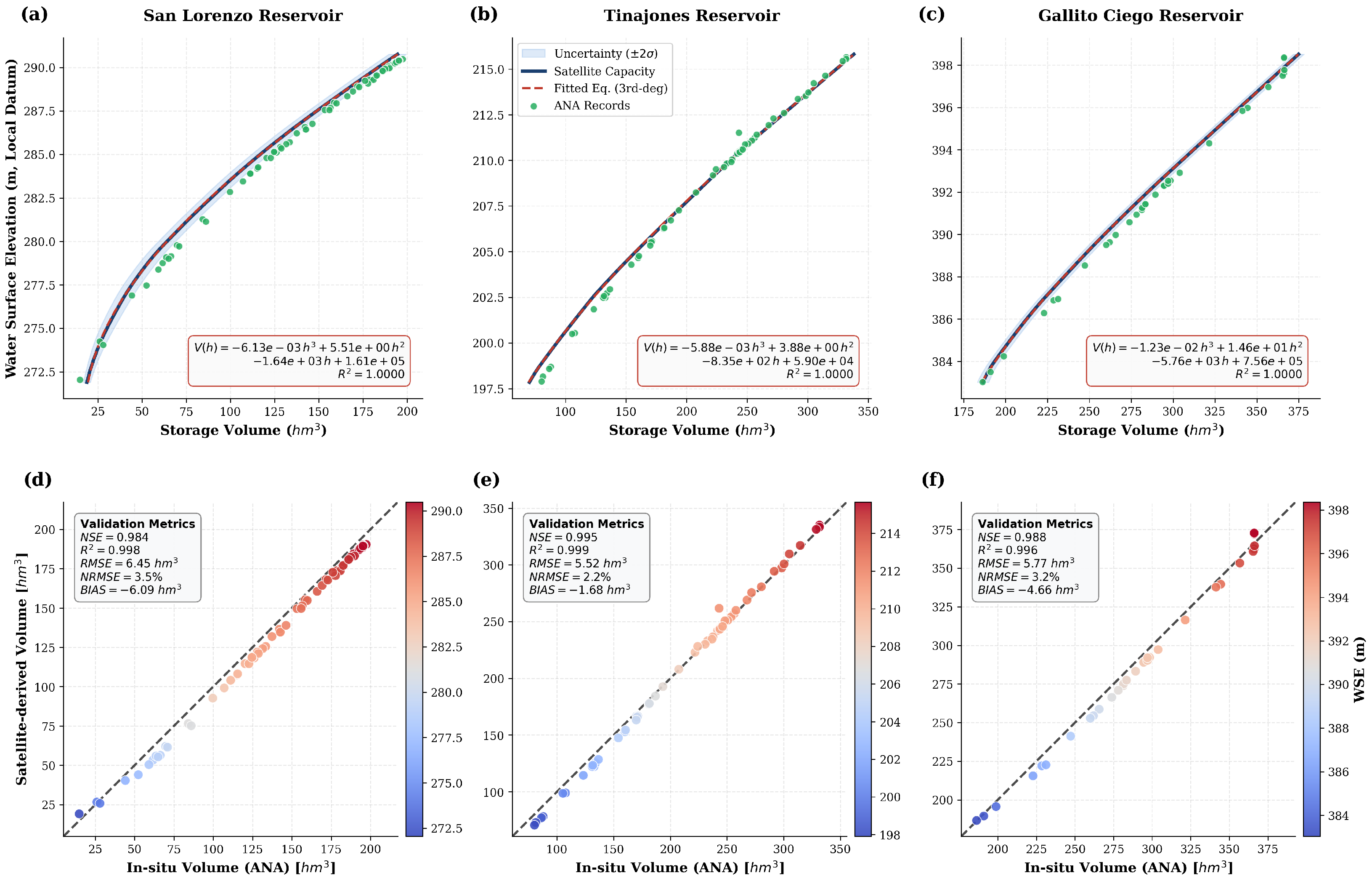
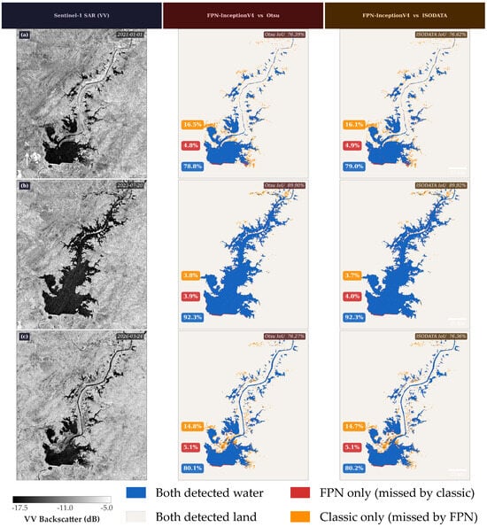
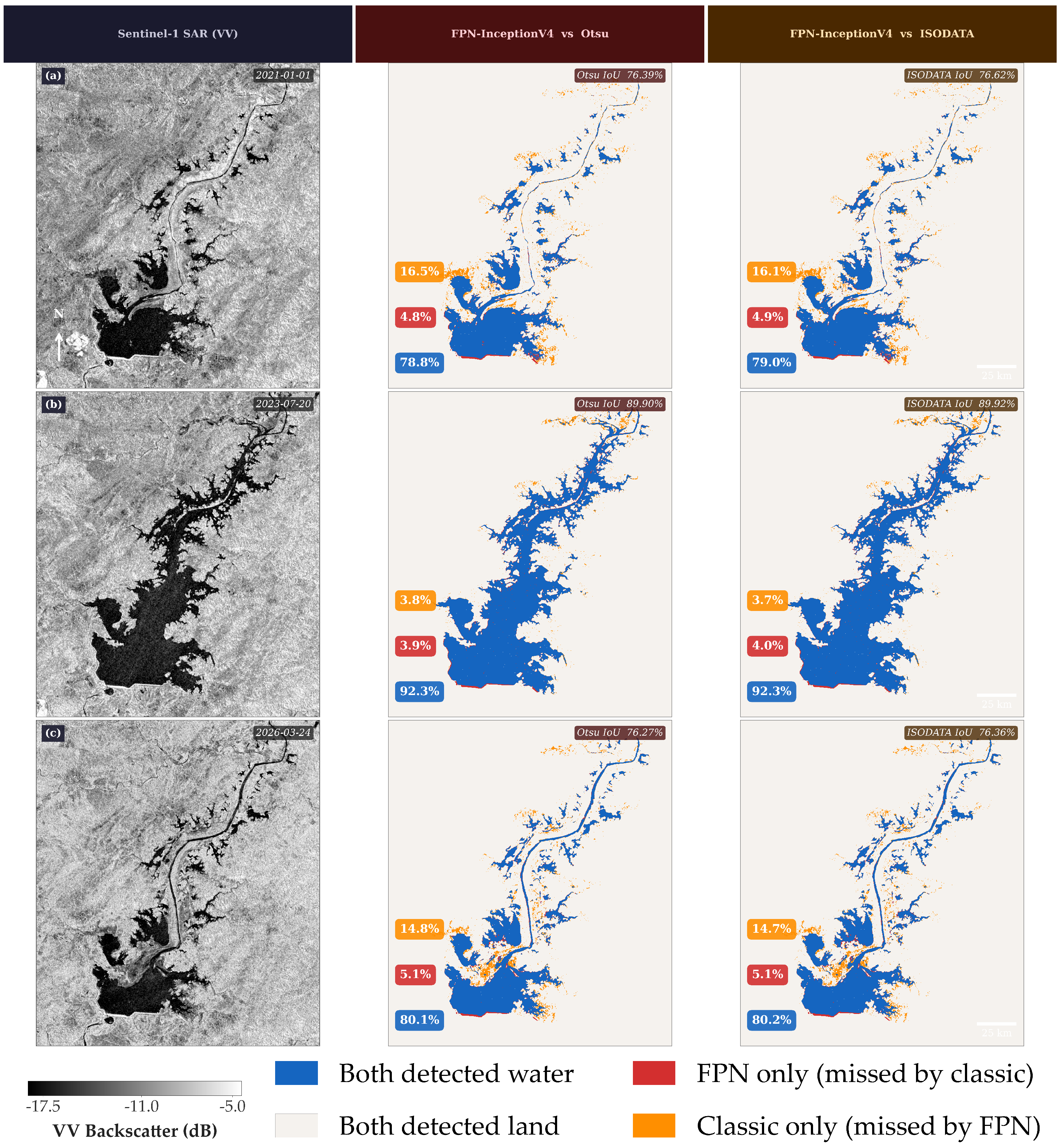
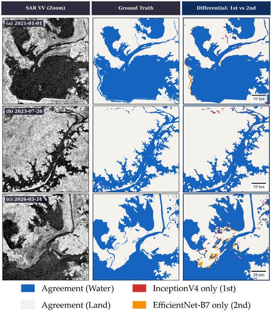
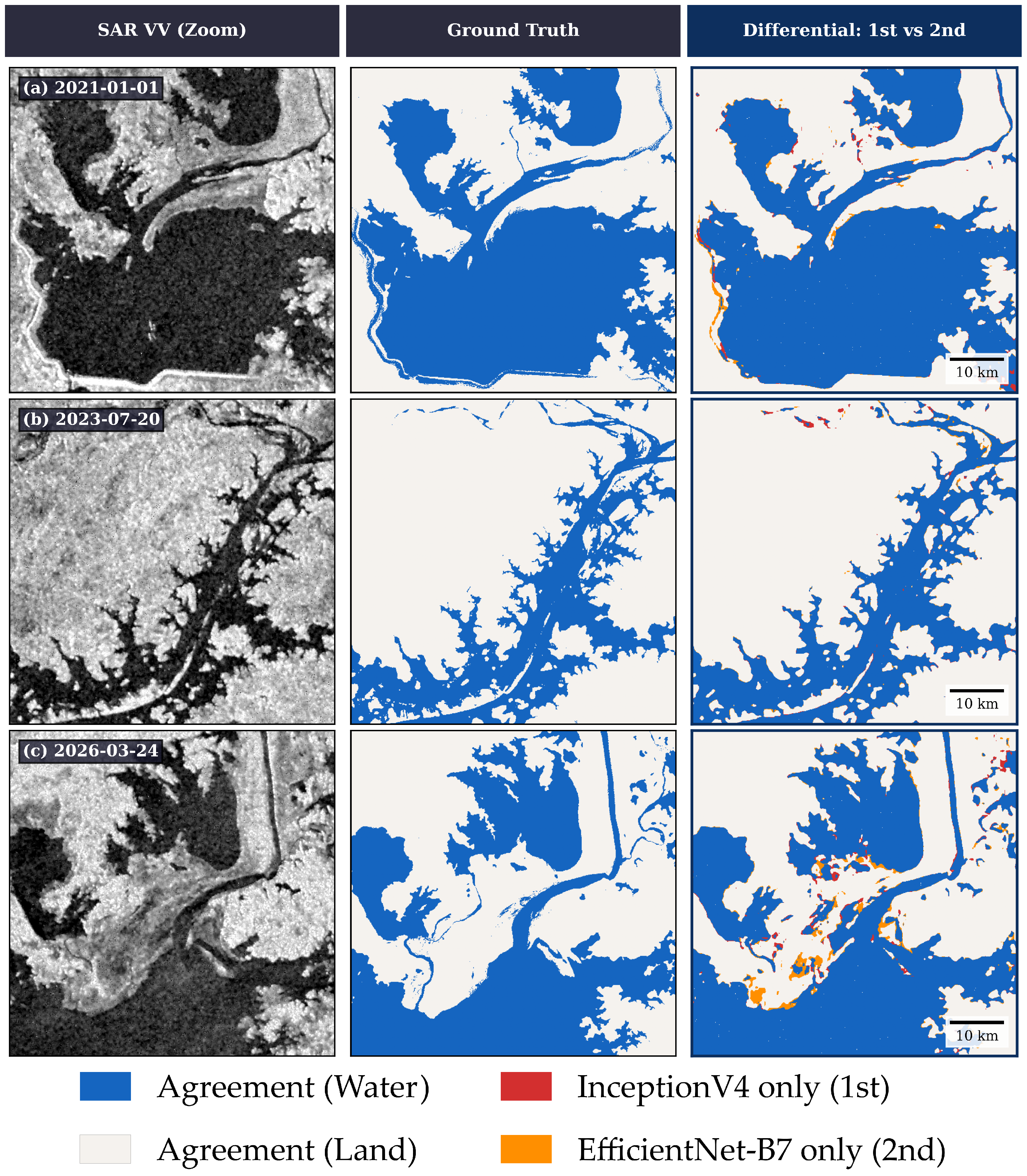

Disclaimer/Publisher’s Note: The statements, opinions and data contained in all publications are solely those of the individual author(s) and contributor(s) and not of MDPI and/or the editor(s). MDPI and/or the editor(s) disclaim responsibility for any injury to people or property resulting from any ideas, methods, instructions or products referred to in the content. |
© 2026 by the authors. Licensee MDPI, Basel, Switzerland. This article is an open access article distributed under the terms and conditions of the Creative Commons Attribution (CC BY) license.