Hybrid Cloud Segmentation Approach Combining YOLOv8 Instance Segmentation with HSV Thresholding for Multi-Site Assessment

Abstract

Accurate cloud segmentation from ground-based fisheye camera imagery is essential for solar irradiance forecasting and photovoltaic system optimization. Traditional computer vision approaches, such as HSV thresholding and K-means clustering, face significant limitations when applied globally to sky images due to the spectral similarity between cloud regions and sky areas under varying atmospheric conditions. This study presents a hybrid methodology that leverages YOLOv8 instance segmentation to provide contextual cloud regions followed by refined HSV thresholding within these detected areas. The approach incorporates solar trajectory modeling using pvlib for accurate sun disk detection and exclusion, preventing false cloud classification. The methodology was developed and validated at the CIESOL using Mobotix Q71 fisheye cameras, and later tested in Antofagasta (Chile) and Huelva (Spain). The YOLOv8l-seg model achieved a mask precision of 0.821 and box mAP@0.5 of 0.680 on validation data. The results show a promising correlation with radiometric measurements such as clearness index $k_t$ and diffuse fraction $k_d$ in preliminary validation cases. While YOLOv8 demonstrates good cross-site generalization, HSV thresholding requires camera-specific calibration for optimal performance. The method addresses the context-dependency limitations of traditional algorithms, though computational performance and broader validation remain areas for future work.

1. Introduction

Solar energy represents one of the most promising renewable energy sources for mitigating climate change and achieving sustainable energy systems [1]. However, the inherent variability in solar irradiance, primarily driven by cloud dynamics, poses significant challenges for photovoltaic system optimization, grid integration, and accurate power generation forecasting [2]. Cloud cover substantially affects surface solar irradiance, reducing the amount of incoming solar energy reaching the surface, particularly under stratocumulus and cumulonimbus conditions [3,4], making accurate cloud detection and characterization essential for operational solar energy systems.

Ground-based sky imaging systems, particularly those employing fisheye lenses, provide high temporal resolution observations suitable for short-term solar forecasting from minutes to hours ahead [5]. These systems complement satellite-based observations by offering localized, high-frequency measurements at specific installation sites. However, automated cloud segmentation from ground-based fisheye imagery remains a challenging computer vision problem due to several factors: the spectral similarity between thin clouds and clear sky regions, varying atmospheric conditions affecting color appearance, sun glare and bloom effects, and the need for robust performance across different geographical locations and camera systems.

Ground-based sky imaging systems using whole-sky imagers have become essential tools for cloud observation and solar energy applications. Long et al. [6] presented techniques for analyzing full-color sky images to infer cloud macrophysical properties, demonstrating that automated fractional sky cover retrievals show uncertainty comparable to human observations. Alonso-Montesinos et al. [7] developed sky camera imagery processing based on sky classifications using radiometric data, and in subsequent work [8,9] demonstrated solar irradiance forecasting at one-minute intervals using sky camera images and proposed methods for solar radiation estimation based on digital image processing. More recently, Alonso-Montesinos [10] presented an autonomous cloud detection system achieving a 94% success rate using Hue, Saturation, and Value (HSV) color space relationships without radiometric parameters, demonstrating the potential for real-time cloud identification from ground-based perspectives. However, this approach relies on global HSV thresholding, which faces limitations when spectral ambiguity occurs between thin clouds and clear sky regions under varying atmospheric conditions.

Traditional approaches to cloud segmentation have relied on color space transformations and clustering algorithms. Dev et al. [11] presented a supervised segmentation framework based on systematic analysis of different color spaces using Partial Least Squares regression, releasing the Singapore Whole-Sky IMaging SEGmentation Database. Their learning-based approach avoided manually defined parameters, addressing a key limitation of traditional thresholding methods. Escalona-Llaguno et al. [12] developed an automatic methodology based on artificial neural networks to discriminate between haze and cloudiness in the circumsolar region of all-sky camera images, achieving an overall classification accuracy of 84%. Chauvin et al. [13] developed an image processing methodology for cloud cover estimation to improve Direct Normal Irradiance forecasts at short-term horizons. Long et al. [6] noted that while automated sky imagers are useful for replacing traditional human observations, uncertainties remain in fractional sky cover retrievals, particularly for complex cloud scenarios.

Recent advances in deep learning have improved cloud segmentation performance. Yin et al. [14] proposed an improved U-Net architecture incorporating dilated convolution and Atrous Spatial Pyramid Pooling, achieving improvements of 2.2–5.0% over traditional U-Net on benchmark datasets. Li et al. [15] introduced BSANet, achieving real-time performance at 392 fps in Half-Precision Floating Point (FP16) precision through bilateral segregation and aggregation modules. Loddo et al. [16] conducted a comprehensive benchmark of seven semantic segmentation algorithms for cloud detection in remote sensing imagery from the Sentinel-2 and Landsat-8 satellites. Their analysis revealed that RS-Net and DeepLabV3+ consistently showed robust performance across datasets, with results highlighting the importance of algorithm selection tailored to specific dataset characteristics. They noted that future improvements could leverage ensemble methods, novel architectures, and integration of temporal patterns.

Related work in hyperspectral remote sensing further illustrates the broader value of combining data-driven representations with explicitly structured constraints. Huo et al. [17] used multi-scale memory and separation training to distinguish anomalies from the background in hyperspectral anomaly detection, whereas Qu et al. [18] incorporated graph regularization and sparsity constraints into deep non-negative matrix factorization for hyperspectral unmixing. While these methods operate on high-dimensional spectral data and target different remote sensing tasks, making them distinct from ground-based RGB cloud segmentation, they nevertheless motivate the general principle that learned representations can benefit from complementary structured priors; here, the corresponding priors are local HSV spectral criteria and solar geometry.

Zhu et al. [19] compared YOLO version 5 and 8 for cloud region recognition in remote sensing images, finding that YOLOv5-l achieved higher successful recognition rates, exceeding 95% with fewer missed detections, while YOLOv8 showed slightly better overall mean Average Precision. Their results indicate that performance varies significantly depending on dataset characteristics and evaluation priorities.

Hybrid strategies have previously combined multiple handcrafted thresholding rules, including the Hybrid Thresholding Algorithm (HYTA), which selects fixed or adaptive thresholds from image statistics [20]; comprehensive benchmarking has likewise compared threshold-based, hybrid, and fully convolutional cloud segmentation approaches [21]. However, such threshold-based hybrid approaches still make the cloud–sky decision from image-derived spectral criteria alone. The methodological novelty of the present work is not the mere combination of learning and thresholding, but the conditional use of a handcrafted spectral rule after learned instance-level contextual recognition. YOLOv8 first provides cloud-support regions that encode spatial extent, texture, morphology, and neighborhood information; HSV thresholding is subsequently used only within those regions to refine the pixel-level boundary. Consequently, pixels with the same HSV values are not classified globally, but according to whether they occur inside a region that the CNN has identified as cloud-like. The approach is further constrained by an astronomically informed solar-exclusion stage, which removes a major source of brightness-related false positives.

This methodology was developed to function reliably across multiple geographical sites while maintaining computational efficiency for real-time applications. An important design principle was to achieve robust cloud segmentation using affordable, commercially available hardware—specifically the Mobotix Q71 fisheye camera system—rather than requiring expensive high-end equipment. While this camera family presents limitations in spatial resolution and dynamic range, the proposed context-gated framework successfully overcomes these hardware constraints, making the methodology accessible for broader deployment.

The main contributions of this work are: (i) a context-gated cloud segmentation framework in which YOLOv8 instance masks constrain HSV-based boundary refinement; (ii) a sun exclusion procedure that combines pvlib solar position calculations, fisheye projection calibration, and image-based validation; (iii) an analysis of cross-site behavior that distinguishes the transferability of CNN-based recognition from the camera dependence of static HSV thresholds; and (iv) a preliminary radiometric consistency assessment using the clearness index and diffuse fraction.

To assess its multi-site applicability and generalization capability, the system was developed and validated at the CIESOL center (36.8305°N, 2.4071°W), with subsequent testing at the University of Antofagasta (23.6692°S, 70.4056°W) and the University of Huelva (37.20°N, 6.9202°W).

The remainder of this paper is organized as follows: Section 2 describes the materials and methods, including sun detection, traditional approaches, and the hybrid integration framework; Section 3 presents the experimental results along with the multi-site and radiometric validation; and Section 4 discusses the core findings and limitations, and concludes with future work directions.

2. Materials and Methods

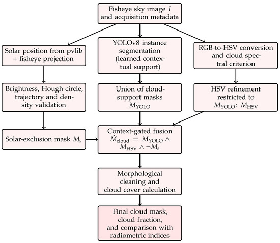
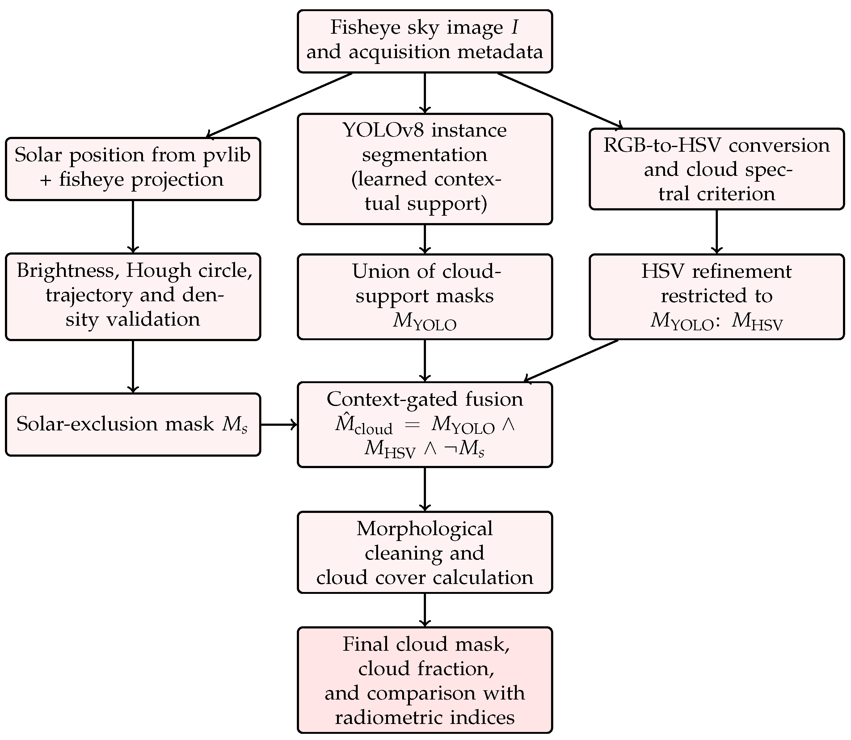
The hybrid cloud segmentation methodology consists of three main stages: sun detection and exclusion using solar trajectory modeling, contextual cloud region detection using YOLOv8 instance segmentation, and refined cloud boundary delineation using HSV thresholding within detected regions. Figure 1 shows an overall workflow with the most important steps that are describing more detailed in this section.

Figure 1. Overall workflow of the proposed context-gated hybrid cloud segmentation pipeline. YOLOv8 supplies learned cloud-support regions, HSV supplies local spectral refinement, and the pvlib-based branch excludes the solar region before the final cloud mask and cloud fraction are calculated.

The development and training were conducted on a workstation with a Windows 11 operating system, Python version 3.11.11, NVIDIA GeForce RTX 4070 Ti graphics processing unit with 12 GB of video memory, PyTorch version 2.3.1 with CUDA 11.8 support, and cuDNN version 8700. More extensive studies employing larger models and datasets would benefit from higher-end computational resources.

2.1. Solar Trajectory Modeling and Sun Detection

Accurate sun detection and exclusion is critical for cloud segmentation, as the sun disk exhibits maximum brightness, V = 255 in HSV color space, which is similar to highly reflective cloud regions, leading to potential misclassification. Previous approaches to sun detection in sky camera imagery have employed different strategies. Alonso et al. [22] developed a methodology based on radiometric data to determine the sun area and identify cloud presence in saturated zones with a 92% success rate. In contrast, Alonso-Montesinos [10] achieved a 94% success rate using purely image-based HSV color space relationships without radiometric parameters. In this work, a mathematical approach combining astronomical calculations with image processing is employed to reliably detect and mask the sun, providing a robust alternative that leverages both astronomical precision and computer vision techniques.

2.1.1. Solar Position Calculation

The pvlib-python library [23], a comprehensive toolkit for simulating photovoltaic system performance, is utilized to calculate solar positions. The library implements the NREL Solar Position Algorithm [24], which provides solar zenith and azimuth angles with uncertainty below 0.0003°.

Given a timestamp t, geographical coordinates (latitude $\varphi$, longitude $\lambda$), and altitude above sea level h, pvlib computes:

$$\begin{array}{cc}\hfill {\theta }_z\left(t\right)& =\arccos (\sin \varphi \sin \delta +\cos \varphi \cos \delta \cos \omega )\hfill \\ \hfill {\gamma }_s\left(t\right)& =\arctan 2(-\sin \omega \cos \delta ,\sin \delta \cos \varphi -\cos \delta \sin \varphi \cos \omega )\hfill \end{array}$$

(1)

where ${\theta }_z$ is the solar zenith angle, ${\gamma }_s$ is the solar azimuth angle, $\delta$ is the solar declination, $\omega$ is the hour angle, and $\arctan 2(y,x)$ is the two-argument arctangent function that returns the angle in the correct quadrant.

For the CIESOL installation, the geographical coordinates used are $\varphi =36.8305°$N, $\lambda =2.4071°$W, and $h=0$ m, as the facility is located at sea level.

2.1.2. Coordinate Transformation

The calculated solar positions, including zenith and azimuth angles, must be transformed to image pixel coordinates accounting for the fisheye lens projection. A radial projection model is employed where the radial distance from the image center is proportional to the zenith angle:

$$\begin{array}{cc}\hfill r& ={\displaystyle \frac{{\theta }_z}{\pi /2}}·R_{\mathrm{fisheye}}·f_{\mathrm{scale}}\hfill \\ \hfill x_{\mathrm{rel}}& =r\cos ({\gamma }_s+{\alpha }_{\mathrm{offset}})\hfill \\ \hfill y_{\mathrm{rel}}& =r\sin ({\gamma }_s+{\alpha }_{\mathrm{offset}})\hfill \end{array}$$

(2)

where ${\theta }_z$ is the solar zenith angle, ${\gamma }_s$ is the solar azimuth angle, $R_{\mathrm{fisheye}}$ is the fisheye radius in pixels (distance from center to image edge), $f_{\mathrm{scale}}=1.5$ is an empirically determined distortion factor that adjusts the radial mapping, and ${\alpha }_{\mathrm{offset}}$ = 90° accounts for camera rotation relative to North.

These parameters were calibrated by comparing predicted sun positions from pvlib with observed sun positions in actual fisheye images across different times and dates, ensuring that the solar trajectory fit properly within the camera’s field of view. Additional corrections are applied to account for camera mounting:

$$\left(\begin{array}{c}{x}_{\mathrm{img}}\\ y_{\mathrm{img}}\end{array}\right)=\left(\begin{array}{c}{x}_c\\ y_c\end{array}\right)+\left(\begin{array}{c}{I}_x·x_{\mathrm{rel}}+\mathrm{\Delta }x\\ I_y·y_{\mathrm{rel}}+\mathrm{\Delta }y\end{array}\right)$$

(3)

where $(x_c,y_c)$ is the image center; $I_x,I_y\in \{-1,1\}$ are axis inversion flags for horizontal and vertical flipping; and $(\mathrm{\Delta }x,\mathrm{\Delta }y)$ are pixel offsets with $\mathrm{\Delta }x=20$ px and $\mathrm{\Delta }y=-60$ px for the CIESOL installation that compensate for slight camera misalignment.

2.1.3. Sun Detection Algorithm

The sun detection algorithm operates in multiple stages. Before applying the detection pipeline, the input image undergoes preprocessing to enhance contrast and reduce noise.

Stage 0: Image Preprocessing

To improve the robustness of sun detection under varying atmospheric conditions, two preprocessing steps are applied:

• Contrast-Limited Adaptive Histogram Equalization (CLAHE): This technique divides the image into small regions and applies histogram equalization to each one separately, but with a limitation on contrast amplification to prevent excessive noise enhancement. It is specifically applied to the luminance channel (Value in HSV) to improve the visibility of the solar disk even when it is partially obscured by thin clouds or haze. The contrast limitation is key because it enhances details without creating visual artifacts.
• Bilateral Filtering: This filter works intelligently by considering both spatial proximity and intensity similarity between pixels. Unlike other smoothing filters, it preserves sharp edges while removing high-frequency noise. In the context of sun detection, it is especially valuable for eliminating small lens flares, defective sensor pixels that appear as anomalous bright spots, and other artifacts that could be mistaken for the solar disk during circle processing.

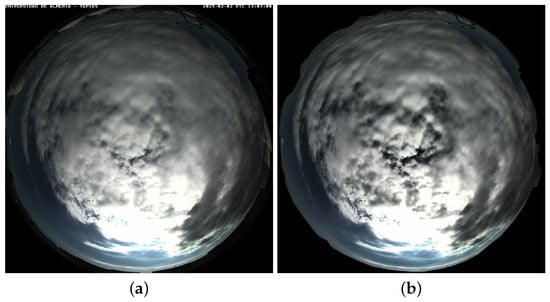
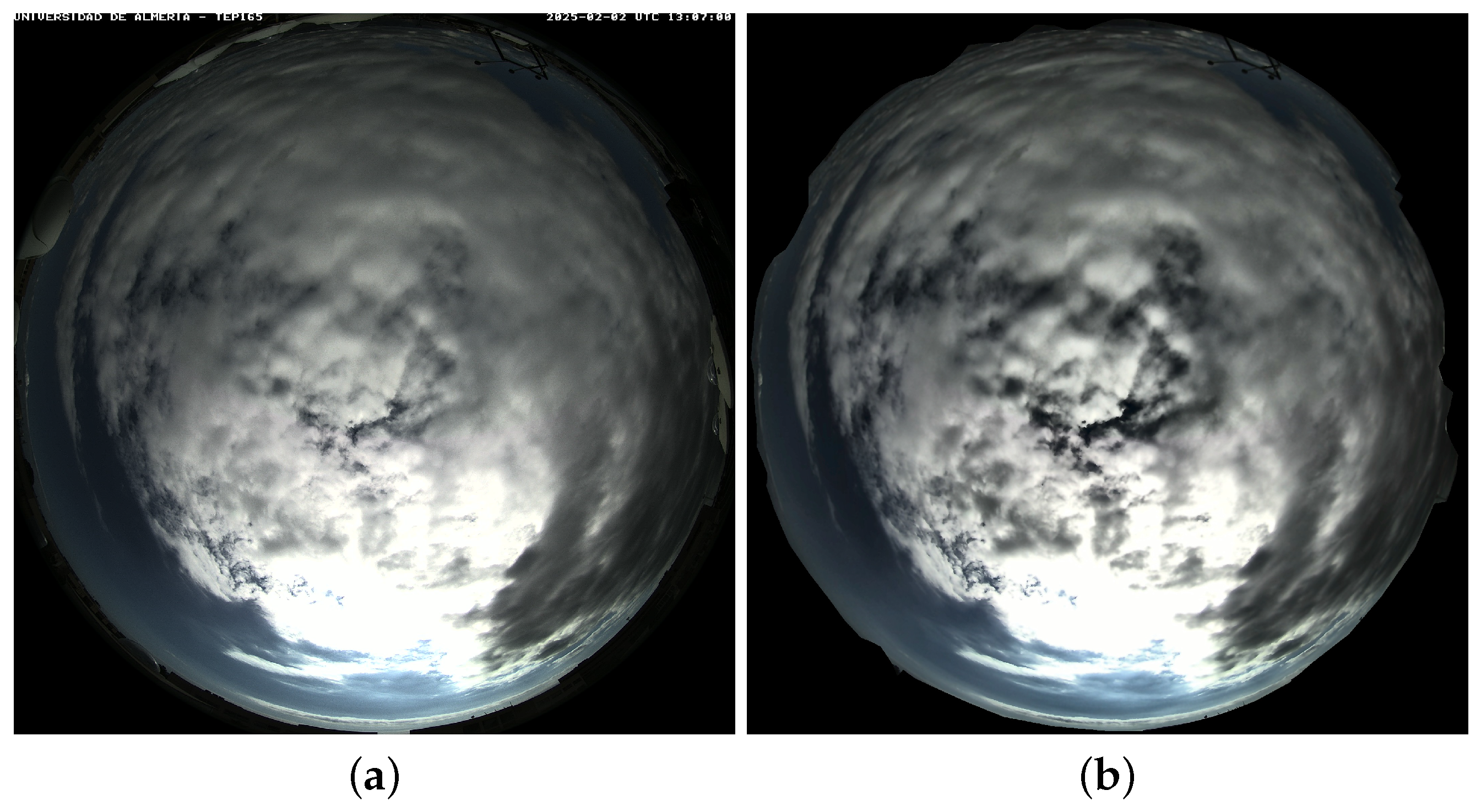
The goal of these preprocessing steps is to maximize the visual information available in the image before further analysis, minimizing discrepancies that may arise between ideal and real-world capture conditions. By enhancing details and removing artifacts, the detection model is provided with a more consistent and reliable data basis for processing. As shown in Figure 2, although these improvements may not be fully perceptible to the human eye, they are crucial for digital processing algorithms, which can detect and leverage these subtle enhancements in contrast and noise reduction.

Figure 2. Comparison of image preprocessing effects: (a) original image and (b) image after applying CLAHE and bilateral filtering.

Stage 1: Brightness Masking

Extract the V (Value) channel from the preprocessed HSV image and create a binary mask of maximum brightness pixels:

$$M_{\mathrm{bright}}(x,y)=\left\{\begin{array}{cc}255\hfill & \mathrm{if}V(x,y)=255\hfill \\ 0\hfill & \mathrm{otherwise}\hfill \end{array}\right.$$

(4)

Stage 2: Early Rejection

Count the total number of maximum brightness pixels: $N_{\mathrm{bright}}={\sum }_{x,y}⊮[M_{\mathrm{bright}}(x,y)=255]$. The sun must present a minimum number of bright pixels to be detectable, so if $N_{\mathrm{bright}}<N_{\min }$, the image is discarded as the sun is likely occluded by clouds. Here, the minimum area threshold is not a fixed value, but is dynamically set as $N_{\min }=\pi r_{\min }^2$, where $r_{\min }$ is the minimum expected radius of the sun in pixels. This ensures that the threshold adapts to the image scale and detection parameters. If the number of bright pixels exceeds this threshold, it may correspond to the sun or to bright clouds, but distinguishing between these cases requires the more advanced detection operations of the subsequent stages.

Stage 3: Morphological Filtering

Apply a morphological opening using an elliptical kernel of size $15\times 15$ pixels, with the aim of removing small bright spots present in the image. In this way, possible noise in the mask is reduced; that is, isolated or scattered pixels that could affect the final segmentation are eliminated:

$$M_{\mathrm{processed}}=(M_{\mathrm{bright}}\ominus K_{\mathrm{ellipse}})\oplus K_{\mathrm{ellipse}}$$

(5)

where ⊖ and ⊕ denote erosion and dilation operations, and $K_{\mathrm{ellipse}}$ is the elliptical structuring element.

Stage 4: Hough Circle Detection

The Hough Circle Transform [25] analyzes the processed image to identify circular patterns that could correspond to the solar disk. This technique works by accumulating votes in a three-dimensional parameter space $(x,y,r)$, where each point in the image votes for all possible circles that could pass through it. The circles with the highest number of votes are considered valid candidates.

$$HoughCircles(M_{\mathrm{processed}},d_{\min },r_{\min },r_{\max },p_2)$$

(6)

The parameters used are: minimum distance between centers $d_{\min }=h/4$ (where h is the image height), radius range of $r_{\min }=70$ pixels to $r_{\max }=230$ pixels (based on the typical size of the sun in fisheye camera images), and accumulator threshold $p_2=5$ (controls detection sensitivity). This stage generates a list of circular candidates that will later be validated by pixel density analysis and proximity to the expected solar trajectory.

Stage 5: Trajectory Validation

For each detected circle $(x_i,y_i,r_i)$, calculate the expected sun position $(x_{\mathrm{sun}},y_{\mathrm{sun}})$ from pvlib for the image timestamp and compute the Euclidean distance in pixel coordinates:

$$d_i=\sqrt{{(x_i-x_{\mathrm{sun}})}^2+{(y_i-y_{\mathrm{sun}})}^2}$$

(7)

Accept the circle as a valid sun detection if $d_i<d_{\mathrm{tol}}=150$ pixels. This tolerance accounts for potential inaccuracies in the fisheye projection model, camera calibration uncertainties, and atmospheric refraction effects.

Stage 6: Density Validation

For validated candidates, compute pixel density within the circle:

$${\rho }_i={\displaystyle \frac{{\sum }_{(x,y)\in C_i}⊮[V(x,y)=255]}{\pi r_i^2}}$$

(8)

where $C_i$ is the set of pixels within circle i. Accept the sun if ${\rho }_i>{\rho }_{\min }=0.85$.

Stage 7: Sun Mask Creation

For the best validated candidate (highest density), an exclusion mask is created with an expanded radius $r_{\mathrm{mask}}=1.15\times r_{\mathrm{detected}}$ to account for solar bloom effects. The bloom effect is an optical phenomenon that occurs when the sun saturates the sensor pixels, creating a saturation halo that extends beyond the actual solar disk. This halo can interfere with the detection of clouds near the sun, so an adaptive gamma correction is applied that reduces the brightness of pixels closest to the sun while maintaining the normal brightness of distant pixels.

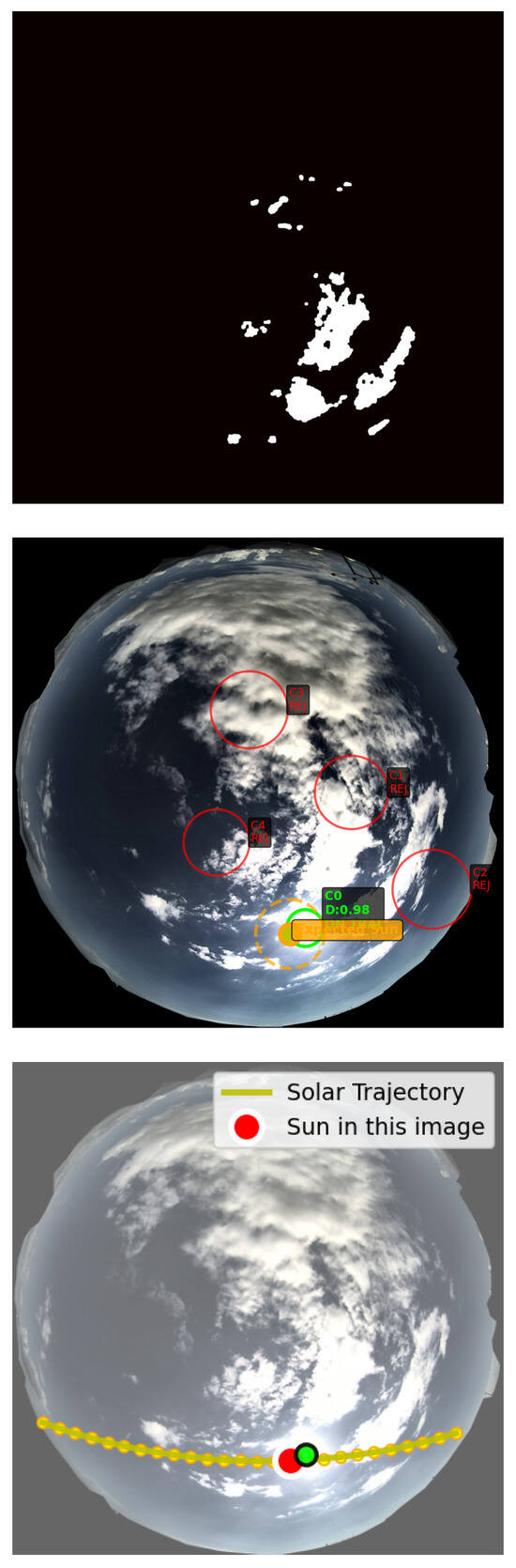
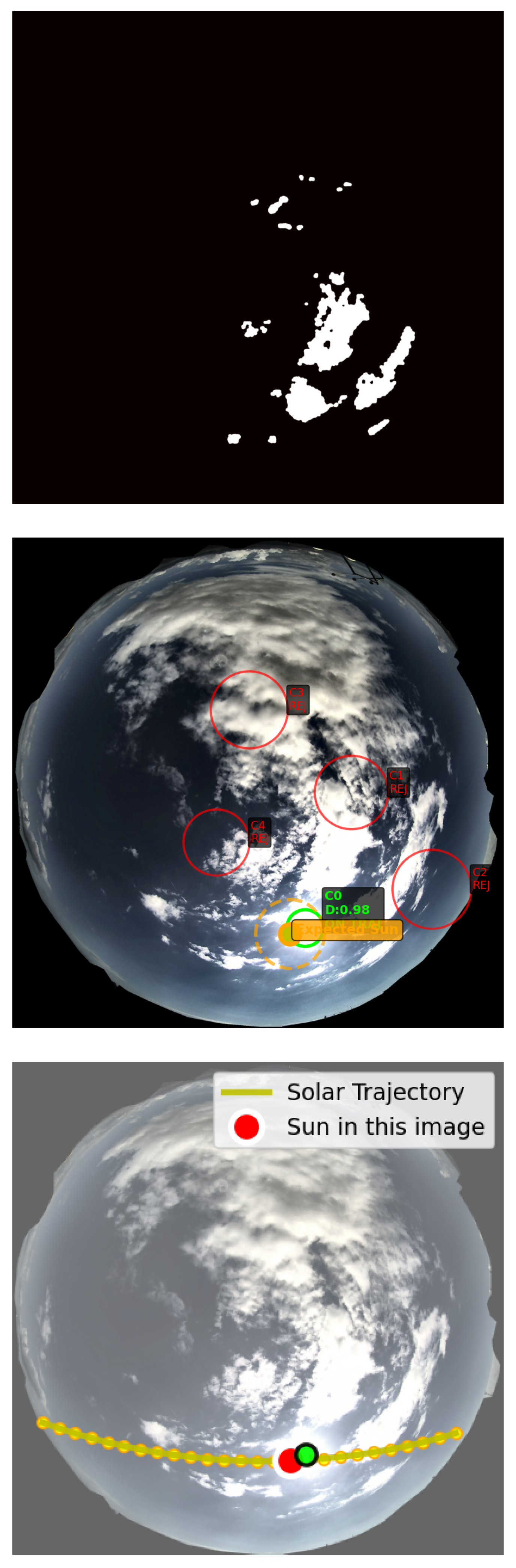
Figure 3 illustrates the complete sun detection pipeline, showing the progression from brightness masking through candidate validation to final trajectory confirmation.

Figure 3. Pipeline of the sun detection algorithm showing preprocessing, candidate detection, and trajectory validation stages.

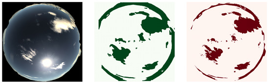
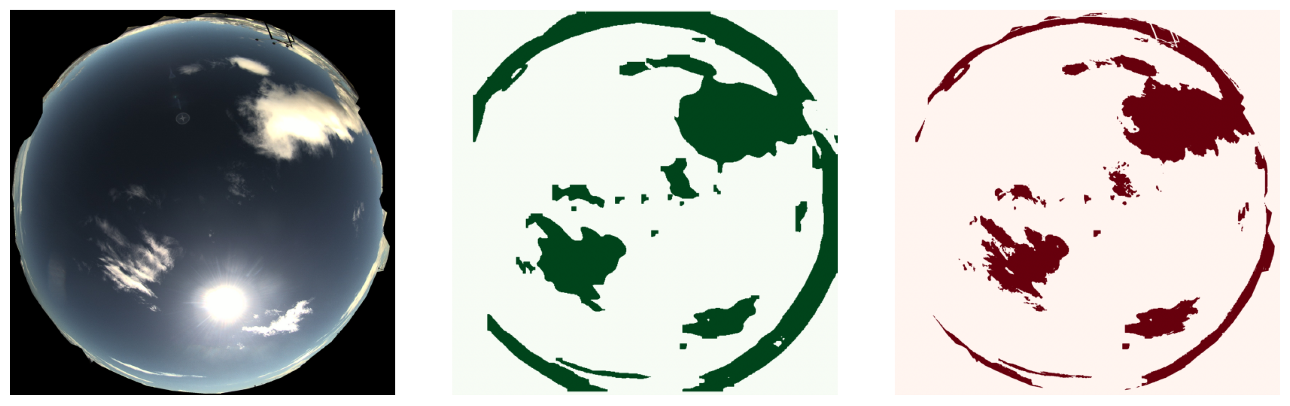
The pipeline demonstrates the image preprocessing steps applied to optimize sun position detection under varying atmospheric conditions, including CLAHE contrast enhancement and bilateral filtering to reduce noise while maintaining sharp boundaries. The Hough circle detection stage shows candidate validation through trajectory matching, with rejected candidates (red) due to distance exceeding the tolerance threshold of 150 pixels, while accepted candidates (green) match the predicted solar position (orange marker). The final validation stage confirms that the detected sun position aligns with the computed solar trajectory from pvlib calculations, ensuring accurate sun exclusion for cloud segmentation.

Each of the three images in Figure 3 summarizes multiple stages of the algorithm: the first image combines stages 1–3 (brightness masking, early rejection, and morphological filtering), showing the result of preprocessing; the second image integrates stages 4–6 (Hough circle detection, trajectory validation, and density validation), presenting the detected candidates with their respective validations; and the third image corresponds to stage 7 (sun mask creation), showing the accepted sun in green, the sun estimated by the algorithm in red, and the calculated solar trajectory.

2.2. Traditional Computer Vision Methods: Initial Attempts

Before developing the hybrid approach, traditional computer vision methods applied globally to fisheye images were investigated. These methods were tested without excluding the sun region in order to fully assess their performance and limitations. This section documents these initial attempts and the insights that motivated the development of the hybrid methodology.

2.2.1. HSV Thresholding

HSV color space provides an intuitive representation for cloud segmentation by separating chromatic information consisting of Hue and Saturation from intensity represented by Value. A single comprehensive threshold range covering all cloud types is defined:

$$\begin{array}{cc}\hfill \mathrm{Cloud}{\mathrm{Mask}}_{\mathrm{HSV}}=\left\{\right(H,S,V):& 0\le H\le 179,\hfill \\ \hfill & 0\le S\le 120,\hfill \\ \hfill & 40\le V\le 255\}\hfill \end{array}$$

(9)

Additionally, highly saturated blue sky regions are excluded:

$$\begin{array}{cc}\hfill \mathrm{Blue}\mathrm{Sky}\mathrm{Mask}=\left\{\right(H,S,V):& 80\le H\le 140,\hfill \\ \hfill & 61\le S\le 255,\hfill \\ \hfill & 40\le V\le 255\}\hfill \end{array}$$

(10)

The final cloud mask is: $M_{\mathrm{cloud}}^{\mathrm{HSV}}=\mathrm{Cloud}{\mathrm{Mask}}_{\mathrm{HSV}}\wedge \neg \mathrm{Blue}\mathrm{Sky}\mathrm{Mask}$.

This resulting binary mask identifies pixels that meet the cloud criteria (according to the defined HSV thresholds) but excludes regions of highly saturated blue sky. The logical AND operation ∧ combines both conditions, while the NOT operation ¬ inverts the blue sky mask to exclude those regions from the final result. The output is a binary image where white pixels represent detected clouds and black pixels represent clear sky or excluded regions.

Limitations of HSV Thresholding

Although HSV thresholding works reasonably well under stable atmospheric conditions, it does not perform equally when there is ambiguity in pixel representation. Whitish-blue tones can represent either thin clouds or clear sky, depending on viewing angle, atmospheric haze, and sun position. Static thresholds cannot adapt to these variations without additional information (e.g., from other sensors), resulting in over-segmentation (classifying clear sky as clouds) or under-segmentation (missing thin clouds). Therefore, this is a key consideration when addressing cloud identification in these fisheye devices.

2.2.2. K-Means Clustering with Adapted Centroids

To address the limitations of fixed thresholds, K-means clustering [26] is implemented in the HSV color space. For each image, pixels are clustered into $k=3$ classes representing sky, cloud, and sun or bright regions:

$$\underset{\mathbf{C}}{\arg \min }{\displaystyle \sum _{i=1}^k}\sum _{\mathbf{x}\in S_i}{\parallel \mathbf{x}-{\mathbf{c}}_i\parallel }^2$$

(11)

where $\mathbf{C}=\{{\mathbf{c}}_1,{\mathbf{c}}_2,{\mathbf{c}}_3\}$ are the cluster centroids, $S_i$ is the set of pixels assigned to cluster i, and $\mathbf{x}={[H,S,V]}^T$ is the HSV feature vector.

Cloud classification is based on centroid characteristics: clusters with high V and low S are classified as clouds, while high S and moderate V indicate sky.

Limitations of K-Means Clustering

K-means provides more adaptability than fixed thresholds but still produces suboptimal results. The algorithm struggles with gradual transitions between cloud and sky, where clustering assigns pixels definitively; it is sensitive to initialization, affecting consistency across images, and cannot distinguish between thin cirrus clouds and hazy sky regions with similar color distributions.

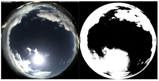
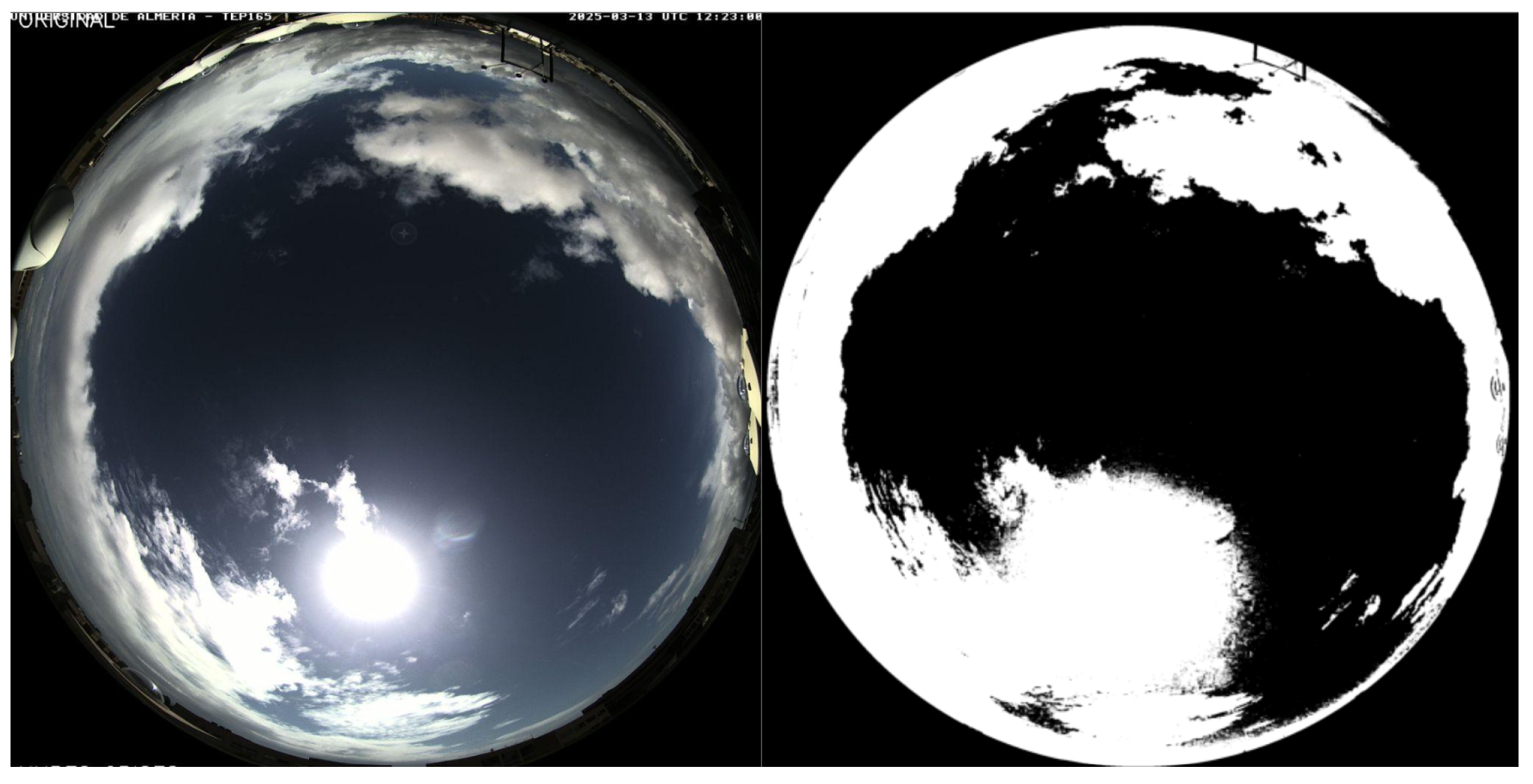
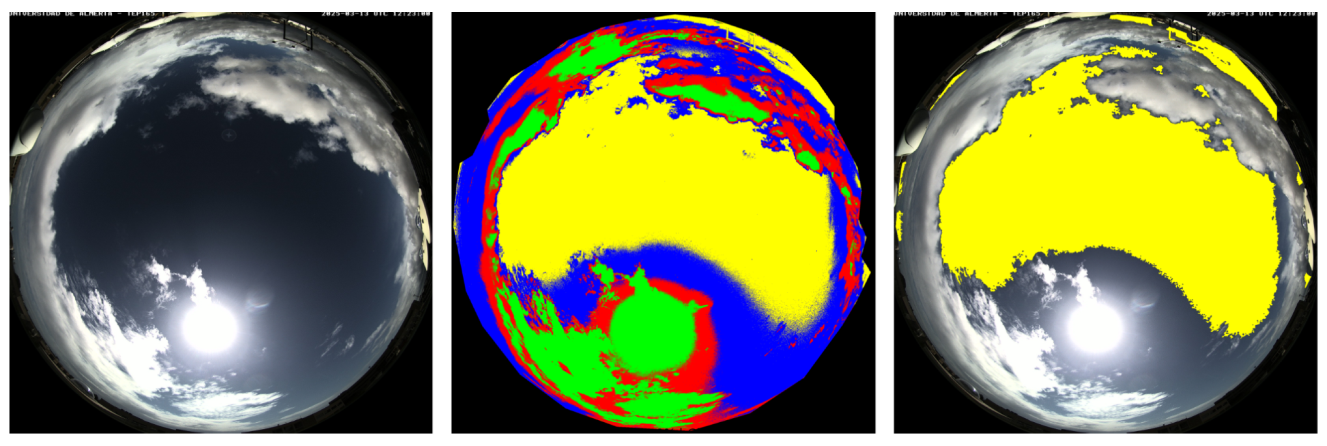
Figure 4 and Figure 5 illustrate the results and limitations of these traditional approaches when applied globally to fisheye images, without sun detection and exclusion, to clearly show how these methods work without that correction.

Figure 4. HSV thresholding results showing original fisheye image and binary cloud mask.

Figure 5. K-means clustering results with k = 4 showing original image, color-coded segmentation, and visualization.

The HSV thresholding method demonstrates over-segmentation in ambiguous sky regions and misclassifies the sun disk as cloud due to similar brightness values. The K-means approach struggles with gradual cloud–sky transitions and initialization sensitivity, leading to inconsistent segmentation. Both methods cannot distinguish between thin cirrus clouds and hazy sky regions with similar color distributions, demonstrating the limitations of global thresholding approaches.

Figure 4 and Figure 5 provide the visual motivation for the proposed hybrid design. When the HSV criterion is applied globally, every pixel satisfying the low-saturation and brightness conditions is accepted irrespective of whether it belongs to a coherent cloud structure; consequently, bright or weakly saturated clear sky regions can be included in the cloud mask. K-means changes the decision rule but still partitions the full image using color statistics without an object-level constraint. The hybrid method introduces this missing constraint: instead of accepting the global HSV mask $M_{\mathrm{HSV}}$ throughout the fisheye image, it retains HSV-positive pixels only where the YOLOv8 instance segmentation has supplied cloud support, i.e., $M_{\mathrm{YOLO}}\wedge M_{\mathrm{HSV}}$, with the solar mask subsequently excluded. Thus, the traditional method figures explain why HSV is retained for local boundary delineation but is not used as a global cloud detector.

2.3. Hybrid Approach: YOLOv8 + HSV Refinement

Building on the global failure modes illustrated in the preceding subsection, the hybrid pipeline separates cloud localization from local boundary delineation. YOLOv8 first supplies the spatial support in which cloud-like structures occur; HSV is then used only to refine the spectral boundary within that support. The following subsections define this contextual decision formally and describe its implementation.

2.3.1. Formal Definition of Contextual Information

In this work, contextual information is defined as the image-level and neighborhood information used to determine whether local spectral evidence belongs to a cloud object. In contrast to HSV thresholding, which evaluates each pixel from its color vector, the YOLOv8 segmentation model estimates cloud-support regions from learned visual cues that include spatial extent, texture, morphology, continuity, and the relationship of a pixel to its surrounding region. Let $M_{\mathrm{YOLO}}={\bigcup }_{i=1}^n{M}_i$ denote the union of the instance masks predicted by YOLOv8, $M_{\mathrm{HSV}}$ the binary mask resulting from the HSV criterion, and $M_s$ the solar-exclusion mask. Before the final morphological-cleaning step, the contextual decision rule is:

$${\widehat{M}}_{\mathrm{cloud}}=M_{\mathrm{YOLO}}\wedge M_{\mathrm{HSV}}\wedge \neg M_s.$$

(12)

Thus, the same HSV vector can be accepted as a cloud when it occurs within a cloud-support region $M_{\mathrm{YOLO}}$ and rejected when it occurs outside that region. The solar mask adds an independent geometric constraint by excluding pixels associated with the predicted solar position. In this formulation, context is not an informal attribute; it is operationally represented by the learned spatial support $M_{\mathrm{YOLO}}$ that gates the local spectral decision.

The three components also have distinct physical and methodological roles. HSV thresholding provides local spectral evidence: under clear sky conditions, molecular Rayleigh scattering generally produces a blue, relatively saturated radiance field, whereas cloud particles scatter radiation more broadly and commonly yield brighter, less saturated or more neutral pixel values [6,11]. This evidence is empirical rather than a complete physical retrieval and can be altered by aerosol loading, thin clouds, exposure control, camera color processing, and circumsolar glare. YOLOv8 does not encode an atmospheric radiative-transfer law; instead, it learns visual and spatial regularities from the annotated images and supplies the contextual support for the local HSV decision. Finally, pvlib contributes an explicit physical–geometric constraint by predicting the solar position from time and site coordinates, thereby identifying the region in which sensor saturation and bloom may otherwise resemble bright cloud pixels [23,24]. The components are therefore complementary: HSV supplies spectral evidence, YOLOv8 supplies learned spatial context, and pvlib supplies solar geometry.

2.3.2. YOLO Architecture for Contextual Segmentation

You Only Look Once (YOLO) architectures offer several advantages for cloud detection: fine-tuning with small datasets (hundreds to thousands of images) using transfer learning, single-stage detection enabling >30 fps on modern GPUs suitable for operational forecasting, and pixel-level masks in addition to bounding boxes. When trained on diverse atmospheric conditions, YOLO learns robust cloud detection features.

Zhu et al. [19] found that YOLOv5-l achieved higher recognition rates (>95%) with fewer missed detections in remote sensing images, while YOLOv8 showed slightly higher mean Average Precision. However, in ground-based fisheye images, YOLOv8 consistently outperformed YOLOv5 across all metrics. This discrepancy likely arises from differences in image characteristics, cloud types, and evaluation priorities, with the dataset emphasizing precise boundary detection favoring YOLOv8’s precision-oriented behavior.

2.3.3. YOLOv8 Training Configuration

YOLOv8l-seg, the large segmentation variant, was used with the following training configuration:

• Dataset: 150 images in total, split into 120 training images and 30 validation images (following the 80/20% convention).
• Training epochs: 700.
• nput resolution: 640 × 640 pixels, resized from the native fisheye resolution.
• Data augmentation: Random horizontal flips (fliplr = 0.5), brightness and contrast adjustment (hsv_v = 0.4, hsv_s = 0.7), mosaic augmentation (mosaic = 1.0), and image mixing (mixup = 0.1). These techniques artificially increase dataset diversity to improve model generalization.
• Optimizer: Stochastic Gradient Descent (SGD) with momentum = 0.937 and weight decay = 0.0005. The high momentum (0.937) helps maintain the optimization direction in noisy gradients, while weight decay prevents overfitting by regularizing model weights.
• Learning rate: Initial learning rate = 0.01 with cosine annealing. This configuration is conservative but stable: the moderate initial rate avoids excessive oscillations, while cosine annealing gradually reduces the learning rate following a cosine function, allowing fine parameter refinement in the final epochs.

2.3.4. YOLOv8 Performance Metrics

Table 1 summarizes the performance metrics for both bounding box detection (box) and instance segmentation (mask).

Table 1. YOLOv8l-seg performance metrics on validation set (best model).

Metric Type	Precision	Recall	mAP@0.5	mAP@0.5:0.95
Bounding Box	0.715	0.622	0.680	0.436
Instance Mask	0.821	0.537	0.656	0.337

• Mask precision of 0.821: Indicates high confidence in detected cloud regions, minimizing false positives.
• Box mAP@0.5 of 0.680: Demonstrates good detection capability at an Intersection over Union (IoU) threshold of 0.5. The IoU measures the overlap between the prediction and the ground truth annotation, calculated as $\mathrm{IoU}={\displaystyle \frac{\mathrm{Intersection}\mathrm{Area}}{\mathrm{Union}\mathrm{Area}}}$.
• Lower mAP@0.5:0.95: The drop in mean Average Precision for stricter IoU thresholds, with box at 0.436 and mask at 0.337, is typical for objects with soft boundaries like clouds. Exact delineation of cloud edges is inherently ambiguous even for human annotators.
• Moderate recall: Recall values are 0.622 for box detection and 0.537 for mask segmentation, indicating room for improvement in detecting all cloud instances, particularly small or thin clouds. This is acceptable for the hybrid approach since HSV refinement operates within detected regions.

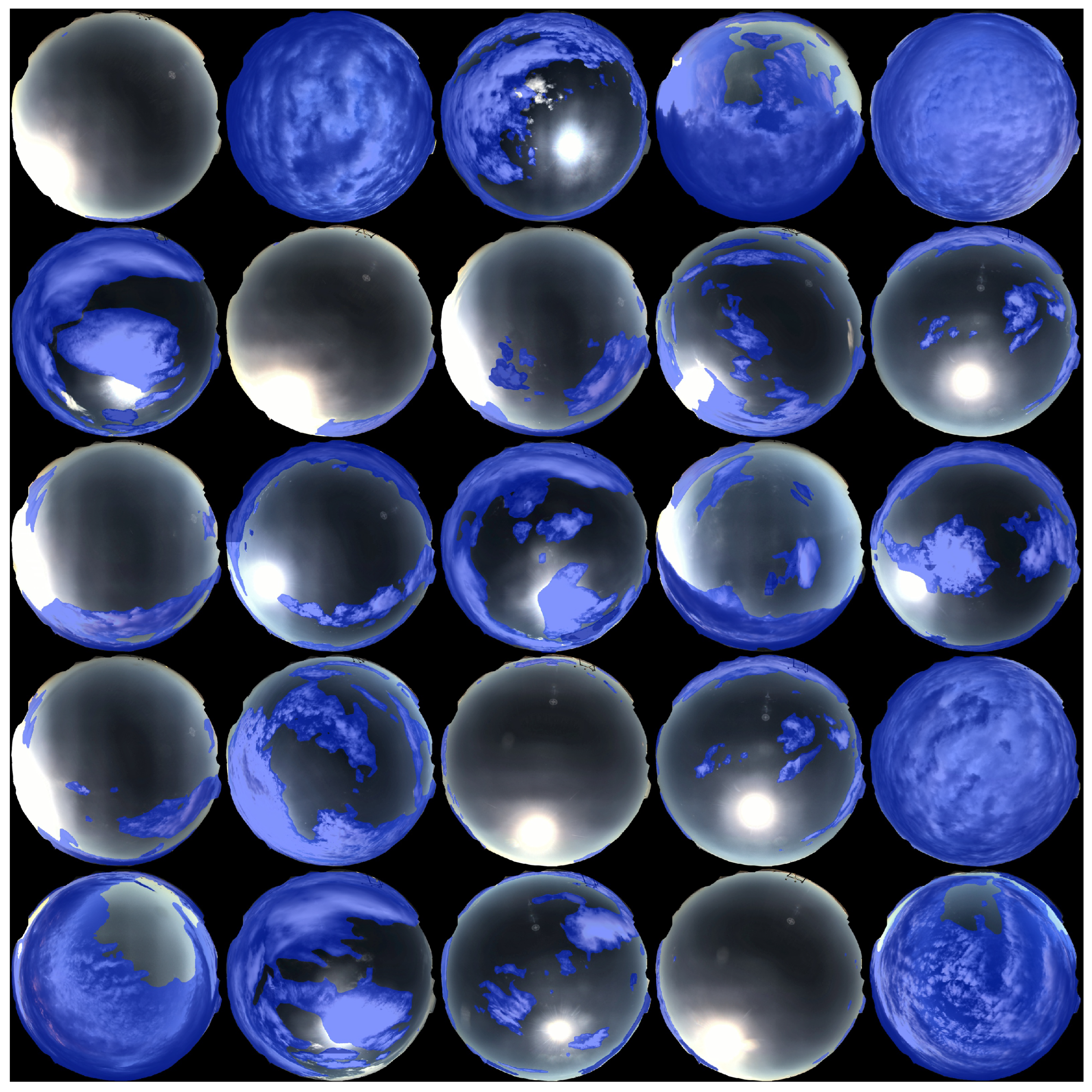
The training metrics demonstrate stable convergence across 700 epochs with consistent improvement in both box and mask precision. Figure 6 presents representative validation predictions as mask overlays only, allowing the spatial extent of the predicted cloud instances to be inspected without the visual clutter of confidence labels and bounding boxes.

Figure 6. Representative validation images showing predicted cloud instance masks across diverse atmospheric conditions.

2.3.5. HSV Refinement Within YOLO Regions

After the cloud-support masks have been predicted, the implementation applies the HSV thresholds of Equation (9) to each instance mask $M_i$, as specified in Algorithm 1. This stage operationalizes the contextual decision rule in Equation (12): it does not perform another global cloud search, but retains only the HSV-positive pixels within the YOLOv8 support before the solar-exclusion and morphological-cleaning steps.

Algorithm 1 formalizes the hybrid segmentation procedure.

Algorithm 1 Hybrid cloud segmentation

Require: Fisheye image I, YOLOv8 model $\mathcal{M}$, HSV thresholds ${\Theta }_{\mathrm{HSV}}$ Ensure: Refined cloud mask $M_{\mathrm{final}}$

1: Convert Red, Green, Blue (RGB) image I to HSV color space: $I_{\mathrm{HSV}}\leftarrow \mathrm{RGB}2\mathrm{HSV}\left(I\right)$   2: Detect sun position and radius using solar trajectory model: $(x_s,y_s,r_s)\leftarrow \mathrm{DetectSun}(I_{\mathrm{HSV}},t,\varphi ,\lambda )$ where t is timestamp, $\varphi$ is latitude, $\lambda$ is longitude, $x_s,y_s$ are sun center coordinates, and $r_s$ is sun radius in pixels   3: Create sun exclusion mask with expanded radius: $M_s\leftarrow \mathrm{CreateCircleMask}(x_s,y_s,1.15\times r_s)$   4: Detect cloud regions using YOLOv8: $\{R_1,R_2,\dots ,R_n\}\leftarrow \mathcal{M}\left(I\right)$ where each $R_i$ is a detected cloud instance with associated mask   5: Initialize final cloud mask as zero matrix: $M_{\mathrm{final}}\leftarrow \mathbf{0}$   6: for each detected region $R_i$ where $i\in \{1,2,\dots ,n\}$ do   7:      Extract binary mask from region instance: $M_i\leftarrow R_i.\mathrm{mask}$   8:      Apply HSV thresholding within detected region using logical AND: $M_{\mathrm{cloud}}^i\leftarrow \mathrm{HSVThreshold}(I_{\mathrm{HSV}},{\Theta }_{\mathrm{HSV}})\wedge M_i$   9:      Exclude sun pixels using logical AND with negated sun mask: $M_{\mathrm{cloud}}^i\leftarrow M_{\mathrm{cloud}}^i\wedge \neg M_s$ 10:      Accumulate refined cloud mask using logical OR: $M_{\mathrm{final}}\leftarrow M_{\mathrm{final}}\vee M_{\mathrm{cloud}}^i$ 11: end for 12: Apply morphological operations for noise removal: $M_{\mathrm{final}}\leftarrow \mathrm{MorphClean}\left(M_{\mathrm{final}}\right)$ 13: return Final binary cloud segmentation mask $M_{\mathrm{final}}$

The hybrid approach provides several key advantages. HSV thresholding operates within semantically meaningful cloud regions identified by YOLOv8, enabling context-aware refinement. Traditional methods excel at local boundary refinement but fail at global classification, and the hybrid system leverages this strength. Processing HSV thresholds only within YOLO regions, typically 20–40% of the image area, restricts the spectral decision to cloud-like support regions and reduces the amount of image area considered by the refinement stage.

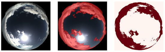
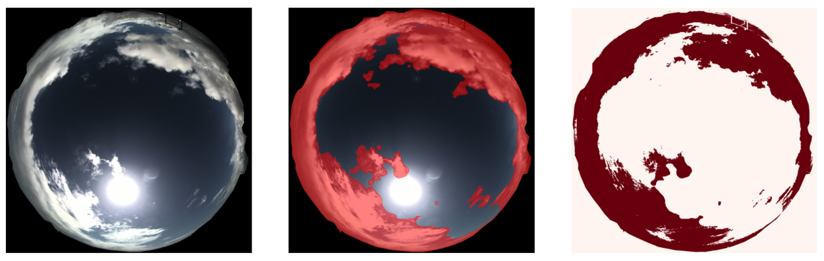
Figure 7 visualizes the successive stages of the proposed pipeline: the original image, the YOLOv8 contextual support, and the final HSV-refined mask.

Figure 7. Progressive segmentation pipeline showing original image, YOLOv8 detection, and hybrid refinement.

The progressive segmentation pipeline provides a qualitative illustration of the distinct roles of the two stages. In the middle panel, YOLOv8 identifies the cloud at the coarse instance level and supplies a spatial support that includes the relevant cloud structure, rather than attempting to resolve every ambiguous boundary pixel. In the final panel, the same HSV criterion is evaluated only within that support, allowing the local spectral transition to determine the detailed cloud boundary while rejecting spectrally similar pixels outside the YOLO region. The figure therefore makes the intended division of labor visible: YOLOv8 answers the question of where cloud-like structures occur, whereas HSV refines which pixels within these structures satisfy the cloud criterion. This visual comparison illustrates the mechanism of the hybrid method but does not, by itself, quantify its pixel-level effect relative to YOLOv8 alone.

3. Results

3.1. Dataset and Ground Truth

For the first model developed in this work, the training dataset consists exclusively of fisheye images captured by a Mobotix Q71camera at CIESOL under diverse atmospheric conditions, including clear sky, scattered clouds, and overcast and hazy conditions. All training images were captured during daytime hours with solar elevation above 5° to ensure adequate lighting for cloud detection.

For validation, the methodology was evaluated on images from two additional locations:

• University of Antofagasta, Chile: Images captured with Mobotix Q25 hemispheric camera featuring a 6-megapixel sensor and HD fisheye lens with low power consumption and resistance to adverse conditions.
• University of Huelva, Spain: Images obtained with EKO ASI-16 system, an automatic hemispheric camera with a 5-megapixel fisheye lens, quartz dome with anti-reflective coating, thermal control, and high-resolution High Dynamic Range (HDR) capability.

These sites were used exclusively to test generalization capabilities without retraining, evaluating robustness across different locations and camera systems.

3.2. Comparison of Instance-Segmentation Backbones

The initial choice of YOLOv8l-seg was motivated by its single-stage instance-segmentation capability, which supplies the cloud-support masks required by the context-gated HSV refinement while retaining an operationally suitable inference workflow. To verify that this selection remains appropriate relative to newer alternatives, YOLOv8l-seg is compared with YOLO11l-seg, YOLO26l-seg, and RF-DETR Seg Large. All models were trained on the same cloud image dataset and data split for 700 epochs. RF-DETR Seg Large used a batch size of four because of its substantially higher memory demand; its learning rate and weight decay were ${10}^{-3}$ and $5\times {10}^{-4}$, respectively. The comparison should therefore be interpreted as a controlled dataset-level model selection study, while recognizing that each framework retains its native optimization implementation. Table 2 shows the main parameters for the different models analyzed.

Table 2. Comparison of instance-segmentation backbones on the validation split. The best value in each metric group is highlighted in bold.

Model	Output	Precision	Recall	mAP@0.5	mAP@0.5:0.95
YOLOv8l-seg	Box	0.715	0.622	0.680	0.436
YOLOv8l-seg	Mask	0.821	0.537	0.656	0.337
YOLO11l-seg	Box	0.764	0.593	0.677	0.421
YOLO11l-seg	Mask	0.743	0.575	0.636	0.337
YOLO26l-seg	Box	0.788	0.622	0.714	0.435
YOLO26l-seg	Mask	0.784	0.553	0.634	0.335
RF-DETR Seg Large	Box	0.820	0.427	0.546	0.336
RF-DETR Seg Large	Mask	0.785	0.415	0.484	0.252

YOLO26l-seg achieved the strongest bounding box detection performance, with the highest box mAP@0.5 (0.714) and an mAP@0.5:0.95 (0.435) practically identical to that of YOLOv8l-seg (0.436). However, the proposed pipeline depends primarily on reliable instance masks rather than boxes. In mask segmentation, YOLOv8l-seg achieved the highest mAP@0.5 (0.656), tied for the highest mAP@0.5:0.95 (0.337), and maintained the highest mask precision (0.821). Notably, RF-DETR Seg Large exhibited highly selective prediction behavior, retaining a competitive mask precision of 0.785 but yielding a substantially lower mask recall of 0.415. This asymmetrical performance profile, inherent to query-based attention mechanisms that prioritize high-confidence predictions, explains its lower mask mAP values. While YOLO11l-seg offered a balanced alternative and attained the highest mask recall (0.575), these results fully justify retaining YOLOv8l-seg as the backbone for the hybrid framework: its mask predictions provide the most effective trade-off between high spatial precision and robust recall, supplying optimal spatial support for the subsequent local HSV refinement.

3.3. Radiometric Validation with k_t and k_d Indices

To validate the cloud segmentation results against ground truth, radiometric indices derived from measurements taken at CIESOL were used. These indices provide objective and quantitative measures of atmospheric conditions that can be correlated with the cloud cover estimates obtained from our segmentation methods [27]. Global and diffuse irradiance measurements were performed using two CMP 11 Kipp & Zonen pyranometers installed on a dual-axis solar tracker at one-minute intervals, where the diffuse component was obtained thanks to partial shading of the radiometer using shading balls.

3.3.1. Clearness Index (k_t)

The clearness index quantifies the fraction of extraterrestrial solar irradiance reaching the ground surface:

$${\mathit{k}}_{\mathit{t}}={\displaystyle \frac{\mathrm{GHI}}{I_0·E_0·\sin \left({\alpha }_s\right)}}$$

(13)

where

• Global Horizontal Irradiance (GHI) is measured by pyranometer (W/m²);
• $I_0=1367$ W/m² = solar constant;
• ${\alpha }_s$ = solar elevation angle (degrees) from PVlib algorithm;
• $E_0$ = Earth–Sun distance correction factor.

The correction factor $E_0$ accounts for Earth’s elliptical orbit:

$$\begin{array}{cc}\hfill E_0& =1.00011+0.034221\cos \left(\psi \right)+0.00128\sin \left(\psi \right)\hfill \\ \hfill & +0.000719\cos \left(2\psi \right)+0.000077\sin \left(2\psi \right)\hfill \end{array}$$

(14)

where $\psi =2\pi (DOY-1)/365$ is the day angle and $DOY$ is the Day Of the Year.

3.3.2. Diffuse Fraction (k_d)

The diffuse fraction represents the proportion of GHI contributed by diffuse (scattered) radiation:

$${\mathit{k}}_{\mathit{d}}={\displaystyle \frac{\mathrm{DHI}}{\mathrm{GHI}}}$$

(15)

where DHI = Diffuse Horizontal Irradiance measured by pyranometer with a shadow band (W/m²).

3.3.3. Atmospheric Condition Interpretation

The relationship between k_t and k_d provides insight into atmospheric conditions [28]:

• k_t > k_d: Clear sky conditions where direct solar radiation dominates.
• k_t < k_d: Cloudy conditions where diffuse radiation dominates due to cloud scattering.
• k_t ≈ k_d: Mixed or transitional atmospheric conditions.

In this study, this relationship is considered in a binary manner, distinguishing only between clear and cloudy conditions for simplicity in subsequent analyses.

The hypothesis is that estimated cloud coverage from the segmentation algorithm should correlate with these radiometric indices: high cloud coverage should correspond to low k_t and high k_d, and vice versa.

Figure 8 and Figure 9 demonstrate the radiometric validation of the hybrid approach under contrasting atmospheric conditions, showing the complete segmentation pipeline alongside measured radiometric indices.

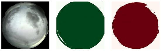
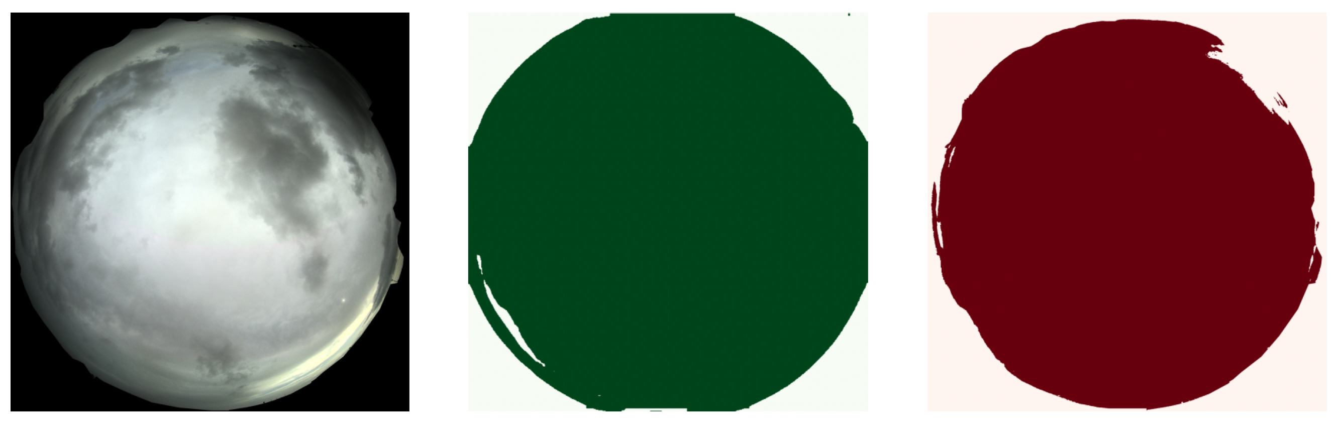
Figure 8. Cloudy sky validation showing progressive segmentation pipeline and radiometric indices.

Figure 9. Clear sky validation showing progressive segmentation pipeline and radiometric indices.

The cloudy sky validation case, captured on 7 March 2025 at 16:08:00, shows a progressive segmentation pipeline with dense cloud cover achieving 96.5% cloud coverage (3,354,504 pixels out of 3,475,827 total pixels). The radiometric indices confirm cloudy conditions with clearness index k_t = 0.119 indicating low clearness, diffuse fraction k_d = 0.999 indicating high diffuse fraction, and difference k_t − k_d = −0.880 indicating diffuse radiation dominance. The clear sky validation case, captured on 10 March 2025 at 13:16:00, demonstrates the methodology under clear conditions with scattered clouds, achieving 18.8% cloud coverage (647,395 pixels out of 3,446,302 effective sky area pixels). The radiometric indices confirm clear sky conditions, with the clearness index k_t = 0.855 indicating high clearness, diffuse fraction k_d = 0.112 indicating low diffuse fraction, and difference k_t − k_d = 0.742 indicating direct radiation dominance, with sun detection in the clear sky region.

These validation cases demonstrate strong agreement between segmentation-derived cloud coverage and radiometric measurements. The cloudy case with k_t < k_d and 96.5% coverage and the clear sky case with k_t > k_d and 18.8% coverage confirm that the hybrid approach accurately captures atmospheric conditions across the full spectrum from overcast to clear skies.

3.4. Multi-Site Generalization: Almería, Antofagasta and Huelva

A key objective of this work was to develop a methodology generalizable across geographical locations without site-specific retraining. Multi-site testing revealed important insights about the robustness of different components of the hybrid approach across different camera systems and atmospheric conditions.

Performance Across Mobotix Camera Systems

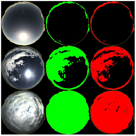
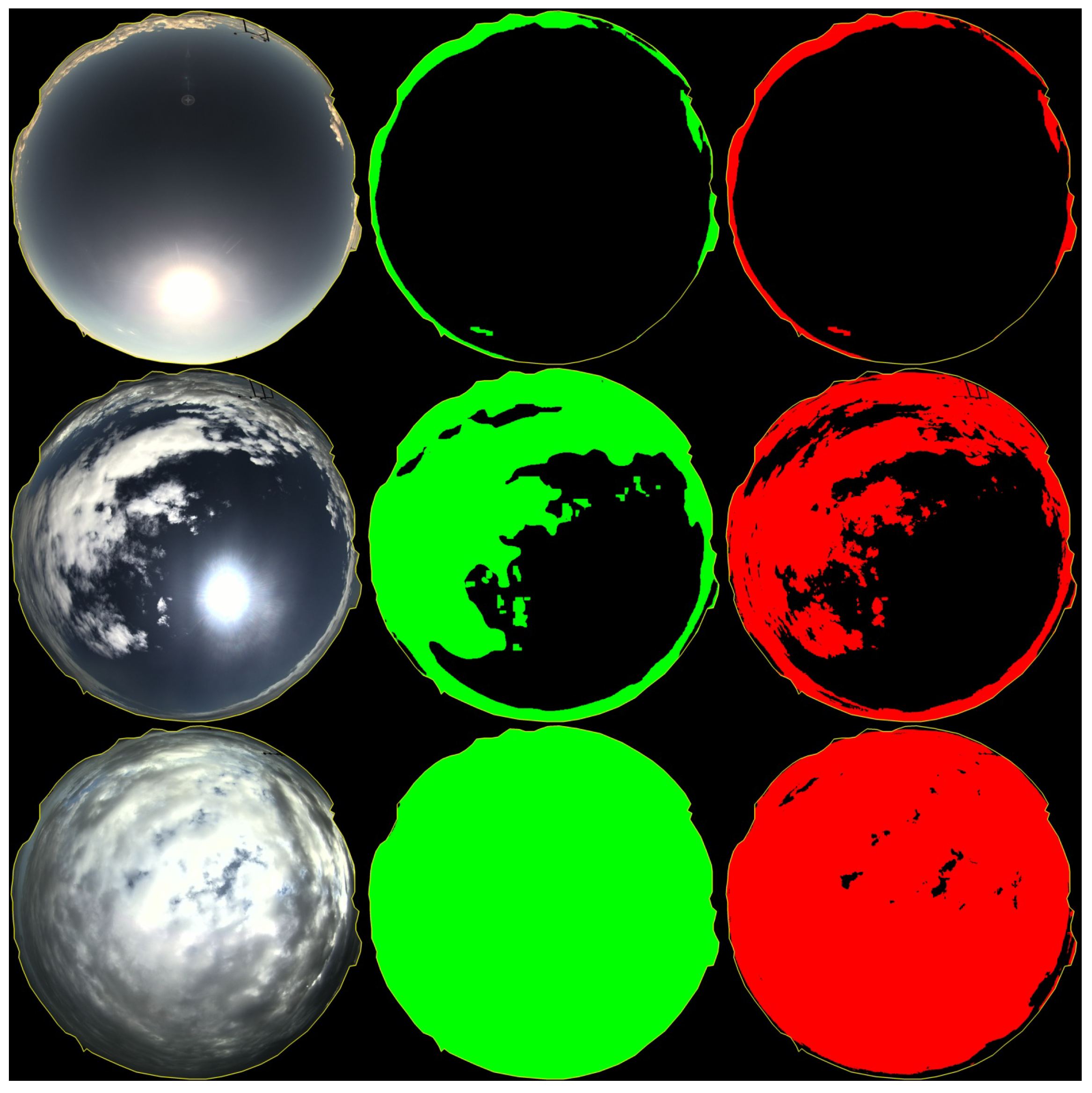
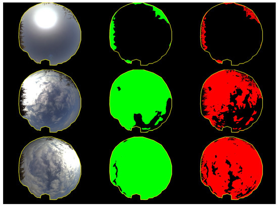
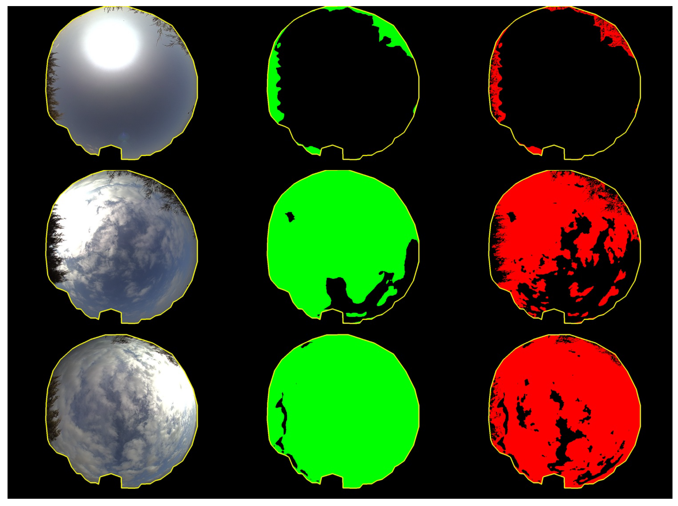
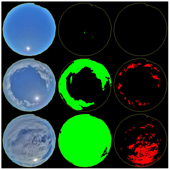
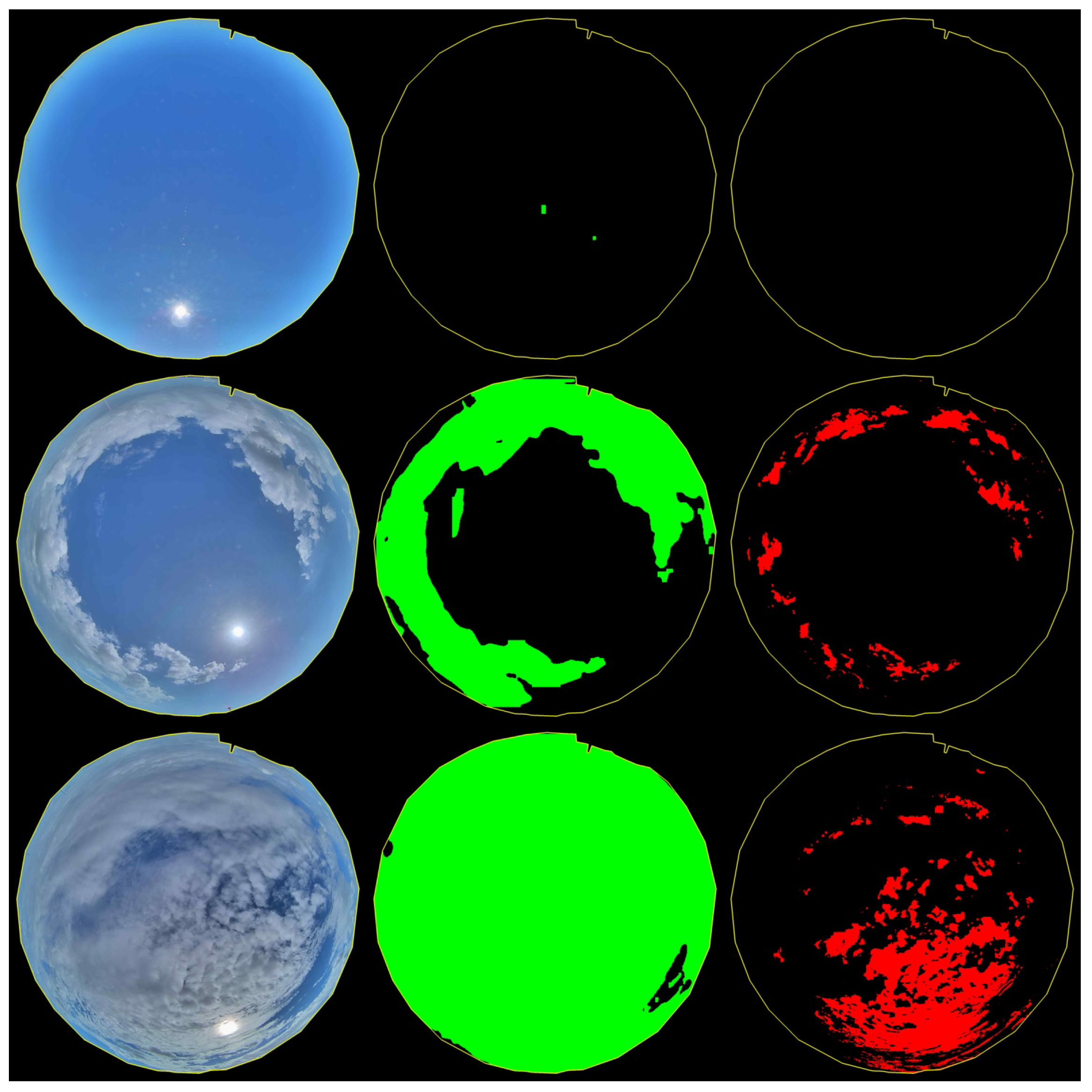
Figure 10, Figure 11 and Figure 12 demonstrate the hybrid approach’s performance at three locations, each showing a 3 × 3 grid representing different sky conditions (rows: clear, partially cloudy, overcast) and processing stages (columns: original fisheye image, YOLOv8 instance segmentation with detected cloud regions shown in green, and final hybrid segmentation combining YOLO context with HSV refinement shown in red). A yellow contour delineates the sky region boundary, defining the working area for cloud detection analysis.

Figure 10. Multi-condition performance at CIESOL (Almería, Spain) with Mobotix Q71.

Figure 11. Multi-condition performance at University of Antofagasta (Chile) with Mobotix Q25.

Figure 12. Multi-condition performance at University of Huelva (Spain) with EKO ASI-16.

Robust performance with consistent cloud detection is demonstrated across varying sky conditions: minimal false positives in clear sky conditions, precise cloud boundary delineation in partially cloudy scenarios, and comprehensive coverage detection in overcast conditions. Sun disk exclusion successfully prevents misclassification of high-brightness regions.

Remarkable generalization across geographical locations and atmospheric conditions is achieved despite training on a modest dataset. While occasional small areas may be missed due to limited training data, successful adaptation to the Southern Hemisphere context without retraining validates the convolutional neural network’s robustness across latitudes. A notable limitation is occasional tree foliage misclassification, addressable through fine-tuning.

Distinct color gamut and saturation characteristics reveal hybrid approach limitations with different camera systems. While YOLOv8 maintains robust cloud detection without retraining, HSV refinement shows significant degradation with over-segmentation in ambiguous regions and under-segmentation at boundaries. This highlights the critical sensitivity of static HSV thresholds to camera-specific calibration, while demonstrating superior CNN generalization. For cross-camera deployment, YOLO provides reliable detection, whereas HSV requires camera-specific calibration for optimal accuracy.

The multi-site validation revealed a critical distinction between the performance of different methodology components:

• YOLOv8 robustness: The convolutional neural network component demonstrated excellent generalization across all three sites, maintaining consistent cloud detection performance regardless of camera system or geographical location. Although there were occasional small areas that were not correctly detected, this could likely be addressed by retraining the model. The model was trained using a single dataset and consumer-grade equipment, which made its overall performance particularly noteworthy.
• HSV thresholding limitations: While HSV refinement performed excellently on Mobotix systems (Almería and Antofagasta), it showed reduced effectiveness on the Huelva camera system due to different color gamut and saturation characteristics. This limitation is understandable given that static thresholds are inherently sensitive to camera-specific color calibration.
• Practical implications: For local applications with consistent camera hardware (e.g., Mobotix Q71), the full hybrid approach provides optimal performance. However, for broader deployment across diverse camera systems, the YOLOv8 component alone offers significant advantages for generalization, while local HSV refinement should be calibrated per camera system for optimal results.

These findings support the conclusion that convolutional neural networks provide substantial advantages for extrapolation and cross-camera generalization, while traditional computer vision methods like HSV thresholding are most effective when calibrated for specific camera characteristics. This observation is important for large-scale solar forecasting projects, as camera hardware can vary between installations.

It is important to note that the complete processing of an image (sun detection via astronomical calculations, segmentation with YOLO, and application of HSV thresholds) is executed in a maximum of 3 s, providing near-real-time results suitable for operational solar forecasting applications. This processing time is appropriate considering that the capture interval between images is 1 min, allowing full processing of each image before the next capture.

4. Discussion and Conclusions

This paper presents a hybrid approach for cloud segmentation from ground-based fisheye imagery, combining YOLOv8 instance segmentation with HSV thresholding refinement. The methodology addresses a fundamental limitation of traditional computer vision methods: spectral ambiguity in global thresholding.

The YOLOv8l-seg model achieved a mask precision of 0.821 and box mAP@0.5 of 0.680, demonstrating multi-site generalization (Almería, Antofagasta, Huelva) and promising correlation with radiometric measurements (clearness index $k_t$ and diffuse fraction $k_d$). Restricting HSV thresholding to YOLOv8-detected cloud regions largely eliminated false positives while maintaining computational efficiency.

Multi-site validation revealed that the CNN component demonstrated excellent generalization across all sites regardless of camera system, while HSV refinement required camera-specific calibration for optimal results. This validates the CNN’s ability to learn robust, camera-agnostic features for cloud detection.

From an operational perspective, the hybrid design provides a practical computational advantage because it does not require a separate dense semantic segmentation network for final boundary refinement. A single YOLOv8 inference supplies instance-level spatial context, whereas the subsequent HSV refinement consists of inexpensive pixel-wise operations restricted to the detected cloud regions. This division of roles avoids applying a high-capacity dense segmentation procedure to the full fisheye image solely to obtain fine cloud boundaries. On the RTX 4070 Ti platform used in this study, the complete pipeline, including solar-position-based sun exclusion, YOLO inference, and HSV refinement, requires at most 3 s per image, which is well below the 1 min image acquisition interval. The method is therefore suitable for near-real-time operational sky monitoring and solar forecasting applications.

Several limitations define the current scope of the study. First, the training dataset is modest in size and is principally drawn from one site; it cannot fully represent the variability in cloud microphysics, aerosol conditions, solar elevations, and seasonal illumination encountered in broader deployment. Second, although the multi-site examples demonstrate qualitative transferability, they are not accompanied by manually delineated reference masks at the external sites and therefore do not provide a quantitative cross-camera accuracy assessment. Third, the radiometric analysis is a preliminary consistency check based on representative clear and cloudy cases, rather than a time-series statistical validation of cloud fraction against irradiance indices.

The HSV component remains sensitive to the camera spectral response, exposure and color processing pipeline, as illustrated by its degradation for the EKO ASI-16 images. The method may also be affected by the intrinsic ambiguity of thin cloud, haze, and circumsolar regions; imperfect fisheye projection or camera alignment; and non-sky occlusions such as vegetation or horizon objects. In addition, the present frame-by-frame implementation does not exploit temporal cloud motion or continuity, and no direct latency benchmark against dense semantic segmentation architectures has been performed.

Future work should therefore establish a larger, seasonally diverse, multi-site dataset with independent test partitions and manually annotated cloud masks; quantify the YOLO-only, global-HSV, and hybrid variants using pixel-level metrics; calibrate or adapt the HSV criterion to each camera; and evaluate temporal models for cloud motion and solar nowcasting. Further priorities are deployment measurements on edge hardware, direct computational comparison with dense segmentation networks under a common protocol, and assessment of whether improved segmentation produces measurable gains in irradiance and photovoltaic-power forecasts.

Key contributions include a mathematical framework for sun detection using pvlib solar trajectory modeling; demonstration that context-aware HSV thresholding within YOLO-detected regions substantially reduces spectral ambiguity; validation against ground truth radiometric measurements; and multi-site generalization without retraining. These findings support the view that CNNs provide substantial advantages for cross-camera generalization, while traditional methods require camera-specific calibration.

References

- International Energy Agency. Renewables 2021; IEA: Paris, France, 2021; Licence: CC BY 4.0. [Google Scholar]
- Inman, R.H.; Pedro, H.T.; Coimbra, C.F. Solar forecasting methods for renewable energy integration. Prog. Energy Combust. Sci. 2013, 39, 535–576. [Google Scholar] [CrossRef] [Scilit]
- Sanchez, G.; Serrano, A.; Cancillo, M. Effect of cloudiness on solar global, solar diffuse and terrestrial downward radiation at Badajoz (Southwestern Spain). Opt. Pura Apl. 2012, 45, 33–38. [Google Scholar] [CrossRef] [Scilit]
- Tzoumanikas, P.; Nikitidou, E.; Bais, A.; Kazantzidis, A. The effect of clouds on surface solar irradiance, based on data from an all-sky imaging system. Renew. Energy 2016, 95, 314–322. [Google Scholar] [CrossRef] [Scilit]
- Chow, C.; Urquhart, B.; Lave, M.; Dominguez, A.; Kleissl, J.; Shields, J.; Washom, B. Intra-hour forecasting with a total sky imager at the UC San Diego solar energy testbed. Sol. Energy 2011, 85, 2881–2893. [Google Scholar] [CrossRef] [Scilit]
- Long, C.N.; Sabburg, J.M.; Calbó, J.; Pagès, D. Retrieving Cloud Characteristics from Ground-Based Daytime Color All-Sky Images. J. Atmos. Ocean. Technol. 2006, 23, 633–652. [Google Scholar] [CrossRef] [Scilit]
- Alonso, J.; Batlles, F.; López, G.; Ternero, A. Sky camera imagery processing based on a sky classification using radiometric data. Energy 2014, 68, 599–608. [Google Scholar] [CrossRef] [Scilit]
- Alonso-Montesinos, J.; Batlles, F.; Portillo, C. Solar irradiance forecasting at one-minute intervals for different sky conditions using sky camera images. Energy Convers. Manag. 2015, 105, 1166–1177. [Google Scholar] [CrossRef] [Scilit]
- Alonso-Montesinos, J.; Batlles, F. The use of a sky camera for solar radiation estimation based on digital image processing. Energy 2015, 90, 377–386. [Google Scholar] [CrossRef] [Scilit]
- Alonso-Montesinos, J. Real-Time Automatic Cloud Detection Using a Low-Cost Sky Camera. Remote Sens. 2020, 12, 1382. [Google Scholar] [CrossRef] [Scilit]
- Dev, S.; Lee, Y.H.; Winkler, S. Color-based Segmentation of Sky/Cloud Images From Ground-based Cameras. arXiv 2016, arXiv:1606.03669. [Google Scholar] [CrossRef] [Scilit]
- Escalona-Llaguno, M.; López, G.; Ortega, G.; Alonso-Montesinos, J.; Polo, J.; Ballestrín, J. Automatic discrimination between haze and cloudiness in all sky camera images. In Proceedings of the 10th Spanish-Portuguese Assembly of Geodesy and Geophysics—Toledo, Madrid, Spain, 23 November 2022; pp. 781–790. [Google Scholar] [CrossRef] [Scilit]
- Chauvin, R.; Nou, J.; Thil, S.; Traoré, A.; Grieu, S. Cloud Detection Methodology Based on a Sky-imaging System. Energy Procedia 2015, 69, 1970–1980. [Google Scholar] [CrossRef] [Scilit]
- Yin, D.; Wang, J.; Zhai, K.; Zheng, J.; Qiang, H. Ground-Based Cloud Image Segmentation Method Based on Improved U-Net. Appl. Sci. 2024, 14, 11280. [Google Scholar] [CrossRef] [Scilit]
- Li, Y.; Wang, H.; Wang, S.; Xu, J.; Lee, Y.H.; Dev, S. BSANet: A Bilateral Segregation and Aggregation Network for Real-time Cloud Segmentation. Remote Sens. Appl. Soc. Environ. 2025, 38, 101536. [Google Scholar] [CrossRef] [Scilit]
- Fabio, L.; Piga, D.; Umberto, M.; Safouane, E.G. BenchCloudVision: A Benchmark Analysis of Deep Learning Approaches for Cloud Detection and Segmentation in Remote Sensing Imagery. arXiv 2024, arXiv:2402.13918. [Google Scholar] [CrossRef] [Scilit]
- Huo, Y.; Dong, Y.; Wang, C.; Zhang, M.; Wang, H. Multi-scale memory network with separation training for hyperspectral anomaly detection. Inf. Process. Manag. 2026, 63, 104494. [Google Scholar] [CrossRef] [Scilit]
- Qu, K.; Luo, X.; Bao, W. DNMF-AG: A Sparse Deep NMF Model with Adversarial Graph Regularization for Hyperspectral Unmixing. Remote Sens. 2026, 18, 155. [Google Scholar] [CrossRef] [Scilit]
- Zhu, X.; Ji, W.; Wu, F.; Xiang, R.; Chen, W. YOLO Based Cloud Region Recognition Algorithm for Remote Sensing Images*. In Proceedings of the 2024 IEEE International Conference on Real-Time Computing and Robotics (RCAR), Alesund, Norway, 24–28 June 2024; pp. 155–159. [Google Scholar] [CrossRef] [Scilit]
- Li, Q.; Lu, W.; Yang, J. A Hybrid Thresholding Algorithm for Cloud Detection on Ground-Based Color Images. J. Atmos. Ocean. Technol. 2011, 28, 1286–1296. [Google Scholar] [CrossRef] [Scilit]
- Hasenbalg, M.; Kuhn, P.; Wilbert, S.; Nouri, B.; Kazantzidis, A. Benchmarking of six cloud segmentation algorithms for ground-based all-sky imagers. Sol. Energy 2020, 201, 596–614. [Google Scholar] [CrossRef] [Scilit]
- Alonso, J.; Batlles, F.; Villarroel, C.; Ayala, R.; Burgaleta, J. Determination of the sun area in sky camera images using radiometric data. Energy Convers. Manag. 2014, 78, 24–31. [Google Scholar] [CrossRef] [Scilit]
- Holmgren, W.; Hansen, C.; Mikofski, M. pvlib python: A python package for modeling solar energy systems. J. Open Source Softw. 2018, 3, 884. [Google Scholar] [CrossRef] [Scilit]
- Reda, I.; Andreas, A. Solar position algorithm for solar radiation applications. Sol. Energy 2004, 76, 577–589. [Google Scholar] [CrossRef] [Scilit]
- Duda, R.O.; Hart, P.E. Use of the Hough transformation to detect lines and curves in pictures. Commun. ACM 1972, 15, 11–15. [Google Scholar] [CrossRef] [Scilit]
- Lloyd, S. Least squares quantization in PCM. IEEE Trans. Inf. Theory 1982, 28, 129–137. [Google Scholar] [CrossRef] [Scilit]
- Alados-Arboledas, L.; Batlles, F.; Olmo, F. Solar radiation resource assessment by means of silicon cells. Sol. Energy 1995, 54, 183–191. [Google Scholar] [CrossRef] [Scilit]
- Perez, R.; Ineichen, P.; Seals, R.; Michalsky, J.; Stewart, R. Modeling daylight availability and irradiance components from direct and global irradiance. Sol. Energy 1990, 44, 271–289. [Google Scholar] [CrossRef] [Scilit]
Disclaimer/Publisher’s Note: The statements, opinions and data contained in all publications are solely those of the individual author(s) and contributor(s) and not of MDPI and/or the editor(s). MDPI and/or the editor(s) disclaim responsibility for any injury to people or property resulting from any ideas, methods, instructions or products referred to in the content. |
© 2026 by the authors. Licensee MDPI, Basel, Switzerland. This article is an open access article distributed under the terms and conditions of the Creative Commons Attribution (CC BY) license.