


Highlights
What are the main findings?
- SDRCNet integrates structure-guided feature learning, label-aware multi-granularity evidence aggregation, and dual-relation consensus reasoning for multi-label remote sensing scene classification.
- SDRCNet achieves 79.3% mAP and 83.7% OF1 on China-MAS-50k, and 70.5% mAP and 75.9% OF1 on MultiScene-Clean while using only 1.13 GFLOPs and 3.82M parameters on China-MAS-50k.
What are the implications of the main findings?
- Explicitly modeling spatial structures and both cooperative and competitive label relations improves recognition reliability in complex remote sensing scenes with mixed scales, ambiguous structures, and coexisting categories.
- The proposed lightweight design provides a practical accuracy–efficiency trade-off for large-scale multi-label interpretation of very-high-resolution satellite and aerial images.
Abstract
Multi-label classification of very-high-resolution remote sensing scenes is difficult not only because multiple land-cover categories coexist in one image, but also because their discriminative evidence is spatially uneven: boundaries, elongated structures, and fragmented regions are often weakened by appearance-dominated features; small categories can be suppressed by global scene responses; and large-area categories require broader spatial context. These spatial ambiguities are further complicated by label dependencies, where co-occurring categories may support each other while visually similar categories may compete under weak or incomplete local evidence. To address these coupled challenges, we propose SDRCNet, a lightweight structure-guided dual-relation consensus network for multi-label remote sensing scene classification. First, SDRCNet introduces structure-guided feature learning to strengthen boundary, directional, and regional structural cues while maintaining an efficient network design. Second, it learns label-aware query representations and aggregates multi-granularity evidence from global scene context, local detail responses, and regional patterns, enabling different categories to obtain evidence from suitable spatial scales. Third, an evidence-aware relation reasoning mechanism models both category correlations and category competitions, allowing the network to exploit supportive label context while suppressing conflicting predictions in complex scenes. Experiments on China-MAS-50k demonstrate that SDRCNet achieves 79.3% mAP and 83.7% OF1. Under a comparable lightweight efficiency regime, it improves over RepViT-M1.1 by 1.9 and 0.7 percentage points in mAP and OF1, respectively, while using fewer GFLOPs and parameters. Compared with the strongest official deep baseline, it improves both mAP and OF1 by 5.3 points while using only 1.13 GFLOPs and 3.82M parameters. On MultiScene-Clean, SDRCNet further improves mAP from 64.8% to 70.5% and OF1 from 71.3% to 75.9%, showing consistent effectiveness across different multi-label remote sensing benchmarks.
1. Introduction
High-resolution remote sensing images often describe complex geographic scenes rather than isolated objects. A single image may contain roads, buildings, woodland, cropland, water bodies, and other land-cover categories at the same time. Multi-label remote sensing scene classification therefore aims to assign all relevant semantic labels to one image, providing a more realistic setting than conventional single-label scene recognition. This task is important for land-use mapping, urban planning, ecological monitoring, and large-scale geographic information interpretation. With the rapid development of deep learning, remote sensing image interpretation and scene classification have been greatly advanced [1,2,3], and multi-label remote sensing scene classification has attracted increasing attention, but reliable recognition remains difficult in complex scenes.
The difficulty mainly comes from the joint effect of structural fragility, scale heterogeneity, and label dependency. First, many land-cover categories in very-high-resolution remote sensing images are characterized by spatial structure rather than appearance alone. Thin, elongated, or boundary-defined categories, such as roads, railways, rivers, ponds, greenhouses, and field boundaries, can be weakened by repeated downsampling or global feature aggregation. Second, the visual evidence for different categories appears at different spatial granularities. Small or narrow categories require high-resolution local details, whereas large-area categories such as cropland, woodland, and rural villages are better described by broader regional layouts and scene context. Third, labels in a multi-label scene are not independent. Co-occurring categories can provide supportive context, as roads and buildings often appear together and cropland, woodland, and rural settlements may form mixed regional patterns. However, under weak or ambiguous visual evidence, visually similar or contextually related categories can also compete, leading to false activations or missed labels. These coupled difficulties require a model that preserves structural details, aggregates category-specific evidence across multiple granularities, and reasons over both cooperative and competitive label relations.
Existing deep learning methods have improved this task from different perspectives. CNN-based methods extract hierarchical visual features, attention-based methods emphasize informative regions, graph-based methods model label correlations, and transformer-based methods use global context to enhance feature interaction. However, several limitations remain. Many methods mainly rely on semantic appearance features and pay less attention to the spatial structural patterns of remote sensing scenes, such as boundaries, elongated objects, and regional arrangements. In addition, label relation modeling is often dominated by category co-occurrence, while potentially competitive or conflicting relations among labels are less explicitly considered. As a result, existing models may struggle when complex scenes require both structural understanding and relation-aware decision-making.
To address these limitations, we propose SDRCNet, a lightweight structure-guided dual-relation consensus network for multi-label remote sensing scene classification. The design of SDRCNet follows a problem-driven pipeline that explicitly corresponds to the above three difficulties. First, structure-guided feature learning is introduced to address structural fragility. Since many remote sensing categories are characterized by boundaries, elongated shapes, directional patterns, or regional layouts, relying only on appearance-dominated semantic features may weaken roads, rivers, railways, field boundaries, and other thin or fragmented structures. The structure-guided encoder therefore strengthens structural cues before category-level evidence is extracted. Second, multi-granularity label-aware evidence aggregation is designed to address scale heterogeneity. Different categories require evidence from different spatial extents: small or narrow categories depend on local detail responses, large-area categories rely on regional or scene-level context, and coexisting categories require category-specific representations rather than a single global descriptor. Therefore, label queries are used to collect complementary evidence from scene-level, detail-level, region-level, and decoder-based branches. Third, evidence-aware relation reasoning is used to address label dependency. In multi-label remote sensing scenes, some labels provide supportive context, while visually similar or contextually related labels may compete under weak evidence. The relation reasoning module therefore models both category correlations and category competitions, allowing reliable co-occurring labels to reinforce each other while suppressing conflicting predictions. In this way, the three modules form a sequential evidence construction and refinement process rather than an independent stacking of components.
The proposed framework is designed to remain lightweight while preserving multi-scale and relation-aware representation ability. A dual-stream feature encoder extracts semantic and structure-enhanced features, and stage-wise fusion integrates them into multi-scale scene representations. Label queries then gather category-specific evidence from the fused features through multi-granularity evidence learning. Finally, the evidence-aware relation reasoning module refines label decisions by considering both cooperative and competitive interactions among categories. This design allows SDRCNet to move beyond appearance-only classification and provides a more reliable decision process for multi-label scene interpretation.
We evaluate SDRCNet on two multi-label remote sensing datasets, China-MAS-50k and MultiScene-Clean. Experimental results show that the proposed method achieves competitive classification performance with substantially fewer parameters and computations than common deep baselines. The consistent improvements on both benchmarks indicate that structure-guided representation, multi-granularity evidence learning, and dual-relation consensus reasoning are effective for deep-learning-based interpretation of complex remote sensing images.
The main contributions of this paper are summarized as follows:
- We propose SDRCNet, a lightweight structure-guided network for multi-label remote sensing scene classification, which integrates semantic appearance learning and spatial structural representation.
- We design a label-aware multi-granularity evidence learning strategy that captures complementary scene-level, detail-level, and region-level cues for category-specific prediction.
- We introduce an evidence-aware relation reasoning mechanism to model both category correlations and category competitions, improving label decision reliability in complex scenes with coexisting, ambiguous, or conflicting categories.
Experiments on China-MAS-50k and MultiScene-Clean show that the proposed design improves recognition accuracy while maintaining low computational cost, indicating its practical potential for large-scale multi-label interpretation of very-high-resolution satellite and aerial remote sensing scenes.
2. Related Work
2.1. Multi-Label Remote Sensing Scene Benchmarks and Task Setting
Remote sensing scene classification has long been studied as a fundamental task for high-resolution image interpretation. Early benchmarks, such as UC Merced, AID, NWPU-RESISC45, and Million-AID, mainly formulate scene recognition as a single-label classification problem, where each image is assigned one dominant semantic category [4,5,6,7]. This setting has supported substantial progress in deep-learning-based remote sensing interpretation [2,3]. However, very-high-resolution optical images often contain multiple land-cover categories in the same scene, such as roads, buildings, cropland, woodland, water bodies, and industrial facilities. The single-label assumption therefore becomes insufficient when the goal is to describe complex geographic scenes rather than identify only the dominant category.
Multi-label remote sensing benchmarks have been developed to better reflect this scene complexity. BigEarthNet and BigEarthNet-MM provide large-scale multi-label Earth observation datasets based on Sentinel imagery, although their multispectral land-cover setting differs from very-high-resolution scene-level classification [8,9]. MLRSNet provides large-scale multi-label annotations for high-spatial-resolution remote sensing images [10]. MultiScene and MultiScene-Clean further study multiscene recognition in single aerial images with manually corrected labels for reliable evaluation [11]. China-MAS-50k focuses on very-high-resolution agricultural and rural scenes in China, with fine-grained categories and long-tailed label distributions [12]. These datasets show that multi-label remote sensing scene classification must handle coexisting categories, small or elongated objects, complex spatial layouts, scale variation, and category imbalance.
2.2. Category-Aware Evidence Learning for Multi-Label Remote Sensing
A central challenge in multi-label remote sensing scene classification is to collect discriminative evidence for each category from images containing multiple semantic regions. Early deep models extract shared convolutional features and then introduce label-aware mechanisms to improve category-specific representation. Hua et al. proposed a hybrid convolutional and bidirectional Long Short-Term Memory (LSTM) network with class-wise attention to recurrently explore label dependencies and class-specific responses [13]. LSTM is a recurrent neural network unit that uses gated memory cells to capture long-range dependencies in sequential data; in multi-label classification, it can be used to model dependencies among category labels or label-wise feature responses. Attention-based and semantic-driven methods further improve multi-label prediction by emphasizing informative regions, mining label-related semantic features, or reducing redundant dependencies [14,15,16]. Cross-modal label representation learning has also been used to enrich label semantics and guide visual feature learning [17]. In addition to fully supervised multi-label recognition, weakly supervised HSI classification has recently attracted increasing attention because dense pixel-level annotations are expensive to obtain. ITER introduces an image-to-pixel representation framework for weakly supervised HSI classification, where image-level tags are used to generate pixel-level classification maps through pseudo-label generation and subsequent pixel-level prediction [18]. Its design, including spectral/spatial activation, spectral–spatial alignment, geographic element enhancement, and high-frequency-aware self-attention, demonstrates that image-level supervision can still provide useful fine-grained spatial evidence for HSI interpretation. Although ITER focuses on weakly supervised pixel-level HSI classification, its idea of bridging image-level labels and localized evidence is relevant to multi-label scene understanding. Inspired by this general trend, our SDRCNet also emphasizes category-specific evidence localization, but it operates on RGB optical images and performs image-level multi-label prediction through label queries, local detail evidence, regional evidence, and relation-aware decision refinement. More recently, efficient architectures such as MLMamba have explored lightweight sequential modeling for multi-label remote sensing scene classification [19].
General multi-label image recognition also provides useful tools for category-aware evidence learning. CNN-RNN models label dependency through recurrent prediction after convolutional feature extraction [20]. Transformer-based methods introduce a more direct way to learn label-specific representations. Query2Label formulates labels as learnable queries and uses a Transformer decoder to extract category-specific features from image representations [21,22], while ML-Decoder proposes an efficient query-based classification head for scalable multi-label recognition [23]. These methods demonstrate the value of label-specific queries, but they are mainly developed for natural images, where categories are often object-centric. Remote sensing categories may instead correspond to narrow structures, large land-cover regions, or spatial layouts. Therefore, SDRCNet uses label queries not as a generic classification head, but as category-specific evidence collectors over structure-enhanced multi-scale remote sensing features.
2.3. Label Relation Reasoning
Label relation modeling is another important direction for multi-label recognition because categories in one image are not independent. In remote sensing scenes, roads and buildings may support each other, cropland and rural villages may frequently coexist, and water bodies may provide contextual cues for surrounding land-cover categories. Several methods explicitly model such dependencies. Relation networks combine label-wise feature learning, attentional region extraction, and label relational inference for multilabel aerial image classification [24]. Graph-based methods use graph convolution or graph relation modeling to capture dependencies among scene labels or visual concepts [25,26,27]. In general vision, ML-GCN constructs a directed graph over object labels and learns interdependent classifiers with graph convolutional networks [28]. These studies show that relation reasoning can improve multi-label prediction beyond independent binary classifiers.
Most existing relation modeling methods mainly emphasize supportive dependencies, such as co-occurrence, semantic consistency, or contextual reinforcement. However, multi-label remote sensing scenes also contain ambiguous or competitive relations. Visually similar land-cover types, such as cropland, grassland, bare land, and woodland, may compete under weak local evidence. Infrastructure-related categories may also be falsely activated when they share surrounding context with industrial, transportation, or urban regions. If relation reasoning only propagates supportive information, such ambiguous evidence can be amplified rather than corrected. SDRCNet therefore introduces an evidence-aware dual-relation reasoning mechanism that models both category correlations and category competitions. This design allows supportive labels to reinforce reliable predictions while suppressive relations reduce conflicting activations.
2.4. Spatial Structure and Lightweight Multi-Scale Representation
Spatial structure is especially important for very-high-resolution remote sensing images because scene semantics depend not only on appearance, but also on boundaries, directions, layouts, and regional arrangements. Graph-based remote sensing methods have shown that spatial adjacency and region-level structural relations can improve scene understanding. For example, MLRSSC-CNN-GNN combines convolutional and graph neural networks to mine spatial relations for multi-label scene classification [29], while MopNet uses CNN and GNN modules to model spatial adjacency among superpixel regions [30]. These approaches provide useful structural modeling ability, but explicit graph construction may require additional preprocessing and can depend on the quality of region partition or graph definition.
Recent studies have further explored Transformer-based and graph-based representation learning for more complex remote sensing data. Yang et al. proposed a transformer-based heterogeneously salient graph representation (THSGR) for multimodal remote sensing image classification, where heterogeneous graph encoding is used to model modality-specific non-Euclidean structures, and an efficient multi-convolutional modulator is designed to capture long-range dependencies with reduced computational burden [31]. This work shows the importance of considering heterogeneous modality characteristics and structural relationships in remote sensing classification. However, THSGR mainly focuses on multimodal land-cover classification with HSI, SAR, LiDAR, or multisource observations, while our SDRCNet targets very-high-resolution RGB optical images for image-level multi-label scene classification. Therefore, instead of building cross-modal heterogeneous graphs, SDRCNet learns semantic-structure complementary features from a single optical image and further performs label-aware evidence aggregation and dual-relation reasoning.
Multi-scale representation learning is also widely used to handle land-cover categories with different spatial extents. Feature pyramid networks provide a general framework for representing visual patterns at multiple resolutions [32], and multi-scale attention has been applied to multi-label remote sensing annotation [16]. At the same time, lightweight CNN and hybrid architectures demonstrate that compact models can achieve efficient visual recognition [33,34,35,36,37]. However, generic lightweight backbones and standard multi-scale features are often dominated by semantic appearance responses and may not explicitly preserve thin roads, field boundaries, shorelines, or regular artificial layouts. SDRCNet addresses this gap with a lightweight structure-guided encoder that strengthens boundary, directional, and high-frequency structural cues and further connects these cues with label-aware multi-granularity evidence learning and dual-relation reasoning in a unified framework.
Although both spectral–spatial HSI methods and our method consider complementary information during feature learning, their motivations and applicable data modalities are different. For example, the online spectral information compensation network (OSICN) [38] is designed for hyperspectral image classification and investigates whether spectral information can still contribute while spatial distribution is being extracted. Its core idea is to compensate spectral information online during spatial feature extraction, which is meaningful because HSI data contain rich spectral signatures. In contrast, SDRCNet targets very-high-resolution RGB optical remote sensing images for multi-label scene classification, where dense hyperspectral signatures are unavailable. Therefore, the proposed dual-stream feature encoder does not perform spectral compensation. Instead, it learns semantic-structure complementary representations: the semantic branch captures hierarchical appearance cues, whereas the structural branch enhances boundary, directional, elongated, and high-frequency structural patterns. Furthermore, the fused features are connected with label-aware multi-granularity evidence learning and dual-relation reasoning. Thus, OSICN focuses on spectral–spatial compensation for HSI classification, while SDRCNet focuses on semantic-structure complementarity for optical multi-label remote sensing scene understanding.
3. Method
3.1. Overview
Given a remote sensing image , the goal of multi-label scene classification is to predict a label vector for C land-cover categories. As shown in Figure 1, SDRCNet is organized into three core functional stages: structure-guided feature learning, multi-granularity label-aware evidence aggregation, and evidence-aware relation reasoning. These stages are connected by a progressive information flow. The structure-guided feature learning stage first extracts semantic appearance features and structural-detail-enhanced features, and fuses them into multi-scale representations . The fused features provide structural evidence for the next stage. The multi-granularity label-aware evidence aggregation stage then uses learnable label queries as category-specific evidence collectors. Based on the fused features, it gathers decoder evidence, scene-level evidence, detail-level evidence, and region-level evidence and produces both evidence-fused logits and evidence-refined category representations . Finally, the evidence-aware relation reasoning stage takes and as inputs to refine the predictions by modeling supportive category correlations and suppressive category competitions. Therefore, the three core modules follow the order of structural cue preservation, category-specific evidence construction, and relation-aware decision refinement.
Figure 1.
Overview of the proposed SDRCNet framework. Given an input image , the dual-stream encoder produces fused multi-scale features by combining semantic features and structure-enhanced features. The label query module uses these features to obtain category-specific query representations and decoder evidence . The multi-granularity evidence module further computes scene-level, detail-level, and region-level logits, which are fused with to form . Finally, the relation reasoning module takes the evidence-refined category representation and as inputs, models category correlation and competition, and produces relation-aware logits for the final decision head. This pipeline shows that structure-guided feature learning provides structure-enhanced features, multi-granularity evidence aggregation converts them into category-specific evidence, and evidence-aware relation reasoning further refines label decisions according to inter-category dependencies.
3.2. Dual-Stream Feature Encoder
Remote sensing scenes are determined not only by local object appearance but also by spatial organization. To capture both cues, SDRCNet uses a dual-stream encoder with a semantic branch and a structural branch. Different from spectral–spatial compensation networks for hyperspectral image classification, this encoder is designed for RGB optical remote sensing images and aims to enhance spatial structure rather than compensate spectral signatures. The semantic branch focuses on hierarchical visual representation, while the structural branch strengthens boundary cues, elongated roads, directional layouts, and high-frequency local details.
Let and denote the initial semantic and structural features. As illustrated in Figure 2, at the k-th stage, a lightweight semantic backbone produces , while the structural branch produces through downsampling followed by a Structural Detail Enhancement Block:
where and denote the semantic and structural transformations, respectively.
Figure 2.
Illustration of the dual-stream feature encoder. The upper part shows the stage-wise fusion process, where the semantic branch and structural branch produce and at the k-th stage, and the fusion cells generate fused multi-scale features . The middle part details the fusion cell: and are concatenated to produce the gate and the mixed feature , which are then combined to obtain . The lower part shows the SDE block, where the input is processed by identity, local convolution, directional convolutions, and a high-frequency convolution path based on , followed by concatenation, projection, gating, and residual addition. Here, + denotes element-wise addition, × denotes element-wise multiplication.
The Structural Detail Enhancement (SDE) block is designed to strengthen boundary, directional, elongated, and high-frequency cues in the structural branch with a small computational overhead. Given an input feature , we first construct a high-frequency residual by removing the local average response:
This operation acts as a lightweight high-pass filter and highlights boundaries, thin structures, and local texture variations.
Based on and , the SDE block extracts structure-aware responses from five parallel views, including the identity feature, a local depthwise convolution, two directional depthwise convolutions with and kernels, and a depthwise convolution on the high-frequency residual. The use of depthwise and point-wise operations follows the lightweight convolutional design widely adopted in efficient CNNs [33]. We denote this five-path extraction operator as .
The extracted responses are concatenated along the channel dimension and mixed by a lightweight point-wise projection:
where is implemented by a convolution followed by batch normalization and Gaussian Error Linear Unit (GELU) activation.
To adaptively select useful structural responses, a channel-wise gate, inspired by channel recalibration in squeeze-and-excitation networks [39], is generated from the mixed feature and used to modulate the residual update:
where denotes a convolution and is the sigmoid function. The residual connection preserves the original representation, while the gated multi-view response emphasizes local texture, elongated directional patterns, and high-frequency boundary cues. Therefore, the structural branch can enhance scene layout-related cues using only depthwise and point-wise operations.
To integrate the two streams, SDRCNet uses a stage-wise semantic-structure fusion cell. For each stage, semantic and structural features are concatenated and passed through two lightweight paths. One path estimates a fusion gate, and the other path generates a mixed feature:
The fused feature is computed as
The four fused features form a multi-scale pyramid, following the common feature-pyramid strategy for representing objects and regions at different spatial resolutions [32]. The high-resolution feature is used for local detail evidence, while are used for label-query decoding, global scene prediction, and regional evidence extraction.
3.3. Label Query Representation Learning
Multi-label scene classification requires category-specific representations, since different land-cover categories often depend on different visual cues. As shown in Figure 3, SDRCNet introduces learnable category query tokens to encode label semantics, following the query-based multi-label recognition paradigm developed in recent Transformer classification heads [21,22,23]. These queries are updated by an L-layer Transformer decoder and then refined by a hierarchical query consensus module, which aggregates useful information from different decoder layers instead of relying only on the last layer.
Figure 3.
Illustration of the label query representation learning module. Each Transformer decoder layer outputs category query representations and logits . These layer-wise outputs are stacked as and so that the evidence from different decoder depths can be retained. The adaptive layer-weight router takes , , scene context , and consensus alignment as inputs, and predicts the layer weights . The weighted aggregation produces and , where is fused with the final-layer query through gated residual fusion to obtain . The final decoder evidence is obtained by blending the classifier output of with .
Let the initial category queries be
where C is the number of categories and d is the hidden dimension. Given the fused multi-scale features from the dual-stream encoder, the decoder updates the queries layer by layer:
where and denote the query representations and category logits of the l-th decoder layer, respectively.
The decoder layers capture category evidence at different semantic depths. To preserve their complementary information, we introduce a hierarchical query consensus module. First, a scene context vector is extracted from the fused multi-scale features by projection, spatial pooling, concatenation, and mean pooling. This context provides image-level information for deciding which decoder layer should contribute more to each category. For the l-th layer, a lightweight router estimates its importance by using the current-layer query, the final-layer query, the scene context, and their cosine alignment:
where is formed by concatenating , , , and .
The layer weights are used to aggregate both query representations and decoder logits:
Here, preserves the layer-wise evolution of category queries, while provides consensus logits from intermediate decoder predictions.
Next, the weighted consensus query is injected into the final-layer query through gated residual fusion. Specifically, the fusion module takes , , the scene context, and their consensus alignment as input and produces a consensus context and a feature-wise gate . The refined query is computed as
The output is the final consensus query representation and is used by the following evidence learning modules.
Finally, decoder evidence is obtained by combining the prediction from the refined consensus queries with the weighted decoder logits:
where is the query classifier, denotes a category-wise decoder evidence gate, and ⊙ denotes element-wise multiplication. The resulting remains in the logit space and provides category-aware decoder evidence for the subsequent multi-granularity evidence fusion.
3.4. Multi-Granularity Evidence Learning
Remote sensing categories may be recognized from different granularities. In this paper, evidence refers to the category-specific visual response or logit-level support used to determine whether a land-cover category exists in an image. We define three complementary types of evidence according to the spatial granularity from which the category support is extracted. Scene-level evidence denotes global image-level support obtained from high-level features, which describes coarse land-use composition and overall scene context. Detail-level evidence denotes fine-grained local support obtained from high-resolution features, which is used to capture small objects, thin structures, boundaries, and discriminative local patterns. Region-level evidence denotes category-aware support aggregated from coherent regions or larger area-level patterns across multiple feature scales, which is more localized than scene-level evidence but more spatially extensive than detail-level evidence. SDRCNet learns these three types of evidence and further combines them with decoder-based label evidence for multi-label prediction.
The scene-level branch implements the above scene-level evidence by using high-level fused features to describe global image context. Multi-scale features are projected, pooled by generalized mean pooling [40], concatenated, and classified to produce scene logits:
This branch captures coarse land-use composition and global scene semantics.
The detail-level branch implements detail-level evidence by extracting category-guided local responses from the high-resolution feature map. Given the high-resolution feature and the consensus query , the branch computes a query-guided response map for each category:
where denotes the high-resolution feature token at spatial position i. In implementation, the cosine response is multiplied by a learnable scale before top-k selection. The top-k most responsive tokens are selected and softly aggregated as local detail evidence, which is related to class-specific response pooling used in weakly supervised recognition [41]. The aggregated detail evidence then refines the category query and produces detail logits:
The region-level branch implements region-level evidence by extracting category-aware responses from coherent regional tokens across multiple feature scales. For each scale, query-feature responses are computed to select responsive regional tokens, and a scale router assigns adaptive weights to different feature levels. The region evidence is then aggregated across scales to form a category-aware regional evidence representation . To make the regional evidence available for subsequent relation reasoning, we fuse it with the consensus query through a gated residual update:
where is a category-wise fusion gate and is a lightweight projection. The region logits are predicted from the evidence-refined regional query:
Compared with the detail branch, the region branch focuses on larger instance-level or area-level patterns by operating on lower-resolution multi-scale feature maps.
The four evidence sources are then fused adaptively:
where denotes the decoder logits obtained from consensus label queries. The coefficients , , , and denote adaptive evidence weights generated from learned branch-level scales and a lightweight fusion router. This fusion lets the model adjust the contribution of global, local, regional, and decoder-based evidence for each image and category.
3.5. Evidence-Aware Relation Reasoning
After multi-granularity evidence fusion, the logits already integrate scene-level, detail-level, region-level, and decoder evidence. However, category predictions in remote sensing scenes are still correlated. Some categories provide supportive context for each other, such as roads and buildings in urban scenes, while visually similar categories may compete when their discriminative regions are weak. To model these dependencies, SDRCNet introduces an evidence-aware relation reasoning module.
The module performs evidence-aware relation reasoning with a correlation branch and a competition branch, as shown in Figure 4. The correlation branch models supportive label dependencies, while the competition branch models suppressive relations among potentially conflicting categories. We use the evidence-refined regional query representation as the input, because it has already encoded category-specific regional evidence.
Figure 4.
Illustration of the evidence-aware relation reasoning module. Given the regional query representation , the module projects it into branch-specific query, key, and value features for the correlation and competition branches. Each branch constructs a relation matrix by fusing the dynamic affinity , learnable class prior , and relation bias , followed by diagonal masking and softmax normalization to obtain , where . The correlation branch propagates supportive messages , while the competition branch propagates suppressive messages . Their effects are controlled by gates and , and are combined to generate the relation-refined query . Finally, is processed by layer normalization, an FFN, and a classifier to produce the relation-aware logits .
For each relation branch , we build a relation graph by combining image-conditioned category affinity with a learnable class prior:
Here, and are branch-specific query and key projections, and are learnable source and target class embeddings, and is a learnable relation bias. The diagonal mask removes self-connections, and the softmax operation normalizes the relation scores into an adjacency matrix.
Based on the learned adjacency matrices, the two branches propagate relation messages with opposite effects:
where is the value projection and denotes a lightweight message transformation. The correlation message aggregates supportive category information, while the competition message gathers suppressive evidence from competing categories.
To avoid over-propagation, adaptive gates are used to control the contribution of both relation messages. The gates are generated from the original regional query and the corresponding propagated message. The relation-refined query is then computed as
Thus, supportive relations enhance categories consistent with the current evidence, while competitive relations suppress categories that may be activated by ambiguous or incomplete visual cues.
Finally, the relation-refined query is transformed into relation logits and combined with the evidence-fused logits:
where is the relation classifier and is a learnable scaling factor. The resulting serves as the relation-aware ranking logits for the subsequent decision stage.
Although the relation-aware ranking logits capture multi-granularity visual evidence and inter-category relations, directly using them for final label prediction may be suboptimal. This is because ranking mainly reflects the relative priority among categories, while multi-label prediction further requires determining whether each candidate category should be accepted or rejected. This distinction is consistent with prior multi-label recognition work showing that category ranking and final label assignment are related but not identical learning problems [42]. Therefore, SDRCNet decouples category ranking from label decision.
Specifically, is first used to model the relative relevance of all categories. Categories with stronger visual evidence and higher relation consistency are encouraged to obtain higher ranking scores. Then, instead of directly thresholding , a ranking-aware decision head refines the prediction score of each category. For category c, the decision head takes its category-specific representation, global scene context, and ranking-derived confidence cues as input and predicts a decision adjustment. The final decision logit is computed as
where denotes the category-wise decision adjustment and is a scene-level cardinality bias that helps adapt the prediction to scenes with different numbers of positive labels.
The final prediction set is obtained from the decision probabilities:
where is the decision threshold. In all experiments, we use a fixed global threshold for all categories and datasets. In this way, the ranking branch focuses on learning the relative order of candidate categories, while the decision branch learns the acceptance boundary for final label selection.
3.6. Training Objective
As described above, SDRCNet produces relation-aware ranking logits and final decision logits . The ranking logits model the relative category relevance, while the decision logits are used for final label selection. During training, we use the asymmetric multi-label loss [43] to supervise both types of logits.
The ranking and decision losses are defined as
To stabilize label-query learning, auxiliary supervision is applied to the intermediate decoder logits:
where denotes the set of intermediate decoder layers used for auxiliary supervision.
The overall objective is
where and balance the decision supervision and decoder auxiliary supervision. In the main experiments, we set and . This objective encourages relation-aware category ranking, reliable final label decisions, and stable label-query representations across decoder layers. To further examine the stability of this objective, we provide an additional sensitivity analysis of and in Section Sensitivity Analysis of Loss Weights.
4. Experiments
4.1. Datasets
We evaluate our method on two multi-label remote sensing scene benchmarks, China-MAS-50k and MultiScene-Clean. These two datasets cover complementary scenarios: China-MAS-50k focuses on fine-grained agricultural and rural scenes in China, while MultiScene-Clean contains globally distributed and unconstrained aerial scenes. In both datasets, each image may contain multiple scene categories, requiring the model to recognize co-occurring dominant and small-scale scene regions rather than assign a single scene label. The main statistics of the two datasets are summarized in Table 1, and representative image examples are shown in Figure 5.
Table 1.
Statistics of the datasets used in our experiments.
Figure 5.
Representative image examples from the two multi-label remote sensing scene datasets. (a) China-MAS-50k. (b) MultiScene-Clean.
China-MAS-50k. China-MAS-50k is a very-high-resolution satellite image dataset for multi-label classification of China’s agricultural and rural scenes [12]. It contains 55,520 RGB image patches collected from Google Earth imagery across China, with each image resized to pixels. The dataset provides 18 fine-grained scene labels, including cropland, woodland, grassland, rural village, factory building, greenhouse, plastic mulch, photovoltaic station, road, railway, river, and lake/pond. Its label distribution is highly long-tailed, which makes it suitable for evaluating whether a model can recognize both frequent land-cover categories and rare infrastructure-related categories. Following the official protocol, we split the dataset into training, validation, and test sets with a ratio of 8:1:1.
MultiScene-Clean. MultiScene-Clean is the manually inspected clean subset of the MultiScene benchmark [11]. The full MultiScene dataset contains 100,000 high-resolution aerial images collected worldwide and annotated with OpenStreetMap-derived crowdsourced labels, while MultiScene-Clean contains 14,000 images whose labels were visually checked and corrected. It covers 36 scene categories, such as residential, commercial, farmland, woodland, bridge, railway, parking lot, stadium, solar farm, and sea. Compared with China-MAS-50k, MultiScene-Clean provides a more globally distributed and unconstrained evaluation setting, where multiple dominant or small scene regions may appear in the same aerial image. The official release provides two split files, Tra.csv and Test.csv, each containing 7000 images. Following the official evaluation protocol, we use the 7000 images in Tra.csv for training and the 7000 images in Test.csv only for final testing. Since the official repository does not provide a fixed validation split, no validation set is used for this benchmark, and the test set is not used for threshold tuning or checkpoint selection.
4.2. Evaluation Metrics
To comprehensively evaluate multi-label scene classification performance, we report class-based, example-based, and overall metrics. Let L and N denote the number of scene categories and test samples, respectively. For precision-, recall-, and F1-based metrics, predictions are binarized before computing true positives (TP), false positives (FP), and false negatives (FN). For average precision, the original prediction scores are used for ranking.
Class-based metrics. Class-based metrics evaluate performance from the perspective of each category. For the c-th category, let , , and denote the numbers of true positives, false positives, and false negatives, respectively. We compute mean class-based precision (mCP), mean class-based recall (mCR), and mean class-based F1-score (mCF1) as follows:
In addition, we report mean average precision (mAP). For each category c, all samples are ranked according to their predicted confidence scores for that category. The average precision of category c is defined as
where is the number of positive samples belonging to category c, and denote the numbers of true positives and false positives among the top-k ranked samples, and equals 1 if the k-th ranked sample belongs to category c and 0 otherwise. The final mAP is obtained by averaging AP over all categories:
Example-based metrics. Example-based metrics evaluate classification performance from the perspective of each individual sample. For the i-th sample, let , , and denote the numbers of correctly predicted labels, incorrectly predicted labels, and missed ground-truth labels, respectively. Mean example-based precision (mEP), recall (mER), and F1-score (mEF1) are calculated as
Overall metrics. Overall metrics aggregate predictions over all categories and samples, thereby providing a holistic evaluation of model performance. Let , , and denote the total numbers of true positives, false positives, and false negatives over the whole test set. Overall precision (OP), overall recall (OR), and overall F1-score (OF1) are defined as
4.3. Experimental Configuration
All experiments reproduced in our environment were implemented with PyTorch 2.8.0 and conducted on an NVIDIA GeForce RTX 4060 Laptop GPU with 8 GB memory. For published benchmark methods, we report the official results under the same dataset splits whenever available, rather than re-training all models in our environment. The compared methods cover traditional machine learning classifiers, including RF and XGBoost [44,45]; representative CNN backbones, including VGG, Inception-V3, ResNet, ResNeXt, and DenseNet [46,47,48,49,50]; lightweight CNN architectures, including MobileNet-V2, ShuffleNet-V2, SqueezeNet, and MnasNet [33,34,51,52]; and Transformer-based backbones, including ViT and Swin Transformer [53,54]. We also compare with task-specific remote sensing scene recognition methods, including KFBNet, FACNN, SAFF, and label-relation baselines such as LR-VGG-16 and LR-ResNet-50 [55,56,57,58]. In addition, to provide a stronger comparison with recent lightweight architectures, we train and evaluate RepViT-M1.1, FastViT-T8, and EfficientFormerV2-S0 under the same China-MAS-50k split and preprocessing protocol as SDRCNet [35,36,37]. Among these models, RepViT-M1.1 is used as the primary budget-matched lightweight baseline because its computational cost is closest to SDRCNet, whereas FastViT-T8 and EfficientFormerV2-S0 are treated as lower-budget ultra-lightweight reference models for analyzing the broader accuracy–efficiency trade-off. For both datasets, all input images were resized to before being fed into the network, and ImageNet mean and standard deviation were used for normalization. GFLOPs, parameter counts, and FPS were measured with inputs, and FPS was reported under batch-size-32 inference on the same GPU.
For China-MAS-50k, we followed the training setting used in the corresponding public implementation. During training, random horizontal flipping, random vertical flipping, and random rotation within 10° were adopted for data augmentation. During validation and testing, only resizing and normalization were applied. The models were trained for 100 epochs with a batch size of 32. Stochastic gradient descent (SGD) was used as the optimizer, with an initial learning rate of , momentum of 0.9, and weight decay of . The learning rate was decayed by a factor of 0.5 every 10 epochs.
For MultiScene-Clean, we followed the official benchmark configuration. During training, random horizontal flipping was used as data augmentation, while only resizing and normalization were used during testing. The models were trained for 200 epochs with a batch size of 16. SGD was adopted with an initial learning rate of , momentum of 0.9, and weight decay of . The learning rate was reduced by a factor of 0.1 every 100 epochs. Since no validation set is used for this benchmark, the final epoch checkpoint is used for testing, and predictions are binarized with the fixed global threshold .
5. Results
5.1. Quantitative Results
Table 2 and Table 3 report the overall quantitative results on China-MAS-50k and MultiScene-Clean, respectively. To further examine category-level behavior, Table 4 and Table 5 provide the per-class AP comparison on the two datasets. All metrics are reported as percentages, and higher values indicate better performance. In the overall comparison tables, the best result is marked in bold and the second-best result is underlined.
Table 2.
Quantitative and efficiency comparison on the China-MAS-50k test set. Methods are grouped by computational budget to distinguish budget-matched comparisons from broader accuracy–efficiency reference models. Baseline results are from the official China-MAS-50k benchmark [12].
Table 3.
Quantitative and efficiency comparison on the MultiScene-Clean test set. Methods are grouped by model type and computational budget to clarify budget-matched comparisons and broader accuracy–efficiency reference models. Baseline results are from the official MultiScene benchmark [11].
Table 4.
Per-class AP comparison on the China-MAS-50k test set. Baseline results are from the official China-MAS-50k benchmark [12].
Table 5.
Per-class AP comparison on the MultiScene-Clean test set. Baseline results are from the official MultiScene benchmark [11].
On China-MAS-50k, SDRCNet achieves the strongest overall recognition performance while remaining in a lightweight efficiency regime. To avoid conflating models with substantially different computational budgets, we interpret Table 2 according to computational complexity. In the comparable 1-GFLOP regime, RepViT-M1.1 is the most relevant lightweight baseline. Compared with RepViT-M1.1, SDRCNet improves mAP from 77.4% to 79.3% and OF1 from 83.0% to 83.7%, while reducing GFLOPs from 1.34 to 1.13 and parameters from 7.80M to 3.82M. This corresponds to a 1.9-point mAP gain and a 0.7-point OF1 gain under slightly lower computational cost and substantially fewer parameters. SDRCNet has lower FPS than RepViT-M1.1, indicating that its advantage is mainly reflected in recognition accuracy and parameter efficiency rather than raw inference speed.
FastViT-T8 and EfficientFormerV2-S0 operate under much lower computational budgets, with 0.53 and 0.40 GFLOPs, respectively. Therefore, they are used not as strict budget-matched competitors but as ultra-lightweight reference models in the broader accuracy–efficiency analysis. Compared with these lower-budget models, SDRCNet provides higher mAP and OF1, while FastViT-T8 and EfficientFormerV2-S0 retain advantages in FLOPs and throughput. Compared with higher-cost CNN and Transformer baselines, SDRCNet also maintains a favorable trade-off. For example, compared with ResNeXt101, it reduces computational cost by about 29.0× and parameter size by about 22.7×, while improving both mAP and OF1 by 5.3 percentage points. These results indicate that SDRCNet provides a balanced accuracy–efficiency trade-off, especially when evaluated against models with comparable computational complexity.
The per-class AP results in Table 4 further show that the improvement is not limited to a few dominant categories. SDRCNet achieves the best AP on 11 out of 18 categories, including cropland, woodland, grassland, bare land, river, lake/pond, basketball court, football field, rural village, factory building, and greenhouse. Compared with the official benchmark baselines, the gains are substantial on several structurally complex or localized categories, such as bare land, lake/pond, basketball court, factory building, and greenhouse, where SDRCNet improves AP from 51.5 to 65.8, 56.4 to 77.7, 62.8 to 77.3, 81.1 to 88.2, and 60.0 to 81.8, respectively. After adding recent lightweight baselines, SDRCNet still maintains the best AP on these categories, although the margins become smaller on some classes. For example, it improves over the strongest competing result on river from 63.3 to 67.1, lake/pond from 76.6 to 77.7, basketball court from 68.4 to 77.3, football field from 92.4 to 95.2, and greenhouse from 77.7 to 81.8. These results support the effectiveness of structure-guided feature learning and label-aware multi-granularity evidence learning, especially for categories that require structural or localized evidence. However, SDRCNet is still weaker on solid waste, park, plastic mulch, photovoltaic station, dust-proof net, railway, and road. These categories are either visually ambiguous, highly context-dependent, or already near saturation for strong baselines, suggesting that fine-grained separation and rare-category calibration remain challenging.
On MultiScene-Clean, SDRCNet also achieves strong performance under a more globally distributed and unconstrained evaluation setting while maintaining a compact and efficient model design. As shown in Table 3, it obtains the highest mAP, mCR, mCF1, mER, mEF1, OR, and OF1, with scores of 70.5, 65.8, 66.6, 79.5, 75.3, 78.7, and 75.9, respectively. Compared with the strongest competing result for each metric, SDRCNet improves mAP by 5.7 points, mCR by 12.7 points, mCF1 by 7.6 points, mER by 11.9 points, mEF1 by 5.1 points, OR by 12.2 points, and OF1 by 4.6 points. More importantly, SDRCNet requires only 0.62 GFLOPs and 3.84M parameters, while achieving 622.85 FPS under batch-size-32 inference. Compared with ResNeXt-101, the strongest competing baseline in mAP and OF1, SDRCNet reduces the computational cost by about 26.5× and the parameter size by about 23.1×, and improves inference throughput by about 6.7×, while still improving mAP and OF1 by 5.7 and 4.6 points, respectively. Compared with LR-ResNet-50, the official label-relation baseline with the strongest recall among previous methods, SDRCNet uses about 12.4× fewer GFLOPs and 8.7× fewer parameters, runs about 5.9× faster, and improves mCR, mER, OR, and OF1 by 12.7, 11.9, 12.2, and 5.3 points. The lower-budget lightweight models provide useful reference points for the accuracy–efficiency trade-off, while SDRCNet focuses on improving recognition accuracy within a compact model design. Therefore, these models are interpreted as complementary efficiency references rather than strictly budget-matched competitors. These results indicate that SDRCNet provides a better accuracy–efficiency trade-off for unconstrained multi-label scene recognition, especially in recall-oriented evaluation.
The per-class AP comparison in Table 5 provides more detailed evidence for this conclusion. SDRCNet achieves the best AP on 35 out of 36 categories, showing broad category-level improvements over CNN, lightweight, attention-based, and label-relation baselines. The improvements are substantial on several small or difficult categories, such as basketball field, cemetery, greenhouse, helipad, oil field, solar farm, wastewater plant, wind turbine, and works. For example, SDRCNet improves oil field AP from 11.0 to 21.6, greenhouse AP from 52.6 to 60.3, helipad AP from 54.8 to 58.8, solar farm AP from 42.3 to 52.0, wastewater plant AP from 58.7 to 69.5, and works AP from 37.8 to 42.6. These categories often occupy limited image regions or depend strongly on surrounding context, which suggests that the proposed category-aware evidence aggregation and relation reasoning are useful for fine-grained multi-label recognition. The only category where SDRCNet does not achieve the best AP is port, where LR-ResNet-50 obtains 29.3 while SDRCNet obtains 18.8. This indicates that port-related scenes remain difficult, probably because ports are rare, spatially complex, and strongly correlated with nearby coastal or industrial categories.
Across the two datasets, SDRCNet consistently improves mAP and F1-oriented metrics, which indicates stronger label ranking ability and better multi-label decision quality. The per-class AP tables further show that the improvements cover both common land-cover categories and small or context-dependent categories, rather than coming only from a few frequent labels. Its lower mCP, mEP, and OP in some cases suggest a recall-oriented prediction behavior, where the model tends to preserve more candidate labels. This trade-off is reasonable for multi-scene recognition because missing valid scene categories can seriously weaken the semantic completeness of the prediction. Overall, the quantitative and per-class results verify that SDRCNet is both effective and lightweight, making it suitable for practical remote-sensing scene recognition scenarios with limited computational resources.
To provide a more intuitive comparison of the accuracy–efficiency trade-off, we further visualize the relationship between recognition performance and model cost in Figure 6 and Figure 7. Figure 6 compares mAP and OF1 with respect to GFLOPs, while Figure 7 compares the same metrics with respect to the number of parameters. On both datasets, SDRCNet is located in the high-performance and low-cost region. Compared with heavy CNN and Transformer baselines, it achieves clearly higher mAP and OF1 with substantially fewer computations and parameters. On China-MAS-50k, within the comparable lightweight regime, SDRCNet provides higher recognition accuracy than RepViT-M1.1 with fewer parameters. On MultiScene-Clean, SDRCNet also maintains a compact computational budget while outperforming the official CNN and label-relation baselines. These results show that the proposed structure-guided evidence learning and relation reasoning improve multi-label recognition quality without relying on a large backbone.
Figure 6.
Computation-performance trade-off of different methods on China-MAS-50k and MultiScene-Clean. The x-axis denotes GFLOPs in logarithmic scale, and the y-axis reports mAP and OF1.
Figure 7.
Model-size-performance trade-off of different methods on China-MAS-50k and MultiScene-Clean. The x-axis denotes the number of parameters on a logarithmic scale, and the y-axis reports mAP and OF1.
5.2. Visualization Analysis
5.2.1. Multi-Label Error Confusion Matrix Analysis
Figure 8 and Figure 9 show the normalized multi-label error confusion matrices on China-MAS-50k and MultiScene-Clean. Unlike the conventional single-label confusion matrix, a multi-label sample may contain multiple ground-truth categories. Therefore, we define the off-diagonal entries by measuring false positive activations conditioned on each ground-truth class. Specifically, for class i and class j, the matrix entry is defined as
where denotes whether class i is a ground-truth label of the n-th image, denotes whether class j is predicted as positive, and is the indicator function. Under this definition, diagonal entries measure the recall of each ground-truth class, while off-diagonal entries measure how often class j is falsely activated in samples where class i is present but class j is absent. Therefore, high off-diagonal values indicate potential error confusion from class i to class j, rather than valid label co-occurrence.
Figure 8.
Normalized multi-label prediction-overlap matrix on the China-MAS-50k test set.
Figure 9.
Normalized multi-label prediction-overlap matrix on the MultiScene-Clean test set.
For China-MAS-50k, the confusion matrix shows a clear diagonal dominance, indicating that the model can correctly identify most scene categories. Classes with distinctive spatial structures or stable land-cover patterns, such as cropland, woodland, photovoltaic areas, railway, football field, and rural village, are recognized more reliably. In contrast, categories such as grassland, bare land, river, park, and solid waste exhibit weaker diagonal responses and stronger off-diagonal interference. These confusions mainly occur among natural or semi-natural land-cover types with similar textures, fragmented boundaries, or frequent spatial co-occurrence. For example, grassland, cropland, bare land, and woodland often appear in mixed rural scenes, making their visual separation more difficult.
For MultiScene-Clean, the confusion matrix presents a more scattered error distribution. This is expected because the dataset contains more fine-grained categories and more complex urban or coastal scenes. The model performs well on visually distinctive or large-scale categories, such as residential areas, farmland, woodland, commercial areas, parking lots, beaches, and sports fields. However, small or context-dependent categories, including oil field, port, helipad, storage tank, train station, solar panel, and works, are more easily confused with surrounding scene labels. These categories often occupy only a limited region in the image or share contextual cues with industrial, transportation, or coastal environments.
Overall, the two confusion matrices show that the proposed model achieves stable recognition for most major scene categories, while its errors are not random. Most off-diagonal responses appear between semantically related or spatially co-occurring labels. This suggests that the model captures meaningful multi-label scene relationships, but still faces challenges in fine-grained category separation, small-object recognition, and scenes where multiple land-cover types are densely mixed.
5.2.2. Module Response Visualization
To further examine whether the proposed multi-granularity evidence module learns complementary category-specific evidence, we visualize the branch-level response maps on representative China-MAS-50k test samples, as shown in Figure 10. Each row corresponds to one test image, and the columns show the input image, scene evidence, detail evidence, region evidence, decoder evidence, and fused MGE evidence. Warmer regions indicate stronger responses for the target category.
Figure 10.
Branch-level response visualization of the multi-granularity evidence module on representative China-MAS-50k test samples. Each row shows one input image and the corresponding scene evidence, detail evidence, region evidence, decoder evidence, and fused MGE evidence. The visualization shows that different evidence branches focus on complementary spatial cues and that the fused evidence integrates global context, fine details, regional patterns, and category-guided decoder responses.
The visualization shows that different evidence branches capture different spatial cues. Scene evidence provides broad contextual activation, detail evidence emphasizes fine local structures, region evidence focuses on larger contiguous patterns, and decoder evidence introduces category-guided responses. For categories such as road, railway, basketball court, river, and greenhouse, these branches highlight different but complementary regions. The fused MGE evidence preserves the most relevant responses while reducing scattered background activations, indicating that the module does not rely on a single global representation.
These results provide more direct qualitative support for the mechanism of multi-granularity evidence learning. Compared with the original Top-K response visualizations, the branch-level visualization better explains how the proposed module aggregates global context, local details, regional patterns, and decoder-based category evidence. Therefore, it more directly supports the claim that SDRCNet forms category-specific predictions through multi-scale evidence aggregation.
5.2.3. Structure-Guided Feature Response Analysis
To examine whether the structure-guided encoder provides complementary structural evidence, we visualize the responses of the semantic stream, structural stream, and fused feature on representative China-MAS-50k samples, as shown in Figure 11. The selected categories include road, railway, greenhouse, and basketball court, which are strongly related to elongated structures, boundaries, regular layouts, or local geometric patterns.
Figure 11.
Visualization of semantic, structural, and fused feature responses on representative China-MAS-50k samples. The structural stream highlights roads, railways, greenhouse boundaries, and sports-field layouts, while the fused feature combines semantic appearance and structure-enhanced spatial evidence.
The visualization shows that the structural stream highlights structural regions more clearly than the semantic stream. For road and railway samples, the structural response is concentrated along long and narrow transportation corridors. For greenhouse and basketball court samples, it emphasizes regular boundaries, repeated textures, and layout-related regions. In contrast, the semantic stream tends to produce broader appearance-based activations. The fused feature preserves the structural responses from the structural stream while retaining useful semantic context from the semantic stream.
These results provide direct qualitative evidence for the role of structure-guided feature learning. The structural stream does not simply duplicate the semantic representation; instead, it strengthens boundary, directional, elongated, and high-frequency spatial cues that are important for remote sensing scene interpretation. Together with the ablation results, this visualization supports the claim that the dual-stream encoder improves recognition by introducing complementary structural evidence.
5.2.4. Relation Reasoning Visualization
To examine whether the evidence-aware relation reasoning module learns meaningful label interactions, we visualize representative learned relation edges in Figure 12. The left part shows correlation edges, which represent supportive relations between categories, while the right part shows competition edges, which represent suppressive relations between potentially confusing or conflicting categories.
Figure 12.
Representative learned category relations in the evidence-aware relation reasoning module. Correlation edges indicate supportive label interactions, while competition edges indicate suppressive interactions between visually similar, spatially adjacent, or contextually ambiguous categories.
As shown in Figure 12, the learned correlation edges mainly connect categories that frequently provide contextual support in remote sensing scenes, such as natural land-cover or rural-scene categories. In contrast, the competition edges appear between categories that may share similar visual evidence or surrounding context, such as water-related, bare-land, grassland, rural–village, greenhouse, and factory–building categories. This pattern is consistent with the motivation of modeling both cooperative and competitive label dependencies.
These results provide qualitative evidence that the relation reasoning module does not simply propagate co-occurrence information. Instead, it learns two types of label interactions: correlation relations that reinforce compatible predictions and competition relations that suppress ambiguous activations. Together with the ablation result of removing relation reasoning, this visualization supports the claimed mechanism of evidence-aware dual-relation refinement.
5.3. Ablation Study
To analyze the contribution of each core component in SDRCNet, we conduct an ablation study on China-MAS-50k by removing one module from the full model at a time. As shown in Table 6, all components contribute positively to the final performance, and the complete SDRCNet achieves the best results with 79.3% mAP, 73.0% mCF1, and 83.7% OF1.
Table 6.
Ablation study of the core components of SDRCNet on the China-MAS-50k test set.
The dual-stream feature encoder brings the largest overall gain. When the dual-stream design is removed, mAP drops from 79.3% to 75.5%, mCF1 drops from 73.0% to 69.9%, and OF1 decreases from 83.7% to 82.4%. This result indicates that semantic appearance cues alone are insufficient for remote sensing scene classification. The structural stream provides complementary structural information, such as spatial layouts, boundaries, and elongated objects, which is useful for distinguishing complex land-cover categories.
The label query learning module also shows clear effectiveness. Removing it reduces mAP and mCF1 by 2.3 percentage points, demonstrating that category-specific query representations are important for multi-label recognition. Compared with a simpler global prediction path, learnable label queries allow the model to collect discriminative evidence for each category and better handle the coexistence of multiple scene labels.
The multi-granularity evidence learning module improves mAP from 77.1% to 79.3% and mCF1 from 71.2% to 73.0%. This confirms that global scene evidence, local detail evidence, regional evidence, and decoder evidence are complementary. The improvement on OF1 is relatively smaller, suggesting that this module mainly improves class-level ranking and per-class recognition quality rather than only increasing the aggregate number of correct label decisions.
The evidence-aware relation reasoning module is another important component. Without relation reasoning, mAP decreases by 2.9 percentage points and mCF1 decreases by 2.8 percentage points. This validates the motivation of modeling both category correlations and competitions. In multi-label remote sensing scenes, categories are not independent: some labels tend to co-occur, while others compete under ambiguous visual evidence. Explicit relation reasoning helps refine category responses after multi-granularity evidence fusion.
Finally, removing the decision decoupling head leads to a smaller but consistent performance drop. The full model improves over this variant by 0.8 percentage points in mAP, 0.9 percentage points in mCF1, and 0.2 percentage points in OF1. This suggests that the ranking logits already provide strong category relevance estimates, while the decision decoupling head further calibrates the final acceptance boundary for each label. Overall, these results not only demonstrate the effectiveness of each component but also verify the intended dependency among the three core modules. Removing the dual-stream encoder weakens the structural basis of the whole framework, indicating that structure-guided feature learning is necessary before category-specific evidence aggregation. Removing multi-granularity evidence learning reduces class-level recognition quality, showing that the structure-enhanced features need to be converted into label-aware evidence from suitable spatial scales. Removing relation reasoning leads to a clear performance drop after evidence fusion, confirming that category predictions still require relation-aware refinement rather than independent binary decisions. Therefore, the performance gain of SDRCNet comes from the coordinated process of structural cue preservation, multi-granularity evidence construction, and relation-aware decision refinement, rather than from simply stacking several modules.
Sensitivity Analysis of Loss Weights
To examine the stability of SDRCNet with respect to the training objective, we further conduct sensitivity experiments on the loss weights and on China-MAS-50k. Table 7 reports the results under different weight combinations.
Table 7.
Sensitivity analysis of and on the China-MAS-50k test set.
The results show that SDRCNet is not overly sensitive to the exact choices of and . When , OF1 decreases to 80.91%, indicating that the decision-level supervision is useful for reliable label prediction. After introducing this supervision, the model remains stable across different values, with OF1 staying within 83.63–83.74%. Similarly, when is fixed to 0.20, changing from 0.00 to 0.40 only causes limited fluctuations: mAP remains within 78.73–79.28%, mCF1 remains within 72.34–73.18%, and OF1 remains within 83.59–83.73%. These results demonstrate that the proposed objective is robust under reasonable variations of the two loss weights.
5.4. Resolution-Aware Validation of Structure-Guided Learning
To address the concern that aggressive resizing may weaken fine structural cues, we further evaluate SDRCNet under higher input resolutions on China-MAS-50k. In addition to the standard setting used for fair comparison with existing baselines and efficiency measurement, we train and test SDRCNet and its variant without the dual-stream encoder at and . The setting preserves the native image size of China-MAS-50k. We report both overall metrics and the average AP over structure-sensitive categories, including road, railway, river, greenhouse, and basketball court.
As shown in Table 8, SDRCNet consistently outperforms the variant without the dual-stream encoder across all tested input resolutions in terms of overall mAP. The mAP gains are 3.8, 2.4, and 3.0 percentage points at , , and , respectively. The elongated structure-sensitive categories also maintain strong AP at higher resolutions. At the native resolution, SDRCNet achieves 89.8%, 93.8%, and 70.7% AP on road, railway, and river, respectively. These results indicate that the benefit of structure-guided learning is not an artifact of the preprocessing protocol. Instead, SDRCNet remains effective when more fine spatial evidence is retained.
Table 8.
Resolution-aware analysis on China-MAS-50k. The w/o DS variant removes the structure-guided dual-stream encoder.
6. Discussion
The results show that SDRCNet improves multi-label remote sensing scene classification by matching the model design with the spatial properties of very-high-resolution imagery. Many categories are defined not only by appearance, but also by boundaries, directions, layouts, and regional context. The structure-guided encoder therefore provides useful structural cues for roads, water bodies, fields, buildings, and other spatially organized categories, which explains why SDRCNet can outperform heavier CNN and Transformer baselines with far fewer parameters and FLOPs.
The ablation and visualization results further indicate that the three core modules play complementary roles. The dual-stream encoder enhances structural evidence, multi-granularity evidence learning combines global context with local and regional cues, and dual-relation reasoning refines predictions by considering both co-occurrence and competition among labels. This is especially useful for small, narrow, or context-dependent categories, whose evidence may be weakened in a single global representation. The stronger recall-related metrics also suggest that SDRCNet tends to recover more valid coexisting labels, which is valuable for practical remote sensing interpretation where missing a small but important category can reduce semantic completeness.
Several limitations remain. Rare, small, or visually ambiguous categories are still difficult, especially when fine structures are weakened by resizing images to . The current experiments are also limited to RGB optical datasets and use a fixed global threshold. Future work will explore higher-resolution evidence extraction, adaptive category-wise thresholds, cross-sensor generalization, and more interpretable relation modeling. Recent multimodal graph representation and weakly supervised HSI classification methods also suggest promising directions for extending SDRCNet, such as incorporating heterogeneous multimodal cues when additional sensors are available or learning more explicit localized evidence from image-level labels under weak supervision.
7. Conclusions
This paper investigated how to improve lightweight multi-label classification of very-high-resolution remote sensing scenes under three coupled difficulties: spatially fragile structural evidence, heterogeneous category evidence scales, and complex label dependencies. The results show that SDRCNet provides an effective solution to these problems. For structural ambiguity, the structure-guided encoder strengthens boundary, directional, and high-frequency cues, helping the model preserve roads, water edges, field patterns, and artificial layouts that are easily weakened by appearance-dominated features. For scale heterogeneity, the label-aware multi-granularity evidence learning module aggregates global scene context, local detail responses, regional patterns, and decoder evidence, enabling small or narrow categories and large-area land-cover categories to obtain evidence from suitable spatial ranges. For label dependency, the evidence-aware relation reasoning module models both category correlations and category competitions, allowing co-occurring labels to support each other while reducing false activations caused by visually similar or contextually conflicting categories. Experiments on China-MAS-50k and MultiScene-Clean verify these conclusions: SDRCNet improves mAP and OF1 over strong deep, lightweight, and relation-based baselines while maintaining low computational cost, and the ablation and visualization results further confirm that the proposed modules contribute complementary structural, multi-scale, and relation-aware evidence. These findings indicate that combining structure-guided representation, category-specific evidence aggregation, and dual-relation decision refinement is a practical and efficient way to improve complex multi-label remote sensing scene interpretation.
Author Contributions
Conceptualization, J.L. and D.W.; methodology, J.L.; software, J.L.; validation, J.L. and D.W.; formal analysis, J.L.; investigation, J.L.; resources, D.W.; data curation, J.L.; writing—original draft preparation, J.L.; writing—review and editing, J.L. and D.W.; visualization, J.L.; supervision, D.W.; project administration, D.W. All authors have read and agreed to the published version of the manuscript.
Funding
This research received no external funding.
Data Availability Statement
The datasets analyzed in this study are publicly available from the corresponding sources cited in the article.
Conflicts of Interest
The authors declare no conflicts of interest.
References
- Zhu, X.X.; Tuia, D.; Mou, L.; Xia, G.S.; Zhang, L.; Xu, F.; Fraundorfer, F. Deep learning in remote sensing: A comprehensive review and list of resources. IEEE Geosci. Remote Sens. Mag. 2017, 5, 8–36. [Google Scholar] [CrossRef] [Scilit]
- Cheng, G.; Xie, X.; Han, J.; Guo, L.; Xia, G.S. Remote sensing image scene classification meets deep learning: Challenges, methods, benchmarks, and opportunities. IEEE J. Sel. Top. Appl. Earth Obs. Remote Sens. 2020, 13, 3735–3756. [Google Scholar] [CrossRef] [Scilit]
- Thapa, A.; Horanont, T.; Neupane, B.; Aryal, J. Deep learning for remote sensing image scene classification: A review and meta-analysis. Remote Sens. 2023, 15, 4804. [Google Scholar] [CrossRef] [Scilit]
- Yang, Y.; Newsam, S. Bag-of-visual-words and spatial extensions for land-use classification. In Proceedings of the 18th ACM SIGSPATIAL International Conference on Advances in Geographic Information Systems, San Jose, CA, USA, 2–5 November 2010; Association for Computing Machinery: New York, NY, USA, 2010; pp. 270–279. [Google Scholar]
- Xia, G.S.; Hu, J.; Hu, F.; Shi, B.; Bai, X.; Zhong, Y.; Zhang, L.; Lu, X. AID: A benchmark data set for performance evaluation of aerial scene classification. IEEE Trans. Geosci. Remote Sens. 2017, 55, 3965–3981. [Google Scholar] [CrossRef] [Scilit]
- Cheng, G.; Han, J.; Lu, X. Remote sensing image scene classification: Benchmark and state of the art. Proc. IEEE 2017, 105, 1865–1883. [Google Scholar] [CrossRef] [Scilit]
- Long, Y.; Xia, G.S.; Li, S.; Yang, W.; Yang, M.Y.; Zhu, X.X.; Zhang, L.; Li, D. On creating benchmark dataset for aerial image interpretation: Reviews, guidances, and Million-AID. IEEE J. Sel. Top. Appl. Earth Obs. Remote Sens. 2021, 14, 4205–4230. [Google Scholar] [CrossRef] [Scilit]
- Sumbul, G.; Charfuelan, M.; Demir, B.; Markl, V. BigEarthNet: A large-scale benchmark archive for remote sensing image understanding. In Proceedings of the IGARSS 2019–2019 IEEE International Geoscience and Remote Sensing Symposium, Yokohama, Japan, 28 July–2 August 2019; IEEE: New York, NY, USA, 2019; pp. 5901–5904. [Google Scholar]
- Sumbul, G.; de Wall, A.; Kreuziger, T.; Marcelino, F.; Costa, H.; Benevides, P.; Caetano, M.; Demir, B.; Markl, V. BigEarthNet-MM: A large-scale, multimodal, multilabel benchmark archive for remote sensing image classification and retrieval. IEEE Geosci. Remote Sens. Mag. 2021, 9, 174–180. [Google Scholar] [CrossRef] [Scilit]
- Qi, X.; Zhu, P.; Wang, Y.; Zhang, L.; Peng, J.; Wu, M.; Chen, J.; Zhao, X.; Zang, N.; Mathiopoulos, P.T. MLRSNet: A multi-label high spatial resolution remote sensing dataset for semantic scene understanding. ISPRS J. Photogramm. Remote Sens. 2020, 169, 337–350. [Google Scholar] [CrossRef] [Scilit]
- Hua, Y.; Mou, L.; Jin, P.; Zhu, X.X. MultiScene: A large-scale dataset and benchmark for multiscene recognition in single aerial images. IEEE Trans. Geosci. Remote Sens. 2022, 60, 5610213. [Google Scholar] [CrossRef] [Scilit]
- Yuan, S.; Feng, Q.; Niu, B.; Yan, X.; Zheng, L.; Hao, Z.; Zhu, D.; Yang, J.; Liu, J. A multi-label dataset for China’s agricultural and rural scenes classification from VHR satellite imagery. Sci. Data 2026, 13, 384. [Google Scholar] [CrossRef] [Scilit] [PubMed]
- Hua, Y.; Mou, L.; Zhu, X.X. Recurrently exploring class-wise attention in a hybrid convolutional and bidirectional LSTM network for multi-label aerial image classification. ISPRS J. Photogramm. Remote Sens. 2019, 149, 188–199. [Google Scholar] [CrossRef] [Scilit] [PubMed]
- Wu, H.; Xu, C.; Liu, H. S-MAT: Semantic-driven masked attention Transformer for multi-label aerial image classification. Sensors 2022, 22, 5433. [Google Scholar] [CrossRef] [Scilit] [PubMed]
- Tan, X.; Xiao, Z.; Zhu, J.; Wan, Q.; Wang, K.; Li, D. Transformer-driven semantic relation inference for multilabel classification of high-resolution remote sensing images. IEEE J. Sel. Top. Appl. Earth Obs. Remote Sens. 2022, 15, 1884–1901. [Google Scholar] [CrossRef] [Scilit]
- Huang, R.; Zheng, F.; Huang, W. Multilabel remote sensing image annotation with multiscale attention and label correlation. IEEE J. Sel. Top. Appl. Earth Obs. Remote Sens. 2021, 14, 6951–6961. [Google Scholar] [CrossRef] [Scilit]
- Li, P.; Chen, P.; Zhang, D. Cross-modal feature representation learning and label graph mining in a residual multi-attentional CNN-LSTM network for multi-label aerial scene classification. Remote Sens. 2022, 14, 2424. [Google Scholar] [CrossRef] [Scilit]
- Yang, J.; Du, B.; Wang, D.; Zhang, L. ITER: Image-to-pixel representation for weakly supervised HSI classification. IEEE Trans. Image Process. 2024, 33, 257–272. [Google Scholar] [CrossRef] [Scilit] [PubMed]
- Du, R.; Tang, X.; Ma, J.; Zhang, X.; Jiao, L. MLMamba: A Mamba-based efficient network for multi-label remote sensing scene classification. IEEE Trans. Circuits Syst. Video Technol. 2025, 35, 6245–6258. [Google Scholar] [CrossRef] [Scilit]
- Wang, J.; Yang, Y.; Mao, J.; Huang, Z.; Huang, C.; Xu, W. CNN-RNN: A unified framework for multi-label image classification. In Proceedings of the IEEE Conference on Computer Vision and Pattern Recognition, Las Vegas, NV, USA, 27–30 June 2016; IEEE: New York, NY, USA, 2016; pp. 2285–2294. [Google Scholar]
- Vaswani, A.; Shazeer, N.; Parmar, N.; Uszkoreit, J.; Jones, L.; Gomez, A.N.; Kaiser, L.; Polosukhin, I. Attention is all you need. In Advances in Neural Information Processing Systems 30; Curran Associates, Inc.: Long Beach, CA, USA, 2017; pp. 5998–6008. [Google Scholar]
- Liu, S.; Zhang, L.; Yang, X.; Su, H.; Zhu, J. Query2Label: A simple Transformer way to multi-label classification. arXiv 2021, arXiv:2107.10834. [Google Scholar]
- Ridnik, T.; Sharir, G.; Ben-Cohen, A.; Ben-Baruch, E.; Noy, A. ML-Decoder: Scalable and versatile classification head. In Proceedings of the IEEE/CVF Winter Conference on Applications of Computer Vision, Waikoloa, HI, USA, 2–7 January 2023; IEEE: New York, NY, USA, 2023; pp. 32–41. [Google Scholar]
- Hua, Y.; Mou, L.; Zhu, X.X. Relation network for multilabel aerial image classification. IEEE Trans. Geosci. Remote Sens. 2020, 58, 4558–4572. [Google Scholar] [CrossRef] [Scilit]
- Khan, N.; Chaudhuri, U.; Banerjee, B.; Chaudhuri, S. Graph convolutional network for multi-label VHR remote sensing scene recognition. Neurocomputing 2019, 357, 36–46. [Google Scholar] [CrossRef] [Scilit]
- Kang, J.; Fernandez-Beltran, R.; Hong, D.; Chanussot, J.; Plaza, A. Graph relation network: Modeling relations between scenes for multilabel remote-sensing image classification and retrieval. IEEE Trans. Geosci. Remote Sens. 2021, 59, 4355–4369. [Google Scholar] [CrossRef] [Scilit]
- Lin, D.; Lin, J.; Zhao, L.; Wang, Z.J.; Chen, Z. Multilabel aerial image classification with a concept attention graph neural network. IEEE Trans. Geosci. Remote Sens. 2022, 60, 5602112. [Google Scholar] [CrossRef] [Scilit]
- Chen, Z.M.; Wei, X.S.; Wang, P.; Guo, Y. Multi-label image recognition with graph convolutional networks. In Proceedings of the IEEE/CVF Conference on Computer Vision and Pattern Recognition, Long Beach, CA, USA, 15–20 June 2019; IEEE: New York, NY, USA, 2019; pp. 5177–5186. [Google Scholar]
- Li, Y.; Chen, R.; Zhang, Y.; Zhang, M.; Chen, L. Multi-label remote sensing image scene classification by combining a convolutional neural network and a graph neural network. Remote Sens. 2020, 12, 4003. [Google Scholar] [CrossRef] [Scilit]
- Peng, F.; Lu, W.; Tan, W.; Qi, K.; Zhang, X.; Zhu, Q. Multi-output network combining GNN and CNN for remote sensing scene classification. Remote Sens. 2022, 14, 1478. [Google Scholar] [CrossRef] [Scilit]
- Yang, J.; Du, B.; Liu, R.; Mao, Z.; Zhang, L. Boosting multimodal remote sensing image classification with Transformer-based heterogeneously salient graph representation. IEEE Trans. Geosci. Remote Sens. 2026, 64, 5512117. [Google Scholar] [CrossRef] [Scilit]
- Lin, T.Y.; Dollár, P.; Girshick, R.; He, K.; Hariharan, B.; Belongie, S. Feature pyramid networks for object detection. In Proceedings of the IEEE Conference on Computer Vision and Pattern Recognition, Honolulu, HI, USA, 21–26 July 2017; IEEE: New York, NY, USA, 2017; pp. 2117–2125. [Google Scholar]
- Sandler, M.; Howard, A.; Zhu, M.; Zhmoginov, A.; Chen, L.C. MobileNetV2: Inverted residuals and linear bottlenecks. In Proceedings of the IEEE Conference on Computer Vision and Pattern Recognition, Salt Lake City, UT, USA, 18–22 June 2018; IEEE: New York, NY, USA, 2018; pp. 4510–4520. [Google Scholar]
- Ma, N.; Zhang, X.; Zheng, H.T.; Sun, J. ShuffleNet V2: Practical guidelines for efficient CNN architecture design. In Proceedings of the European Conference on Computer Vision, Munich, Germany, 8–14 September 2018; Springer: Cham, Switzerland, 2018; pp. 122–138. [Google Scholar]
- Wang, A.; Chen, H.; Lin, Z.; Han, J.; Ding, G. RepViT: Revisiting mobile CNN from ViT perspective. In Proceedings of the IEEE/CVF Conference on Computer Vision and Pattern Recognition, Seattle, WA, USA, 17–21 June 2024; IEEE: New York, NY, USA, 2024; pp. 15909–15920. [Google Scholar]
- Vasu, P.K.A.; Gabriel, J.; Zhu, J.; Tuzel, O.; Ranjan, A. FastViT: A fast hybrid vision Transformer using structural reparameterization. In Proceedings of the IEEE/CVF International Conference on Computer Vision, Paris, France, 2–6 October 2023; IEEE: New York, NY, USA, 2023; pp. 5785–5795. [Google Scholar]
- Li, Y.; Hu, J.; Wen, Y.; Evangelidis, G.; Salahi, K.; Wang, Y.; Tulyakov, S.; Ren, J. Rethinking vision Transformers for MobileNet size and speed. In Proceedings of the IEEE/CVF International Conference on Computer Vision, Paris, France, 2–6 October 2023; IEEE: New York, NY, USA, 2023; pp. 16889–16900. [Google Scholar]
- Yang, J.; Du, B.; Xu, Y.; Zhang, L. Can spectral information work while extracting spatial distribution? An online spectral information compensation network for HSI classification. IEEE Trans. Image Process. 2023, 32, 2360–2373. [Google Scholar] [CrossRef] [Scilit] [PubMed]
- Hu, J.; Shen, L.; Sun, G. Squeeze-and-excitation networks. In Proceedings of the IEEE Conference on Computer Vision and Pattern Recognition, Salt Lake City, UT, USA, 18–22 June 2018; IEEE: New York, NY, USA, 2018; pp. 7132–7141. [Google Scholar]
- Radenović, F.; Tolias, G.; Chum, O. Fine-tuning CNN image retrieval with no human annotation. IEEE Trans. Pattern Anal. Mach. Intell. 2019, 41, 1655–1668. [Google Scholar] [PubMed]
- Durand, T.; Mordan, T.; Thome, N.; Cord, M. WILDCAT: Weakly supervised learning of deep ConvNets for image classification, pointwise localization and segmentation. In Proceedings of the IEEE Conference on Computer Vision and Pattern Recognition, Honolulu, HI, USA, 21–26 July 2017; IEEE: New York, NY, USA, 2017; pp. 642–651. [Google Scholar]
- Li, Y.; Song, Y.; Luo, J. Improving pairwise ranking for multi-label image classification. In Proceedings of the IEEE Conference on Computer Vision and Pattern Recognition, Honolulu, HI, USA, 21–26 July 2017; IEEE: New York, NY, USA, 2017; pp. 3617–3625. [Google Scholar]
- Ridnik, T.; Ben-Baruch, E.; Zamir, N.; Noy, A.; Friedman, I.; Protter, M.; Zelnik-Manor, L. Asymmetric loss for multi-label classification. In Proceedings of the IEEE/CVF International Conference on Computer Vision, Montreal, QC, Canada, 10–17 October 2021; IEEE: New York, NY, USA, 2021; pp. 82–91. [Google Scholar]
- Breiman, L. Random forests. Mach. Learn. 2001, 45, 5–32. [Google Scholar] [CrossRef] [Scilit]
- Chen, T.; Guestrin, C. XGBoost: A scalable tree boosting system. In Proceedings of the 22nd ACM SIGKDD International Conference on Knowledge Discovery and Data Mining, San Francisco, CA, USA, 13–17 August 2016; Association for Computing Machinery: New York, NY, USA, 2016; pp. 785–794. [Google Scholar]
- Simonyan, K.; Zisserman, A. Very deep convolutional networks for large-scale image recognition. In Proceedings of the International Conference on Learning Representations, San Diego, CA, USA, 7–9 May 2015. [Google Scholar]
- Szegedy, C.; Vanhoucke, V.; Ioffe, S.; Shlens, J.; Wojna, Z. Rethinking the Inception architecture for computer vision. In Proceedings of the IEEE Conference on Computer Vision and Pattern Recognition, Las Vegas, NV, USA, 27–30 June 2016; IEEE: New York, NY, USA, 2016; pp. 2818–2826. [Google Scholar]
- He, K.; Zhang, X.; Ren, S.; Sun, J. Deep residual learning for image recognition. In Proceedings of the IEEE Conference on Computer Vision and Pattern Recognition, Las Vegas, NV, USA, 27–30 June 2016; IEEE: New York, NY, USA, 2016; pp. 770–778. [Google Scholar]
- Xie, S.; Girshick, R.; Dollár, P.; Tu, Z.; He, K. Aggregated residual transformations for deep neural networks. In Proceedings of the IEEE Conference on Computer Vision and Pattern Recognition, Honolulu, HI, USA, 21–26 July 2017; IEEE: New York, NY, USA, 2017; pp. 1492–1500. [Google Scholar]
- Huang, G.; Liu, Z.; van der Maaten, L.; Weinberger, K.Q. Densely connected convolutional networks. In Proceedings of the IEEE Conference on Computer Vision and Pattern Recognition, Honolulu, HI, USA, 21–26 July 2017; IEEE: New York, NY, USA, 2017; pp. 4700–4708. [Google Scholar]
- Iandola, F.N.; Han, S.; Moskewicz, M.W.; Ashraf, K.; Dally, W.J.; Keutzer, K. SqueezeNet: AlexNet-level accuracy with 50x fewer parameters and <0.5 MB model size. arXiv 2016, arXiv:1602.07360. [Google Scholar]
- Tan, M.; Chen, B.; Pang, R.; Vasudevan, V.; Sandler, M.; Howard, A.; Le, Q.V. MnasNet: Platform-aware neural architecture search for mobile. In Proceedings of the IEEE/CVF Conference on Computer Vision and Pattern Recognition, Long Beach, CA, USA, 15–20 June 2019; IEEE: New York, NY, USA, 2019; pp. 2820–2828. [Google Scholar]
- Dosovitskiy, A.; Beyer, L.; Kolesnikov, A.; Weissenborn, D.; Zhai, X.; Unterthiner, T.; Dehghani, M.; Minderer, M.; Heigold, G.; Gelly, S.; et al. An image is worth 16 × 16 words: Transformers for image recognition at scale. In Proceedings of the International Conference on Learning Representations, Virtual Event, 3–7 May 2021. [Google Scholar]
- Liu, Z.; Lin, Y.; Cao, Y.; Hu, H.; Wei, Y.; Zhang, Z.; Lin, S.; Guo, B. Swin Transformer: Hierarchical vision Transformer using shifted windows. In Proceedings of the IEEE/CVF International Conference on Computer Vision, Montreal, QC, Canada, 10–17 October 2021; IEEE: New York, NY, USA, 2021; pp. 10012–10022. [Google Scholar]
- Li, F.; Feng, R.; Han, W.; Wang, L. High-resolution remote sensing image scene classification via key filter bank based on convolutional neural network. IEEE Trans. Geosci. Remote Sens. 2020, 58, 8077–8092. [Google Scholar] [CrossRef] [Scilit]
- Lu, X.; Sun, H.; Zheng, X. A feature aggregation convolutional neural network for remote sensing scene classification. IEEE Trans. Geosci. Remote Sens. 2019, 57, 7894–7906. [Google Scholar] [CrossRef] [Scilit]
- Cao, R.; Fang, L.; Lu, T.; He, N. Self-attention-based deep feature fusion for remote sensing scene classification. IEEE Geosci. Remote Sens. Lett. 2021, 18, 43–47. [Google Scholar] [CrossRef] [Scilit]
- Hua, Y.; Mou, L.; Zhu, X.X. Label relation inference for multi-label aerial image classification. In Proceedings of the IEEE International Geoscience and Remote Sensing Symposium, Yokohama, Japan, 28 July–2 August 2019; IEEE: New York, NY, USA, 2019; pp. 5244–5247. [Google Scholar]
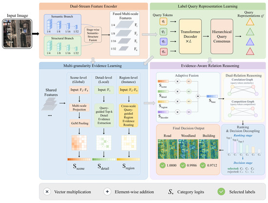
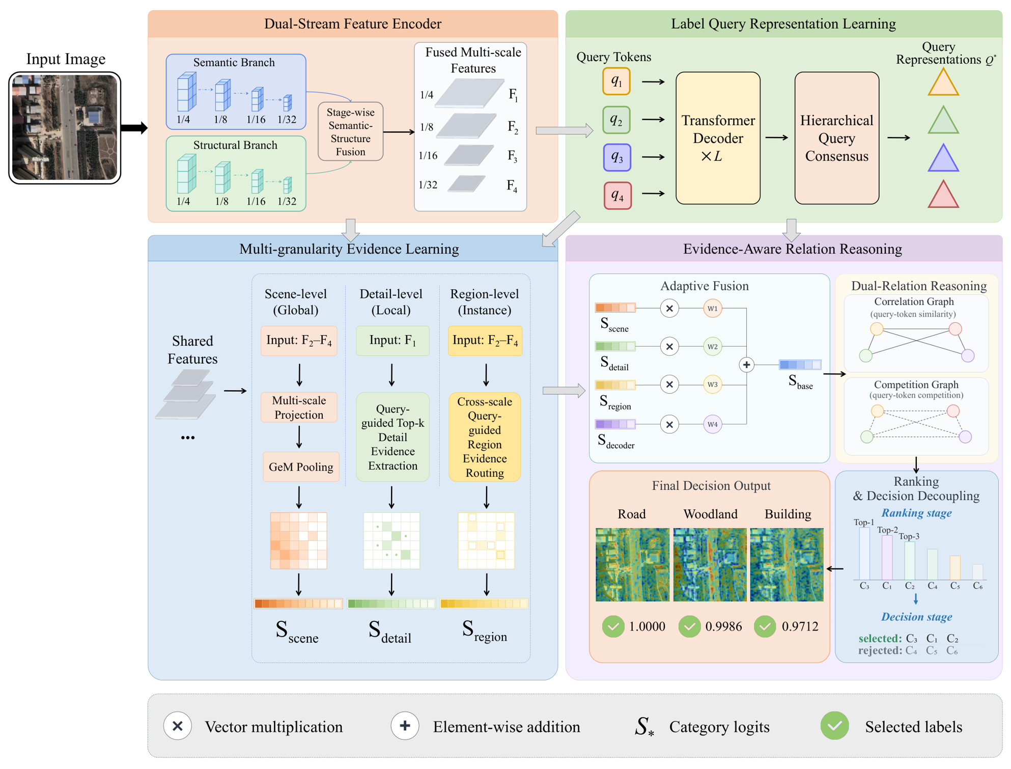
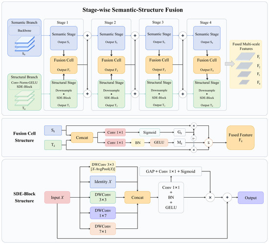
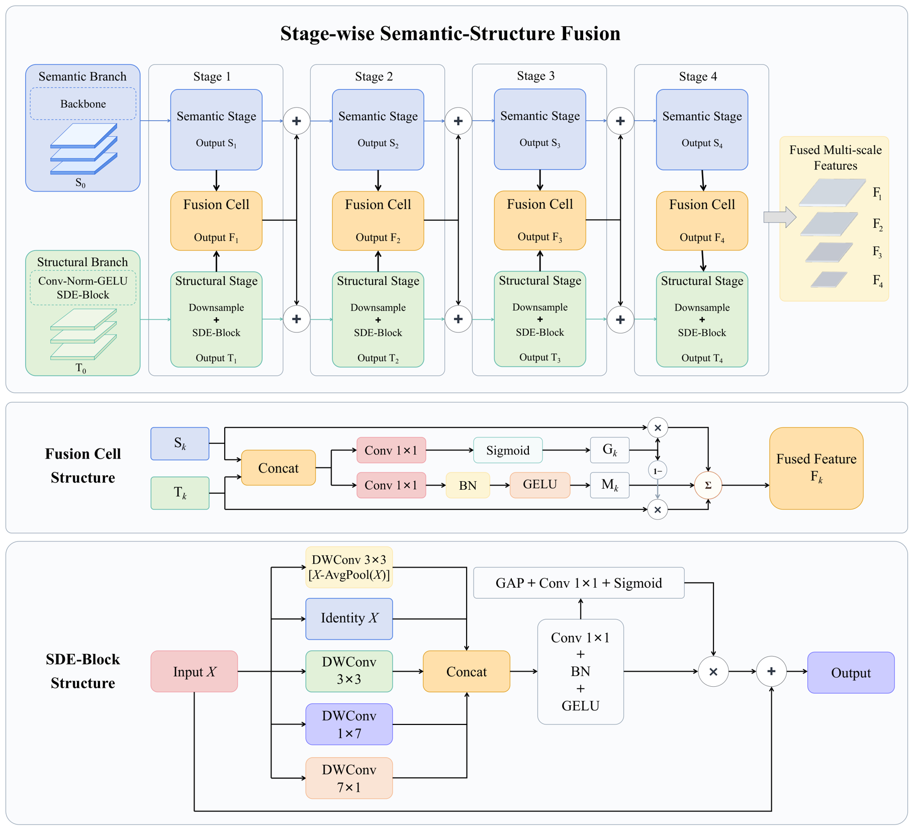
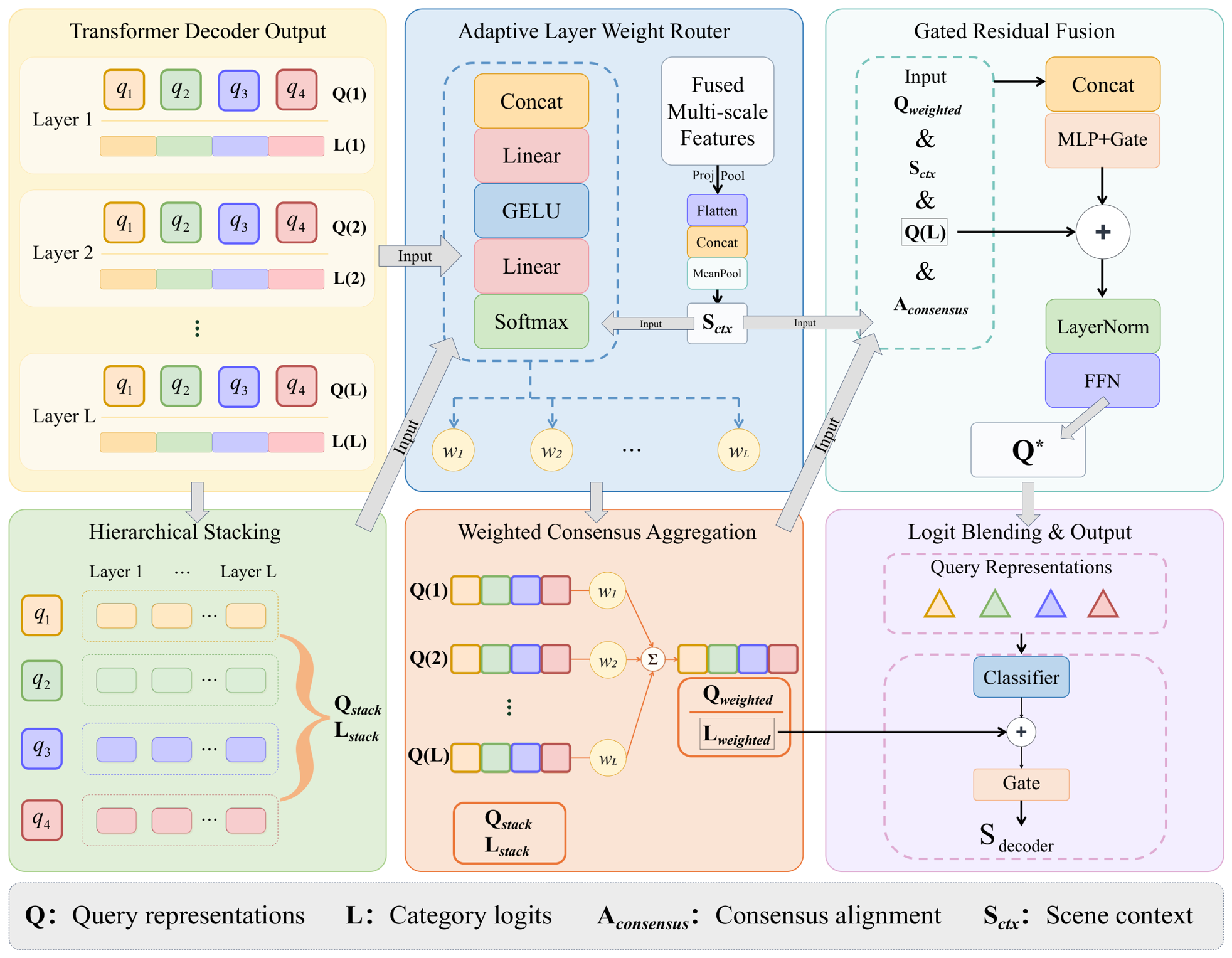
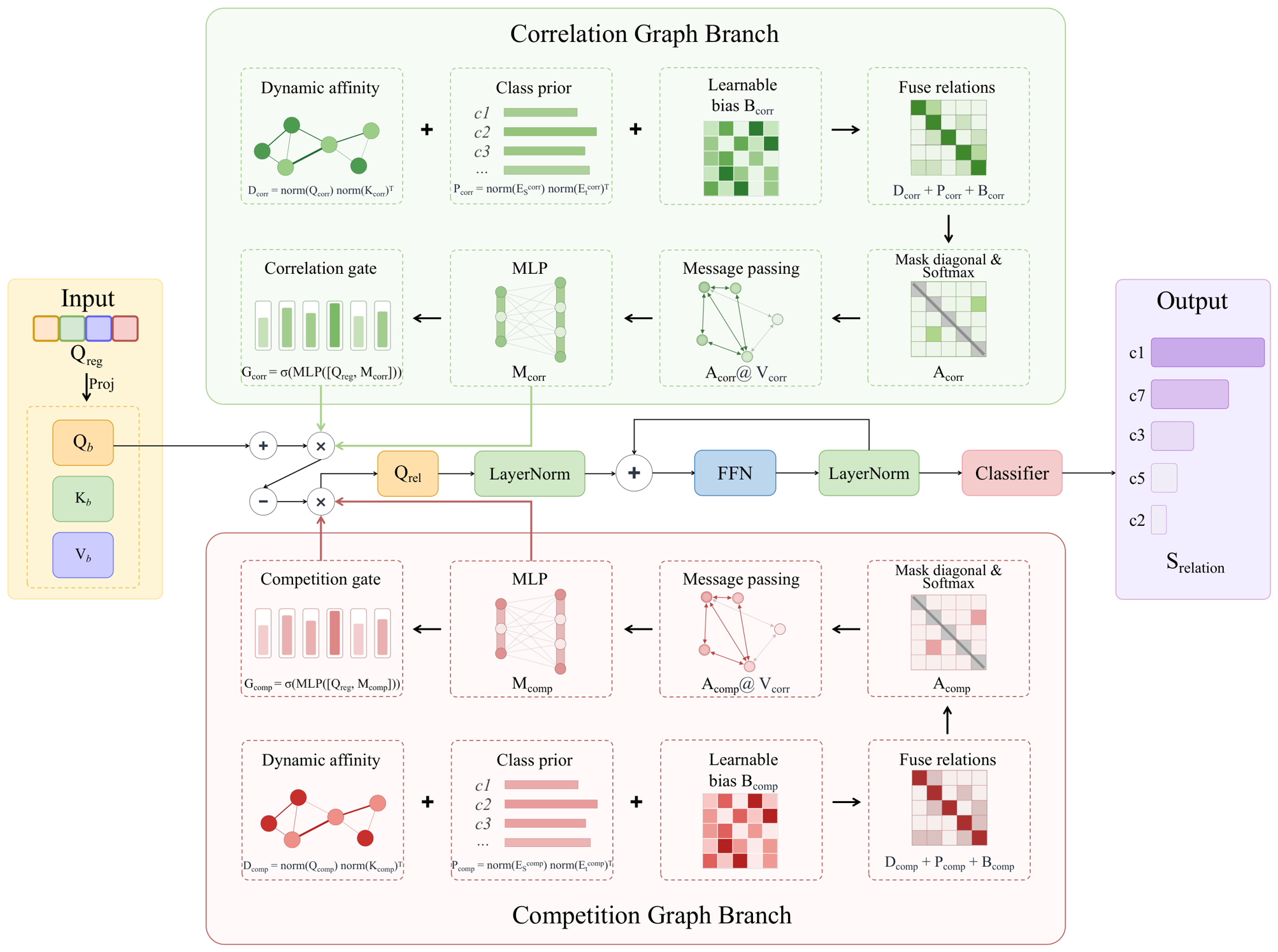
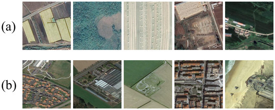
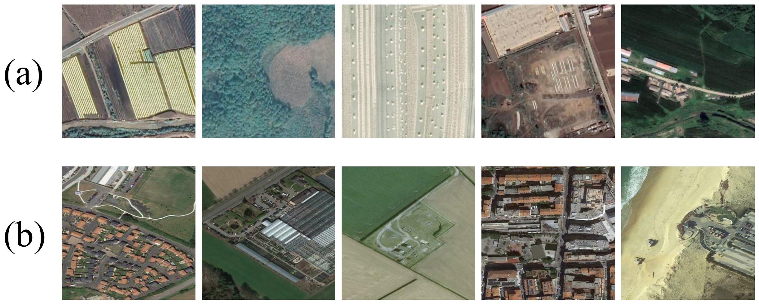
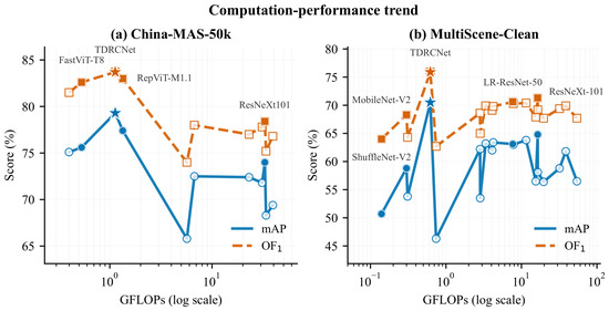
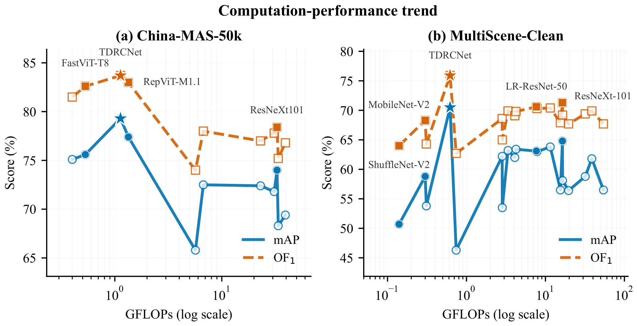
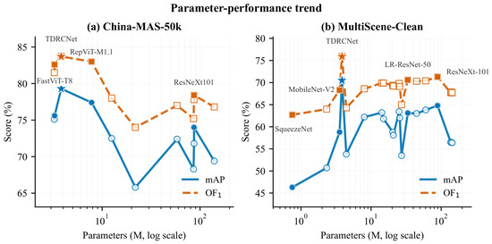
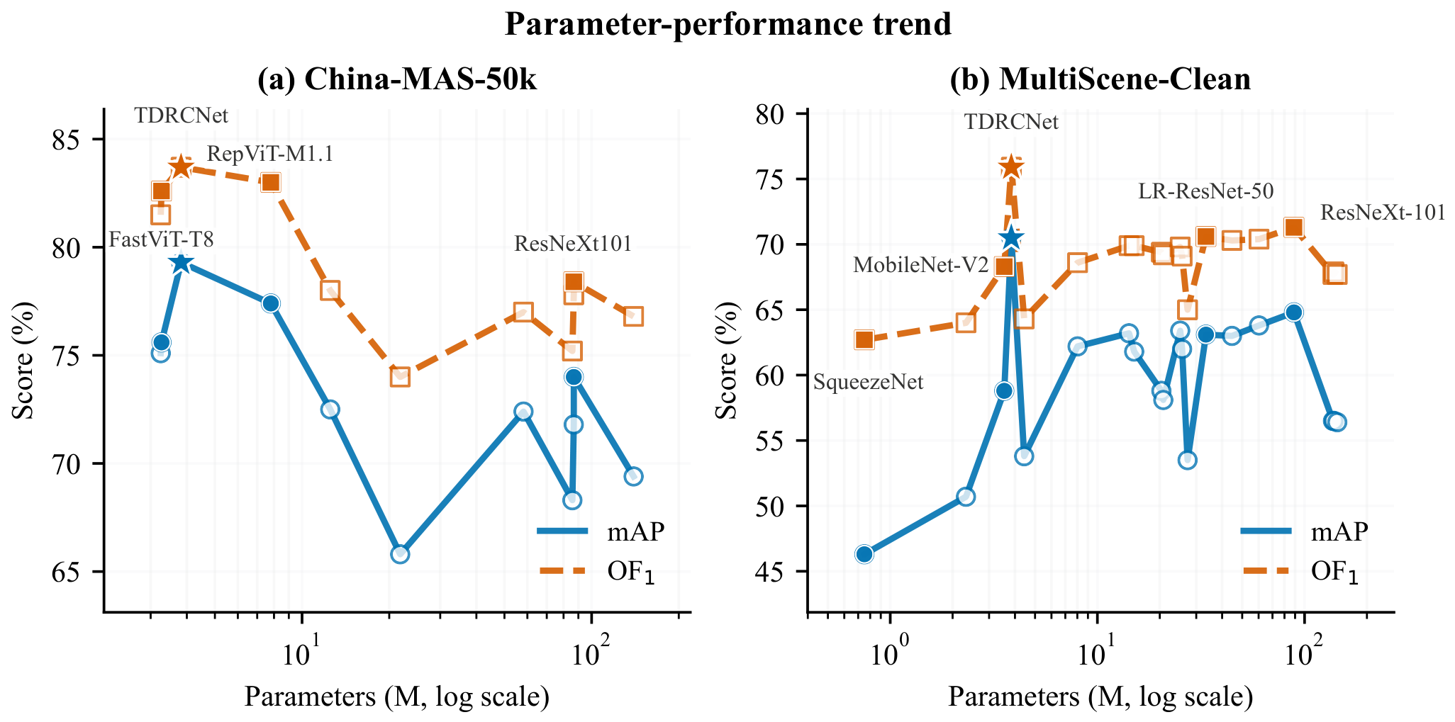
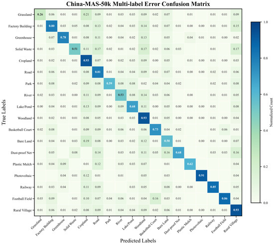
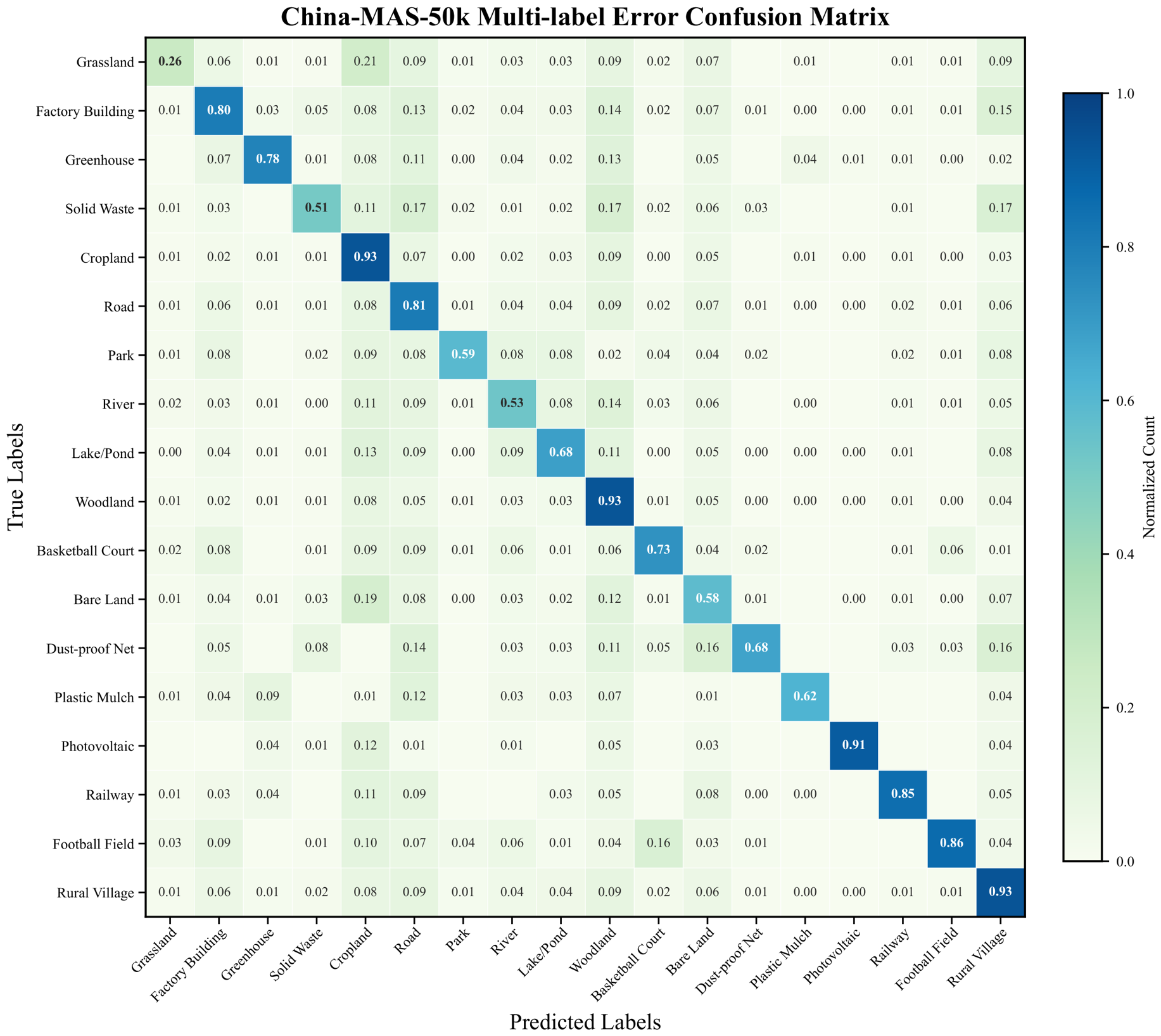
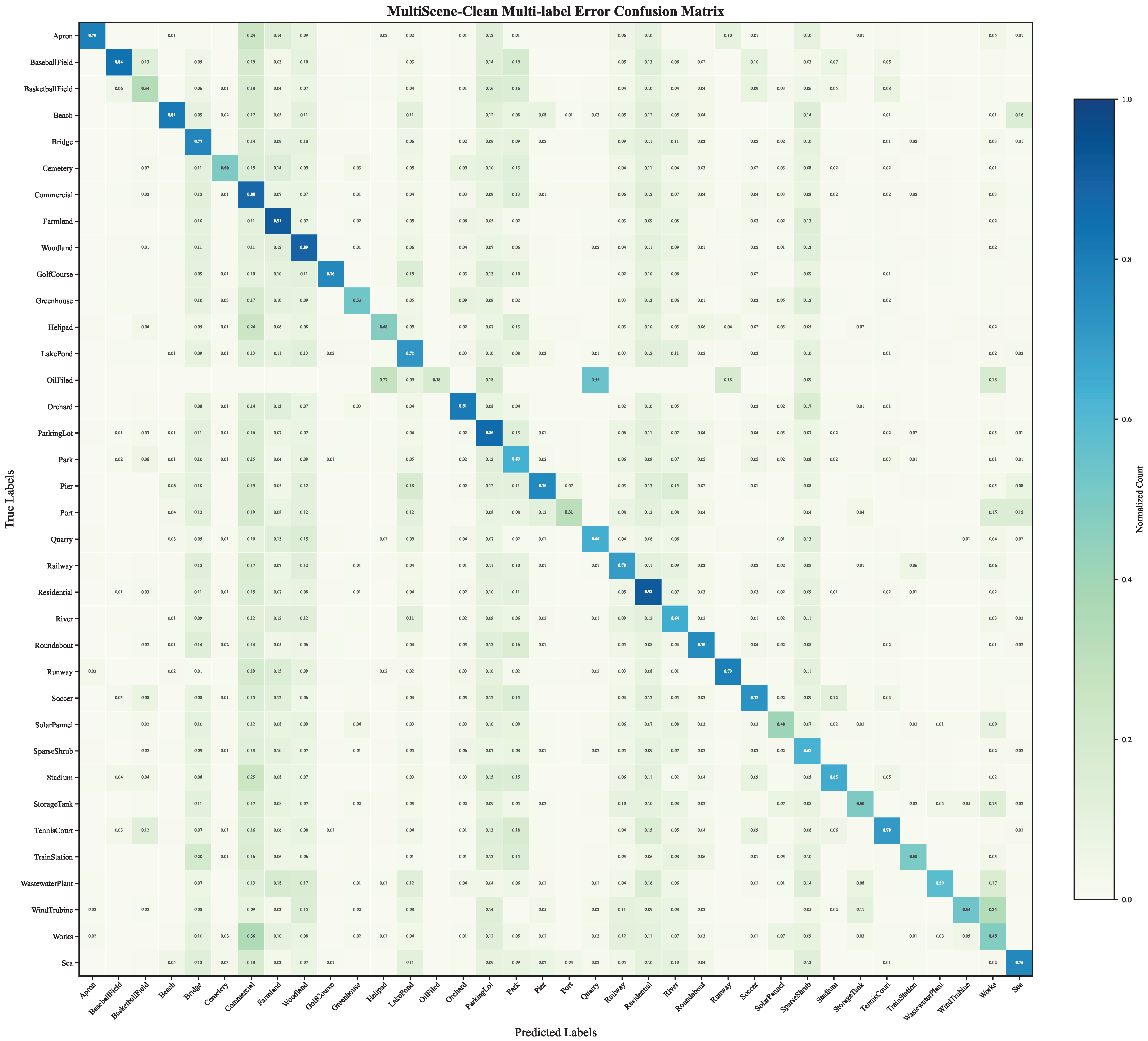
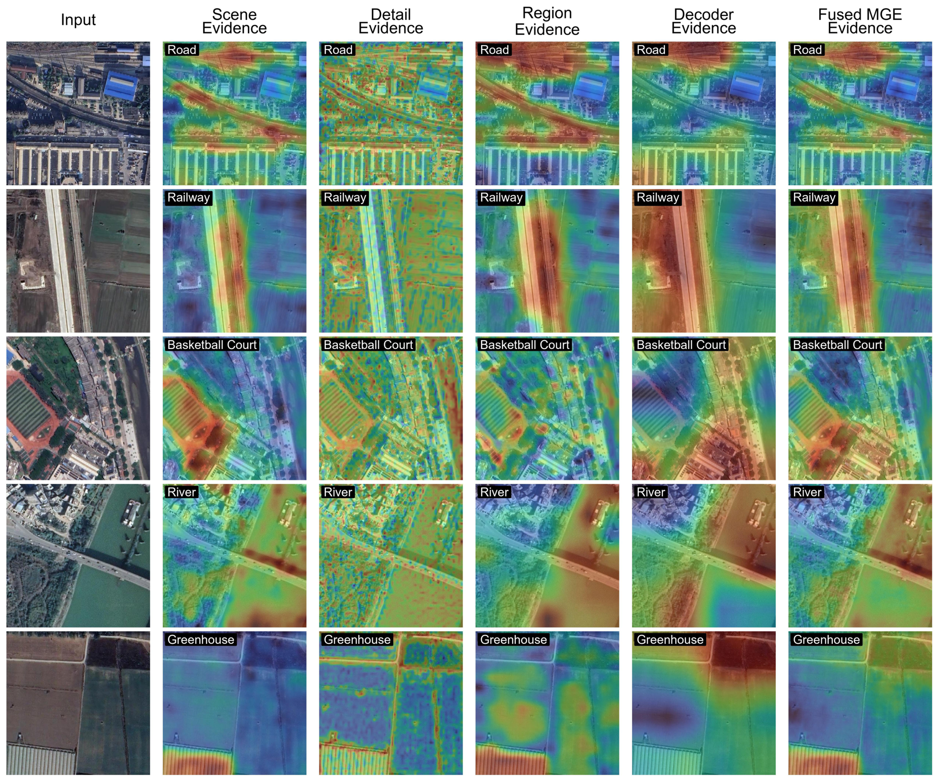
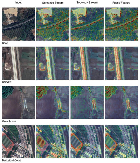
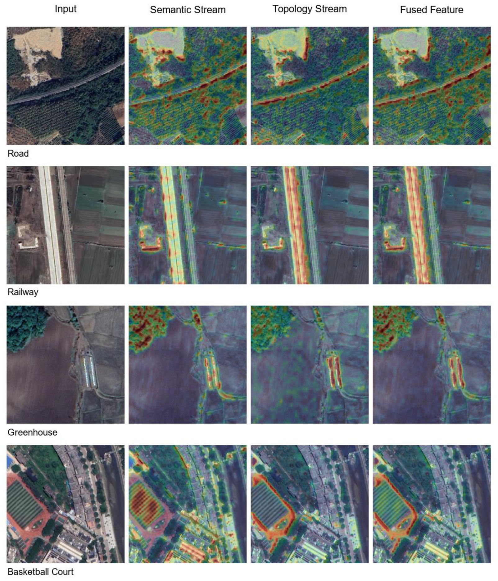
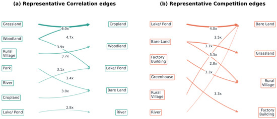
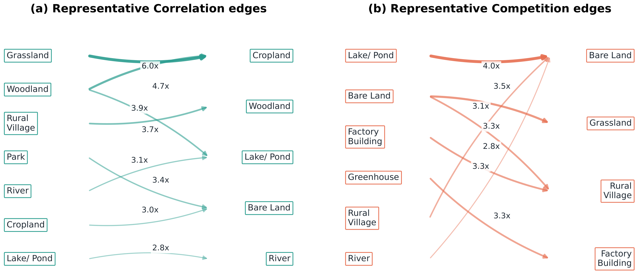

Disclaimer/Publisher’s Note: The statements, opinions and data contained in all publications are solely those of the individual author(s) and contributor(s) and not of MDPI and/or the editor(s). MDPI and/or the editor(s) disclaim responsibility for any injury to people or property resulting from any ideas, methods, instructions or products referred to in the content. |
© 2026 by the authors. Licensee MDPI, Basel, Switzerland. This article is an open access article distributed under the terms and conditions of the Creative Commons Attribution (CC BY) license.