Minimizing Peak Sidelobe Level in MIMO-SAR Waveform Design Using a 1.5-Entmax Sparse Loss

Highlights

What are the main findings?

• A 1.5-entmax sparse loss function is proposed for a MIMO-SAR orthogonal waveform design that achieves the lowest peak sidelobe level (PSL) across all evaluated waveform sizes and approaches the Levenshtein lower bound without any loss-function hyperparameter tuning.
• A GPU-accelerated, deep learning-based optimization framework with a custom analytical Jacobian operator reduces computation time by approximately two orders of magnitude compared with state-of-the-art methods in large-scale waveform-design scenarios ($M=128$, $N=1024$).

What are the implications of the main findings?

• The strict sparse-truncation mechanism eliminates gradient noise arising from low-energy sidelobes, thereby suppressing range sidelobes and azimuth ambiguities in MIMO-SAR imagery and improving the detectability of weak targets near strong scatterers.
• The rapid convergence and GPU-parallel scalability of the proposed framework establish its engineering viability for real-time orthogonal waveform synthesis in next-generation, large-scale MIMO-SAR Earth-observation systems.

Abstract

The peak sidelobe level (PSL) of an orthogonal waveform set directly governs the range and azimuth ambiguities of synthetic aperture radar (SAR) images and is therefore a key figure of merit for the imaging quality of multiple-input multiple-output SAR (MIMO-SAR). Minimizing the PSL is an NP-hard problem with a non-differentiable objective, and existing approaches often suffer from high computational cost and limited scalability while achieving only suboptimal PSL suppression. We therefore propose a loss function built around the 1.5-entmax sparse transform, which is simultaneously differentiable, sparse, and adaptive. Analysis of its differentiability and derivation of its analytical gradient allow us to recast the NP-hard problem as a differentiable optimization problem that can be solved by well-established algorithms. Owing to the sparsity of the transform, the gradient is concentrated on the high-energy sidelobes, while the gradient contribution from low-energy sidelobes becomes exactly zero, removing the gradient noise contributed by low-energy sidelobes and yielding a lower PSL. To overcome the scale sensitivity of the 1.5-entmax function, the upper bound on the sidelobe magnitude is used to normalize the input, which makes the threshold adaptive and removes the need for additional loss-function hyperparameter tuning across waveform-design tasks of different sizes. To further improve computational efficiency, we combine gradient descent with a deep learning framework: the waveform phases are treated as the learnable parameters of a neural network-like model, thereby yielding a back-propagation-based optimization framework with graphics processing unit (GPU) parallelism. The algorithm is implemented for parallel execution on GPU, and the gradient is computed efficiently through the network’s automatic differentiation in conjunction with a custom analytical-gradient operator, leading to a substantial increase in computational speed. Without the need for the manual tuning of loss-function hyperparameters, the proposed algorithm achieves the lowest PSL across waveform sets of various sizes and reduces computation time by approximately two orders of magnitude in large-scale settings.

1. Introduction

Synthetic aperture radar (SAR), with its all-day, all-weather Earth-observation capability, has been widely used in terrain mapping, disaster monitoring, ocean remote sensing, and military reconnaissance [1,2,3]. As Earth-observation missions demand ever wider swaths and higher resolutions, conventional SAR systems face an inherent trade-off between swath width and azimuth resolution [4]. Multiple-input multiple-output SAR (MIMO-SAR) can effectively increase the number of equivalent phase centers by transmitting mutually orthogonal waveforms, thereby improving azimuth resolution without sacrificing swath width [5,6]. In MIMO-SAR systems, the orthogonality of the waveform set has a direct impact on image quality: the auto-correlation sidelobe level affects the range point spread function (PSF), while cross-correlation components introduce inter-channel interference that is equivalent to azimuth ambiguity, severely degrading image contrast and the detectability of weak targets [7,8,9,10]. The design of orthogonal waveform sets with low auto-correlation sidelobes and low cross-correlation sidelobes is therefore a fundamental problem in MIMO-SAR signal processing.

Two key metrics characterize waveform orthogonality: the integrated sidelobe level (ISL) and the peak sidelobe level (PSL). The PSL directly reflects the worst sidelobe interference in SAR images and determines the extent to which strong scatterers mask nearby weak targets; it is therefore the constraint of primary engineering interest [11,12]. Early studies focused mainly on ISL minimization because of its tractable quadratic structure. Methods such as Cyclic Algorithm New (CAN) [13,14], majorization–minimization (MM) [15,16], alternating direction method of multipliers (ADMM) [17], and deep unfolding networks [18] can approach the theoretical lower bound on the ISL. However, low-ISL waveforms may still exhibit a high PSL, which compromises the detection of weak targets.

To suppress the PSL, several studies optimize it directly. The MM-based PSL minimizer constructs a surrogate function for the PSL and solves it efficiently using the fast Fourier transform (FFT), achieving monotonic descent [19].

The minimax method based on a primal–dual framework and the Proximal Minimax Method (PMM) embed the $L_{\infty }$-norm constraint directly into the augmented Lagrangian, providing strong PSL suppression [20,21]. Other works combine alternating minimization with a Lagrangian dual lower bound [22]. These methods, however, perform high-dimensional matrix operations at every iteration, which incur substantial computational overhead when the number of waveforms M and the code length N are large, limiting their applicability in large-scale scenarios.

Another common approach is to construct a joint objective by linearly combining PSL and ISL with appropriate weights. Examples include the coordinate-descent framework [23], the weighted-ISL MM method [24], WeBEST-v [25], a vectorized block-coordinate descent method based on Block Successive Upper-bound Minimization (BSUM) with an $L_p$-norm surrogate, the joint MM–ADMM framework [26], and the Block Iterative Shrinkage-Thresholding (BiST) algorithm based on block-coordinate descent [27].

All of these methods strike a flexible compromise between PSL and ISL by tuning the weighting coefficients. The Con method, which uses a residual network to perform weighted unsupervised optimization of PSL and ISL, also yields relatively low PSL values [28]. A common drawback of these approaches is that the weights must be re-tuned for each waveform size without theoretical guidance, and the weighted formulation itself does not address the non-differentiability of the PSL.

A widely adopted route to differentiability is to introduce an $L_p$-norm: with $p=2$, the objective reduces to the ISL, while, as $p\to \infty$, it approaches the PSL. Representative algorithms include the p-MM method, which successively solves low-order surrogate subproblems within an MM framework to approximate PSL minimization [29], and WeBEST-v, which performs vectorized block-coordinate descent based on BSUM [25]. Riemannian manifold approaches model the problem on the complex circular-product manifold and directly optimize the $L_p$-norm via trust-region methods [30,31]. $L_p$-norm-based algorithms have also been extended to Doppler-tolerant scenarios [32], to a unified analysis of high-order norms [33], and to the joint design of waveforms and mismatched filters [34]. A common drawback of these methods is their strong dependence on the choice of p: different algorithms exhibit different sensitivities to p. If p is too small, the objective degenerates toward the ISL, and peak suppression is insufficient; if p is too large, high-order exponentiation causes gradient explosion or numerical overflow. Moreover, the optimal p varies with the waveform size and must be re-tuned in each case, which limits their practical applicability across different waveform sizes.

Some existing methods approximate the non-differentiable maximum operator with a smooth surrogate so that it can be incorporated directly into a gradient-based framework. One approach uses the log-sum-exp (LSE) function to smoothly approximate the PSL and combines it with the Adam optimizer, with good empirical results [35]. An iterative neural network method based on the Mellowmax operator likewise provides a smooth approximation of the PSL and obtains low PSL values [36]. The two smoothing functions belong to the same family and are mathematically equivalent. Such methods scale well to large problems, but they suffer from two structural shortcomings. First, the smoothing parameter has to be tuned manually; in the LSE, for example, too small a t causes gradient oscillations, whereas too large a t degrades the approximation accuracy. Second, when the total number of sidelobes reaches hundreds of thousands, the accumulated gradient contribution from a vast number of low-energy sidelobes—henceforth termed gradient noise—masks the gradient signal of the high-energy sidelobes, slowing convergence and preventing further reduction in the PSL.

In summary, in pursuit of a differentiable surrogate for the PSL that is amenable to optimization, the global power weighting of the $L_p$-norm, the softmax-style soft weighting of the LSE, and linear weighted combinations all distribute the weights across all sidelobes. To further reduce the PSL, however, the optimization weight should be concentrated on the high-energy sidelobes, with the ideal weight on low-energy sidelobes being exactly zero—in other words, the weights should be sparse. An ideal PSL objective should therefore satisfy the following four properties simultaneously: (1) focus only on high-energy sidelobes so as to effectively reduce the PSL; (2) impose strict truncation on low-energy sidelobes to suppress the gradient noise they would otherwise inject; (3) maintain differentiability with respect to the phase parameters to support efficient gradient-based optimization; and (4) adapt well to different waveform sizes without the need for loss-function hyperparameter tuning.

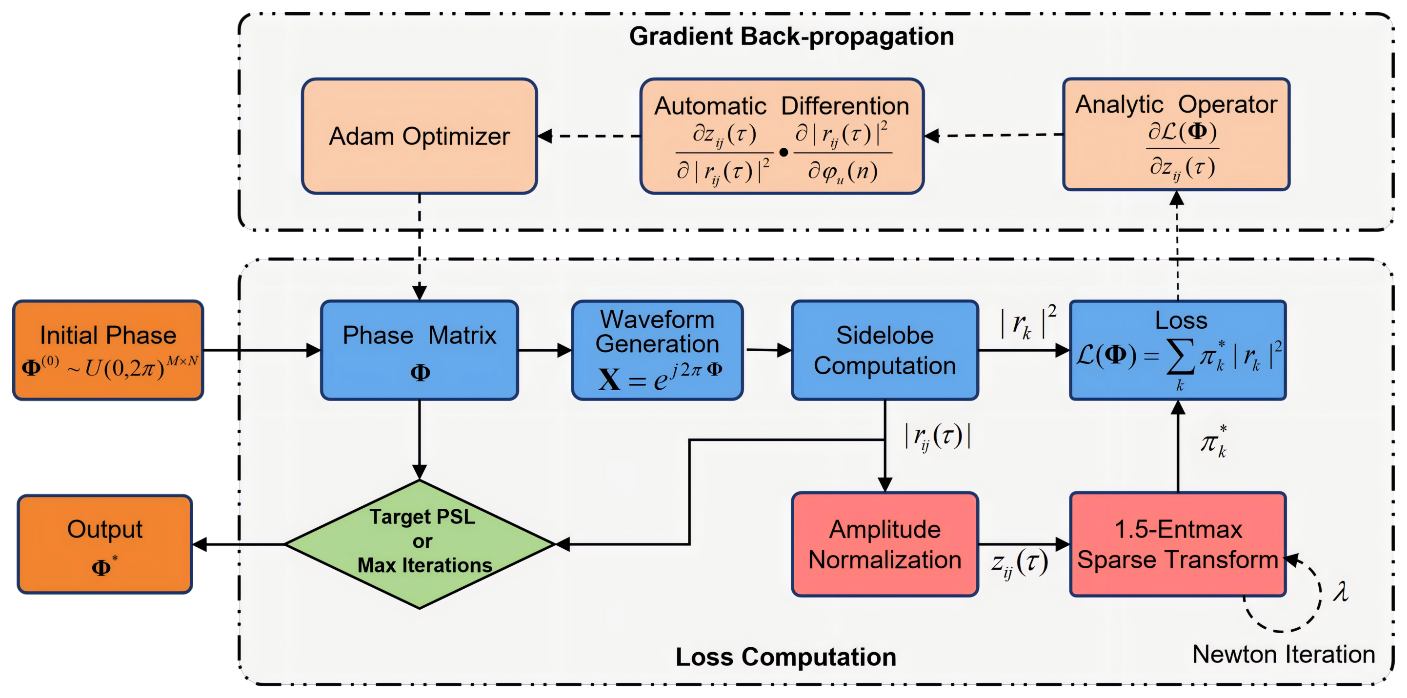
Motivated by these requirements, this paper proposes a loss function based on the 1.5-entmax sparse transform [37] as a sidelobe weighting function. While remaining differentiable, the proposed loss adaptively concentrates the optimization on the high-energy sidelobes and strictly truncates low-energy sidelobes, preventing them from accumulating gradient noise. To avoid the construction of surrogate functions and the heavy computations involved in conventional algorithms, we develop an optimization framework that leverages GPU-accelerated automatic differentiation and a custom analytical-gradient operator to minimize the proposed loss efficiently. The main contributions of this paper are summarized as follows:

• The 1.5-entmax function is introduced into MIMO-SAR waveform design. By exploiting the sparsity of its output, the optimization automatically focuses on high-energy sidelobes and strictly truncates low-energy ones. This eliminates gradient noise at its source, removing the perturbation that arises in existing smooth approximations where all sidelobes participate in the gradient, and yields lower PSL values.
• To address the inherent scale sensitivity of the 1.5-entmax function, a normalization preprocessing step based on the theoretical upper bound of the sidelobe is introduced. This allows the truncation threshold $\lambda$ to adapt automatically to the relative distribution of sidelobes. A rigorous proof of differentiability and a closed-form analytical gradient are also provided, which together facilitate efficient and stable convergence.
• The proposed loss function is embedded into a deep learning optimization framework that combines GPU-accelerated automatic differentiation with a custom analytical-gradient operator. For the sparse-truncation step, an analytical Jacobian operator that bypasses the computation-graph expansion of automatic differentiation is constructed, keeping the per-iteration complexity at $\mathcal{O}(M^{2}NlogN)$.
• Extensive simulation experiments confirm that the proposed method attains state-of-the-art PSL values for all waveform sizes considered and consistently approaches the Levenshtein lower bound. In large-scale scenarios, it achieves a speedup of approximately two orders of magnitude over existing state-of-the-art methods, demonstrating its potential for online waveform design.

The remainder of this paper is organized as follows: Section 2 establishes the signal model and defines the performance metrics. Section 3 details the design and theoretical analysis of the proposed loss function. Section 4 describes the deep learning-based optimization framework. Section 5 presents simulation experiments under various scenarios and compares the proposed method with representative baselines. Section 7 concludes the paper and discusses directions for future work.

2. Problem Formulation

2.1. Signal Model

Orthogonality in MIMO-SAR can be realized in three ways: time-division multiplexing (TDM), frequency-division multiplexing (FDM), and code-division multiplexing (CDM). TDM waveforms increase the total pulse duration and thus substantially reduce the unambiguous swath, whereas FDM waveforms require additional mixing circuits, which degrade signal coherence and increase system cost [38]. In MIMO-SAR, CDM offers a larger time–bandwidth product and stronger interference rejection; this paper therefore adopts phase-coded waveforms.

Consider a one-dimensional, uniform, linear array with M transmit and M receive elements. The set of baseband signals is denoted by $\{x_1\left(t\right),x_2\left(t\right),\dots ,x_M\left(t\right)\}$, where $x_u\left(t\right)$ is the baseband waveform of the u-th antenna. The signal transmitted by the u-th antenna element is expressed as

$$s_u\left(t\right)=\sqrt{{\displaystyle \frac{E}{M}}}{x}_u\left(t\right)rect\left({\displaystyle \frac{t}{T}}\right),$$

(1)

where E is the total transmitted energy, M is the number of transmit elements, $x_u\left(t\right)$ is the baseband signal of the u-th antenna, T is the pulse duration, and $rect(·)$ denotes the unit rectangular pulse. The baseband waveform can be written as

$$x_u\left(t\right)={\displaystyle \sum _{n=0}^{N-1}}{x}_u\left(n\right)rect\left({\displaystyle \frac{t-n{T}_c}{T_c}}\right),$$

(2)

where $T_c$ is the chip duration and N is the number of chips. The N chips can be stacked into a vector

$${\mathit{x}}_u={\left[x_u\left(0\right),x_u\left(1\right),\dots ,x_u(N-1)\right]}^{\mathrm{T}}.$$

(3)

The n-th chip of the u-th waveform has constant modulus, $x_u\left(n\right)=exp\left(\mathrm{j}{\phi }_u\left(n\right)\right)$, with ${\phi }_u\left(n\right)\in [0,2\pi )$. The phase-coded signals from the M transmit elements are stacked row-wise into the matrix

$$\mathit{X}={[{\mathit{x}}_1,{\mathit{x}}_2,\dots ,{\mathit{x}}_M]}^{\mathrm{T}}\in {\mathbb{C}}^{M\times N}.$$

(4)

Modern radar receivers typically perform discrete digital signal processing, and correlation values at non-integer delays can be approximated by linear interpolation between adjacent samples [39]. The discrete cross-correlation function is therefore written as

$$r_{ij}\left(\tau \right)={\displaystyle \sum _{n=0}^{N-1}}{x}_i^{*}\left(n\right)x_j(n+\tau ),\tau =-(N-1),\dots ,N-1,$$

(5)

where equivalently, each finite-length sequence is extended by the zero-padding convention $x_u\left(n\right)=0$ for $n\notin \{0,1,\dots ,N-1\}$, so that the summation effectively runs only over the overlapping support $n\in [max(0,-\tau ),min(N-1,N-1-\tau \left)\right]$.

For an ideally orthogonal waveform set, the auto-correlation function is nonzero only at zero delay, and all auto-correlation sidelobes and cross-correlation components vanish. Accordingly, the orthogonality of a waveform set can be quantified by performance metrics such as the integrated sidelobe level (ISL) and the peak sidelobe level (PSL).

2.2. Performance Metrics

In practical radar applications, the peak sidelobe level strongly affects target detection performance. Reducing the PSL lowers the false-alarm rate and improves detection reliability, thereby enhancing the overall system performance. We therefore aim to minimize the PSL, suppressing auto-correlation sidelobes and inter-waveform interference. The PSL may originate either from the auto-correlation peak sidelobe level (${\mathrm{PSL}}_{\mathrm{A}}$) or from the cross-correlation peak sidelobe level (${\mathrm{PSL}}_{\mathrm{C}}$); we therefore define the following metrics.

The auto-correlation peak sidelobe level ${\mathrm{PSL}}_{\mathrm{A}}$ is the largest magnitude among all auto-correlation values at nonzero delays:

$${\mathrm{PSL}}_{\mathrm{A}}=\underset{i,\tau \ne 0}{max}{\left|r_{ii}\left(\tau \right)\right|}^2.$$

(6)

The cross-correlation peak sidelobe level ${\mathrm{PSL}}_{\mathrm{C}}$ is the largest magnitude among all cross-correlation sidelobes:

$${\mathrm{PSL}}_{\mathrm{C}}=\underset{i\ne j,\tau }{max}{\left|r_{ij}\left(\tau \right)\right|}^2.$$

(7)

The global peak sidelobe level $\mathrm{PSL}$ is the larger of the two:

$$\mathrm{PSL}=max\left\{\underset{i,\tau \ne 0}{max}|r_{ii}{\left(\tau \right)|}^2,\underset{i\ne j,\tau }{max}{\left|r_{ij}\left(\tau \right)\right|}^2\right\}.$$

(8)

The PSL is a key design criterion for evaluating and optimizing the orthogonality and correlation properties of MIMO-SAR waveforms. Under the constant-modulus constraint, the optimization problem can be formulated as

$$\begin{array}{c}{\displaystyle \underset{\mathit{X}}{min}}\mathrm{PSL}\\ \mathrm{s}.\mathrm{t}.|x_u\left(n\right)|=1,\forall u,n.\end{array}$$

(9)

The ultimate goal is to minimize the $\mathrm{PSL}$; however, the $\mathrm{PSL}$ is a non-differentiable maximum function, and direct optimization often exhibits oscillatory behavior, hindering convergence to a sufficiently low value.

3. Design and Differentiability Analysis of the Loss Function

To address the non-differentiability of the $\mathrm{PSL}$ noted at the end of Section 2 and the gradient-noise issue raised in Section 1, this section constructs a loss function based on the 1.5-entmax transform. We first analyze the properties of the entmax transform and discuss the choice of the parameter $\alpha$. We then identify the issues caused by its scale sensitivity and present a remedy. On this basis, the loss function is defined, and a rigorous proof of differentiability together with a closed-form expression for the analytical gradient is provided.

3.1. Entmax Transform and Parameter Selection

Smoothing the PSL essentially balances the sidelobe weights between PSL and ISL. The LSE and Mellowmax operators currently used for smoothing adopt a softmax-style weight distribution. Although this makes the PSL differentiable, it also assigns positive weights to low-energy sidelobes and thereby introduces gradient noise. Ideally, the weights should also be sparse, so that the weights of low-energy sidelobes are exactly zero and only the high-energy sidelobes have nonzero weights.

Peters et al. [37] unified the softmax function used for smoothing and the sparsemax function used in sparse attention into the $\alpha$-entmax family. Entmax can be both differentiable and sparse, so we adopt it to address the differentiability and gradient-noise issues simultaneously. The $\alpha$-entmax is the solution of a convex optimization problem regularized by Tsallis $\alpha$-entropy:

$${\mathit{\pi }}^{*}={\displaystyle \underset{\mathit{\pi }\in {\Delta }^{K-1}}{arg\; max}}\langle \mathit{\pi },\mathit{z}\rangle +H_{\alpha }^{\mathrm{T}}\left(\mathit{\pi }\right),$$

(10)

where ${\Delta }^{K-1}$ is the K-dimensional probability simplex, $\mathit{z}\in {\mathbb{R}}^K$ is the input vector, and the Tsallis $\alpha$-entropy is defined as

$$H_{\alpha }^{\mathrm{T}}\left(\mathit{\pi }\right)={\displaystyle \frac{1}{\alpha (\alpha -1)}}{\displaystyle \sum _{k=1}^K}\left({\pi }_k-{\pi }_k^{\alpha }\right).$$

(11)

Forming the Lagrangian of this problem and solving the Karush–Kuhn–Tucker (KKT) conditions yield a unified closed-form expression for the optimal solution:

$${\pi }_k^{*}\left(\mathit{z}\right)={\left[(\alpha -1)z_k-\lambda \right]}_{+}^{1/(\alpha -1)},$$

(12)

where ${\left[a\right]}_{+}=max\{a,0\}$ is the positive-part operator and the threshold $\lambda$ is uniquely determined by the normalization constraint ${\sum }_k{\pi }_k^{*}=1$. The parameter $\alpha$ is a real number greater than one, and its value controls the sparsity and differentiability of the output. To avoid hardware-inefficient fractional root extractions during repeated evaluations of Equation (12), we restrict $1/(\alpha -1)$ to be a positive integer q, giving $\alpha =1+1/q\in (1,2)$. The value $q=2$ yields the largest such $\alpha$, namely, $\alpha =1.5$, and Equation (12) simplifies to

$${\pi }_k^{*}={\left[{\displaystyle \frac{z_k}{2}}-\lambda \right]}_{+}^2.$$

(13)

Three representative cases arise within the range $1\le \alpha \le 2$.

• When $\alpha =1$, we recover the softmax function, whose output ${\pi }_k^{*}={\displaystyle \frac{{\mathrm{e}}^{z_k}}{{\sum }_j{\mathrm{e}}^{z_j}}}$ is strictly positive in every component; low-energy sidelobes always receive nonzero weights, so the output is not sparse, although it is $C^{\infty }$ smooth.
• When $\alpha =2$, we recover the sparsemax function, which simplifies to the linear truncation ${\pi }_k^{*}={\left[z_k-\lambda \right]}_{+}$. The weights of sidelobes below the threshold are zero, yielding strong sparsity, but the function is not differentiable at the truncation point $z_k=\lambda$.
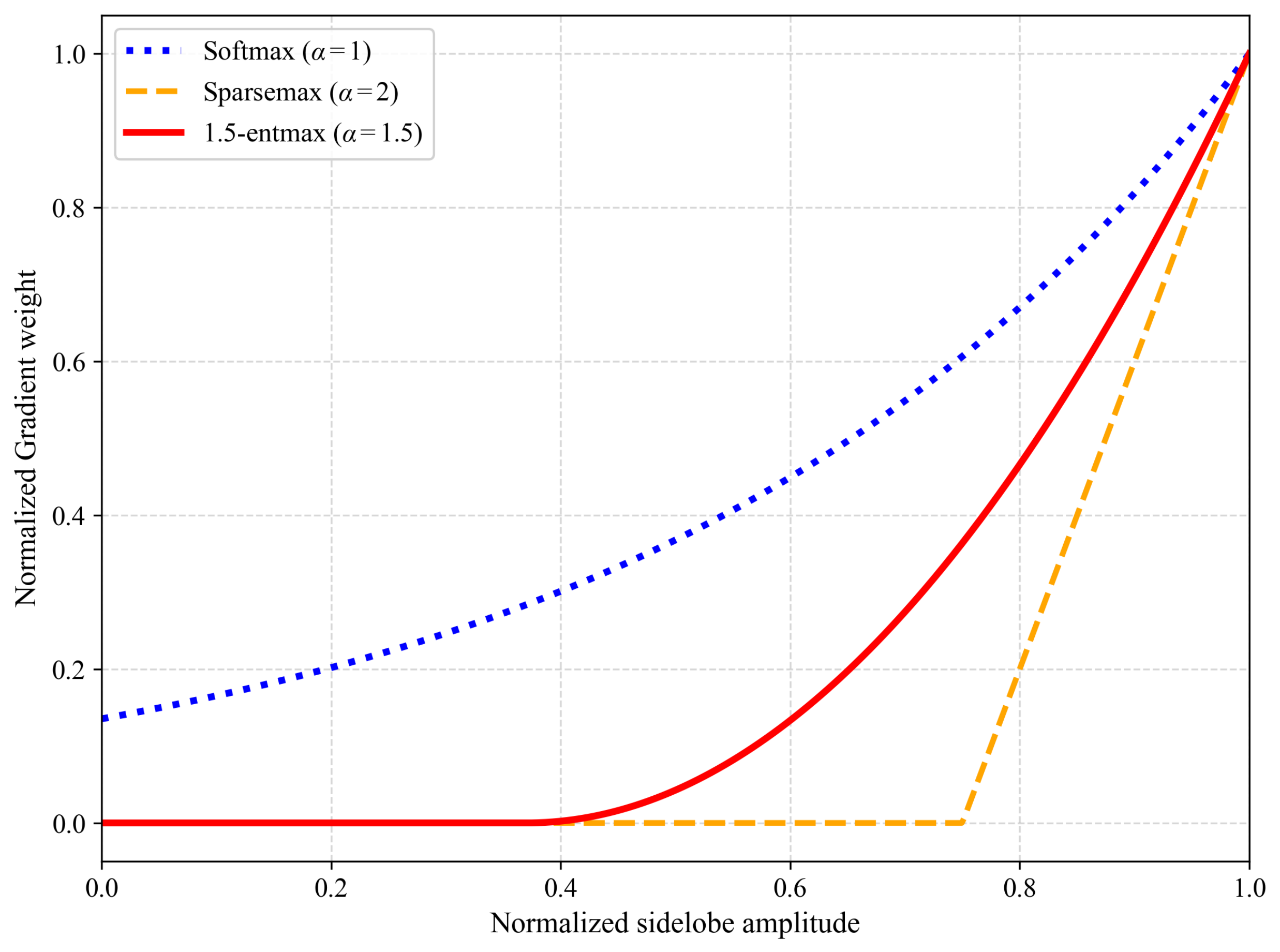
• When $1<\alpha <2$, the $\alpha$-entmax is both sparse and differentiable: larger $\alpha$ yields stronger sparsity, while smaller $\alpha$ yields a smoother profile. The choice $\alpha =1.5$ is the largest value that avoids root-extraction operations.

This choice filters out gradient noise effectively while maintaining moderate sparsity, avoiding the loss of critical information that overly aggressive truncation would entail.

Figure 1 shows the normalized gradient weights as a function of the sidelobe magnitude for the three values of $\alpha$. As can be seen, softmax still assigns nonzero weights in the low-energy region, sparsemax is non-differentiable at the threshold, and 1.5-entmax achieves both strict truncation and smoothness at the boundary.

Considering sparsity, differentiability, gradient noise, and computational complexity together, we build the loss function around the 1.5-entmax transform.

3.2. Scale Sensitivity and Normalization Preprocessing

Although the 1.5-entmax transform produces sparse weights, it is highly sensitive to the overall scale of the input vector. Let $\mathit{z}={[z_1,z_2,\dots ,z_K]}^{\mathrm{T}}$ denote the sidelobe vector and ${\mathit{\pi }}^{*}$ the weights produced by 1.5-entmax, with

$${\pi }_k^{*}={\left[{\displaystyle \frac{z_k}{2}}-\lambda \right]}_{+}^2,\sum _k{\pi }_k^{*}=1,$$

(14)

where the threshold $\lambda$ is uniquely determined by ${\sum }_k{\left[z_k/2-\lambda \right]}_{+}^2=1$. If the input is rescaled by a factor a ($a>0$, $a\ne 1$), so that ${\mathit{z}}^{\prime }=a\mathit{z}$, the new threshold ${\lambda }^{\prime }$ must satisfy

$$\sum _k{\left[{\displaystyle \frac{a{z}_k}{2}}-{\lambda }^{\prime }\right]}_{+}^2=1.$$

(15)

Setting ${\lambda }^{\prime }=a\lambda$ would make the left-hand side of Equation (15) equal to $a^2$, so the equality cannot hold; hence ${\lambda }^{\prime }\ne a\lambda$. This means that the magnitude and the threshold are not affected in the same way by rescaling, so the distribution of ${\pi }_k^{*}\left({\mathit{z}}^{\prime }\right)={\left[a{z}_k/2-{\lambda }^{\prime }\right]}_{+}^2$ generally differs in shape from the original ${\mathit{\pi }}^{*}\left(\mathit{z}\right)$. In other words, 1.5-entmax is not scale-invariant: proportionally rescaled inputs produce different weight allocations.

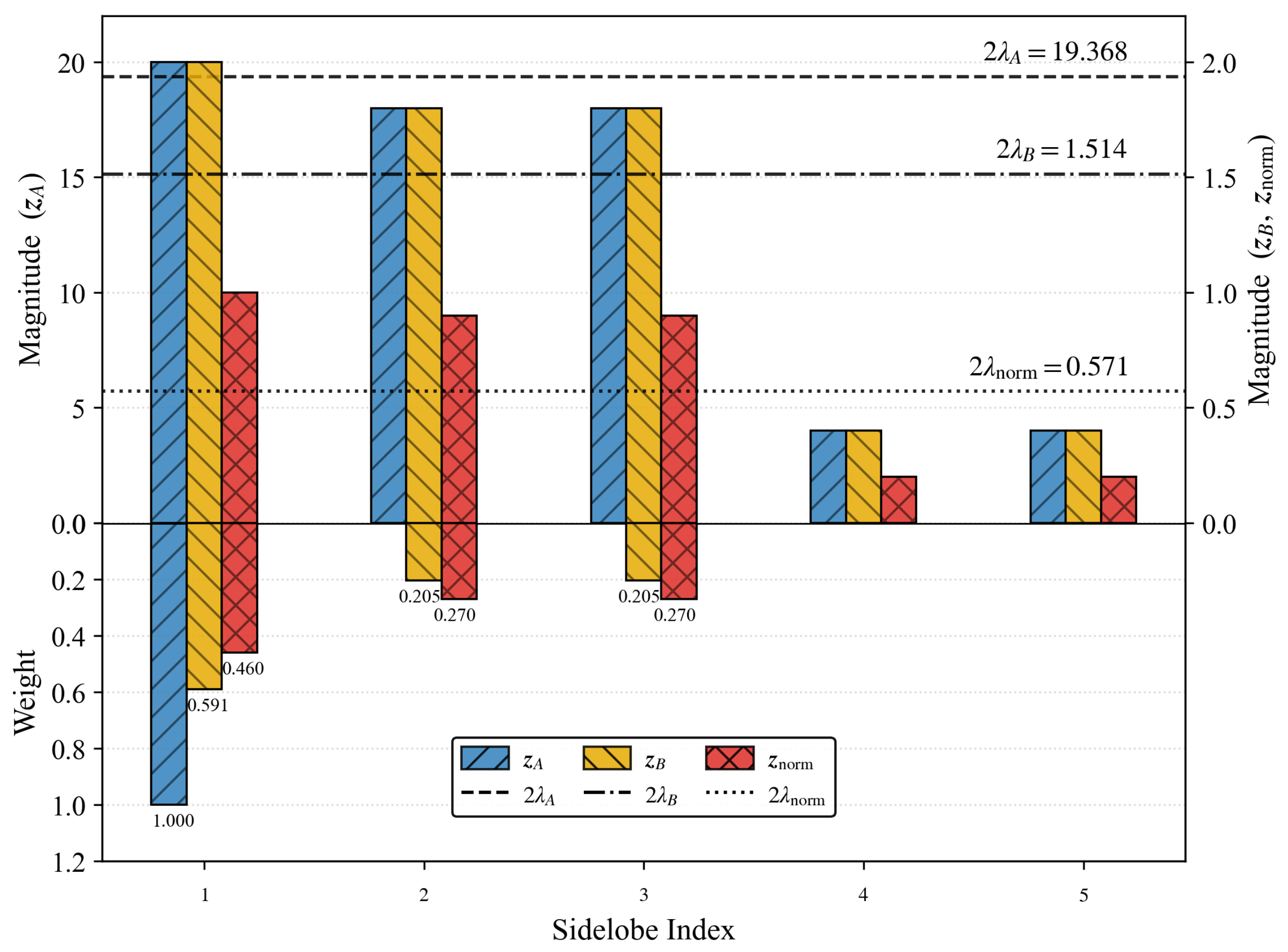
When M is fixed but N varies, two sets of sidelobes may have the same relative proportions but different absolute magnitudes. To illustrate the effect of scale sensitivity, consider the two similar sidelobe distributions ${\mathit{z}}_A=[20,18,18,4,4]$ and ${\mathit{z}}_B=[2,1.8,1.8,0.4,0.4]$: the relative proportions are identical, but the absolute magnitudes differ by a factor of ten. After applying the 1.5-entmax transform, Equation (14) produces different thresholds ${\lambda }_A$ and ${\lambda }_B$ and different weight distributions ${\mathit{\pi }}_A^{*}$ and ${\mathit{\pi }}_B^{*}$ (see Figure 2, where the upper panel shows the magnitudes and the lower panel shows the corresponding weights). For ${\mathit{z}}_A$, with the larger magnitudes, the threshold rises, the support shrinks, and almost all of the weight concentrates on the single largest sidelobe—a behavior that does not match the actual sidelobe distribution. For ${\mathit{z}}_B$, with smaller overall magnitudes, the threshold drops, the support enlarges, and the weights are more dispersed. Ideally, weight allocation should depend only on the relative sizes of the sidelobes and should not be perturbed by their absolute magnitudes.

To resolve this issue, we normalize all sidelobe magnitudes by their theoretical upper bound before applying the 1.5-entmax transform. For constant-modulus phase-coded waveforms, the Cauchy–Schwarz inequality yields

$$|r_{ij}\left(\tau \right)|=\left|\sum _n{x}_i^{*}\left(n\right)x_j(n+\tau )\right|\le N,$$

(16)

where equality holds if and only if $\tau =0$ and $x_j\left(n\right)=e^{\mathrm{j}\theta }{x}_i\left(n\right)$ (i.e., the two sequences are identical up to a constant phase). Hence N is a valid upper bound for all sidelobe magnitudes. Define the normalized magnitude

$$z_{ij}\left(\tau \right)={\displaystyle \frac{|r_{ij}\left(\tau \right)|}{N}}\in [0,1].$$

(17)

Because ${\mathit{z}}_A$ and ${\mathit{z}}_B$ share the same relative proportions, they map to the same normalized vector ${\mathit{z}}_{\mathrm{norm}}$. Applying the 1.5-entmax transform to ${\mathit{z}}_{\mathrm{norm}}$ yields the weight distribution ${\mathit{\pi }}_{\mathrm{norm}}^{*}$ shown in red in Figure 2. The normalized weight distribution is more reasonable, and lower sidelobes are also truncated. Once normalized, all sidelobe magnitudes are confined to the unit interval $[0,1]$; the absolute-magnitude information is removed, and the dynamic threshold $\lambda$ is determined solely by the relative sizes of the sidelobes, eliminating the influence of scale on weight allocation.

3.3. Loss Function and Threshold Computation

Feeding the normalized magnitudes $\mathit{z}\in {[0,1]}^K$ into the 1.5-entmax transform yields the sparse weight vector ${\mathit{\pi }}^{*}\in {\Delta }^{K-1}$, where

$$K=2M^{2}N-M^2-M$$

(18)

is the total number of sidelobes (including the nonzero-delay terms of the M auto-correlations and the $M(M-1)$ cross-correlation pairs). With ${\mathit{\pi }}^{*}$ as coefficients, the loss function is defined as

$$\mathcal{L}\left(\mathsf{\Phi }\right)={\displaystyle \sum _{k=1}^K}{\pi }_k^{*}·{\left|r_k\left(\mathsf{\Phi }\right)\right|}^2,$$

(19)

where the index k is a flattened linear index of the triple $(i,j,\tau )$, and k and $(i,j,\tau )$ are in one-to-one correspondence. This expression can equivalently be interpreted as the weighted expectation of the sidelobe powers under the sparse weights ${\mathit{\pi }}^{*}$. It has three key properties:

• Adaptive focusing. The weights ${\mathit{\pi }}^{*}$ are not fixed but are determined automatically by 1.5-entmax from the sidelobe distribution at each iteration. Higher-energy sidelobes receive larger weights and therefore stronger gradients.
• Strict truncation. Sidelobes outside the support $\mathcal{S}=\{k:z_k>2\lambda \}$ (written $\mathcal{S}\left(\lambda \right)$ when $\lambda$ is treated as a free variable, as in the Newton iteration below) have weights that are exactly zero, which prevents gradient noise from accumulating and ensures that the descent direction is not perturbed by noise in the later stages of training.
• No loss-function hyperparameters. The dynamic threshold $\lambda$ is determined entirely by the sidelobe distribution through the normalization constraint, so the loss function itself introduces no hyperparameters. The Adam optimizer retains standard learning-rate parameters that are common to all gradient-based methods and do not require task-specific tuning.

The threshold $\lambda$ is computed as follows: Setting $\alpha =1.5$ in Equation (12), the threshold $\lambda$ must satisfy the normalization equation

$$f\left(\lambda \right)={\displaystyle \sum _{k=1}^K}{\left[{\displaystyle \frac{z_k}{2}}-\lambda \right]}_{+}^2-1=0.$$

(20)

This equation does not admit a closed-form solution; $\lambda$ is implicitly determined by the current sidelobe distribution $\mathit{z}$. The function $f\left(\lambda \right)$ is a piecewise-quadratic, monotonically decreasing convex function of $\lambda$; on the interior of each quadratic piece, $f^{″}\left(\lambda \right)=2\left|\mathcal{S}\left(\lambda \right)\right|>0$. The equation therefore has a unique solution, and Newton’s method enjoys fast local convergence. The Newton iteration is

$${\lambda }^{(\ell +1)}={\lambda }^{(\ell )}-{\displaystyle \frac{f\left({\lambda }^{(\ell )}\right)}{f^{\prime }\left({\lambda }^{(\ell )}\right)}},f^{\prime }\left(\lambda \right)=-2\sum _{k\in \mathcal{S}\left(\lambda \right)}\left({\displaystyle \frac{z_k}{2}}-\lambda \right),$$

(21)

where the support $\mathcal{S}\left(\lambda \right)=\{k:z_k>2\lambda \}$ is updated dynamically with $\lambda$. With ${\lambda }^{(t-1)}$ from the previous outer iteration as a warm start, three to five Newton steps typically suffice in practice to reach an accuracy of ${10}^{-8}$. The residual threshold error ${ϵ}_{\lambda }$ from Newton’s method has a benign and bounded effect on the gradient. Since $\lambda$ enters the gradient only through the smooth weights ${\pi }_k^{*}$ and the support membership $z_k>2\lambda$, the induced gradient error is first-order in ${ϵ}_{\lambda }$. Because $f\left(\lambda \right)$ is convex and piecewise quadratic, Newton’s method converges quadratically from the warm start ${\lambda }^{(t-1)}$, so three–five steps already yield $|{ϵ}_{\lambda }| \lesssim {10}^{-8}$. Furthermore, $\lambda$ is re-solved independently at every outer iteration, preventing error accumulation; as training converges, the warm start self-tightens, automatically reducing the residual in precisely the late phase where gradient fidelity matters the most.

3.4. Differentiability Proof and Analytical Gradient

For clarity, let v denote the chip index throughout this section, distinguishing it from the delay variable $\tau$. Throughout this section, the linear index k and the triple $(i,j,\tau )$ are used interchangeably via the bijection defined in Section 3.3.

For derivatives of a real-valued function with respect to a complex variable, we adopt the Wirtinger calculus [40]. The gradient of $\mathcal{L}$ with respect to the phase vector ${\mathit{\phi }}_u$ of the u-th waveform can be expressed as

$${\nabla }_{{\mathit{\phi }}_u}\mathcal{L}=Im\left\{{\mathit{x}}_u^{*}\odot {\nabla }_{{\mathit{x}}_u}\mathcal{L}\right\},$$

(22)

where ⊙ denotes the Hadamard (element-wise) product. By the chain rule, ${\nabla }_{{\mathit{x}}_u}\mathcal{L}$ expands as

$${\displaystyle \frac{\partial \mathcal{L}}{\partial x_u\left(v\right)}}={\displaystyle \sum _{i=1}^M}{\displaystyle \sum _{j=1}^M}{\displaystyle \sum _{\tau =-(N-1)}^{N-1}}{\displaystyle \frac{\partial \mathcal{L}}{\partial |r_{ij}{\left(\tau \right)|}^2}}·{\displaystyle \frac{\partial |r_{ij}{\left(\tau \right)|}^2}{\partial x_u\left(v\right)}}.$$

(23)

Step 1: Derivative of $\mathcal{L}$ with respect to the sidelobe power $|r_{ij}{\left(\tau \right)|}^2$. Applying the product rule to $\mathcal{L}$ in Equation (19) gives

$${\displaystyle \frac{\partial \mathcal{L}}{\partial |r_{ij}{\left(\tau \right)|}^2}}={\pi }_{ij}^{*}\left(\tau \right)+\sum _{(a,b,\eta )\in \Omega }{\left|r_{ab}\left(\eta \right)\right|}^2·{\displaystyle \frac{\partial {\pi }_{ab}^{*}\left(\eta \right)}{\partial |r_{ij}{\left(\tau \right)|}^2}},$$

(24)

where $\Omega$ is the index set of all sidelobes, and $(a,b,\eta )$ are summation indices running over all waveform pairs and delays (analogous to $(i,j,\tau )$). In the second term, ${\pi }_{ab}^{*}\left(\eta \right)$ depends on $|r_{ij}{\left(\tau \right)|}^2$ only implicitly, through $z_{ij}\left(\tau \right)=\left|r_{ij}\left(\tau \right)\right|/N$. Differentiating $z_{ij}\left(\tau \right)=\sqrt{|r_{ij}{\left(\tau \right)|}^2}/N$ directly gives $\partial z_{ij}\left(\tau \right)/\partial |r_{ij}{\left(\tau \right)|}^2=1/\left(2N\right|r_{ij}\left(\tau \right)\left|\right)$. By Proposition 1 of Peters et al. [37], the elements of the Jacobian of 1.5-entmax with respect to its input $\mathit{z}$ are

$${\displaystyle \frac{\partial {\pi }_{ab}^{*}\left(\eta \right)}{\partial z_{ij}\left(\tau \right)}}=w_{ab}\left(\eta \right){\delta }_{(ab,\eta ),(ij,\tau )}-{\displaystyle \frac{w_{ij}\left(\tau \right)w_{ab}\left(\eta \right)}{{\parallel \mathit{w}\parallel }_1}},w_{ij}\left(\tau \right)=\sqrt{{\pi }_{ij}^{*}\left(\tau \right)}·\mathbf{1}\left\{(i,j,\tau )\in \mathcal{S}\right\},$$

(25)

where ${\delta }_{(·)}$ is the Kronecker delta and $\mathbf{1}\left\{·\right\}$ is the indicator function.

We substitute these two parts into the summation in Equation (24) and separate the term with $(a,b,\eta )=(i,j,\tau )$ via ${\delta }_{(ab,\eta ),(ij,\tau )}$. By factoring out $w_{ij}\left(\tau \right)=\sqrt{{\pi }_{ij}^{*}\left(\tau \right)}$ and defining the auxiliary quantities $B={\sum }_{k\in \mathcal{S}}{w}_k{\left|r_k\right|}^2$ and ${\parallel \mathit{w}\parallel }_1={\sum }_{k\in \mathcal{S}}{w}_k={\sum }_{k\in \mathcal{S}}\sqrt{{\pi }_k^{*}}$, we obtain the effective gradient coefficient

$$c_{ij}\left(\tau \right)\triangleq {\displaystyle \frac{\partial \mathcal{L}}{\partial |r_{ij}{\left(\tau \right)|}^2}}=\left[{\pi }_{ij}^{*}\left(\tau \right)+{\displaystyle \frac{\sqrt{{\pi }_{ij}^{*}\left(\tau \right)}}{2N|r_{ij}\left(\tau \right)|}}\left(|r_{ij}{\left(\tau \right)|}^2-{\displaystyle \frac{B}{{\parallel \mathit{w}\parallel }_1}}\right)\right]·\mathbf{1}\left\{(i,j,\tau )\in \mathcal{S}\right\},$$

(26)

In Equation (26), the first term is the direct penalty imposed by the loss on the sidelobe $(i,j,\tau )$, whereas the second term reflects the indirect effect on the remaining sidelobes through the weight redistribution enforced by the entmax normalization ${\sum }_k{\pi }_k^{*}=1$ as the magnitude of this sidelobe varies. The second term contains the factor $\sqrt{{\pi }_{ij}^{*}\left(\tau \right)}/\left(2N|r_{ij}\left(\tau \right)|\right)$, which appears to diverge as $|r_{ij}\left(\tau \right)|\to 0$. Two observations show that this apparent singularity is never realized.

First, the singular point $|r_{ij}\left(\tau \right)|=0$ never lies in the support. The factor above is always multiplied by the support indicator $\mathbf{1}\left\{(i,j,\tau )\in \mathcal{S}\right\}$, and membership in the support requires $z_{ij}\left(\tau \right)>2\lambda$; equivalently, $|r_{ij}\left(\tau \right)|=N{z}_{ij}\left(\tau \right)>2N\lambda$. Hence every in-support sidelobe is bounded away from the origin, while any vanishing sidelobe $|r_{ij}\left(\tau \right)|=0$ satisfies $z_{ij}\left(\tau \right)=0<2\lambda$ and is therefore excluded, giving ${\pi }_{ij}^{*}\left(\tau \right)=w_{ij}\left(\tau \right)=0$ and $c_{ij}\left(\tau \right)=0$. Consequently the quotient $1/|r_{ij}\left(\tau \right)|$ is never formed, and the singular point contributes nothing to the gradient, consistent with the strict-truncation mechanism.

Second, the coefficient is continuous across the support boundary. At $z_{ij}\left(\tau \right)=2\lambda$, letting $z_{ij}\left(\tau \right)\to {\left(2\lambda \right)}^{+}$ drives $\sqrt{{\pi }_{ij}^{*}\left(\tau \right)}={\left[z_{ij}\left(\tau \right)/2-\lambda \right]}_{+}\to 0$, while $|r_{ij}\left(\tau \right)|\to 2N\lambda >0$ keeps the denominator bounded away from zero and leaves B and ${\parallel \mathit{w}\parallel }_1$ finite. The singular factor therefore tends to zero and $c_{ij}\left(\tau \right)\to 0$, in agreement with the value attained outside the support, so two-sided continuity holds.

With the singular point excluded from the support and the coefficient continuous at the boundary, $c_{ij}\left(\tau \right)$ is finite and continuous on all of ${\mathbb{R}}^{MN}$. Returning to the definition of differentiability, $\mathcal{L}$ depends on $\mathsf{\Phi }$ only through the powers $|r_{ij}{\left(\tau \right)|}^2$, which are trigonometric polynomials and hence smooth, and the chain rule in (23) composes them with the finite, continuous coefficients $c_{ij}\left(\tau \right)$. The resulting gradient in (39) therefore exists at every point, which establishes that $\mathcal{L}$ is differentiable everywhere on ${\mathbb{R}}^{MN}$.

Step 2: Derivative of $|r_{ij}{\left(\tau \right)|}^2$ with respect to the waveform $x_u\left(v\right)$. Three cases arise according to the relation between u and the waveform indices $(i,j)$:

$$\begin{array}{cc}{\displaystyle \frac{\partial |r_{uj}{\left(\tau \right)|}^2}{\partial x_u\left(v\right)}}\hfill & =r_{uj}^{*}\left(\tau \right)x_j(v+\tau ),i=u,j\ne u,\hfill \end{array}$$

(27)

$$\begin{array}{cc}{\displaystyle \frac{\partial |r_{iu}{\left(\tau \right)|}^2}{\partial x_u\left(v\right)}}\hfill & =r_{iu}\left(\tau \right)x_i(v-\tau ),i\ne u,j=u,\hfill \end{array}$$

(28)

$$\begin{array}{cc}{\displaystyle \frac{\partial |r_{uu}{\left(\tau \right)|}^2}{\partial x_u\left(v\right)}}\hfill & =r_{uu}^{*}\left(\tau \right)x_u(v+\tau )+r_{uu}\left(\tau \right)x_u(v-\tau ),i=j=u.\hfill \end{array}$$

(29)

By substituting these expressions together with the coefficients $c_{ij}\left(\tau \right)$ into the chain rule in (23) and isolating the diagonal term $i=j=u$, we obtain

$$\begin{array}{cc}{\displaystyle \frac{\partial \mathcal{L}}{\partial x_u\left(v\right)}}=\hfill & \sum _{j\ne u}\sum _{\tau }{c}_{uj}\left(\tau \right)r_{uj}^{*}\left(\tau \right)x_j(v+\tau )\hfill \\ & +\sum _{i\ne u}\sum _{\tau }{c}_{iu}\left(\tau \right)r_{iu}\left(\tau \right)x_i(v-\tau )\hfill \\ & +c_{uu}\left(\tau \right)\left[r_{uu}^{*}\left(\tau \right)x_u(v+\tau )+r_{uu}\left(\tau \right)x_u(v-\tau )\right].\hfill \end{array}$$

(30)

In the term $c_{uu}\left(\tau \right)r_{uu}^{*}\left(\tau \right)x_u(v+\tau )$ we recognize the form of (27) with $j=u$ and in $c_{uu}\left(\tau \right)r_{uu}\left(\tau \right)x_u(v-\tau )$ the form of (28) with $i=u$. Absorbing these two pieces into the corresponding sums extends the index ranges from $j\ne u$ and $i\ne u$ to $j=1,\dots ,M$ and $i=1,\dots ,M$, respectively. Consequently,

$${\displaystyle \frac{\partial \mathcal{L}}{\partial x_u\left(v\right)}}={\displaystyle \sum _{j=1}^M}\sum _{\tau }{c}_{uj}\left(\tau \right)r_{uj}^{*}\left(\tau \right)x_j(v+\tau )+{\displaystyle \sum _{i=1}^M}\sum _{\tau }{c}_{iu}\left(\tau \right)r_{iu}\left(\tau \right)x_i(v-\tau ).$$

(31)

Renaming the dummy index j to i in the first summation rewrites (31) as

$${\displaystyle \frac{\partial \mathcal{L}}{\partial x_u\left(v\right)}}={\displaystyle \sum _{i=1}^M}\sum _{\tau }{c}_{ui}\left(\tau \right)r_{ui}^{*}\left(\tau \right)x_i(v+\tau )+{\displaystyle \sum _{i=1}^M}\sum _{\tau }{c}_{iu}\left(\tau \right)r_{iu}\left(\tau \right)x_i(v-\tau ).$$

(32)

We now show that the two summations in (32) are identical. From the definition of cross-correlation (5), the change of variable $m=n+\tau$ gives the conjugate symmetry

$$r_{ij}\left(\tau \right)=r_{ji}^{*}(-\tau ),\mathrm{hence}|r_{ij}{\left(\tau \right)|}^2={\left|r_{ji}(-\tau )\right|}^2.$$

(33)

Because conjugate-symmetric lags have equal magnitude, $|r_{ij}{\left(\tau \right)|}^2={\left|r_{ji}(-\tau )\right|}^2$, they receive identical 1.5-entmax weights and hence identical gradient coefficients; together with (33), this yields $c_{ij}\left(\tau \right)=c_{ji}(-\tau )$. Apply the change of variable $\tau \to -\tau$ to the second summation in (32):

$${\displaystyle \sum _{i=1}^M}\sum _{\tau }{c}_{iu}\left(\tau \right)r_{iu}\left(\tau \right)x_i(v-\tau )={\displaystyle \sum _{i=1}^M}\sum _{\tau }{c}_{iu}(-\tau )r_{iu}(-\tau )x_i(v+\tau ).$$

(34)

Using $c_{iu}(-\tau )=c_{ui}\left(\tau \right)$ and $r_{iu}(-\tau )=r_{ui}^{*}\left(\tau \right)$ (the latter follows from (33) with $i\to i$, $j\to u$ and $\tau \to -\tau$), the right-hand side becomes ${\sum }_{i=1}^M{\sum }_{\tau }{c}_{ui}\left(\tau \right)r_{ui}^{*}\left(\tau \right)x_i(v+\tau )$, which is precisely the first summation in (32). Therefore

$${\displaystyle \frac{\partial \mathcal{L}}{\partial x_u\left(v\right)}}=2{\displaystyle \sum _{i=1}^M}\sum _{\tau }{c}_{ui}\left(\tau \right)r_{ui}^{*}\left(\tau \right)x_i(v+\tau ).$$

(35)

To cast (35) into a correlation that can be accelerated by the FFT, define the $(2N-1)$-dimensional auxiliary vector

$$g_{ui}\left(\tau \right)=c_{ui}\left(\tau \right)·r_{ui}\left(\tau \right),\tau \in [-(N-1),N-1].$$

(36)

Since $c_{ui}\left(\tau \right)$ is real—it is the derivative of the real-valued $\mathcal{L}$ with respect to the real quantity $|r_{ui}{\left(\tau \right)|}^2$, and every factor in (26) is real—we have $g_{ui}^{*}\left(\tau \right)=c_{ui}\left(\tau \right)r_{ui}^{*}\left(\tau \right)$. Substituting this relation into (35) gives

$${\displaystyle \frac{\partial \mathcal{L}}{\partial x_u\left(v\right)}}=2{\displaystyle \sum _{i=1}^M}\sum _{\tau }{g}_{ui}^{*}\left(\tau \right)x_i(\tau +v).$$

Now we introduce the $(3N-2)$-dimensional vector

$$h_{ui}\left(v\right)={\displaystyle \sum _{\tau =-(N-1)}^{N-1}}{g}_{ui}^{*}\left(\tau \right)x_i(\tau +v),v=-(N-1),\dots ,2(N-1),$$

(37)

so that the inner sum over $\tau$ is exactly $h_{ui}\left(v\right)$. Hence

$${\nabla }_{{\mathit{x}}_u}\mathcal{L}=2{\displaystyle \sum _{i=1}^M}{\left[h_{ui}\left(v\right)\right]}_{v=0}^{v=N-1},$$

(38)

where ${\left[·\right]}_{v=0}^{v=N-1}$ denotes the N-dimensional subvector obtained by evaluating $h_{ui}$ at the chip indices $v=0,1,\dots ,N-1$ (these correspond to positions N through $2N-1$ in the zero-padded $(3N-2)$-element array, with the zero-lag at the N-th position under 1-based indexing). Substituting (38) into the Wirtinger relation in (22) yields the final analytical expression for the phase gradient,

$${\nabla }_{{\mathit{\phi }}_u}\mathcal{L}=Im\left\{{\mathit{x}}_u^{*}\odot 2{\displaystyle \sum _{i=1}^M}{\left[h_{ui}\left(v\right)\right]}_{v=0}^{v=N-1}\right\}.$$

(39)

Equation (37) is a correlation between $g_{ui}$ and ${\mathit{x}}_i$ and can be evaluated efficiently via FFTs; the overall gradient computation has complexity $\mathcal{O}(M^{2}NlogN)$.

The two-step derivation above shows that the loss function $\mathcal{L}$ is differentiable everywhere on ${\mathbb{R}}^{MN}$, and its analytical gradient is given by Equation (39).

4. Optimization Algorithm Framework

In this section, we apply gradient descent to minimize the loss function proposed in Section 3. Because the 1.5-entmax transform is differentiable, the gradient of the loss can be computed and used to drive the iterates toward a local minimum, and potentially a global one. Unlike conventional gradient-descent algorithms, we couple gradient descent with a deep learning framework, employing both the automatic differentiation of a neural network and a custom analytical-gradient operator. The mathematics of this architecture is identical to that of conventional gradient methods, but the deep learning framework enables GPU parallelism that substantially accelerates computation. Compared with general neural network methods, our approach uses far fewer parameters, lowering the hardware and memory requirements.

4.1. Overall Architecture

Conventional algorithms such as MM and ADMM struggle with the construction of surrogate functions, while Riemannian gradient-descent methods involve tangent-space operations that are even more cumbersome. The computational cost of these algorithms grows sharply with the waveform size, making them ill-suited to large-scale, low-latency waveform design. These limitations motivate the development of an optimization framework that exploits the GPU parallelism and automatic differentiation of modern deep learning libraries, with the loss function of Section 3 as the training loss. The framework is composed of three modules connected in series: a loss-computation module, a back-propagation module, and a parameter-update module. As shown in Figure 3, the phase parameter matrix $\mathsf{\Phi }$ is the input. The exponential map $x_u\left(n\right)=exp\left(\mathrm{j}{\phi }_u\left(n\right)\right)$ generates the constant-modulus waveform matrix $\mathit{X}\in {\mathbb{C}}^{M\times N}$, satisfying the constant-modulus constraint $|x_u\left(n\right)|=1$ without any projection or penalty term. $\mathit{X}$ then passes through sidelobe computation, magnitude normalization, and the 1.5-entmax sparse transform, producing the dynamic-threshold-weighted loss $\mathcal{L}$. In the back-propagation module, the first three steps are handled by the generic automatic-differentiation framework; the 1.5-entmax step uses a closed-form analytical Jacobian operator; and the Adam optimizer performs the parameter update. The whole framework can be regarded as a neural network-like model with only $M\times N$ phase parameters, updated iteratively via back-propagation.

4.2. Loss Computation

The forward computation maps the phase matrix $\mathsf{\Phi }$ to a scalar loss value $\mathcal{L}$ in the following four steps.

Step 1: Constant-modulus waveform generation. Map the real-valued phase matrix element-wise to constant-modulus complex signals,

$$x_u\left(n\right)=exp\left(\mathrm{j}{\phi }_u\left(n\right)\right),u=1,\dots ,M;n=0,1,\dots ,N-1,$$

(40)

yielding the waveform matrix $\mathit{X}\in {\mathbb{C}}^{M\times N}$. The exponential parameterization automatically satisfies the constant-modulus constraint $|x_u\left(n\right)|=1$, so no projection or penalty term is required.

Step 2: Sidelobe-power computation. After zero-padding each waveform to length $2N$, we compute the discrete Fourier transform (DFT) as

$$Y_u\left(k\right)={\mathrm{DFT}}_{2N}\left\{x_u\left(n\right)\right\},k=0,1,\dots ,2N-1.$$

(41)

For all $M^2$ signal pairs $(i,j)$, compute the cross-power spectral density $Y_i\left(k\right)Y_j^{*}\left(k\right)$ in the frequency domain and transform it back to the delay domain to obtain the complete cross-correlation matrix $\mathit{R}\in {\mathbb{C}}^{M^2\times 2N}$, which stacks all $r_{ij}\left(\tau \right)$ ($i,j\in \{1,\dots ,M\}$, $\tau \in \{-(N-1),\dots ,N-1\}$) row by row. Zero-padding to $2N$ ensures that the linear cross-correlation is free of circular aliasing, and the overall complexity is reduced from $\mathcal{O}\left(M^2{N}^2\right)$ to $\mathcal{O}(M^{2}NlogN)$. From the cross-correlation results, we separate the auto-correlation sidelobes ($i=j$, $\tau \ne 0$) and the cross-correlation components ($i\ne j$) and extract each sidelobe power $|r_k{|}^2$ (where the linear index k corresponds one-to-one to the triple $(i,j,\tau )$, as defined in Section 3.3), with $K=2M^{2}N-M^2-M$ sidelobes in total. The two parts correspond, respectively, to the nonzero-delay auto-correlation sidelobes of the M waveforms ($2M(N-1)$ terms in total) and to the $M(M-1)$ ordered cross-correlation pairs ($M(M-1)(2N-1)$ terms in total).

Step 3: Magnitude normalization. Convert the sidelobe powers into normalized magnitudes (cf. Equation (17)),

$$z_k={\displaystyle \frac{|r_k|}{N}},z_k\in [0,1],k=1,\dots ,K.$$

(42)

Using the theoretical upper bound N for the sidelobe magnitude of constant-modulus waveforms (cf. Section 3.2) as the denominator allows the dynamic threshold to faithfully reflect the relative sizes of the sidelobes and removes the influence of the input scale on threshold selection.

Step 4: 1.5-Entmax transform and loss computation. Apply the 1.5-entmax transform to the normalized magnitude vector $\mathit{z}$ to obtain the sparse weight vector ${\mathit{\pi }}^{*}$ (cf. Equation (12)). The dynamic threshold $\lambda$ is computed via Newton’s method outside the gradient-computation graph, satisfying the normalization constraint

$$\sum _k{\left[{\displaystyle \frac{z_k}{2}}-\lambda \right]}_{+}^2=1,$$

(43)

using ${\lambda }^{(t-1)}$ from the previous outer iteration as a warm start. The final loss is defined as the weighted inner product of the sparse weights and the original sidelobe powers,

$$\mathcal{L}={\displaystyle \sum _{k=1}^K}{\pi }_k^{*}·{\left|r_k\right|}^2.$$

(44)

Sidelobes outside the support receive exactly zero weights, which severs the gradient flow and eliminates gradient noise.

4.3. Gradient Back-Propagation

The gradient flow through Steps 1–3 (constant-modulus waveform generation, sidelobe-power computation, and magnitude normalization) is handled by the generic automatic-differentiation framework. The 1.5-entmax transform in Step 4 is implemented as a custom analytical operator, with its closed-form Jacobian encoded directly into the back-propagation. Applying automatic differentiation to the Newton iteration that solves for $\lambda$ would track the gradient through every Newton step; unrolling the iteration into a computation graph would entail extra memory and computational overhead.

Implementation of the analytical Jacobian operator. From Equation (25), the Jacobian elements of 1.5-entmax with respect to its input $\mathit{z}$ are

$${\displaystyle \frac{\partial {\pi }_l^{*}}{\partial z_k}}=w_l{\delta }_{lk}-{\displaystyle \frac{w_l{w}_k}{{\parallel \mathit{w}\parallel }_1}},w_k=\sqrt{{\pi }_k^{*}}·\mathbf{1}\left\{k\in \mathcal{S}\right\}.$$

(45)

From the loss definition, the upstream gradient is ${\gamma }_k\triangleq \partial \mathcal{L}/\partial {\pi }_k^{*}={\left|r_k\right|}^2$, and the gradient of the loss with respect to the entmax input $z_k$ simplifies to

$${\displaystyle \frac{\partial \mathcal{L}}{\partial z_k}}=w_k\left({\gamma }_k-{\displaystyle \frac{\langle \mathbf{\gamma },\mathit{w}\rangle }{{\parallel \mathit{w}\parallel }_1}}\right)·\mathbf{1}\left\{k\in \mathcal{S}\right\}.$$

(46)

Here $\langle \mathbf{\gamma },\mathit{w}\rangle ={\sum }_{k\in \mathcal{S}}\sqrt{{\pi }_k^{*}}{\left|r_k\right|}^2=B$ and ${\parallel \mathit{w}\parallel }_1={\sum }_{k\in \mathcal{S}}\sqrt{{\pi }_k^{*}}$, consistent with the definition in Equation (25).

Full chain rule. Starting from this analytical Jacobian, the gradient propagates layer by layer from $\partial \mathcal{L}/\partial z_k$ back to the phase parameters ${\phi }_u\left(n\right)$ via the chain rule,

$${\displaystyle \frac{\partial \mathcal{L}}{\partial {\phi }_u\left(n\right)}}=\sum _{i,j,\tau }{\displaystyle \frac{\partial \mathcal{L}}{\partial z_{ij}\left(\tau \right)}}·{\displaystyle \frac{\partial z_{ij}\left(\tau \right)}{\partial |r_{ij}{\left(\tau \right)|}^2}}·{\displaystyle \frac{\partial |r_{ij}{\left(\tau \right)|}^2}{\partial {\phi }_u\left(n\right)}}.$$

(47)

After expanding the third factor through the definition of the cross-correlation, this gradient can be evaluated efficiently via an inverse operation that mirrors the forward FFT-based correlation computation (cf. Equations (24)–(36)). The overall back-propagation complexity is $\mathcal{O}(M^{2}NlogN)$.

4.4. Parameter Update and Optimization Strategy

After back-propagation produces the phase gradient ${\nabla }_{\mathsf{\Phi }}\mathcal{L}$, the Adam optimizer is used to update the parameters [41]. Let ${\mathit{g}}_t={\nabla }_{\mathsf{\Phi }}{\mathcal{L}}^{\left(t\right)}$ be the phase gradient at step t. Adam maintains the first-moment estimate ${\mathit{m}}_t$ and the second-moment estimate ${\mathit{v}}_t$ of the gradient,

$$\begin{array}{c}{\mathit{m}}_t={\beta }_1{\mathit{m}}_{t-1}+(1-{\beta }_1){\mathit{g}}_t,\end{array}$$

(48)

$$\begin{array}{c}{\mathit{v}}_t={\beta }_2{\mathit{v}}_{t-1}+(1-{\beta }_2)({\mathit{g}}_t\odot {\mathit{g}}_t).\end{array}$$

(49)

After bias correction, ${\widehat{\mathit{m}}}_t={\mathit{m}}_t/(1-{\beta }_1^t)$ and ${\widehat{\mathit{v}}}_t={\mathit{v}}_t/(1-{\beta }_2^t)$, the parameters are updated via

$${\mathsf{\Phi }}^{(t+1)}={\mathsf{\Phi }}^{\left(t\right)}-{\eta }_t·{\displaystyle \frac{{\widehat{\mathit{m}}}_t}{\sqrt{{\widehat{\mathit{v}}}_t}+\epsilon }},$$

(50)

where $\epsilon$ is a small constant that prevents division by zero.

The learning rate ${\eta }_t$ follows a piecewise exponential decay schedule: a larger decay factor is used in the early stage of training to encourage rapid descent, and the decay rate is gradually reduced to facilitate precise final convergence.

4.5. Overall Algorithm

The complete procedure is summarized in Algorithm 1.

Algorithm 1 Dynamic-threshold waveform optimization based on the 1.5-entmax transform with analytical gradient

Require: Number of antennas M, code length N, maximum number of iterations $T_{max}$, target PSL ${\mathrm{PSL}}_{\mathrm{target}}$, maximum number of Newton steps $I_{max}$

1: Initialization: phase matrix $\mathsf{\Phi }\sim U{(0,2\pi )}^{M\times N}$; warm-start threshold ${\lambda }^{\left(0\right)}=0$; initialize the Adam optimizer   2: for $t=1,2,\dots ,T_{max}$ do   3:       Generate the constant-modulus waveform matrix $\mathit{X}$ via $X_{u,n}=exp\left(\mathrm{j}{\mathsf{\Phi }}_{u,n}\right)$ (element-wise); complexity $\mathcal{O}\left(MN\right)$   4:       Zero-pad to $2N$, compute all $M^2$ cross-correlation functions via FFT, and extract all sidelobe powers $|r_k{|}^2$, $k=1,\dots ,K$; complexity $\mathcal{O}(M^{2}NlogN)$   5:       Magnitude normalization: $z_k=\left|r_k\right|/N$ for all k; complexity $\mathcal{O}\left(K\right)$   6:       With ${\lambda }^{(t-1)}$ as a warm start, run Newton’s method (at most $I_{max}$ steps) outside the gradient graph to solve for ${\lambda }^{\left(t\right)}$; complexity $\mathcal{O}\left(K\right)$   7:       Compute the sparse weights ${\mathit{\pi }}^{*}$ via Equation (12); if $\mathit{z}$ is essentially zero, fall back to a uniform distribution   8:       Compute the loss ${\mathcal{L}}^{\left(t\right)}={\sum }_{k=1}^K{\pi }_k^{*}·{\left|r_k\right|}^2$   9:       Back-propagation: apply the analytical Jacobian (Equation (46)) at the entmax step and propagate through the remaining steps via automatic differentiation, yielding ${\nabla }_{\mathsf{\Phi }}{\mathcal{L}}^{\left(t\right)}$ 10:       Adam update: $\mathsf{\Phi }\leftarrow \mathrm{Adam}(\mathsf{\Phi },{\nabla }_{\mathsf{\Phi }}{\mathcal{L}}^{\left(t\right)})$; decay the learning rate according to the piecewise schedule 11:       if ${\mathrm{PSL}}^{\left(t\right)}<{\mathrm{PSL}}_{\mathrm{target}}$ then 12:             break 13:       end if 14: end for

Ensure: Optimized phase matrix ${\mathsf{\Phi }}^{*}$ and constant-modulus waveform ${\mathit{X}}^{*}$ via $X_{u,n}^{*}=exp\left(\mathrm{j}{\mathsf{\Phi }}_{u,n}^{*}\right)$ (element-wise)

4.6. Computational-Complexity Analysis

The per-iteration computational cost of the proposed framework is dominated by three components. The FFT-based cross-correlation has complexity $\mathcal{O}(M^{2}NlogN)$. Solving for ${\lambda }^{\left(t\right)}$ by Newton’s method has complexity $\mathcal{O}\left(K\right)$, involving only element-wise linear operations over the support set; the analytical-gradient computation, including the FFT-based correlation, has complexity $\mathcal{O}(M^{2}NlogN)$. The back-propagation through the remaining steps via automatic differentiation has the same order of complexity as the forward pass. The total per-iteration complexity is therefore $\mathcal{O}(M^{2}NlogN)$, which compares favorably with the $\mathcal{O}\left(M^2{N}^2\right)$ per-iteration cost of RTR-MPSL and with ADMM-type methods that require $N\times N$ matrix inversions when no FFT acceleration is applied [17].

5. Simulation Results

This section validates the proposed method through systematic simulations. We first describe the experimental setup and baselines and then analyze convergence behavior and the dynamic-threshold mechanism. We subsequently evaluate PSL performance across varying code lengths and numbers of waveforms, followed by a complexity and scalability comparison. Finally, we demonstrate adaptability under ultra-large-scale configurations.

5.1. Simulation Setup

All experiments were run on a unified platform: an AMD Ryzen 7 5800H central processing unit (CPU) (Advanced Micro Devices, Inc., Santa Clara, CA, USA) with an NVIDIA GeForce GTX 1650 (4 GB GDDR6) GPU (NVIDIA Corporation, Santa Clara, CA, USA). The proposed method, GD-based, and Con ran on the GPU, with software based on Python 3.10.9 and PyTorch 2.0.1. The remaining MATLAB-based baselines ran on the CPU using MATLAB R2021a (MathWorks, Natick, MA, USA). To compare algorithmic efficiency independently of the execution platform, we additionally implemented a CPU version of the proposed method in MATLAB. In this version, the forward pass, the analytical gradient (Equation (39)), and the Adam optimizer were all coded manually—without the automatic differentiation of the deep learning framework—while every algorithmic step (the 1.5-entmax loss, magnitude normalization, the Newton solve for $\lambda$, and the analytical Jacobian) was kept identical to the GPU version.

Five representative algorithms were selected as baselines, covering three technical approaches—conventional numerical optimization, deep learning, and Riemannian manifold optimization:

• Con [28]: An unsupervised optimization method based on a residual neural network that minimizes a weighted combination of PSL and ISL, with weights ${\omega }_1=1$, ${\omega }_2={\omega }_3=1$, and ${\omega }_4={\omega }_5=0.5$ and learning rate $5\times {10}^{-4}$.
• p-MM [29]: An MM-framework method based on the $L_p$-norm metric that approximates PSL minimization by successively solving low-order surrogate subproblems, with $p=100$.
• RTR-MPSL [31,42]: A Riemannian trust-region method that minimizes the $L_p$-norm ($p=8$) on the complex constant-modulus product manifold, with initial trust-region radius $\Delta =\pi /N$ and ${\rho }^{\prime }=0.1$.
• WeBEST-v [25,43]: A vectorized block-coordinate descent method based on BSUM with an $L_p$-norm surrogate ($p=10$) and backtracking line-search parameters $\mu =0.4$ (step-size factor) and $\rho =0.8$ (reduction factor).
• GD-based [35,44]: A gradient-descent method that smooths the PSL via the log-sum-exp function and applies the Adam optimizer, with smoothing parameter $t=0.01/\left(MN\right)$ and initial learning rate ${10}^{-2}$.

To ensure a fair comparison, all methods used a maximum of $T_{max}={10}^4$ iterations and the same initial values, namely, uniformly distributed random phases ${\mathsf{\Phi }}_{m,n}\sim U(0,2\pi )$. Each parameter configuration was run independently 10 times, and the averaged results are reported.

The normalized peak sidelobe level (PSL) is used as the main performance metric and is expressed in decibels (dB). Let

$$r_{max}=max\left\{\underset{i,\tau \ne 0}{max}|r_{ii}\left(\tau \right)|,\underset{i\ne j,\tau }{max}\left|r_{ij}\left(\tau \right)\right|\right\}$$

(51)

denote the largest sidelobe magnitude, corresponding to the metric defined in Equation (8) of Section 2. All reported PSL values are normalized by the zero-delay matched-filter peak N and expressed in decibels as

$${\mathrm{PSL}}_{\mathrm{dB}}=20{log}_{10}\left({\displaystyle \frac{r_{max}}{N}}\right)=10{log}_{10}\left({\displaystyle \frac{r_{max}^2}{N^2}}\right),$$

(52)

where the magnitude form $20{log}_{10}(·)$ and the equivalent power form $10{log}_{10}(·)$ coincide. The Welch and Levenshtein bounds reported below are converted into decibels through the same normalization. The Welch lower bound [45] provides general lower bounds on the PSL and ISL,

$${\mathrm{PSL}}_{\mathrm{W}}={\displaystyle \frac{M-1}{2MN-M-1}},{\mathrm{ISL}}_{\mathrm{W}}=M(M-1).$$

(53)

Liu et al. [46] proposed a new weighting vector on the basis of the Levenshtein bound [47], extending its validity to polyphase constant-modulus waveform sets. The resulting lower bound on the $\mathrm{PSL}$ is given by

$${\mathrm{PSL}}_{\mathrm{L}}\ge {\displaystyle \frac{1}{N^2}}\left(N-{\displaystyle \frac{42N(N-1)+9M\left({\xi }^2+1\right)}{35M\xi -42}}\right),2\le \xi \le N+1,$$

(54)

where $\xi$ is an integer-valued free variable. For given $(M,N)$, the tightest lower bound is obtained by treating $\xi$ as a continuous variable, differentiating the right-hand side of (54) with respect to $\xi$, and rounding the resulting critical point to the nearest feasible integer. Since the Levenshtein bound is generally tighter than the Welch bound, it serves as the primary benchmark for assessing waveform-design performance throughout this paper.

5.2. Convergence Behavior and Dynamic-Threshold Mechanism

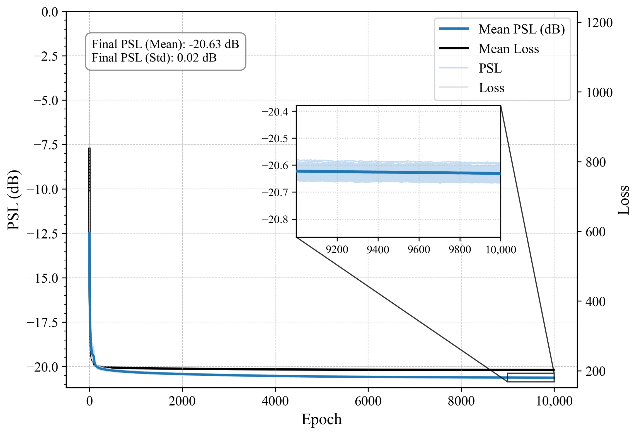
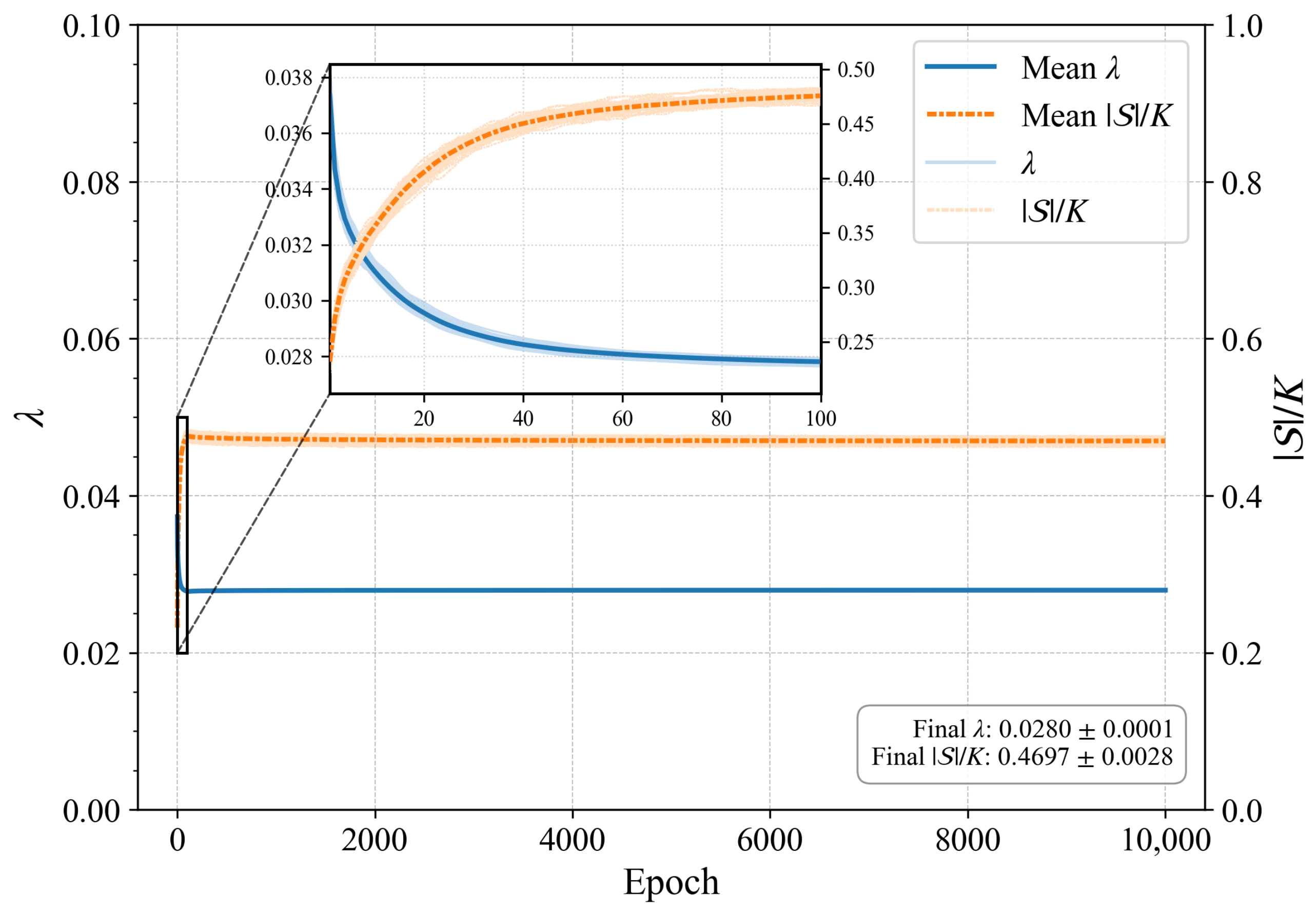
We adopted the typical configuration $M=10$, $N=128$, with uniformly distributed random initial phases, and performed 100 independent training runs to verify the convergence behavior and stability of the proposed method. Figure 4 shows the loss and PSL convergence curves from the 100 independent runs, while Figure 5 shows the evolution of the dynamic threshold $\lambda$ and the support fraction $\left|\mathcal{S}\right|/K$ (where $\left|\mathcal{S}\right|$ denotes the cardinality of the support set $\mathcal{S}$) during training. As Figure 4 shows, the PSL convergence exhibited two distinct stages. During the first 100 epochs, the PSL dropped rapidly from about $-12.5$ dB to about $-20$ dB; thereafter, it entered a slow fine-tuning phase, with the final mean stabilizing at $-20.63$ dB. The standard deviation across the 100 independent runs was only $0.021$ dB. The mean loss curve and the individual loss curves in Figure 4 are tightly concentrated and almost overlap, indicating that the proposed method shows little sensitivity to random initializations. The loss curves were smooth, reflecting the efficient convergence afforded by differentiability and the absence of training oscillations. Overall, the loss and PSL curves exhibited highly consistent trends; in the later stage the PSL continued to decrease even as the loss curve flattened, because by then many sidelobes already lay close to the peak, the peak sidelobe accounted for only a small fraction of the total weight, and its individual influence on the loss was correspondingly small.

Figure 5 reveals the evolution of the dynamic threshold and the sparsity of the support, which moved in opposite directions. During the first 100 epochs, the support fraction $\left|\mathcal{S}\right|/K$ stabilized at about $47\%$, and the dynamic threshold $\lambda$ completed its scale adjustment over the same period. After that, although the support size no longer changed significantly, the weight vector ${\mathit{\pi }}^{*}$ continued to be redistributed within the support, always assigning larger weights to those sidelobes with the highest current energy and driving the PSL toward the theoretical lower bound. Notably, the rapid descent during the first 100 epochs accounted for only a small fraction of the total training time but already realized about $90\%$ of the overall PSL improvement, owing to the differentiability of the proposed loss, which enabled accurate and rapid descent along the analytical gradient. Compared with the GD-based method, the proposed method reached a lower PSL because the loss function activated only about half of the sidelobes, suppressing the accumulated gradient contribution from low-energy sidelobes; in contrast, the LSE function assigns nonzero weights to all sidelobes, so all of them participate in the gradient and the accumulated noise constantly perturbs the gradient direction of the high-energy sidelobes.

5.3. Robustness to Initialization

To examine the effect of different initializations, we adopted the simulation setup of Section 5.1 (with $T_{max}={10}^4$ iterations) and replaced the random-phase initialization with five structured schemes, comparing the final PSL. We performed 20 independent runs per configuration and report the average PSL in

Table 1. Final PSL (dB) under different initialization schemes for four representative configurations. Each entry is the average over 20 independent runs.

Initialization	PSL (dB)
	$(\mathbf{4},\mathbf{64})$	$(\mathbf{4},\mathbf{256})$	$(\mathbf{4},\mathbf{1024})$	$(\mathbf{10},\mathbf{1024})$
Random phase	$-19.79$	$-25.79$	$-31.78$	$-29.63$
Zadoff–Chu sequence	$-19.79$	$-25.78$	$-31.77$	$-29.60$
Logistic chaotic map	$-19.78$	$-25.77$	$-31.78$	$-29.63$
8-bit quantized random	$-19.76$	$-25.79$	$-31.79$	$-29.61$
P4 polyphase code	$-19.40$	$-25.09$	$-30.05$	$-28.12$

.

The five schemes, spanning the random, quantized, chaotic, and polyphase-code families, are defined as follows: Random phase (the baseline of all preceding experiments) draws each chip phase independently from a uniform distribution, ${\phi }_u\left(n\right)\sim U(0,2\pi )$. Eight-bit quantized random phase draws each chip phase uniformly from 256 discrete levels, ${\phi }_u\left(n\right)=(2\pi /256)q_u\left(n\right)$ with $q_u\left(n\right)\sim \mathrm{Uniform}\{0,\dots ,255\}$. Logistic chaotic map generates each phase via the logistic recursion $x_u(n+1)=4x_u\left(n\right)\left(1-x_u\left(n\right)\right)$ with ${\phi }_u\left(n\right)=2\pi x_u\left(n\right)$, producing a deterministic yet aperiodic and ergodic sequence. Zadoff–Chu (ZC) sequence, a polyphase code with perfect periodic auto-correlation, is given for the code lengths considered (powers of two) by ${\phi }_u\left(n\right)=(\pi r_u/N)n^2$ with $gcd(r_u,N)=1$. P4 polyphase code generates the M waveforms from a common base code modulated by a waveform-dependent linear phase ramp, ${\phi }_u\left(n\right)=(\pi /N)n(n-N)+(2\pi u/M)n$, where $u=0,\dots ,M-1$, so that the waveforms differ only by a deterministic linear phase progression and are not mutually independent.

Two main observations can be drawn from Table 1. First, the random, 8-bit quantized, Logistic, and ZC initializations all converged to virtually the same PSL, with a maximum spread below $0.05$ dB for every configuration despite their markedly different structural origins. The algorithm is thus insensitive to the starting point as long as the initial waveforms are mutually uncorrelated; notably, the ZC sequence, despite its perfect auto-correlation, offers no measurable advantage over plain random phase. This confirms that the random-phase results reported earlier are not artifacts of a fortunate starting point and that the non-convex landscape does not trap the iterates in inferior minima. Second, the P4 initialization was the sole exception, converging to a PSL about $0.5$–$1.7$ dB higher. Because its M waveforms are merely linearly modulated copies of a single base code, the starting point lies in an almost flat region of the loss landscape with severely limited inter-waveform degrees of freedom; the descent therefore proceeded slowly and, within the fixed iteration budget, terminated at a higher PSL.

This behavior is explained by the limiting case of identical waveforms, $x_i\left(n\right)=x\left(n\right)$ for all i, in which every cross-correlation reduces to the common auto-correlation and the zero-delay cross-correlations attain the bound $r_{ij}\left(0\right)=N$. Substituting $x_i=x_u$ and $r_{ui}\left(0\right)=N$ into the analytical gradient in (35) leaves only the real-scalar zero-delay terms, so by the Wirtinger relation in (22), the phase gradient ${\nabla }_{{\mathit{\phi }}_u}\mathcal{L}$ vanishes identically. An all-identical initialization is thus a stationary point from which the algorithm cannot move, and the P4 case is a mild manifestation of the same mechanism: its waveforms are rigidly coupled rather than identical, so the gradient is small rather than exactly zero and convergence merely slows.

In summary, the proposed method does not require a specially designed starting point. Any initialization whose waveforms are mutually uncorrelated—random, quantized random, chaotic, or a decorrelated polyphase sequence—drives the PSL to essentially the same low value; only the degenerate case of highly correlated or identical waveforms, for which the phase gradient vanishes, needs to be avoided. Ensuring that the initial waveforms are mutually uncorrelated is therefore sufficient to guarantee convergence to a low PSL, confirming the robustness of the proposed method to initialization.

5.4. Doppler Tolerance Analysis

The proposed loss optimizes the zero-Doppler cut of the auto-/cross-ambiguity function, whereas Earth-observation MIMO-SAR systems operate under nonzero Doppler in practice. We therefore assessed the robustness of the optimized waveform set to an uncompensated Doppler shift. With the matched filters fixed at the zero-Doppler references $x_i\left(n\right)$ ($i=1,\dots ,M$), every echo $x_j\left(n\right)$ is modulated by a common Doppler ramp ${\mathrm{e}}^{\mathrm{j}2\pi \nu n}$, so that the Doppler-dependent cross-ambiguity function becomes

$$r_{ij}(\tau ,\nu )={\displaystyle \sum _{n=0}^{N-1}}{x}_i^{*}\left(n\right)x_j(n+\tau ){\mathrm{e}}^{\mathrm{j}2\pi \nu n},\nu =f_d{T}_c,$$

(55)

where $\tau$ is the delay lag, $\nu$ is the normalized Doppler frequency per chip, $f_d$ is the Doppler frequency, $T_c$ is the chip duration, N is the code length, and $T=N{T}_c$ is the total pulse duration. The normalized phase walk accumulated over the whole pulse is $\nu N=f_{d}T$. All sidelobe magnitudes are normalized by the zero-Doppler matched-filter peak N, so that the curves are referenced to the ideal zero-Doppler gain. Since the chip-rate bandwidth $B_s$ (tens to hundreds of MHz) greatly exceeds the intra-pulse Doppler frequency $f_d$ (at most a few kHz), we have $\nu =f_d/B_s\ll 1$, and $\nu N$ amounts to only a small fraction of a cycle in practice, typically satisfying $\nu N\ll 0.1$. We therefore swept $\nu N\in [0,0.5]$, which already covers far beyond the operational range.

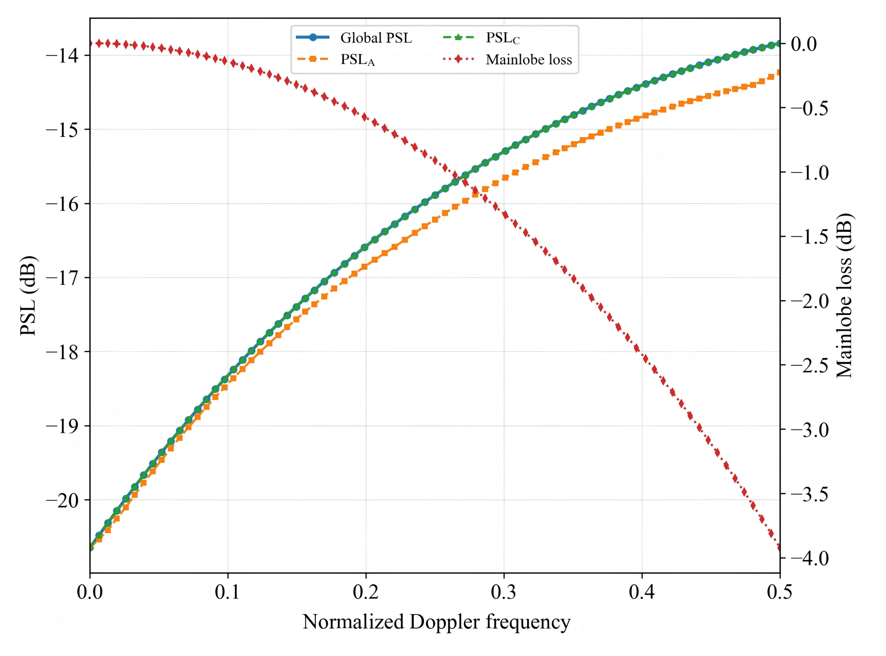
As shown in Figure 6, at $\nu N=0$, the global PSL equaled $-20.63$ dB, coinciding with the value obtained in Section 5.2 and thereby cross-validating the evaluation; the global PSL curve overlapped the cross-correlation PSL throughout the entire sweep range, indicating that for $M=10$, the worst sidelobe is governed by the cross-correlation terms, as expected from the large number of cross pairs. Furthermore, the PSL degraded smoothly and monotonically with Doppler, without any abrupt collapse: within the operationally relevant range $\nu N\le 0.1$, the global PSL rose by only about $2.30$ dB (to $-18.33$ dB), while the mainlobe loss stayed below $0.16$ dB, so the orthogonality of the set was essentially preserved; even at the extreme $\nu N=0.5$, the global PSL remained at $-13.81$ dB. In summary, the optimized waveform set exhibits good robustness to uncompensated Doppler over the practically relevant operating range.

5.5. Robustness to Phase Quantization

The signal model in Section 2 assumes a continuous phase ${\phi }_u\left(n\right)\in [0,2\pi )$, whereas a practical MIMO-SAR transmitter realizes the phase through a digital phase shifter with finite resolution. We denote the quantization bit-width by b. A b-bit phase shifter provides $Q=2^b$ uniformly spaced phase states with spacing ${\Delta }_{\phi }=2\pi /2^b$. Rounding each optimized phase to the nearest available state gives

$${\tilde{\phi }}_u\left(n\right)={\displaystyle \frac{2\pi }{2^b}}⌊{\displaystyle \frac{2^b}{2\pi }}{\phi }_u\left(n\right)+{\displaystyle \frac{1}{2}}⌋,$$

(56)

where $\lfloor ·\rfloor$ is the floor operator and ${\tilde{\phi }}_u\left(n\right)$ is the quantized phase; the resulting rounding error is confined to $[-{\Delta }_{\phi }/2,{\Delta }_{\phi }/2]$.

To assess the practical impact of this quantization on waveform performance, we applied Equation (56) to the continuous-phase optimum obtained in Section 5.3 and re-evaluated the PSL for $b\in \{4,5,6,7,8\}$ under four representative configurations $(M,N)$. The results are summarized in

Table 2. Normalized PSL of the optimized waveforms after b-bit phase quantization for four representative configurations $(M,N)$. $Q=2^b$ is the number of available phase states, and $\Delta$PSL is the increase in PSL relative to the continuous case (a positive value indicates degradation). “—” indicates not applicable (continuous-phase baseline).

b	Q	$(4,64)$		$(4,256)$		$(4,1024)$		$(10,1024)$
		PSL	$\Delta$ PSL	PSL	$\Delta$ PSL	PSL	$\Delta$ PSL	PSL	$\Delta$ PSL
Continuous	∞	$-19.79$	—	$-25.79$	—	$-31.78$	—	$-29.63$	—
4	16	$-17.53$	$+2.26$	$-22.79$	$+3.00$	$-28.86$	$+2.92$	$-26.76$	$+2.87$
5	32	$-18.45$	$+1.34$	$-24.21$	$+1.58$	$-30.24$	$+1.54$	$-28.19$	$+1.44$
6	64	$-18.99$	$+0.80$	$-25.04$	$+0.75$	$-30.98$	$+0.80$	$-28.93$	$+0.70$
7	128	$-19.37$	$+0.42$	$-25.44$	$+0.35$	$-31.33$	$+0.45$	$-29.34$	$+0.29$
8	256	$-19.59$	$+0.20$	$-25.65$	$+0.14$	$-31.59$	$+0.19$	$-29.48$	$+0.16$

, where $\Delta \mathrm{PSL}$ denotes the increase in PSL relative to the continuous-phase baseline.

As shown in Table 2, the PSL degraded monotonically as the quantization resolution b decreased, but the degradation was bounded and controllable: at the coarsest resolution $b=4$, the loss was about $2.3$–$3.0$ dB; increasing b to 6 already reduced the degradation to about $0.7$–$0.8$ dB; and at $b=8$, the degradation dropped further to about $0.1$–$0.2$ dB, essentially matching the continuous-phase result. This trend was consistent across all four $(M,N)$ configurations and shrank smoothly as b increased. Overall, a commercially common 6-bit phase shifter is sufficient to achieve satisfactory performance, while moving to 8-bit resolution further limits the degradation to within $0.2$ dB, yielding an even lower PSL; these results confirm that the proposed continuous-phase design can be directly deployed on practical quantized hardware, with the required resolution selected according to the desired performance–cost trade-off.

5.6. Comparison with Other Methods

5.6.1. Adaptability Across Code Lengths

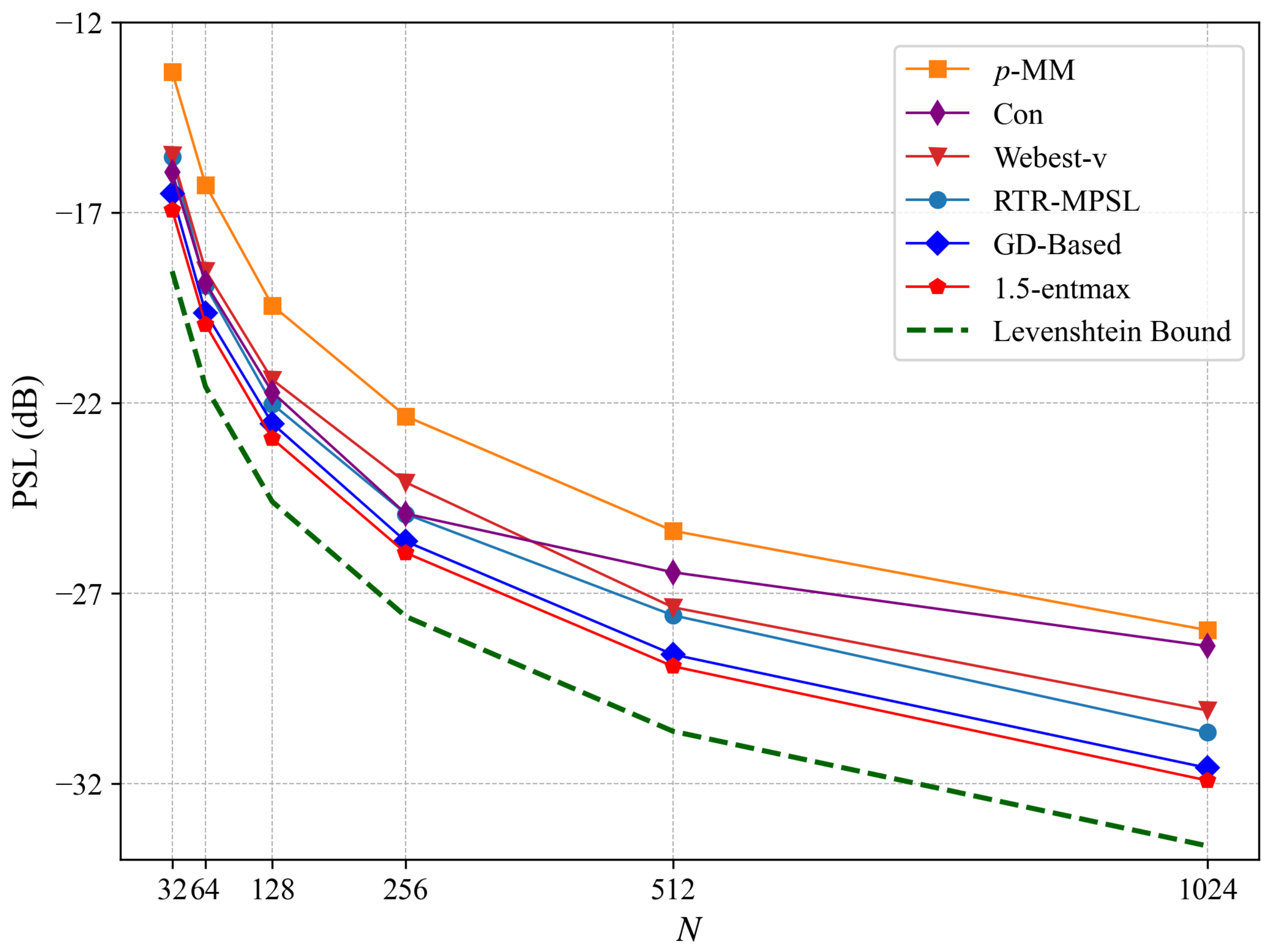
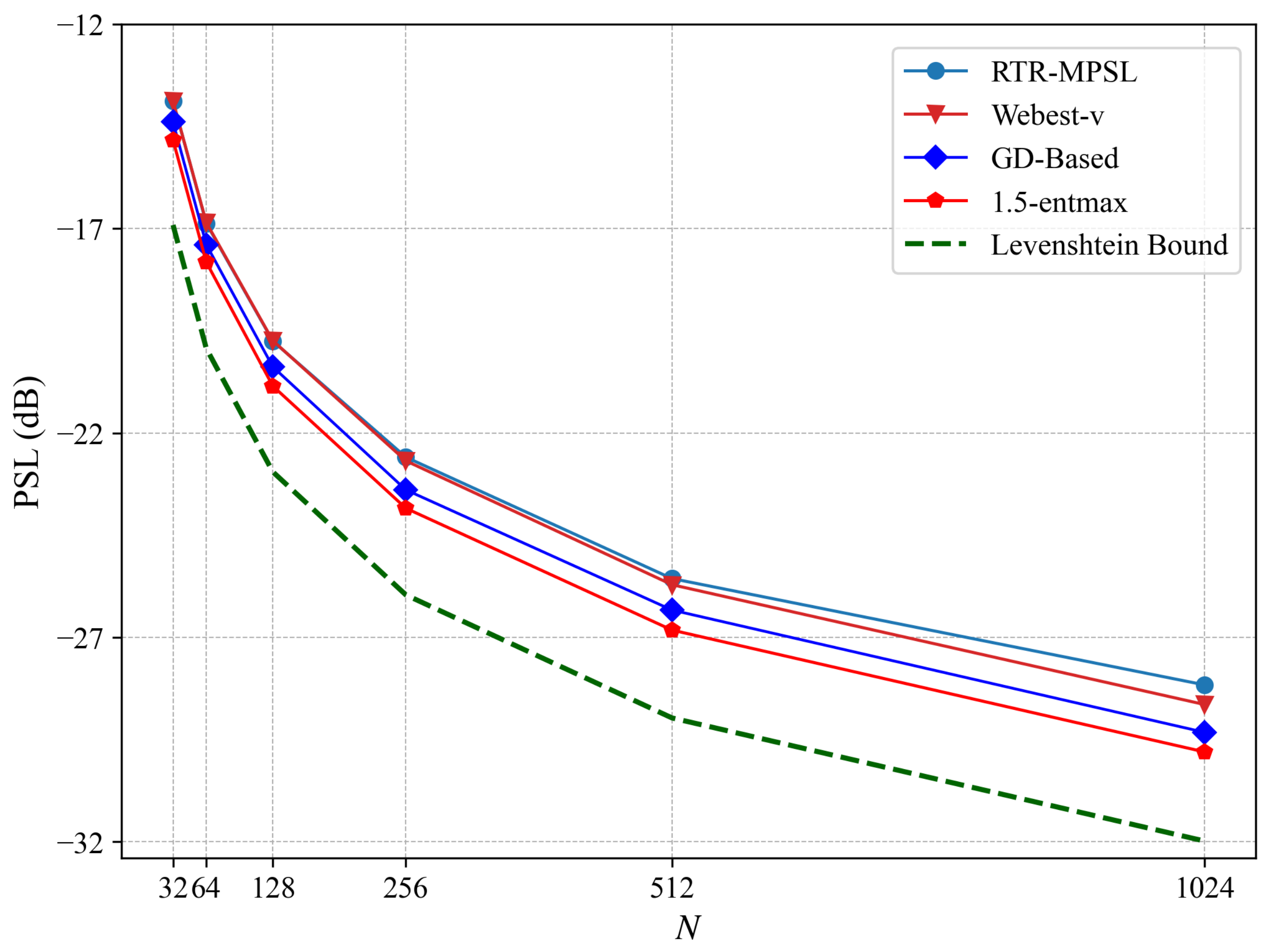
With $M=4$ fixed and $N\in \{32,64,128,256,512,1024\}$, we systematically evaluated the PSL performance of each method. The results are shown in Figure 7.

The PSL of all methods decreased monotonically with N, in agreement with the trend of the Levenshtein bound. The proposed method achieved the lowest PSL at every code length. For $N=1024$, for example, the PSL of 1.5-entmax reached $-31.79$ dB, which was $1.12$ dB lower than RTR-MPSL, $1.70$ dB lower than WeBEST-v, $3.39$ dB lower than Con, and $3.91$ dB lower than p-MM. It was only $1.86$ dB above the Levenshtein bound, making it the closest result to the theoretical limit in this comparison.

The performance of Con degraded noticeably for $N\ge 512$, primarily because its fixed weight ratio cannot adapt to the sidelobe distribution as it changes with N, and because the number of parameters in the residual network grows rapidly with M and N so that a fixed network architecture cannot readily accommodate larger waveform dimensions. p-MM was the weakest at every code length, mainly because the numerical instability introduced by the large p-value continues to worsen as the total number of sidelobes grows [29]. The advantage of 1.5-entmax over GD-based grew monotonically with N, primarily because the total number of sidelobes increases at the rate of $\mathcal{O}\left(M^{2}N\right)$, so the gradient noise accumulated by LSE becomes more pronounced, while the strict-truncation mechanism of 1.5-entmax prevents this from accumulating with scale.

5.6.2. Adaptability Across Numbers of Waveforms

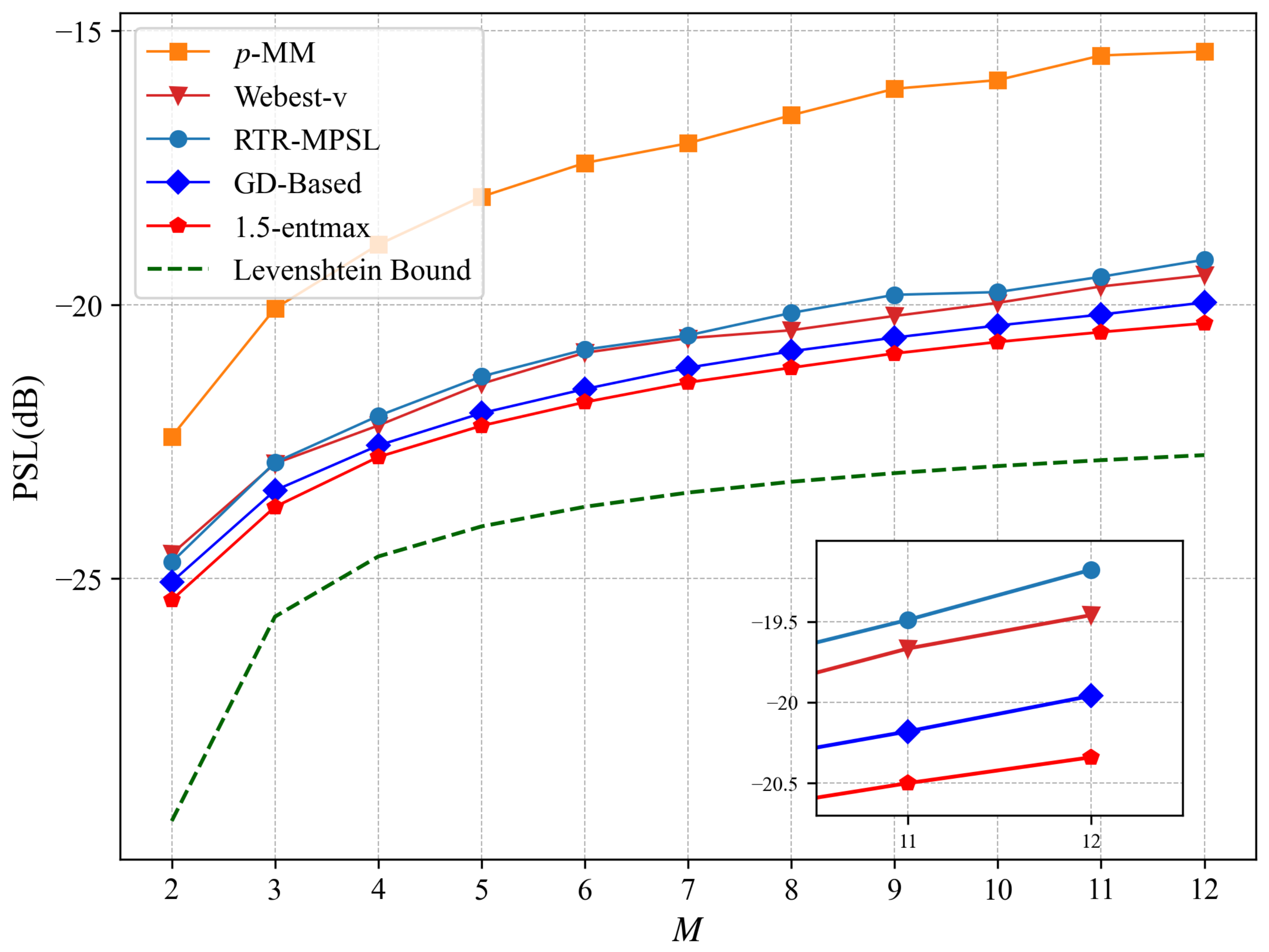
To compare adaptability with respect to the number of waveforms, we fixed $N=128$, and let $M\in \{2,3,\dots ,12\}$. The performance of each method under different numbers of waveforms is shown in Figure 8.

The PSL of all methods increased monotonically with M, again in agreement with the trend of the Levenshtein bound: the number of cross-correlation components grows at rate $(M^{2}N-M)$, and the optimization becomes correspondingly more difficult. Further, 1.5-entmax achieved the lowest PSL for every value of M from 2 to 12, and its margin over GD-based grew monotonically with M (from $0.10$ dB at $M=2$ to $0.33$ dB at $M=12$). This trend corroborates the analysis with respect to N in Section 5.6: regardless of whether the total number of sidelobes increases through larger N or larger M, the cumulative effect of LSE gradient noise is amplified, and the sparse-truncation advantage of 1.5-entmax grows accordingly.

The 1.5-entmax curve was smooth across the entire range of M, while WeBEST-v and RTR-MPSL displayed local fluctuations that reflected their sensitivity to initialization and step size. The gap between p-MM and 1.5-entmax widened from about 3 dB at $M=2$ to about 5 dB at $M=12$, indicating that the numerical instability introduced by the large p-value worsened further in high-dimensional cross-correlation scenarios.

5.7. Computational Complexity and Scalability

Table 3. Computational complexity of the compared methods.

Method	Per-Iteration Computational Complexity	Execution Platform	Loss-Function Hyperparameters
1.5-entmax	$\mathcal{O}(M^{2}NlogN)$	GPU/CPU	None
GD-based [35]	$\mathcal{O}(M^{2}NlogN)$	GPU	Smoothing parameter t
Con [28]	$\mathcal{O}(M^{2}NlogN+L·N_{\mathrm{net}})$	GPU	Five weighting coefficients $({\omega }_1,\dots ,{\omega }_5)$
p-MM [29]	$\mathcal{O}(M^{2}NlogN)$	CPU	Order p
RTR-MPSL [31]	$\mathcal{O}\left(max\{M^2{N}^2,M^{2}N{log}_2(p/2)\}\right)$	CPU	Order p
WeBEST-v [25]	$\mathcal{O}(n_{\mathrm{bt}}·M^{2}NlogN)$	CPU	Order p

Note: L is the number of layers in the Con network, $N_{\mathrm{net}}$ is the number of operations in a single forward pass, and $n_{\mathrm{bt}}$ is the average number of backtracking line-search steps per iteration in WeBEST-v. For RTR-MPSL with $p=8$, ${log}_2(p/2)=2\ll N^2$, so the per-iteration cost is dominated by $\mathcal{O}\left(M^2{N}^2\right)$. The proposed method is highlighted in bold.

summarizes the per-iteration computational complexity, execution platform, and loss-function hyperparameters of the compared methods, and

Table 4. Time required by each method to reach the target PSL. “—” indicates that the target was not reached within 2 h.

$(\mathit{M},\mathit{N})$	Target PSL (dB)	Time (s)
		1.5-Entmax (GPU)	1.5-Entmax (CPU)	GD-Based	RTR-MPSL	WeBEST-v	Con	p-MM
$(4,64)$	$-18$	0.53	0.11	7.97	0.24	2.14	1.22	3.45
$(4,256)$	$-24$	0.53	0.19	9.54	3.27	7.84	16.33	163.88
$(4,1024)$	$-30$	0.56	0.88	5.15	55.61	14.79	—	—
$(10,1024)$	$-28$	0.69	1.01	12.83	311.45	92.49	—	—
$(128,1024)$	$-25$	9.83	140.62	1700.33	—	—	—	—

Note: Bold values indicate the results of the proposed method (GPU and CPU implementations), which attains the shortest time to the target PSL in each configuration.

reports the time each method requires to reach the target PSL. The proposed method, GD-based, and p-MM share the same theoretical complexity of $\mathcal{O}(M^{2}NlogN)$, yet the proposed method is far faster in practice—even on the same CPU platform. On equal footing with the CPU baselines, the CPU version of 1.5-entmax reaches every target PSL in at most $1.01$ s for $(M,N)$ up to $(10,1024)$ and in $140.62$ s at $(128,1024)$; by contrast, RTR-MPSL and WeBEST-v already require $311.45$ s and $92.49$ s respectively at $(10,1024)$ and fail to converge within two hours at $(128,1024)$, while p-MM exceeds the budget from $(4,1024)$ onward. Two factors explain this gap. First, only the in-support sidelobes participate in the effective gradient at each iteration, so the actual cost is well below that of the dense GD-based gradient. Second, the sparse, noise-free gradient lets each iteration focus on the high-energy-sidelobe subset, sharply reducing the iteration count: at $(128,1024)$, the proposed method converges within about 100 epochs, whereas GD-based needs more than 3000 epochs.

The per-iteration cost of RTR-MPSL is dominated by the $\mathcal{O}\left(M^2{N}^2\right)$ term under our simulation parameters: at $N=1024$ and $M=10$, it reaches the order of ${10}^8$, so the method does not converge within two hours on the CPU. p-MM has the same $\mathcal{O}(M^{2}NlogN)$ order as the proposed method but runs on the CPU and requires a very large number of iterations, with the numerical instability of large p further hindering convergence as N or M grows. The complexity of WeBEST-v carries the backtracking-step factor $n_{\mathrm{bt}}$, and under the combined pressure of sequential CPU execution and a huge number of sidelobes, its runtime already reached 92 s at $N=1024$, $M=10$, becoming infeasible at larger scales.

We next consider medium-to-large-scale configurations by increasing M from 4 to 10 while varying $N\in \{32,64,128,256,512,1024\}$. The total number of sidelobes grows by a factor of about three relative to the $M=4$ case. At this scale, both p-MM and Con failed to reach an acceptable PSL target within 2 h when $N\ge 512$. Figure 9 compares the remaining methods: GD-based, RTR-MPSL, WeBEST-v, and 1.5-entmax.

It can be seen that 1.5-entmax outperformed the other methods at every code length. For $N=1024$, for instance, 1.5-entmax reached $-29.63$ dB, which was $0.26$ dB lower than GD-based ($-29.32$ dB) and $1.42$ dB lower than RTR-MPSL ($-28.16$ dB) and was $2.40$ dB above the Levenshtein bound. Comparing these results with those for $M=4$, $N=1024$ in Section 5.6, we see that the advantage of 1.5-entmax over GD-based grew with M, again confirming the structural advantage of the sparse-truncation mechanism in scenarios with a rapidly increasing number of sidelobes.

5.8. Adaptability Under Ultra-Large-Scale Configurations

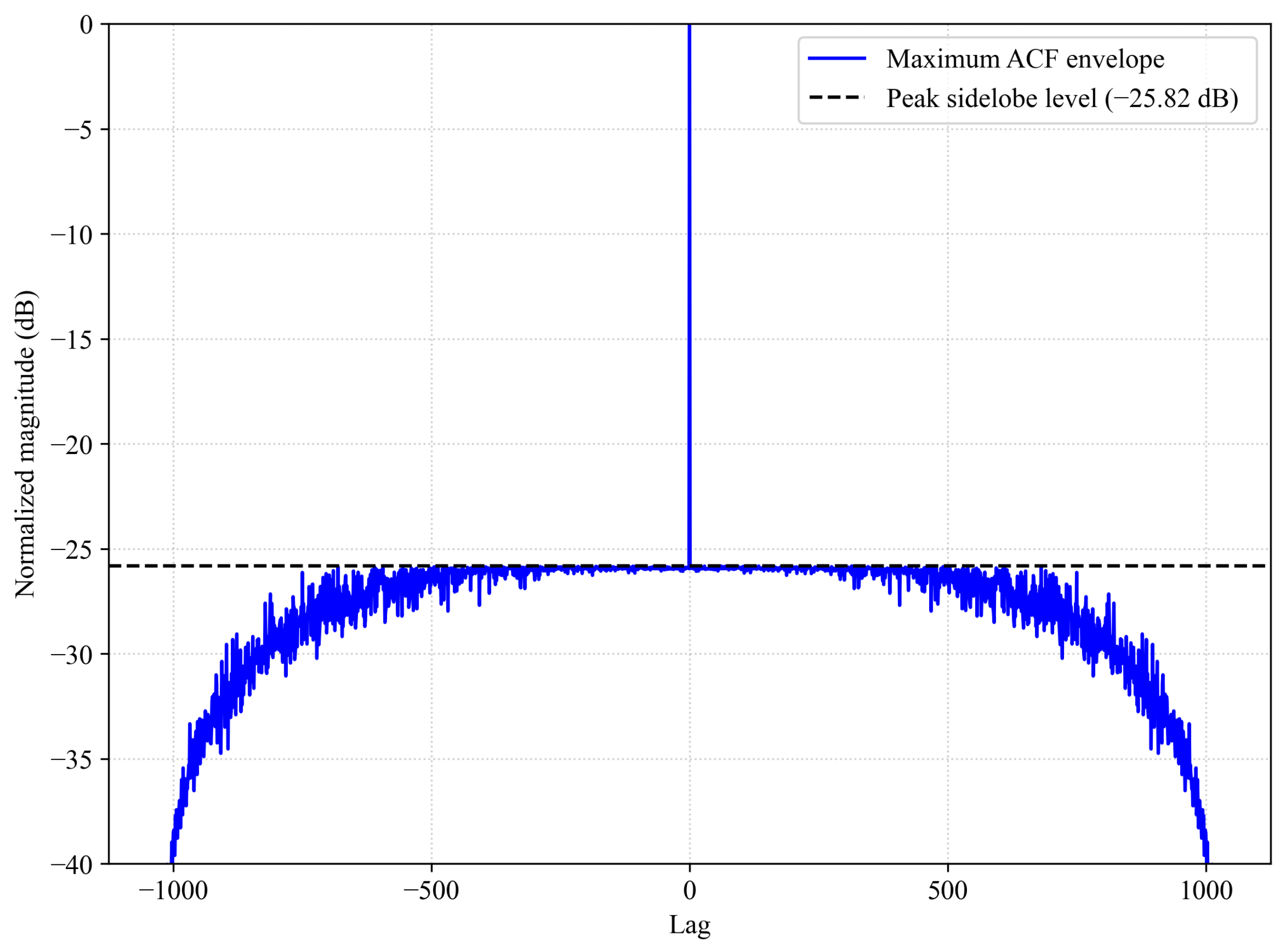
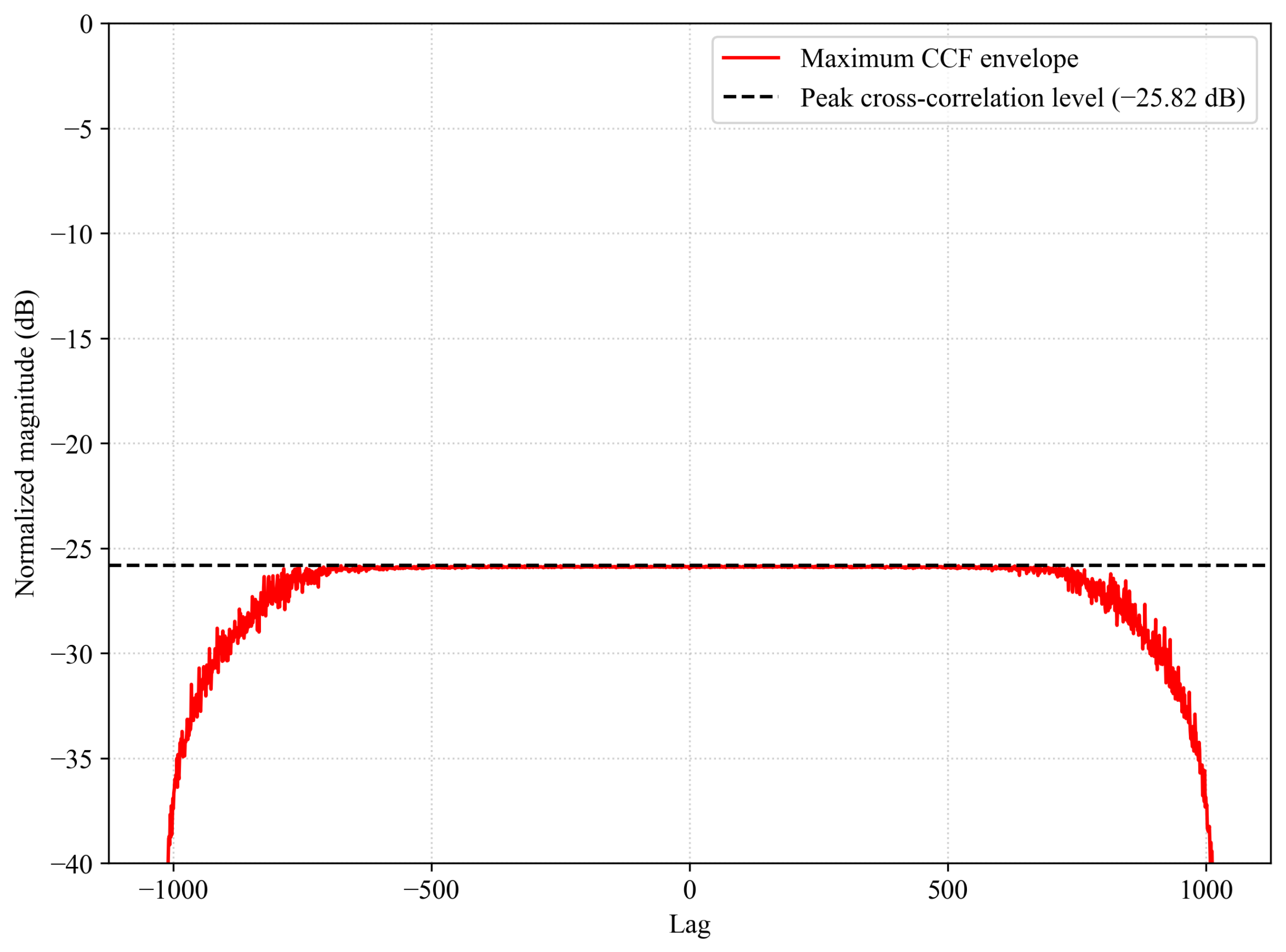
Figure 10 and Figure 11 show the auto-correlation and cross-correlation envelopes (in dB) of the waveforms designed under the ultra-large-scale configuration $(M,N)=(128,1024)$.

Each envelope is defined as the maximum magnitude across waveform pairs at each delay:

$${\rho }_a\left(\tau \right)=\underset{m}{max}{\displaystyle \frac{|r_{mm}\left(\tau \right)|}{N}},{\rho }_c\left(\tau \right)=\underset{m\ne l}{max}{\displaystyle \frac{|r_{ml}\left(\tau \right)|}{N}}.$$

(57)

All sidelobes were suppressed below $-25$ dB, and the envelopes were highly uniform. Under the ultra-large-scale configuration $(M,N)=(128,1024)$, the total number of sidelobes K exceeds $3.4\times {10}^7$. At this scale, the per-iteration cost of RTR-MPSL is $M^2{N}^2\approx 1.72\times {10}^{10}$, so the method does not converge within 2 h on the CPU. WeBEST-v is likewise infeasible, owing to its CPU-sequential backtracking line search. p-MM fails because of the large number of iterations required on the CPU, compounded by the numerical instability introduced by large p. GD-based did complete the optimization on the GPU but took about 1700 s. On the same GPU, the proposed 1.5-entmax method reached the $-25$ dB target in only $9.83$ s—a $173\times$ speedup over GD-based. The CPU version of the proposed method reached the same target in $140.62$ s, so that even without GPU parallelism, it was about $12\times$ faster than the GPU-based GD-based baseline, with the GPU providing a further $14.3\times$ reduction.

The proposed method handles such large-scale problems efficiently for three main reasons: (i) the 1.5-entmax transform is both sparse and differentiable, ensuring fast and accurate gradient descent at a per-iteration complexity of only $\mathcal{O}(M^{2}NlogN)$; (ii) the entire loss computation consists of regular tensor operations that map naturally onto GPU parallelism; and (iii) the analytical Jacobian bypasses the inner Newton iteration, so the memory footprint of the computation graph does not grow with the number of Newton steps. These results demonstrate the engineering viability of the proposed method for next-generation large-scale MIMO-SAR systems.

5.9. Ablation Study

To quantify the contribution of each design component, we conducted a component-wise ablation study targeting four core elements: (1) the 1.5-entmax sparse weighting transform; (2) the normalization preprocessing; (3) the analytical Jacobian operator; and (4) GPU-parallel acceleration. In each ablation variant, a single component was removed or replaced while all other settings remained identical to the complete method. Experiments were performed on the same five waveform sizes $(M,N)$ as in Section 5, each trained for ${10}^4$ iterations. Two metrics were recorded: the final PSL (after ${10}^4$ iterations) and the time to target $T_{\mathrm{tgt}}$ (the time required to reach the target PSL; “—” indicates that the target was not reached within ${10}^4$ iterations). The target PSL for each configuration followed the values used in Table 4.

The four ablation variants are defined as follows:

• Without 1.5-entmax. The 1.5-entmax transform is replaced by the softmax ($\alpha =1$) from the same family; the weighted-loss structure is otherwise unchanged.
• Without normalization. The normalization of sidelobe magnitudes by the theoretical upper bound N is removed; raw magnitudes $\in [0,N]$ are fed directly into the transform, isolating the effect of normalization on the adaptive threshold $\lambda$.
• Without analytical Jacobian. The complete loss and normalization are retained, but the back-propagation through the entmax step uses automatic differentiation of the Newton iteration that solves for $\lambda$ instead of the analytical Jacobian.
• Without GPU acceleration. The CPU implementation of the proposed method introduced in Section 5.1 is used here, executing the identical algorithm in MATLAB without GPU parallelism. Because the analytical gradient is evaluated from the same closed-form expression in both versions, their difference in runtime reflects the GPU parallelism rather than any change in the optimization itself.

Table 5. Ablation results.

Ablation Setting	Final PSL (dB)					Time to Target ${\mathit{T}}_{\mathbf{tgt}}$ (s)
	$(\mathbf{4},\mathbf{64})$	$(\mathbf{4},\mathbf{256})$	$(\mathbf{4},\mathbf{1024})$	$(\mathbf{10},\mathbf{1024})$	$(\mathbf{128},\mathbf{1024})$	$(\mathbf{4},\mathbf{64})$	$(\mathbf{4},\mathbf{256})$	$(\mathbf{4},\mathbf{1024})$	$(\mathbf{10},\mathbf{1024})$	$(\mathbf{128},\mathbf{1024})$
Complete method	$-\mathbf{19}.\mathbf{79}$	$-\mathbf{25}.\mathbf{79}$	$-\mathbf{31}.\mathbf{78}$	$-\mathbf{29}.\mathbf{63}$	$-\mathbf{25}.\mathbf{82}$	0.53	0.53	0.56	0.69	9.83
Quality-related components
Without 1.5-entmax	$-19.15$	$-24.89$	$-30.55$	$-28.38$	$-23.78$	2.20	2.95	6.11	1.45	—
Without normalization	$-19.26$	$-24.54$	$-30.16$	$-28.10$	$-22.85$	0.42	1.36	40.03	49.47	—
Speed-related components
Without analytical Jacobian	$-19.78$	$-25.79$	$-31.78$	$-29.61$	$-25.81$	0.67	0.67	0.82	0.89	12.82
Without GPU acceleration	$-19.79$	$-25.77$	$-31.77$	$-29.62$	$-25.82$	0.11	0.19	0.88	1.01	140.62

Note: Bold indicates the complete (proposed) method and its results.

reports the results.

Contribution of 1.5-entmax to suppression quality. Replacing the 1.5-entmax transform with softmax increased the final PSL across all configurations: by $0.64$ dB for $(4,64)$, $0.90$ dB for $(4,256)$, $1.23$ dB for $(4,1024)$, $1.25$ dB for $(10,1024)$, and $2.04$ dB for $(128,1024)$, where the target could not be reached within ${10}^4$ iterations. The degradation grew monotonically with the total number of sidelobes K, consistent with the analysis in Section 3; as K increases, the gradient noise accumulated by the non-sparse softmax weighting becomes more pronounced, whereas the strict truncation of 1.5-entmax prevents this accumulation.

Contribution of normalization. Removing normalization degraded both the final PSL and convergence speed. The PSL worsened by $0.53$–$2.97$ dB, with the degradation intensifying as N grew. More notably, the time to target increased sharply: at $N=1024$, it rose from below 1 s to $40.03$ s for $(4,1024)$ and $49.47$ s for $(10,1024)$, and for $(128,1024)$, the target could not be reached. Without normalization, the transform operates on raw magnitudes spanning $[0,N]$; a larger N perturbs the dynamic threshold $\lambda$ more strongly, moving it away from its ideal value. Normalizing by N makes the threshold depend only on the relative sizes of the sidelobes, confirming the necessity of this preprocessing step.

Contribution of the analytical Jacobian operator. Replacing the analytical Jacobian with automatic differentiation of the Newton iteration yielded a nearly identical final PSL, verifying the mathematical equivalence of the two approaches. As an independent check on the correctness of the analytical gradient itself, we compared Equation (39) against a central finite-difference reference and against automatic differentiation on small random instances ($M\le 4$, $N\le 32$). The maximum relative error was below ${10}^{-6}$, confirming that the closed-form gradient is implemented correctly; the “without analytical Jacobian”variant below then isolates its computational benefit at equal accuracy. The difference lies in computational overhead. On larger-scale configurations, the automatic-differentiation variant took about $1.3$–$1.5\times$ longer than the complete method, confirming that the analytical Jacobian improves computational efficiency by avoiding the expansion of the computation graph over the Newton steps.

Contribution of GPU acceleration. Running the same algorithm on the CPU produced a nearly identical PSL, with the benefit of GPU acceleration emerging as the problem scale increased. On small-scale configurations, the CPU implementation was faster because of the overhead of transferring data from the CPU to the GPU in the GPU version; as $(M,N)$ grew, the parallelism of the GPU gradually dominated. At $(128,1024)$, the GPU reduced the time to target from $140.62$ s to $9.83$ s, which validates the acceleration advantage of the proposed framework for large-scale real-time MIMO-SAR waveform design.

6. Discussion

The experiments point to a single underlying reason for the consistent advantage of the proposed loss. The PSL is the maximum over $K=\mathcal{O}\left(M^{2}N\right)$ sidelobes, yet it is governed by only the few highest-energy ones, so its active set is a vanishingly small fraction of all sidelobes. Smooth surrogates such as LSE spread gradient mass over the entire set, diluting the signal of the decisive sidelobes by a factor that grows with K. This is why the margin over the GD-based baseline widens monotonically with both N and M (Figure 7, Figure 8 and Figure 9) and why the softmax ablation degrades in proportion to K: the dilution, and not any incidental numerical effect, is the mechanism. By truncating the support, 1.5-entmax aligns the gradient’s support with the objective’s active set—the natural matching between optimizer and objective for a max-type criterion.

Normalization is the second indispensable ingredient. Without it, the scale sensitivity of 1.5-entmax couples the dynamic threshold $\lambda$ to the absolute sidelobe magnitude, which itself varies with N; the ablation shows that this coupling not only raises the final PSL but, more severely, slows convergence by one to two orders of magnitude at large N. Normalizing by the Cauchy–Schwarz upper bound N confines all inputs to $[0,1]$ and makes $\lambda$ depend only on the relative sidelobe distribution, which is what allows a single, untuned loss to operate across waveform sizes differing by orders of magnitude.

Several limitations remain. First, $\alpha =1.5$ is motivated by differentiability and the avoidance of fractional root extractions rather than by a proof of optimality, and the optimal $\alpha$ within $(1,2)$ remains open. Second, the present formulation addresses only constant-modulus phase-coded waveforms under the single PSL metric, without practical constraints such as spectral shaping or the joint design of transmit waveforms and mismatched receive filters. These limitations delineate the scope of the reported gains and motivate the extensions below.

7. Conclusions

This paper addressed the non-differentiability and gradient-noise problems of direct PSL minimization in MIMO-SAR orthogonal waveform design. We proposed a loss function built on the 1.5-entmax sparse transform that is simultaneously differentiable and sparse: it concentrates the gradient on the high-energy sidelobes that determine the PSL while strictly truncating the low-energy ones to remove their gradient noise. A normalization step based on the Cauchy–Schwarz upper bound eliminates the transform’s scale sensitivity and makes its dynamic threshold adapt automatically across waveform sizes, so that no loss-function hyperparameter requires tuning. We derived a closed-form analytical gradient and, through a custom analytical Jacobian operator, embedded the loss into a GPU-accelerated deep learning framework that treats the waveform phases as the only learnable parameters and keeps the per-iteration complexity at $\mathcal{O}(M^{2}NlogN)$.

Extensive simulations showed that the method attains the lowest PSL across all evaluated waveform sizes, consistently approaching the Levenshtein bound, and remains robust to initialization, uncompensated Doppler, and phase quantization. In ultra-large-scale settings ($M=128$, $N=1024$), it reached the target PSL roughly two orders of magnitude faster than the existing state-of-the-art method on the same GPU and about an order of magnitude faster even in its CPU implementation, confirming that the gain is algorithmic rather than a mere consequence of hardware. These properties establish the method’s viability for real-time, online waveform synthesis in next-generation MIMO-SAR systems.

Future work will pursue a theoretical characterization of the optimal $\alpha$ within $(1,2)$ and extend the framework to spectrally constrained waveforms, joint waveform–mismatched-filter design, and validation on real MIMO-SAR hardware.