Seismic Inversion Based on Mamba and ResUNet++

Highlights

What are the main findings?

• We developed DMamUNet, a seismic inversion framework that fuses Mamba modules with ResUNet++ and deformable convolution. We validated the framework across diverse scenarios, including the Marmousi model, post-stack impedance inversion, and pre-stack multi-parameter inversion, demonstrating superior vertical resolution and lateral continuity.
• The composite loss function combining a multitrace-to-multitrace (M2M) supervision strategy further improves feature learning and generalization. A pre-training and fine-tuning transfer learning approach is employed to address the challenge of limited well-log data, which improves inversion robustness.

What are the implications of the main findings?

• DMamUNet integrates Mamba’s long-range dependency modeling with the multi-scale, adaptive local feature extraction of ResUNet++ and deformable convolution. This hybrid architecture effectively captures both global parameter trends in seismic data and complex, nonstationary local geological features.
• DMamUNet outperforms the current approaches, including TransUNet and FCRN, in terms of inversion precision and structural continuity, offering a tool for high-precision geophysical exploration and reservoir characterization.

Abstract

Seismic inversion is crucial for reservoir characterization. Conventional inversion methods are frequently limited by low resolution and the requirement for low-frequency models. Although deep learning has shown promising performance in seismic parameter inversion, convolution-based networks mainly rely on local receptive fields and cannot explicitly capture the long-range dependencies along seismic traces, which limits their ability to recover the overall subsurface parameter trends. To alleviate this problem, we propose a Mamba-based seismic inversion network, termed DMamUNet. Built on the ResUNet++ backbone, DMamUNet introduces Mamba modules into the encoder–decoder framework to model long-sequence contextual information and global parameter variation trends, while deformable convolution blocks are used to enhance the adaptive representation of local nonstationary features. In addition, a multitrace-to-multitrace (M2M) supervision strategy and a composite loss combining well-log parameter supervision with seismic reconstruction are adopted to further improve feature learning and generalization. Experiments on the Marmousi model, post-stack field data, and pre-stack field data demonstrate that DMamUNet outperforms conventional methods. Specifically, DMamUNet significantly enhances both inversion accuracy and lateral continuity. In the post-stack field data experiment, the proposed DMamUNet achieves a 78.22% reduction in blind well mean squared error (MSE) compared with FCRN, and a 14% MSE reduction relative to TransUNet. Additionally, DMamUNet predictions on pre-stack field data exhibit higher resolution and better spatial continuity, highlighting its superiority for improving reservoir characterization.

1. Introduction

In the context of hydrocarbon reservoir characterization and coalfield shale distribution prediction, seismic inversion remains a primary methodology for bridging the gap between seismic data and subsurface properties [1,2]. Its objective is to estimate seismic parameters via seismic data constrained by well-log information or physical laws. Traditional inversion techniques, however, frequently struggle with limited resolution, non-uniqueness, and strong dependence on low-frequency models, which restrict the robustness under complex geological conditions [3,4]. These limitations motivate the development of data-driven inversion methods capable of capturing complex nonlinear seismic-geological mappings.

With the emergence of deep learning (DL) technologies, data-driven approaches have provided new possibilities for seismic inversion through powerful nonlinear mapping capabilities [3]. A review by Song et al. [5] summarized the rapid progress of deep learning in seismic inversion, demonstrating its feasibility and potential. Among various deep learning models, Convolutional Neural Network (CNN) -based models represented by U-Net are the most widely used and have achieved promising results. However, convolution operations act as local filters that effectively capture seismic reflection textures but often fail to model long-range dependencies essential for low-frequency impedance trend recovery [4]. In fact, a seismic trace is a long temporal sequence, and its seismic parameter responses depend not only on local reflection details but also on broader contextual information [6]. In essence, seismic data exhibit correlations in both temporal and spatial dimensions. Along the temporal dimension, the associated elastic parameters contain not only local variation patterns but also global trends, which reflect the overall vertical background shaped by large-scale sedimentary processes. Therefore, effectively capturing the global information embedded in seismic traces is particularly important for improving inversion performance. Although CNN-based methods attempt to enlarge the receptive field by using larger convolution kernels or stacking more convolutional layers, both strategies have practical limitations. Excessively enlarging convolution kernels increases computational cost and may reduce the effectiveness of feature extraction, while overly deep network architectures may lead to progressive information loss during training. As a result, by leveraging the temporal dependency-capturing capabilities of recurrent structures, such as recurrent neural networks (RNNs) [7], as well as advanced iterations like long short-term memory (LSTM) [8] and gated recurrent unit (GRU) [9], various models have been applied to seismic sequence modeling. For example, Guo et al. [8] utilized bidirectional LSTM networks to achieve impedance inversion without wavelet estimation, obtaining results with good lateral continuity. Wang et al. [9] achieved accurate S-wave velocity prediction through a fusion network combining convolution and GRU. Although these models improve temporal dependency modeling to some extent, their sequential iterative processing modes often lead to limited parallelization, making it difficult to efficiently process long seismic sequences [10].

Transformers provide an effective solution for long-range dependency modeling through self-attention mechanism [11], and CNN-Transformer hybrid models have shown improved performance in seismic inversion [6,12]. However, the quadratic computational complexity of the self-attention mechanism leads to substantial computational cost, which limits its efficiency for long seismic traces and large-scale seismic sections. Recently, Mamba, as a selective state space model, has shown strong sequence modeling capability with linear complexity [13]. By selectively propagating informative states, Mamba can model long contextual dependencies more efficiently, making it an alternative for seismic inversion tasks requiring the preservation of low-frequency components of seismic parameters. Meanwhile, due to the spatial structural characteristics of subsurface strata, seismic data exhibit not only vertical dependencies along each trace but also strong lateral continuity across adjacent traces. Especially in geologically complex regions, the lateral spatial coherence and stratigraphic continuity are critical criteria for evaluating the structural accuracy of inversion results. However, traditional single-trace inversion networks often ignore the correlations among neighboring seismic traces, which may limit their ability to reconstruct spatially coherent subsurface structures. Therefore, 1D sequence-based models [1] often treat seismic traces as independent sequences and may still be inadequate for jointly modeling long-range temporal dependencies, local spatial details, and inter-trace correlations.

To address the limited long-sequence modeling ability of conventional CNN-based inversion networks, this paper proposes DMamUNet, a Mamba-enhanced seismic inversion model built on the ResUNet++ [14] backbone. The introduced Mamba modules serve as the core component for modeling long-range dependencies along seismic traces, which is critical for recovering global parameter trends. To complement this global sequence modeling capability, deformable convolution (DConv) is adopted to enhance the adaptive extraction of local nonstationary features [15,16]. Additionally, building upon the multitrace to single-trace inversion strategy shown in Zheng et al. [17], a multitrace-to-multitrace (M2M) strategy is employed to explicitly incorporate inter-trace spatial constraints, thereby suppressing stochastic noise and enhancing the lateral consistency of inversion results. In this way, the proposed model jointly exploits local structural details and long-range temporal context for seismic impedance inversion.

The rest of this article proceeds as follows: Section 2 provides a detailed description of Mamba-based network architecture, loss function, and inversion workflow. Section 3 presents experiments on the Marmousi model and two field datasets. Section 4 and Section 5 provide a discussion and conclusion.

2. Materials and Methods

2.1. Mamba Block

The Mamba module is a linear-time sequence modeling architecture based on the Selective State Space Model, an advancement over the traditional State Space Model (SSM). Its core objective is to reduce the computational complexity from the quadratic $O\left(N^2\right)$ of the Transformer to a linear $O\left(N\right)$, while maintaining effective modeling capabilities for long seismic sequences.

The State Space Model (SSM) was originally developed to describe continuous-time systems and is typically represented by the following equations

$$h^{\prime }\left(t\right)=Ah\left(t\right)+Bx\left(t\right),$$

(1)

$$y\left(t\right)=Ch\left(t\right),$$

(2)

where $h\left(t\right)$ is the hidden state, $x\left(t\right)$ is the input, $y\left(t\right)$ is the output, and $A,B,C$ are the model parameters.

Since seismic data are inherently discrete, Equations (1) and (2) defined in the continuous domain must be discretized. The $\overline{A}$ and $\overline{B}$ denote the discretized forms of the continuous-domain parameters A and B, respectively, obtained via the Zero-order Hold (ZOH) discretization mapping.

The ZOH method operates as follows. First, a fixed time step $\Delta$ is specified. Each incoming discrete sample is held constant for the duration of $\Delta$ until the next sample arrives. Repeating this process reconstructs a piecewise continuous signal, where $\Delta$ corresponds to the resolution of the input sequence. Second, the reconstructed continuous signal is fed into the continuous system to generate a continuous output, which is then sampled at intervals of $\Delta$ to yield the final discretized output.

Under the ZOH rule, the discretized matrices $\overline{A}$ and $\overline{B}$ are formulated as

$$\overline{A}=\exp (\Delta A),$$

(3)

$$\overline{B}={(\Delta A)}^{-1}\left(\exp (\Delta A)-I\right)·\Delta B,$$

(4)

where I denotes the identity matrix. The notation $\Delta A$ represents the element-wise product $\Delta ·A$ (valid for diagonal A), and $\Delta B$ corresponds to $\Delta ·B$.

In these formulas, $\overline{A}$, $\overline{B}$ and $\Delta$ remain constant across all time steps. They describe a static system without content-aware capability.

In the Mamba model, the time step is not predefined as a fixed constant. Instead, it is formulated as an input-dependent parameter ${\Delta }_t$, which varies with time step t and is dynamically conditioned on the input sequence $x_t$. The main innovation of the Mamba module lies in replacing the static parameters of traditional SSM with dynamic parameters, thereby enabling selective information processing. In traditional SSMs, the state transition matrix A, input matrix B and output matrix C are fixed and time-invariant. In contrast, Mamba dynamically adjusts these parameters based on the input. This allows the key parameter matrices in the state-space equations to update at each time step, selectively retaining or discarding information. This innovation significantly enhances the model’s adaptability and expressive power for dynamic sequences.

The state transition and output equations of Mamba are as follows

$$h_t=\overline{A}{h}_{t-1}+{\overline{B}}_t{x}_t,$$

(5)

$$y_t=C_t{h}_t,$$

(6)

where

$$\overline{A}=\exp \left({\Delta }_{t}A\right),{\overline{B}}_t={\left({\Delta }_{t}A\right)}^{-1}\left(\exp \left({\Delta }_{t}A\right)-I\right)·{\Delta }_{t}B,$$

(7)

and ${\Delta }_t$ denotes the time step.

In Mamba, ${\Delta }_t$, ${\overline{B}}_t$ and $C_t$ are all time-varying parameters, meaning their values evolve along time step t and depend dynamically on the input sequence $x_t$.

$C_t={\mathrm{Linear}}_C\left(x_t\right)$. $C_t$ is derived from a linear projection of the input $x_t$, representing the model’s ability to selectively extract features from the hidden state $h_t$ at each time step t based on the input.

Notably, although the discretized matrix $\overline{A}$ is not explicitly annotated with the time subscript t in the recurrence formula, it is in fact time-varying as well. This is because $\overline{A}$ is derived from ${\Delta }_t$ via the discretization formula above. Given that ${\Delta }_t$ is time-varying in Mamba, $\overline{A}$ must also vary across different time steps. Note that $\overline{A}$ is parameterized by the matrix A and the time-varying step size ${\Delta }_t$, whereas ${\overline{B}}_t$ and $C_t$ are directly conditioned on the input $x_t$.

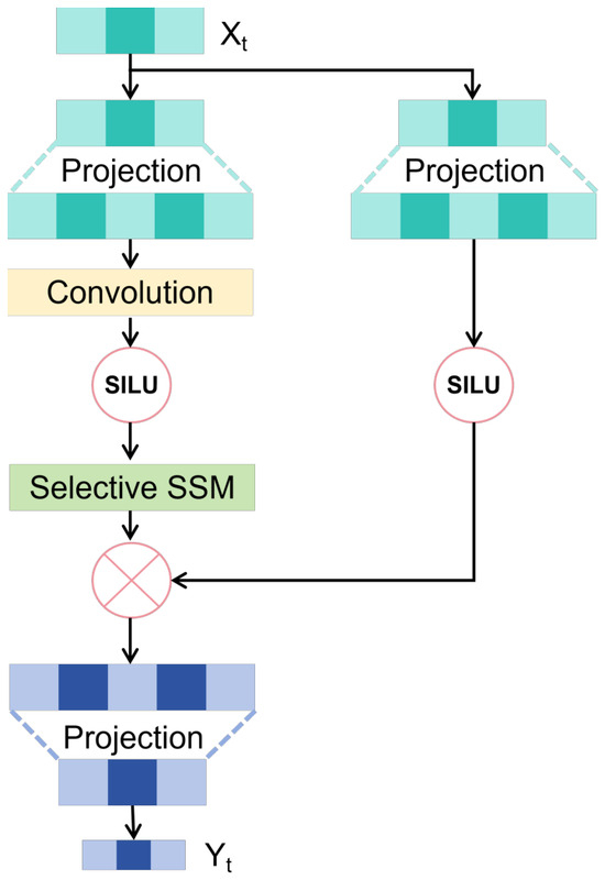
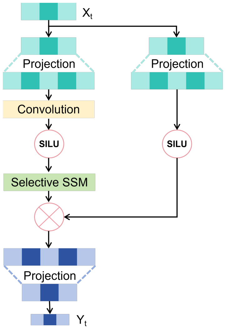
The Mamba model is constructed by stacking multiple Mamba modules (Figure 1), enabling the efficient processing of long-sequence seismic data. Within the main branch of each module, an input sequence $X_t$ is sequentially processed by a multi-layer perceptron (MLP), a convolutional layer, a SILU (Sigmoid Linear Unit) activation function [18], and the selective SSM layer. Residual connections are employed to enhance model stability and performance. Finally, another MLP layer maps the result to the output sequence $Y_t$.

Figure 1. Architecture of the Mamba module. The module contains a main processing branch and a residual branch. Given an input sequence $X_t$, the main branch first applies a multi-layer perceptron (MLP), followed by a convolutional layer, a SiLU (Sigmoid Linear Unit) activation function, and a selective state-space model (selective SSM) layer. The output of the selective SSM is then added to the residual branch to improve training stability and preserve information flow. Finally, another MLP maps the fused features to the output sequence $Y_t$.

In the proposed framework, the selective SSM layer serves as the core operator of the Mamba module for long-sequence modeling. This is particularly suitable for seismic inversion because a seismic trace is essentially a long temporal sequence, and the seismic parameter at a given sample is influenced not only by local reflection details but also by broader contextual information along the time axis. Through recursive state updating, the selective SSM enables effective propagation of informative features over long ranges, which helps the network capture global subsurface parameter trends and long-range dependencies that are difficult to model with purely convolutional operators. Meanwhile, the convolutional branch preserves local waveform patterns and short-range structural variations, which are important for representing reflection details in seismic data. The MLP and SiLU activation further enhance the nonlinear feature transformation ability of the model, allowing more flexible mapping from seismic responses to impedance. Therefore, the Mamba-based DMamUNet provides a suitable mechanism for seismic inversion by jointly modeling long-range temporal context and local seismic characteristics, which is beneficial for improving inversion continuity, trend recovery, and overall prediction accuracy.

2.2. Network Structure and Framework for Seismic Inversion

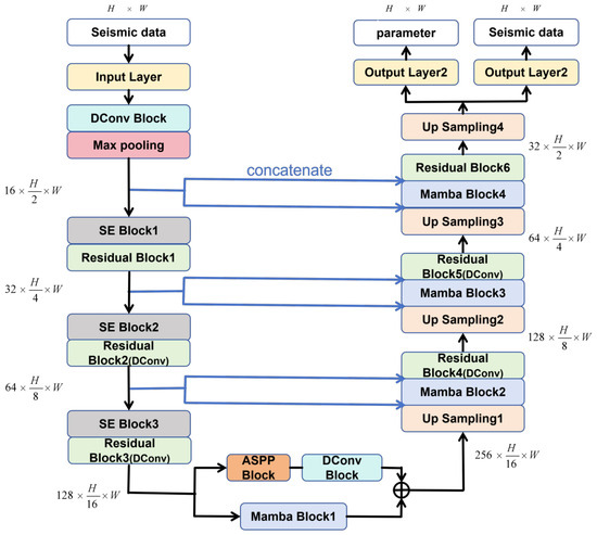
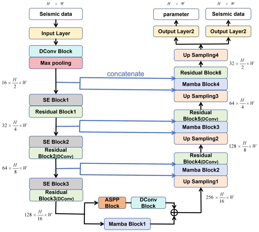
This paper proposes a multi-task seismic inversion network, DMamUNet, based on Mamba modules and a ResUNet++ backbone (Figure 2). The network employs a supervised learning strategy. The network input consists of two-dimensional seismic data with five adjacent traces. To fully exploit the effective information in seismic data and alleviate the challenges posed by limited labeled data, this study introduces an auxiliary task of seismic data reconstruction in addition to the target seismic parameters.

Figure 2. Architecture of the proposed DMamUNet for seismic inversion. The network follows a multi-task encoder–decoder framework with three main parts: an encoder on the left, a bottleneck in the middle, and a decoder on the right. The input consists of two-dimensional seismic data with five adjacent traces. The encoder comprises an input layer, a DConv block, max pooling, and three residual blocks with an SE block. The bottleneck contains parallel ASPP, DConv, and Mamba branches to capture local context and long-range dependencies. The decoder is composed of four upsampling stages. The first three upsampling modules are each composed of an upsampling layer, a Mamba module, and a residual module. The final upsampling module comprises an upsampling layer and a task output layer. Skip connections between the encoder and decoder enable feature fusion across scales, as indicated by the blue arrows.

The overall architecture of DMamUNet comprises three components: the encoder module on the left, the bottleneck module in the middle, and the decoder module on the right.

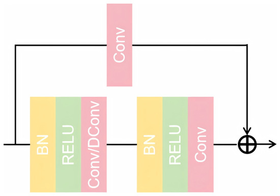
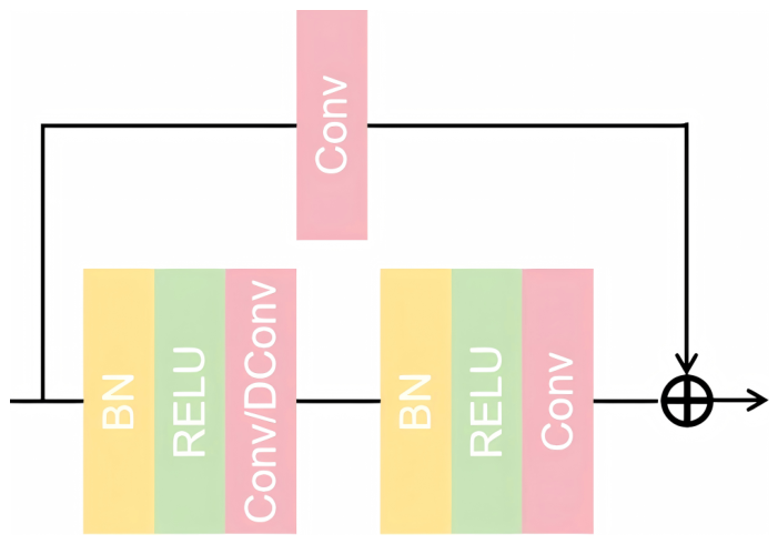
The encoder module primarily consists of an input module, a DConv module, and three residual modules. After seismic data enters the network, it first undergoes feature mapping through the input module, which utilizes residual connection layers to transform seismic data into feature maps. Subsequently, a DConv block (with a kernel size of $5\times 5$) adaptively extracts multi-scale information from the seismic data, followed by max pooling for downsampling the feature maps. The network then performs downsampling through three residual modules (Figure 3). Before each residual module, a Squeeze and Excitation (SE) module [19] is incorporated, which enhances the network’s sensitivity and representational capability for key features by explicitly modeling dependencies between feature channels. The overall encoder performs four downsampling operations to progressively acquire multi-level semantic features from the seismic data.

Figure 3. Architecture of the Residual Block. This block consists of a shortcut branch and a main residual branch with two BN-ReLU-Conv/DConv sub-modules. Conv denotes standard convolution and DConv denotes deformable convolution. The convolution on the shortcut branch is used to align both the channel dimension and spatial resolution with the main branch output, ensuring that the residual addition is valid after downsampling. The outputs of two branches are fused by element-wise addition.

The bottleneck module primarily comprises two parallel branches. One branch consists of an atrous spatial pyramid pooling (ASPP) module and a DConv module for extracting local multi-scale features. The ASPP module contains three parallel dilated convolution layers (with kernel size $3\times 3$ and dilation rates of 6, 12, and 18, respectively). The other branch is a Mamba module specifically designed for modeling long-range dependencies.

The decoder module consists of four upsampling modules. The first three upsampling modules are each composed of an upsampling layer, a Mamba module, and a residual module. The final upsampling module comprises an upsampling layer and a task output layer. The output module stacks four $3\times 3$ convolution layers to ultimately generate the target impedance profiles for five adjacent traces and the reconstructed seismic data.

To facilitate cross-layer information flow and mitigate gradient vanishing problems, the network establishes multiple skip connections between the encoder and decoder, as indicated by the blue arrows in Figure 2. These connections directly transfer shallow high-resolution features generated by the encoder to corresponding levels in the decoder, thereby preserving fine spatial details. For example, feature maps after the first downsampling are concatenated with feature maps after the third upsampling, then input to the fourth Mamba module. The output is further concatenated with feature maps from the first downsampling and fed into the sixth residual module. A similar multi-level feature fusion mechanism permeates the entire network, ensuring effective integration of semantic and spatial information at different scales, ultimately improving the accuracy and stability of seismic inversion results.

2.3. Loss Function and Training Workflow

For loss function, a local mean squared error (MSE) is defined that is computed exclusively between horizons to measure the discrepancy between the predicted results (${\mathbf{y}}^{\prime }$) obtained from seismic data ($\mathbf{x}$) and the ground truth ($\mathbf{y}$). Let Mask denote a binary mask indicating the regions between horizons, and ⊙ represent element-wise multiplication, then

$${\mathcal{L}}_{\mathrm{localMSE}}=\mathbb{E}{\parallel \mathbf{y}\odot \mathrm{Mask}-{\mathbf{y}}^{\prime }\odot \mathrm{Mask}\parallel }_2^2,$$

(8)

where $\mathbb{E}$ denotes the mathematical expectation. Only the valid seismic data between horizons is retained, and the data outside the horizon range is set to zero. Correspondingly, the loss function adopts the masked MSE, which only computes the loss of valid data with values greater than zero.

The overall loss function comprises two components. The total objective function is

$$\mathcal{L}={\mathcal{L}}_{\mathrm{parameter}}+{\mu }_1{\mathcal{L}}_{\mathrm{seis}\_\mathrm{rec}},$$

(9)

where ${\mathcal{L}}_{\mathrm{parameter}}$ denotes the loss between the inversion outputs of five adjacent seismic traces and the interpolated parameter. Furthermore, ${\mathcal{L}}_{\mathrm{seis}\_\mathrm{rec}}$ is the seismic data reconstruction loss, which ensures that the network can effectively learn seismic features. The core advantage of the multi-task framework lies in the high correlation between seismic data and seismic parameters. The framework enables the network to share extracted seismic feature information, fully exploit the internal correlation characteristics between seismic data and parameters, and strengthen the feature representation capability.

For different datasets, corresponding training strategies are adopted. In the Marmousi experiment, since each seismic trace has a corresponding label, a supervised learning procedure is employed. The network parameters are iteratively updated by feeding the training set into the model and minimizing the discrepancy between the predicted and ground-truth values.

In real seismic data experiments, the available labels are limited. To overcome this issue, this paper adopts a “pre-training and fine-tuning” transfer learning strategy [4], which consists of two steps.

(1)

Pre-training: Synthetic data with distributions similar to real seismic data and their corresponding impedance labels are constructed to pre-train the model for acquiring initial inversion capabilities. The loss function used in pre-training follows Equation (9).

(2)

Fine-tuning: The pre-trained model serves as the initial model, which is then fine-tuned using field seismic data and interpolated impedance to improve generalization. The fine-tuning stage continues to employ Equation (9) for optimization.

3. Results

3.1. Synthetic Marmousi Model Experiment

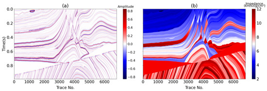
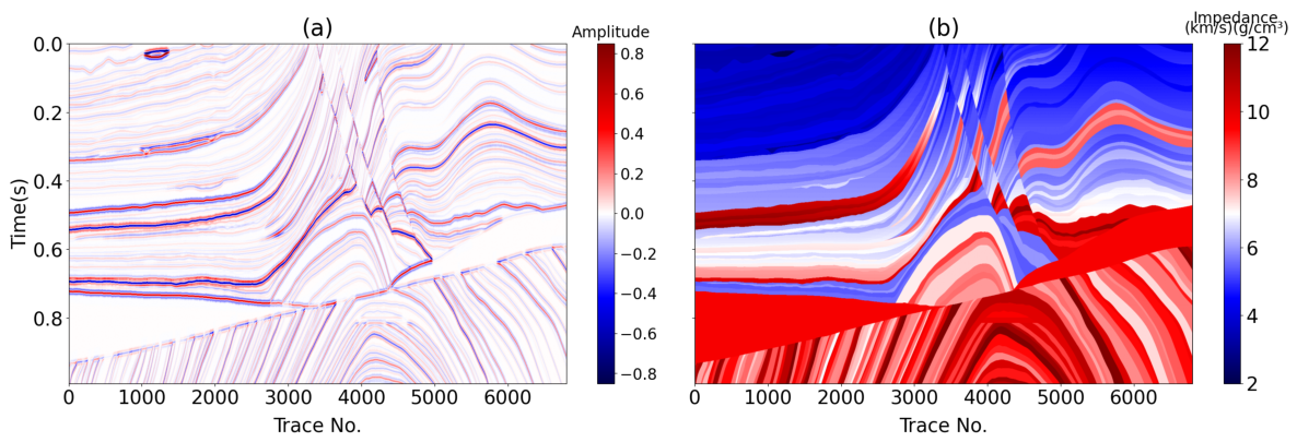
The effectiveness of DMamUNet is first validated using the downsampled Marmousi model [20]. To synthesize realistic seismic records, we convolve the reflectivity series of the Marmousi model with a Ricker wavelet, where the dominant frequency is randomly generated within the range of 25–35 Hz. The resulting dataset, illustrated in Figure 4, comprises 6800 traces, each consisting of 1000 sampling points at a 1 ms interval. For the training phase, a subset consisting of 68 trace pairs is extracted at equidistant intervals, accounting for 1% of the entire dataset. During training, we employ the Adam optimizer with the learning rate of 0.0005, the weight decay of $1\times {10}^{-6}$, the batch size of 3, and training for 1000 epochs.

Figure 4. Marmousi model dataset. (a) Synthetic seismic data. (b) True Impedance.

In this experiment, we select FCRN [21] and TransUNet [22] as baseline methods for comparison with our proposed DMamUNet. To ensure a fair comparison, all methods adopt the multitrace-to-multitrace strategy and are configured with identical hyperparameters.

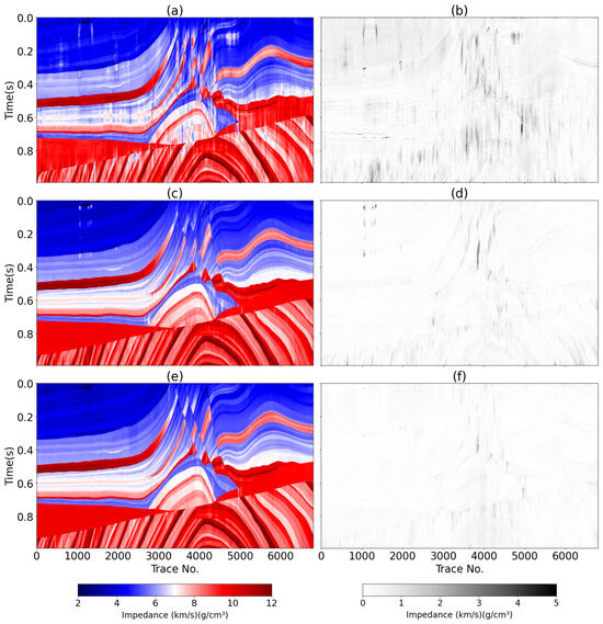
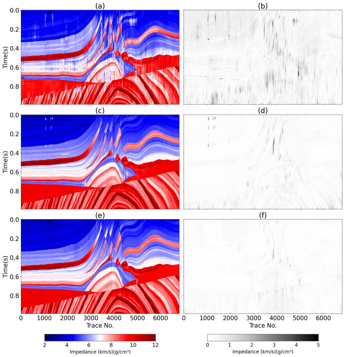
As illustrated in Figure 5, panels (a), (c) and (e) present the impedance inversion results of FCRN, TransUNet and DMamUNet, respectively, while panels (b), (d) and (f) display the corresponding absolute errors. FCRN yields the poorest inversion performance among the three methods. Its result is plagued by pervasive artifacts, weak lateral continuity and low resolution, and fails to accurately characterize fine stratigraphic structures. TransUNet achieves moderate improvements over FCRN, with mitigated artifacts and better stratigraphic continuity. Nevertheless, notable artifacts still persist in the upper-left region and the central complex zones with drastic stratigraphic structural changes. In contrast, DMamUNet delivers the optimal inversion quality, with substantially enhanced accuracy and lateral continuity, particularly in the complex fault zones in the middle and upper sections of the profile.

Figure 5. Impedance prediction results for the Marmousi model: (a) FCRN, (c) TransUNet, (e) DMamUNet. (b–f) Alongside are the corresponding absolute error profiles.

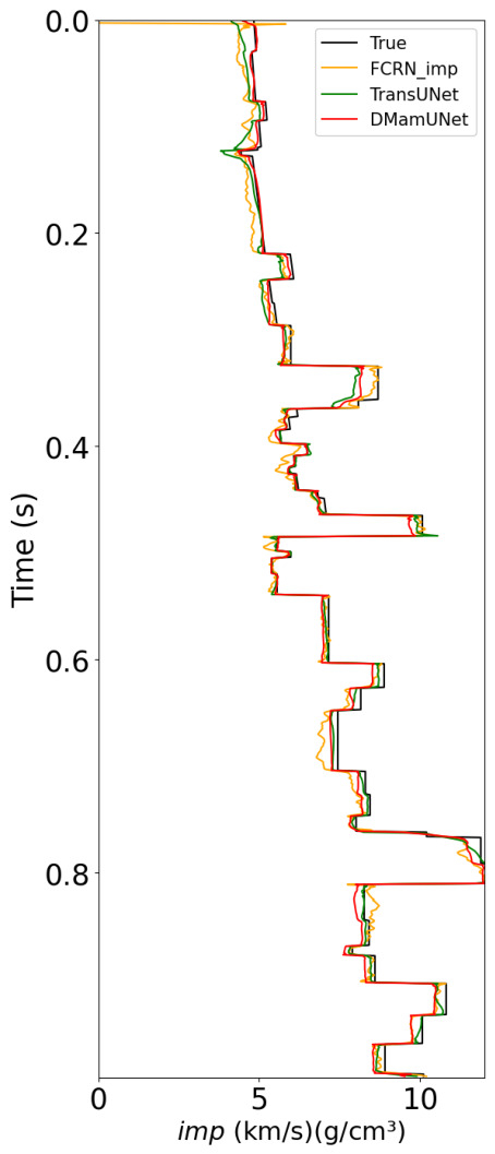
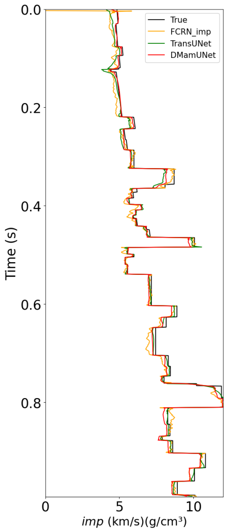
The error maps further corroborate these observations. FCRN presents the largest overall error values across the profile, while TransUNet reduces the error magnitude to a certain extent. DMamUNet produces the smallest errors with significantly suppressed artifacts. Figure 6 provides a comparison of trace 3505, highlighting the superior alignment between our inversion result (red) and the ground truth (black).

Figure 6. Comparison of FCRN, TransUNet, and DMamUNet inversion results at synthetic trace 3505, with label values on the synthetic data.

Finally, we quantify the inversion performance by calculating the mean squared error (MSE), Pearson correlation coefficient (PCC) and coefficient of determination ($R^2$) between the predicted profiles and the true impedance model, with the results listed in Table 1. Quantitative results demonstrate that DMamUNet consistently outperforms both FCRN and TransUNet across all evaluation metrics, achieving the lowest MSE as well as the highest PCC and $R^2$.

Table 1. Quantitative analysis of inversion results for the Marmousi model (best results are highlighted in bold).

Model	PCC	MSE	${\mathbf{R}}^2$
FCRN	0.9714	0.3870	0.9194
TransUNet	0.9944	0.0735	0.9837
DMamUNet	0.9976	0.0410	0.9908

3.2. Field Data Experiment

3.2.1. Field Post-Stack Data Experiment

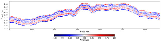
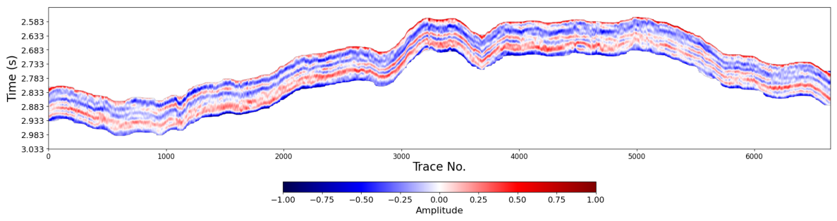
To further validate the performance of DMamUNet, we apply it to real post-stack seismic data, which consists of 6647 traces and 10 wells with 5531 sampling points and a time sampling interval of 0.1 ms (Figure 7). To augment the data, this study performs interpolation on the impedance and seismic data. Subsequently, synthetic seismic data is generated using the interpolated impedance. In the pre-training stage, the network is trained using synthetic seismic data and corresponding interpolated impedance data. A total of 210 traces surrounding wells are selected as labeled data, with a training-to-validation ratio of 9:1. The value ${\mu }_1$ is selected by trial as 1. In the fine-tuning stage, the network is trained using interpolated seismic data and interpolated impedance data, with W3 designated as the blind well. The parameters remain consistent with the pre-training stage.

Figure 7. Cross-well seismic profile of the field post-stack data.

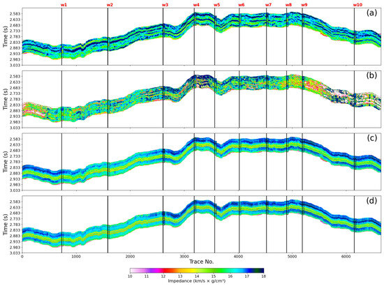
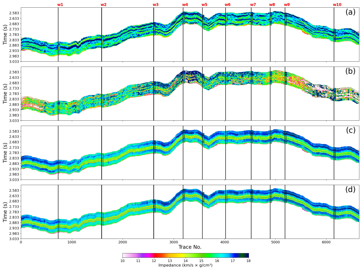
The impedance inversion results generated by the conventional constrained sparse spike inversion (CSSI), FCRN, TransUNet, and our proposed DMamUNet are displayed in Figure 8, where panels (a) to (d) correspond to the four methods, respectively.

Figure 8. Impedance prediction results for the field post-stack data: (a) CSSI, (b) FCRN, (c) TransUNet, (d) DMamUNet. (Well W3 serves as blind well).

The CSSI result generally suffers from low vertical resolution, leading to poor consistency with the true well-log values at well locations. As for the FCRN result, it contains abundant abnormal values and exhibits discontinuous stratigraphic features with low overall resolution, failing to effectively depict the detailed lateral variations of impedance. In comparison, the TransUNet result achieves overall improvement in inversion quality. Nevertheless, it still has insufficient vertical resolution, and its lateral continuity is evidently inferior to that of DMamUNet. By contrast, the inversion result produced by DMamUNet is more consistent with the stratigraphic configuration reflected in the seismic data, and is capable of recovering richer and more detailed structural information. Moreover, compared with CSSI, FCRN and TransUNet, DMamUNet yields significant improvements in both lateral and vertical resolution.

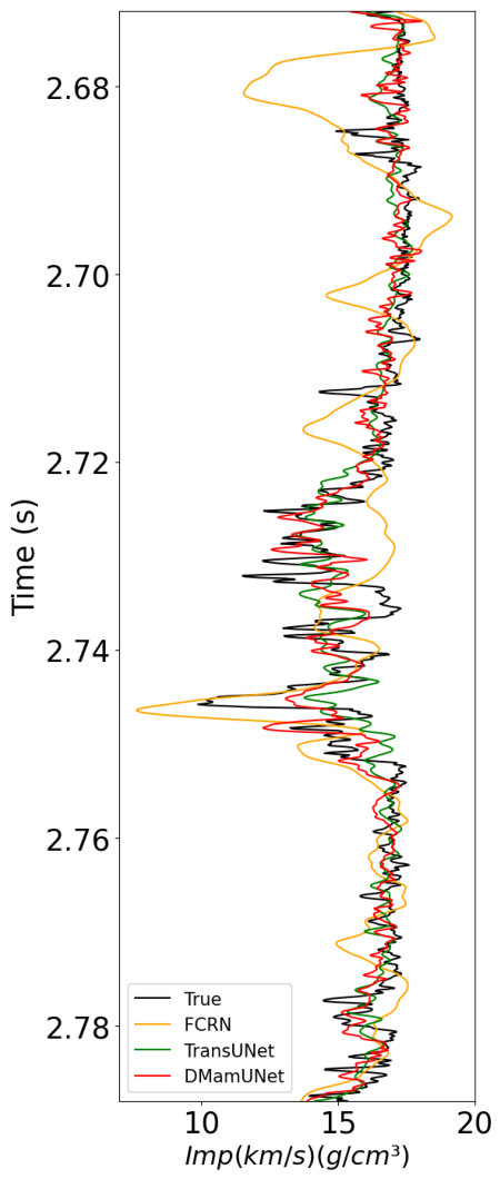
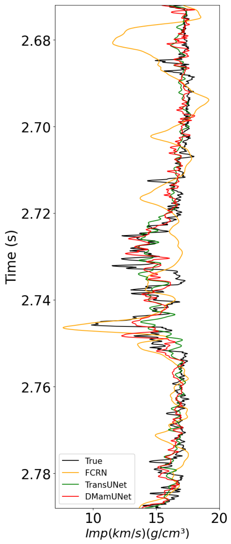
Figure 9 shows the blind well W3 log comparison of FCRN, TransUNet and DMamUNet against the ground-truth well curve. The FCRN prediction presents the largest overall deviation from the true values, while TransUNet and DMamUNet produce predictions much closer to the ground truth. Among the three deep learning methods, DMamUNet achieves the highest consistency with the true well-log data.

Figure 9. Comparison of FCRN, TransUNet, and DMamUNet inversion results in the blind well W3 with label values on the field post-stack data.

Quantitative evaluation at the blind well W3 is presented in Table 2, with the MSE, PCC, and $R^2$ adopted as evaluation metrics. For DMamUNet, the PCC and $R^2$ between the inverted results and the true well-log curve reach 0.9980 and 0.9958, respectively, while the MSE is 0.1898, indicating a substantial improvement in inversion fidelity. These results demonstrate that DMamUNet has strong seismic feature extraction capability and global impedance modeling ability, thereby effectively improving the accuracy and resolution of post-stack multi-task inversion.

Table 2. Quantitative analysis of inversion results for blind well W3 (best results are highlighted in bold).

Model	PCC	MSE	${\mathbf{R}}^2$
FCRN	0.9905	0.8716	0.9808
TransUNet	0.9976	0.2207	0.9951
DMamUNet	0.9980	0.1898	0.9958

3.2.2. Field Pre-Stack Data Experiment

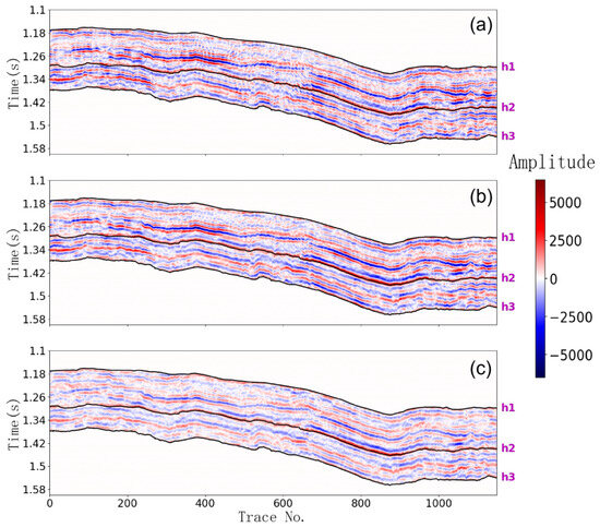
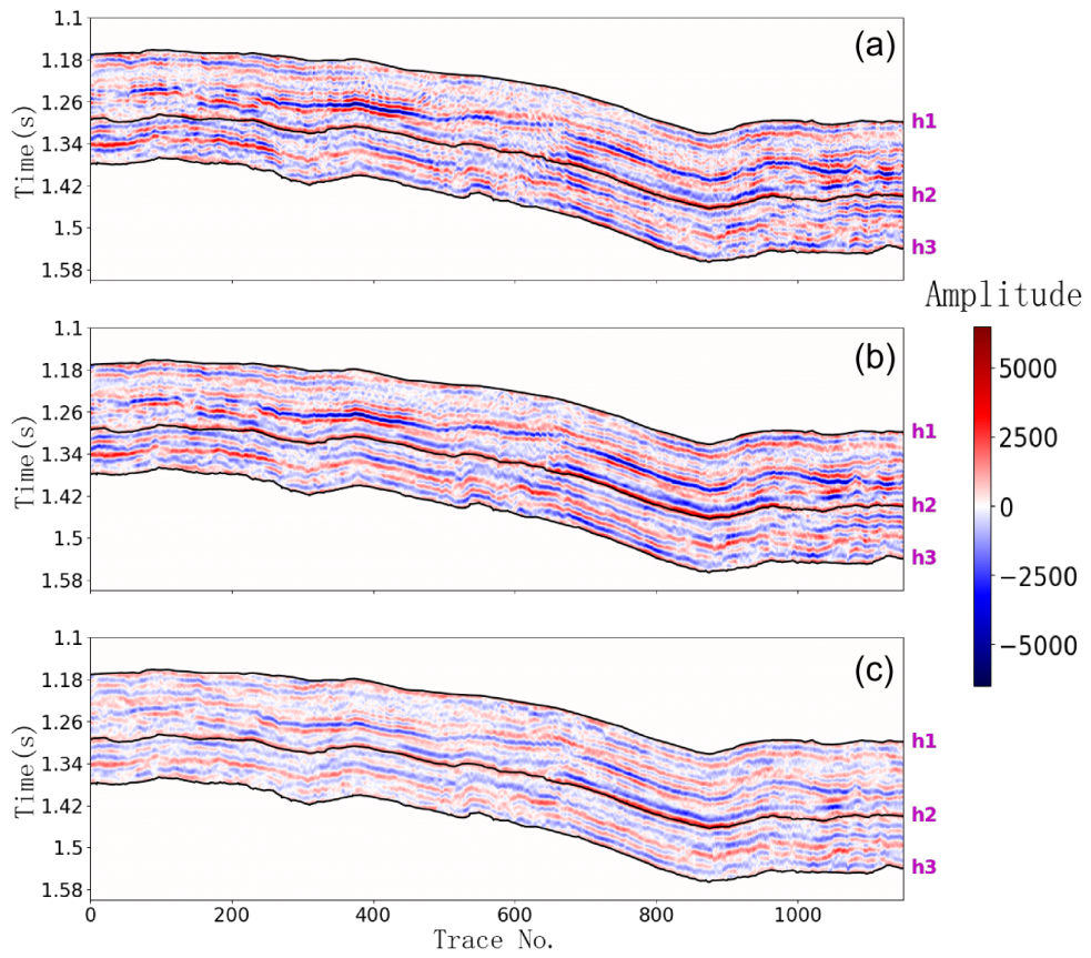
To further validate the performance of the proposed DMamUNet in seismic inversion, we applied it to actual 3D pre-stack seismic data. The dataset includes three angle volumes at 9°, 22°, and 34°, and Figure 10 displays the seismic profiles passing through wells for different angles. The multi-angle seismic data are concatenated along the channel dimension to form a multi-channel input tensor. This strategy allows the network to effectively integrate and jointly learn complementary structural and petrophysical information from different incidence angles, facilitating a more robust characterization of the subsurface seismic-geological features. Each data volume has dimensions of 921 (Inline) × 991 (Crossline) × 701 (Timeline), totaling 921,711 seismic traces, with each trace consisting of 701 time samples at a sampling interval of 1 ms. The dataset contains four wells (W1–W4), where W1 and W2 have known values for all three elastic parameters (P-wave velocity $V_p$, S-wave velocity $V_s$, and density $\rho$), W3 provides information for $V_p$ and $\rho$, and W4 only provides $V_p$ information. Model training utilized only data from wells W1 and W2, with the available parameters on W3 and W4 serving as blind well validation.

Figure 10. Pre-stack seismic data at three incidence angles from the field dataset. The figure displays seismic amplitude profiles at incidence angles of (a) 9°, (b) 22°, (c) 34°.

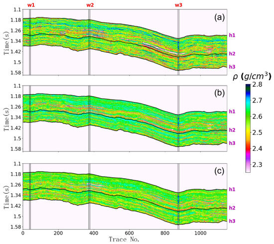
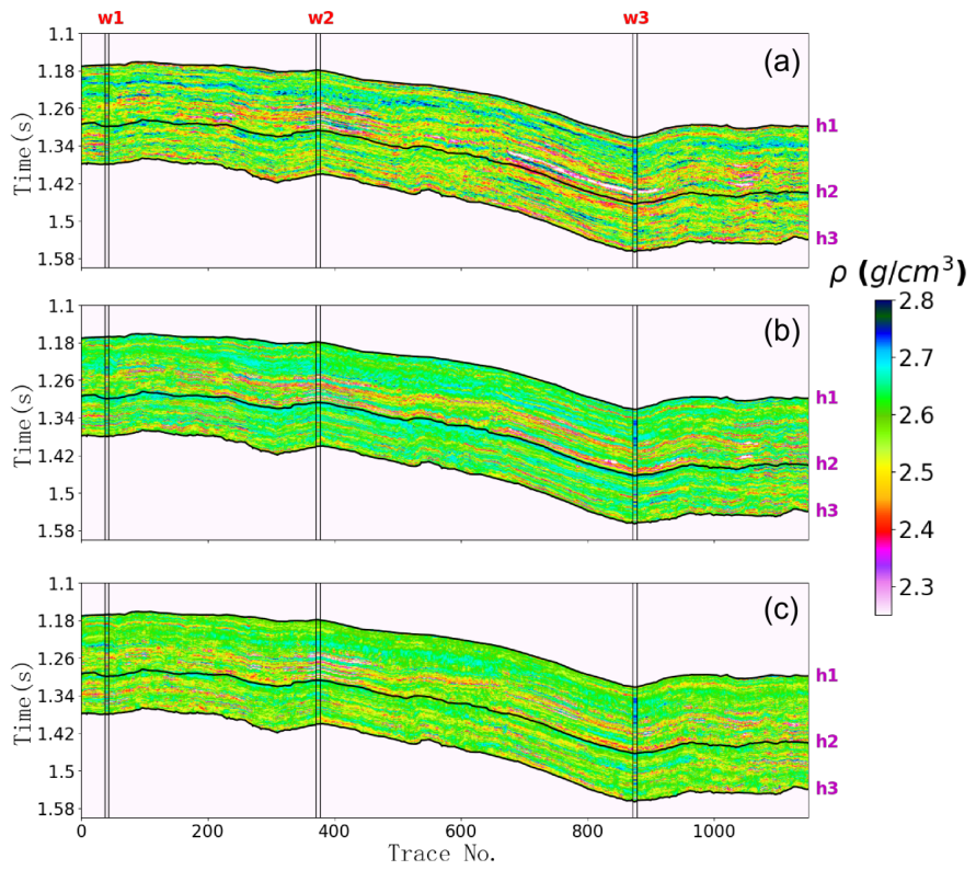
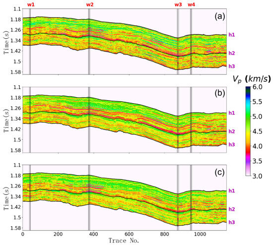
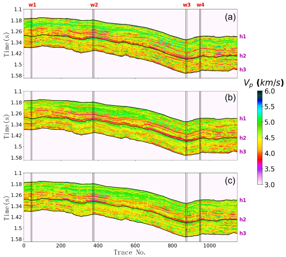
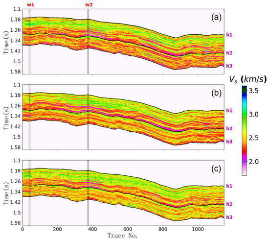
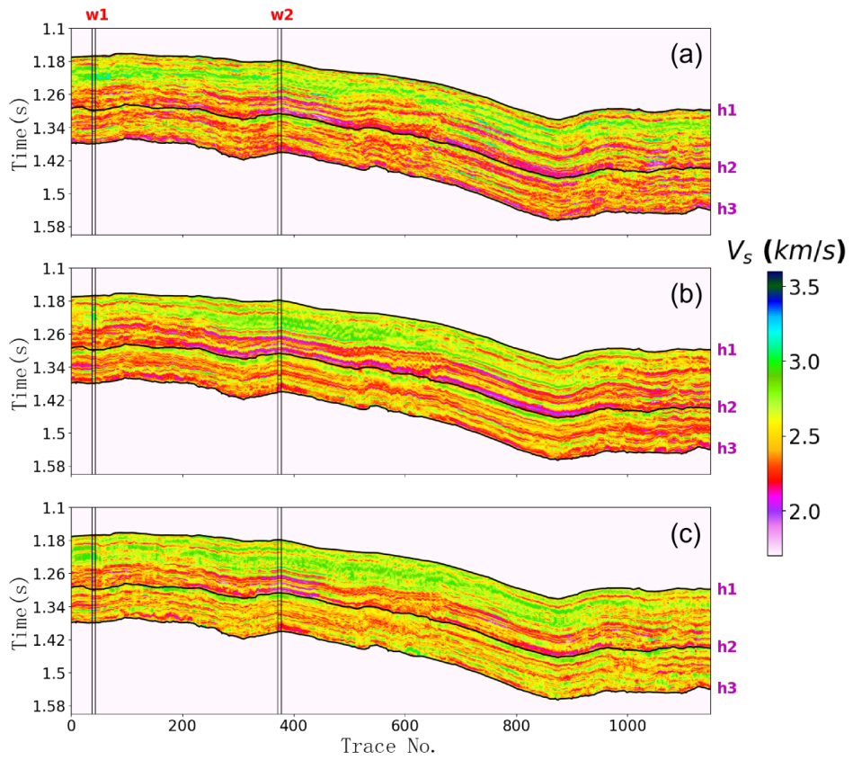
Figure 11, Figure 12 and Figure 13 present the comparison results of different methods for the three parameters. The inversion results from DMamUNet not only show high agreement with the training wells but also exhibit good matching with the blind wells (W3 and W4). Additionally, the entire cross-well profiles demonstrate strong lateral continuity, and the inverted stratigraphy is consistent with the structural features observed in the seismic data. Furthermore, the method successfully retrieves numerous thin layers that were not identified by other comparative methods.

Figure 11. Inversion results of density ($\rho$) on field data: (a) FCRN, (b) TransUNet, (c) DMamUNet.

Figure 12. Inversion results of P-wave velocity ($V_p$) on field data: (a) FCRN, (b) TransUNet, (c) DMamUNet.

Figure 13. Inversion results of S-wave velocity ($V_s$) on field data: (a) FCRN, (b) TransUNet, (c) DMamUNet.

FCRN yields low-resolution results for $V_p$ and $V_s$, and its $\rho$ inversion shows poor lateral continuity with many outliers. TransUNet also produces lower-resolution results for $V_p$ and $V_s$ compared with DMamUNet, and its $\rho$ inversion result at the blind well location is inferior to those of DMamUNet.

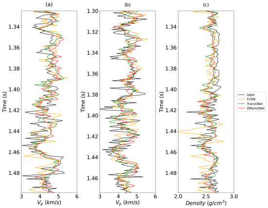
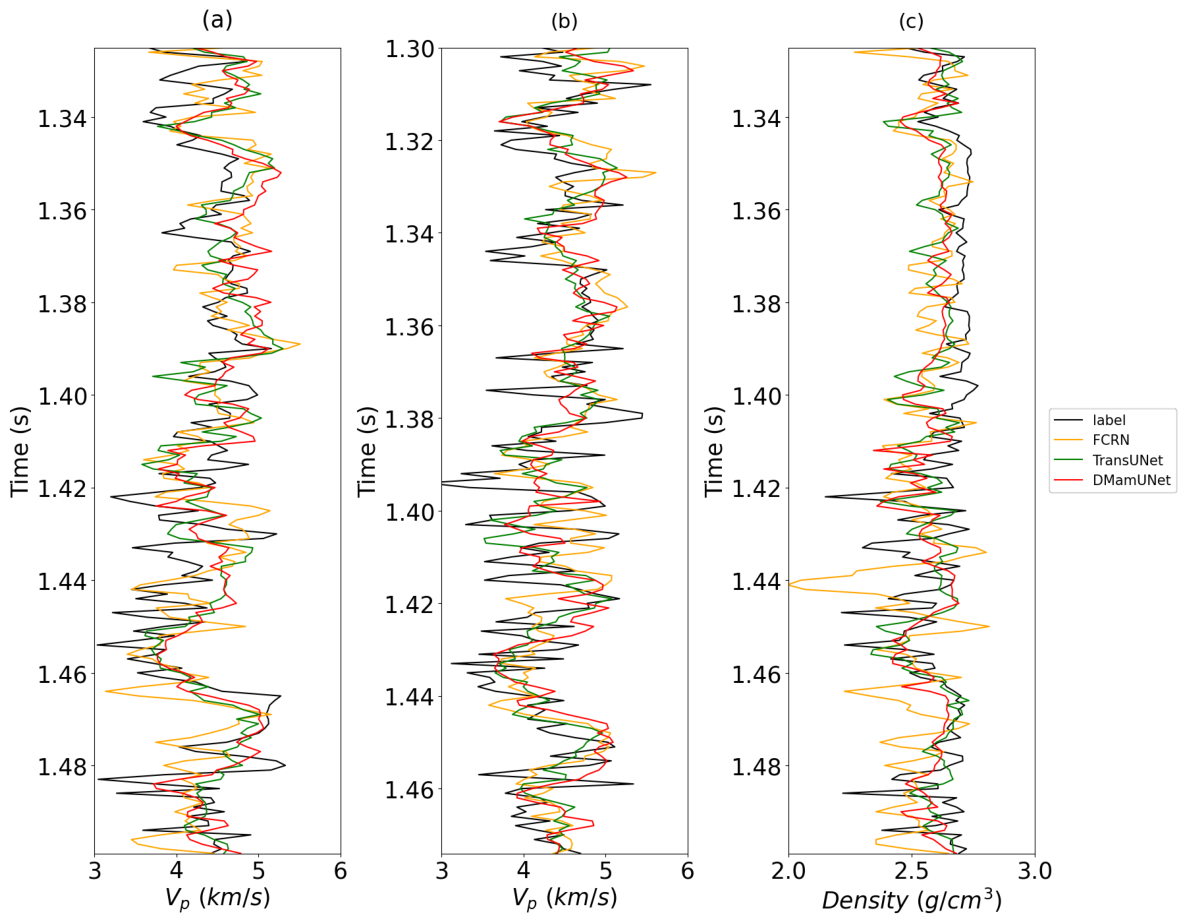
As illustrated in Figure 14, comparative validation across two blind wells (W3 and W4) confirms that DMamUNet achieves excellent generalization performance and prediction accuracy in both P-wave velocity ($V_p$) and density inversion tasks. Compared with FCRN, which produces pronounced deviations at anomalous intervals, and TransUNet, which exhibits limited ability to capture fine-scale details, DMamUNet reproduces the fluctuation patterns of formation well-log curves with greater precision. It delivers particularly strong robustness and stability when handling abrupt stratigraphic changes and complex local features, verifying its remarkable advantages in multi-physical property well-log data inversion tasks.

Figure 14. Comparison of FCRN, TransUNet, and DMamUNet inversion results in the blind well with label values on the field pre-stack data: (a) $V_p$ in blind well W3, (b) $V_p$ in blind well W4, (c) density in blind well W3.

Finally, Table 3 lists the mean squared error (MSE) and Pearson correlation coefficient (PCC) of the prediction results for the blind wells W3 and W4 using various methods. For $V_p$ prediction, DMamUNet achieves the best performance in all metrics except for a slightly higher MSE than TransUNet at W4. For $\rho$ prediction, DMamUNet delivers the lowest MSE (0.005072) and the highest PCC (0.998509) among all methods.

Table 3. Quantitative indicators of inversion results for three parameters versus true values for methods at W3 and W4 (optimal results are displayed in bold. Note: No S-wave velocity data for blind well validation).

Method	P-Wave Velocity				Density
	W3		W4		W3
	MSE	PCC	MSE	PCC	MSE	PCC
FCRN	0.108327	0.987779	0.110496	0.988231	0.009756	0.997388
TransUNet	0.097572	0.989858	0.092631	0.989844	0.005268	0.998362
DMamUNet	0.096558	0.991248	0.098843	0.990027	0.005072	0.998509

4. Discussion

A comprehensive discussion of the proposed DMamUNet model is provided from four perspectives: ablation experiments, data processing and experimental details, computational efficiency, and comprehensive analysis and discussion.

4.1. Ablation Experiments

To evaluate the contribution of each component within our proposed architecture, we perform a comprehensive ablation study on post-stack seismic data.

4.1.1. Baseline Comparison (ResUNet++)

First, ResUNet++, which integrates residual convolution, SE blocks, ASPP modules and the traditional attention block, is adopted as the baseline model in this work. Since its structural design has been fully validated in existing studies, additional individual ablation tests on its internal modules are unnecessary. Quantitative evaluation on blind wells shows that ResUNet++ yields an MSE of 0.4195, an $R^2$ of 0.9908 and a PCC of 0.9957. All these metrics are inferior to those of the proposed DMamUNet, which preliminarily verifies the superiority of the structural improvements embedded in our model.

4.1.2. Mamba vs. Transformer Module

To further validate the effectiveness of the core modules in DMamUNet, controlled contrast experiments are conducted under identical network architectures, where only the Mamba modules at the decoder and bottleneck layers are replaced with MHSA modules. We compare the reconstruction accuracy and computational efficiency of the two variants. In terms of accuracy, the Transformer-based model achieves a PCC of 0.9987, an MSE of 0.14 and an $R^2$ of 0.9968 on the blind well, whereas DMamUNet obtains the same PCC of 0.9990, a lower MSE of 0.09 and a higher $R^2$ of 0.9979. In terms of computational cost, the Transformer-based model consumes 30 min 44.5 s (pre-training) and 41.9 min (fine-tuning) for training, accompanied by a high GPU memory occupation of 16,870 MiB. By contrast, DMamUNet only takes 28 min 39.9 s (pre-training) and 36.7 min (fine-tuning) for training, with a memory usage of merely 3298 MiB. These results sufficiently demonstrate that the Mamba module outperforms the conventional Transformer module in both reconstruction accuracy and computational efficiency for seismic inversion tasks.

It should be noted that the above module comparison experiments are implemented using a subset of 1700 seismic traces. When the full dataset consisting of 6647 seismic traces is fed into the network, the Transformer-based model encounters out-of-memory errors. To guarantee the normal execution of experiments, only the deformable convolutions inside residual blocks are substituted with standard convolutions while keeping the rest of the network unchanged. This phenomenon further reveals the poor scalability and excessive memory overhead of the Transformer architecture when training on large-scale seismic datasets.

4.1.3. M2M Strategy

From the perspective of training strategy optimization, the effectiveness of the proposed M2M strategy is verified via comparisons with the classic multitrace-to-single-trace (M2S) strategy proposed in the published literature. Blind-well tests show that the MSE of the M2M strategy is 0.1898, lower than the MSE of 0.1939 achieved by the M2S strategy, confirming that the M2M strategy can effectively improve seismic inversion accuracy.

4.1.4. Seismic Reconstruction Loss Weight

For the weight selection of the seismic reconstruction in the loss function, ablation experiments are carried out with five weight values: 0, 0.2, 0.5, 1.0 and 1.5, corresponding to blind well MSE values of 0.1635, 0.2495, 0.2103, 0.1898 and 0.2163, respectively. Although the model with a weight of 0 achieves slightly better blind well accuracy, it suffers from severe fitting errors on training wells. For example, the MSE of well W2 reaches 0.2688 under the zero-weight setting, while the MSE of well W2 predicted by DMamUNet with a weight of 1.0 is only 0.0047. Considering the overall fitting performance on both blind wells and training wells comprehensively, the optimal weight of 1.0 is finally adopted for the seismic reconstruction loss term and applied to all subsequent experiments. For pre-stack multi-parameter inversion experiments, identical weight coefficients are assigned to each seismic parameter owing to their equal contributions to final reconstruction results.

4.1.5. Transfer Learning

We also verified the effect of transfer learning. Without transfer learning, the blind well MSE is 0.2519, while the value drops to 0.1898 after introducing transfer learning. This result confirms that transfer learning effectively improves the inversion performance of the model.

4.2. Data Processing and Experimental Details

Horizon data used in this study are manually picked. Min–Max Scaling is utilized for data normalization and seismic data are scaled to the range $[-1,1]$, while label data are normalized to $[0,1]$. Different from the traditional sliding-window input paradigm, the network receives complete time-series information of five consecutive seismic traces as input and outputs inversion results for the corresponding five traces, which preserves the integrity of spatiotemporal seismic features and guarantees lateral spatial continuity.

Based on horizon data, well-logging data and raw seismic data, Kriging interpolation is adopted to generate interpolated impedance data and interpolated seismic data. Synthetic seismic traces are further produced by convolving the statistical wavelet extracted from real field data with interpolated impedance. No blind well information is involved in the entire data processing workflow to avoid data leakage.

To align the data distribution between synthetic and real seismic data, we adopt two core measures. First, we apply the identical Min-Max normalization scheme to both datasets, scaling all amplitude values to the range of $[-1,1]$ to unify their numerical ranges. Second, since the interpolated impedance profile is generated under real geological constraints from training wells and field horizons, its stratigraphic structure, impedance value range and lateral variation trend are highly consistent with actual subsurface conditions. Accordingly, the synthetic seismic data generated from this impedance profile naturally share highly similar amplitude distribution, spectral characteristics and geological structural features with real field seismic data. On this basis, the subsequent fine-tuning process further adapts the model to subtle distribution differences in real field data, ensuring effective knowledge transfer from synthetic pre-training to field data applications.

To ensure the reproducibility and stability of all experimental results, the random seed is fixed to 8 by executing random.seed(8) throughout the experiments.

4.3. Computational Efficiency

The number of trainable parameters, training time and inference latency of all competing models are statistically quantified. FCRN has 122,868 trainable parameters, TransUNet has 225,767, and the proposed DMamUNet has 4,023,364. All experiments are conducted on an NVIDIA GeForce RTX 3090 GPU with a total memory capacity of 24,576 MiB. In terms of per-epoch training time, FCRN consumes 0.056 s, TransUNet consumes 0.209 s, and DMamUNet consumes 0.268 s. Regarding total inference time on the post-stack field seismic dataset, FCRN takes 1 min 44 s, TransUNet takes 13 min 59 s, and DMamUNet takes 15 min 03 s.

Under identical training and prediction pipelines, the proposed DMamUNet requires slightly longer training and inference time than TransUNet due to the introduction of deformable convolutions. Future work will focus on lightweight convolution optimization and other relevant directions to further reduce computational overhead and improve practical deployment efficiency of the seismic inversion algorithm.

4.4. Comprehensive Analysis and Discussion

In this study, the performance of the proposed DMamUNet was systematically evaluated across three hierarchical levels of experimental data. The synthetic data experiments established the baseline for the model’s fundamental inversion capabilities. Subsequent tests on post-stack data confirmed its precision in tracking stratigraphic trends within real seismic contexts. Finally, pre-stack data experiments pushed the model to its limits, challenging its ability to process complex physical attributes and noise-sensitive signals. Across all these experimental configurations, DMamUNet consistently outperformed the benchmark models (FCRN and TransUNet), providing more reliable and physically plausible inversion results.

However, it is important to acknowledge certain limitations. Specifically, while the model demonstrates robust performance, its predictive accuracy in pre-stack blind well validation shows a relatively higher degree of uncertainty compared to post-stack results. This discrepancy is largely attributed to the inherent complexity of pre-stack seismic data, which is highly sensitive to random noise and requires sophisticated handling of non-unique solutions in AVO inversion. Although DMamUNet captures the primary geological trends successfully, the subtle high-frequency variations in the pre-stack domain remain a challenging bottleneck. This underscores the potential for future research to incorporate physics-informed constraints (e.g., integrating rock physics models into the loss function) to further bridge the performance gap and enhance the resolution of fine-scale stratigraphic features.

5. Conclusions

This paper presents DMamUNet, a deep learning network that incorporates the Mamba model for multitask seismic inversion. By integrating DConv and Mamba modules into the ResUNet++ backbone, DMamUNet effectively overcomes the trade-off between local feature extraction and long-range seismic sequence modeling. The architecture captures high-frequency stratigraphic details while simultaneously reconstructing the low-frequency impedance trends, which is critical for both post-stack acoustic impedance inversion and pre-stack multi-parameter (Vp, Vs, and density) estimation. The model’s robustness is further enhanced through a composite loss combining well-log parameter supervision with seismic reconstruction and the multitrace-to-multitrace inversion strategy. A pre-training and fine-tuning transfer learning approach is also employed to address the challenge of limited well-log data. Experimental results on synthetic and field datasets demonstrate that DMamUNet consistently outperforms existing architectures, particularly in recovering vertical impedance variations in post-stack data and maintaining physical consistency among multiple elastic parameters in pre-stack inversion.

References

- Lin, Y.; Peng, S.; Cui, X.; Lu, Y. Post-stack seismic impedance inversion based on sparse-coded Mamba seismic model. Phys. Chem. Earth 2025, 141, 104114. [Google Scholar] [CrossRef] [Scilit]
- Mousavi, S.M.; Beroza, G.C. Deep-learning seismology. Science 2022, 377, eabm4470. [Google Scholar] [CrossRef] [Scilit] [PubMed]
- Adler, A.; Araya-Polo, M.; Poggio, T. Deep learning for seismic inverse problems: Toward the acceleration of geophysical analysis workflows. IEEE Signal Process. Mag. 2021, 38, 89–119. [Google Scholar] [CrossRef] [Scilit]
- Wu, B.; Xie, Q.; Wu, B. Seismic impedance inversion based on residual attention network. IEEE Trans. Geosci. Remote Sens. 2022, 60, 4511117. [Google Scholar] [CrossRef] [Scilit]
- Song, C.; Lu, W.; Geng, W.; Duan, X.; Wang, Y.; Wang, Q.; Ma, Q.; Li, Y. A review of seismic impedance inversion methods based on physics-informed neural network. Geophys. Prospect. Pet. 2025, 64, 595–621. [Google Scholar] [CrossRef]
- Fu, J.; Fan, R.; Cao, J.; Zhang, X.; Shi, S. Seismic impedance inversion using a joint deep learning model based on convolutional neural network and Transformer. IEEE J. Sel. Top. Appl. Earth Obs. Remote Sens. 2023, 16, 8913–8922. [Google Scholar] [CrossRef] [Scilit]
- Alfarraj, M.; Alregib, G. Semisupervised sequence modeling for elastic impedance inversion. Interpretation 2019, 7, SE237–SE249. [Google Scholar] [CrossRef] [Scilit]
- Guo, R.; Zhang, J.J.; Liu, D.; Zhang, Y.B.; Zhang, D.W. Application of bi-directional long short-term memory recurrent neural network for seismic impedance inversion. In Proceedings of the 81st EAGE Conference and Exhibition, London, UK, 3–6 June 2019; pp. 1–5. [Google Scholar] [CrossRef] [Scilit]
- Wang, J.; Cao, J.X. Data-driven S-wave velocity prediction method via a deep-learning-based deep convolutional gated recurrent unit fusion network. Geophysics 2021, 86, M185–M196. [Google Scholar] [CrossRef] [Scilit]
- Song, L.; Yin, X.Y.; Zong, Z.Y.; Jiang, M. Semi-supervised learning seismic inversion based on spatio-temporal sequence residual modeling neural network. J. Pet. Sci. Eng. 2022, 208, 109549. [Google Scholar] [CrossRef] [Scilit]
- Vaswani, A.; Shazeer, N.; Parmar, N.; Uszkoreit, J.; Jones, L.; Gomez, A.N.; Kaiser, Ł.; Polosukhin, I. Attention is all you need. In Proceedings of the 31st International Conference on Neural Information Processing Systems (NIPS), Long Beach, CA, USA, 4–9 December 2017; Curran Associates, Inc.: Red Hook, NY, USA, 2017; pp. 5998–6008. [Google Scholar]
- Ning, C.; Wu, B.; Zhu, Z. Transformer and CNN hybrid neural network for seismic impedance inversion. In Proceedings of the IGARSS 2023–2023 IEEE International Geoscience and Remote Sensing Symposium; IEEE: Piscataway, NJ, USA, 2023; pp. 5543–5546. [Google Scholar] [CrossRef] [Scilit]
- Gu, A.; Dao, T. Mamba: Linear-time sequence modeling with selective state spaces. arXiv 2024, arXiv:2312.00752. [Google Scholar]
- Jha, D.; Smedsrud, P.H.; Riegler, M.A.; Johansen, D.; Lange, T.D.; Halvorsen, P.; Johansen, H.D. ResUNet++: An advanced architecture for medical image segmentation. In Proceedings of the 2019 IEEE International Symposium on Multimedia (ISM); IEEE: Piscataway, NJ, USA, 2019; pp. 225–255. [Google Scholar] [CrossRef] [Scilit]
- Wang, W.; Dai, J.; Chen, Z.; Huang, Z.; Li, Z.; Zhu, X.; Hu, X.; Lu, T.; Lu, L.; Li, H.; et al. InternImage: Exploring large-scale vision foundation models with deformable convolutions. In Proceedings of the IEEE/CVF Conference on Computer Vision and Pattern Recognition (CVPR), Vancouver, BC, Canada, 18–22 June 2023; pp. 14408–14419. [Google Scholar]
- Luo, Y.; Liu, X.; Meng, H.; Ye, Y.; Wu, B. Multitask seismic inversion based on deformable convolution and generative adversarial network. IEEE Geosci. Remote Sens. Lett. 2024, 21, 1–5. [Google Scholar] [CrossRef] [Scilit]
- Zheng, Q.; Wei, C.; Yan, X.; Ruan, H.; Wu, B. Seismic elastic parameter inversion via a FCRN and GRU hybrid network with multi-task learning. Appl. Sci. 2023, 13, 10519. [Google Scholar] [CrossRef] [Scilit]
- Elfwing, S.; Uchibe, E.; Doya, K. Sigmoid-weighted linear units for neural network function approximation in reinforcement learning. Neural Netw. 2018, 107, 3–11. [Google Scholar] [CrossRef] [Scilit] [PubMed]
- Hu, J.; Shen, L.; Sun, G. Squeeze-and-Excitation networks. In Proceedings of the IEEE/CVF Conference on Computer Vision and Pattern Recognition (CVPR), Salt Lake City, UT, USA, 18–22 June 2018; pp. 7132–7141. [Google Scholar] [CrossRef] [Scilit]
- Martin, G.S.; Wiley, R.; Marfurt, K.J. Marmousi2: An elastic upgrade for Marmousi. Lead. Edge 2006, 25, 156–166. [Google Scholar] [CrossRef] [Scilit]
- Wang, L.; Meng, D.; Wu, B. Seismic inversion via closed-loop fully convolutional residual network and transfer learning. Geophysics 2021, 86, R671–R683. [Google Scholar] [CrossRef] [Scilit]
- Peng, Z.; Xu, H. Post-stack seismic impedance inversion method based on TransUNet neural network. Prog. Geophys. 2024, 39, 704–715. [Google Scholar] [CrossRef]
Disclaimer/Publisher’s Note: The statements, opinions and data contained in all publications are solely those of the individual author(s) and contributor(s) and not of MDPI and/or the editor(s). MDPI and/or the editor(s) disclaim responsibility for any injury to people or property resulting from any ideas, methods, instructions or products referred to in the content. |
© 2026 by the authors. Licensee MDPI, Basel, Switzerland. This article is an open access article distributed under the terms and conditions of the Creative Commons Attribution (CC BY) license.