


Highlights
What are the main findings?
- MHW metrics during positive and negative NAO phases exhibit statistically non-random differences in spatial organisation. High NAO index values do not guarantee strong pattern expression, indicating that the NAO influence on MHWs is intermittent rather than persistent.
- The analysed case studies show spatial correspondence between MHW extent/intensity and positive mean sea-level pressure, geopotential-height and net heat-flux anomalies, together with negative wind-speed anomalies.
What are the implications of the main findings?
- The NAO appears to be associated with large-scale organisation of MHW spatial structure.
- The analysed atmospheric patterns are consistent with conditions favourable for MHW formation and maintenance.
Abstract
Increasing greenhouse gas concentrations are placing severe pressure on the Earth system, particularly on the ocean, which plays a vital role in carbon and heat uptake, and overall climate regulation. Consequently, the ocean is experiencing an accelerated warming, leading to an increase in the occurrence of extreme seawater temperature events, called Marine Heatwaves (MHWs). According to the most common definition, an MHW event is identified when local temperatures exceed the 90th percentile threshold of the climatology for at least five consecutive days. In this study, the definition was modified by calculating both the mean and the 90th percentile of SST over the entire available historical period (1982–2022), rather than using a fixed 30-year baseline. While MHWs can develop as a function of multiple drivers (including subsurface heat re-emergence, anomalously warm water masses, ocean heat advection, reduced vertical mixing, and mixed-layer stratification associated with surface heat gain), this study focuses on synoptic-scale atmospheric conditions associated with MHW occurrence and characteristics in the North Atlantic basin, from 1982 to 2022, with the objectives of identifying spatial-temporal trends of MHWs, examining the atmospheric conditions associated with their occurrence and exploring their relationship with prevalent climate variability modes. The results show positive trends in MHW frequency, duration, and intensity, albeit characterised by significant zonal and meridional variability, with noticeable differences between composite patterns of frequency and maximum intensity, according to the prevailing North Atlantic Oscillation (NAO) mode. The annual NAO appears to modulate the spatial distribution of MHWs, with its positive phase favouring MHWs in mid-latitude regions, while the negative phase impacts subpolar and tropical regions. Furthermore, concerning case-specific events, the stationarity of high-pressure systems, with weak pressure gradients, reduced wind speeds and increased solar radiation appears to be associated with the occurrence of the analysed events, while atmospheric instability appears to signal their decline, likely linked to enhanced wind-induced ocean mixing.
1. Introduction
Human-induced climate change, driven by greenhouse gas emissions, is warming the ocean and increasing the frequency, duration and intensity of anomalously high sea-surface temperature (SST) events, known as Marine Heatwaves (MHWs) [1,2,3,4]. MHWs are defined as prolonged and discrete periods of abnormally warm ocean temperatures [5], linked to disturbances in the ocean heat budget [6]. Global trends indicate a significant increase in MHW activity over the past century, with frequencies rising by 34%, durations by 17%, and total MHW days by 54% [2]. These changes are primarily attributed to rising mean SST, rather than increased temperature variability [1,7]. This suggests that continued global warming will likely lead to a semi-persistent MHW state in some regions, such as the Mediterranean Sea, compared to the previous decades [8]. The North Atlantic Ocean is no exception to these trends, with model projections suggesting that by the end of the century, MHWs in this region could intensify by up to 2 °C and may become nearly permanent [9], potentially leading to significant ecosystem changes [10,11].
Depending on location and spatiotemporal scale, MHWs can be driven by oceanic or atmospheric processes, acting locally or remotely and often interacting, with one mechanism potentially triggering or amplifying the effects of another [12,13]. Several authors have been trying to systematise existing knowledge on MHWs by offering critical reviews of their drivers, e.g., [12,13,14,15]. Regarding the atmospheric forcing, persistent high-pressure systems are especially common drivers of many MHWs, particularly in mid- and high-latitudes, where MHWs tend to be large-scale synoptic events [6,15,16]. For example, in several studies, including events in the Northwest Atlantic, Mediterranean Sea and Tasman Sea, the persistence of high-pressure systems was identified as one of the main atmospheric drivers of MHWs [17,18,19,20]. Furthermore, in the South Atlantic and Northeast Pacific, MHWs have been associated with atmospheric blockings, although in the Northeast Pacific, this relationship occurs with a temporal lag [21,22]. These systems suppress wind speeds, reduce cloud cover and promote atmospheric stability. These conditions allow more solar radiation to reach the surface ocean and reduce turbulent heat loss by sensible and latent heat fluxes. As a result, there is typically a warming of the upper ocean and enhanced stratification, especially during the summer season, favouring MHW development [17].
Climate variability modes also play an important role in driving MHWs, acting locally or remotely to exacerbate synoptic-scale patterns [6,14]. Large-scale variability modes, such as the El Niño–Southern Oscillation (ENSO) or the North Atlantic Oscillation (NAO), can significantly modulate the frequency, duration, and intensity of MHWs. They do so by altering large-scale atmospheric and oceanic circulation patterns, influencing their position, persistence and extension [14].
Although MHWs in the North Atlantic are a growing concern, the existing literature remains relatively limited. Most studies on this basin focus on the Northwest region, particularly on the events that occurred in 2012, 2015/2016 and 2017, e.g., [23,24,25]. For example, the 2012 winter–spring MHW caused a prolonged northward displacement of the jet stream, which led to the establishment of a blocking system over the affected region and a consequent reduction in heat loss from the ocean to the atmosphere [6,23,24]. More recently, the extreme 2023 North Atlantic MHW was shown to be primarily driven by anomalous atmospheric circulation, weak winds, and reduced latent and sensible heat loss, highlighting the role of synoptic-scale atmospheric forcing in generating extreme MHW conditions [26]. In terms of climate variability modes, as the dominant mode of atmospheric variability in the North Atlantic, the NAO is a key candidate for explaining large-scale MHW variability in this basin. Holbrook et al. [6] explored the relationship between NAO phases and MHWs between 1982 and 2016, having identified that the negative NAO phase is linked to more frequent MHWs in the far north and tropical North Atlantic, with the northern region seeing up to 40% more events. In contrast, in a mid-latitude area of the North American basin, MHWs were more frequent during the positive phase. While the NAO has an important role indeed, it is not the sole cause of MHWs and their spatial patterns. Changes in mixed-layer depth, Gulf Stream and Labrador Current variability, Atlantic Meridional Overturning Circulation (AMOC)/subpolar-gyre variability, North Atlantic Warming Hole (NAWH), Atlantic Multidecadal Oscillation and other modes of climate variability (such as the East Atlantic, Scandinavian patterns and also ENSO teleconnections) may alter the SST background state and upper-ocean thermal structure, thereby modulating the probability, duration, intensity, and spatial distribution of MHWs.
Nevertheless, few studies have analysed MHWs in the North Atlantic basin with a specific focus on atmospheric drivers and climate variability modes’ impact on large-scale MHW events. In particular, the lack of studies on this topic limits our understanding of how climate variability modes influence MHW occurrence and variability both temporally and spatially. To address this gap, this study aims to advance understanding of MHWs and their atmospheric drivers in the North Atlantic basin. Specifically, the objectives of this work are to: (i) characterise the spatiotemporal variability and trends of MHWs in the North Atlantic using a pixel-based approach for metrics such as frequency, duration and intensity; (ii) assess the relationship between MHW characteristics and the NAO; and (iii) investigate the role of the NAO and the atmospheric drivers for two major MHW events.
2. Materials and Methods
To ensure the best agreement with observed conditions throughout the study period (1982–2022), observation-based, analysis-ready datasets were selected. These gridded products meet WMO Climate Data Record (CDR) and Essential Climate/Ocean Variable (ECV/EOV) standards, including requirements such as multidecadal coverage, temporal homogeneity, and compliance with reported accuracy [27].
Therefore, MHWs were identified using the C3S and ESA CCI SST product in their native gridded format (Level 4, version 2.1), available through the Copernicus Climate Change Service (C3S) Climate Data Store (CDS). This product, which provides global daily SST estimates adjusted to a standard depth of 20 cm [28,29], has been widely used in previous MHW studies, such as [30,31,32]. This dataset, available since 1981, is gridded to a regular horizontal resolution of 0.05° × 0.05°, providing high spatial resolution. The validation of this dataset is performed by comparing it to different in situ measurements, with reported median differences on the order of 10−2 K and standard deviations on the order of 10−1 K [29]. Furthermore, the median uncertainties from the SST retrieval are 0.18 K [28].
To recognise atmospheric drivers, the synoptic-scale patterns were analysed using ERA5 data. ERA5 is the fifth and latest reanalysis dataset from the European Centre for Medium-Range Weather Forecasts (ECMWF) [33], which integrates model and observational data to provide atmospheric, ocean and land variables at a spatial resolution of 0.25° × 0.25° and hourly temporal resolution. This dataset has been used in studies investigating MHW drivers, such as [26,31,34]. For this study, mean sea level pressure, 2 m temperature, zonal (u) and meridional (v) wind components, surface net solar radiation, surface net thermal radiation, surface latent heat flux, surface sensible heat flux and geopotential at 500 hPa were retrieved at 12 UTC. Atmospheric fields at 12 UTC were selected to characterise the daytime synoptic conditions associated with radiative forcing, such as diurnal near-surface temperature and air–sea heat-flux anomalies (here representing the previous one-hour accumulation), which are most physically relevant to upper-ocean warming. Following ECMWF guidelines [33], accumulated radiation and heat-flux fields were converted to W m−2 by dividing by the accumulation period (1 h expressed in seconds).
In this study, different representations of the NAO index, based on distinct data sources and temporal aggregations, were used. The annual and monthly values of the Hurrell NAO Index [35,36,37] were retrieved to assess the relationship between the NAO and MHW occurrence. This index is derived from the principal component time series associated with the leading Empirical Orthogonal Function (EOF) of sea-level pressure anomalies over the Atlantic sector (20–80°N, 90°W–40°E). Additionally, the National Oceanic and Atmospheric Administration (NOAA) NAO daily index [38,39] was used. This index is derived through Rotated Principal Components Analysis (PCA) applied to monthly standardised 500 mbar height anomalies between 20°N and 90°N. The daily values are obtained via linear interpolation [38].
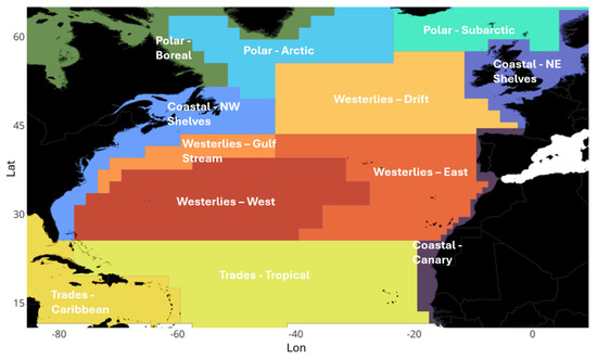
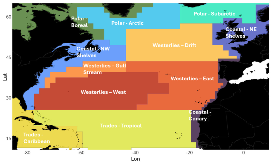
The study area is situated in the North Atlantic Basin, in a region defined by the area ranging from 10°N to 60°N and from 90°W to 10°E. In this study, the synoptic scale of weather and climate patterns was considered, as defined by the WMO, encompassing atmospheric systems with horizontal scales of O (103 km) and temporal scales of several days to weeks [40,41]. To facilitate the analysis, the biogeochemical Longhurst [42] provinces were used to summarise results within the study area (Figure 1 and Supplementary Materials Table S1). These provinces are conceptual divisions of the global ocean, each characterised by distinctive environmental conditions based on the SST, sea surface salinity and chlorophyll concentration, making them suitable to examine the MHW patterns within these different regions and compare them.
Figure 1.
Longhurst provinces in the study area (coloured regions, adapted from [42]).
MHWs were identified according to the Hobday et al. definition [5], with minor modifications. According to this definition, an MHW event occurs when the local temperature exceeds the 90th percentile threshold of the climatology for at least five consecutive days. Additionally, any gap of two days or less between subsequent events is considered part of the same continuous MHW event. To establish a reference climatology, the Hobday definition was modified by calculating both the mean and the 90th percentile of SST over the entire available historical period (1982–2022) for each calendar day, rather than using a fixed 30-year baseline. The reason for this choice was to reduce sensitivity to the selection of a specific 30-year baseline while preserving the original absolute SST values. However, this approach does not remove the influence of the underlying warming trend (for a discussion on the influence of SST trends on MHW detection, see [32,43,44]). Hence, the underlying trend of SST is not totally decoupled from these results, meaning that MHW trends cannot be interpreted solely as changes in the tails of the temperature distribution in the North Atlantic, but also reflect the warming signal of climate change. To reach such a conclusion, one would need to compare shifting climatology baselines and detrending analysis, an effort which was framed as outside of the scope of this study due to its focus on atmospheric drivers. Accordingly, the non-detrended analysis is useful in showing the changes compared to the full period’s mean and 90th percentile. Additionally, a 15-day total running average window was applied, instead of a 30-day window used in Hobday’s definition, in order to reduce excessive inter-weekly smoothing. This methodological choice is motivated by the study’s focus on the atmospheric drivers of MHWs, which typically operate on synoptic to sub-seasonal timescales of approximately 5–20 days [6,12].
Following Hobday’s methodology [5], the resulting MHWs’ daily intensities were then aggregated into annual pixel-wise statistics, including annual frequency (number of events, number of days), mean and maximum intensity, and mean and maximum duration. MHWs spanning two calendar years were assigned to the year in which they ended. This choice may influence annual metrics for long events spanning calendar years, particularly in tropical regions where persistent threshold exceedances occur. Trends in these annual metrics were computed per pixel, using non-parametric statistical methods: the Theil–Sen Slope Estimator and the Mann–Kendall Test [45,46,47,48]. Trend analysis was also conducted per Longhurst province by calculating the spatial averages of the pixel-wise annual metrics.
To investigate the relationship between the occurrence of MHWs and the annual NAO, the composites of the mean annual metrics per positive (NAO > 0, 27 years) and negative (NAO < 0, 14 years) phases were considered. Neutral years were therefore not treated separately; all years were classified by the sign of the annual NAO index. For each NAO phase, composites were constructed by calculating the pixel-wise mean of the annual MHW metrics, resulting in spatial composite fields representing typical MHW conditions during positive and negative NAO years. To evaluate the robustness and statistical significance of the differences of these typical MHW conditions during the two NAO phases, a spatial pattern significance testing framework was applied. This framework involved the computation of several statistical metrics describing both the magnitude and the spatial organisation of the composite field differences across multiple levels of spatial aggregation, i.e., resampling the original pixel size by using a geometric progression with a common ratio (henceforth, k) of 2 (Supplementary Materials Table S2). The spatial aggregation degrades the spatial resolution, reducing small-scale noise and detail, while preserving large-scale spatial structure, enabling assessment of whether the observed differences remain consistent across different physical scales.
Within this framework, the Global Moran’s I statistic [49] was used to test for spatial autocorrelation in the difference of the composite field (NAO+ − NAO−), assessing whether the observed patterns exhibited significant clustering and thus rejecting the null hypothesis of spatial randomness. In addition, the root mean square error (RMSE) and mean absolute deviation (MAD) were calculated to quantify the overall magnitude of the composite differences. To determine the field-level significance associated with the NAO phase, these statistics were further evaluated using a permutation test (based on 999 permutations). Specifically, the NAO sign was randomly reassigned to years, composite differences were recalculated, and the observed statistics were compared against the resulting null distributions. This procedure tested whether the spatial patterns of composite differences could arise by chance. The 999 permutations generated empirical null distributions, representing the expected range of statistic values under the hypothesis that the NAO phase does not influence the spatial patterns. Statistical significance was then assessed by comparing the observed statistics with their respective null distributions using two-sided permutation p-values.
After establishing large-scale spatial significance, the analysis was refined using Local Moran’s I (LISA; [50]) to identify statistically significant local spatial structures over the map of the differences between the two NAO phases composites. These spatial structures were produced using a row-standardised rook-contiguity spatial weights matrix. Each cell was connected to its four orthogonally adjacent neighbours (north, south, east, and west), excluding diagonal neighbours. This method distinguishes High–High (HH; hotspots, high values surrounded by high values) and Low–Low (LL; coldspots, low values surrounded by low values) clusters, as well as High–Low (HL; high values surrounded by low values) and Low–High (LH; low values surrounded by high values) spatial outliers. This step allowed localisation of the regions contributing most strongly to the NAO-related composite differences, without implying causality between the NAO phase and the resulting MHW patterns.
The interannual variability in the expression of the NAO-related spatial signal was assessed by quantifying the similarity between individual annual MHW fields and the respective NAO composite pattern. It should be noted that directly comparing raw yearly maps to the NAO composite patterns leads to high-magnitude years (late years, extreme years) appearing more “similar” because of the larger absolute metric values in recent years, over the whole domain (i.e., due to the underlying trend). To overcome this constraint, the similarity analysis was conducted on z-scored maps (computed as the difference between each cell value and the global mean weighted by latitude divided by the global standard deviation). This ensured that subsequent analyses reflected similarity in spatial organisation rather than absolute intensity. For each year, a spatial pattern correlation was calculated between the MHW fields and the respective NAO composite pattern, yielding a measure of NAO-like spatial pattern expression independent of overall magnitude. These correlation values were subsequently converted to ranks to facilitate robust interannual comparisons and reduce sensitivity to outliers. Temporal autocorrelation was not considered in the NAO-phase permutation procedure because the annual NAO index did not exhibit significant autocorrelation. However, autocorrelation in annual MHW metrics was not explicitly corrected in the trend analysis.
To illustrate NAO-related MHW spatial patterns on MHWs, two case studies were selected, focusing on MHWs that occurred in different years and NAO phases. The first chosen MHW occurred between March and July 2018 within the Westerlies–West region, while the second MHW occurred between November 2009 and October 2010. These two events were chosen for their significant intensity and duration, as well as for the NAO, which was mainly positive in the first event and negative in the second. In addition to the NAO analysis, individual atmospheric fields were incorporated to address their individual contribution to the establishment of that MHW. To do so, the cumulative intensity time series were compared to the mean sea level pressure anomaly, as well as the anomalies of geopotential height, 2 m temperature, latent heat flux, sensible heat flux, longwave radiation, shortwave radiation, net radiative flux (i.e., sum of net shortwave and net longwave radiation), net heat flux and 10 m wind speed. These anomalies were calculated relative to the 1982–2022 daily climatology. It is important to note that the ECMWF convention for vertical fluxes is positive downwards [33]. Following the ECMWF convention used here, positive downward flux anomalies represent anomalous energy gain by the surface, while reduced upward turbulent/radiative losses correspond to anomalous ocean heat retention. Likewise, downwards shortwave and longwave radiation fluxes showing positive anomalies mean that there is more energy than usual being transferred from the atmosphere to the ocean, i.e., an energy gain to the ocean. For the event that occurred in 2018, the daily evolution of the MHW was also considered.
3. Results
3.1. MHW Temporal Evolution and Trends
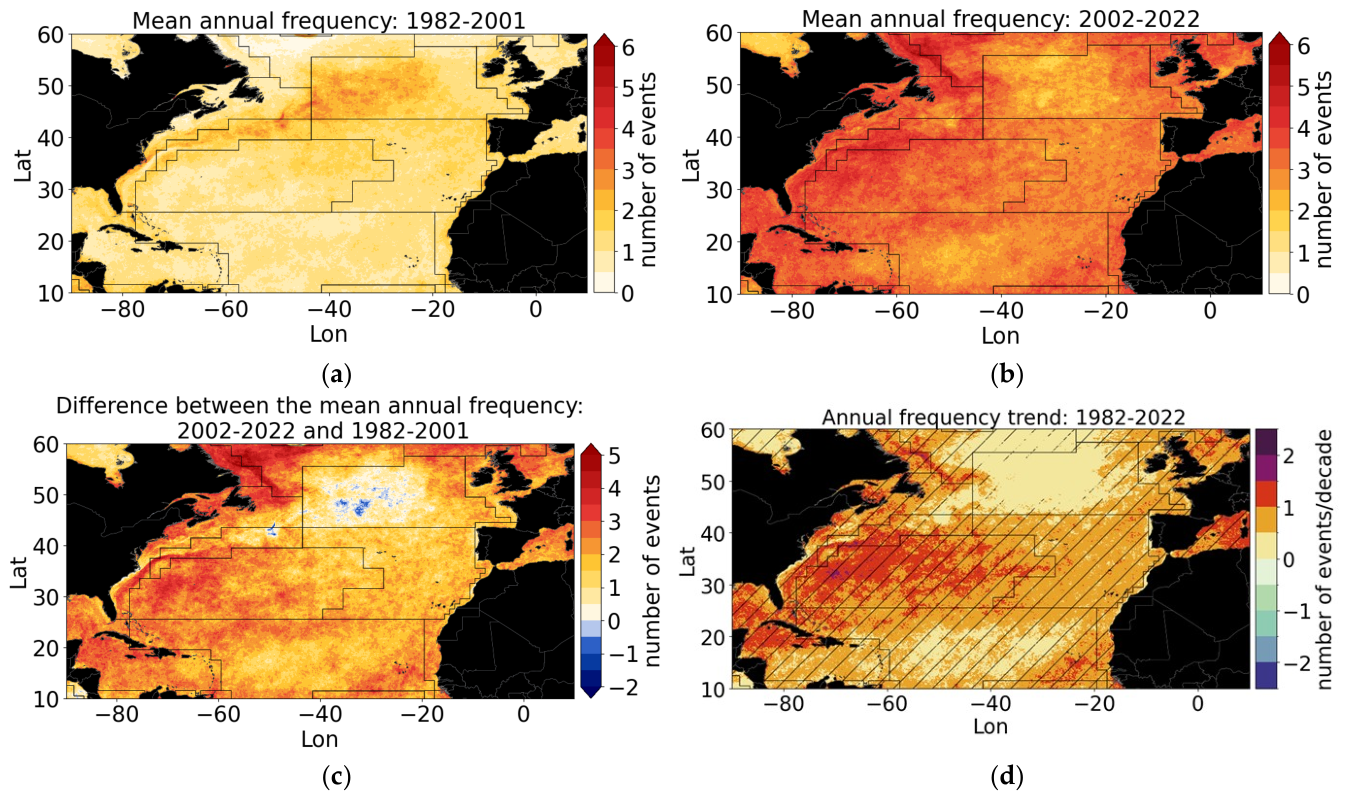
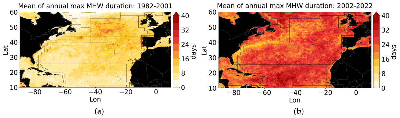
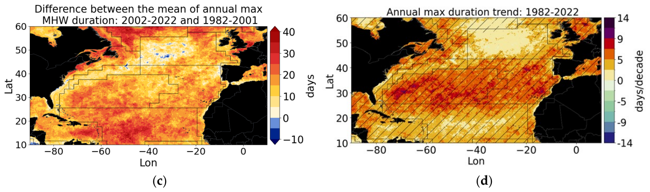
From the 41 years of MHW data, there are distinguishable temporal patterns showing an increasing trend of the MHW annual metrics (frequency of events, maximum duration and maximum intensity), with the results differing between different provinces. Figure 2, Figure 3 and Figure 4 illustrate the spatial patterns of these MHW metrics over the 1982–2001 and 2002–2022 periods, as well as the difference between the two periods. The overall trends (annual mean duration and mean intensity) can be found in Supplementary Materials Figures S1 and S2.
Figure 2.
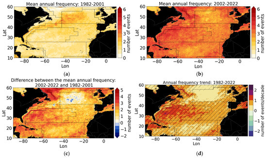
Annual number of MHW events: (a) mean between 1982 and 2001, (b) mean between 2002 and 2022, (c) difference between the two periods, (d) trend between 1982 and 2022. The diagonal lines indicate areas where the trends are statistically significant (p-value < 0.05). Overlayed polygons represent the Longhurst provinces.
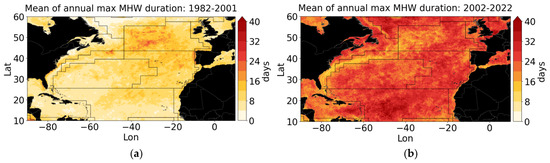
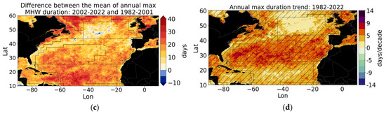
Figure 3.
Annual maximum duration of MHW events: (a) mean between 1982 and 2001, (b) mean between 2002 and 2022, (c) difference between the two periods, (d) trend between 1982 and 2022. The diagonal lines indicate areas where the trends are statistically significant (p-value < 0.05). Overlayed polygons represent the Longhurst provinces.
Figure 4.
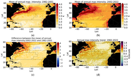
Annual maximum intensity of MHW events: (a) mean between 1982 and 2001, (b) mean between 2002 and 2022, (c) difference between the two periods, (d) trend between 1982 and 2022. The diagonal lines indicate areas where the trends are statistically significant (p-value < 0.05). Overlayed polygons represent the Longhurst provinces.
Agreeing with the warming trends observed in the SST over the North Atlantic basin, positive differences are found in all MHW annual metrics. During the earlier period (1982–2001), the mid-latitude North Atlantic experienced an average of 1.5 MHW events per year, which increased to 3.5 events in the latter period (2002–2022). A particular finding is the contrast among frequency, duration and intensity patterns of change. Frequency and duration reveal the greatest climatology differences in the Westerlies midlatitude regions, with a visible agreement between both maps (Figure 2, Figure 3 and Figure 4c), showing that MHW frequencies have increased by 1 to 2 additional events per year and MHW maximum durations varied by 15 to 20 days per year between the two 20-year periods. In contrast, maximum intensity maps depict an overall much more homogeneous variation (Figure 4), with an average of 1 K of increasing MHW magnitude in almost all the North Atlantic (except in the Gulf Stream). This spatial homogeneity is particularly in agreement with overall global ocean warming trends, which suggests the predominance of an underlying shift in the SST towards greater mean values, rather than increased variation or asymmetry in the upper tails of its distribution.
Regarding the MHW annual metrics trends (Figures S1 and S2), an overall increasing pattern is evident, although not uniformly across the different provinces. The highest trends are generally observed in the mid-latitudes, especially in the Westerlies—East, West and Gulf Stream provinces and also in the Coastal and Polar provinces associated with the North American coast, possibly associated with the Gulf Stream and Labrador Current, with increases of about 0.5 to 2 events/decade, 5 to 9 days/decade in maximum duration and over 0.2 K/decade of maximum intensity. In contrast, there is an overall maintenance in the Westerlies—Drift and Polar—Arctic provinces, potentially associated with the NAWH (also known as the Cold Blob), whereas in the central area of the Drift province, there is even a very small decrease, although not statistically significant in all the annual metrics. Comparing the mean and maximum metrics of MHW duration and intensity trends, it is noticeable that the highest trends are found in the latter, meaning that the fastest change is occurring in the most severe situations.
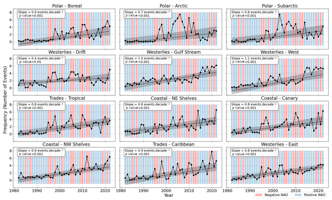
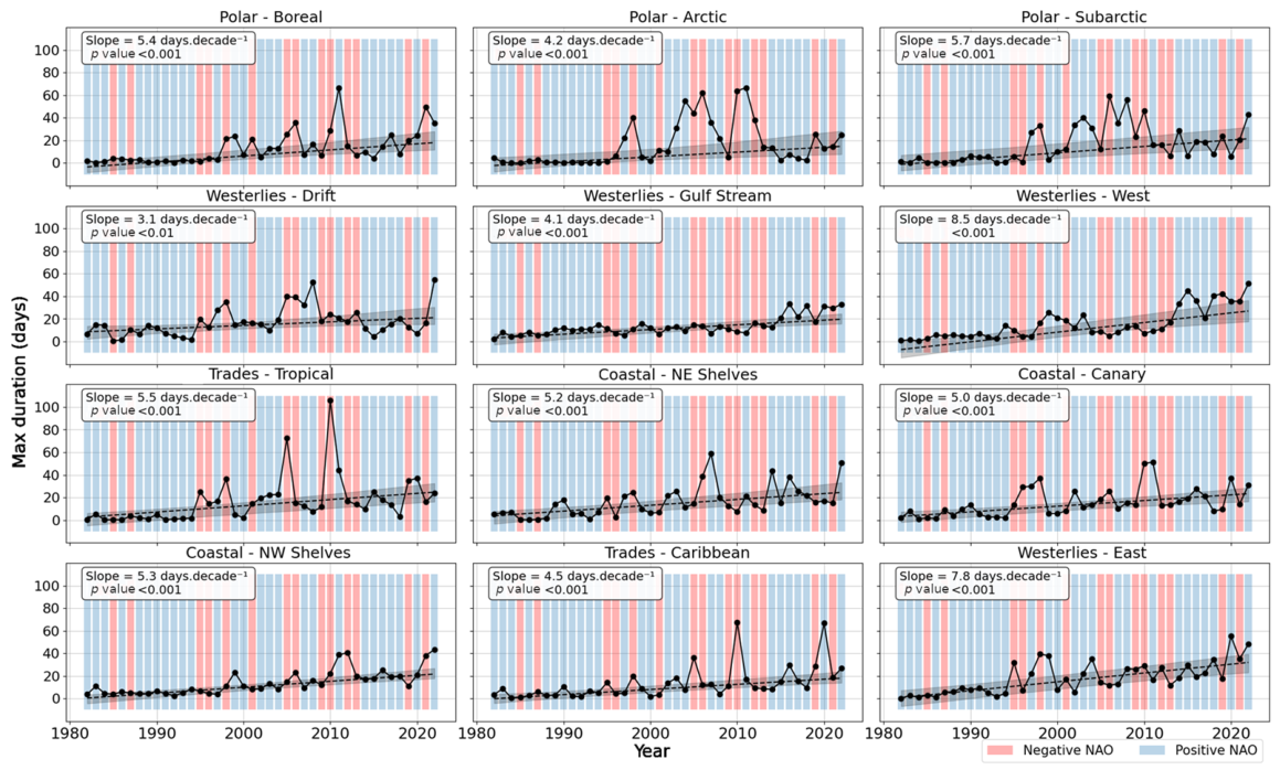
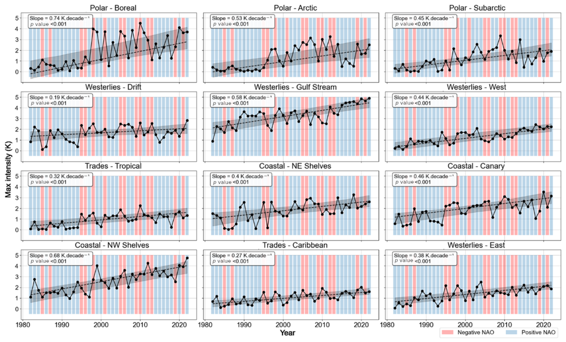
Figure 5, Figure 6 and Figure 7 (and Supplementary Materials Figures S3 and S4) show the time series of MHW annual metrics, averaged per Longhurst provinces, along with their trends and the corresponding annual NAO variability index, represented by the blue and red bars underlying the MHWs metrics time series. These plots reveal increasing trends across most provinces and metrics; however, the apparent acceleration after the mid-1990s is based on visual inspection and should be interpreted cautiously.
Figure 5.
Annual mean frequency (number of events) in each Longhurst province and the corresponding trend. The grey-shaded area represents the uncertainty of the trend line. Blue bars denote years with a positive North Atlantic Oscillation (NAO) index, while red bars denote years with a negative NAO index.
Figure 6.
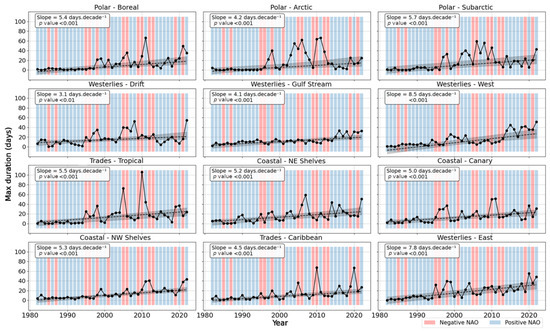
Annual mean of maximum duration in each Longhurst province and the corresponding trend. The grey-shaded area represents the uncertainty of the trend line. Blue bars denote years with a positive North Atlantic Oscillation (NAO) index, while red bars denote years with a negative NAO index.
Figure 7.
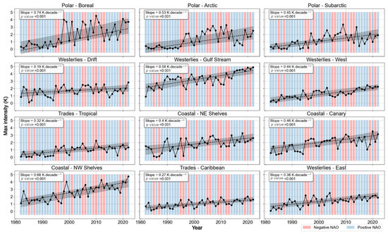
Annual mean of maximum intensity in each Longhurst province and the corresponding trend. The grey-shaded area represents the uncertainty of the trend line. Blue bars denote years with a positive North Atlantic Oscillation (NAO) index, while red bars denote years with a negative NAO index.
A visual inspection suggests that the relationship between MHW annual metrics and the NAO index varies across Longhurst provinces—some show modulation under positive NAO, some under negative NAO, while others show little to no clear NAO influence. The Polar provinces exhibit some of the most pronounced trends in MHW metrics, with maximum intensity showing the strongest increase, rising at a rate of 0.7 K/decade. The annual MHW metrics in these provinces show the most pronounced differences between positive and negative NAO years, with the highest values occurring preferentially during the negative NAO years (less pronounced differences are found in the Polar–Subarctic province). Conversely, in the Westerlies mid-latitude provinces, the MHW metrics show different behaviours according to the longitude as a function of the NAO phase. In the eastern Westerlies–Drift province, the highest metrics are associated with the negative NAO phase. As expected, associated with the influence of the downwelling arm of the North Atlantic general circulation, this province exhibits the lowest trends across all MHW metrics, including the number of events (0.4 events/decade), mean and maximum duration (1.5 and 3.1 days/decade, respectively), mean and maximum intensity (0.03 and 0.2 K/decade, respectively). In contrast, in the Westerlies–West, the highest number of events occur preferentially during the positive NAO phase, which suggests the influence of the Azores high-pressure system on MHW onset. In this province, the number of events and maximum durations show the highest increasing trends, with 1.1 events/decade and 8.5 days/decade, respectively (Figure 5 and Figure 7). In the Westerlies–East, there are no evident differences between the NAO phases. Nonetheless, all overall mean annual MHW metrics are higher during the negative NAO phase. In the Westerlies–Gulf Stream, the difference between MHW metrics for NAO phases is not evident in the time series plots. This province exhibits the highest increasing trend in mean intensity, with a trend of 0.1 K/decade and one of the lowest durations and increases in duration.
3.2. MHW Statistics per NAO Phase
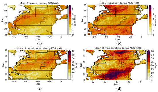
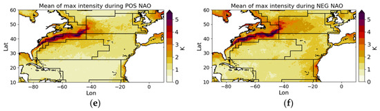
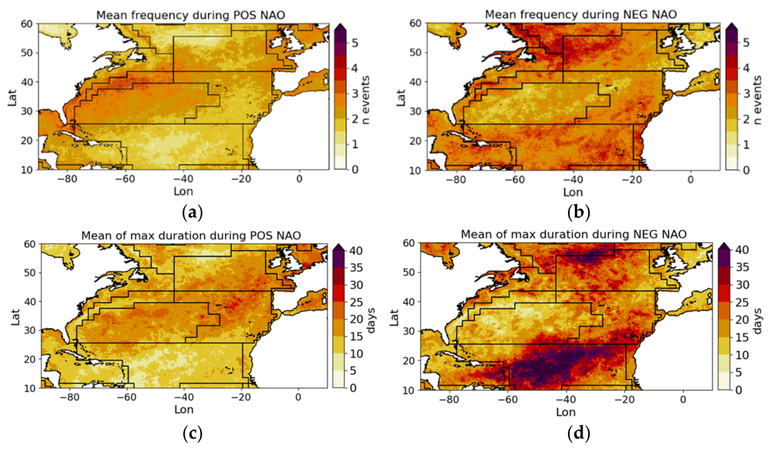
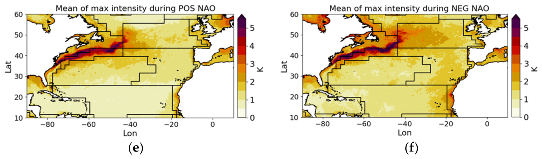
To further clarify the relationship between MHW patterns and the NAO climate mode, Figure 8 presents composites of the MHW metrics, such as the maximum intensity, frequency and duration, per NAO phase. Here, the annual NAO index was considered in order to identify the broad-scale relationship between the NAO phases and MHW characteristics at the basin scale. Knowing that the atmospheric and oceanic conditions prior to the events can influence their occurrence, the annual index provides a representation of the prevailing climate state that may precondition the ocean for MHW development, as well as a representation of the climate state during the events, making it suitable for this analysis. The same analysis was performed for the mean MHW metrics, and the results are presented in Supplementary Materials Figure S5.
Figure 8.
Mean MHW properties for composites of positive (left, 27 years) and negative NAO (right, 14 years) years: (a,b) frequency (number of events), (c,d) maximum duration and (e,f) maximum intensity. Overlayed polygons represent the Longhurst provinces.
The results align with the previous section, presenting a clearer picture of the spatial patterns of MHW prevalence. Additionally, it is evident that the composites of MHW frequency and duration from the positive and negative NAO phases are actually inverse to each other, suggesting that it is possible to identify probabilistic differences between the provinces, although the MHW maximum intensities are shown to be less contrasting. In particular, during the positive NAO phase, the mid-latitude regions of the North Atlantic, such as the Westerlies–West and Gulf Stream provinces and also Coastal–NE Shelves, exhibit higher values for all MHW metrics. This means that the highest frequencies, durations and intensities are associated with this NAO phase in these provinces. Although in the Westerlies–Drift and Westerlies–East provinces, the highest MHW metrics were found in the negative NAO years, significant values in the positive NAO phase were also observed.
These results are generally consistent with the expected atmospheric dynamics, as the positive NAO mode is characterised by a stronger contrast between high- and low-pressure systems, with more persistent and intensified high-pressure systems over the midlatitudes, dominated by the well-known Azores anticyclone. This stability enhances clear-sky conditions, allowing more solar radiation to reach the ocean surface, contributing to surface ocean warming and consequently to higher MHW occurrences, durations and intensities over the mid-latitude provinces. By contrast, during the negative NAO phase, weaker and less stable high- and low-pressure systems result in a diminished atmospheric pressure gradient and stronger surface winds, likely enhancing wind-driven ocean mixing and limiting surface heat accumulation in the mid-latitudes. Under negative NAO conditions, the redistribution of pressure, wind, cloudiness, and heat-flux anomalies may favour MHW development in some polar and tropical sectors, although the mechanism is likely seasonally dependent and may involve both atmospheric and oceanic preconditioning.
Regarding the spatial significance testing, the analysis reveals structurally organised composites of the MHW metrics per NAO phase, with important interannual manifestation. Table 1 (and Supplementary Materials Table S3) shows that the NAO-conditioned composite difference fields exhibit strong spatial clustering across aggregation scales, from native resolution (0.05°, approximately 5.5 km) towards basin-scale smoothing (3.20°, approximately 356 km). This is evident by consistently high Global Moran’s I values (>0.90), indicating a pronounced spatial organisation of the NAO composite differences across resolutions and, consequently, indicating pronounced large-scale spatial coherence in the NAO-conditioned composite differences. The permutation-based fields significance test further confirms that this spatial organisation is significantly stronger than expected under random NAO phase assignment, particularly at mesoscale to regional aggregation levels (k ≈ 2–16). In contrast, magnitude-based metrics (RMSE and MAD) are only marginally significant and depend on the aggregation level, suggesting that the NAO signal is expressed more robustly in the spatial structure of the fields than in their absolute amplitude. In other words, this suggests that the NAO-associated signal is expressed mainly in the spatial organisation of MHW metrics (latitudinal and meridional gradients) rather than in how strong they are.
Table 1.
Statistics and p-values calculated with a permutation test for aggregation level 8 and 16 (~0.4 and 0.8°, corresponding to the regional mesoscale and large regional scales).
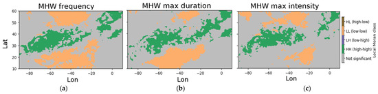
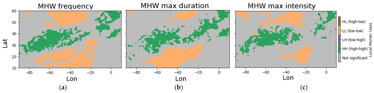
The spatial organisation of the NAO+ − NAO− difference field is significantly stronger than expected by chance, as evidenced by the permutation test on Global Moran’s I. These results reveal a highly coherent spatial organisation across scales (Figure 9 and Supplementary Materials Figure S6). Particularly, the results demonstrate that, among statistically significant locations, more than 99.9% belong to either High–High (associated to the positive NAO composite) or Low–Low (associated with the negative NAO composite) clusters, while spatial outliers (i.e., HL/LH) are negligible, indicating that NAO-related differences arise mostly due to large, coherent spatial regions rather than isolated anomalies. Furthermore, the persistence across scales indicates that the NAO effects are primarily structural rather than localised. In contrast, the overall magnitude of differences (RMSE and MAD) is suggestive but not statistically significant in all MHW metrics, if considering a conventional 0.05 confidence level.
Figure 9.
Local Moran’s I (LISA) cluster maps for NAO-conditioned composite differences in (a) MHW frequency, (b) MHW max duration and (c) MHW max intensity. Results are shown at an aggregation scale of k = 8. HH (High–High) hotspots, high values surrounded by high values, -LL (Low–Low) coldspots, low values surrounded by low values clusters, HL (High–Low) high values surrounded by low values, LH (Low–High) low values surrounded by high values.
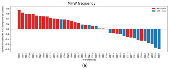
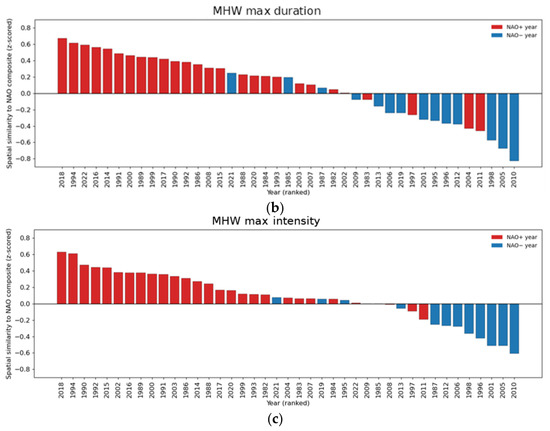
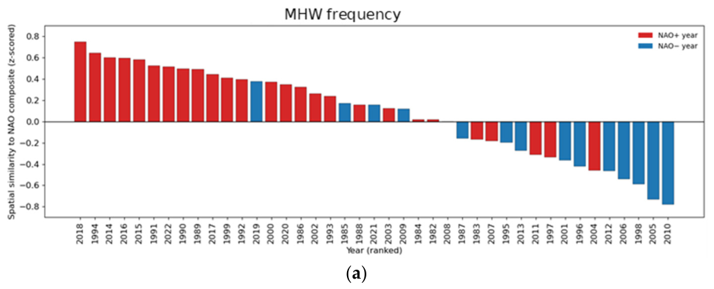
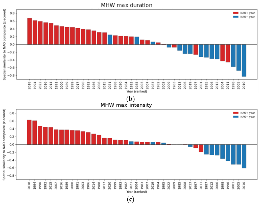
Figure 10 (and Supplementary Materials Figures S7–S11) shows how similar an individual year is to the multi-year positive/negative NAO composite patterns. An aggregation scale of k = 8 was used as the reference scale, as it provides a balance between pattern significance and spatial consistency. Here, the target pattern corresponds to the positive-NAO composite field after z-score standardisation, which means that similarity correlations with a strong positive value correspond to canonical positive NAO years, in that the MHWs metrics spatial patterns closely resemble those of the corresponding composite. Contrariwise, strong negative values indicate significantly dissimilar patterns, as is the case in most of the negative NAO years. Spatial correlation values above 0.75 (below −0.75) are deemed strong indicators of similarity (dissimilarity). Year-to-year pattern similarity analysis reveals substantial interannual variability, with strong alignment to the NAO composite occurring in only a subset of years. This indicates that the NAO-related MHW spatial patterns emerge episodically rather than being persistently expressed. Additionally, pattern similarity remains relatively stable across spatial scales, despite an orders-of-magnitude reduction in the number of significant spatial units at coarser resolutions (Supplementary Materials Table S4).
Figure 10.
Spatial similarity to the NAO composite considering each annual MHW (a) frequency, (b) maximum duration and (c) maximum intensity.
3.3. Case Study Events
3.3.1. Event During Positive NAO: March to July 2018
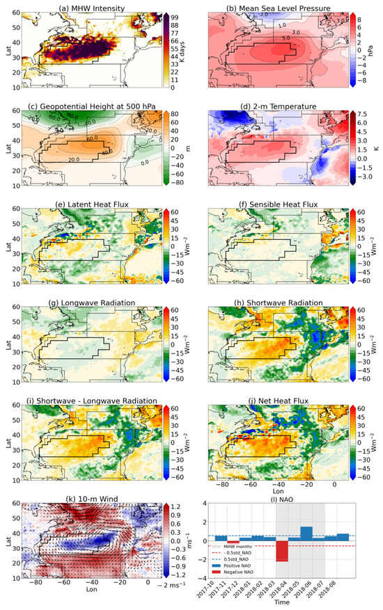
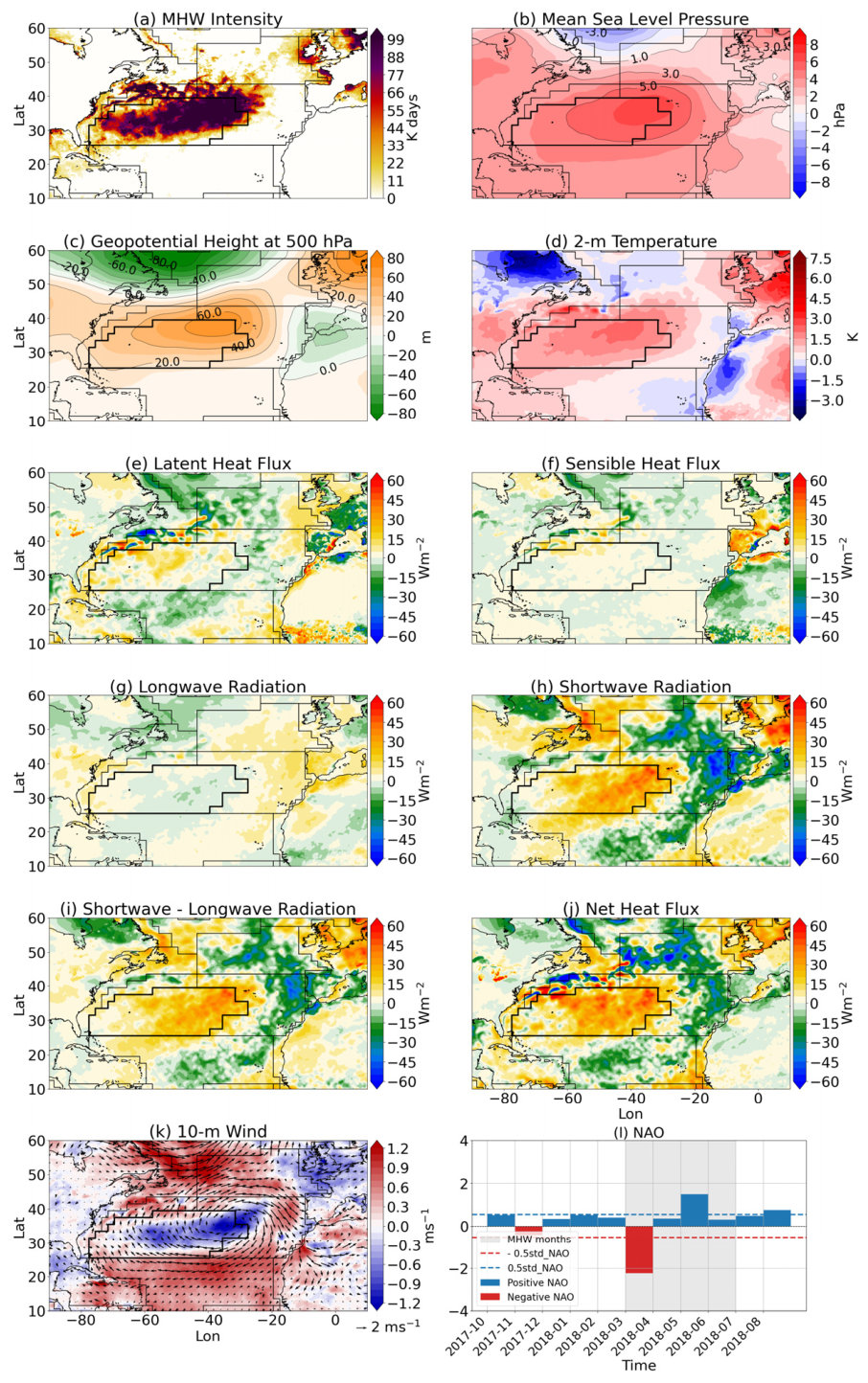
This section presents the analysis of the MHW, which occurred from 21 March 2018 to 7 July 2018, mainly within the Westerlies–West province, lasting 108 days. The selection of this year was based on the visual inspection of the time series maps, from which a significant positive NAO-like canonical pattern seems to emerge. Significantly, this is also supported by the similarity ranking, as the 2018 event is placed in the first place, as the event with the strongest correlation with the positive NAO pattern. Figure 11 shows the cumulative MHW intensity, the mean anomaly of the atmospheric fields over the MHW event period, and the monthly NAO index for the five months preceding the event, during the event and the two months after the event.
Figure 11.
Spatial distribution of the cumulative MHW intensity, atmospheric variables average anomalies over the period from 21 March 2018 until 7 July 2018 and monthly NAO: cumulative MHW intensity, mean sea level pressure, geopotential height, 2 m air temperature, latent heat flux, sensible heat flux, net longwave radiation, net shortwave radiation, net radiative flux (defined as the sum of net shortwave and net longwave radiation), net heat flux, 10 m wind field and wind speed and monthly NAO index (bars represent the NAO monthly value, red dashed line represents 0.5 × standard deviation, blue dashed line represents −0.5 × standard deviation and the shaded grey area represents the months in which the MHW occurs). Overlayed polygons represent the Longhurst provinces.
A spatiotemporal correspondence between the atmospheric anomalies and the MHW intensity patterns suggests a likely relationship between them. The mean sea level pressure and geopotential height anomaly show the presence of a persistent high-pressure system over the MHW area. These atmospheric patterns are expected during the positive NAO phase. The 2 m temperature anomaly also supports this association, with the highest values occurring over the MHW area, while the remaining areas of the North Atlantic basin are experiencing either a negative or positive anomaly, but these are close to zero (except in the Coastal—NE Shelves, where another MHW is occurring). Similarly, there is also a correspondence between the spatial patterns of the heat flux anomalies and the cumulative intensity. Positive sensible and latent heat-flux anomalies in the MHW area indicate reduced turbulent heat loss from the ocean to the atmosphere under the adopted ERA5 sign convention. Increased incoming solar radiation is instead indicated by the positive shortwave-radiation anomaly. The positive anomaly of shortwave radiation indicates increased solar radiation reaching the surface of the ocean in the MHW region, suggesting that it has an important role in the ocean heat budget at that location. These results are confirmed when the combined heat flux anomalies result in a positive net heat flux anomaly, indicating an overall energy gain to the surface of the ocean, while the negative wind speed anomalies over the MHW area suggest lower-than-average ocean surface mixing, consistent with the expected influence of a high-pressure system (see clockwise wind speed vector field). All these factors likely resulted in increased heat gains and reduced ocean vertical mixing, with less energy loss, allowing the SST heating pattern to persist.
The NAO monthly index during the event (Figure 11) is consistent with the previous results, with the event being associated with the positive NAO phase. In the three months before the beginning of the event, the persistence of a positive phase (albeit with weak values) suggests that the NAO is consistent with large-scale atmospheric conditions that may have favoured warming of the surface of the ocean. Despite a strongly negative NAO in April (typically linked to a lower persistence of MHWs in the Westerlies–West province) when the MHW was already established, the ocean surface was possibly already in a warmed state, and the change of the NAO phase was not sufficient to dissipate the MHW. After that, the NAO assumed a positive phase, favourable for MHW persistence. Nevertheless, while the NAO index may provide useful contextual information for MHW occurrence in that province, the index does not explicitly explain the MHW dissipation, since until the end of the MHW, the NAO index remains in a positive phase, suggesting that other processes were more relevant to the MHW offset.
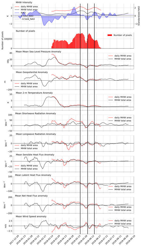
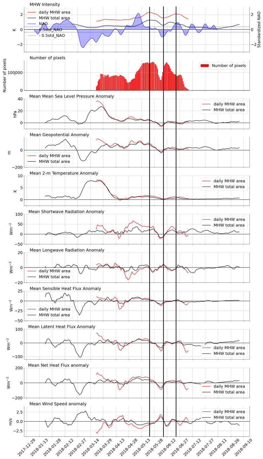
Figure 12 presents the daily evolution of the MHW intensity and extension and atmospheric parameters, which are important to characterise the MHW evolution, along with the daily NAO index. These parameters were averaged for the MHW area on a daily basis (red curve) and for the total area occupied by the MHW (black curve, the period before and after the event was also included).
Figure 12.
Time series of MHW intensities and atmospheric variable anomalies averaged over the daily area of the MHW (red curve) and the total area occupied by the MHW (black curve): mean MHW intensity and standardised NAO (blue curve), MHW extension given by the number of pixels occupied by the MHW, mean sea level pressure, geopotential height, 2 m temperature, net shortwave radiation, net longwave radiation, sensible heat flux, latent heat flux, net heat flux and wind speed. Black vertical lines indicate the two maxima and the minimum of MHW intensity.
In general, a correspondence between the intensity evolution and the atmospheric variables is depicted. The increases in MHW intensity and spatial extent primarily occurred in periods of positive anomalies of mean sea level pressure and geopotential height (and negative anomalies of wind speeds), generally associated with high-pressure systems with weak pressure gradients. These conditions were accompanied by higher-than-usual shortwave radiation, as well as sensible, latent and net heat fluxes, corresponding to an energy gain to the ocean. On the other hand, decreases in MHW intensity and spatial extent occurred typically during periods of negative mean sea level pressure/geopotential height anomalies (potentially with the presence of low-pressure systems or in the transition zone between high- and low-pressure systems), linked to strong pressure gradients and stronger-than-usual wind speeds. Consequently, these conditions were also associated with lower-than-usual shortwave radiation, sensible, latent and net heat fluxes, corresponding to energy gain to the atmosphere. Air temperature anomalies exhibited similar patterns as the mean sea level pressure and geopotential height anomalies, with areas of positive anomalies of these fields corresponding to positive temperature anomaly values (with some associated lag in time). Despite the more effective relationship between daily NAO variations and atmospheric anomaly patterns, the link with MHW intensity evolution is not clear (Figure 12). These relationships are interpreted as physically consistent associations rather than formal attribution, since no lagged correlation, regression, or mixed-layer heat-budget analysis was performed.
3.3.2. Event During Negative NAO: November 2009 to October 2010
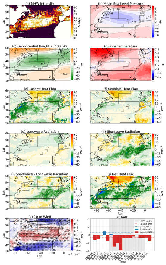
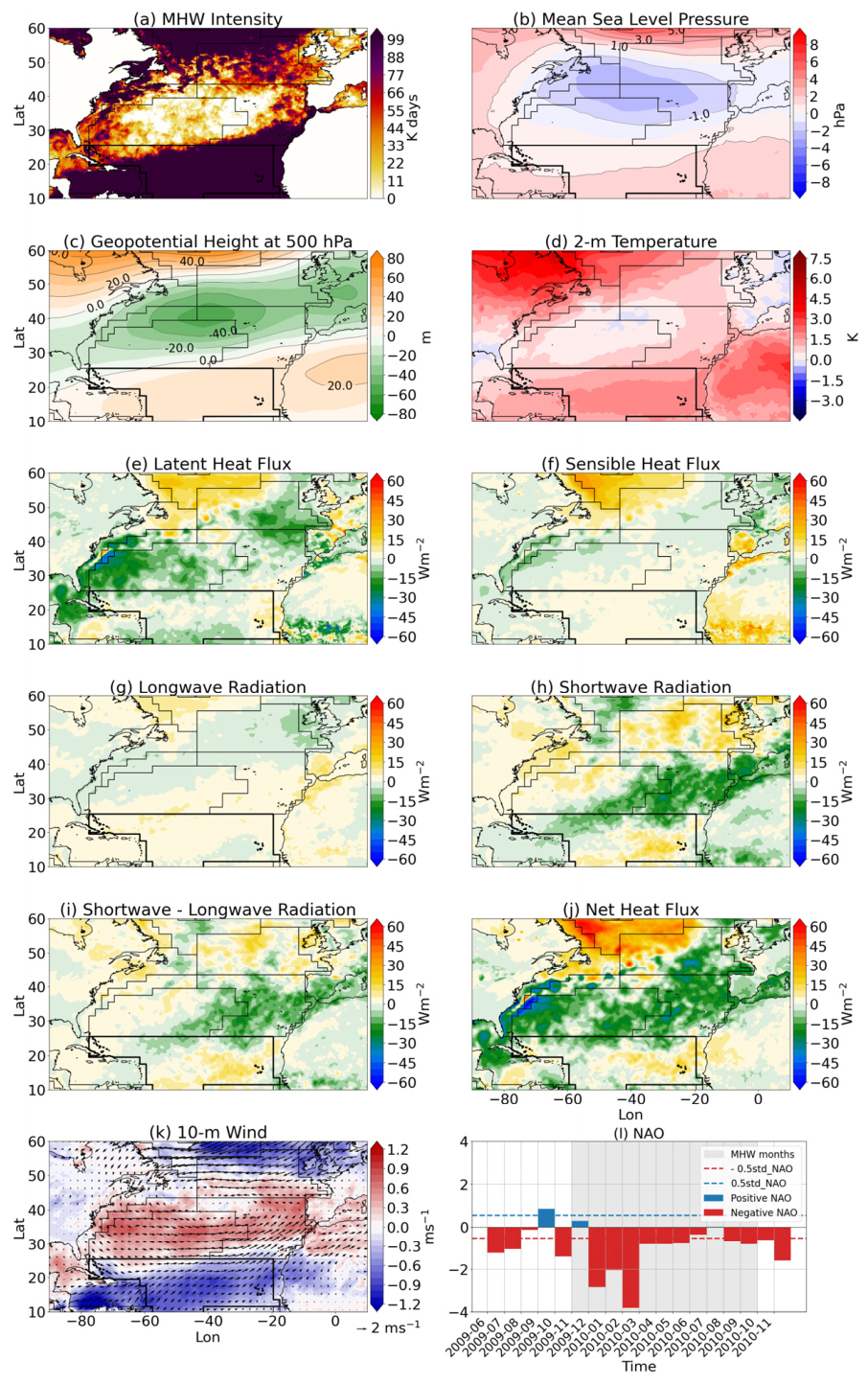
As in the previous section, the selection of this year was based on the visual inspection of the time series maps, from which a negative NAO-like canonical pattern appears to emerge. Again, this is also supported by the similarity ranking, as the 2010 event is placed in last place, as the event with the strongest negative correlation with the positive NAO pattern. The event lasted from 19 November 2009 until 16 October 2010, a total of 331 days, and had a cumulative intensity of about 116 K. During this period, nearly the entire North Atlantic experienced MHW conditions, except for a strip encompassing the Westerlies–West and East provinces. However, here it is important to note that such a long event, and especially in the tropical region where SST variability is relatively low, may reflect the persistent basin-scale warming relative to the climatological period (1982–2022) rather than a discrete MHW event. Nevertheless, it is still interesting to evaluate the atmospheric conditions during this period and to relate them to the MHW conditions.
The event (Figure 13) occurred predominantly during negative NAO months, the most likely situation for the Trades–Tropical province. Accordingly, positive anomalies of sea level pressure and geopotential height prevailed in the tropical latitudes, likely contributing to the formation and maintenance of the MHW through suppressed wind speeds and enhanced solar radiation. In contrast, the regions without MHW conditions were influenced by a mid-latitude low-pressure system, which likely induced unstable atmospheric conditions, with higher-than-average wind speeds, and reduced surface solar radiation, thus contributing to the decrease of heat gains, enabling vertical mixing and potentially preventing the formation of necessary conditions for MHW development.
Figure 13.
Spatial distribution of the cumulative MHW intensity, atmospheric variable average anomalies over the period from 19 November 2009 until 16 October 2010 and monthly NAO: cumulative MHW intensity, mean sea level pressure, geopotential height, 2 m air temperature, latent heat flux, sensible heat flux, net longwave radiation, net shortwave radiation, net radiative flux (defined as the sum of net shortwave and net longwave radiation), net heat flux, 10 m wind field and wind speed and monthly NAO index (bars represent the NAO monthly value, red dashed line represents 0.5 × standard deviation, blue dashed line represents −0.5 × standard deviation and the shaded grey area represents the months in which the MHW occurs). Overlayed polygons represent the Longhurst provinces.
4. Discussion
The analysis of the MHW trends reported in this study agrees with the literature [2,17,30], since it reveals an overall increasing trend in all MHW metrics (frequency, mean and maximum duration and intensity) over the North Atlantic basin, especially in the last decades. The results show that the highest trends are found in the maximum metrics rather than in the mean ones, meaning that the fastest warming is occurring specifically in the most severe events. Nevertheless, the trends are not homogeneous across all provinces, showcasing spatial patterns that reflect the typical SST zonal and meridional gradients in this ocean basin. Hence, the highest trends are observed mainly in the Westerlies –East and West, Coastal–NW and NE Shelves. By contrast, no significant trends are found within the Westerlies–Drift province, potentially linked with the NAWH and its associated negative SST trends [51]. Previous studies attribute these persistent cooler conditions to a slowdown of the AMOC, suggesting that without this weakening, the region would likely experience near-permanent MHW conditions [52]. Nonetheless, autocorrelation was not considered during the trend analysis to account for other types of variability that can impact the annual MHW metrics (such as low-frequency ocean variability, AMOC or basin-scale warming), which can potentially result in overly optimistic p-values.
The results indicate that the annual NAO index is associated with significant differences in the spatial distribution of annual MHW frequency, duration, and intensity of MHWs across the North Atlantic, consistent with the findings of Holbrook et al. [6]. Although the annual NAO composites cannot resolve seasonal mechanisms and may blend winter preconditioning, spring onset, summer surface heating and autumn persistence mechanisms, this analysis provides a first approximation to the broad-scale basin relationship. In positive NAO years, more events with higher durations and intensities are found in the Westerlies–West and Gulf Stream and also in Coastal–NE Shelves provinces. During the negative NAO years, the pattern is reversed, leading to a higher number of events with higher durations and intensities in the Trades–Tropical, Westerlies–East and Coastal–Canary provinces. The spatial variability of MHWs can possibly be explained by the atmospheric patterns and resulting ocean-atmosphere interactions associated with the two NAO phases, similar to the mechanisms driving the North Atlantic SST tripole [53,54,55]. During the positive NAO phase, increased atmospheric stability in mid-latitude regions likely favours a higher prevalence of MHWs in these latitudes. In contrast, in the northern provinces, above 50°N, reduced atmospheric stability inhibits MHW formation. In the southern provinces, with the high-pressure system, there is an intensification of the trade winds, possibly preventing the formation of MHWs. Conversely, during the negative NAO phase, weaker high- and low-pressure systems lead to reduced atmospheric stability in the mid-latitudes, allowing more low-pressure systems to pass over these regions, likely driving reduced heat gains and increased wind-driven ocean mixing, and thus, suppressing MHW formation. On the other hand, in northern latitudes, reduced wind speeds possibly create more favourable conditions for MHW formation than usual.
Permutation tests based on random reassignment of NAO phases demonstrate that the spatial organisation of NAO-conditioned MHW differences is significantly stronger than expected under the null hypothesis at mesoscale to regional aggregation levels (k = 2–16; two-sided p ≤ 0.05). In contrast, differences in overall magnitude, assessed using RMSE and MAD, are marginally significant (p ≈ 0.08), indicating that NAO should be associated with differences in the spatial distribution of MHW occurrences, intensity and duration rather than inducing uniform changes in event characteristics. Year-to-year pattern similarity analysis further reveals that this NAO-related spatial organisation is expressed episodically, with strong alignment occurring in a limited subset of years rather than consistently across all NAO-positive or NAO-negative conditions. The annual NAO index is therefore useful for assessing the relative level of MHW impact across provinces and shows potential for improving probabilistic MHW predictions, although it does not inform about the NAO’s influence over the main MHW metrics (intensity, duration or frequency). Therefore, a more detailed analysis is necessary to highlight the role of other climate modes in modulating NAO’s role (for example, the Eastern Atlantic and Scandinavian Patterns) at annual, seasonal or monthly scales. Such analysis will be subject to future work.
Although the relationship between atmospheric drivers and MHW intensities was not quantified, the spatial correspondence between atmospheric anomalies and MHW patterns is consistent with known MHW-favourable mechanisms. This MHW occurred predominantly in areas of positive anomalies of mean sea level pressure and geopotential height, particularly within the areas of the high-pressure systems where pressure gradients are weaker, conditions widely recognised as conducive to MHW development [6,14,17]. Due to very stable atmospheric conditions, lower-than-average wind speeds reduce vertical mixing, allowing the incoming solar energy to be retained on the surface of the ocean and reducing heat loss to the atmosphere in the form of turbulent heat fluxes (sensible and latent heat fluxes) [14]. These results suggest that the 2018 event is consistent with a commonly reported MHW-favourable configuration for MHW occurrence: when the ocean retains more energy than usual, resulting from enhanced shortwave radiation absorption and reduced turbulent heat loss, as well as above-average latent and sensible heat flux contributions. The results suggest a relationship between MHWs, longwave radiation, and 2 m air temperature, although a more detailed analysis is required to fully understand these interactions and the potential ocean–atmosphere feedbacks involved. The analysis was conducted only for 12 UTC. While this time captures daytime synoptic conditions associated with radiative forcing, it limits the interpretation of the daily heat budget.
Despite the strong performance of the proposed methodology in assessing the role of atmospheric variables and the NAO in explaining MHW characteristics across several North Atlantic regions, this study has some limitations. First of all, the Hobday et al. [5] method particularly fails to account for the presence of long-term trends within the SST time series, as it operates under the assumption of SST stationarity by using a fixed climatology. While this is useful for long-term climate anomaly assessment, WMO guidelines [40] recommend the 1991–2020 climatological period for recent climate monitoring; using such a recent baseline may reduce the number of detected MHWs relative to earlier fixed baselines [43]. Indeed, given the substantial increase in SSTs over time due to anthropogenic climate change, especially if focusing on variability, some authors argue that it is preferable to adjust the climatology baseline to reflect current and future conditions [36]. To avoid classifying ongoing elevated temperatures as a permanent state of MHW, one solution is to use a moving climatology [12,43,56]. Nevertheless, looking at impacts, it is still unclear what reference should be and whether a single statistical/climatological one is useful compared to organism-related thermal optimum thresholds [43]. In this study, the use of the 1982–2022 period as the reference climatology represents a limitation, especially as the NAO-related composites may be partially influenced by the chosen MHW definition and the selected climatological baseline.
Another important limitation of this study lies in the way atmospheric drivers were analysed—primarily through their spatial agreement with MHW patterns. While this approach can identify potential associations, it does not allow for conclusions about causality. As a result, the statistical significance of the relationships remains unclear, albeit supported by the known physical mechanisms underlying the observed atmospheric and MHW patterns. Furthermore, it should be noted that MHW atmospheric drivers are much more complex than NAO alone. As discussed in the introduction, there are several other drivers involved in a complex multivariate system where, for example, atmospheric blocking, changes in mixed-layer depth, ocean heat advection or even complementary climate modes (e.g., East Atlantic and Scandinavian patterns) may strongly influence the spatial patterns of MHWs. Therefore, the two MHW events described as canonical examples of positive and negative NAO phases should not be understood as the recurrent and expected situation whenever such a phase occurs. Indeed, what the statistical test shows is that many MHW events are not substantially similar to the composite patterns, therefore indicating that NAO alone is insufficient to explain the mechanisms leading to MHW onset and persistence.
Future research should therefore focus on establishing statistical significance and process-based analyses to better understand the cause-and-effect dynamics between atmospheric variability/atmospheric drivers and MHW development.
5. Conclusions
Climate change is driving changes in the climate system, leading to disruptions in the Earth’s energy balance, changing both oceanic and atmospheric patterns. MHW events are becoming more frequent, intense, and prolonged, highlighting their growing significance as a research priority. Yet, many studies focus on specific regions, while basin-scale analyses of North Atlantic MHW variability and associated atmospheric patterns remain comparatively limited. This study focused on the MHW trends and atmospheric drivers in the North Atlantic between 1982 and 2022, with the following conclusions:
- MHWs have become more frequent, intense and prolonged across almost all the North Atlantic, particularly since 1995, although the trends are not uniform across all provinces. These results are dependent on the choice of the reference climatology period (1982–2022).
- The Westerlies–East and West, Coastal–NW and NE Shelves provinces exhibit the strongest increases in the annual number of events, intensity and duration.
- The Westerlies–Drift shows no significant trends, potentially associated with the NAWH.
- MHWs in the positive and negative NAO phases exhibit different statistically significant spatial distributions, like the spatial patterns of the North Atlantic SST tripole. The Westerlies–West and Gulf Stream and Coastal–NE Shelves provinces experience, on average, the highest frequencies, durations and intensities in the positive NAO phase, unlike the Polar, Westerlies–East and Trades–Tropical provinces, which experience the highest values in the negative NAO phase. The NAO appears to be associated with large-scale organisation of MHW spatial structure, but its imprint on event frequency, maximum duration and maximum intensity is conditional, scale-dependent, and intermittently expressed in time rather than uniformly present across all years of a given NAO phase.
- For the two analysed case studies, MHW’s spatial extent and intensity show correspondence with positive mean sea-level pressure, geopotential height, 2 m air temperature, net heat flux, and shortwave-radiation anomalies, as well as with weak pressure gradients and negative wind-speed anomalies.
To conclude, in the context of ongoing climate change, the results presented in this study underscore the importance of MHWs as key indicators of ocean warming. Understanding their trends and atmospheric drivers at the scale of an entire ocean basin is therefore essential for anticipating future risks, improving climate projections, and informing adaptation strategies in a progressively warmer world.
Supplementary Materials
The following supporting information can be downloaded at https://www.mdpi.com/article/10.3390/rs18142363/s1, Figure S1. Annual mean duration of MHW events: (a) mean between 1982 and 2001, (b) mean between 2002 and 2022, (c) difference between the two periods, (d) trend between 1982 and 2022. The diagonal lines indicate areas where the trends are statistically significant (p-value < 0.05). Figure S2. Annual mean intensity of MHW events: (a) mean between 1982 and 2001, (b) mean between 2002 and 2022, (c) difference between the two periods, (d) trend between 1982 and 2022. The diagonal lines indicate areas where the trends are statistically significant (p-value < 0.05). Figure S3. Annual mean MHW duration in each Longhurst province and the corresponding trend. The black-shaded area represents the uncertainty of the trend line. Blue bars denote years with a positive North Atlantic Oscillation (NAO) index, while red bars denote years with a negative NAO index. Figure S4. Annual mean MHW intensity in each Longhurst province and the corresponding trend. The black-shaded area represents the uncertainty of the trend line. Blue bars denote years with a positive North Atlantic Oscillation (NAO) index, while red bars denote years with a negative NAO index. Figure S5. Mean MHW properties for composites of positive and negative NAO years: (a,b) mean duration, (c,d) mean intensity. Figure S6. Local Moran’s I (LISA) cluster maps for NAO-conditioned composite differences in (a) MHW mean duration, (b) MHW mean duration. Results are shown at an aggregation scale of k = 8. Figure S7. Spatial similarity to the NAO composite: (a) mean intensity, (b) mean duration. Figure S8. Spatial similarity to the NAO composite and NAO annual index: (a) frequency, (b) max duration, (c) max intensity, (d) mean duration, (e) mean intensity. Figure S9. Years exhibiting the highest similarity to the NAO composite pattern for the annual frequency metric. Left panels correspond to positive NAO phases, while right panels correspond to negative NAO phases. Figure S10. Years exhibiting the highest similarity to the NAO composite pattern for the annual maximum duration metric. Left panels correspond to positive NAO phases, while right panels correspond to negative NAO phases. Figure S11. Years exhibiting the highest similarity to the NAO composite pattern for the annual maximum intensity metric. Left panels correspond to positive NAO phases, while right panels correspond to negative NAO phases.Table S1. Longhurst provinces modified from [35]. On the left the common name and on the right the short name used in this study. Table S2. Aggregation parameterisation and spatial scale conversion (k is the size of the aggregation window in number of grid cells). Table S3. Moran’s I, RMSE and MAD statistics and p-values calculated with a permutation test for aggregation levels 2 to 32. Table S4. Similarity metrics (correlation) and number of significant cells for different aggregation~levels.
Author Contributions
Conceptualization, B.L., A.O. and C.G.; methodology, B.L., A.O. and C.G.; software, B.L. and J.P.; validation, F.S. and C.G.; formal analysis, B.L.; investigation, B.L.; resources, F.S.; data curation, B.L. and J.P.; writing—original draft preparation, B.L.; writing—review and editing, F.S., A.O. and C.G.; visualization, B.L.; supervision, A.O. and C.G.; project administration, A.O.; funding acquisition, A.O. All authors have read and agreed to the published version of the manuscript.
Funding
This research was funded by Horizon Europe Project ObsSea4Clim: Ocean observations and indicators for climate and assessments (funded by the European Union, Grant Agreement number: 101136548) and supported by the Recovery and Resilience Plan Investment RE-C05-i02: Interface Mission—CoLAB, certified by the National Innovation Agency (Project No. 01/C05-i02/2022).
Data Availability Statement
The datasets used in this study are publicly available. The C3S and ESA CCI SST and ERA5 datasets were obtained from the Copernicus Climate Change platform (SST: https://cds.climate.copernicus.eu/datasets/satellite-sea-surface-temperature?tab=overview, ERA% on pressure levels: https://cds.climate.copernicus.eu/datasets/reanalysis-era5-pressure-levels?tab=overview, ERA5 on single levels: https://cds.climate.copernicus.eu/datasets/reanalysis-era5-single-levels?tab=overview). The NAO annual and monthly data were obtained from NCAR Hurrell NAO Index (PC-based) (https://climatedataguide.ucar.edu/climate-data/hurrell-north-atlantic-oscillation-nao-index-pc-based). The daily NAO index was obtained from NOAA (https://www.cpc.ncep.noaa.gov/products/precip/CWlink/pna/nao.shtml). (All accessed on 17 April 2025). The MHW annual metrics produced in this study are openly available in Zenodo under the DOI 10.5281/zenodo.21361349.
Conflicts of Interest
The authors declare no conflicts of interest.
Abbreviations
The following abbreviations are used in this manuscript:
| AMOC | Atlantic Meridional Overturning Circulation |
| CDR | Climate Data Records |
| CDS | Climate Data Store |
| ECMWF | European Centre for Medium-Range Weather Forecasts |
| ECV | Essential Climate Variable |
| EOF | Empirical Orthogonal Function |
| EOV | Essential Ocean Variable |
| ESA CCI | European Space Agency Climate Change Initiative |
| IPCC | Intergovernmental Panel on Climate Change |
| K | Kelvin |
| MHW | Marine Heatwave |
| NAO | North Atlantic Oscillation |
| NOAA | National Oceanic and Atmospheric Administration |
| NW | Northwest |
| PCA | Principal Component Analysis |
| SST | Sea Surface Temperature |
| WMO | World Meteorological Organization |
References
- Frölicher, T.L.; Fischer, E.M.; Gruber, N. Marine heatwaves under global warming. Nature 2018, 560, 360–364. [Google Scholar] [CrossRef] [Scilit] [PubMed]
- Oliver, E.C.J.; Donat, M.G.; Burrows, M.T.; Moore, P.J.; Smale, D.A.; Alexander, L.V.; Benthuysen, J.A.; Feng, M.; Sen Gupta, A.; Hobday, A.J.; et al. Longer and more frequent marine heatwaves over the past century. Nat. Commun. 2018, 9, 1324. [Google Scholar] [CrossRef] [Scilit] [PubMed]
- Intergovernmental Panel on Climate Change (IPCC). Climate Change 2021: The Physical Science Basis: Contribution of Working Group I to the Sixth Assessment Report of the Intergovernmental Panel on Climate Change; Cambridge University Press: Cambridge, UK, 2023. [Google Scholar] [CrossRef] [Scilit]
- Hobday, A.J.; Oliver, E.C.J.; Sen Gupta, A.; Benthuysen, J.A.; Burrows, M.T.; Donat, M.G.; Holbrook, N.J.; Moore, P.J.; Thomsen, M.S.; Wernberg, T.; et al. Categorizing and naming marine heatwaves. Oceanography 2018, 31, 162–173. [Google Scholar] [CrossRef] [Scilit]
- Hobday, A.J.; Alexander, L.V.; Perkins, S.E.; Smale, D.A.; Straub, S.C.; Oliver, E.C.J.; Benthuysen, J.A.; Burrows, M.T.; Donat, M.G.; Feng, M.; et al. A hierarchical approach to defining marine heatwaves. Prog. Oceanogr. 2016, 141, 227–238. [Google Scholar] [CrossRef] [Scilit]
- Holbrook, N.J.; Scannell, H.A.; Sen Gupta, A.; Benthuysen, J.A.; Feng, M.; Oliver, E.C.J.; Alexander, L.V.; Burrows, M.T.; Donat, M.G.; Hobday, A.J.; et al. A global assessment of marine heatwaves and their drivers. Nat. Commun. 2019, 10, 2624. [Google Scholar] [CrossRef] [Scilit] [PubMed]
- Oliver, E.C.J. Mean warming not variability drives marine heatwave trends. Clim. Dyn. 2019, 53, 1653–1659. [Google Scholar] [CrossRef] [Scilit]
- Plecha, S.M.; Soares, P.M.M. Global marine heatwave events using the new CMIP6 multi-model ensemble: From shortcomings in present climate to future projections. Environ. Res. Lett. 2019, 15, 124058. [Google Scholar] [CrossRef] [Scilit]
- Plecha, S.M.; Soares, P.M.M.; Silva-Fernandes, S.M.; Cabos, W. On the uncertainty of future projections of marine heatwave events in the North Atlantic Ocean. Clim. Dyn. 2021, 56, 2027–2056. [Google Scholar] [CrossRef] [Scilit]
- Smale, D.A.; Wernberg, T.; Oliver, E.C.J.; Thomsen, M.S.; Harvey, B.P.; Straub, S.C.; Burrows, M.T.; Alexander, L.V.; Benthuysen, J.A.; Donat, M.G.; et al. Marine heatwaves threaten global biodiversity and the provision of ecosystem services. Nat. Clim. Change 2019, 9, 306–312. [Google Scholar] [CrossRef] [Scilit]
- Smith, K.E.; Burrows, M.T.; Hobday, A.J.; King, N.G.; Moore, P.J.; Sen Gupta, A.; Thomsen, M.S.; Wernberg, T.; Smale, D.A. Biological impacts of marine heatwaves. Annu. Rev. Mar. Sci. 2023, 15, 119–145. [Google Scholar] [CrossRef] [Scilit] [PubMed]
- Oliver, E.C.J.; Benthuysen, J.A.; Darmaraki, S.; Donat, M.G.; Hobday, A.J.; Holbrook, N.J.; Schlegel, R.W.; Gupta, A.S. Marine heatwaves. Annu. Rev. Mar. Sci. 2021, 13, 313–342. [Google Scholar] [CrossRef] [Scilit] [PubMed]
- Barriopedro, D.; García-Herrera, R.; Ordóñez, C.; Miralles, D.G.; Salcedo-Sanz, S. Heat waves: Physical understanding and scientific challenges. Rev. Geophys. 2023, 61, e2022RG000780. [Google Scholar] [CrossRef] [Scilit]
- Holbrook, N.J.; Sen Gupta, A.; Oliver, E.C.J.; Hobday, A.J.; Benthuysen, J.A.; Scannell, H.A.; Smale, D.A.; Wernberg, T. Keeping pace with marine heatwaves. Nat. Rev. Earth Environ. 2020, 1, 482–493. [Google Scholar] [CrossRef] [Scilit]
- Capotondi, A.; Rodrigues, R.R.; Sen Gupta, A.; Benthuysen, J.A.; Deser, C.; Frölicher, T.L.; Lovenduski, N.S.; Amaya, D.J.; Le Grix, N.; Xu, T.; et al. A global overview of marine heatwaves in a changing climate. Commun. Earth Environ. 2024, 5, 701. [Google Scholar] [CrossRef] [Scilit]
- Sala, J.; Giglio, D.; Capotondi, A.; Sukianto, T.; Kuusela, M. Leading dynamical processes of global marine heatwaves in an ocean state estimate. Ocean Sci. 2025, 21, 2463–2479. [Google Scholar] [CrossRef] [Scilit]
- Sen Gupta, A.; Thomsen, M.; Benthuysen, J.A.; Hobday, A.J.; Oliver, E.; Alexander, L.V.; Burrows, M.T.; Donat, M.G.; Feng, M.; Holbrook, N.J.; et al. Drivers and impacts of the most extreme marine heatwaves events. Sci. Rep. 2020, 10, 19359. [Google Scholar] [CrossRef] [Scilit] [PubMed]
- Schlegel, R.W.; Oliver, E.C.J.; Chen, K. Drivers of marine heatwaves in the Northwest Atlantic: The role of air–sea interaction during onset and decline. Front. Mar. Sci. 2021, 8, 627970. [Google Scholar] [CrossRef] [Scilit]
- Bonino, G.; McAdam, R.; Athanasiadis, P.; Cavicchia, L.; Rodrigues, R.R.; Scoccimarro, E.; Tibaldi, S.; Masina, S. Mediterranean summer marine heatwaves triggered by weaker winds under subtropical ridges. Nat. Geosci. 2025, 18, 848–853. [Google Scholar] [CrossRef] [Scilit]
- Gregory, C.H.; Holbrook, N.J.; Marshall, A.G.; Spillman, C.M. Atmospheric drivers of Tasman Sea marine heatwaves. J. Clim. 2023, 36, 5197–5214. [Google Scholar] [CrossRef] [Scilit]
- Rodrigues, R.R.; Taschetto, A.S.; Sen Gupta, A.; Foltz, G.R.; Dommenget, D.; Marsland, S.J.; McPhaden, M.J. Common Cause for Severe Droughts in South America and Marine Heatwaves in the South Atlantic. Nat. Geosci. 2019, 12, 620–626. [Google Scholar] [CrossRef] [Scilit]
- Niu, X.; Chen, Y.; Le, C. Northeast Pacific marine heatwaves associated with high-latitude atmospheric blocking. Environ. Res. Lett. 2024, 19, 014025. [Google Scholar] [CrossRef] [Scilit]
- Chen, K.; Gawarkiewicz, G.G.; Lentz, S.J.; Bane, J.M. Diagnosing the warming of the Northeastern U.S. coastal ocean in 2012: A linkage between the atmospheric jet stream variability and ocean response. J. Geophys. Res. Oceans 2014, 119, 218–227. [Google Scholar] [CrossRef] [Scilit]
- Chen, K.; Gawarkiewicz, G.; Kwon, Y.O.; Zhang, W.G. The role of atmospheric forcing versus ocean advection during the extreme warming of the Northeast U.S. continental shelf in 2012. J. Geophys. Res. Oceans 2015, 120, 4324–4339. [Google Scholar] [CrossRef] [Scilit]
- Perez, E.; Ryan, S.; Andres, M.; Gawarkiewicz, G.; Ummenhofer, C.C.; Bane, J.; Haines, S. Understanding physical drivers of the 2015/16 marine heatwaves in the Northwest Atlantic. Sci. Rep. 2021, 11, 17623. [Google Scholar] [CrossRef] [Scilit] [PubMed]
- England, M.H.; Li, Z.; Huguenin, M.F.; Kiss, A.E.; Sen Gupta, A.; Holmes, R.M.; Rahmstorf, S. Drivers of the extreme North Atlantic marine heatwave during 2023. Nature 2025, 642, 636–643. [Google Scholar] [CrossRef] [Scilit] [PubMed]
- Global Climate Observing System (GCOS). Implementation Plan for the Global Observing System for Climate (GCOS-244); WMO: Geneva, Switzerland, 2022; Available online: https://library.wmo.int/records/item/58104-the-2022-gcos-implementation-plan-gcos-244?offset=5 (accessed on 17 April 2025).
- Merchant, C.J.; Embury, O.; Bulgin, C.E.; Block, T.; Corlett, G.K.; Fiedler, E.; Good, S.A.; Mittaz, J.; Rayner, N.A.; Berry, D.; et al. Satellite-based time-series of sea-surface temperature since 1981 for climate applications. Sci. Data 2019, 6, 223. [Google Scholar] [CrossRef] [Scilit] [PubMed]
- Copernicus Climate Change Service. Product Quality Assessment Report of Version 2.1 SST Products (v3.0) (PQAR of v2.1SST products v5.1). 2021. Available online: https://dast.copernicus-climate.eu/documents/satellite-ist-sst-global/WP2-FDDP-SST-PQAR-v1.1_Final-2.pdf (accessed on 17 April 2025).
- Santos, R.; Russo, A.; Gouveia, C.M. Co-occurrence of marine and atmospheric heatwaves with drought conditions and fire activity in the Mediterranean region. Sci. Rep. 2024, 14, 19233. [Google Scholar] [CrossRef] [Scilit] [PubMed]
- Bonino, G.; Galimberti, G.; Masina, S.; McAdam, R.; Clementi, E. Machine learning methods to predict sea surface temperature and marine heatwave occurrence: A case study of the Mediterranean Sea. Ocean Sci. 2024, 20, 417–432. [Google Scholar] [CrossRef] [Scilit]
- Hayward, A.; Dasgupta, N.; McAdam, R.; Payne, M.R.; Raj, R.P.; Bonino, G.; Chatterjee, S.; Combes, V.; Denaxa, D.; De Rovere, F.; et al. Marine heat waves—Multiple analysis/definitions (MHW-MAD): A multi-definition global marine heatwave dataset from satellite sea surface temperature data. Earth Syst. Sci. Data Discuss. 2025. preprint. [Google Scholar] [CrossRef] [Scilit]
- Hersbach, H.; Bell, B.; Berrisford, P.; Hirahara, S.; Horányi, A.; Muñoz-Sabater, J.; Nicolas, J.; Peubey, C.; Radu, R.; Schepers, D.; et al. The ERA5 global reanalysis. Q.J.R. Meteorol. Soc. 2020, 146, 1999–2049. [Google Scholar] [CrossRef] [Scilit]
- Paredes-Fortuny, L.; Pastor, F.; Khodayar, S. Concurrent atmospheric heatwaves intensify marine heatwaves through air-sea heat flux change in the Mediterranean Sea. Commun. Earth Environ. 2025, 6, 638. [Google Scholar] [CrossRef] [Scilit]
- National Center for Atmospheric Research (NCAR). Hurrell North Atlantic Oscillation (NAO) Index (PC-Based). 2003. Available online: https://climatedataguide.ucar.edu/climate-data/hurrell-north-atlantic-oscillation-nao-index-pc-based (accessed on 17 April 2025).
- Hurrell, J.W.; Kushnir, Y.; Ottersen, G.; Visbeck, M. An overview of the North Atlantic Oscillation. In The North Atlantic Oscillation: Climate Significance and Environmental Impact; Cambridge University Press: Cambridge, UK, 2024. [Google Scholar]
- National Center for Atmospheric Research (NCAR). Hurrell North Atlantic Oscillation Index (Monthly and Annual Values). 2023. Available online: https://climatedataguide.ucar.edu (accessed on 17 April 2025).
- NOAA Climate Prediction Center. North Atlantic Oscillation (NAO). National Centers for Environmental Prediction, National Weather Service. Available online: https://www.cpc.ncep.noaa.gov/products/precip/CWlink/pna/nao.shtml (accessed on 17 April 2025).
- Barnston, A.G.; Livezey, R.E. Classification, seasonality and persistence of low-frequency atmospheric circulation patterns. Mon. Weather Rev. 1987, 115, 1083–1126. [Google Scholar] [CrossRef]
- World Meteorological Organization. International Meteorological Vocabulary (WMO-No. 182); World Meteorological Organization: Geneva, Switzerland, 2017; Available online: https://library.wmo.int/viewer/35809/ (accessed on 17 April 2025).
- United Nations. Synoptic Scale [Term Entry]. United Nations Multilingual Terminology Database (UNTERM), n.d. Available online: https://unterm.un.org/unterm2/en/view/fe26e898-10d8-4b76-b177-1e26d87b8970 (accessed on 17 April 2025).
- Reygondeau, G.; Longhurst, A.; Martinez, E.; Beaugrand, G.; Antoine, D.; Maury, O. Dynamic biogeochemical provinces in the global ocean. Glob. Biogeochem. Cycles 2013, 27, 1046–1058. [Google Scholar] [CrossRef] [Scilit]
- Smith, K.E.; Sen Gupta, A.; Amaya, D.; Benthuysen, J.A.; Burrows, M.T.; Capotondi, A.; Filbee-Dexter, K.; Frölicher, T.L.; Hobday, A.J.; Holbrook, N.J.; et al. Baseline matters: Challenges and implications of different marine heatwave baselines. Prog. Oceanogr. 2025, 231, 103404. [Google Scholar] [CrossRef] [Scilit]
- Martínez, J.; Leonelli, F.E.; García-Ladona, E.; Garrabou, J.; Kersting, D.K.; Bensoussan, N.; Pisano, A. Evolution of marine heatwaves in warming seas: The Mediterranean Sea case study. Front. Mar. Sci. 2023, 10, 1193164. [Google Scholar] [CrossRef] [Scilit]
- Theil, H. A rank-invariant method of linear and polynomial regression analysis. Nederl. Akad. Wetensch. Proc. Ser. A 1950, 53, 386–392. [Google Scholar]
- Sen, P.K. Estimates of the regression coefficient based on Kendall’s tau. J. Am. Stat. Assoc. 1968, 63, 1379–1389. [Google Scholar] [CrossRef]
- Mann, H.B. Non-parametric tests against trend. Econometrica 1945, 13, 245–259. [Google Scholar] [CrossRef] [Scilit]
- Kendall, M.G. Rank Correlation Methods, 4th ed.; Griffin: London, UK, 1975. [Google Scholar]
- Moran, P.A.P. Notes on continuous stochastic phenomena. Biometrika 1950, 37, 17–23. [Google Scholar] [CrossRef] [Scilit]
- Anselin, L. Local indicators of spatial association—LISA. Geogr. Anal. 1995, 27, 93–115. [Google Scholar] [CrossRef] [Scilit]
- Keil, P.; Mauritsen, T.; Jungclaus, J.; Hedemann, C.; Olonscheck, D.; Ghosh, R. Multiple drivers of the North Atlantic warming hole. Nat. Clim. Change 2020, 10, 667–671. [Google Scholar] [CrossRef] [Scilit]
- Ren, X.; Liu, W. The role of a weakened Atlantic Meridional Overturning Circulation in modulating marine heatwaves in a warming climate. Geophys. Res. Lett. 2021, 48, e2021GL095941. [Google Scholar] [CrossRef] [Scilit]
- Deser, C.; Blackmon, M.L. Surface climate variations over the North Atlantic Ocean during winter: 1900–1989. J. Clim. 1993, 6, 1743–1753. [Google Scholar] [CrossRef]
- Pan, L.L. Observed positive feedback between the NAO and the North Atlantic SSTA tripole. Geophys. Res. Lett. 2005, 32, L06707. [Google Scholar] [CrossRef] [Scilit]
- Yu, H.; Cheng, S.; Huang, J.; Hu, Z.; Wu, H.; Wang, X. Seasonal phase change of the North Atlantic Tripole sea surface temperature predicted by air-sea coupling. npj Clim. Atmos. Sci. 2024, 7, 322. [Google Scholar] [CrossRef] [Scilit]
- Rosselló, P.; Pascual, A.; Combes, V. Assessing marine heat waves in the Mediterranean Sea: A comparison of fixed and moving baseline methods. Front. Mar. Sci. 2023, 10, 1168368. [Google Scholar] [CrossRef] [Scilit]

Disclaimer/Publisher’s Note: The statements, opinions and data contained in all publications are solely those of the individual author(s) and contributor(s) and not of MDPI and/or the editor(s). MDPI and/or the editor(s) disclaim responsibility for any injury to people or property resulting from any ideas, methods, instructions or products referred to in the content. |
© 2026 by the authors. Licensee MDPI, Basel, Switzerland. This article is an open access article distributed under the terms and conditions of the Creative Commons Attribution (CC BY) license.