


Highlights
What are the main findings?
- The Microwave Imager Combined Active and Passive (MICAP) is a novel payload that has a unique design consisting of two parts: an L/C/K-band One-dimensional Interferometric Microwave Radiometer (L/C/K-OIMR) and an L-band Digital Beam-forming Scatterometer (LDBS). The radiometer can obtain radiance from the sea surface in the L, C, and K bands, and the scatterometer can measure sea surface roughness and can remove the interference from sea surface wind.
- The L-band Aperture Synthesis Microwave Radiometer (LASMR) is another payload; it can also suppress Radio Frequency Interference (RFI) from Earth.
What are the implications of the main findings?
- These two payloads can observe the sea surface synchronously, giving them the ability to measure sea surface salinity jointly, greatly improving the accuracy of salinity products.
- Both payloads can lower adverse effects from RFI during measurements.
Abstract
The Chinese Ocean Salinity Mission (COSM) is an ocean observation mission performed by the National Satellite Ocean Application Service (NSOAS), China Academy of Space Technology (CAST) and National Space Science Center (NSSC). It is the first satellite that has been used to obtain global ocean salinity information in China. This article mainly introduces the working principles of the COSM satellite, which are composed of the platform, two payloads, and the components of the ground segment. This article focuses on the structure and layout of the satellite ground segment, as well as its workflow during satellite operation. It also describes the calibration of payloads and the expected ocean salinity products. At present, the status of the COSM is normal, including its satellite and ground segment, and NSOAS has officially released ocean salinity data products from the COSM.
1. Introduction
Ocean salinity (OS) is a scale that measures the concentration of inorganic salts in seawater, and it is a basic physical quantity showing the characteristics of seawater. Uneven density drives seawater to move in the vertical and horizontal directions, playing an important role in ocean circulation, air–sea exchange, and water balance and contributing to the ocean’s dynamic environment [1]. Since seawater density is mainly influenced by ocean environment elements such as temperature, salinity, and pressure, ocean salinity has become one of the key indexes for monitoring the marine dynamic environment, acting as a significant information resource for studying global climate change and weather forecasting models [2].
Ocean salinity is also an important contributor to the ocean biosphere, playing a crucial role for marine fisheries and seawater resources [3]. Ocean salinity is closely related to the ocean carbon cycle and is an indispensable information resource for ocean ecological models, which are highly significant for the protection of marine environments and the monitoring of water resources [4].
Regarding large-scale observations of the ocean, different areas and research fields have specific requirements for the resolution and accuracy of remote sensing for ocean salinity. Table 1 details observation requirements [5]. When the spatial resolution is 100~200 km and the sampling period is 30 days, if the accuracy of ocean salinity information from remote sensing can be less than 0.2 PSU, these data would meet the requirements of most ocean research fields. The 1400~1427 MHz is the optimal frequency band for the remote sensing of ocean salinity with the highest sensitivity of brightness temperature to salinity variations. This band is also protected by the International Telecommunication Union and can be used for all-weather observations except for rainfall [6].
Table 1.
The accuracy requirements for measuring ocean salinity.
2. Satellite and Payload
The main mission of COSM is to obtain information about ocean salinity, advance the ability of researchers to explore ocean dynamic environment elements, and measure soil moisture at same time. The way to access the COSM’s products is shown in Appendix A. The satellite can also synchronously obtain information such as the roughness and temperature of the sea surface, which can further improve the accuracy of ocean salinity data. The main technical specifications of the COSM satellite are shown in Table 2.
Table 2.
The key specifications of the COSM satellite.
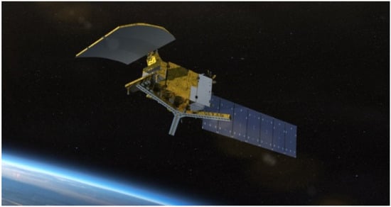
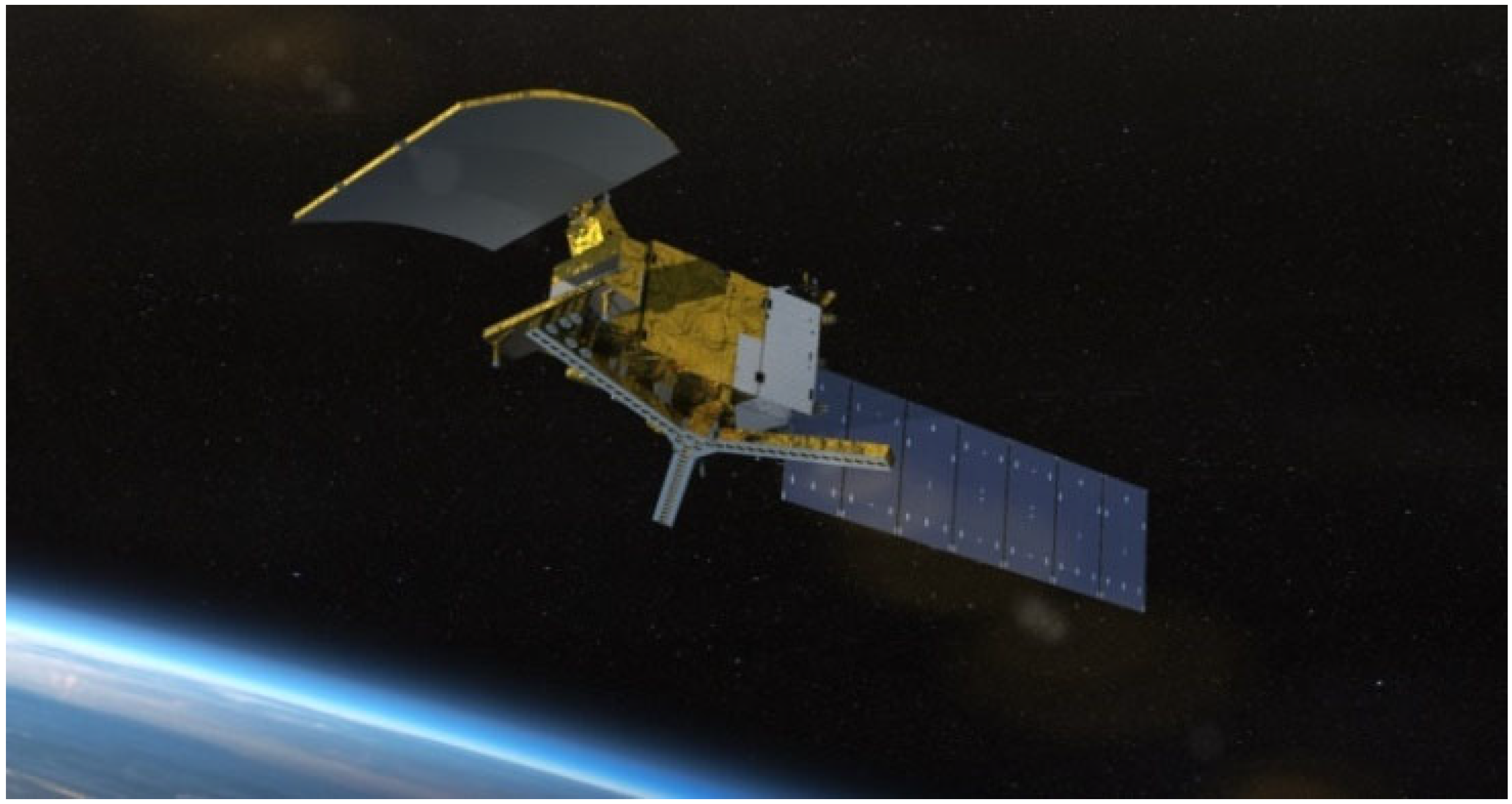
The COSM satellite was launched into orbit on 14 November 2024 by the Long March-4C (CZ-4C) carrier rocket from the Taiyuan Satellite Launch Center in China, as shown in Figure 1. The satellite is based on the ZY2000 Remote Sensing Satellite Platform (ZY2000 Platform) developed by CAST. This platform is universal and adaptable, with technical characteristics such as agile maneuvering control, highly accurate positioning support, integrated vibration control, and a general-purpose onboard data system. It can be applied to various high-precision and high-efficiency low-orbit remote sensing missions [7].
Figure 1.
Chinese Ocean Salinity Mission in orbit.
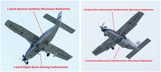
COSM was equipped with two payloads to obtain ocean salinity information, namely an L-band Aperture Synthesis Microwave Radiometer (LASMR, China Academy of Space Technology, Xi’an, Shaanxi, China) and Microwave Imager Combined Active and Passive (MICAP, National Space Science Center, Beijing, China). During the development of the payloads, their prototypes were carried on a plane to test their performance, as shown in Figure 2. The aerial experiment obtained salinity information from an offshore sea area and generated grid products. For a geographical grid with a side length of 100 m, the optimal accuracy of salinity data is about 1.2 psu from a single payload, and the best accuracy for joint inversion can reach 1 psu for two payloads, verifying the effectiveness of the working mechanism for satellite payloads [8].
Figure 2.
The aerial experiment for the payloads of COSM.
2.1. Imaging Principle
The two radiometers of COSM scan the Earth’s surface with interferometry and aperture synthesis technology, which is based on antenna arrays, to measure the frequency domain from L-band radiation, instead of using a traditional real aperture radiometer. The spatial resolution of the real aperture antenna during measurements is proportional to the antenna size. For the same spatial resolution, the lower the microwave radiation frequency measured in different bands, the larger the necessary antenna size. If the required spatial resolution for measuring in the L-band is 100~200 km, the real aperture antenna size far exceeds the carrying capacity of the rocket. For an aperture synthesis radiometer antenna array, any pair of its antenna feed sources can perform interferometry for radiation in the field of view. When the interferometry results are put together from all pairs of feed sources, transforming the frequency domain data into brightness temperature data using a mathematical method, the antenna array is equivalent to a large aperture antenna when observing radiation from the ocean [9].
The aperture synthesis radiometer is essentially different from a traditional microwave radiometer in principle. For antenna, aperture synthesis radiometers have “pairs of feed sources” with different baseline lengths that perform interferometry to measure the frequency domain from radiation. The baselines of various lengths and directions sample the spatial frequency domain from low to high frequencies, yielding the visibility function of the scene. For the retrieval algorithm, each point in the frequency domain has a physical meaning, and the corresponding brightness temperature image can be mapped onto the scene plane using Inverse Fourier Transform or other mathematical methods.
2.2. L-Band Aperture Synthesis Microwave Radiometer (LASMR)
LASMR adopts a Y-shape antenna array with a two-dimensional aperture synthesis system, which is designed and manufactured by the Xi’an Branch of CAST in Xi’an. It is mainly composed of an antenna sensing head, a digital correlator, and a low-frequency cable, which can measure L-band radiation from all directions in the view [10]. The digital correlator and sensing head (including the antenna array, receiver, and calibration network) are respectively installed inside and outside cabin, and are connected through the low-frequency cable. The antenna sensing head receives radiation energy and transmits a signal to the digital correlator.
The antenna array consists of the central antenna, left deployable arm, fixed arm, and right deployable arm. The central antenna is equipped with eight feed sources and each of the three antenna arms is equipped with 16 feed sources; the entire Y-shaped antenna has a total of 56 feed sources. When the antenna points towards the Earth’s surface, each feed source can receive radiation signals from the Earth’s surface. The receiver will amplify and filter radiation signals and down-convert them to intermediate frequency signals. The multi-channel intermediate frequency signals are collected, modulated (in-phase and quadrature), and subjected to multi-correlation processing by the digital correlators. Finally, multi-channel digital signals are multi-correlated in pairs and transmitted to the satellite computer [11]. The calibration network provides calibration signals to the receiver, achieving periodic internal calibration of the receiver.
LASMR can provide L-band brightness temperature at a high resolution and high sensitivity, along with multi-incidence data to measure ocean salinity and soil moisture [12]. The specifications of LASMR are shown in Table 3.
Table 3.
The key specifications of LASMR.
2.3. Microwave Imager Combined Active and Passive (MICAP)
The MICAP equipped for the COSM consists of an L/C/K-band One-dimensional Interferometric Microwave Radiometer (L/C/K-OIMR) and L-band Digital Beam-forming Scatterometer (LDBS). They share the same parabolic cylinder reflector in order to realize active and passive observation of the sea surface synchronously, and are designed and manufactured by NSSC in Beijing. For MICAP, the radiometer uses a one-dimensional aperture synthesis system, which is an antenna array composed of eight feed sources, and the scatterometer uses a phased array system, which is an antenna array composed of seven feed sources. The aperture synthesis array of the radiometer improves the resolution and view range for observing L-band radiation perpendicular to the flying direction, but it still uses a real aperture to observe the Earth’s surface in the flying direction, so MICAP must utilize the flight of satellites for imaging. The specifications of MICAP are shown in Table 4.
Table 4.
The key specifications of MICAP.
In the active and passive system, the radiometer has a wide-beam radar, and the resolution is improved by processing observation data. The scatterometer has a linear array radar, whose feed sources are deployed with equidistant distribution between the radiometer’s thinned arrays, and scans the sea surface perpendicular to the orbit direction with a digital beam forming. The scatterometer utilizes linear frequency modulation signals to obtain range resolution and can perform push-broom scanning at the same level (more than 950 km) as the radiometer [13]. The scatterometer and radiometer work together; when the scatterometer is in the transmitting state, the radiometer receiver enters the protected mode (input terminal switched to internal matched load), but both work simultaneously at other times.
MICAP can not only obtain sea surface salinity information, but can also observe auxiliary information simultaneously, such as sea surface roughness and temperature, and can detect and suppress Radio Frequency Interference (RFI) [14,15]. RFI refers to electromagnetic radiation interference from human activities. Although the L-band (1400~1427 MHz) is a microwave band specifically allocated for passive remote sensing internationally, illegal or unintentional interference still exists in reality, which pollutes the measurement signals of radiometers observing ocean salinity.
3. Routine Operation
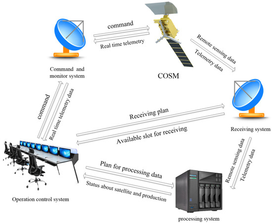
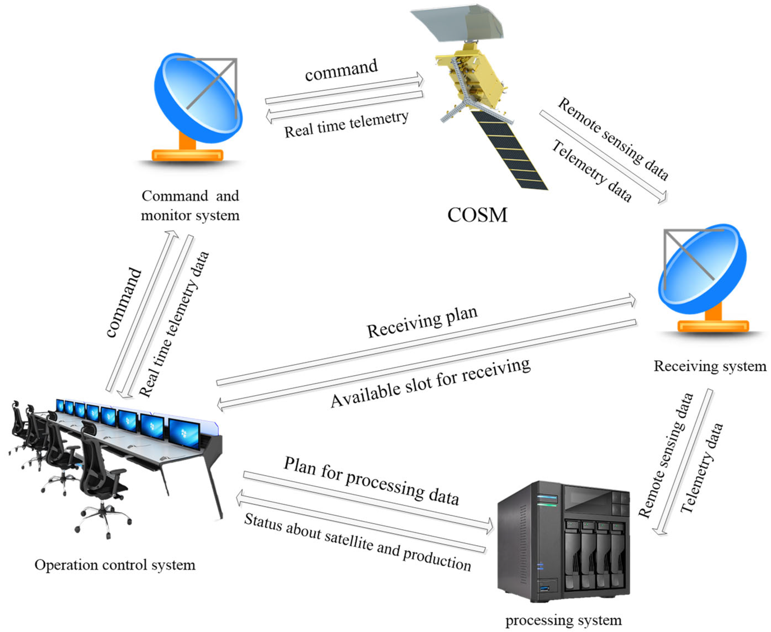
After the COSM satellite is in orbit, ground segment will serve as its control, receiving and processing data. The ground segment includes an operation control system, command and monitor system, receiving system, and processing system. The operation control system is the core of the ground segment, and is mainly responsible for initiating tasks and coordinating the other three systems, monitoring the satellite and ground segment, triggering the processing system to produce remote sensing data, and establishing the closed-loop between the satellite and the ground segment. The framework of the ground segment of COSM is shown in Figure 3.
Figure 3.
The satellite and its ground segment.
3.1. Control and Telemetry
The primary mission of the command and monitoring system includes telecontrol and telemetry. Telecontrol generates command data to control the satellite and sends them to the satellite, which is called uplink. Telemetry surveys the satellite to acquire its spatio-temporal parameters and receives real-time data about the satellite’s internal conditions, which is called downlink.
3.1.1. Uplink
Because the payload works for 24 h every day, these uplink commands mainly control the satellite transmission system in order to send remote sensing data to the ground receiving station or maneuver platform when the satellite is working properly. The command and monitoring system of COSM sends instructions to the satellite twice every week. The satellite communicates with the ground 3 to 4 times for data transmission per day, following ground commands. The commands to maneuver the satellite can be uploaded as required when the satellite is over tracking station.
Besides the above-mentioned commands, according to scheme and schedule, the command and monitoring system will also send command data to the satellite for maintenance regularly.
3.1.2. Downlink
When COSM is working, the command and monitoring system can attain spatio-temporal information when the satellite passes over the tracking station and can calculate the orbit elements of the satellite based on them. The orbit element is fundamental for predicting the range for data transmission from the satellite, and is a necessary condition for making command data for the telecontrol.
When the satellite flies over the tracking station, the satellite will transmit real-time telemetry data to the command and monitoring system, which can monitor satellite conditions and send visual and digitized information to the operation control system.
3.2. Receiving
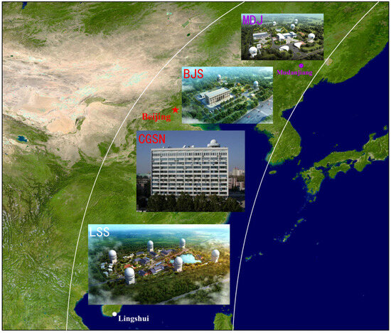
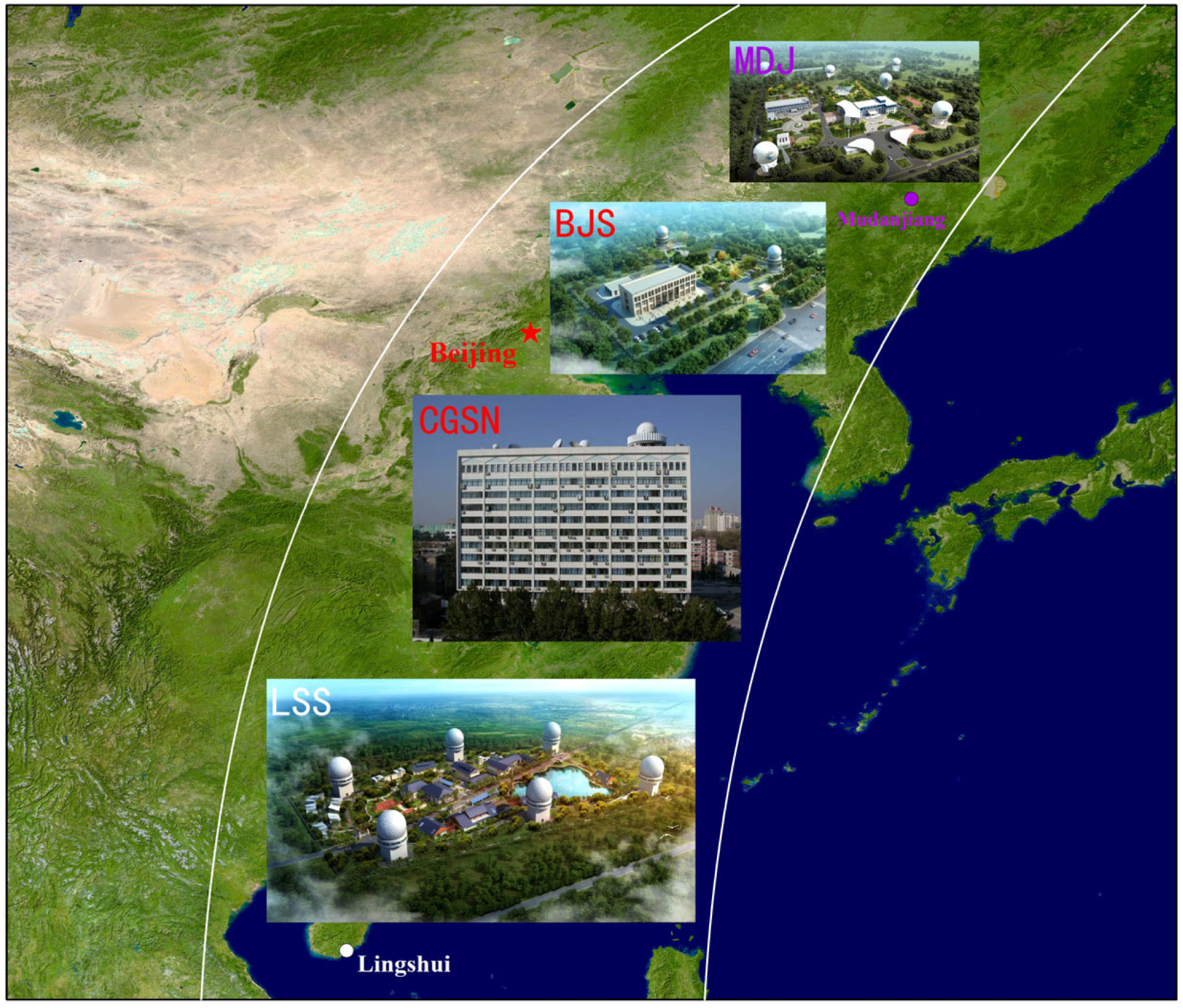
Receiving is how the remote sensing and telemetry data recorded by the satellite-borne recorder are transmitted to the ground receiving system. The receiving system consists of three ground receiving stations distributed across China and the center of the ground station network (CGSN) in Beijing, as shown in Figure 4. After all data from the satellite have arrived at the ground level, every station will transmit them to the CGSN through special a network.
Figure 4.
The ground receiving system of COSM.
A receiving system is deployed from north to south in eastern China, including Mudanjiang Station (MDJ), Beijing Station (BJS), and Hainan Station (LSS). The real-time remote sensing data can be transmitted to the three stations synchronously when the satellite flies over the Western North Pacific.
The CGSN is located in Beijing and serves as the control center for the three ground stations. It has two main tasks: firstly, forecasting when the satellite will fly over every station and sending available slots to the operation control system to make a time schedule for receiving data; secondly, handing the time schedule from the operation control system to every station and scheduling them to complete downlinking.
3.3. Processing
Processing is when the COSM’s processing system makes raw remote sensing data from ground receiving stations into standard multiple-level product data. This process includes two main steps: preprocessing and inversion. The preprocessing converts electronic signals recorded from the satellite into brightness temperature data and then geolocation data. This inversion is performed in order to convert brightness temperature information into physical parameters, such as ocean salinity, sea surface temperature and soil moisture. Since the two radiometers of the COSM have same the working principle when observing the ocean, both methods of preprocessing these two sets of data are also quite similar. The product levels of COSM are shown in Appendix B.
3.3.1. Preprocessing for LASMR
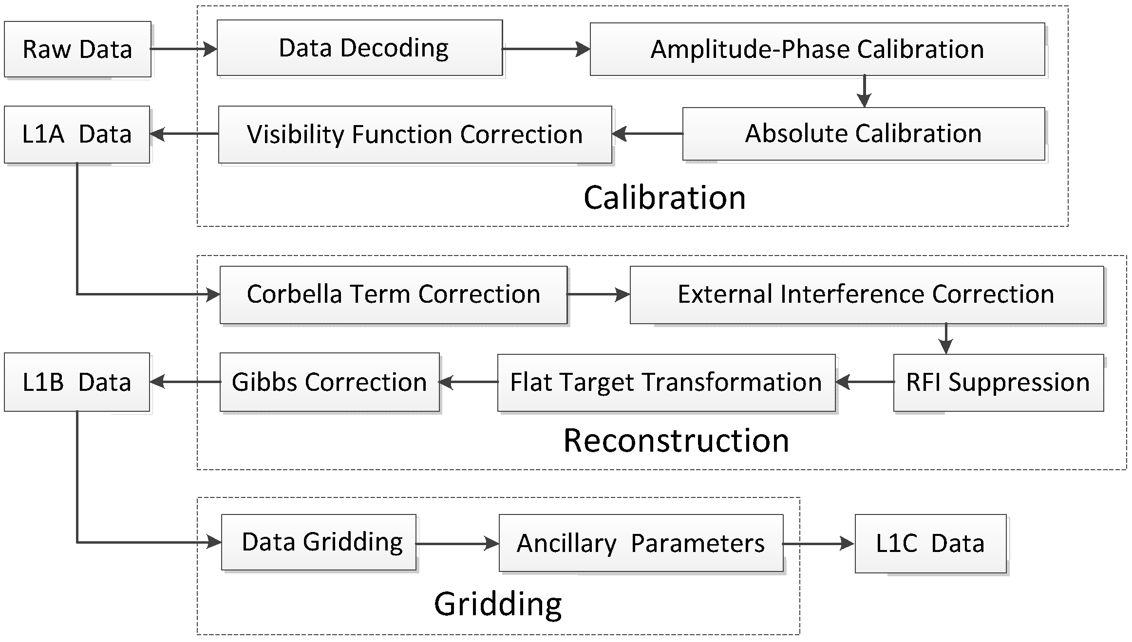
The preprocessing of remote sensing data for LASMR is divided into three stages, which include producing L1A data, L1B data, and L1C data, respectively, as shown in Figure 5.
Figure 5.
Data preprocessing chain of LASMR.
Producing L1A data involves calibrating the payload system and correcting the received raw data, outputting the visibility function as L1A data. Producing L1B data involves rebuilding brightness temperature values from L1A data and correcting for external error, outputting information about the brightness temperature distribution from the antenna aperture as L1B data. Producing L1C data involves geolocating and projecting brightness temperature values to the Earth’s surface using L1B data, outputting L1C data containing brightness temperature information with geographic coordinates.
3.3.2. Preprocessing for MICAP
The preprocessing of remote sensing data for L/C/K-OIMR is also divided into three stages, and the main tasks and products of every stage are similar to the preprocessing of remote sensing data for LASMR.
The preprocessing of remote sensing data for LDBS is divided into two stages, including producing L1A and L1B data, respectively.
Producing L1A data involves parsing and inspecting the received raw data and generating L1A data according to specifications. Its main tasks include extracting remote sensing data packets, auxiliary data packets, raw I/Q (in-phase/quadrature) data packets, and raw AD data packets, interpolating ephemeris data and attitude data about the satellite, and obtaining items with equal frame length.
Producing L1B data involves positioning and calibrating L1A data and generating L1B data that contains the backscatter coefficient from the sea surface and its geographic information according to the observation time. Its main tasks include geolocation, internal calibration, calculating the SNR (Signal-to-Noise Ratio) and backscatter coefficient, clearing FRE (Faraday Rotation Effect), etc.
3.3.3. Inversion
There are two main products from the observed COSM data: ocean salinity and soil moisture. The retrieval model for ocean salinity includes an integrated model and phased model. The retrieval model for soil moisture is an independent model whose method is similar to that of the ocean salinity integrated model.
The integrated model is a cost function whose expression mainly includes output target variables, observed input data from COSM, prior data, and forward model output data, as shown in Equation (1). The cost function stops iterating when the best fitting curve is obtained, and the optimal values for the output target variables become sea surface salinity, temperature, wind speed, water vapor and other information. The observed input data include brightness temperature from the two radiometers and the backscattering coefficient from the L-band scatterometer. The prior data can come from multiple sources, and their brightness temperature and backscattering coefficients come from the forward model.
In the equation, is the cost function; and are observed brightness temperature and the backscattering coefficient; and are the sensitivities of the radiometers and scatterometer; shows the weight of target variables and is a function of payload sensitivity, inversion model error, and initial field error; and and are the numbers for and in each geographic grid. In the subscript, and show the L-band radiometers of LASMR and MICAP, and show the C-band and K-band radiometers of MICAP, and show the polarization of the radiometers, shows the data from forward model, and show the polarization of the scatterometer, , , , and are the target variables of sea surface salinity, temperature, wind speed, and vapor, respectively, and shows that they are prior data.
The phased model includes three similar cost functions, as shown in Equation (2). Firstly, sea surface temperature and wind speed can be removed from Equation Χ(SST) and Equation Χ(WS), respectively, and are imported into the forward model using prior salinity data, which can be used to obtain brightness temperature data. The observed sea surface salinity will be obtained from Equation Χ(SSS).
In these equations, and are the uncertainty of the observed values from the radiometer and scatterometer, is the prior error, and is the number of or .
4. Calibration
The microwave radiometer can obtain accurate brightness temperature information from the Earth’s surface through calibration, which is an essential method for quantitative remote sensing. The synthetic aperture microwave radiometer of COSM consists of multiple radiometer antenna feeds; compared with the traditional radiometer, its calibration is extended from a single receiver to all receiving units.
The calibration for the radiometers of COSM consists of internal calibration and external calibration. The purpose of internal calibration is to calibrate the amplitude and phase inconsistencies among multiple links in the system by observing internal calibration signals periodically during orbit. The purpose of external calibration is to perform full-chain calibration and correction of Earth observation data from the radiometer by observing targets with known radiation intensity [16].
Because of the differences in the working mechanisms of LASMR and MICAP, their internal calibration processes are also different. However, the external calibration processes for these two radiometers are basically the same and include cold sky calibration. During cold sky calibration, the satellite rotates with respect to the satellite body coordinate system, and the two radiometers will measure the brightness temperature of a fixed point of background cold sky.
In December 2024, the COSM satellite performed its first maneuver for cold sky calibration. Remote sensing data were obtained by direct emission from the celestial sky to calibrate the two radiometers of the COSM. During this cold sky calibration, the satellite flew in ascending orbit, from the southwest hemisphere to the northeast hemisphere over the Pacific Ocean. The maneuver lasted for about 100 min from beginning to end, with stable observation of the cold sky for about 20 min. To ensure the safety of the whole satellite system, the satellite conducted two rolls before this maneuver in slots for telemetry in order to observe its state, showing normal control of the satellite’s attitude.
From January to April 2025, the satellite conducted three additional cold sky calibration observations, obtaining valid data that were used for the absolute calibration and Flat Target Transformation (FTT) of two payloads. This process effectively corrected the observed brightness temperatures. However, unexpected issues arose during the calibration operations. For instance, the two payloads had different observation methods, leading to irreconcilable conflicts in the constraints proposed for the calibration. It was difficult to ensure that a calibration maneuver could fully meet the requirements of both payloads simultaneously. Additionally, periodic variations in space objects sometimes increased interference sources, making the constraints for the calibration even more stringent. In response, future cold sky calibration efforts will adjust their operations by conducting calibrations for the two payloads separately based on actual conditions.
5. Conclusions
From its successful launch to October 2025, the ocean salinity satellite has maintained normal in-orbit operation, forming a closed-loop working system with the ground segment and establishing a stable, integrated space–ground workflow. However, during the satellite’s operation, the research team encountered several challenges.
First, the observation accuracy of the satellite’s payload still has room for improvement. This is primarily because the synthetic aperture microwave radiometer on the salinity satellite differs from traditional microwave radiometers. The process of converting observed electrical signals into brightness temperature signals involves a highly complex multi-stage procedure, which is the main reason for the difficulty of brightness temperature error correction. Additionally, interference from external noise sources cannot be entirely eliminated. Therefore, the research team needs to accumulate more data to continuously optimize the calibration algorithm.
Second, the ground system requires a relatively long time to process the observation data. This is mainly due to the complex data processing workflow of the synthetic aperture radiometer, as well as the increased data volume caused by the two-dimensional synthetic aperture radiometer’s multi-angle observations of the same target. To address this, the ground system has already deployed cluster computing for the salinity satellite’s data processing, which demands significant hardware resources.
The synthetic aperture radiometer used for measuring ocean salinity and soil moisture is a novel type of payload. Both its satellite and ground systems possess substantial application potential, but further time is needed for iterative upgrades in both software and hardware.
Author Contributions
Conceptualization, X.M. and W.Z.; validation, N.D. and X.Y.; writing—original draft preparation, X.M.; writing—review and editing, X.M.; visualization, Z.C.; supervision, W.Z.; project administration, W.Z. All authors have read and agreed to the published version of the manuscript.
Funding
This research was supported by the National Natural Science Foundation of China (funding number: 42376180).
Data Availability Statement
The data presented in this paper are available from the corresponding author upon reasonable request.
Conflicts of Interest
The authors declare no conflicts of interest.
Appendix A
The products of COSM can be downloaded via two methods: https://osdds.nsoas.org.cn/OceanDynamics (accessed on 5 July 2026) and ftp://osdds-ftp.nsoas.org.cn (accessed on 5 July 2026). The satellite is abbreviated as HY-4A in COSM. Before acquiring products via either method, users are required to register on the webpage of the above URL, as shown in Figure A1. This webpage supports both Chinese and English interfaces, which can be toggled by clicking the language switch icon in the upper-right corner of the webpage.
Figure A1.
The webpage to register and download.
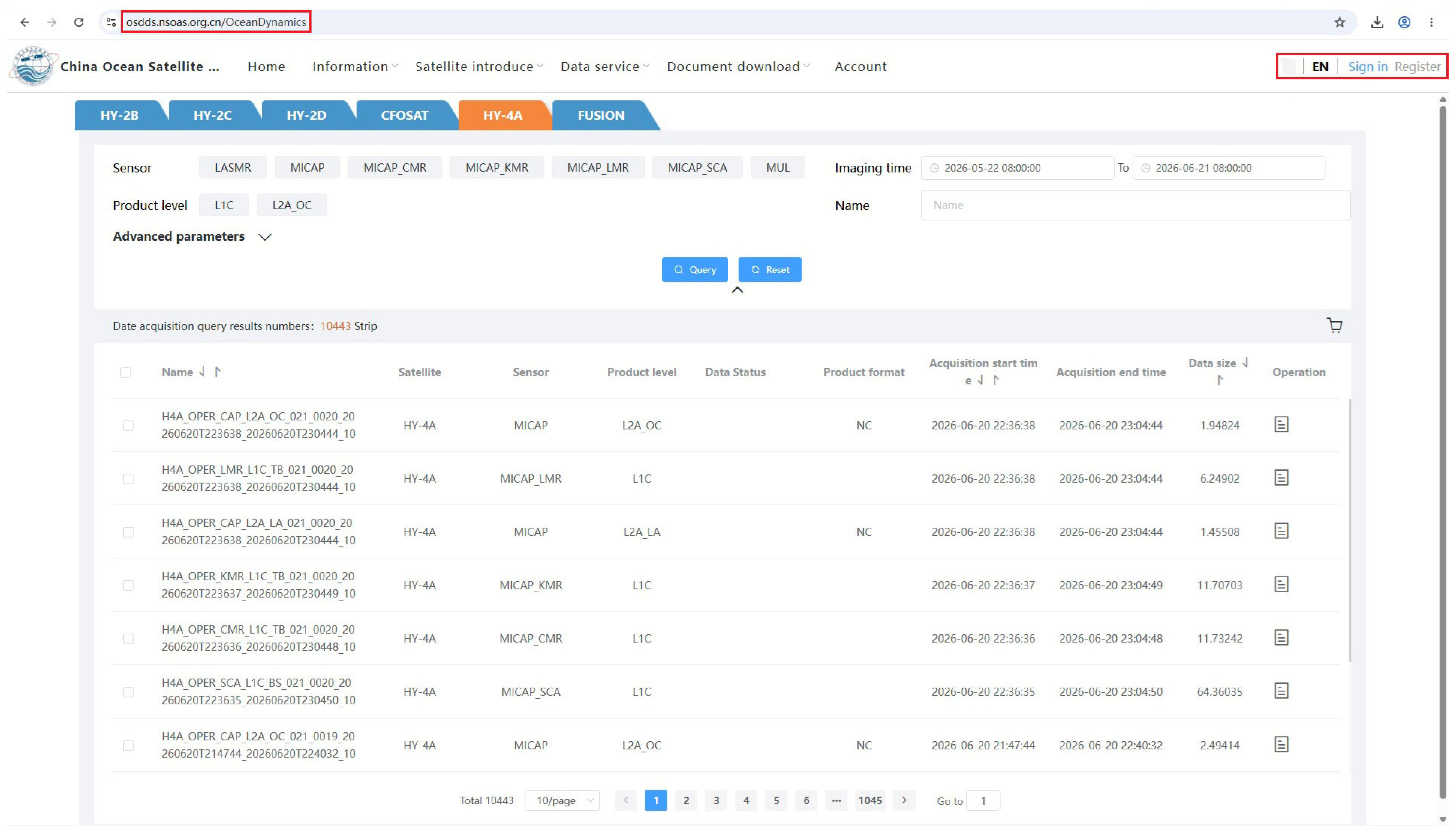
Users can download documents about the data format and programs for reading binary data and using data products via https://osdds.nsoas.org.cn/home (accessed on 5 July 2026) without registration or login, but the data format documents only have a Chinese version at present.
Appendix B
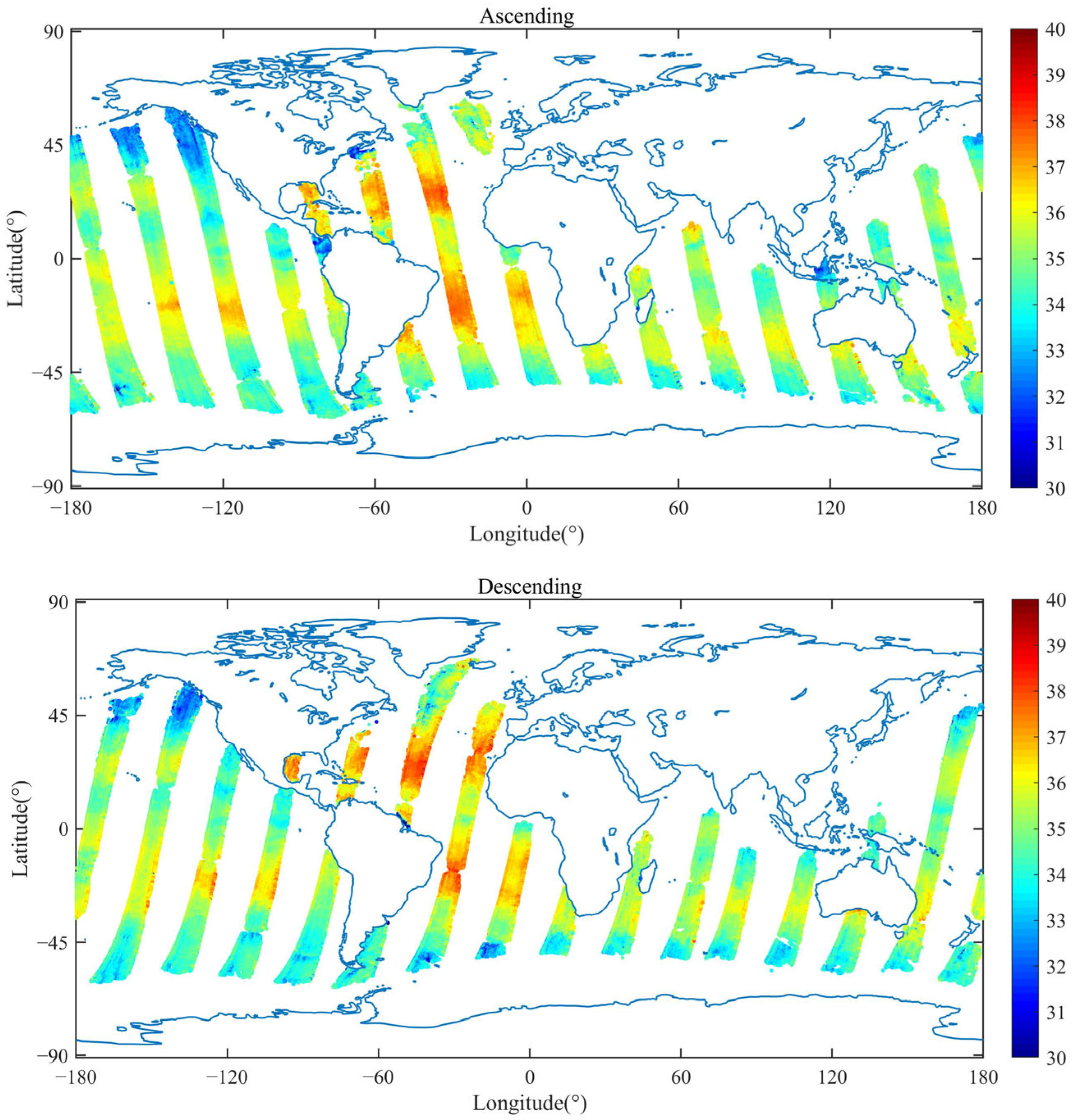
The publicly released and downloaded ocean products and land products include brightness temperature products (L1C) and inversion products (L2), whose types are shown in Table A1. The example map of ocean products (L2) is shown in Figure A2.
Table A1.
The types of products released by COSM.
Figure A2.
The example map of ocean products (L2, ascending and descending).
References
- Yang, Y.; Liu, Y.; Wang, Y.; Zhang, H.; Zhang, L. Dynamic modeling and motion control strategy for deep-sea hybrid-driven underwater gliders considering hull deformation and seawater density variation. Ocean Eng. 2017, 143, 66–78. [Google Scholar] [CrossRef] [Scilit]
- McDougall, T.J.; Jackett, D.R.; Millero, F.J.; Pawlowicz, R.; Barker, P.M. A global algorithm for estimating Absolute Salinity. Ocean Sci. 2012, 8, 1123–1134. [Google Scholar] [CrossRef] [Scilit]
- Lee, J.K.; Hirayama, K. Effects of salinity, food level and temperature on the population growth of Noctiluca scintillans (Macartney). Bull. Fac. Fish. Nagasaki Univ. 1992, 71, 163–168. [Google Scholar]
- Schwinger, J.; Tjiputra, J. Ocean carbon cycle feedbacks under negative emissions. Geophys. Res. Lett. 2018, 45, 5062–5070. [Google Scholar] [CrossRef] [Scilit]
- Camps, A.; Font, J.; Vall-Llossera, M.; Gabarro, C.; Corbella, I.; Duffo, N.; Torres, F.; Blanch, S.; Aguasca, A.; Villarino, R.; et al. The WISE 2000 and 2001 field experiments in support of the SMOS mission: Sea surface L-band brightness temperature observations and their application to sea surface salinity retrieval. IEEE Trans. Geosci. Remote Sens. 2004, 42, 804–823. [Google Scholar] [CrossRef]
- Lagerloef, G.S.E.; Swift, C.T.; Levine, D.M. Sea Surface Salinity: The Next Remote Sensing Challenge. Oceanography 1995, 8, 44–50. [Google Scholar] [CrossRef] [Scilit]
- Yu, L.; Gao, Y.; Zhang, G.; Yang, G.; Hao, X.; Chen, H. Features and Applications of ZY2000 Remote Sensing Satellite Platform. Spacecr. Eng. 2021, 30, 20–26. [Google Scholar]
- Li, Y.; Li, P.; Yang, X.; Li, G.; Chi, J.; Song, G.; Wang, C.; Wu, Y.; Liu, S.; Jiang, R.; et al. On Aperture Synthesis of Microwave Radiometer Demonstrator for Airborne 2-D L-Band and Ocean Aviation Applications. IEEE Trans. Geosci. Remote Sens. 2025, 63, 5302114. [Google Scholar] [CrossRef] [Scilit]
- Boutin, J.; Waldteufel, P.; Martin, N.; Caudal, G.; Dinnat, E. Surface Salinity Retrieved from SMOS Measurements over the Global Ocean: Imprecisions Due to Sea Surface Roughness and Temperature Uncertainties. J. Atmos. Ocean. Technol. 2004, 21, 1432–1447. [Google Scholar] [CrossRef] [Scilit]
- Li, Y.; Lv, R.; Song, G.; Yang, X.; Lu, H.; Li, P.; Tan, Q. FPASMR: A new instrument for future sea surface salinity measurement. In Proceedings of the IEEE International Geoscience and Remote Sensing Symposium, Fort Worth, TX, USA, 23–28 July 2017. [Google Scholar]
- Song, G.; Yang, X.; Li, Y.; Li, P.; Lu, H. The stability test of radiometer. In Proceedings of the IEEE International Geoscience and Remote Sensing Symposium, Fort Worth, TX, USA, 23–28 July 2017. [Google Scholar]
- Li, Y.; Li, H.; Liu, R. System design and analysis of L-band aperture synthesis microwave radiometer. In Proceedings of the IET International Radar Conference, Xi’an, China, 14–16 April 2013. [Google Scholar]
- Niu, L.; Liu, H.; Wu, L.; Zhang, C.; Zhao, X.; Wu, J.; Yin, X. Development and Experimental Study on L-band Synthetic Aperture Radiometer Prototype for Ocean Salinity Measurement. J. Electron. Inf. Technol. 2017, 39, 1841–1847. [Google Scholar]
- Zhang, L.; Jin, R.; Zhang, Q.; Wang, R.; Zhang, H.; Wen, Z. Fusion Method of RFI Detection, Localization, and Suppression by Combining One-Dimensional and Two-Dimensional Synthetic Aperture Radiometers. Remote Sens. 2024, 16, 667. [Google Scholar] [CrossRef] [Scilit]
- Han, D.; Tong, X.; Huo, C.; Ma, H.; Guo, X.; Li, B. Experimental Flight Verification of Radio Frequency Interference Mitigation Method in MICAP L-Band Radiometer. In Proceedings of the IGARSS 2024-2024 IEEE International Geoscience and Remote Sensing Symposium, Athens, Greece, 7–12 July 2024; pp. 9174–9177. [Google Scholar]
- Li, Y.; Li, H.; Lv, R.; Li, Y. SMOS Orbital Calibration. Space Electron. Technol. 2012, 9, 20–25+36. [Google Scholar]

Disclaimer/Publisher’s Note: The statements, opinions and data contained in all publications are solely those of the individual author(s) and contributor(s) and not of MDPI and/or the editor(s). MDPI and/or the editor(s) disclaim responsibility for any injury to people or property resulting from any ideas, methods, instructions or products referred to in the content. |
© 2026 by the authors. Licensee MDPI, Basel, Switzerland. This article is an open access article distributed under the terms and conditions of the Creative Commons Attribution (CC BY) license.