


Highlights
What are the main findings?
- A dynamic error model yields more consistent thermodynamic adjustments and improved cloud analysis, particularly for convective structures.
- The dynamic error model performs better when solid-phase hydrometeors are included as control variables, allowing their direct update in ASR assimilation.
What are the implications of the main findings?
- Accounting for cloud-related uncertainties using a cloud-impact-dependent observation error model is essential for successful ASR assimilation.
- Including all hydrometeor species in the control variables is critical for accurately representing cloud and precipitation processes.
Abstract
Assimilation of all-sky radiance (ASR) observations informs atmospheric states and cloud distributions; however, it does not always lead to improved analyses or forecasts. In particular, directly updating hydrometeor fields introduces substantial uncertainty into ASR assimilation. This study examines the impact of dynamic observation errors on analyses and precipitation forecasts under different hydrometeor control variable (HCV) configurations. Observation errors are prescribed using a fifth-order polynomial model as a function of a cloud impact parameter, allowing spatiotemporally varying (i.e., scene-dependent) errors that adapt to cloud conditions. Results indicate that dynamic observation errors generally improve cloud analyses and associated thermodynamic fields. By contrast, constant errors tend to overweight ASR observations in heavily cloud-affected regions, thereby degrading analysis quality. The advantages of dynamic errors are more pronounced when solid-phase hydrometeors are included in the HCV, as these strongly influence brightness temperature (BT) analysis and the representation of convective cloud tops. Among all experiments, those combining dynamic errors with direct updates of solid-phase hydrometeors produce the most realistic BT and reflectivity analyses, as well as the greatest improvements in precipitation forecasts. These results underscore the importance of cloud-dependent observation error modeling in ASR assimilation, particularly when solid-phase HCVs are employed.
1. Introduction
Advances in computational power have made high-resolution numerical modeling of atmospheric phenomena across various scales feasible. However, due to discrepancies between numerical models and reality, assimilating observational data remains essential for producing accurate forecasts in the inherently chaotic atmosphere [1,2,3,4]. Satellite observations offer valuable information over oceanic regions—where conventional observations are sparse—as well as in clear-sky areas not captured by radar. Accordingly, assimilating satellite data into numerical models can improve forecasts of high-impact weather events.
Previous studies have demonstrated the benefits of assimilating clear-sky radiance (CSR) data for forecast accuracy [5,6,7]. More recent research has highlighted the advantages of extending beyond clear-sky-only assimilation to incorporate cloud-affected radiances within a unified framework [8,9,10,11,12,13,14,15,16]. In cloud-affected areas, assimilation becomes more challenging, owing to increased inter-channel error correlations [17], uncertainties from radiative transfer model (RTM) errors, and representativeness errors due to cloud mismatches [18]. Therefore, effective assimilation of all-sky radiance (ASR) requires explicit treatment of additional cloud-related uncertainties [19,20,21,22,23,24].
One widely used approach is dynamic observation error modeling, in which observation errors are prescribed as functions of scene-dependent cloud characteristics rather than fixed constant values. A symmetric cloud-effect parameter has been proposed for microwave brightness temperature (BT) observations, with observation errors modeled as a function of this parameter [25]. Subsequently, a cloud-effect parameter for infrared BT observations was developed and shown to be closely related to the standard deviation (STD) of first-guess (FG) departures (observation minus background, O–B) [26]. These cloud-effect predictors have demonstrated potential for cloud-dependent quality control (QC) and for characterizing observation errors. However, limitations associated with the use of background BT within the observation component of the cloud parameter have been identified. To address this issue, an alternative parameter based on threshold BT values has been proposed, along with an approach to estimate observation errors by excluding model error components derived from ensemble forecasts [18].
Hastuti [27] developed an observation error model for ASR from the water vapor (WV) channels on Korea’s GK-2A (Geostationary Korea Multi-Purpose Satellite-2A) AMI (Advanced Meteorological Imager), fitting statistically derived O–B STDs to a higher-order regression function of the cloud parameter from [26]. Data assimilation (DA) experiments using real cases showed that this method outperformed the piecewise linear function proposed by [25]. However, their work did not fully analyze the differences between the two error models in prescribed errors during cycling, nor their relative impact on assimilation accuracy. Thus, further analysis is required to clarify how spatiotemporal variability in observation errors contributes to improvements in analysis and forecast fields. In this context, the present study investigates the evolution of observation error distributions throughout the cycling process and their influence on the analysis field in space and time. By comparing a simple constant-error model with a higher-order regression model—rather than two variable models as in [27]—this study enables a clearer contrast in error magnitudes and their respective impacts. The results also offer a reinterpretation of [27], contributing to a more consistent understanding of GK-2A AMI ASR assimilation effects.
Additionally, there remains a need to reevaluate the impact of observation error models when solid-phase hydrometeors are included as control variables (CVs)—an aspect not addressed in previous GK-2A AMI assimilation studies. The choice of CVs can substantially affect the analysis field [28,29,30,31], while ASR simulations are also sensitive to the representation of upper-level hydrometeor types [32]. These sensitivities, together with the strong nonlinearity associated with cloud-affected radiances and solid-phase microphysical processes, have made the direct update of solid-phase hydrometeors through radiance assimilation challenging. Nevertheless, recent studies have increasingly highlighted the importance of hydrometeor-aware DA frameworks. For example, Shen [33] showed that hydrometeor CVs helped suppress false echoes and improve precipitation forecasts in radar reflectivity assimilation. More recently, Yang [34] demonstrated that a full-hydrometeor 4D-Var framework incorporating ice-phase hydrometeors as CVs provided a more physically consistent initial state, reduced model spin-up time, and improved short-term precipitation forecasts. These recent findings further motivate the present investigation of solid-phase hydrometeor updates in GK-2A AMI ASR assimilation. Because hydrometeor updates are strongly influenced by cloud-affected radiances, dynamic observation error modeling is also expected to play an important role in this framework.
Therefore, this study also aims to assess changes in GK-2A AMI ASR assimilation performance when solid-phase hydrometeors are incorporated as CVs and to examine how dynamic observation errors interact with these updates during the assimilation cycle. Furthermore, since [27] did not evaluate hydrometeor changes, the present work provides added value by examining hydrometeor updates induced by GK-2A AMI ASR assimilation.
2. Materials and Methods
2.1. Model Configuration and Data Assimilation Setup
In this study, the Weather Research and Forecasting model (WRF-ARW) Version 4.2.1 was utilized [35]. The model configuration featured 60 vertical levels with a model top set at 50 hPa and consisted of two domains with horizontal resolutions of 9 km (D01) and 3 km (D02), respectively (Figure 1). Detailed information on the physical parameterizations and the overall model setup is provided in Table 1.
Figure 1.
WRF domain configuration with terrain height (m). The outer and inner red boxes indicate D01 and D02, respectively.
Table 1.
WRF configuration.
For DA, the three-dimensional variational (3DVAR) method implemented in the WRF Data Assimilation (WRFDA) Version 4.2.1 system was utilized [31,44,45]. This method obtains an analysis state by iteratively minimizing a cost function that incorporates both the observational data and the model background state , along with their respective error covariance matrices. The cost function J of the 3DVAR method is expressed as follows in Equation (1).
and denote background error covariance matrix and the observation error covariance matrix, respectively. Operator , which appears in the observational term of the cost function, is the observation operator that facilitates comparison between model values and observations in the same spatiotemporal domain and units. In satellite DA, the RTM serves as the observation operator. The RTM computes radiance (expressed as BT)—a variable not directly predicted by the WRF model—thereby enabling the generation of analysis increments through comparison with observations. In this study, the Community Radiative Transfer Model (CRTM) Version 2.3.0, developed by the Joint Center for Satellite Data Assimilation (JCSDA), was employed as the RTM [46].
2.2. Data for Assimilation and Validation
Launched in December 2018, South Korea’s GK-2A succeeded the Communication, Ocean, and Meteorological Satellite (COMS-1) and currently conducts meteorological observation missions. The AMI onboard GK-2A observes 16 channels: four visible, two near-infrared, and ten infrared (IR). These spectral bands are comparable to those of the Advanced Himawari Imager (AHI) on Himawari-8 and the Advanced Baseline Imager (ABI) on the Geostationary Operational Environmental Satellite-16 (GOES-16).
The three WV channels, corresponding to AMI channel numbers 8–10 (6.3, 6.9, and 7.3 µm), are sensitive to mid- and upper-tropospheric WV and thus provide valuable information on atmospheric moisture. For this study, ASR data from these three WV channels of the GK-2A AMI Level 1B product (available at 10 min temporal and 2 km spatial resolution) were assimilated. ASR data were converted to BT using conversion tables provided by the National Meteorological Satellite Center prior to assimilation. For BT validation at the final cycling step, additional observations from channel 14 (11.2 µm, an atmospheric window channel) were used. All BT data were thinned to 9 km resolution to match Domain 1 grids.
In addition to ASR, GK-2A Level-2 Atmospheric Motion Vector (AMV) data (available at 10 min temporal resolution) from all channels were assimilated, together with observations from Automatic Weather Stations (AWS), the Automated Synoptic Observing System (ASOS), ocean platforms, radiosondes, and wind profilers.
Reflectivity analyses were verified using gridded Constant Altitude Plan Position Indicator (CAPPI) data derived from Korean radar Plan Position Indicator (PPI) observations. These PPI datasets were merged and interpolated to a constant height using a previously developed algorithm [47,48,49]. The CAPPI output was then gridded at 3 km horizontal resolution to match that of the model’s inner domain. For hourly precipitation verification, we used the Integrated Multi-satellitE Retrievals for GPM (IMERG) Final Precipitation L3 product [50], which offers a spatial resolution of 0.1° × 0.1° and a temporal resolution of 30 min. To evaluate thermodynamic fields, hourly European Centre for Medium-Range Weather Forecasts (ECMWF) Reanalysis version 5 (ERA5) [51] pressure-level data with a spatial resolution of 0.25° × 0.25° were used, together with all available radiosonde observations over the Korean Peninsula at the corresponding times.
2.3. Model Background Error Covariance and ASR Observation Error Model
In this study, the model background error covariance ( in Equation (1)) was estimated using the National Meteorological Center (NMC) method, which derives statistics from the differences between forecasts valid at the same time but initialized at different lead times [52]. Following [53], statistics were computed from the differences between 12 and 24 h forecasts over the summer months (June–August) of 2017–2019, as expressed in Equation (2).
The zonal and meridional wind components (u and v), temperature (T), pseudo relative humidity (RHs), and surface pressure (Ps) were used to estimate the background error statistics. For hydrometeors, background error variances were not derived from the NMC method. Instead, spatially homogeneous background error variances and horizontal recursive-filter length scales were empirically prescribed for each hydrometeor species. A uniform variance amplitude of 5 × 10⁻⁷ (kg kg−1)2 was applied to all hydrometeor variables, based on preliminary sensitivity tests. Vertical correlations and multivariate cross-correlations were neglected, and only horizontal correlations were considered.
With the transition from CSR to ASR assimilation, efforts were made to model observation error variability based on the degree of cloud influence. Since error correlations are generally stronger in cloudy regions than in clear sky [7,10,17], observation error models were developed to inflate clear-sky observation errors according to the degree of cloud impact [18,25,26]. In this study, the cloud effect parameter proposed by [26] was used, as defined in Equation (3).
The parameters and represent the cloud impact from the model and observations, respectively. Specifically, is defined as , and as , where refers to the GK-2A observed BT, is the clear-sky BT calculated by the WRF-CRTM with hydrometeors excluded (i.e., assuming no cloud influence), and B is the BT computed with cloud effects. Consequently, larger values can occur when cloud structures are more realistically represented in the model. In such cases, increased observation errors reflect greater uncertainties associated with cloud-affected radiative transfer and observation operators.
Statistical values for , , , and the derived cloud impact parameter were obtained over Domain 1 (Figure 1) using GK-2A observations and 6 h short-range WRF forecasts for August 2023. To construct the observation error model, STDs of O–B were collected for each 1 K interval of (black lines in Figure 2). The error models for each WV channel were then derived by fitting these data using a fifth-order polynomial regression function of the form (blue lines in Figure 2, labeled “HE” for Higher-order regressed Error). This fitting approach follows [27] to maintain consistency with the previous GK-2A AMI ASR framework while extending the analysis to include the impacts of different HCV configurations.
Figure 2.
O-B BT statistics for GK-2A channels (a) 8 (6.2 µm), (b) 9 (6.9 µm), (c) 10 (7.3 µm), (d) 14 (11.2 µm), (e) 15 (12.3 µm), and (f) 16 (13.3 µm). Each panel shows the mean (black dashed line, K), STD (black solid line, K), constant-error model (CE; red line, K), and higher-order regressed-error model (HE; blue line, K) as functions of the cloud effect parameter , binned at 1 K intervals. Grey bars (right y-axis) indicate the number of data samples per bin.
This approach is supported by the notion that the average cloud impact parameter can be used to predict the STD of first-guess (FG) departures and is thus expected to serve as a suitable proxy for observation error (cf. [18]). While the FG departure STD () reflects the total error, it can be expressed as the root-sum-square of the forecast error () and the observation error () components (Equation (4)). This relationship holds under the assumption that observation and background errors are uncorrelated [25].
Since the FG departure STD includes , using this value directly as the observation error assumes the forecast error is sufficiently small. This assumption has been adopted in several previous studies [26,27,54], and accordingly, the present study also uses the raw STD values as observation errors without further adjustment. In addition, to prevent unrealistically small observation errors from being assigned in areas with strong cloud influence, the error values were capped at the maximum value of the fitted model beyond the point where the model reached its peak. These regions correspond to cases where the model successfully simulates clouds reaching higher altitudes. Such cases typically occur near the cores of convective systems, where sample sizes are relatively small yet show better agreement with observations than the broader, more uncertain cloud peripheries.
The derived error models closely follow the O–B STD distribution, with errors increasing alongside the cloud impact parameter in Figure 2. Among the WV channels, the largest STDs are found in the 7.3 µm channel, likely due to stronger surface influence and related uncertainties in surface parameters. Surface-sensitive IR channels, including 11.2 µm, 12.3 µm, and 13.3 µm, generally exhibit even greater STDs than the WV channels, likely for the same reason. The maximum observation errors for channels 8, 9, 10, 14, 15, and 16 are 13.2 K, 17.0 K, 20.3 K, 33.6 K, 31.8 K, and 25.0 K, respectively, with corresponding saturation thresholds of 16.6 K, 18.1 K, 21.1 K, 31.3 K, 30.3 K, and 26.0 K. Overall, the STD values are comparable to those in the GK-2A observation error models presented by [27], although this study’s values are lower by approximately 3 K, 5 K, and 7 K for channels 8, 9, and 10, respectively. The constant observation error values, calculated as the mean STD from the total O–B statistics, are 4.5 K, 6.2 K, and 8.2 K for channels 8, 9, and 10 (indicated by red lines labeled “CE” for Constant Error in Figure 2).
2.4. Bias Correction and Quality Control
Okamoto [10] analyzed the benefits of ASR assimilation relative to CSR and demonstrated that ASR assimilation yields more stable improvements in both the initial field and precipitation forecasts. However, they also emphasized that bias correction (BC) remains a challenging issue. DA systems generally assume unbiased observations; in practice, this assumption is often violated due to factors such as instrument calibration errors and uncertainties in RTM simulations over cloudy regions. To ensure positive assimilation outcomes, it is essential to appropriately correct these systematic biases within the system.
Recently, beyond offline BC methods applied to individual channels, many operational and research systems have adopted variational BC (VarBC), which incorporates bias terms into the cost function of variational DA and facilitates real-time correction [55,56]. In this study, VarBC was applied by adding a bias term to the 3DVAR cost function, expressed as a linear combination of predictors and their corresponding coefficients, enabling real-time correction for each channel during assimilation. The chosen predictors include layer thicknesses between 1000–300 hPa and 200–50 hPa, skin temperature, total column precipitable water, and the satellite scan angle, together with its squared and cubic terms.
For stable DA, an appropriate QC process is also vital to filter out observations with large O–B values. This study employed a cloud-dependent O–B QC method proposed by [57]. Specifically, observations were rejected if and . This approach permits retaining more observations in regions with strong cloud influence, even when their O–B values are relatively large, thereby increasing the amount of assimilated observational information. In addition, observations of mixed surface types, such as coastal regions, were excluded to reduce uncertainties associated with surface emissivity.
2.5. Experiments and Case Description
A total of five experiments were conducted to evaluate the impact of constant versus variable observation error models and to examine how these models influence DA performance under different hydrometeor control variable (HCV) configurations (Table 2). In the CONV experiment, only conventional observations—radiosondes, wind profilers, AMVs, and surface/marine observations—were assimilated, excluding ASR data [58,59]. When GK-2A ASR data were additionally assimilated, experiments were labeled HCV2 if solid-phase hydrometeors (graupel, snow, and ice) were included as CVs, and HCV1 if they were not. For each HCV configuration, two types of observation error treatments were applied. In the CE experiments, channel-wise mean STDs of one month of O–B BT were used as observation errors. In the HE experiments, observation errors were assigned using a polynomial regression model based on the cloud impact parameter . These experiments enabled a sensitivity analysis of observation error specifications under different solid-phase HCV configurations.
Table 2.
Experimental setup.
When solid-phase hydrometeors are included as CVs, the mixing ratios of ice, snow, and graupel are incorporated into the control vector of the cost function (Equation (1)). In HCV2, this facilitates direct initialization of these hydrometeors by generating analysis increments from the differences between model-computed and observed BT.
For the experimental cases, two stationary front events that produced significant precipitation over the Korean Peninsula were selected. Case 1 (25 July 2019, 0300 UTC–26 July 2019, 1200 UTC) involved the development of localized convective cells along a stationary front over the western seas and coastal regions of Korea. Following the formation of a band-shaped front over central Korea, the front gradually shifted southward (Figure 3a,b). Case 2 (3 August 2020, 0000 UTC–1200 UTC) featured convective systems developing over the Yellow Sea, accompanied by a front forming over inland regions, both of which contributed to widespread precipitation. Compared with Case 1, this event exhibited stronger convective activity overall, with more intense low-level winds driven by a synoptic pattern characterized by a high-pressure system to the south and a low-pressure system to the north (Figure 3c,d). Spin-up periods of 6 h and 3 h were applied to Cases 1 and 2, respectively, followed by assimilation every 30 min for seven cycles over a 3 h period. The different spin-up durations were determined by the fixed 6 h interval of the FNL initial conditions and the differing onset times of the target precipitation events (00 UTC for Case 1 and 21 UTC for Case 2).
Figure 3.
Korean Meteorological Administration (KMA) analysis charts. (a,c) Surface synoptic analyses. (b,d) 850 hPa frontogenesis parameter (shading, °C), geopotential height (blue contours, gpm), temperature (red contours, °C), and wind barbs (≥20 kt). Upper panels (a,b) correspond to Case 1 (0000 UTC 26 July 2019), and lower panels (c,d) to Case 2 (0000 UTC 03 August 2020).
2.6. Evaluation Metrics
Several metrics are used to quantitatively evaluate the analyses: root mean square error (RMSE), bias, and pattern correlation (PC). The formulas for RMSE (Equation (5)) and PC (Equation (6)) are presented below:
Here, , , and N represent the predicted value, observed value, and the total number of comparison points, respectively. The overbar (¯) denotes the mean, and and indicate the STDs of observations and predictions.
In addition, the Fraction Skill Score (FSS) is employed to assess the spatial agreement of BT analysis fields. The FSS is calculated by comparing the fraction of “hits” within a predefined neighborhood for both observed and predicted fields, providing a scale-aware performance metric. The FSS is particularly suitable for evaluating variables such as BT, which exhibit strong spatial variability, as it accounts for near-miss events within a defined neighborhood.
The FSS is defined in Equation (7):
where and represent the fractional coverage of events (e.g., exceeding a threshold) within a neighborhood around grid point , and N is the total number of grid points. The FSS ranges from 0 to 1, where 1 indicates perfect agreement and 0 indicates no skill. In this study, the neighborhood was defined as a 7 × 7 grid (i.e., ±3 grid points from each center point), and a threshold of 230 K was used to identify convective regions, following [15].
3. Results
3.1. BT, , and Observation Error Distribution
By applying the higher-order polynomial observation error model (HE), it becomes possible to assign observation errors that vary spatiotemporally, reflecting the evolution and movement of weather systems. Figure 4 presents the observed BT and the corresponding observation error for the 7.3 µm channel in Case 1. The observation errors vary according to the distribution of the cloud impact parameter at the given time. Notably, the dynamically assigned errors are larger than those in the CE experiment in regions of higher cloud impact (red areas in Figure 4d) and smaller in regions of lower cloud impact (blue areas in Figure 4d). This approach allows the system to place greater trust in, and make better use of, observations less affected by clouds—both in the model and in the observations themselves.
Figure 4.
BT (K) at 7.3 µm from (a) GK-2A observation and (b) WRF-CRTM simulation at 0000 UTC 25 July 2019. (c) Cloud effect parameter and (d) corresponding observation errors assigned at the same time.
Regions with large observation errors (i.e., high cloud impact) closely correspond to areas where the actual GK-2A observations show low BT. In some areas, however, the influence appears to originate from clouds represented in the model (e.g., northeast of Taiwan and over the southeastern Korean Peninsula).
Figure 5 presents the error statistics averaged over both cases and WV channels during cycling for each experimental group. Throughout the cycling period, the HE experiments assigned smaller observation errors than their CE counterparts (grey bars) over Domain 1 (Figure 5a). This is attributed to Domain 1 containing a larger number of pixels near clear-sky conditions, for which the HE experiment prescribes smaller observation errors, as shown in Figure 4d. In contrast, when statistics are calculated over Domain 2, where major weather systems develop, the HE experiment assigns larger observation errors on average. Additionally, the degree of observation error inflation during cycling was greater in HCV2 than in HCV1. This results from the term, a component of the cloud effect parameter (Equation (3)) used to determine observation error, tending to be larger in HCV2. This increase likely arises from more effective cloud generation in HCV2 due to direct initialization of solid-phase hydrometeors, which amplifies the difference between and . Conversely, the component of the showed neither a clear difference among experiments nor a consistent trend over the course of cycling. Despite the generally larger values in HCV2, the total number of assimilated radiances remained broadly comparable among the experiments throughout the cycling period after the application of the cloud-dependent QC, with differences generally around 1% (Figures S1 and S2).
Figure 5.
(a) Mean observation errors for BT (bars), averaged over the three AMI WV channels in Domain 1 throughout the cycling period (Orange: HCV1_HE; Blue: HCV2_HE; Grey: constant error). Solid lines and dashed lines represent the mean values of and , respectively. (b) BT and (c) CMAX RMSE for the background and analysis fields during the cycling period (Red: HCV1_CE, Orange: HCV1_HE, Sky blue: HCV2_CE, and Blue: HCV2_HE).
As shown in Figure 5b, BT analysis errors decrease more substantially in HCV2 than in HCV1, and in HE experiments compared to CE. During cycling, background BT errors tend to increase in both the HCV1 series and HCV2_CE. However, in HCV2_HE, the background BT RMSE slightly decreases from approximately 5.8 K to 5.5 K over the cycling period. At the final time step, both the background and analysis fields show the closest agreement with the observed BT in the following order: HCV2_HE, HCV2_CE, HCV1_HE, and HCV1_CE.
In HCV1, CE initially exhibits smaller errors than HE, but HE surpasses CE in later cycles. Similarly, in HCV2, HE yields better agreement with observations than CE for both background and analysis fields—except for the first guess at the second assimilation step—with the gap between experiments widening over time. These results suggest that the relative importance of observation error specification may vary depending on cycling configuration.
In addition to BT, column-maximum radar reflectivity (CMAX)—an independent dataset not directly assimilated—was examined for verification. Reflectivity in the model was computed using temperature, WV, and mixing ratios of rain, snow, and graupel, assuming spherical particles with constant density and an exponential size distribution. (Calculated RMSE includes errors arising from this simplified reflectivity observation operator.) Verification was limited to regions where observed reflectivity exceeded −15 dBZ, assumed to represent the threshold for precipitating echoes. Additional sensitivity tests using different reflectivity thresholds showed that the relative performance among the experiments remained generally unchanged. The observed CMAX distribution primarily corresponded to melting-layer altitudes between approximately 3 and 7 km.
Similar to BT error evolution, CMAX RMSE indicates that the HCV2 configuration outperformed HCV1. In HCV1, RMSE increased significantly during cycling, reaching nearly 38 dBZ in the final analysis, whereas HCV2 reduced this error to around 24 dBZ. Unlike BT RMSE, the difference between HCV2_CE and HCV2_HE remained relatively small over time. This suggests that information from precipitating hydrometeors in mid-to-lower layers of vertically developed convection (roughly 3–7 km)—which dominates the CMAX signal—is less sensitive to variations in ASR observation error specification. Previous studies have shown that the ABI WV channels, which are nearly identical to the GK-2A AMI WV channels, exhibit peak clear-sky weighting functions near approximately 350 hPa (Channel 8), 400 hPa (Channel 9), and 500 hPa (Channel 10). Under deep convective conditions with high-altitude ice clouds, however, the weighting functions of all three channels shift upward and peak near 200 hPa [60]. Therefore, ASR assimilation in the major convective regions of the present cases likely exerted a stronger influence on upper-tropospheric hydrometeors, whereas the observed CMAX signal was primarily associated with lower-altitude precipitating hydrometeors at approximately 3–7 km.
3.2. Changes in the Final Analyses
After DA, the final analysis field was examined to assess the cumulative impacts of different observation error treatments and HCV configurations applied during cycling. Figure 6 and Figure 7 present simulated BTs from the 11.2 µm atmospheric window channel of GK-2A AMI to evaluate cloud distribution in each experiment.
Figure 6.
BT (K) at 11.2 µm from (a) GK-2A observation, (b) CONV, (c) HCV1_CE, (d) HCV1_HE, (e) HCV2_CE, and (f) HCV2_HE at the final assimilation cycle of Case 1. The A–B line indicates the vertical cross-section used in Figure 8a–d, and the cyan box indicates the area averaged for the profiles shown in Figure 9.
In Case 1, clouds with low BT values developing below the Shandong Peninsula and along the west coast of the Korean Peninsula were poorly simulated in the CONV but showed notable improvement with ASR assimilation (Figure 6). However, both HCV1_CE and HCV1_HE produced an unrealistic convective peak over the Yellow Sea near 125°E, which was absent from the observations (Figure 6c,d). In contrast, the HCV2 experiments with both error models more accurately reproduced the major convective BT patterns near the Korean Peninsula, and the spurious system over the Yellow Sea seen in HCV1 was significantly weakened (Figure 6e,f). Among all experiments, HCV2_HE exhibited the closest agreement with observations in terms of cloud distribution. Meanwhile, similar to HCV1_CE, HCV2_CE tended to simulate significantly lower BTs in some cloudy regions. These areas generally correspond to regions with high cloud impact, where the CE approach assigned smaller observation errors than HE during the first cycling step (see Figure 4).
In Case 2, key features include a frontal system over the Korean Peninsula—positioned between a low-pressure system over northeastern China and the North Pacific High—and the development of convective clouds over the Yellow Sea (Figure 7a). CONV failed to adequately reproduce the major convective system, exhibiting generally positive BT biases except in regions such as central China, Bohai Bay, and the southeastern coast of the Korean Peninsula (Figure 7b). In HCV1_CE, strong negative biases appeared near Primorsky Krai, and unrealistic convective systems were simulated in lower-latitude regions, while convective development over the Yellow Sea remained weaker than observed (Figure 7c). In HCV1_HE, assigning higher observation errors to regions with strong cloud impact helped mitigate the tendency to simulate spurious convection. However, this approach also failed to improve the simulation of the major convective system over the Yellow Sea (Figure 7d).
The differing convective behavior of HCV1_HE between Cases 1 and 2 appears to be closely related to differences in assimilated cloudy-radiance coverage. In Case 1, relatively accurate background BT simulations allowed a larger number of cloudy pixels over the convective region to pass the cloud-dependent O–B QC, leading to stronger ASR impacts (Figures S1 and S2). Under such conditions, an imbalance in the analysis arising from updating only WV and liquid-phase hydrometeors in HCV1 may have contributed to the amplification of spurious convection. In contrast, larger initial O–B differences in Case 2 substantially reduced the number of assimilated cloudy pixels over the Yellow Sea, thereby limiting both the generation of spurious convection and the improvement of the primary convective system.
In contrast, the HCV2 experiments—regardless of error model—produced BT patterns over the Yellow Sea and central Korea that more closely matched observations. Still, HCV2_CE simulated BTs approximately 20–30 K lower than observations over cloud bands across the Korean Peninsula and the East Sea (Figure 7e), typically in regions where negative bias was already present in CONV. This tendency was generally improved in HCV2_HE, which more accurately captured the main cloud structures near the Korean Peninsula (Figure 7f). Additionally, for the typhoon east of Taiwan, the tendency of CE experiments to simulate lower BTs in surrounding cloud regions was alleviated in the HE experiment, resulting in a cloud structure more consistent with satellite observations.
Across all cases, the HCV2 experiments tended to simulate lower BT values than observed, especially at cloud boundaries. As discussed later, this negative bias likely results from an overrepresentation of ice and graupel in the upper troposphere during cycling. The use of constant background error covariances for hydrometeors may partly contribute to this behavior by influencing the magnitude and vertical structure of the analysis increments. Previous studies have also shown that the WDM6 microphysics scheme tends to overestimate both ice and graupel [61,62], suggesting that such microphysical biases may further amplify excessive upper-level ice-phase hydrometeors. In addition, uncertainties in the representation of ice-phase particle size distributions and optical properties in CRTM may also contribute to the simulated cloud-top BT biases. Newly calculated climatological or flow-dependent background error covariances for hydrometeors, together with sensitivity tests using different microphysics schemes and RTM cloud optical parameterizations, may therefore be required.
Table 3 presents domain-averaged BT verification scores for all WV channels in the final analysis field. Because the HCV2 experiments better simulated overall cloud distribution, BT RMSE decreased while PC and FSS increased. Notably, the HCV2_HE experiment showed the greatest improvement: compared to CONV, RMSE was reduced by approximately 2.5 K, while PC and FSS increased by 0.18 and 0.52, respectively. HE experiments generally produced scores comparable to or better than those of their CE counterparts, with the clearest improvements observed under HCV2. Specifically, RMSE decreased by ~0.21 K with no substantial change in PC in HCV1_HE relative to HCV1_CE, whereas HCV2_HE showed an RMSE reduction of ~1.31 K and a PC increase of ~0.04 compared to HCV2_CE. For FSS, HCV1_HE exhibited a decrease of 0.05 compared to HCV1_CE, indicating that applying the dynamic error model did not meaningfully improve the simulation of key convective regions with BTs below 230 K under HCV1. In contrast, HCV2_HE yielded a 0.15 increase in FSS compared to HCV2_CE. These results suggest that applying cloud-dependent observation errors plays a particularly important role in updating solid-phase hydrometeor fields. Meanwhile, differences between HCV configurations had a more pronounced impact on DA performance than differences between observation error treatments.
Table 3.
BT verification scores from the final analysis for GK-2A channels 8, 9, and 10.
To understand the mechanisms driving changes in cloud distribution among the experiments, variations in dynamical and thermodynamic fields were analyzed. Specifically, vertical cross-sectional changes in key variables pivotal for cloud and precipitation development—such as WV, temperature, and wind—were examined at the final assimilation time.
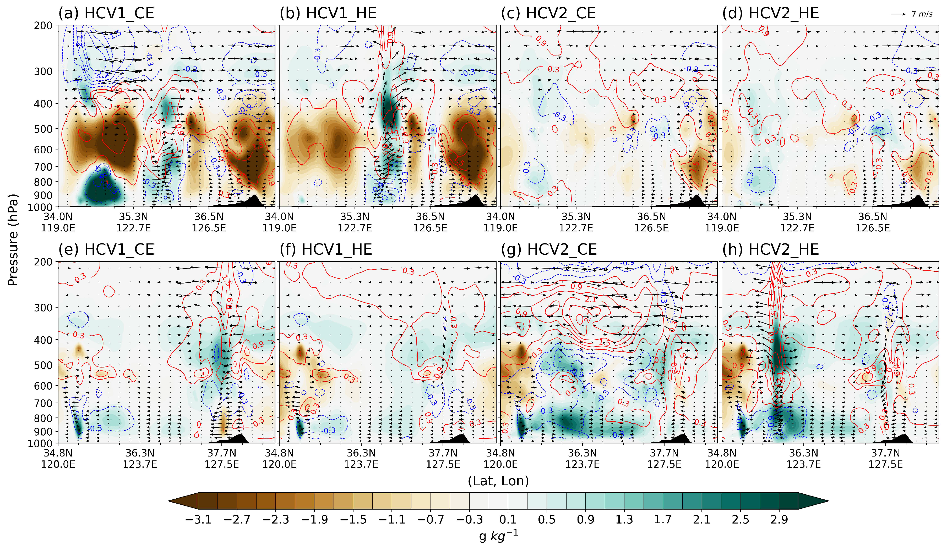
Figure 8 presents vertical cross-section differences along the A–B lines shown in Figure 6 and Figure 7 for Cases 1 and 2, respectively. In Case 1, within the convective area south of the Shandong Peninsula (near 121°E), the HCV1 experiments exhibited a drier mid-troposphere and increased humidity in the lower and upper troposphere compared to CONV (Figure 8a,b). In HCV1_CE, these moisture changes locally exceeded 3 g kg−1, while upper-level cooling near 250 hPa to the west exceeded 3 K. Furthermore, in both HCV1 experiments, a spurious convective signal appeared near 125°E accompanied by increased moisture, enhanced low- to mid-level convergence, and stronger vertical motion in the mid- to upper troposphere. This area also showed a temperature increase throughout most of the vertical column, except near the surface, likely due to latent heat release associated with the growth of solid-phase hydrometeors aloft. Conversely, cooling in the lower levels is likely attributable to erroneous precipitation generated by the misrepresented convective system.
In contrast, the HCV2 experiments exhibited smaller changes in moisture, temperature, and wind fields compared to HCV1 (Figure 8c,d). Around 34.5°N, corresponding to an actual convective cell location, a modest increase in WV—approximately 1 g kg−1—was evident throughout the column, with greater changes in HCV2_HE than in HCV2_CE. Upper-level warming of up to 1 K was also observed across a broader region, likely reflecting latent heat release associated with upper-level cloud development, as discussed later.
In Case 2, all experiments showed an overall increase in atmospheric moisture over the Yellow Sea, except in the mid-troposphere near 35°N and east of the Korean Peninsula. In contrast to Case 1, more pronounced changes in moisture and temperature were generally observed in the HCV2 experiments compared to HCV1 (Figure 8e–h). A clear signal of increased WV and upward motion was evident near 36°N (south of the Shandong Peninsula), particularly in HCV2_HE (Figure 8h), where strong upper-level divergence induced by convection was also observed. Regarding temperature, latent heat release and absorption associated with upper-level hydrometeor development and low-level precipitation were apparent. Notably, HCV2_CE exhibited stronger and more widespread upper-level warming than HCV2_HE, along with more marked enhancement of upper-level divergence relative to CONV. However, although HCV2_CE also showed overall moistening in the mid- and lower troposphere over the Yellow Sea, the magnitude and vertical extent of the convective structure were less pronounced than in HCV2_HE.
Figure 8.
Cross-sectional differences in WV mixing ratio (shading, g kg−1), temperature (contours, interval = 0.6 K), and wind vectors (m s−1) between CONV and (a,e) HCV1_CE, (b,f) HCV1_HE, (c,g) HCV2_CE, and (d,h) HCV2_HE at the final assimilation cycle. Panels (a–d) correspond to Case 1, and (e–h) to Case 2. Vertical velocity is multiplied by 3 for visualization clarity. The reference wind vector is shown in panel (d) and applies to all panels. Cross-section lines are indicated in Figure 6 and Figure 7.
3.3. Hydrometeor Distributions
Alongside changes in WV, temperature, and wind fields, the direct update of hydrometeors through ASR assimilation contributes to the development of system structures and, consequently, the evolution of forecast precipitation. To examine these impacts in relation to microphysical processes, changes in WV and individual hydrometeor species relative to CONV were analyzed at both the first and final cycling times (Figure 9). These profiles were computed by averaging over the primary convective regions (boxed areas in Figure 6 and Figure 7) for both Case 1 and Case 2.
In the first cycling step, key differences between HCV1 and HCV2 are observed as follows: HCV2 shows a significant decrease in WV near 600 hPa, accompanied by increases in both the upper (~350 hPa) and lower (~900 hPa) troposphere (Figure 9c,d). HCV1 exhibits a similar vertical distribution but with much smaller magnitudes, particularly near 600 hPa (Figure 9a,b). Furthermore, in HCV1, the most notable hydrometeor response was a reduction in cloud-phase hydrometeors near 600 hPa, with peak magnitudes of up to ~0.005 g kg−1, accompanied by a reduction in rainwater at the same level (~0.001 g kg−1). In contrast, HCV2 exhibited increases in most hydrometeor species, except for a slight decrease in cloud ice near 300 hPa. Solid-phase hydrometeors, in particular, show substantial increases in HCV2, with ice experiencing the most significant growth—peaking at approximately 0.003 g kg−1—while other species exhibit smaller increases (Figure 9c,d). The inclusion of solid-phase hydrometeors—key contributors to BT simulation—as CVs in HCV2 appears to increase degrees of freedom, potentially enabling larger WV increments.
Figure 9.
Vertical profiles of changes from CONV in the mixing ratios (g kg−1) of WV (black), cloud ice (blue), cloud water (green), snow (sky blue), graupel (purple), and rain (red) for (a,e) HCV1_CE, (b,f) HCV1_HE, (c,g) HCV2_CE, and (d,h) HCV2_HE. The upper panels (a–d) represent the first cycling step, and the lower panels (e–h) represent the final cycling step. All values are averaged over both cases and over the boxed regions indicated in Figure 6 and Figure 7.
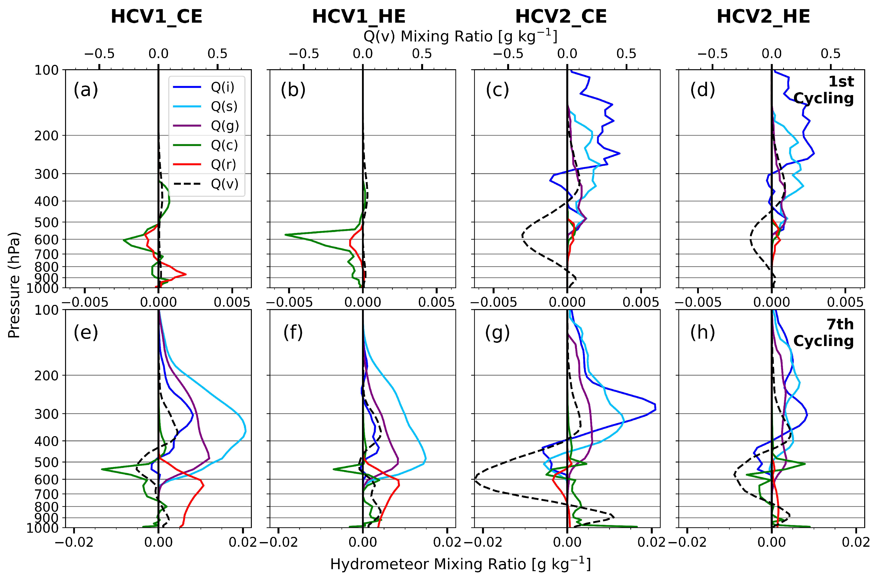
Since the averaged box area corresponds to a convectively active region with strong cloud impact, the CE approach tends to produce larger changes due to smaller observation errors. This contrasts with Figure 5, where averaged statistics cover the entire domain, including more clear-sky pixels. These effects are more pronounced under HCV2 settings, reflecting greater sensitivity to variations in solid-phase hydrometeors.
At the final cycling step, all four experiments exhibit a similar vertical pattern in WV changes—an increase at upper and lower levels and a decrease at mid-levels—although mid-level drying is less pronounced in HCV1_HE (Figure 9e–h). The upper-level solid-phase hydrometeors and lower-level rain produced in HCV1 appear to be associated with spurious convection over oceanic areas lacking real convection, as evidenced by the simulated BTs in Figure 6. In contrast, enhanced solid-phase hydrometeors in HCV2 correspond to localized convective cells at appropriate locations. They also align with widespread upper-level clouds characterized by low BTs (Figure 6e,f and Figure 7e,f), suggesting that more realistic updates can be achieved by directly initializing solid-phase hydrometeors. Additionally, peak growth altitudes of ice, snow, and graupel are higher in HCV2, whereas HCV1 tends to produce peaks at lower altitudes, reflecting shallower system development.
Within the same HCV2 configuration, differences in observation error specification are clearly reflected in the vertical profiles of HCV2_CE and HCV2_HE. As discussed earlier, CE assigns smaller observation errors in high-cloud-impact areas, resulting in larger cumulative increments in WV and hydrometeors. For example, HCV2_CE shows a marked increase in ice (~0.02 g kg−1) near 300 hPa, with snow and graupel peaking slightly below at approximately 0.014 and 0.006 g kg−1, respectively (Figure 9g). By comparison, HCV2_HE produces smaller peak increments of about 0.009, 0.007, and 0.004 g kg−1 for ice, snow, and graupel, respectively (Figure 9h). Furthermore, HCV2_CE exhibits the strongest mid-to-lower tropospheric drying among all experiments, with WV reductions exceeding −0.02 g kg−1 near 600 hPa. This pronounced drying likely impeded convection development south of the Shandong Peninsula at the final cycling time in Case 2, despite comparable upper-level cloud simulations (Figure 7e,f). In contrast, HCV2_HE shows more moderate drying (~−0.008 g kg−1), providing a more favorable background for simulating localized vertical convective development, consistent with Figure 8h.
To further examine how the different increments influenced the microphysical response and subsequent thermodynamic feedback, the 30 min net tendencies of WV and temperature were analyzed during the DA cycling period (Figure S3). Compared with HCV1, the HCV2 experiments exhibited more pronounced negative WV tendencies and positive temperature tendencies around 250 hPa during the first forecast period (Figure S3c,d). This tendency structure is physically consistent with enhanced cloud-ice deposition, likely associated with the increased upper-level WV and ice increments in the HCV2 experiments (Figure 9c,d). In this process, the assimilation-induced increases in upper-level WV and cloud ice promoted more active depositional ice growth, leading to reduced WV tendencies and latent heating aloft. This response also distinguished HCV2_CE from HCV2_HE, with HCV2_CE exhibiting stronger tendency signals around 250 hPa, consistent with the larger analyzed ice increments shown in Figure 9. Considering that HCV2_HE produced the smallest window-channel BT RMSE in the final-cycle analysis (Figure 5b), the more moderate tendency structure in HCV2_HE may indicate a more physically realistic adjustment during the assimilation cycle.
3.4. Forecast Verification of Hourly Accumulated Rainfall
To evaluate improvements in precipitation forecasts across the experiments, hourly rainfall from Domain 2 was verified against IMERG precipitation, which served as the reference. The RMSE and PC scores were analyzed to quantify the forecast performance.
In Case 1, the domain-averaged rainfall gradually increased with time, peaking around 2200 UTC on 25 July (Figure 10). RMSE in CONV showed an initial peak during the first 6 h of the forecast and another major peak near the maximum rainfall period, clearly indicating its failure to capture the heavy rainfall associated with the frontal system. The HCV1 experiments exhibited an initial increase in RMSE, followed by consistently smaller or comparable errors throughout most of the forecast period, except during the weakening stage (the last 8 h). The reduction in RMSE was greater in the CE configuration than in HE within the HCV1 experiments. In contrast, the HCV2 experiments did not show an initial increase in RMSE, though the subsequent error reduction was smaller than that of HCV1. However, HCV2_HE yielded the smallest RMSE near the peak rainfall time (~0.6 mm smaller than CONV), whereas HCV2_CE showed a similar error level to CONV at that time but a more rapid RMSE decrease afterward than any other experiment.
Figure 10.
Forecast scores of hourly rainfall for (a) RMSE and (b) PC in Case 1, obtained from CONV (black line), HCV1_CE (red dashed line), HCV1_HE (red solid line), HCV2_CE (blue dashed line), and HCV2_HE (blue solid line). Hourly accumulated rainfall from IMERG, averaged over D02, is shown with gray bars (right y-axis).
Similarly, the PC scores showed notable improvements in HCV2_HE, increasing by approximately 0.3 relative to CONV during the main rainfall period, whereas HCV2_CE showed no significant overall improvement. HCV1_HE displayed a delayed increase in PC of about 0.25 relative to CONV near 0400 UTC on 26 July. The more pronounced improvements in HCV2_HE during the peak rainfall period clearly demonstrate the potential benefits of assimilating ASR over upstream regions (in this case, the Yellow Sea), which allows for earlier and more accurate development of convective systems over the ocean. It is also noteworthy that, even when the HCV configuration includes all hydrometeor variables, forecast improvement may not be achieved if the observation error treatment does not adequately account for cloud effects during ASR assimilation.
In Case 2, the overall RMSE during the major rainfall period (the first 4 h of the forecast) was comparable to or slightly larger (by up to ~0.5 mm) than that of CONV across all ASR assimilation experiments (Figure 11). Compared with Case 1, Case 2 was characterized by substantially stronger convective activity and more intense low-level winds associated with the synoptic environment described in Section 2.5. Such conditions likely increased the nonlinearity of the convective system, potentially limiting the effectiveness of the current 3DVAR framework based on linear assumptions. In addition, the strong and localized convective structures produced larger initial O–B differences near the primary convective region, resulting in more frequent cloud-dependent QC rejections and reduced effective cloudy-radiance coverage during the cycling assimilation.
Figure 11.
Same as Figure 10, but for Case 2.
This issue may have been further amplified in the HCV1 experiments, where the absence of solid-phase hydrometeor updates likely required longer spin-up times for the development of ice-cloud structures. As a result, large O–B differences tended to persist throughout the cycling period, limiting moisture-field adjustments induced by ASR assimilation. This behavior was also evident in the number of assimilated AMI radiance observations (Figures S1 and S2). Unlike in Case 1, the HCV1 experiments in Case 2 assimilated fewer cloudy radiances than HCV2. This result suggests that persistently large O–B differences caused by the inadequate simulation of convective cloud structures in Case 2 reduced the effective cloudy-radiance coverage during cycling assimilation. Consequently, the impact of ASR assimilation on rainfall RMSE became less evident in Case 2. The RMSE increase was most pronounced in HCV2_CE, underscoring the importance of properly specifying scene-dependent observation errors for accurate rainfall forecasts.
Nevertheless, the PC score showed notable improvements in both HCV2 experiments, with HCV2_HE exhibiting the largest increase (+0.25 relative to CONV), while HCV2_CE improved by about +0.20. These results suggest that enhanced cloud representation, particularly through the inclusion of solid-phase hydrometeors, contributed positively to the spatial organization of precipitation within the multiscale frontal system. Conversely, the HCV1 experiments exhibited overall degradation in PC throughout the forecast period. The relative performance among the experiments was also generally consistent when verification was conducted using precipitation observations from surface AWSs over the Korean Peninsula.
To further examine the thermodynamic environment associated with the precipitation improvements, precipitable water (PW) fields during the onset of the peak rainfall period over the Korean Peninsula were compared against ERA5 (Figures S4 and S5). In both Cases 1 and 2, HCV2_HE most realistically reproduced the moist plume structure extending from the Yellow Sea toward the Korean Peninsula. Enhanced PW over the western Korean Peninsula and Yellow Sea region, associated with the observed heavy precipitation, was more clearly represented in the HCV2 experiments, particularly in HCV2_HE. The corresponding PC scores also showed the highest values in HCV2_HE (0.79 and 0.91 in Case 1 and Case 2, respectively), with overall improvements following the pattern HCV2 > HCV1 and HE > CE. The relatively limited precipitation improvement in the HCV1 experiments for Case 2 was also consistent with the PW verification results, which showed insufficient moisture enhancement and a weaker moist plume structure extending toward the Korean Peninsula (Figure S5c,d).
Consistent results were also obtained from radiosonde verification of temperature and dew-point temperature (Td) over the Korean Peninsula at similar observation times (Figure S6). For temperature, HCV2_HE performed comparably to or slightly better than CONV at most pressure levels, except near 850 hPa. More importantly, HCV2_HE showed the largest reduction in Td RMSE among all experiments, with an improvement of about 1 K relative to CONV in the 500–850 hPa layer, where AMI WV-channel radiances provide meaningful moisture information. These results further support that the improved moisture representation in HCV2_HE contributed to the enhanced precipitation forecasts.
4. Discussion
ASR observations from the WV channels of GK-2A AMI provide valuable information on the synoptic-scale moisture flow that governs the development of precipitation systems over East Asia. In ASR DA, accurately specifying observation errors in a scene-dependent manner is critical for properly accounting for cloud-related uncertainties. In addition, ASR assimilation enables simultaneous updates of both WV and cloud-related variables, which motivates extending prior approaches that limited CVs to only cloud water and rainwater (e.g., [27]). In particular, understanding the interaction between cloud-dependent observation error formulations and HCV configurations is an essential step toward improving the representation of moisture and hydrometeor fields and, ultimately, precipitation forecasts.
To address these issues, this study examined the impact of a cloud-dependent observation error model under different HCV configurations in the assimilation of GK-2A AMI all-sky WV radiances. Independent validation against observations further confirms that assimilating ASR with solid-phase hydrometeors included in the CV leads to more realistic representations of clouds and precipitating particles. In HCV1, solid-phase hydrometeors form only through model physical processes during integration, driven by updates to cloud water, rainwater, WV, and thermodynamic fields. As a result, cloud and precipitation structures associated with observed precipitating systems are less well reproduced within the DA cycling period than in HCV2.
The differences between HCV1 and HCV2 identified in this study may also be influenced by the model representation of ice-phase microphysical processes. Recent studies have shown that the representation of ice-phase microphysics in WDM6 can substantially influence the distribution of solid-phase hydrometeors and associated moisture structures. For example, ref. [62] demonstrated that introducing prognostic cloud ice number concentrations reduced excessive cloud ice amounts and improved precipitation and synoptic-scale environments in WDM6 simulations. These findings suggest that the hydrometeor sensitivity identified in the present study should be further examined using different microphysics configurations.
From the perspective of observation error treatment, the dynamic error model (HE) produces more moderate increments in regions with strong cloud influence, leading to better overall performance than the CE experiments. Although the quantitative differences in CMAX RMSE between HCV2_CE and HCV2_HE are relatively small, WV-channel ASR assimilation primarily affects upper-tropospheric cloud and ice-phase hydrometeor structures associated with deep convection. Therefore, improvements associated with the dynamic observation error treatment are more clearly reflected in upper-level cloud organization, moisture structure, and spatial convective coherence than in CMAX-based verification metrics alone. This behavior is also evident in the cross-sectional analysis (Figure 8) and the ERA5/radiosonde verification (Figures S4–S6), where HCV2_HE more realistically reproduces the upper-level moisture, temperature, and circulation structures associated with the observed convective system propagating from the Yellow Sea toward the Korean Peninsula. Correspondingly, HCV2_HE also showed the most robust improvement in precipitation forecasts. These results highlight the benefit of updating all hydrometeor species via ASR assimilation (HCV2 > HCV1) and underscore the importance of a dynamic observation error model for achieving physically consistent analyses and forecast improvements, particularly when solid-phase hydrometeors are included in the HCV (HE > CE under HCV2).
Despite these improvements, several aspects warrant further investigation. First, background error covariances for hydrometeors should be re-estimated rather than relying on the constant values used in this study. The specification of hydrometeor background error covariances may influence the magnitude and vertical structure of the analysis increments and partly contribute to the negative cloud-top BT biases associated with excessive upper-level ice-phase hydrometeors in the HCV2 experiments. Uncertainties in hydrometeor background error covariances may interact with systematic microphysics biases during model integration, potentially amplifying upper-level hydrometeor biases. Future adoption of flow-dependent background error covariances, such as ensemble-based covariances, may help alleviate this problem and also improve the structure of analysis increments for solid-phase hydrometeors, thereby complementing the HE framework used in this study.
Nevertheless, the improved moisture structures, more realistic convective organization, and improved precipitation forecasts suggest that the HCV2_HE improvements identified in this study retain physical consistency even under the simplified hydrometeor covariance specification used here. Second, the sensitivity of the results to different microphysics schemes and cloud treatments in the RTM should be examined, particularly to address persistent cold biases near cloud edges in simulated BTs. Finally, because this study examined only two convective cases, the statistical robustness of the present conclusions remains limited. Future work should further evaluate the general applicability of the full HCV (HCV2) and HE approaches under a broader range of weather conditions, including stratiform precipitation and tropical cyclones. Extending this evaluation beyond the current 3DVAR context to ensemble-based DA frameworks also represents an important direction for future research. Such frameworks may also provide flow-dependent estimates of forecast error, enabling a more rigorous partitioning of innovation variance into forecast and observation error components and helping address the additional uncertainty associated with using O–B STD directly as a proxy for observation error.
5. Conclusions
In this study, the impacts of cloud-dependent observation errors and HCV configurations were investigated through the assimilation of all-sky WV radiances from the GK-2A AMI. A fifth-order polynomial observation error model was constructed as a function of the cloud impact parameter and evaluated against the conventional constant-error assumption. Four ASR experiments were designed by combining two observation error treatments—CE and HE—with two HCV configurations: HCV1, which excludes solid-phase hydrometeors, and HCV2, which includes all hydrometeor species. This experimental design enabled a systematic assessment of both the observation error representation and the role of solid-phase hydrometeors. In addition, ASR-based experiments were compared with a control experiment that assimilated only conventional observations.
The main findings and conclusions are summarized as follows:
- (1)
- When assimilating ASR, directly updating solid-phase hydrometeors by including them in the CV not only enables a more accurate representation of cloud distribution but also improves the depiction of developing precipitation systems;
- (2)
- However, improvements from the HCV2 configuration alone are not guaranteed, and these benefits are more consistently realized when HE is applied;
- (3)
- This additional improvement from applying HE arises from accounting for increased uncertainties in cloud-affected regions, which can strongly influence the development of convective structures.
Supplementary Materials
The following supporting information can be downloaded at: https://www.mdpi.com/article/10.3390/rs18132246/s1, Figure S1: Time series of the total number of assimilated AMI WV-channel radiances during the cycling assimilation period for Case 1 after the application of the cloud-dependent quality control. HCV1_CE (red), HCV1_HE (orange), HCV2_CE (sky blue), and HCV2_HE (blue). The y-axis is truncated to emphasize inter-experiment differences; Figure S2: Same as Figure S1, but for Case 2; Figure S3: Vertical profiles of net tendencies of temperature (red lines; K h−1) and WV mixing ratio (blue lines; g kg−1 h−1) in panels (a–d). Tendencies are calculated from the first 30-min forecast after the initial DA cycle, spatially averaged over the boxed regions indicated in Figure 6 and Figure 7, and then averaged over both Case 1 and Case 2. Panels (a), (b), (c), and (d) correspond to HCV1_CE, HCV1_HE, HCV2_CE, and HCV2_HE, respectively; Figure S4: Precipitable water (shading; mm) and 500 hPa geopotential height (contours; gpm; 30 gpm interval) for Case 1 at 1800 UTC 25 July 2019 (15-h forecast). Panel (a) shows ERA5, while panels (b)–(f) show CONV, HCV1_CE, HCV1_HE, HCV2_CE, and HCV2_HE, respectively. The PCORR score shown in each panel represents the pattern correlation of precipitable water over Domain 2 after regridding the WRF fields to the ERA5 grid; Figure S5: Same as Figure S4, but for Case 2 at 0300 UTC 3 August 2020 (3-h forecast); Figure S6: RMSE profiles of (a) temperature (K) and (b) dew-point temperature (K) verified against radiosonde observations over the Korean Peninsula for CONV (black line), HCV1_CE (red dashed line), HCV1_HE (red solid line), HCV2_CE (blue dashed line), and HCV2_HE (blue solid line). Errors were averaged over Case 1 and Case 2 near the peak rainfall period over the Korean Peninsula (Case 1 at 1800 UTC 25 July 2019 and Case 2 at 0000 UTC 3 August 2020). The right y-axis indicates the number of radiosonde observations used for verification at each pressure level.
Author Contributions
Conceptualization, S.-Y.J. and K.-H.M.; methodology, S.-Y.J. and K.-H.M.; software, S.-Y.J.; validation, S.-Y.J.; formal analysis, S.-Y.J. and K.-H.M.; investigation, S.-Y.J.; resources, K.-H.M.; data curation, S.-Y.J.; writing—original draft preparation, S.-Y.J.; writing—review and editing, S.-Y.J. and K.-H.M.; visualization, S.-Y.J.; supervision, K.-H.M.; project administration, K.-H.M.; funding acquisition, K.-H.M. All authors have read and agreed to the published version of the manuscript.
Funding
This work is supported by the Korea Meteorological Administration Research and Development Program under Grant KMI2022-00310 and by the National Research Foundation of Korea (NRF) grant funded by the Korea government (MSIT) (RS-2025-02242970).
Data Availability Statement
The model output data generated in this study are available from the corresponding author upon reasonable request due to their large size. The assimilated and validation datasets, including the GK-2A AMI Level 1B satellite data, are available via the Korea Meteorological Administration (KMA) API Hub (https://apihub.kma.go.kr/, accessed on 2 August 2023), subject to KMA data access policies. The IMERG precipitation data are publicly available at https://gpm.nasa.gov/data (accessed on 9 September 2024). The NCEP GDAS/FNL 0.25° global analysis and forecast data used for the initial and boundary conditions are publicly available at https://gdex.ucar.edu/datasets/d083003/ (accessed on 4 June 2024). The ERA5 pressure-level reanalysis data used for thermodynamic-field verification are available at https://cds.climate.copernicus.eu/datasets/reanalysis-era5-pressure-levels (accessed on 4 October 2025).
Acknowledgments
The authors acknowledge support from the Brain Korea 21 program through a research scholarship.
Conflicts of Interest
The authors declare no conflicts of interest.
Correction Statement
This article has been republished with a minor correction to the image quality of all figures. This change does not affect the scientific content of the article.
Abbreviations
The following abbreviations are used in this manuscript:
| ASR | All-sky radiance |
| HCV | Hydrometeor control variable |
| BT | Brightness temperature |
| CSR | Clear-sky radiance |
| RTM | Radiative transfer model |
| STD | Standard deviation |
| FG | First-guess |
| O-B | Observation-minus-background |
| QC | Quality control |
| WV | Water vapor |
| GK-2A | Geostationary Korea Multi-Purpose Satellite-2A |
| AMI | Advanced Meteorological Imager |
| DA | Data assimilation |
| CV | Control variable |
| WRF | Weather Research and Forecasting |
| 3DVAR | Three-dimensional variational |
| CRTM | Community Radiative Transfer Model |
| JCSDA | Joint Center for Satellite Data Assimilation |
| COMS-1 | Communication, Ocean, and Meteorological Satellite |
| IR | Infrared |
| AHI | Advanced Himawari Imager |
| ABI | Advanced Baseline Imager |
| GOES-16 | Geostationary Operational Environmental Satellite-16 |
| AMV | Atmospheric motion vector |
| AWS | Automatic weather stations |
| ASOS | Automated synoptic observing system |
| CAPPI | Constant altitude plan position indicator |
| PPI | Plan position indicator |
| IMERG | Integrated Multi-satellitE Retrievals for GPM |
| HE | Higher-order regressed error |
| CE | Constant error |
| BC | Bias Correction |
| VarBC | Variational BC |
| RMSE | Root mean square error |
| PC | Pattern correlation |
| FSS | Fraction skill score |
| CMAX | Column-maximum radar reflectivity |
| PW | Precipitable Water |
| Td | Dew-point Temperature |
References
- Talagrand, O. Assimilation of observations, an introduction. J. Meteorol. Soc. Jpn. Ser. II 1997, 75, 191–209. [Google Scholar] [CrossRef] [Scilit] [PubMed]
- Kalnay, E. Atmospheric Modeling, Data Assimilation and Predictability; Cambridge University Press: Cambridge, UK, 2003; 341p. [Google Scholar]
- Bauer, P.; Thorpe, A.; Brunet, G. The quiet revolution of numerical weather prediction. Nature 2015, 525, 47–55. [Google Scholar] [CrossRef] [Scilit] [PubMed]
- Carrassi, A.; Bocquet, M.; Bertino, L.; Evensen, G. Data assimilation in the geosciences: An overview of methods, issues, and perspectives. WIREs Clim. Change 2018, 9, e535. [Google Scholar] [CrossRef] [Scilit]
- Zhu, Y.; Gelaro, R. Observation sensitivity calculations using the adjoint of the Gridpoint Statistical Interpolation (GSI) analysis system. Mon. Weather Rev. 2008, 136, 335–351. [Google Scholar] [CrossRef] [Scilit]
- Peubey, C.; McNally, A.P. Characterization of the impact of geostationary clear-sky radiances on wind analyses in a 4D-Var context. Q. J. R. Meteorol. Soc. 2009, 135, 1863–1876. [Google Scholar] [CrossRef] [Scilit]
- Bormann, N.; Geer, A.J.; Bauer, P. Estimates of observation-error characteristics in clear and cloudy regions for microwave imager radiances from numerical weather prediction. Q. J. R. Meteorol. Soc. 2011, 137, 2014–2023. [Google Scholar] [CrossRef] [Scilit]
- Honda, T.; Miyoshi, T.; Lien, G.; Nishizawa, S.; Yoshida, R.; Adachi, S.A.; Terasaki, K.; Okamoto, K.; Tomita, H.; Bessho, K. Assimilating all-sky Himawari-8 satellite infrared radiances: A case of Typhoon Soudelor (2015). Mon. Weather Rev. 2018, 146, 213–229. [Google Scholar] [CrossRef] [Scilit]
- Minamide, M.; Zhang, F. Assimilation of all-sky infrared radiances from Himawari-8 and impacts of moisture and hydrometeor initialization on convection-permitting tropical cyclone prediction. Mon. Weather Rev. 2018, 146, 3241–3258. [Google Scholar] [CrossRef] [Scilit]
- Okamoto, K.; Sawada, Y.; Kunii, M. Comparison of assimilating all-sky and clear-sky infrared radiances from Himawari-8 in a mesoscale system. Q. J. R. Meteorol. Soc. 2019, 145, 745–766. [Google Scholar] [CrossRef] [Scilit]
- Xian, Z.; Chen, K.; Zhu, J. All-sky assimilation of the MWHS-2 observations and evaluation of the impacts on the analyses and forecasts of binary typhoons. J. Geophys. Res. Atmos. 2019, 124, 6359–6378. [Google Scholar] [CrossRef] [Scilit]
- Xu, D.; Liu, Z.; Fan, S.; Chen, M.; Shen, F. Assimilating all-sky infrared radiances from Himawari-8 using the 3DVar method for the prediction of a severe storm over North China. Adv. Atmos. Sci. 2021, 38, 661–676. [Google Scholar] [CrossRef] [Scilit]
- Duncan, D.; Bormann, N.; Geer, A.J.; Weston, P. Assimilation of AMSU-A in all-sky conditions. Mon. Weather Rev. 2022, 150, 1023–1041. [Google Scholar] [CrossRef] [Scilit]
- Johnson, A.; Wang, X.; Jones, T. Impacts of assimilating GOES-16 ABI channels 9 and 10 clear air and cloudy radiance observations with additive inflation and adaptive observation error in GSI-EnKF for a case of rapidly evolving severe supercells. J. Geophys. Res. Atmos. 2022, 127, e2021JD036157. [Google Scholar] [CrossRef] [Scilit]
- Degelia, S.K.; Wang, X.; Wang, Y.; Johnson, A. Assimilation of GOES-16 ABI all-sky radiance observations in RRFS using EnVar: Methodology, system development, and impacts for a severe convective event. Mon. Weather Rev. 2023, 151, 2739–2758. [Google Scholar] [CrossRef] [Scilit]
- Zhu, L.; Xue, M.; Kong, R.; Min, J. Direct assimilation of all-sky GOES-R ABI radiances in GSI EnKF for the analysis and forecasting of a mesoscale convective system. Mon. Weather Rev. 2023, 151, 737–760. [Google Scholar] [CrossRef] [Scilit]
- Geer, A.J. Correlated observation error models for assimilating all-sky infrared radiances. Atmos. Meas. Tech. 2019, 12, 3629–3657. [Google Scholar] [CrossRef] [Scilit]
- Harnisch, F.; Weissmann, M.; Periáñez, Á. Error model for the assimilation of cloud-affected infrared satellite observations in an ensemble data assimilation system. Q. J. R. Meteorol. Soc. 2016, 142, 1797–1808. [Google Scholar] [CrossRef] [Scilit]
- Zou, X.; Zhuge, X.; Weng, F. Characterization of bias of Advanced Himawari Imager infrared observations from NWP background simulations using CRTM and RTTOV. J. Atmos. Ocean. Technol. 2016, 33, 2553–2567. [Google Scholar] [CrossRef] [Scilit]
- Zhuge, X.; Zou, X.; Wang, Y. A comparison between three surface type data sets adopted by the Community Radiative Transfer Model. Remote Sens. Lett. 2017, 8, 801–810. [Google Scholar] [CrossRef] [Scilit]
- Li, J.; Geer, A.; Okamoto, K.; Otkin, J.; Liu, Z.Q.; Han, W.; Wang, P. Satellite all-sky infrared radiance assimilation: Recent progress and future perspectives. Adv. Atmos. Sci. 2022, 39, 9–21. [Google Scholar] [CrossRef] [Scilit]
- Xu, D.; Zhang, X.; Liu, Z.; Shen, F. All-sky infrared radiance data assimilation of FY-4A AGRI with different physical parameterizations for the prediction of an extremely heavy rainfall event. Atmos. Res. 2023, 293, 106898. [Google Scholar] [CrossRef] [Scilit]
- Wu, Y.; Qin, Z.; Li, J.; Bai, X. Primary impact evaluation of surface temperature observations for microwave temperature sounding data assimilation over land. Remote Sens. 2024, 16, 395. [Google Scholar] [CrossRef] [Scilit]
- Qin, L.; Chen, Y.; Meng, D.; Cheng, X.; Zhang, P. Variational all-sky assimilation framework for MWHS-II with hydrometeors control variables and its impacts on analysis and forecast of typhoon cases. J. Adv. Model. Earth Syst. 2024, 16, e2023MS004153. [Google Scholar] [CrossRef] [Scilit]
- Geer, A.J.; Bauer, P. Observation errors in all-sky data assimilation. Q. J. R. Meteorol. Soc. 2011, 137, 2024–2037. [Google Scholar] [CrossRef] [Scilit]
- Okamoto, K.; McNally, A.P.; Bell, W. Progress towards the assimilation of all-sky infrared radiances: An evaluation of cloud effects. Q. J. R. Meteorol. Soc. 2014, 140, 1603–1614. [Google Scholar] [CrossRef] [Scilit]
- Hastuti, M.I.; Min, K.-H. Impact of assimilating GK-2A all-sky radiance with a new observation error for summer precipitation forecasting. Remote Sens. 2023, 15, 3113. [Google Scholar] [CrossRef] [Scilit]
- Lorenc, A.C.; Ballard, S.P.; Bell, R.S.; Ingleby, N.B.; Andrews, P.L.F.; Barker, D.M.; Bray, J.R.; Clayton, A.M.; Dalby, T.; Li, D.; et al. The Met Office global three-dimensional variational data assimilation scheme. Q. J. R. Meteorol. Soc. 2000, 126, 2991–3012. [Google Scholar] [CrossRef]
- Ingleby, N.B. The statistical structure of forecast errors and its representation in the Met Office global 3-D variational data assimilation scheme. Q. J. R. Meteorol. Soc. 2001, 127, 209–231. [Google Scholar] [CrossRef]
- Zupanski, M.; Zupanski, D.; Vukicevic, T.; Eis, K.; Haar, T.V. CIRA/CSU four-dimensional variational data assimilation system. Mon. Weather Rev. 2005, 133, 829–843. [Google Scholar] [CrossRef] [Scilit]
- Huang, X.; Xiao, Q.; Barker, D.M.; Zhang, X.; Michalakes, J.; Huang, W.; Henderson, T.; Bray, J.; Chen, Y.; Ma, Z.; et al. Four-dimensional variational data assimilation for WRF: Formulation and preliminary results. Mon. Weather Rev. 2009, 137, 299–314. [Google Scholar] [CrossRef] [Scilit]
- Li, X.; Zou, X.; Zeng, M.; Zhuge, X.; Wang, N. Characteristic differences of CrIS all-sky simulations of brightness temperature with different microphysics parameterization schemes. Mon. Weather Rev. 2022, 150, 2629–2657. [Google Scholar] [CrossRef] [Scilit]
- Shen, F.; Song, L.; He, Z.; Xu, D.; Chen, J.; Huang, L. Impacts of adding hydrometeor control variables on the radar reflectivity data assimilation for the 6–8 August 2018 mesoscale convective system case. Atmos. Res. 2023, 295, 107012. [Google Scholar] [CrossRef] [Scilit]
- Yang, S.; Li, D.; Duan, Y.; Chen, Y.; Liu, Z.; Huang, X.-Y. Assimilating precipitation data via full-hydrometeor scheme in WRF 4D-Var for convective precipitation forecast associated with the Northeast China cold vortex (NCCV). J. Geophys. Res. Atmos. 2025, 130, e2024JD042427. [Google Scholar] [CrossRef] [Scilit]
- Skamarock, W.C.; Klemp, J.B.; Dudhia, J.; Gill, D.O.; Liu, Z.; Berner, J.; Wang, W.; Powers, J.G.; Duda, M.G.; Barker, D.M.; et al. A Description of the Advanced Research WRF Model Version 4.1; National Center for Atmospheric Research: Boulder, CO, USA, 2019. [Google Scholar] [CrossRef]
- Lim, K.-S.; Hong, S.-Y. Development of an effective double-moment cloud microphysics scheme with prognostic cloud condensation nuclei (CCN) for weather and climate models. Mon. Weather Rev. 2010, 138, 1587–1612. [Google Scholar] [CrossRef] [Scilit]
- Mlawer, E.J.; Taubman, S.J.; Brown, P.D.; Iacono, M.J.; Clough, S.A. Radiative transfer for inhomogeneous atmospheres: RRTM, a validated correlated-k model for the longwave. J. Geophys. Res. 1997, 102, 16663–16682. [Google Scholar] [CrossRef] [Scilit]
- Dudhia, J. Numerical study of convection observed during the Winter Monsoon Experiment using a mesoscale two-dimensional model. J. Atmos. Sci. 1989, 46, 3077–3107. [Google Scholar] [CrossRef] [Scilit]
- Zheng, Y.; Alapaty, K.; Herwehe, J.A.; Del Genio, A.D.; Niyogi, D. Improving high-resolution weather forecasts using the Weather Research and Forecasting (WRF) Model with an updated Kain–Fritsch scheme. Mon. Weather Rev. 2016, 144, 833–860. [Google Scholar] [CrossRef] [Scilit]
- Jiménez, P.A.; Dudhia, J.; González-Rouco, J.F.; Navarro, J.; Montávez, J.P.; García-Bustamante, E. A revised scheme for the WRF surface layer formulation. Mon. Weather Rev. 2012, 140, 898–918. [Google Scholar] [CrossRef] [Scilit]
- Tewari, M.; Chen, F.; Wang, W.; Dudhia, J. Implementation and verification of the unified Noah land surface model in the WRF Model. In Proceedings of the 20th Conference on Weather Analysis and Forecasting/16th Conference on Numerical Weather Prediction, Seattle, WA, USA; American Meteorological Society: Boston, MA, USA, 2004; Available online: https://ams.confex.com/ams/84Annual/techprogram/paper_69061.htm (accessed on 2 April 2023).
- Hong, S.-Y.; Noh, Y.; Dudhia, J. A new vertical diffusion package with an explicit treatment of entrainment processes. Mon. Weather Rev. 2006, 134, 2318–2341. [Google Scholar] [CrossRef] [Scilit]
- National Centers for Environmental Prediction; National Weather Service; NOAA; U.S. Department of Commerce. NCEP GDAS/FNL 0.25° Global Tropospheric Analyses and Forecast Grids; Research Data Archive at the National Center for Atmospheric Research, Computational and Information Systems Laboratory; NCEP: College Park, MD, USA, 2015. [Google Scholar] [CrossRef] [Scilit]
- Barker, D.M.; Huang, W.; Guo, Y.; Bourgeois, A.J.; Xiao, Q.N. A three-dimensional variational data assimilation system for MM5: Implementation and initial results. Mon. Weather Rev. 2004, 132, 897–914. [Google Scholar] [CrossRef] [Scilit]
- Barker, D.M.; Huang, X.; Liu, Z.; Auligné, T.; Zhang, X.; Rugg, S.; Ajjaji, R.; Bourgeois, A.; Bray, J.; Chen, Y.; et al. The Weather Research and Forecasting Model’s community variational/ensemble data assimilation system: WRFDA. Bull. Am. Meteorol. Soc. 2012, 93, 831–843. [Google Scholar] [CrossRef] [Scilit]
- Han, Y.; Delst, V.P.; Liu, Q.; Weng, F.; Yan, B.; Treadon, R.; Derber, J. JCSDA Community Radiative Transfer Model (CRTM)—Version 1; NOAA Technical Report; NESDIS: Silver Spring, MD, USA, 2006. [Google Scholar]
- National Institute of Meteorological Research. Improvement of Performance in Very-Short-Range Forecast Models with Nowcasting Data; National Institute of Meteorological Research: Seogwipo-si, Republic of Korea, 2011; 227p. (In Korean) [Google Scholar]
- Min, K.-H.; Choo, S.-H.; Lee, D.-H.; Lee, G.-W. Evaluation of WRF cloud microphysics schemes using radar observations. Weather Forecast. 2015, 30, 1571–1589. [Google Scholar] [CrossRef] [Scilit]
- Weather Radar Center. Development of Optimized Techniques for Dual-Polarization Radar Harmonization; Weather Radar Center: Seoul, Republic of Korea, 2017; 243p. (In Korean) [Google Scholar]
- Huffman, G.J.; Stocker, E.F.; Bolvin, D.T.; Nelkin, E.J.; Tan, J. GPM IMERG Final Precipitation L3 Half Hourly 0.1° × 0.1° V07; Goddard Earth Sciences Data and Information Services Center (GES DISC): Greenbelt, MD, USA, 2023. [Google Scholar] [CrossRef]
- Hersbach, H.; Bell, B.; Berrisford, P.; Biavati, G.; Horányi, A.; Muñoz Sabater, J.; Nicolas, J.; Peubey, C.; Radu, R.; Rozum, I.; et al. ERA5 Hourly Data on Pressure Levels from 1940 to Present; Copernicus Climate Change Service (C3S) Climate Data Store (CDS): Reading, UK, 2023. [Google Scholar] [CrossRef]
- Parrish, D.F.; Derber, J.C. The National Meteorological Center’s spectral statistical-interpolation analysis system. Mon. Weather Rev. 1992, 120, 1747–1763. [Google Scholar] [CrossRef] [Scilit]
- Lee, J.-W.; Min, K.-H.; Lee, Y.-H.; Lee, G.-W. X-Net-based radar data assimilation study over the Seoul metropolitan area. Remote Sens. 2020, 12, 893. [Google Scholar] [CrossRef] [Scilit]
- Feng, C.; Pu, Z. A bias correction scheme with the symmetric cloud proxy variable and its influence on assimilating all-sky GOES-16 brightness temperatures. Mon. Weather Rev. 2022, 150, 3305–3323. [Google Scholar] [CrossRef] [Scilit]
- Derber, J.C.; Wu, W. The use of TOVS cloud-cleared radiances in the NCEP SSI analysis system. Mon. Weather Rev. 1998, 126, 2287–2299. [Google Scholar] [CrossRef] [Scilit]
- Dee, D.P. Variational bias correction of radiance data in the ECMWF system. In Proceedings of the ECMWF Workshop on Assimilation of High Spectral Resolution Sounders in NWP, Shinfield Park, Reading, UK, 28 June–1 July 2004; ECMWF: Reading, UK, 2004; pp. 97–112. Available online: https://www.ecmwf.int/sites/default/files/elibrary/2004/8930-variational-bias-correction-radiance-data-ecmwf-system.pdf (accessed on 12 July 2024).
- Okamoto, K. Evaluation of IR radiance simulation for all-sky assimilation of Himawari-8/AHI in a mesoscale NWP system. Q. J. R. Meteorol. Soc. 2017, 143, 1517–1527. [Google Scholar] [CrossRef] [Scilit]
- Bae, J.-H.; Min, K.-H. Forecast characteristics of radar data assimilation based on the scales of precipitation systems. Remote Sens. 2022, 14, 605. [Google Scholar] [CrossRef] [Scilit]
- Hastuti, M.I.; Min, K.-H.; Lee, J.-W. Improving radar data assimilation forecast using advanced remote sensing data. Remote Sens. 2023, 15, 2760. [Google Scholar] [CrossRef] [Scilit]
- Zhang, Y.; Clothiaux, E.E.; Stensrud, D.J. Correlation structures between satellite all-sky infrared brightness temperatures and the atmospheric state at storm scales. Adv. Atmos. Sci. 2022, 39, 714–732. [Google Scholar] [CrossRef] [Scilit]
- Song, H.-J.; Sohn, B.-J. An evaluation of WRF microphysics schemes for simulating the warm-type heavy rain over the Korean Peninsula. Asia-Pac. J. Atmos. Sci. 2018, 54, 225–236. [Google Scholar] [CrossRef] [Scilit]
- Park, S.-Y.; Lim, K.-S. Implementation of prognostic cloud ice number concentrations for the Weather Research and Forecasting (WRF) Double-Moment 6-class (WDM6) microphysics scheme. J. Adv. Model. Earth Syst. 2023, 15, e2022MS003009. [Google Scholar] [CrossRef] [Scilit]
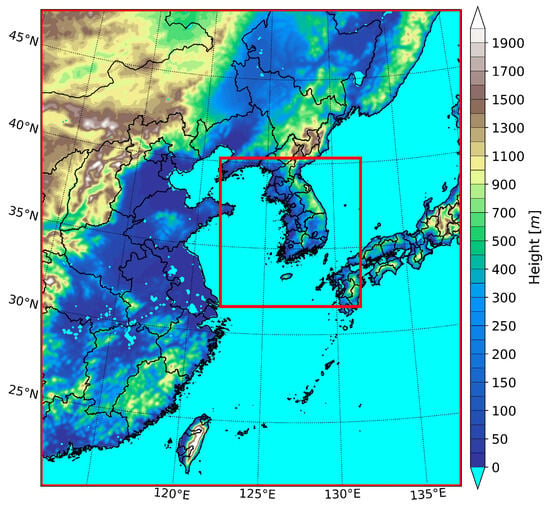
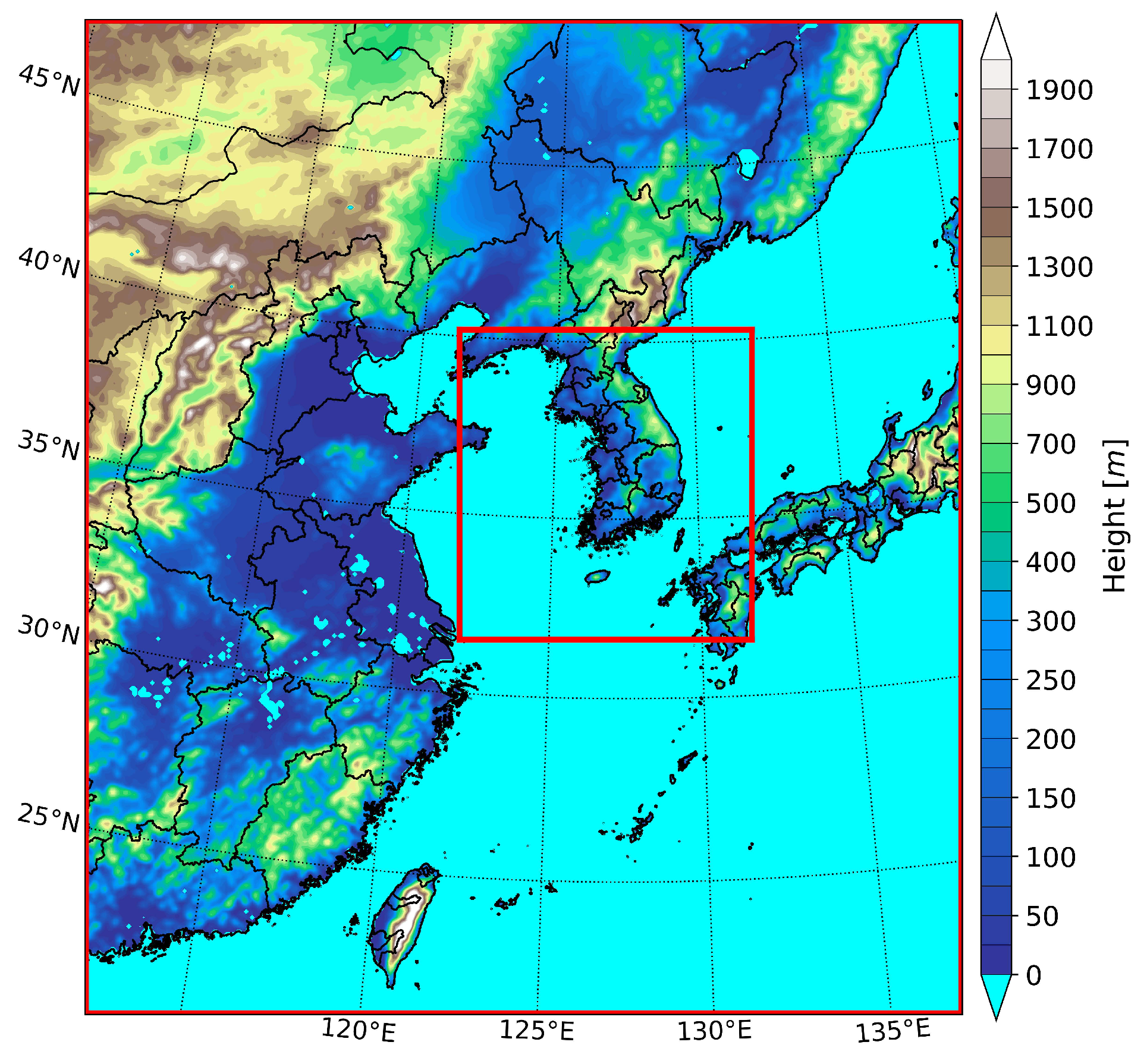
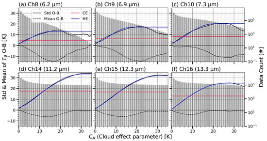
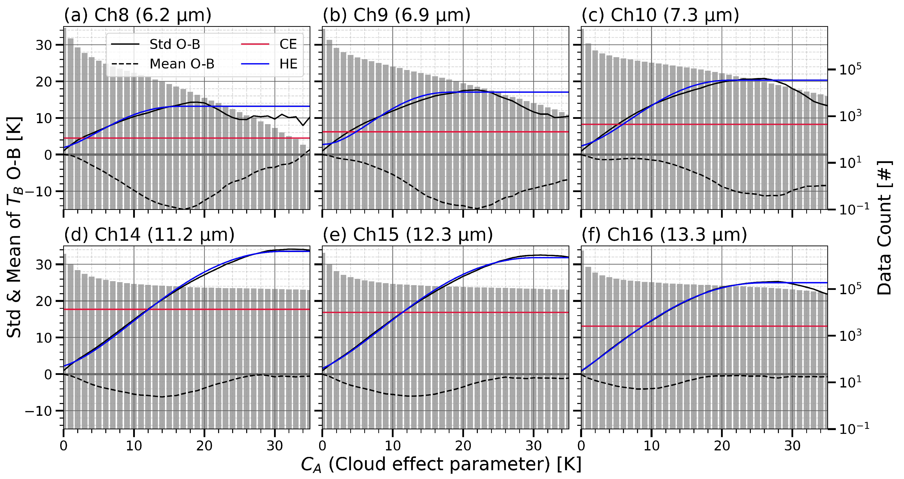
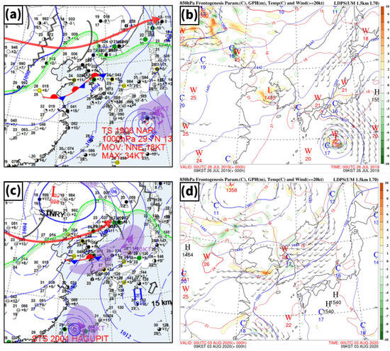
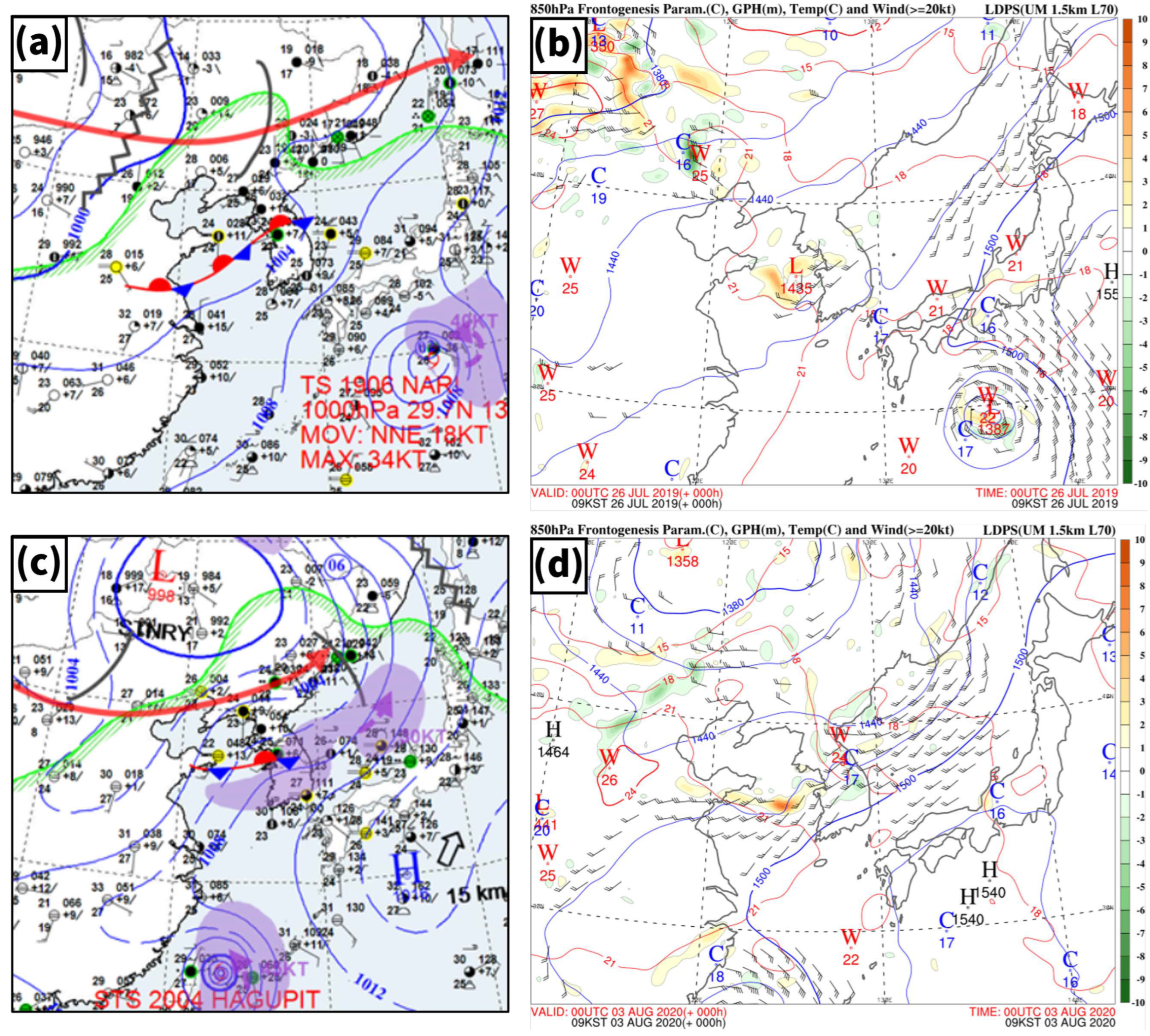
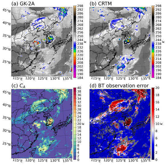
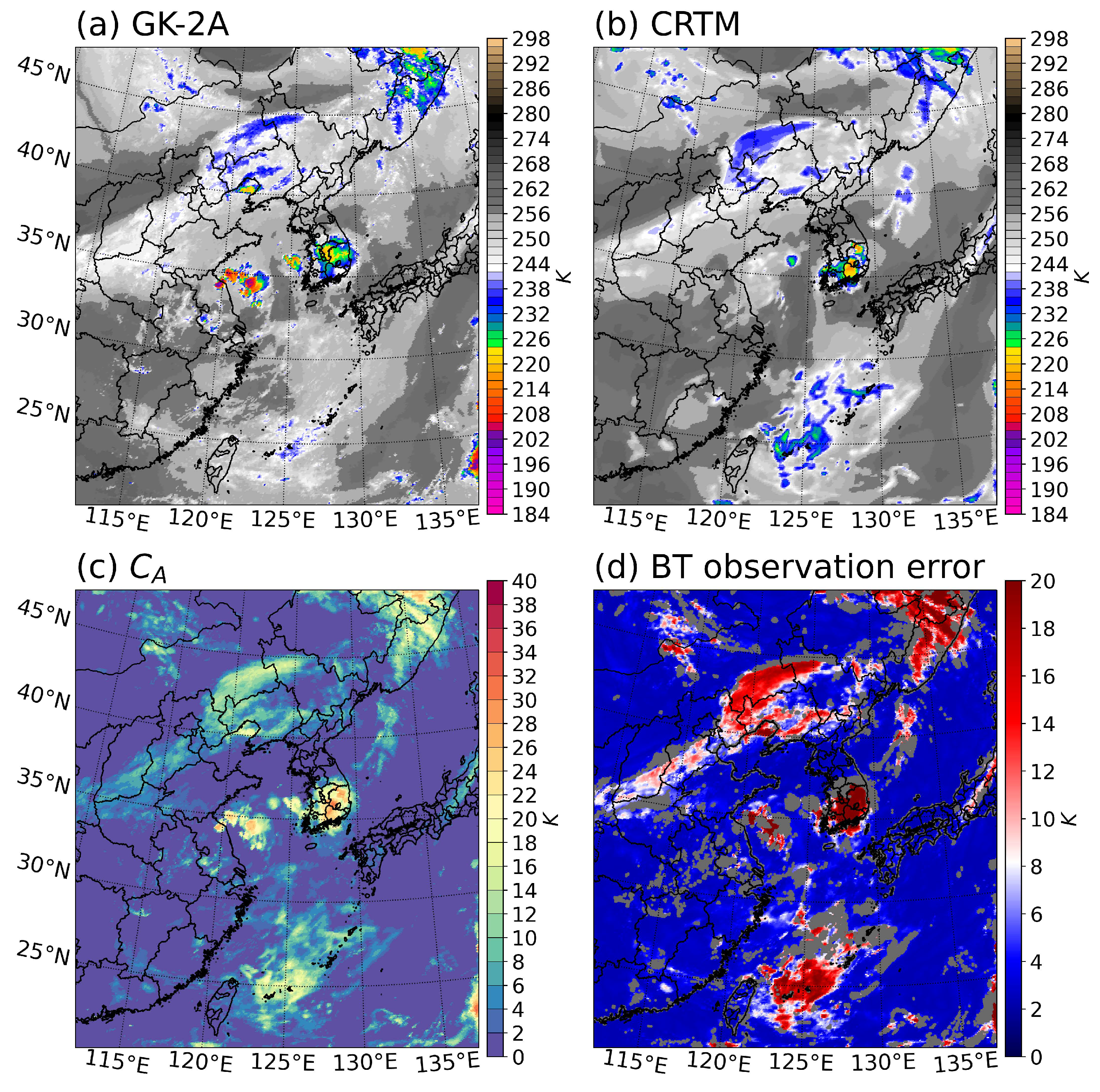
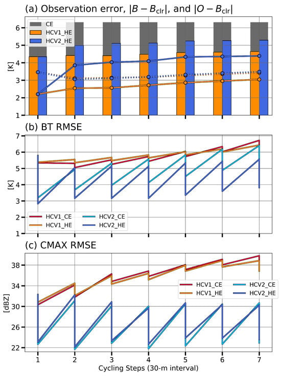
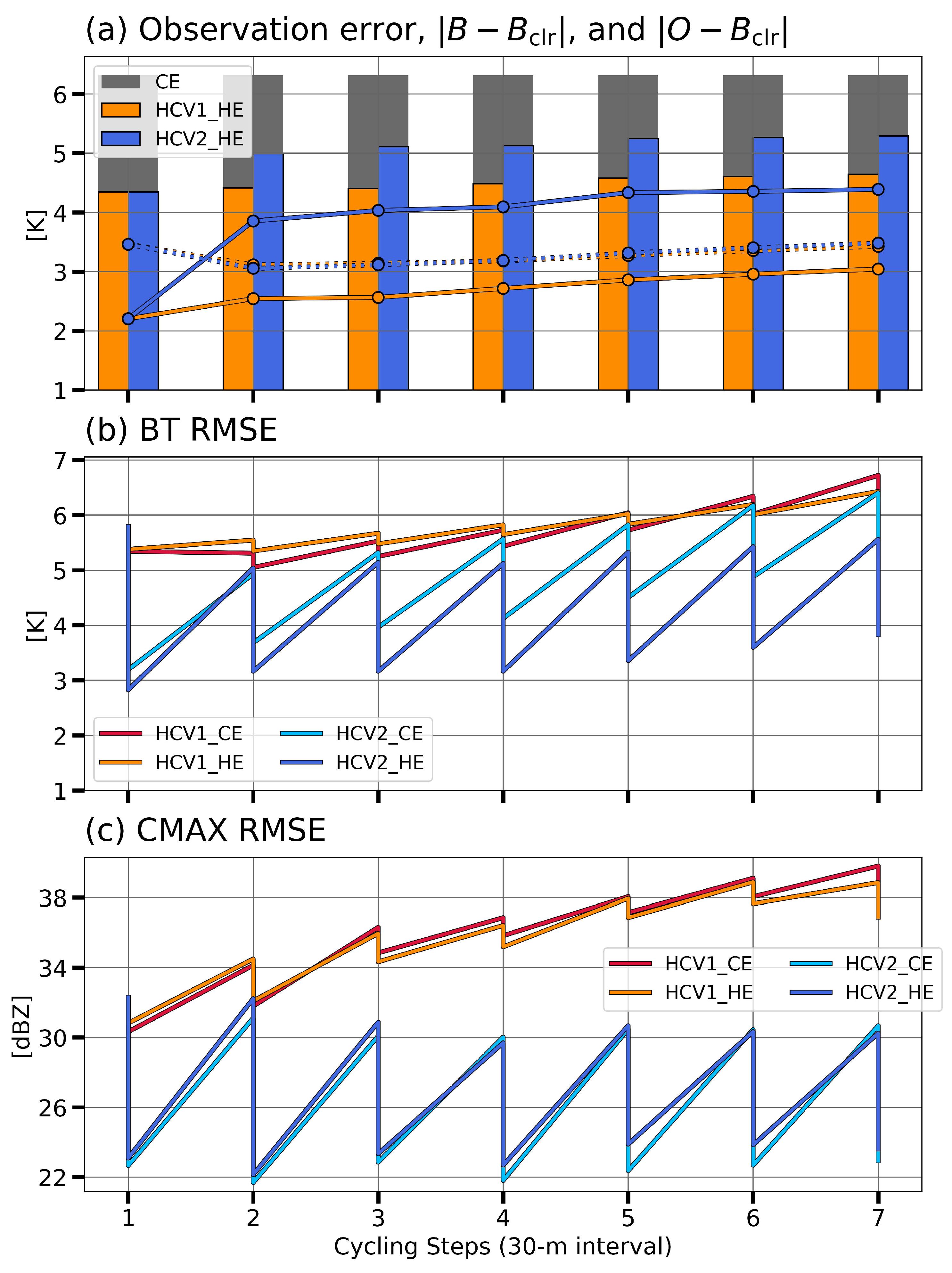
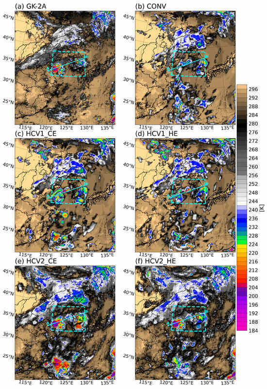
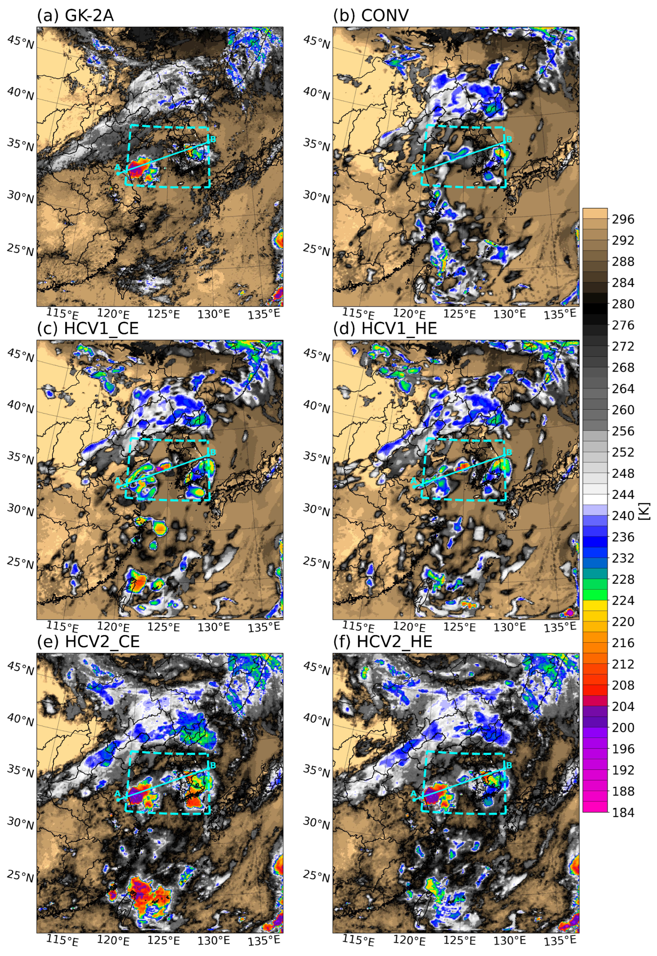
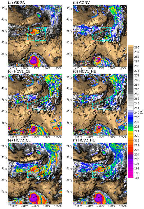
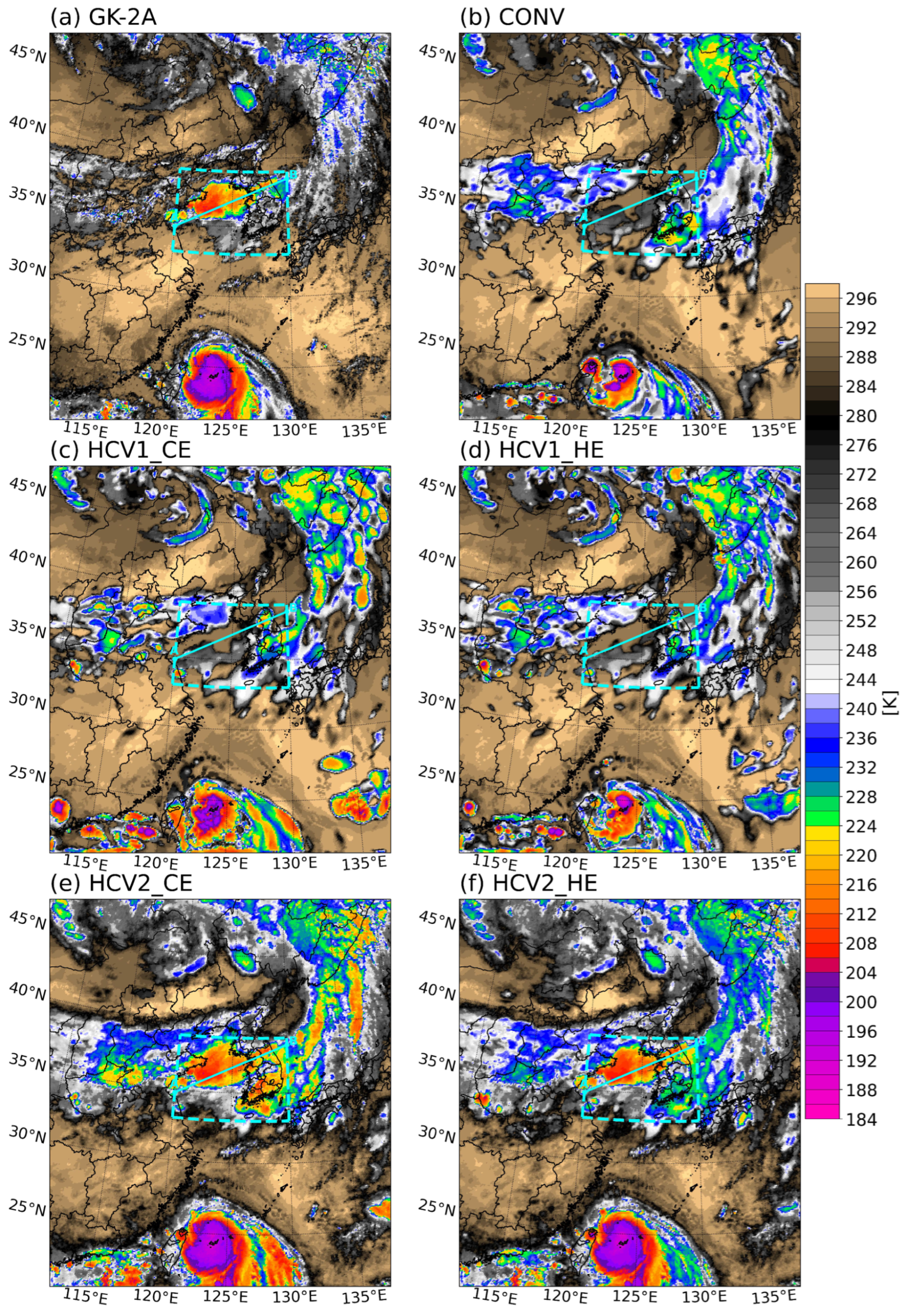
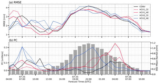
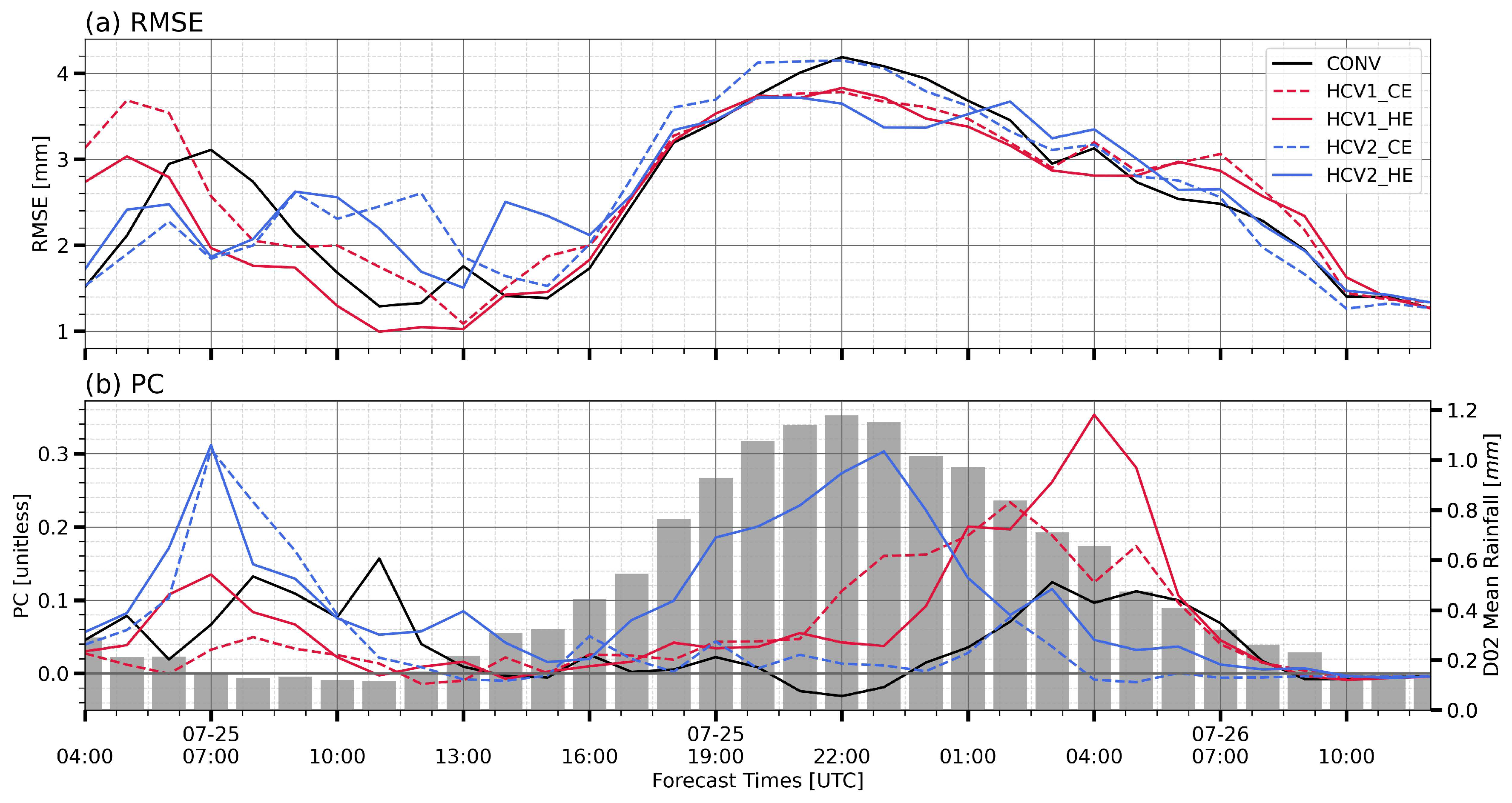
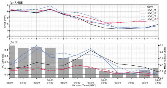
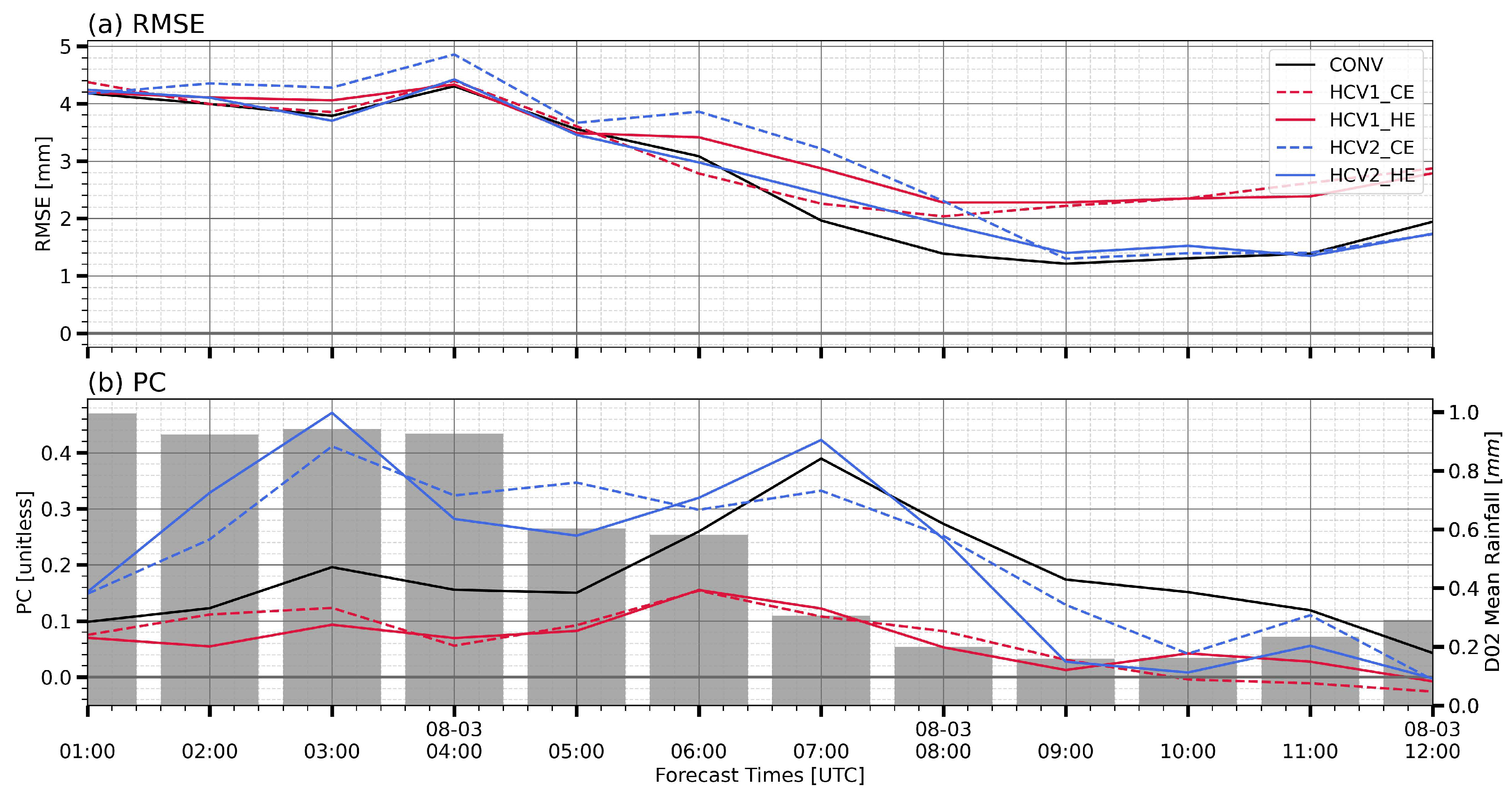

Disclaimer/Publisher’s Note: The statements, opinions and data contained in all publications are solely those of the individual author(s) and contributor(s) and not of MDPI and/or the editor(s). MDPI and/or the editor(s) disclaim responsibility for any injury to people or property resulting from any ideas, methods, instructions or products referred to in the content. |
© 2026 by the authors. Licensee MDPI, Basel, Switzerland. This article is an open access article distributed under the terms and conditions of the Creative Commons Attribution (CC BY) license.