


Highlights
What are the main findings?
- A village-scale winter wheat yield prediction framework was developed for coastal saline–alkali farmland by integrating Sentinel-2 data, topographic factors, and climatic variables.
- PGFI-XGBoost achieved stable predictive performance, while the Three-Stage Fusion XGBoost Model slightly improved final accuracy and provided process-based interpretation of the stress–growth–yield pathway.
What are the implications of the main findings?
- The framework can support village-level winter wheat yield prediction in coastal saline–alkali areas under strong spatial heterogeneity and multiple environmental stresses.
- SHAP-based interpretation helps identify key yield-limiting factors, such as geographic constraints, topography, and vegetation growth status, providing support for precision agricultural management.
Abstract
Accurately estimating village-level winter wheat yield in coastal saline–alkali farmland is challenging because this region has strong spatial differences and multiple environmental stresses. In this study, Huanghua City, Hebei Province, was selected as a typical coastal saline–alkali area. Sentinel-2 images, climate factors, and topographic variables, including elevation, topographic wetness index, distance to the coastline, and distance to water systems, were combined to build a phenology-guided feature set for winter wheat yield prediction in coastal areas. The results showed that Phenology-Guided Feature Integration XGBoost achieved an R2 of 0.6382 and an RMSE of 450.15 kg/ha, which was slightly better than Gradient Boosting (R2 = 0.6256) and Random Forest (R2 = 0.6098), and clearly better than SVR (R2 = 0.4792), Ridge regression (R2 = 0.4582), and a single Decision Tree (R2 = 0.3088). Then, a three-stage branch was designed to identify the main drivers of SI, NDVI, and winter wheat yield at different stages, helping explain how environmental constraints and vegetation responses jointly affect final yield. The Three-Stage Fusion XGBoost Model achieved an R2 of 0.6439, an RMSE of 446.24 kg/ha, and an MAE of 363.38 kg/ha, showing a slight improvement in prediction accuracy. SHAP analysis showed that SI, distance-related factors, elevation, TWI, and NDVI were important drivers of winter wheat yield variation. Spatial prediction results showed higher winter wheat yield in inland areas (5145 kg/ha) and lower yield in coastal areas (4198 kg/ha). This framework supports village-scale winter wheat yield prediction in coastal saline–alkali farmland and improves model interpretability.
1. Introduction
Food security is the cornerstone of national social stability and sustainable economic development, acting as a critical defense line against the challenges of global climate change [1]. For China, the world’s largest wheat producer, the stability of wheat production is directly related to national food reserve security and public well-being [2]. Against the backdrop of increasingly scarce arable land resources [3], the vast saline–alkali land resources in the Bohai Rim region are regarded as vital reserve arable land to guarantee national food security [3]. However, as a typical coastal plain saline area, the agro-ecosystem of Huanghua City in Hebei Province is extremely fragile, and crop growth has long been constrained by the shallow groundwater table and the intrusion effect of highly mineralized seawater [4]. This unique water–salt transport environment leads to a high degree of spatial heterogeneity and temporal dynamics in soil salinization [5], severely limiting the yield potential of winter wheat. Therefore, establishing a yield monitoring and prediction system capable of accurately deciphering crop growth mechanisms under such complex water–soil environments is crucial for guiding regional stress-resistant cultivation and formulating scientific agricultural development plans.
Traditional crop yield prediction methods mostly rely on field sampling surveys or empirical regression models based on meteorological data [6]. These methods are often constrained by poor timeliness, high labor costs, and their reliance on limited sample areas [7]. In contrast, satellite remote sensing technology, with its advantages of large-scale coverage and high spatiotemporal resolution [8], has become the mainstream method for crop yield estimation at the regional scale [9]. However, in regions experiencing severe water–salt stress, such as Huanghua City, relying solely on vegetation indices (VIs) often fails to fully capture the specific environmental pressures crops face during their growth processes [10]. This is because complex background factors, such as surface salinity and wet soil, often interfere with spectral signals, masking the true physiological stress status of the crop root zone [11] and leading to limited yield estimation accuracy for single remote sensing models in saline–alkali lands.
In recent years, to overcome the limitations of single data sources, domestic and international scholars have extensively explored multi-source data fusion and the application of machine learning algorithms, confirming the tremendous potential of multi-factor synergistic retrieval in crop yield estimation [12]. Han et al. (2020) [13] achieved broad-scale prediction of winter wheat yield in China based on multi-source data and machine learning algorithms, validating the effectiveness of integrating climate, soil, and remote sensing data for macroscopic yield estimation. At the regional scale, Li et al. (2025) [14] used Henan Province as the study area to screen key influencing factors via the XGBoost model, significantly enhancing the robustness and generalization ability of the winter wheat yield estimation model. Similarly, Shariati and Abbasi (2025) [15] further verified the applicability of this approach in winter wheat yield prediction by constructing machine learning models that integrate multi-source data. Furthermore, to dig deeper into the driving mechanisms of meteorological data on crop growth, Peng et al. (2024) [16] developed a spatio-temporal deep learning network combining weather forecasts and remote sensing data, effectively resolving the nonlinear mapping between meteorological factors and crop yield. In the specific domain of saline stress monitoring, Lu et al. (2025) [17] integrated Sentinel-2 multispectral information and soil salt content using the Random Forest (RF) algorithm, successfully improving the accuracy of winter wheat yield estimation under saline stress. However, despite significant progress in their respective fields, most of these studies adopt a predictive paradigm of “environment directly infers yield,” which overlooks the spatio-temporal heterogeneity of environmental factors. Specifically, geographical elements (e.g., topography, distance to features) are relatively static in the short term, while water–salt and meteorological factors fluctuate dynamically. This oversight leads to inadequate characterization of the cumulative and lagging effects of environmental stress on crop growth, limiting the model’s interpretability and cross-regional generalization. To address this deficiency, this study introduces a more refined “static constraint—dynamic driver” spatiotemporal environmental factor system. Specifically, we define the Digital Elevation Model (DEM), Topographic Wetness Index (TWI), and distances to water systems and coastlines extracted via OpenStreetMap (OSM) as static geographical constraint variables, maintaining them constant over the three-year study period to reflect relatively stable environmental backgrounds. Simultaneously, time-series soil Salinity Index (NDSI/SI), seawater level, temperature, and precipitation are defined as dynamic environmental stress variables. These are aggregated and calculated based on key phenological stages of winter wheat, such as sowing, green-up, and grain-filling stages, to capture the cumulative and lagging effects of water–salt and meteorological factors across different growth phases.
In terms of modeling strategy, traditional linear statistical models struggle to interpret the complex nonlinear interactions among the aforementioned multi-source heterogeneous data [18]. The XGBoost model, with its robustness and generalization capabilities when handling high-dimensional data, provides an efficient solution to this problem [19]. More importantly, village-level winter wheat yield prediction in coastal saline–alkali farmland is more relevant for practical agricultural management than county-level estimation. In saline–alkali regions, soil salinity, irrigation and drainage conditions, crop growth status, and field management practices often vary greatly within the same county. Therefore, county-level average yield may mask local low-yield areas and cannot fully support targeted soil improvement, irrigation planning, and village-based production decisions. To better characterize crop growth processes and reduce the limitations of the conventional “environment directly infers yield” black-box paradigm [20], this study developed two complementary XGBoost-based strategies for village-level winter wheat yield prediction in coastal saline–alkali farmland. The first is PGFI-XGBoost, a single-stage model for direct yield prediction using phenology-guided multi-source features. The second is the Three-Stage Fusion XGBoost Model, which integrates a single-stage main branch, a three-stage auxiliary branch, and an outer-cross-validation-based fusion strategy. In addition, SHAP was employed to quantify the contributions of key environmental, geographical, and vegetation-related factors.
- (1)
- To construct a phenology-based “static–dynamic” coupled feature set for village-level winter wheat yield prediction in coastal saline–alkali farmland and evaluate its effectiveness in capturing environmental stress and crop growth dynamics;
- (2)
- To develop a Three-Stage Fusion XGBoost Model for village-level winter wheat yield prediction by integrating direct yield prediction with stage-specific information on SI, NDVI, and yield formation;
- (3)
- To use the SHAP interpretability framework to identify the key drivers of village-level winter wheat yield variation in coastal saline–alkali farmland, including salinity-related indicators, distance to the coastline, distance to water systems, topographic factors, and vegetation indices.
2. Materials and Methods
2.1. Study Area
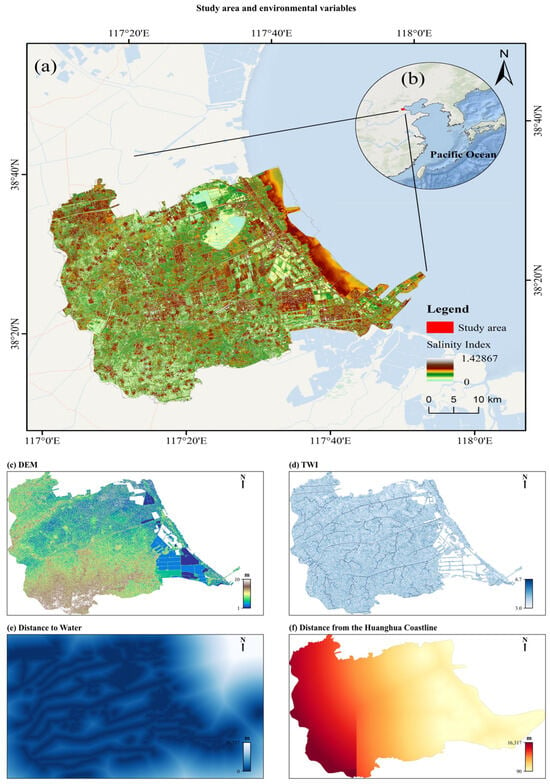
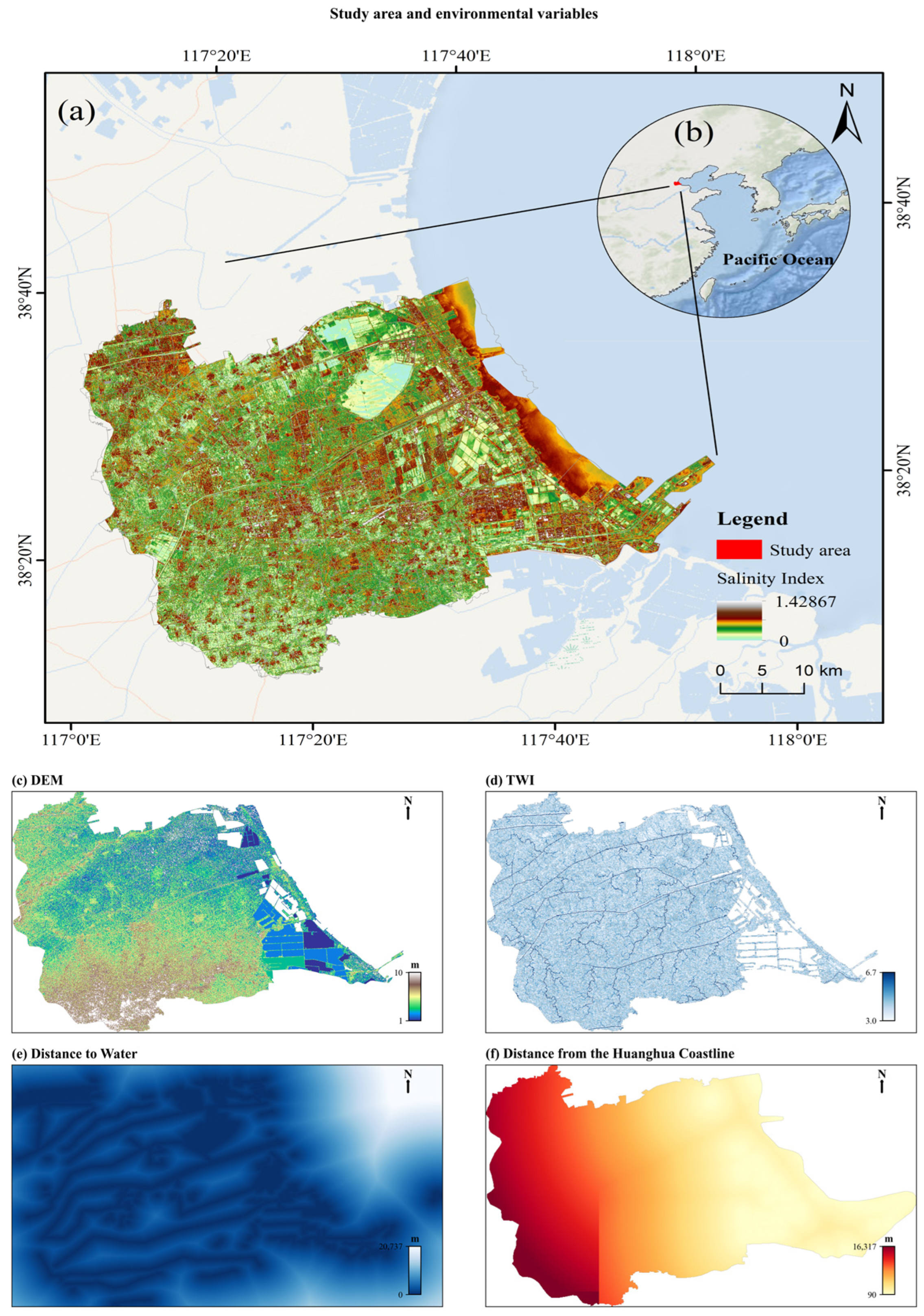
This study selects Huanghua City, Hebei Province, as a typical experimental area (Figure 1). Located in the eastern Hebei Plain and on the west coast of Bohai Bay, Huanghua City belongs to the South Canal water system of the Haihe River Basin. The average annual evaporation in Huanghua City is 1234.8 mm, which far exceeds its average annual precipitation of 544.9 mm. The soil types in this region are primarily coastal saline soil and fluvo-aquic soil, with the chemical composition of soil salinity mainly consisting of chlorides and carbonates.
Figure 1.
Geographical location and topographic features of Huanghua City. (a) Location in Hebei Province; (b) Location on the coast of the Bohai Sea (western Pacific); (c) elevation (DEM); (d) Topographic Wetness Index (TWI); (e) distance to primary water systems; (f) distance to coastline. Under intense evaporation, the soluble salts readily crystallize and precipitate on the soil surface, forming a white salt crust with high reflectivity. Since visible light bands (such as the red and blue bands) are highly sensitive to changes in the brightness and reflectivity of such salt crusts dominated by chlorides and carbonates, this study specifically selected the Salinity Index (SI) as the core remote sensing indicator [21]. The SI values in the study area range from 0.001 to 1.429 (Figure 1a,b). The band combination of the SI aligns closely with the spectral response characteristics of the main salt components in the Huanghua area, enabling highly sensitive detection of crust phenomena and thus accurately quantifying the intensity of abiotic stress (salinization) on the land surface (Figure 1a,b). The terrain is low-lying and flat, with elevations ranging from 1 to 31 m (Figure 1c), and the Topographic Wetness Index (TWI) distributed between 3.0 and 6.7 (Figure 1d). Influenced by its unique geographical location, the groundwater table in this region is extremely shallow, with a perennial burial depth mostly between 1.0 and 3.0 m, and its mineralization degree is exceptionally high, generally exceeding 5 g/L [4]. Significant gradient differences are observed in the distance to primary water systems (0–20,737 m, Figure 1e) and the distance to the coastline (90–16,317 m, Figure 1f). Long-term interactions of seawater intrusion and the monsoon climate result in significant seasonal accumulation characteristics of soil salinity within the tillage layer (0–40 cm) [14].
As a typical coastal saline agriculture area, agricultural production in Huanghua City is dominated by a winter wheat-summer maize crop rotation system. Under this cropping system, the autumn sowing and spring green-up stages of winter wheat coincide perfectly with the regional “peak salt return period,” characterized by scarce precipitation and intense surface evaporation. Consequently, the widely distributed saline–alkali patches in this region significantly inhibit the emergence rate of winter wheat and are prone to inducing “physiological drought” stress caused by high osmotic pressure environments, further constraining wheat population growth and yield [12]. This water–salt environment, featuring both significant spatial heterogeneity and strong temporal dynamic changes, makes Huanghua City an ideal experimental area for studying crop growth response mechanisms and refined yield estimation methods under complex saline stress conditions [11].
2.2. Data Collection and Processing
2.2.1. Multi-Source Remote Sensing Data
To comprehensively capture the nonlinear coupling features of the “soil-climate-vegetation” system during the growth of winter wheat in coastal saline areas, this study constructed high-dimensional spatio-temporal datasets encompassing multi-source remote sensing imagery, meteorological driving data, and static geographical environment features. This data system comprises a total of 113 feature variables (TIF raster files, see Supplementary Materials), spanning the complete growth cycles of winter wheat from 2020 to 2023. Significant differences exist among these data types regarding spatial resolution, temporal scale, and physical meaning. To ensure interpretability and consistency in subsequent modeling and analysis, this section systematically describes the data sources, index construction, and preprocessing workflows.
Based on Sentinel-2 multi-spectral remote sensing imagery, and combined with the growth characteristics of winter wheat in coastal saline lands within the study area, this paper selected five spectral indices sensitive to saline stress responses (Table 1). These indices characterize crop physiological states from the perspectives of vegetation nitrogen status, canopy moisture conditions, and surface salinity information. To mitigate the instability of single-date remote sensing observations and to highlight the temporal differences in saline stress effects across different growth stages, the spectral indices were integrated and reconstructed in stages according to winter wheat phenology [13].
Table 1.
Multi-source Remote Sensing Spectral Indices.
Ultimately, across three growing seasons from 2020 to 2023, a total of 90 time-series feature layers at the phenological stage scale (5 spectral indices × 6 growth stages × 3 years) were generated. These serve as the primary remote sensing input variables for subsequent staged modeling and yield estimation. The calculation methods for each spectral index and their functional descriptions for monitoring saline stress are detailed in Table 1.
2.2.2. Static Geographical Environment Features
Considering the significant spatial heterogeneity of water–salt transport processes in coastal saline areas, relying solely on dynamic variables like remote sensing and meteorology is insufficient to fully characterize the underlying constraint conditions of the land. This study further introduces multiple static geographical environment features (Table 2) as crucial covariates describing topographic patterns, salt accumulation potential, and anthropogenic disturbance intensity. These assist in explaining the stable spatial variation characteristics of winter wheat yield.
Table 2.
Description of static geographical environment features.
2.2.3. Meteorological Driving Data
Meteorological conditions heavily influence winter wheat growth in coastal saline areas by regulating crop evapotranspiration intensity, soil moisture dynamics, and salt migration processes [13]. This study acquired daily average temperature (Tem) and precipitation (Pre) raster data for the study area over the same period (Table 3), utilizing them as key driving factors to describe climate stress and water–salt dynamic changes [11].
Table 3.
Spatial resolution and indicator significance of meteorological driving variables.
Under typical rain-fed agricultural conditions in Huanghua City, precipitation events directly determine the leaching intensity and redistribution patterns of soil salinity. Particularly during the green-up and grain-filling stages, temporal fluctuations in precipitation play a decisive role in alleviating salt stress and ensuring grain filling. Concurrently, temperature indirectly regulates the soil water–salt balance by affecting crop physiological metabolic rates and evapotranspiration demands. Therefore, incorporating average temperature (Tem) and precipitation (Pre) into the model helps delineate the dynamic response features of crop growth processes regulated by climatic factors under saline stress (Table 3).
2.2.4. Data Cleaning and Spatiotemporal Alignment
Due to differences in spatial resolution, coordinate systems, and temporal scales among multi-source datasets, data cleaning, dynamic spatial alignment, and phenology-based temporal aggregation were conducted before constructing the village-level feature table.
- (1)
- Remote Sensing Data Cleaning: To reduce cloud and cirrus interference in Sentinel-2 imagery, a cloud mask was generated using the QA60 band. Opaque cloud and cirrus pixels were removed, and invalid values were set to NaN.
- (2)
- To ensure the consistent integration of multi-source remote sensing, meteorological, topographic, and spatial distance variables at the village scale, this study used village-level spatial aggregation to integrate multi-source variables at the village scale [8]. Village boundaries were aligned with each raster dataset, and the mean values of valid pixels within each village were extracted to generate unified village-level features for yield modeling.
Specifically, Sentinel-2-derived vegetation and salinity-related indices, including NDVI, NDRE, LSWI, and SI, were extracted at 10 m resolution. DEM and TWI were used at 30 m and 90 m resolutions, respectively. Distance variables, including distance to water bodies and distance to the Huanghua coastline, were derived from vector data through Euclidean distance transformation and generated at 30 m resolution. Meteorological variables, including Tem and Pre, were retained at their original 0.1° × 0.1° resolution.
In the temporal dimension, all variables were aligned according to the six key phenological stages of winter wheat, including overwintering, greening, jointing, heading, filling, and maturity. Sentinel-2 images were composited within the corresponding phenological windows, and meteorological variables were aggregated over the same periods. Through this spatiotemporal alignment procedure, multi-resolution and multi-temporal data were converted into village-year samples suitable for machine learning modeling.
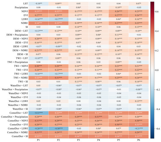
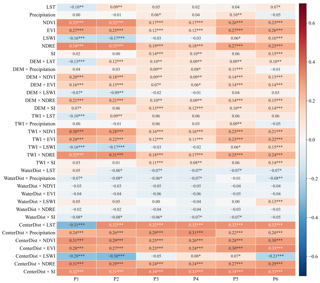
Figure 2 shows the correlation analysis between input features and winter wheat yield, providing a basis for subsequent feature selection and model interpretation.
Figure 2.
Heatmap of correlation between winter wheat yield and input features. P1–P6 represent overwintering, reviving/green-up, jointing, heading, grain-filling, and maturity stages, respectively. Values in cells indicate Pearson correlation coefficients. Asterisks indicate statistical significance: * p < 0.05, ** p < 0.01, and *** p < 0.001.
2.2.5. Collection of Yield and Village Boundary Data
Yield data were derived from official statistical records and retrieved from the AREMOS Chinese Agricultural Statistical Database, which integrates official agricultural statistical data. In the official wheat-yield survey system, wheat production is generally determined from sown-area surveys and unit-yield measurements, where sown area is estimated from sampled villages and area plots, and unit yield is obtained through crop-cutting measurements using 3–5 small quadrats of 10 square chi in sampled fields before harvest. Total wheat production is then calculated as sown area multiplied by average unit yield. To ensure reproducibility, the detailed data acquisition methods and derivation scripts are available at https://github.com/c2581252165-hue/PGFI-XGBoost-data-acquisition (accessed on 24 May 2026).
Village boundary data were provided by the Geographic Remote Sensing Ecological Network Platform (http://www.gisrs.cn).
2.3. Feature Engineering
2.3.1. Winter Wheat Phenology Division
Crop sensitivity to saline stress varies significantly across different growth stages. Based on long-term phenological observation data in Huanghua City, the complete growth cycle of winter wheat was divided into six key physiological stages: Overwintering (P1), Green-up (P2), Jointing (P3), Heading (P4), Grain-filling (P5), and Maturity (P6) (Table 4).
Table 4.
Division of Winter Wheat Phenological Stages.
2.3.2. Phenology-Based Median Compositing Method
Addressing the pervasive issues of cloud cover, aerosol interference, and shadow noise in optical remote sensing imagery in coastal areas, traditional single-date imagery struggles to stably reflect true crop growth conditions. Consequently, this study employed a phenology-based median compositing method to reconstruct time-series remote sensing features.
Assuming that a certain phenological stage M3 contains n available images, for any given pixel (x, y), its feature value VT(x, y) is calculated as follows:
where Vi(x,y) represents the observation value of image i. Median filtering not only effectively removes noise from clouds (bright extremes) and shadows (dark extremes) but also generates robust features representing the average growth status of that phenological stage, significantly enhancing the usability and physical interpretability of time-series data.
2.4. Research Methods
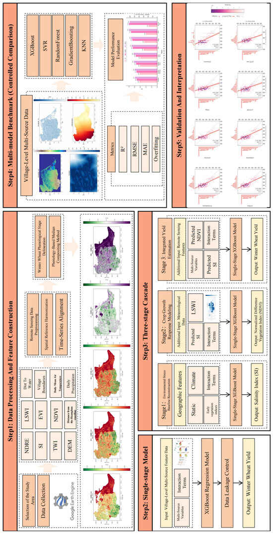
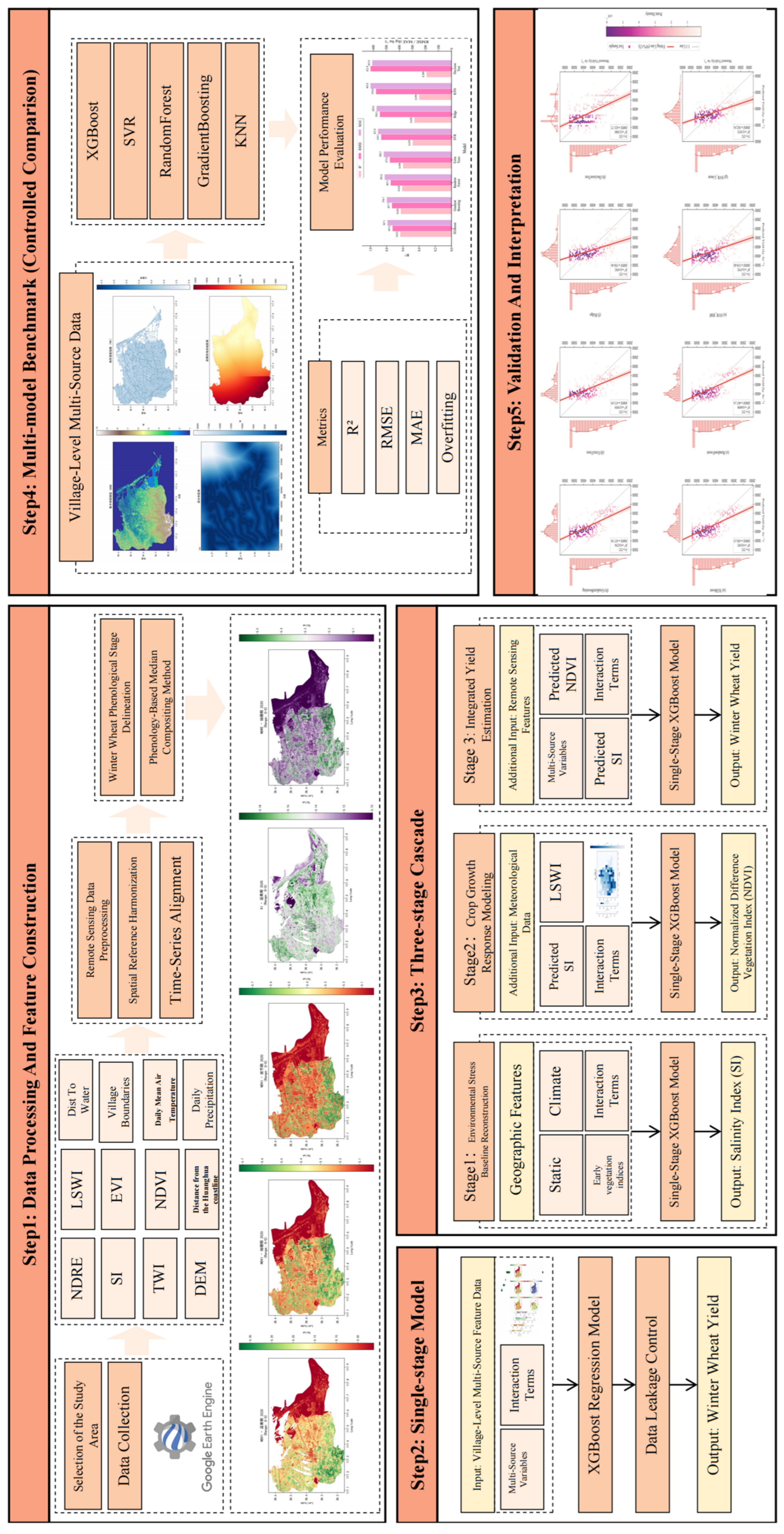
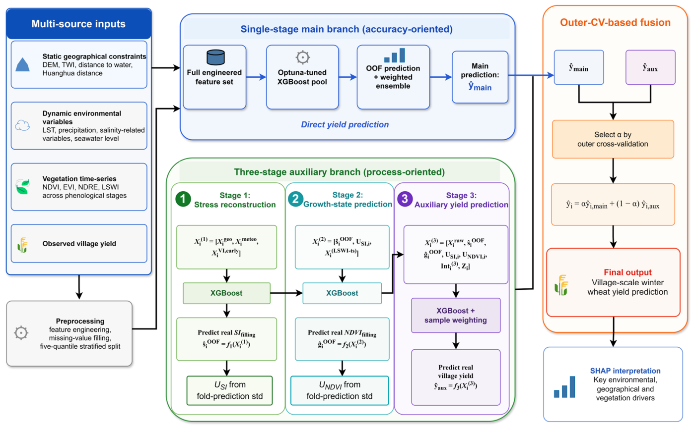
This study proposes an XGBoost-based framework for village-level winter wheat yield prediction in coastal saline–alkali farmland and integrates phenology-guided feature construction, a three-stage auxiliary branch, and a fusion strategy, as shown in Figure 3. The code was written and managed using Visual Studio Code 1.101.2 (Microsoft Corporation, Redmond, WA, USA; https://code.visualstudio.com/).
Figure 3.
The framework of the proposed methods.
2.4.1. PGFI-XGBoost (Phenology-Guided Feature Integration XGBoost)
To characterize the impact of multi-source environmental factors on winter wheat yield at different growth stages, this study selected the eXtreme Gradient Boosting regression model as the core algorithm. By iteratively constructing an additive decision tree ensemble structure, the model utilizes second-order gradient information of the loss function to optimize the model during each training round, thereby effectively depicting complex nonlinear relationships among features. The detailed parameter configuration of PGFI-XGBoost is provided in Appendix A, Table A1.
Its objective function consists of two parts: a training loss term and a regularization term.
where l is a differentiable convex loss function that measures the difference between the predicted value yi and the true value yi; Ω(fk) is the regularization term, which controls the complexity of the tree and is defined as:
In the formula, T represents the number of leaf nodes, w denotes the leaf node weights, and γ and λ are penalty coefficients that control model overfitting.
2.4.2. Three-Stage Fusion XGBoost Model
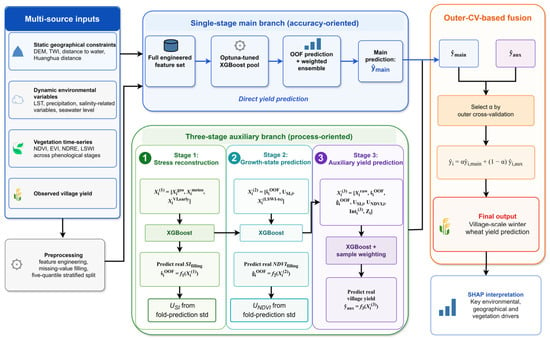
To complement the direct predictive capability of the single-stage model, this study developed a Three-Stage Feature-Augmented Fusion XGBoost model (Figure 4). The model consists of a single-stage main branch, a three-stage auxiliary branch, and an out-of-fold cross-validation-based fusion strategy.
Figure 4.
Framework of the Three-Stage Fusion XGBoost Model.
In the three-stage auxiliary branch, the soil salinity level (SI), which represents salinity stress, was first predicted using temperature, precipitation, terrain-related variables, spatial distance variables, and other environmental factors. Second, based on the predicted SI together with water- and vegetation-related features, NDVI was further predicted to represent crop growth status under the corresponding salinity condition. Third, the predicted SI and NDVI were used as intermediate process-related variables and incorporated into the subsequent yield prediction model together with the original multi-source features, such as EVI, climatic variables, terrain factors, and distance-related variables. Therefore, it should be noted that the proposed model does not simply formulate the prediction process as a linear “SI–NDVI–yield” pathway. Instead, it comprehensively considers the combined effects of salinity stress, crop growth, climate, terrain, and spatial environmental factors on village-level wheat yield prediction. The final yield prediction can be expressed as:
where ŷi, main and ŷi, aux denote the predictions of the single-stage main branch and the three-stage auxiliary branch, respectively. The fusion coefficient α was determined using outer five-fold cross-validation within the training set. The median fusion coefficient α was 0.56, assigning 56% weight to the main branch and 44% to the auxiliary branch.
ŷi = αŷi,main + (1 − α) ŷi,aux
To avoid information leakage, all intermediate predictions passed between stages were generated in an out-of-fold (OOF) manner. The training set was divided into five folds. For each fold, the intermediate prediction was generated by a model trained on the remaining four folds. For the independent test set, predictions from the five-fold-specific models were averaged.
In Stage 1, the model predicted the filling-stage salinity index using static geographical features, meteorological features, and early-stage vegetation features:
where Xigeo represents static geographical features, Ximeteo represents meteorological features, and Xi(VI,early) represents early-stage vegetation index features. The supervised target of Stage 1 is the true filling-stage salinity index of sample i, and the prediction is formulated as:
where ŝiOOF denotes the out-of-fold prediction of filling-stage SI. The uncertainty of Stage 1 was quantified as the standard deviation of predictions from the five fold-specific XGBoost models:
where ŝi,k denotes the prediction from the K-th fold-specific model, and is the mean prediction across the five models.
Xi(1) = [Xigeo, Ximeteo, Xi(VI,early)]
ŝiOOF = f1(Xi(1)), si = SIfilling,I
In Stage 2, the input feature vector is denoted as Xi(2), and its composition is defined as:
where ŝiOOF is the out-of-fold prediction generated by Stage 1, USI,i is the uncertainty of Stage 1, and Xi(LSWI-ts) denotes the LSWI time-series features. The supervised target of Stage 2 is the true filling-stage NDVI of sample i, and the prediction is formulated as:
Xi(2) = [ŝiOOF, USI,i, Xi(LSWI-ts)]
ĝiOOF = f2(Xi(2), ŝiOOF, USI,i), gi = NDVIfilling,i
Similarly, the uncertainty of Stage 2 was calculated as the standard deviation of the five fold-specific NDVI predictions:
where ĝi,k denotes the prediction from the k-th fold-specific model, and is the mean prediction across the five models.
In Stage 3, the input feature vector is denoted as Xi(3), and its composition is defined as:
where Xiraw represents the original numerical features, ŝiOOF and ĝiOOF denote the out-of-fold predictions from the previous two stages, USI,i and UNDVI,i denote the uncertainties of the previous two stages, Inti(3) represents the Stage 3 interaction features, and Zi denotes township-level statistical encoding features. The supervised target of Stage 3 is the true village-level winter wheat yield of sample i, and the prediction is formulated as:
Xi(3) = [Xiraw, ŝiOOF, ĝiOOF, USI,i, UNDVI,i, Inti(3), Zi]
ŷi,aux = f3(Xi(3)), yi = Yi
Finally, the direct yield prediction and the three-stage process-based prediction were integrated using the fusion strategy in Equation (4). This design was used to combine the direct relationship between multi-source features and yield with process-related information from the intermediate SI and NDVI predictions, rather than relying only on a single yield prediction pathway.
2.4.3. Model Validation and Evaluation
The Coefficient of determination (R2), Root Mean Squared Error (RMSE), and Mean Absolute Error (MAE) were selected as accuracy evaluation metrics [14].
In these equations, n is the total number of samples, yi is the measured yield, is the model-predicted yield, and is the mean of the measured yields, an R2 value closer to 1 and lower RMSE and MAE values indicate stronger explanatory power and higher prediction accuracy of the model.
3. Results
3.1. Village-Level Winter Wheat Yield Estimation in Coastal Saline–Alkali Farmland Using PGFI-XGBoost
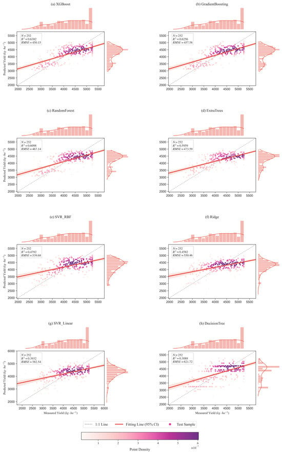
The PGFI-XGBoost model achieved an R2 of 0.6382 and an RMSE of 450.15 kg/ha on the test set. To further evaluate its predictive performance, this study compared it with several commonly used machine learning models, including Gradient Boosting, Random Forest, Extra Trees, SVR, Ridge, KNN, and Decision Tree. The results showed that PGFI-XGBoost slightly outperformed the ensemble tree-based models Gradient Boosting (R2 = 0.6256) and Random Forest (R2 = 0.6098), and clearly outperformed SVR (R2 = 0.4792), Ridge regression (R2 = 0.4582), and a single Decision Tree (R2 = 0.3088) (Figure 5). This indicates that PGFI-XGBoost has a stronger ability to capture the complex nonlinear relationships between environmental variables and winter wheat yield in coastal saline farmland [24].
Figure 5.
Scatter plots of measured versus predicted winter wheat yield for different machine learning models.
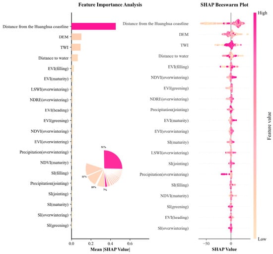
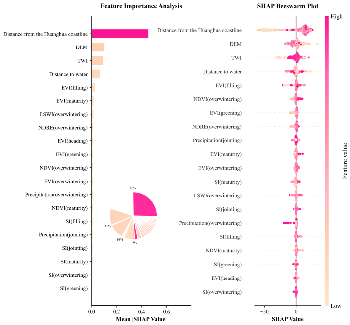
Feature importance analysis based on SHAP values further revealed the main driving factors of yield estimation (Figure 6). Geospatial variables played a dominant role in the model. Among them, the distance from the Huanghua coastline was the most important feature, with an average SHAP value of 0.45, much higher than that of other variables. This result may be closely related to the spatial distribution pattern of soil salinization in the study area, where areas closer to the coast are generally subject to stronger salinity stress. Elevation (DEM, 0.10) and the topographic wetness index (TWI, 0.09) also showed high importance, indicating that micro-topographic variation has an important influence on water–salt redistribution. In terms of vegetation indicators, EVI during the grain-filling and maturity stages contributed substantially to yield prediction, suggesting that crop growth status in the middle and late growth stages is closely associated with final yield [25]. In addition, overwintering vegetation indices, such as LSWI and NDRE, also showed high importance, indicating that early crop survival and growth conditions can provide useful information for yield estimation.
Figure 6.
Feature importance ranking of the PGFI-XGBoost model. Only feature-importance proportions greater than 3% are labeled in the inset pie chart for clarity.
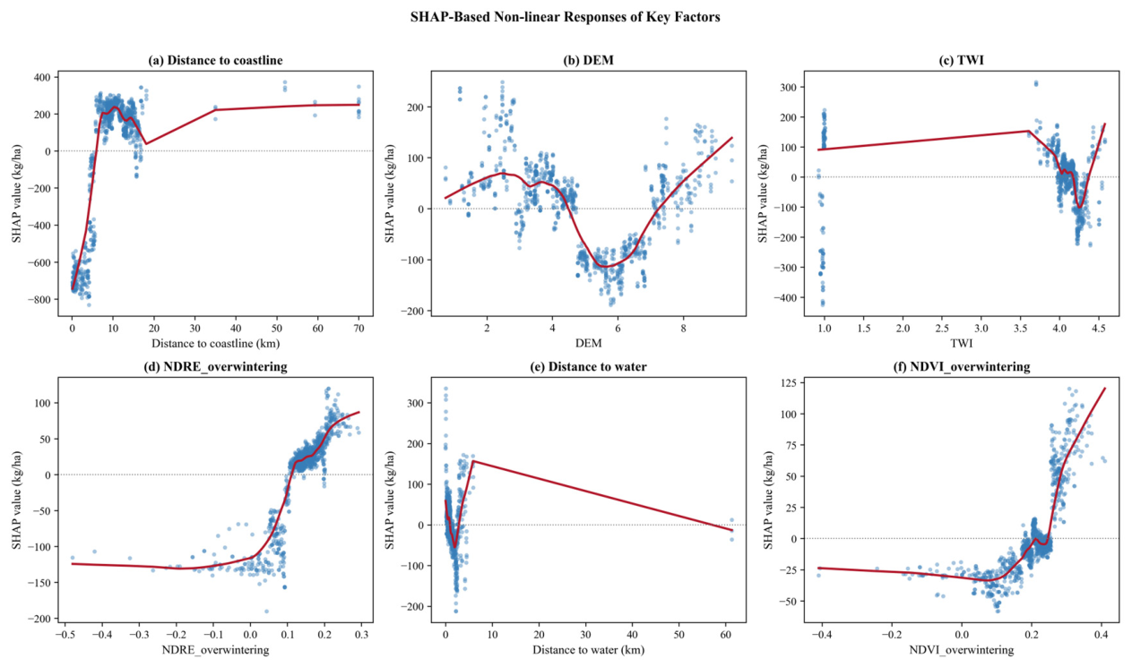
SHAP Dependence Plots further demonstrated that the relationships between key factors and yield are non-linear (Figure 7). The distance to coastline exhibited a clear threshold effect at approximately 7 km, beyond which the marginal contribution to yield diminished substantially.
Figure 7.
SHAP Dependence Plots for key factors in the PGFI-XGBoost model. Each subplot shows the relationship between a feature value (x-axis) and its SHAP contribution to yield prediction (y-axis), revealing non-linear threshold effects.
3.2. Three-Stage Fusion XGBoost Model for Village-Level Winter Wheat Yield Prediction in Coastal Saline–Alkali Farmland
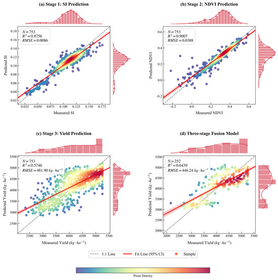
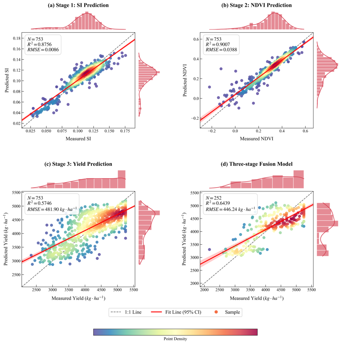
The results of the Three-Stage Fusion XGBoost Model showed that the intermediate variables could be predicted with relatively high accuracy. In Stage 1, the model achieved an R2 of 0.8756 and an RMSE of 0.0086 for SI prediction (Figure 8a). In Stage 2, the model achieved an R2 of 0.9007 and an RMSE of 0.0388 for NDVI prediction (Figure 8b). In Stage 3, the three-stage yield prediction model achieved an R2 of 0.5746 and an RMSE of 481.90 kg/ha (Figure 8c). After integrating the three-stage structure into the fusion framework, the final Three-Stage Fusion XGBoost Model achieved an R2 of 0.6439 and an RMSE of 446.24 kg/ha (Figure 8d), outperforming the standalone three-stage yield prediction branch. These results indicate that the fusion strategy can effectively combine direct yield prediction with process-related complementary information from the three-stage branch, thereby improving the accuracy and robustness of winter wheat yield estimation.
Figure 8.
Scatter plots of measured versus predicted values for the Three-Stage Fusion XGBoost Model: (a) SI prediction, (b) NDVI prediction, (c) three-stage yield prediction, and (d) three-stage fusion yield prediction.
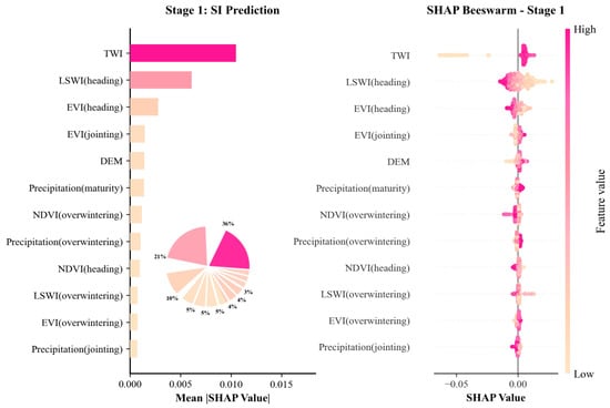
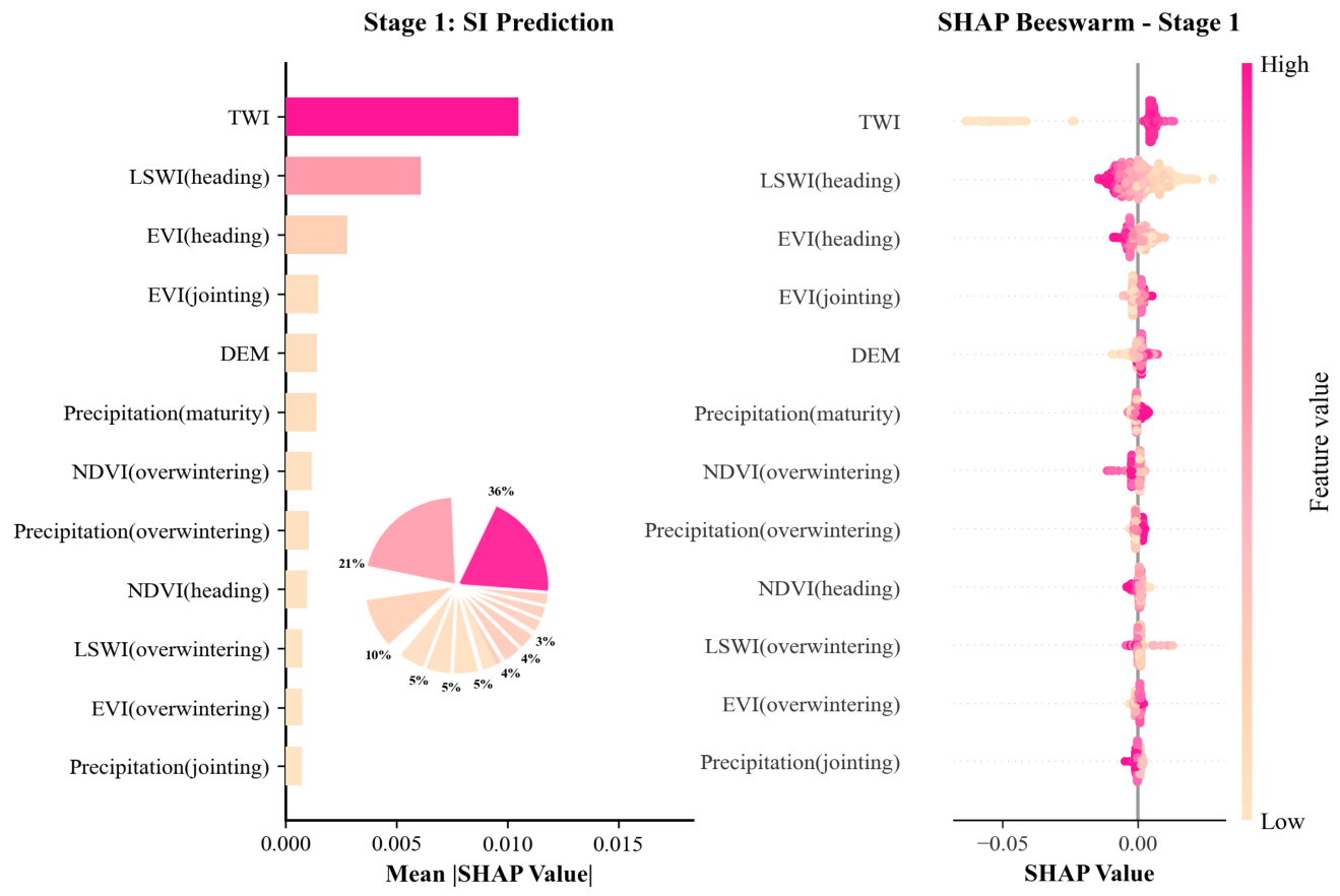
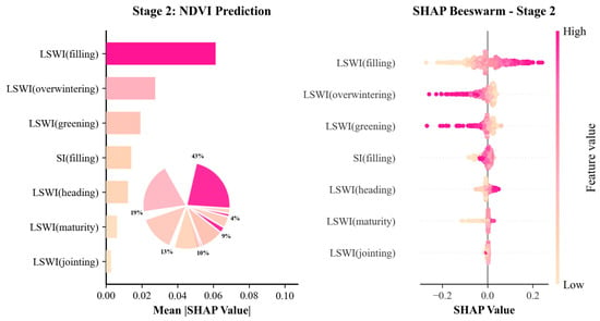
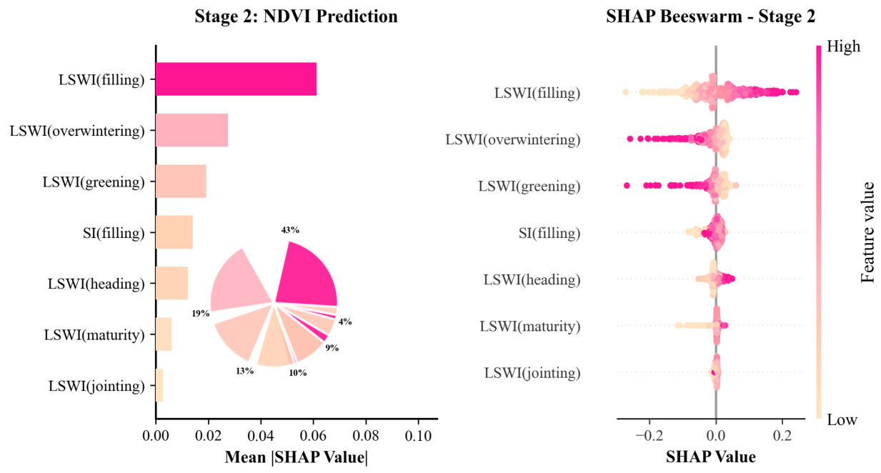
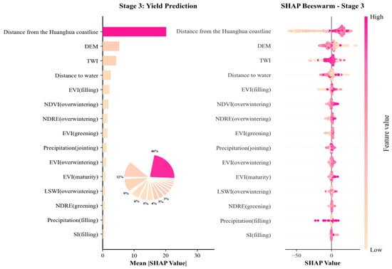
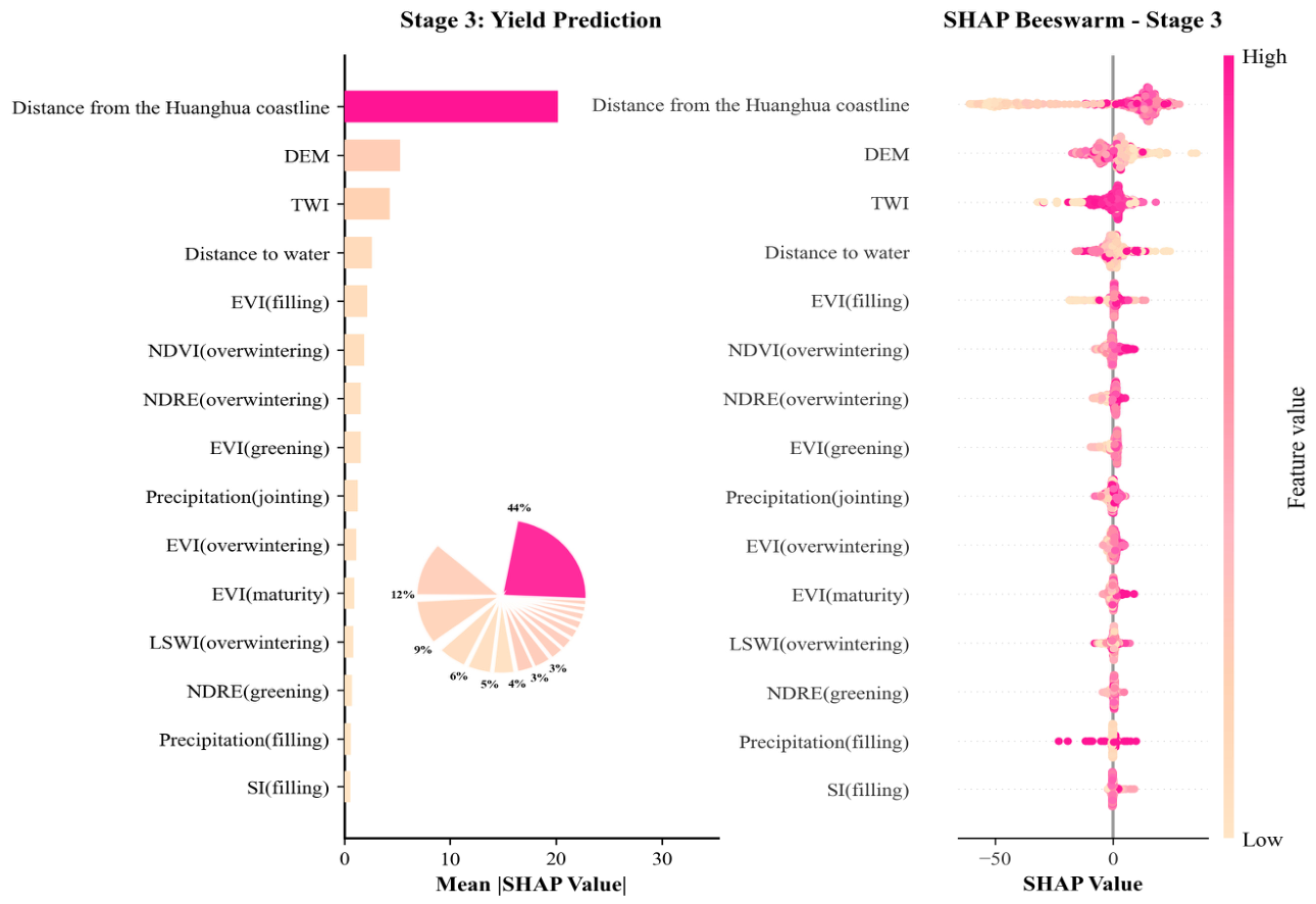
Feature importance analysis (Figure 9, Figure 10 and Figure 11) further supports this process-based interpretation. In Stage 1, TWI was the most important factor, indicating that topographic conditions strongly influenced the spatial distribution of soil water and salt [26]. In Stage 2, LSWI time-series features, especially those during the grain-filling, overwintering, and green-up stages, played a dominant role, suggesting a close relationship between crop water status and vegetation growth. In the final yield prediction stage, geospatial variables such as distance from the Huanghua coastline, DEM, and TWI remained important limiting factors. Meanwhile, EVI during the grain-filling stage, NDVI during the overwintering stage, and the predicted SI also contributed substantially to yield estimation. These results demonstrate that the Three-Stage Fusion XGBoost Model can effectively combine geographic constraints, vegetation dynamics, and process-related intermediate variables, thereby improving both prediction performance and interpretability.
Figure 9.
Feature importance ranking of Stage 1 in the Three-Stage Fusion XGBoost Model. Only feature-importance proportions greater than 3% are labeled in the inset pie chart for clarity.
Figure 10.
Feature importance ranking of Stage 2 in the Three-Stage Fusion XGBoost Model. Only feature-importance proportions greater than 3% are labeled in the inset pie chart for clarity.
Figure 11.
Feature importance ranking of Stage 3 in the Three-Stage Fusion XGBoost Model. Only feature-importance proportions greater than 3% are labeled in the inset pie chart for clarity.
3.3. Residual Sensitivity Analysis Under Salinity-Related Heterogeneity
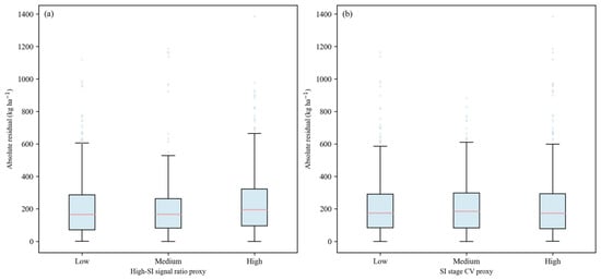
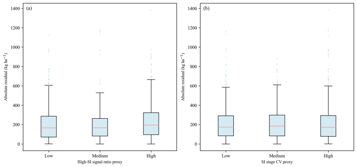
To examine whether salinity-related heterogeneity affected prediction stability, a residual sensitivity analysis was conducted using two proxy indicators: the high-SI signal ratio and the SI stage coefficient of variation. For the high-SI signal ratio proxy, the low, medium, and high groups corresponded to values of 0, 0.167, and 0.333–1.000, respectively, representing relatively normal cropland, transitional cropland with localized salinity patches, and saline-affected cropland mixed with persistent high-salinity or abandoned saline patches. For the SI stage coefficient of variation proxy, the low, medium, and high groups corresponded to 0.033–0.097, 0.097–0.148, and 0.148–0.729, respectively, representing stable, moderately variable, and highly variable SI dynamics across phenological stages.
As shown in Figure 12a, villages with a higher proportion of persistent high-SI signals showed larger absolute residuals, with mean absolute residuals of 212.51, 216.34, and 247.18 kg ha−1 for the low, medium, and high groups, respectively, and the difference was significant (p = 0.023). This indicates that villages containing more persistent high-salinity patches tended to have larger model errors. In contrast, Figure 12b shows that the SI stage coefficient of variation did not significantly affect model residuals (p = 0.963), suggesting that the prediction errors were not mainly caused by temporal fluctuations of SI across different phenological stages, but were more likely related to the spatial persistence of salinity patches within villages, mixed land use, and uncertainty in village-level yield statistics.
Figure 12.
Residual sensitivity analysis under different salinity-related heterogeneity proxy levels. (a) Absolute residual distribution grouped by the high-SI signal ratio proxy. (b) Absolute residual distribution grouped by the SI stage coefficient of variation proxy.
Overall, salinity-related heterogeneity may partly contribute to village-level prediction uncertainty, especially in villages with persistent high-SI signals.
However, field management differences, abandoned saline patches, transitional zones, and mixed land use may also jointly contribute to prediction errors.
3.4. Spatial Distribution Pattern of Village-Level Winter Wheat Yield in Coastal Saline–Alkali Farmland
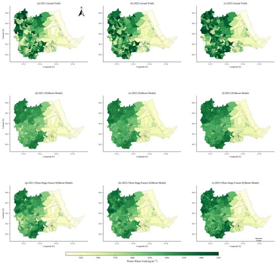
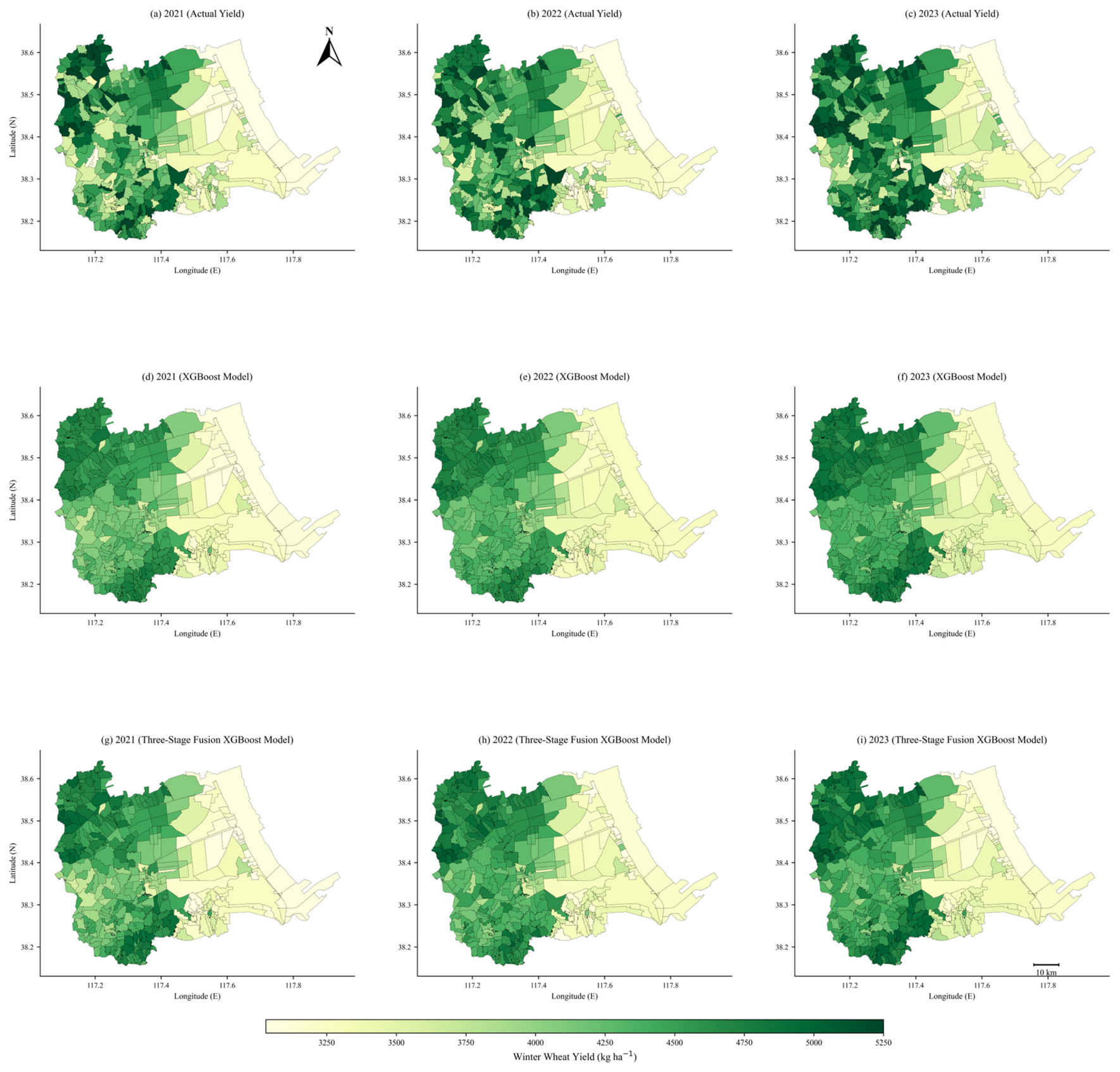
Figure 13 compares the spatial distribution of winter wheat yield in 2021–2023 using observed yield (Actual Yield), the XGBoost Model, and the Three-Stage Fusion XGBoost Model. The two model outputs show highly consistent spatial patterns with the observed map and both capture the clear spatial heterogeneity of yield across Huanghua City.
Figure 13.
Spatial distribution of winter wheat yield in Huanghua City from 2021 to 2023: comparison among Actual Yield, XGBoost Model, and Three-Stage Fusion XGBoost Model.
At the regional scale, the overall estimates of the two models are very close. For 2021, the mean predicted yield is 4135 kg/ha for the XGBoost Model and 4142 kg/ha for the Three-Stage Fusion XGBoost Model. For 2022, the corresponding means are 4210 and 4209 kg/ha. For 2023, they are 4302 and 4297 kg/ha, respectively. Across the three years, the average levels of the two models are nearly identical (approximately 4216 kg/ha), indicating comparable regional estimation capability.
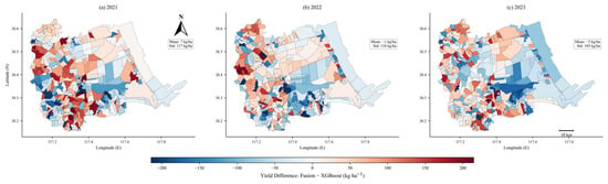
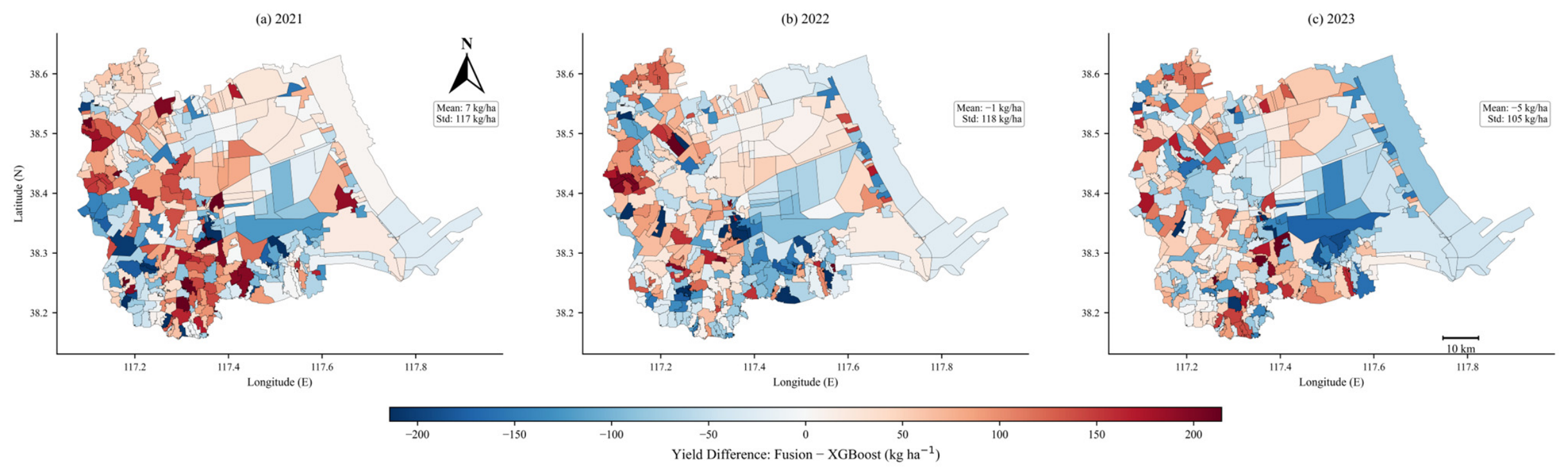
The difference map (Figure 14, Fusion—XGBoost) further reveals that inter-model differences are moderate but spatially structured. The mapped difference range is −247 to +247 kg/ha. The annual mean differences are +7 kg/ha (2021), −1 kg/ha (2022), and −5 kg/ha (2023), with annual standard deviations of 117, 118, and 105 kg/ha, respectively. These results indicate that the two models are broadly consistent while still showing local discrepancies in specific zones.
Figure 14.
Spatial difference between model predictions (Three-Stage Fusion XGBoost Model minus XGBoost Model) for 2021–2023.
Spatially, both models reproduce a stable gradient pattern: relatively high-yield areas are concentrated in inland central-southwestern regions, whereas lower-yield areas are mainly distributed in the eastern coastal zone, which is consistent with local water–salt constraints and salinity stress conditions [27,28,29]. In inland high-yield patches, the fusion model tends to produce slightly higher values in some locations, while in coastal low-yield patches it tends to produce slightly lower values in some locations.
Although the two models are similar in regional-scale predictive level, the Three-Stage Fusion XGBoost Model provides better process interpretability by explicitly organizing predictions into stress-related and growth-related intermediate links. This process-aware structure helps support agronomic interpretation and management-oriented decision-making.
4. Discussion
4.1. Scale Effects and the Value of Village-Level Yield Prediction
In this section, we primarily address the question: why may village-level yield prediction obtain lower R2 values than some county- or regional-scale studies, and why is village-level prediction still important for agricultural management? This study developed a winter wheat yield prediction system based on village-level samples (n = 1005). Under a unified data split (training/test = 753/252) and consistent feature engineering conditions, PGFI-XGBoost, the Three-Stage Fusion XGBoost Model, and several baseline models were systematically compared. To further examine the spatial mixing between training and test samples, the quadrant-based mixed-village proportions are provided in Appendix A, Table A2.
The possible reason for the relatively lower R2 at the village scale could be the stronger influence of local heterogeneity. Compared with county- or regional-scale yield estimation, village-level yield is more strongly affected by field management, crop varieties, fertilizer and irrigation inputs, soil patchiness, drainage conditions, and salinity stress [30]. These local factors make the relationship between remote sensing or meteorological variables and yield more unstable [11,30]. Previous county-level winter wheat studies have reported R2 values above 0.75 [13], which are higher than the village-level R2 obtained in this study [31,32]. This difference is reasonable because county-level yield values are spatially aggregated and can smooth part of the local noise, leading to more stable correlations and, in some cases, higher evaluation metrics. Therefore, the R2 obtained at the village scale may be lower than that reported in some macro-scale studies, which reflects the higher difficulty of fine-scale yield prediction in heterogeneous saline–alkali farmland.
However, village-level prediction has clearer practical value for agricultural management. County-level averages may mask local low-yield areas and cannot fully represent the internal differences among villages [30]. In contrast, village-level prediction can provide more detailed information for identifying low-yield zones, guiding targeted soil improvement, optimizing irrigation and drainage planning, and supporting village-based production decisions. Therefore, although village-level prediction is more difficult, it is more directly related to practical agricultural management in coastal saline–alkali areas.
4.2. Effectiveness of Feature Engineering and Phenological Stage Information
Based on the original 46 numerical features, this study constructed a series of time-series statistical features, including interaction terms, ratio terms, inter-stage changes, ranges, and means. After incorporating township-level statistical features, a 118-dimensional feature set was formed, which substantially enhanced the ability of tree-based models to represent nonlinear relationships and stage-coupled processes.
This design is consistent with the general understanding in remote sensing-based yield prediction: crop yield is not determined by a single temporal index, but is jointly influenced by cumulative stress and recovery processes across different phenological stages. Therefore, the use of stage-based temporal variation and integrated statistical indicators is necessary to describe the crop growth trajectory [32,33,34]. In multi-source fusion frameworks, weather and remote sensing variables are often encoded as time-series signals to improve prediction stability, suggesting that temporal structure itself is a key factor affecting yield prediction performance rather than an optional addition [31,34].
The interaction features constructed in this study, such as LST × Precipitation and NDVI × LST, correspond mechanistically to the coupled effects of heat, moisture, and canopy conditions. This is consistent with the research logic of improving yield estimation through the fusion of meteorological variables and vegetation indices [35,36,37,38]. Previous machine learning studies on crop yield prediction have also indicated that when NDVI or climate variables are used alone, models are often limited by linear assumptions. In contrast, interactive features and nonlinear models are more effective in capturing stress thresholds, saturation effects, and phenological-stage sensitivity [32,35,36].
Thus, the feature engineering strategy used in this study can be regarded as a set of phenology-organized mechanism proxy variables.
4.3. Model Mechanisms Revealed by Baseline Comparison
Under consistent feature engineering and the same data split, the model comparison showed that the Three-Stage Fusion XGBoost Model achieved a test R2 of 0.6439 and an RMSE of 446.24 kg/ha. The PGFI-XGBoost model also showed competitive predictive performance and outperformed several traditional baseline models. The detailed comparison chart of model indices is provided in Appendix A, Figure A1. These results suggest that village-level yield mapping benefits from models capable of representing nonlinear relationships and feature interactions.
The relatively limited performance of linear models, such as Ridge regression and linear-kernel SVR, indicates that nonlinear thresholds and stage-dependent coupling effects may exist among yield, remote sensing indicators, meteorological factors, and topographic variables. These relationships are difficult to describe fully using linear hyperplanes. In contrast, ensemble tree models can capture higher-order nonlinear interactions among multi-source features, multi-stage vegetation indices, and meteorological variables [32,34].
Related studies at regional scales have also shown that machine learning models can handle vegetation index saturation, meteorological threshold effects, and variable interactions more effectively than traditional regression methods [11,32,35]. This study further suggests that such advantages remain relevant at the village scale, where spatial heterogeneity is more pronounced. The performance of the Three-Stage Fusion XGBoost Model indicates that combining direct yield prediction with process-related auxiliary information may help improve the representation of yield formation processes.
4.4. Performance and Interpretation of the Three-Stage Fusion XGBoost Model
The Three-Stage Fusion XGBoost Model combines two types of information: the direct yield prediction pathway provides the primary yield estimate, while the three-stage branch provides guidance related to salinity stress and vegetation response. The model achieved a test R2 of 0.644 and an RMSE of 446.24 kg/ha, suggesting that process-based auxiliary information can improve yield prediction when integrated with direct prediction.
The three-stage branch was designed to represent the stress–growth–yield pathway and to identify how SIfilling and NDVIfilling contribute to final yield estimation. However, under village-scale noise, a purely chained structure may accumulate errors across stages [31,34,35]. At the village scale, yield data are affected by field management differences, soil patchiness, and local environmental variability. Therefore, biases in the predicted intermediate variables may be transferred to the final yield prediction [31,35].
For this reason, the three-stage branch was not used to replace the direct prediction model. Instead, it was integrated into the fusion framework as a process-related auxiliary component. This design retains the original multi-source features and direct yield prediction pathway, while using SI- and NDVI-related information as complementary predictors. Thus, the three-stage branch mainly contributes to local adjustment and process interpretation rather than serving as an independent replacement model.
4.5. Scale Selection and Salinity Heterogeneity in Village-Level Prediction
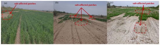
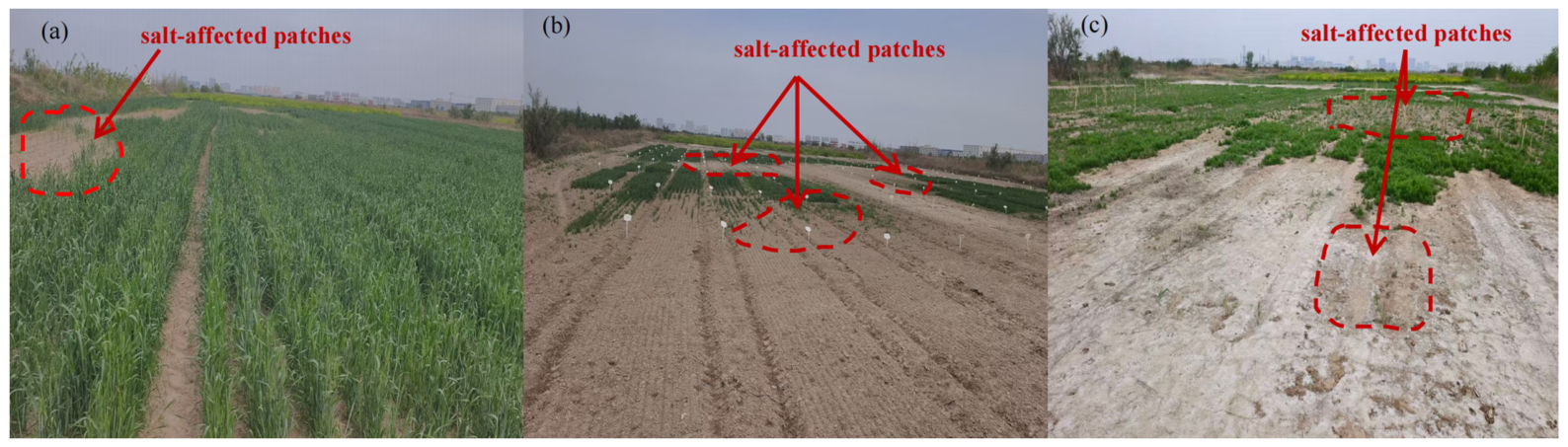
Village-level prediction is closely related to the spatial distribution pattern of salinity in coastal saline–alkali farmland. In this region, soil salinity is not uniformly distributed, but often appears as landscape-scale salt-affected patches [39,40,41]. These patches may occur over several meters to tens of meters and can strongly affect local crop growth. Field observations also confirmed the presence of obvious salt-affected patches within cultivated fields, where areas with visible surface salt accumulation or sparse vegetation showed weaker crop growth than adjacent normally growing areas (Figure 15). Previous studies have shown that soil salinity monitoring is influenced by scale effects, and that medium-resolution satellite-based yield estimation may also be affected by mixed pixels and cropland mask uncertainty [41,42,43]. If the prediction scale is too coarse, such as the county scale, local salt patches and their effects on crop growth may be averaged out, making it difficult to capture local salinity stress signals [41,42,43]. In contrast, if the scale is too small, such as individual experimental plots, the results may depend strongly on specific field conditions and may not represent broader agricultural management units [43]. Therefore, village-level prediction provides a suitable compromise between capturing landscape-scale salinity heterogeneity and supporting practical agricultural management.
Figure 15.
Field observations of salt-affected patches in coastal saline–alkali farmland. (a) Localized weak-growth areas in a wheat field; (b) spatially uneven crop emergence and growth in experimental plots, accompanied by visible salt-affected patches; (c) bare or sparsely vegetated saline patches with evident surface salt accumulation. Red dashed circles indicate representative salt-affected patches.
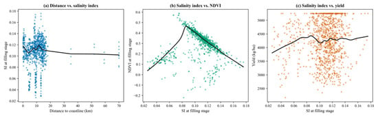
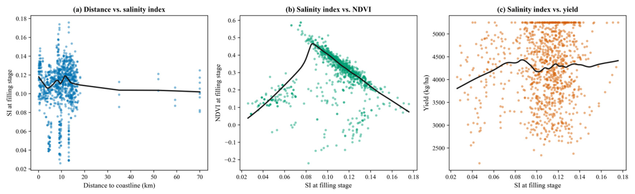
In the absence of field-measured soil electrical conductivity data, the Salinity Index (SI) was used as a salinity proxy, showing a significant negative correlation with NDVI (Spearman r = −0.343, p < 0.001), which supports the interpretation that salinity stress mediates the relationship between coastal proximity and reduced crop yield (Figure 16).
Figure 16.
Salinity Index (SI) as a proxy for salinity mechanism evidence. (a) Distance to coastline vs. SI at filling stage; (b) SI at filling stage vs. NDVI at filling stage; (c) SI at filling stage vs. yield. The LOWESS curves (black lines) show the overall trend in each relationship. Blue points represent the sample relationship between coastline distance and SI, green points represent the relationship between SI and NDVI, and orange points represent the relationship between SI and yield; each point corresponds to one village-level sample.
4.6. Mechanistic Interpretation, Spatial Implications, and Future Work
The spatial prediction maps show that both models captured a stable inland–coastal productivity gradient. Higher-yield areas were mainly distributed in the inland central and southwestern regions, whereas lower-yield areas were concentrated in the eastern coastal zone. This pattern is consistent with spatial differences in salinity stress and water–salt constraints [31,35,36,44,45]. The relatively small mean difference between XGBoost and the Three-Stage Fusion XGBoost Model suggests that the fusion model maintained regional-scale consistency while refining local spatial behavior. In some areas, the fusion model adjusted predictions according to process-related information, such as salinity stress and vegetation growth status, which improved the agronomic interpretation of local yield differences.
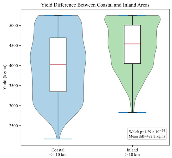
Welch’s t-test confirmed that the yield difference between coastal (mean = 4009.4 kg/ha) and inland areas (mean = 4491.6 kg/ha) was statistically significant (p < 0.001, Cohen’s d = 0.688), with an inland minus coastal mean difference of 482.2 kg/ha (Figure 17). This result indicates that proximity to the coastline is associated with substantially lower winter wheat yield, consistent with the spatial salinity stress gradient in the study area.
Figure 17.
Significance test of yield differences between coastal and inland areas. Violin and box plots show the distribution of village-level yield for coastal (≤10 km from coastline) and inland (>10 km) areas, with Welch’s t-test results and mean difference annotated. The blue violin represents the yield distribution of coastal areas, whereas the green violin represents the yield distribution of inland areas; the white box indicates the interquartile range, the red horizontal line indicates the median, and the black whiskers indicate the whisker range.
SHAP analysis further helped identify key variables and their contribution directions, linking model prediction with agronomic mechanisms [32,35]. For high-dimensional interaction and multi-source fusion models, variable contributions should be interpreted within the context of phenological stages to avoid confusing statistical correlation with causal mechanisms. This is especially important at the village scale, where spatial heterogeneity and management differences are more pronounced [32,34]. The SHAP Dependence Plots (Figure 14) further confirmed that the relationships between key factors and yield are non-linear.
This study still has several limitations. First, although leakage-controlled feature construction was adopted, random stratified splitting may still overestimate cross-spatial transferability under spatial autocorrelation. Future research should evaluate the model using stricter spatial validation strategies, such as spatial block cross-validation or spatial leave-one-out validation. Second, groundwater table data were not included in this study. Incorporating groundwater depth and groundwater salinity information in the future may further improve winter wheat yield prediction in saline–alkali regions.
5. Conclusions
Estimating village-level winter wheat yield in coastal saline–alkali areas remains challenging because of strong spatial heterogeneity and multiple environmental stresses. Using Huanghua City, Hebei Province, as a case study, this study developed a village-scale prediction framework that couples static environmental constraints with dynamic growth responses.
The main conclusions are as follows:
- (1)
- The PGFI-XGBoost branch provided a stable single-stage baseline model for village-level winter wheat yield prediction in coastal saline–alkali farmland, achieving an R2 of 0.6382. Its performance was higher than that of Gradient Boosting (R2 = 0.6256), Random Forest (R2 = 0.6098), SVR (R2 = 0.4792), Ridge regression (R2 = 0.4582), and a single Decision Tree (R2 = 0.3088), indicating that nonlinear ensemble methods are suitable for this village-scale yield prediction task.
- (2)
- After integrating the three-stage branch into the fusion framework, the final predictive performance was improved. The fusion model achieved a Test R2 of 0.6439, an RMSE of 446.24 kg/ha, and an MAE of 363.38 kg/ha, outperforming the single-stage PGFI baseline model under the same data split.
- (3)
- SHAP analysis showed that geospatial factors, such as distance to the coastline and elevation, as well as vegetation growth status indicators, such as NDVI, were important contributors to yield variation. The predicted yield maps showed a clear in-land–coastal gradient, with relatively higher yields in inland areas, approximately 5145 kg/ha, and lower yields in coastal zones, approximately 4198 kg/ha.
- (4)
- At the village scale, the two models produced generally consistent spatial distribution patterns. Relative to the observed mean yield from 2021 to 2023, 4239.06 kg/ha, the mean prediction errors of both models were within 5%, suggesting that the static-constraint and dynamic-driver coupling strategy is feasible for village-scale yield mapping in coastal saline–alkali farmland.
Future research should extend this framework to saline–alkali farmlands across China to further test its applicability and transferability. In addition, groundwater table data in the North China Plain were not included in the current study. Incorporating groundwater depth and groundwater salinity information in the future may further improve the prediction accuracy of winter wheat yield in saline–alkali regions.
Supplementary Materials
The following supporting information can be downloaded at: https://www.mdpi.com/article/10.3390/rs18132233/s1, Dataset S1: Data.csv, village-level multi-source feature dataset used for winter wheat yield prediction.
Author Contributions
Conceptualization, W.J., J.L. and Y.P.; methodology, W.J., J.L. and Y.P.; data curation, W.J.; formal analysis, W.J.; writing—original draft preparation, W.J., Q.Y., Y.X. and X.C.; writing—review and editing, J.L., Y.P., Q.X., Y.Z. (Yapeng Zhou), L.W., X.L., F.Z. and Y.Z. (Yueguo Zhang); supervision, J.L. and Y.P.; project administration, J.L.; funding acquisition, J.L., Y.P. and J.Z. All authors have read and agreed to the published version of the manuscript.
Funding
The APC was funded by the Basic Scientific Research Foundation of Hebei, grant number KY2021024; the Hebei Natural Science Foundation, grant number D2023204017; the Science Research Project of Hebei Education Department, grant number YJZ2024001; the Science and Technology Project of Hebei Education Department, grant number BJ2025143; the Outstanding Postdoctoral Program of Jiangsu Province, grant number 2022ZB506; the Natural Science Foundation of Jiangsu Province, grant number BK20231067; and the Research Fund of Hebei Agricultural University, grant number 3118089.
Data Availability Statement
The original contributions presented in this study are included in the article/Supplementary Materials. Further inquiries can be directed to the corresponding author.
Conflicts of Interest
The authors declare no conflicts of interest.
Abbreviation
The following abbreviation is used in this manuscript:
| PGFI-XGBoost | Phenology-Guided Feature Integration XGBoost |
Appendix A
Figure A1.
Comparison chart of model indices.
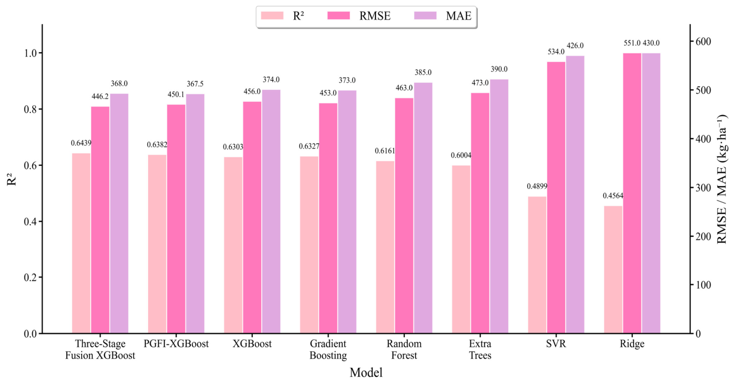
Table A1.
Configurations of PGFI-XGBoost.
Table A2.
Quadrant-based spatial mixing of training and test samples.
References
- Du, M.; Lei, J.; Li, S. Navigating the path to food security in China: Challenges, policies, and future directions. Foods 2025, 14, 644. [Google Scholar] [CrossRef] [Scilit] [PubMed]
- Zheng, J.; Zhang, S. Assessing the impact of climate change on winter wheat production in the North China plain from 1980 to 2020. Agriculture 2025, 15, 449. [Google Scholar] [CrossRef] [Scilit]
- Wang, G.; Ni, G.; Feng, G.; Burrill, H.M.; Li, J.; Zhang, J.; Zhang, F. Saline-alkali soil reclamation and utilization in China: Progress and prospects. Front. Agric. Sci. Eng. 2024, 11, 216–228. [Google Scholar] [CrossRef] [Scilit]
- Gao, H.; Fu, T.; Wang, F.; Zhang, M.; Qi, F.; Liu, J. Influence of groundwater table depth on the evolution of saline-alkali land in a coastal area. Land Degrad. Dev. 2024, 35, 2857–2866. [Google Scholar] [CrossRef] [Scilit]
- Chang, Y.; Zhang, J.; Meng, H.; Li, H. Geospatial assessment of soil salinity–nutrient stratification and soil health responses to groundwater table dynamics in the Bohai Rim region, China. Geomat. Nat. Hazards Risk 2026, 17, 2616998. [Google Scholar] [CrossRef] [Scilit]
- Yuan, J.; Zhang, Y.; Zheng, Z.; Yao, W.; Wang, W.; Guo, L. Grain crop yield prediction using machine learning based on UAV remote sensing: A systematic literature review. Drones 2024, 8, 559. [Google Scholar] [CrossRef] [Scilit]
- Meghraoui, K.; Sebari, I.; Pilz, J.; Ait El Kadi, K.; Bensiali, S. Applied deep learning-based crop yield prediction: A systematic analysis of current developments and potential challenges. Technologies 2024, 12, 43. [Google Scholar] [CrossRef] [Scilit]
- Song, X.P.; Li, H.; Potapov, P.; Hansen, M.C. Annual 30 m soybean yield mapping in Brazil using long-term satellite observations, climate data and machine learning. Agric. For. Meteorol. 2022, 326, 109186. [Google Scholar] [CrossRef] [Scilit]
- Sishodia, R.P.; Ray, R.L.; Singh, S.K. Applications of remote sensing in precision agriculture: A review. Remote Sens. 2020, 12, 3136. [Google Scholar] [CrossRef] [Scilit]
- Zhang, J.; Ge, X.; Hou, X.; Han, L.; Zhang, Z.; Feng, W.; Zhou, Z.; Luo, X. Strategies for soil salinity mapping using remote sensing and machine learning in the Yellow River Delta. Remote Sens. 2025, 17, 2619. [Google Scholar] [CrossRef] [Scilit]
- Farifteh, J. Interference of salt and moisture on soil reflectance spectra. Int. J. Remote Sens. 2011, 32, 8711–8724. [Google Scholar] [CrossRef] [Scilit]
- Van Klompenburg, T.; Kassahun, A.; Catal, C. Crop yield prediction using machine learning: A systematic literature review. Comput. Electron. Agric. 2020, 177, 105709. [Google Scholar] [CrossRef] [Scilit]
- Han, J.; Zhang, Z.; Cao, J.; Luo, Y.; Zhang, L.; Li, Z.; Zhang, J. Prediction of winter wheat yield based on multi-source data and machine learning in China. Remote Sens. 2020, 12, 236. [Google Scholar] [CrossRef] [Scilit]
- Li, H.; Gao, J.; Guo, Y.; Yuan, X.G. Application of XGBoost model and multi-source data for winter wheat yield prediction in Henan Province of China. Big Data Inf. Anal. 2025, 9, 29–47. [Google Scholar] [CrossRef] [Scilit]
- Shariati, S.A.K.; Abbasi, A. Machine learning-based winter wheat yield prediction using multisource data. Agric. Water Manag. 2025, 322, 109951. [Google Scholar] [CrossRef] [Scilit]
- Peng, D.; Cheng, E.; Feng, X.; Hu, J.; Lou, Z.; Zhang, H.; Zhao, B.; Lv, Y.; Peng, H.; Zhang, B. A deep–learning network for wheat yield prediction combining weather forecasts and remote sensing data. Remote Sens. 2024, 16, 3613. [Google Scholar] [CrossRef] [Scilit]
- Lu, C.; Yang, M.; Dong, S.; Liu, Y.; Li, Y.; Pan, Y. Improving Winter Wheat Yield Estimation Under Saline Stress by Integrating Sentinel-2 and Soil Salt Content Using Random Forest. Agriculture 2025, 15, 1544. [Google Scholar] [CrossRef] [Scilit]
- Imamguluyev, R.; Gurbanov, A.; Jabbarov, A.; Hasanova, S.; Rasulova, G.; Karimova, S.; Khalilova, J.; Azizova, R.; Tahirova, L. Fuzzy Logic for Yield Prediction: Enhancing Decision-Making in Agricultural Economics. AGRIS On-Line Pap. Econ. Inform. 2025, 17, 27–36. [Google Scholar] [CrossRef] [Scilit]
- Petropoulos, T.; Benos, L.; Berruto, R.; Miserendino, G.; Marinoudi, V.; Busato, P.; Zisis, C.; Bochtis, D. Interpretable machine learning for legume yield prediction using satellite remote sensing data. Appl. Sci. 2025, 15, 7074. [Google Scholar] [CrossRef] [Scilit]
- Ed-daoudi, R. Interpretable Machine Learning for Multi-Crop Yield Prediction in Semi-Arid Regions: A Hierarchical Approach to Handle Climate Data Sparsity. J. Glob. Innov. Agric. Sci. 2025, 13, 1217–1228. [Google Scholar] [CrossRef] [Scilit]
- Allbed, A.; Kumar, L.; Aldakheel, Y.Y. Assessing soil salinity using soil salinity and vegetation indices derived from IKONOS high-spatial resolution imageries: Applications in a date palm dominated region. Geoderma 2014, 230, 1–8. [Google Scholar] [CrossRef] [Scilit]
- Chandrasekar, K.; Sesha Sai, M.V.R.; Roy, P.S.; Dwevedi, R.S. Land Surface Water Index (LSWI) response to rainfall and NDVI using the MODIS Vegetation Index product. Int. J. Remote Sens. 2010, 31, 3987–4005. [Google Scholar] [CrossRef] [Scilit]
- Huete, A.; Didan, K.; Miura, T.; Rodriguez, E.P.; Gao, X.; Ferreira, L.G. Overview of the radiometric and biophysical performance of the MODIS vegetation indices. Remote Sens. Environ. 2002, 83, 195–213. [Google Scholar] [CrossRef] [Scilit]
- Cao, J.; Zhang, Z.; Luo, Y.; Zhang, L.; Zhang, J.; Li, Z.; Tao, F. Wheat yield predictions at a county and field scale with deep learning, machine learning, and Google Earth Engine. Eur. J. Agron. 2021, 123, 126204. [Google Scholar] [CrossRef] [Scilit]
- Lopresti, M.F.; Di Bella, C.M.; Degioanni, A.J. Relationship between MODIS-NDVI data and wheat yield: A case study in Northern Buenos Aires province, Argentina. Inf. Process. Agric. 2015, 2, 73–84. [Google Scholar] [CrossRef] [Scilit]
- Sörensen, R.; Zinko, U.; Seibert, J. On the calculation of the topographic wetness index: Evaluation of different methods based on field observations. Hydrol. Earth Syst. Sci. 2006, 10, 101–112. [Google Scholar] [CrossRef] [Scilit]
- Chen, S.; Mao, X.; Shang, S. Response and contribution of shallow groundwater to soil water/salt budget and crop growth in layered soils. Agric. Water Manag. 2022, 266, 107574. [Google Scholar] [CrossRef] [Scilit]
- Xue, J.; Su, B. Significant remote sensing vegetation indices: A review of developments and applications. J. Sens. 2017, 2017, 1353691. [Google Scholar] [CrossRef] [Scilit]
- Shabala, S. Learning from halophytes: Physiological basis and strategies to improve abiotic stress tolerance in crops. Ann. Bot. 2013, 112, 1209–1221. [Google Scholar] [CrossRef] [Scilit] [PubMed]
- Brandt, P.; Beyer, F.; Borrmann, P.; Möller, M.; Gerighausen, H. Ensemble learning-based crop yield estimation: A scalable approach for supporting agricultural statistics. GISci. Remote Sens. 2024, 61, 2367808. [Google Scholar] [CrossRef] [Scilit]
- Zhou, W.; Liu, Y.; Ata-Ul-Karim, S.T.; Ge, Q.; Li, X.; Xiao, J. Integrating climate and satellite remote sensing data for predicting county-level wheat yield in China using machine learning methods. Int. J. Appl. Earth Obs. Geoinf. 2022, 111, 102861. [Google Scholar] [CrossRef] [Scilit]
- Muruganantham, P.; Wibowo, S.; Grandhi, S.; Samrat, N.H.; Islam, N. A Systematic Literature Review on Crop Yield Prediction with Deep Learning and Remote Sensing. Remote Sens. 2022, 14, 1990. [Google Scholar] [CrossRef] [Scilit]
- Li, S.; Huang, J.; Xiao, G.; Huang, H.; Sun, Z.; Li, X. Improved Winter Wheat Yield Estimation by Combining Remote Sensing Data, Machine Learning, and Phenological Metrics. Remote Sens. 2024, 16, 3217. [Google Scholar] [CrossRef] [Scilit]
- Joshi, A.; Pradhan, B.; Gite, S.; Chakraborty, S. Remote-Sensing Data and Deep-Learning Techniques in Crop Mapping and Yield Prediction: A Systematic Review. Remote Sens. 2023, 15, 2014. [Google Scholar] [CrossRef] [Scilit]
- Ashfaq, M.; Khan, I.; Alzahrani, A.; Tariq, M.U.; Khan, H.; Ghani, A. Accurate wheat yield prediction using machine learning and climate–NDVI data fusion. IEEE Access 2024, 12, 40947–40961. [Google Scholar] [CrossRef] [Scilit]
- Suaza-Medina, M.E.; Laguna, J.; Béjar, R.; Zarazaga-Soria, F.J.; Lacasta, J. Evaluating the efficiency of NDVI and climatic data in maize harvest prediction using machine learning. Int. J. Digit. Earth 2024, 17, 2359565. [Google Scholar] [CrossRef] [Scilit]
- Katimbo, A.; Rudnick, D.R.; Zhang, J.; Ge, Y.; DeJonge, K.C.; Franz, T.E.; Shi, Y.; Liang, W.Z.; Qiao, X.; Heeren, D.M.; et al. Evaluation of artificial intelligence algorithms with sensor data assimilation in estimating crop evapotranspiration and crop water stress index. Smart Agric. Technol. 2023, 4, 100176. [Google Scholar] [CrossRef] [Scilit]
- John, K.; Saurette, D.D.; Heung, B. The problematic case of data leakage: A case for leave-profile-out cross-validation in 3-dimensional digital soil mapping. Geoderma 2025, 455, 117223. [Google Scholar] [CrossRef] [Scilit]
- Stock, A.; Subramaniam, A. Iterative spatial leave-one-out cross-validation and gap-filling based data augmentation for supervised learning applications in marine remote sensing. GISci. Remote Sens. 2022, 59, 1281–1300. [Google Scholar] [CrossRef] [Scilit]
- Roberts, D.R.; Bahn, V.; Ciuti, S.; Boyce, M.S.; Elith, J.; Guillera-Arroita, G.; Hauenstein, S.; Lahoz-Monfort, J.J.; Schröder, B.; Thuiller, W.; et al. Cross-validation strategies for data with temporal, spatial, hierarchical, or phylogenetic structure. Ecography 2017, 40, 913–929. [Google Scholar] [CrossRef] [Scilit]
- Chen, H.; Wu, J.; Xu, C. Monitoring Soil Salinity Classes through Remote Sensing-Based Ensemble Learning Concept: Considering Scale Effects. Remote Sens. 2024, 16, 642. [Google Scholar] [CrossRef] [Scilit]
- Liu, J.; Shang, J.; Qian, B.; Huffman, T.; Zhang, Y.; Dong, T.; Jing, Q.; Martin, T. Crop Yield Estimation Using Time-Series MODIS Data and the Effects of Cropland Masks in Ontario, Canada. Remote Sens. 2019, 11, 2419. [Google Scholar] [CrossRef] [Scilit]
- Wang, X.; Ma, Y.; Xu, Y.; Huang, Q.; Yang, Z.; Zhang, Z. Learning County from Pixels: Corn Yield Prediction with Attention-Weighted Multiple Instance Learning. Int. J. Remote Sens. 2025, 46, 2815–2845. [Google Scholar] [CrossRef] [Scilit]
- Lobell, D.B.; Sibley, A.; Ortiz-Monasterio, J.I. Extreme heat effects on wheat senescence in India. Nat. Clim. Change 2012, 2, 186–189. [Google Scholar] [CrossRef] [Scilit]
- Raza, A.; Shahid, M.A.; Zaman, M.; Miao, Y.; Huang, Y.; Safdar, M.; Maqbool, S.; Muhammad, N.E. Improving Wheat Yield Prediction with Multi-Source Remote Sensing Data and Machine Learning in Arid Regions. Remote Sens. 2025, 17, 774. [Google Scholar] [CrossRef] [Scilit]

Disclaimer/Publisher’s Note: The statements, opinions and data contained in all publications are solely those of the individual author(s) and contributor(s) and not of MDPI and/or the editor(s). MDPI and/or the editor(s) disclaim responsibility for any injury to people or property resulting from any ideas, methods, instructions or products referred to in the content. |
© 2026 by the authors. Licensee MDPI, Basel, Switzerland. This article is an open access article distributed under the terms and conditions of the Creative Commons Attribution (CC BY) license.