Land-Cover-Stratified Validation and Uncertainty Prioritization for SSP-Based NDVI Projection at 1 km Resolution in Northeast China

Highlights

What are the main findings?

• The study proposes a class-aware framework for SSP-based NDVI projection that integrates projection-oriented model selection, land-cover-stratified validation, uncertainty characterization, and validation-priority ranking.
• Regional NDVI is projected to increase modestly by 2040, but land-cover-stratified validation showed that global model performance masked weak predictive support for Water bodies and Unused land.

What are the implications of the main findings?

• Future NDVI projections should be evaluated beyond global accuracy metrics because aggregate performance can hide important class-level uncertainty and prediction errors.
• The framework identifies Water bodies, Unused land, and Construction land as priority classes for targeted validation, supporting more transparent and reliable interpretation of vegetation projections.

Abstract

At 1 km resolution, NDVI projections for heterogeneous landscapes can appear spatially coherent in aggregate while concealing substantial class-level prediction weaknesses, a limitation that has received limited systematic attention in the NDVI projection literature. This study applies a four-component assessment workflow to Northeast China (NEC) for 2040 under SSP1-2.6, SSP2-4.5, and SSP5-8.5, integrating multi-stage model selection, land-cover-stratified validation, quantile-regression-based uncertainty characterization, and validation-priority ranking. Among three candidate tree-based models evaluated using spatial block cross-validation, temporal holdout validation, long-jump extrapolation, and climatic perturbation tests, LightGBM showed the most balanced and consistent performance, with spatial CV R² = 0.654 ± 0.123, temporal holdout R² = 0.710, and long-jump R² = 0.671, and was therefore selected for the 2040 projection. Projected regional mean NDVI increased modestly from 0.393 in 2020 to 0.414–0.417 across scenarios, with limited divergence among SSP pathways at this near-term horizon. Class-stratified validation of the 2020 holdout prediction revealed that global model performance masked strong class-level heterogeneity, with R² values ranging from 0.576 for Construction land to −0.886 for Unused land. Water bodies and Unused land exhibited negative R² values, indicating weak class-level predictive support relative to a simple class-mean benchmark. Residual decomposition showed that Water bodies combined high random error with elevated systematic deviation, whereas Unused land was mainly characterized by systematic bias, suggesting different needs for class-specific model improvement. The Uncertainty Risk Index (URI), derived from 95% prediction intervals, was highest in Construction land and lowest in Cropland across all scenarios. Integrating historical residuals with future URI-identified Water bodies, Unused land, and Construction land as the highest-priority classes for future targeted validation. These priorities arise from both limited class representation and intrinsic NDVI-related complexity, including low vegetation signal, mixed-pixel effects, and heterogeneous land-surface composition. These results demonstrate that land-cover-stratified error decomposition and uncertainty-informed priority ranking reveal class-specific projection limitations that aggregate accuracy metrics can conceal.

1. Introduction

The Normalized Difference Vegetation Index (NDVI) is a widely used indicator of vegetation greenness and ecosystem productivity, and has been extensively applied to monitor land-surface dynamics under changing climatic and socioeconomic conditions [1]. As a sensitive proxy for photosynthetic activity and biomass, NDVI plays a central role in ecological monitoring by linking climate variability, land-use change, and ecosystem functioning across multiple spatial and temporal scales [2]. China has become a major focus of vegetation change research, with long-term analyses documenting a pronounced greening trend driven by climate warming, precipitation variability, and large-scale ecological restoration programs such as Grain for Green and the Three-North Shelterbelt Program [3,4,5].

Northeast China (NEC) is a critical pillar of national food security, supplying approximately one-third of China’s grain production, and its vegetation dynamics are shaped by a complex interplay of climate forcing, ecological restoration, and rapid urbanization [2,5]. Despite this importance, high-resolution spatially explicit NDVI projection under SSP scenarios remains limited for NEC. Existing studies have mainly been conducted either at coarse national scales or in other regional contexts, such as the Yangtze River Delta and the Yellow River Basin [6,7], which provide useful ecological reference settings for NEC. Moreover, NEC contains diverse land-cover types—including forest, cropland, grassland, and expanding urban areas—making aggregate model validation insufficient, because a model that performs well on average may still fail in the classes most relevant to ecological conservation and land-management decisions.

Machine-learning approaches have demonstrated strong capacity for spatially explicit NDVI modeling, with statistical, tree-based, deep-learning, and hybrid frameworks increasingly applied across scales [6,8,9,10]. Among tree-based methods, LightGBM offers particular advantages for large-scale spatial prediction because of its computational efficiency and ability to capture nonlinear relationships in high-dimensional data [11,12,13]. Recent studies have also begun to project NDVI under SSP-based climate scenarios, showing that vegetation trajectories may diverge across emission pathways when future climate forcing is incorporated into model simulations [14,15,16].

However, a critical and under-addressed methodological limitation persists across the NDVI projection literature: model evaluation is commonly reported using globally or regionally averaged accuracy metrics, with limited attention to land-cover-stratified performance or decomposition of prediction error into systematic and random components. For example, Nguyen et al. [14] projected global NDVI under SSP scenarios using a machine-learning framework and evaluated model performance using aggregate metrics before mapping future NDVI trends. Guo et al. [8] developed an LSTM-based NDVI prediction model for the Yellow River Basin using climate inputs, while Yang et al. [15] projected future vegetation dynamics under SSP/RCP pathways by integrating climate and human-activity drivers. Although these studies provide important advances in future NDVI modeling, none of these studies stratified validation metrics or residual error by land-cover class. Consequently, whether projection performance varies among ecologically and agriculturally important classes—such as cropland, forest, water bodies, unused land, and Construction land—remains insufficiently resolved.

This limitation is particularly consequential in heterogeneous landscapes such as NEC, where cropland, forest, grassland, water bodies, unused land, and expanding construction land coexist within a single regional domain. Existing NDVI projection studies have advanced the assessment of future vegetation dynamics at global, national, and regional scales [6,7,8,14,15,16,17,18]; however, many SSP-based projections remain constrained by coarse climate-grid resolutions, typically around 25–100 km [14,17], or are evaluated mainly using averaged accuracy metrics [14,15] regionally. Such coarse grids are insufficient for resolving the land-cover heterogeneity that controls NDVI responses in NEC, especially across cropland–forest mosaics, urbanizing areas, wetlands, and marginal unused land. In this context, harmonizing predictors to a 1 km grid provides a more operational spatial scale for linking projected vegetation change with cropland distribution, forest systems, urban expansion, and ecological protection zones. Therefore, a 1 km SSP-based NDVI projection offers practical value beyond regional mean trend assessment by supporting land-cover-stratified validation and spatial prioritization of classes with higher projection uncertainty.

Furthermore, projecting NDVI under SSP scenarios requires not only future climatic forcing, but also scenario-consistent land cover and socioeconomic inputs. In this study, GDP and population density were incorporated as part of the broader predictor framework to improve consistency between historical model development and future scenario-based projection, consistent with prior work linking socioeconomic drivers to land-surface vegetation dynamics [3,4]. To the best of our knowledge, few previous studies have combined land-cover-stratified error decomposition, quantile-regression-based uncertainty characterization, and validation-oriented prioritization within a high-resolution SSP-based NDVI projection framework for NEC. This highlights an important methodological gap in class-level NDVI projection assessment. The three SSP scenarios used in this study represent contrasting socioeconomic and climate-forcing pathways. SSP1-2.6 describes a sustainability-oriented, low-forcing pathway; SSP2-4.5 represents an intermediate “middle-of-the-road” pathway; and SSP5-8.5 represents a high-forcing pathway associated with fossil-fuel-based development. These scenarios were selected to represent low, moderate, and high climate-pressure conditions for evaluating the proposed class-aware NDVI projection framework [19,20]. SSP3-7.0 was not included because the objective was not to compare all CMIP6 pathways, but to evaluate the proposed class-aware validation framework under three contrasting low-, intermediate-, and high-forcing conditions represented by SSP1-2.6, SSP2-4.5, and SSP5-8.5.

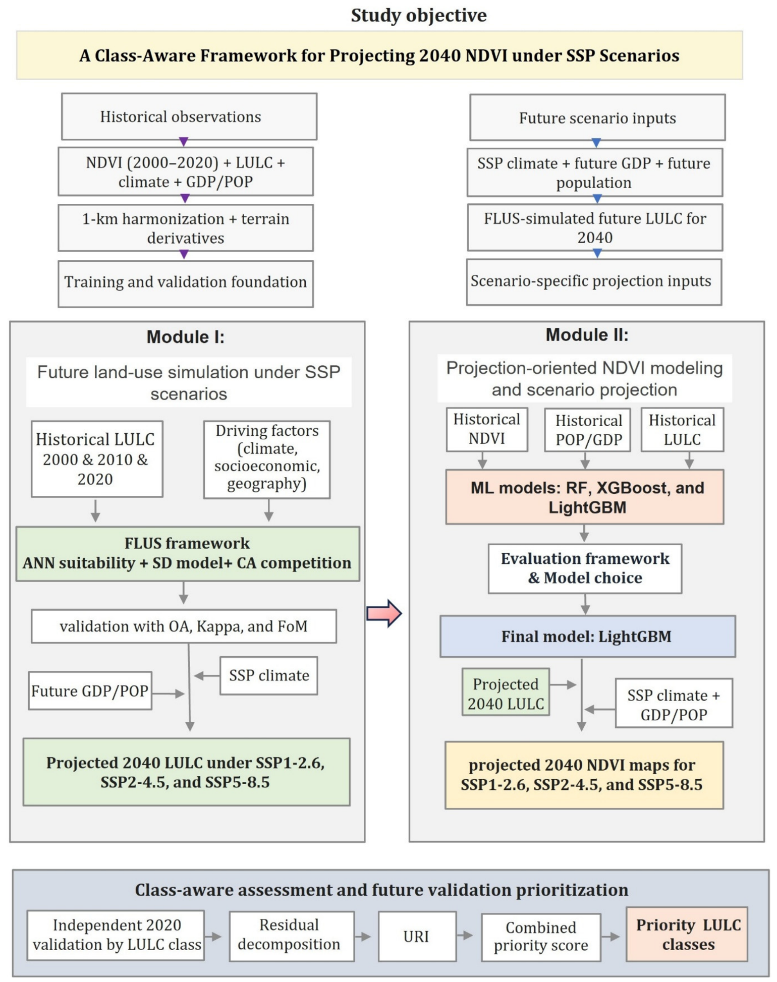
This study aimed to develop and apply a class-aware framework for projecting and assessing 1 km NDVI in Northeast China for 2040 under SSP1-2.6, SSP2-4.5, and SSP5-8.5. Unlike conventional NDVI projection studies that mainly report overall accuracy or scenario-level mean changes, the proposed framework evaluates how projection reliability varies among land-cover classes. Specifically, it integrates four linked components: (1) projection-oriented model selection using spatial, temporal, extrapolation, and climate-perturbation tests; (2) land-cover-stratified validation using systematic and random error decomposition; (3) relative projection uncertainty assessment using a quantile-regression-based Uncertainty Risk Index (URI); and (4) validation-priority ranking that combines historical error structure with future uncertainty. Together, these components evaluate where projected NDVI patterns are reliably supported and where additional validation effort is most needed.

2. Study Area and Methods

2.1. Study Area

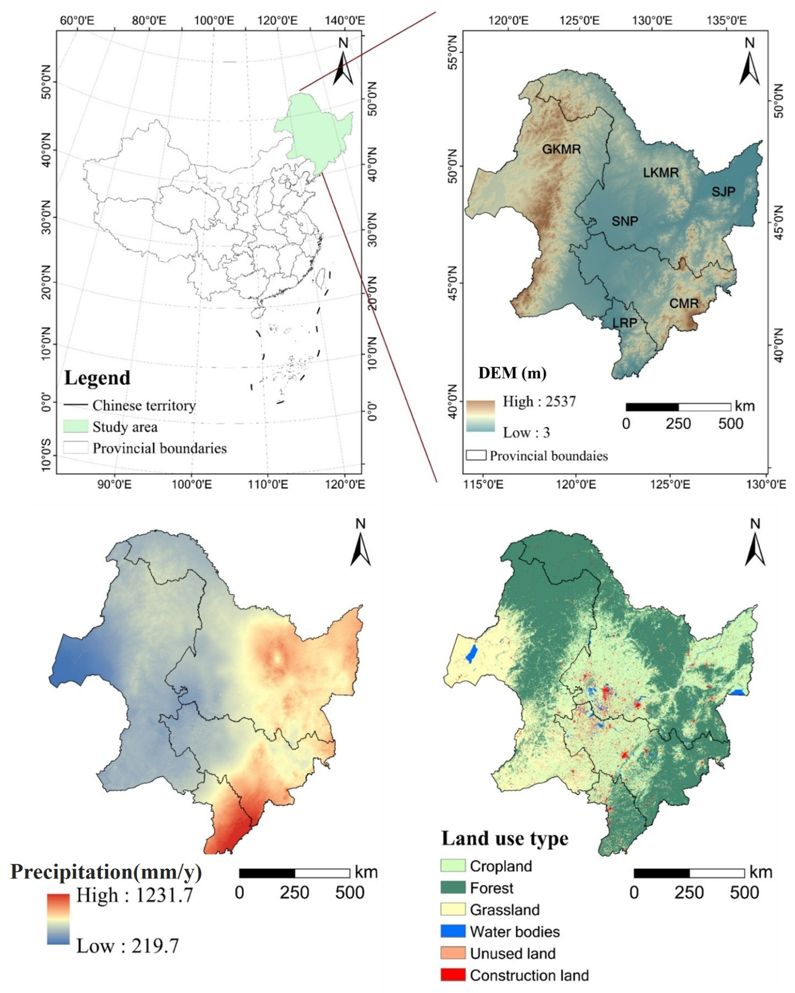
Northeast China (NEC), spanning over 1 million km², includes the provinces of Heilongjiang, Jilin, Liaoning, and the Inner Mongolia Autonomous Region. The region features mountains along its western, northern, and eastern borders, with flat plains dominating the interior (Figure 1). NEC has a temperate continental monsoonal climate with mean annual precipitation of 400–700 mm and mean annual temperature of −1.1 °C to 4.4 °C [21], and it supplies approximately one-third of China’s grain products and serves as a critical pillar of national food security. However, vegetation dynamics in NEC are shaped by a complex interplay of climate forcing, ecological restoration, and rapid urbanization [4], creating a spatially heterogeneous NDVI landscape [22] that makes NEC an ideal but analytically demanding case for high-resolution vegetation projection under future climate scenarios.

2.2. Study Design and Overall Framework

This study was designed not only to project the spatial distribution of NDVI at 1 km resolution for 2040 under alternative socio-climatic scenarios (SSP1-2.6, SSP2-4.5, and SSP5-8.5), but also to assess those projections through a stratified validation workflow tailored to heterogeneous landscapes. The 2040 projection horizon was selected as a near-term future period because it is relevant for regional ecological planning, agricultural management, and land-use policy, while avoiding some of the larger uncertainties associated with late-century projections. In this study, the 2040 climate input is represented by the WorldClim v2.1 CMIP6 near-term 20-year average for 2021–2040, which is the closest available future climate time slice to the selected projection horizon. The overall methodological workflow is summarized in Figure 2.

MODIS NDVI was derived from the MOD13A1 Collection 6.1 product accessed through Google Earth Engine, which provides 16-day vegetation index composites at 500 m spatial resolution. For 2000–2020, the 16-day NDVI composites were aggregated into annual median NDVI to reduce the influence of residual cloud contamination, atmospheric noise, and extreme observations. Temporal consistency was maintained by pairing each annual NDVI layer with predictor layers from the same year; monthly temperature and precipitation data were converted to annual mean temperature and annual total precipitation, respectively, while annual LULC, GDP, and population layers were matched by year. For the 2040 projection, WorldClim CMIP6 tn, tx, and pr variables were converted to the same annual climate definitions used for historical modeling. All annual layers were harmonized to the common 1 km × 1 km modeling grid, and detailed dataset information is provided in

Table 1. Input datasets used for historical NDVI modeling and 2040 scenario-based projection in Northeast China.

Variable	Product/Source	Spatial Resolution	Temporal Period Used	Role
Land use/land cover (LULC)	China’s 30 m annual land-cover dataset and its dynamic changes, NCDC/Zenodo	30 m	2000–2020	Predictor for SHAP, NDVI projection, and LULC projection
Air temperature (TEMP)	1 km monthly mean temperature dataset for China, TPDC	1 km	2000–2020	Predictor for SHAP, NDVI projection, and LULC projection
Precipitation (PRE)	1 km monthly precipitation dataset for China, TPDC	1 km	2000–2020	Predictor for SHAP, NDVI projection, and LULC projection
Normalized Difference Vegetation Index (NDVI)	MODIS MOD13A1 Collection 6.1, Google Earth Engine	500 m	2000–2020	Response variable
Gross Domestic Product (GDP)	Annual gridded GDP dataset, Wang and Sun	1 km	2000–2020	Predictor for SHAP, NDVI projection, and LULC projection
Population density (POP)	WorldPop annual gridded population dataset	1 km	2000–2020	Predictor for SHAP, NDVI projection, and LULC projection
Distance to road	Road-distance raster dataset, RESDC	1 km	Static	Predictor for LULC projection
Distance to water	Water-distance raster dataset, RESDC	1 km	Static	Predictor for SHAP, NDVI projection, and LULC projection
Digital Elevation Model (DEM)	Shuttle Radar Topography Mission (SRTM) DEM	90 m	Static	Predictor for SHAP, NDVI projection, and LULC projection
Slope	Derived from SRTM DEM	90 m	Static	Predictor for SHAP, NDVI projection, and LULC projection
Topographic Wetness Index (TWI)	Derived from SRTM DEM	90 m	Static	Predictor for SHAP, NDVI projection, and LULC projection
Future land use/land cover	FLUS-simulated LULC scenario maps	1 km	2040	Predictor for NDVI projection
Future air temperature	WorldClim v2.1 downscaled CMIP6	1 km	2021–2040 time slice, used as 2040 input	Predictor for FLUS and NDVI projection
Future precipitation	WorldClim v2.1 downscaled CMIP6	1 km	2021–2040 time slice, used as 2040 input	Predictor for FLUS and NDVI projection
Future GDP	Science Data Bank SSP1–5_v2 gridded GDP dataset	1 km	2040	Predictor for FLUS and NDVI projection
Future population density	WorldPop/University of Southampton SSP population projection dataset	30 arc-seconds (1 km)	2040	Predictor for FLUS and NDVI projection

Note: Full dataset metadata, including product versions, DOI/URL information, access period, temporal resolution, and temporal harmonization, are provided in Table S12.

.

2.2.1. Simulation of Future Land Use/Land Cover

Future LULC maps for 2040 under SSP scenarios were generated using the Future Land-Use Simulation (FLUS) model. FLUS simulates the spatial trajectories of multiple land-use/land-cover changes by coupling a top-down system dynamics (SD) module with a bottom-up cellular automata (CA) module, allowing macro-level land-demand changes and local spatial competition among land-cover types to be represented simultaneously [23]. Within this framework, the ANN suitability module estimates the probability of land-cover transitions, while adaptive inertia coefficients, neighborhood effects, conversion costs, and a roulette selection mechanism regulate the spatial allocation of land-cover changes [24,25,26].

In the CA allocation stage, a land-use conversion cost matrix, neighborhood weights, and iterative allocation rules were defined to control spatial simulation. The conversion cost matrix specified permitted and restricted transitions among land-cover classes, whereas neighborhood weights controlled the influence of surrounding land-cover composition on class expansion probability. The FLUS-CA allocation process was conducted using up to 100 iterations, with the simulation terminating when the predefined 2040 land-demand target was reached or when allocation convergence occurred. The conversion cost matrix and neighborhood weights are provided in Tables S1 and S2. Neighborhood weights are dimensionless, class-specific FLUS calibration parameters bounded between 0 and 1, where higher values indicate stronger neighborhood-driven expansion tendency [23]. The weights in Table S1 were locally assigned for this study by expert judgment to reflect class-specific development pressure, spatial constraints, and expansion potential. This parameterization follows FLUS/CA-based calibration practice, in which neighborhood weights are locally specified and evaluated through historical validation against the observed 2010 and 2020 LULC maps [23,27].

The FLUS suitability module was calibrated using historical LULC transitions during 2000–2020, and the associated driving factors, and the simulation performance was validated by comparing simulated and observed LULC maps for 2010 and 2020. Validation accuracy was assessed using overall accuracy (OA), Kappa coefficient, and Figure of Merit (FoM) [27]. After satisfactory validation performance was achieved, the calibrated FLUS parameters were applied to simulate 2040 LULC under SSP1-2.6, SSP2-4.5, and SSP5-8.5 using scenario-specific climatic and socioeconomic inputs. Input data sources are summarized in Table 1. The 2040 land-demand target was derived from the observed 2000–2020 LULC transition trajectory using CA-Markov and used as a fixed-demand input for all FLUS-CA scenario allocations. In this implementation, the SD module was not used to impose separate policy-driven demand assumptions for each SSP scenario. This controlled-demand design was used to separate demand-side effects from allocation-side effects; therefore, differences among SSP LULC outputs reflect scenario-specific climate, GDP, and population suitability inputs rather than separate land-demand vectors.

Future precipitation and temperature data were obtained from WorldClim v2.1 downscaled CMIP6 products for the near-term 2021–2040 period, which was used to represent 2040 climatic conditions, at 0.0083333° (~1 km) resolution [28]. These products are calibrated using WorldClim v2.1 as the baseline climate. Five CMIP6 GCMs were selected for each SSP scenario based on their use in previous CMIP6-based vegetation and climate-impact studies, complete availability for SSP1-2.6, SSP2-4.5, and SSP5-8.5 in WorldClim v2.1, and full spatial coverage of the NEC domain [15,17,29]. Table S3 summarizes the native resolutions of the five GCMs used in this study. For each climate variable and SSP scenario, the five downscaled GCM rasters were checked and aligned to ensure consistent projection, extent, resolution, and pixel alignment. A pixel-wise multi-model ensemble mean (MME) was then calculated using ArcGIS Raster Calculator to reduce dependence on any individual GCM and provide a representative 2040 climate signal for LULC simulation and NDVI projection [30]. The resulting climate grids were clipped to the NEC boundary and used as inputs for the 2040 LULC simulation and NDVI projection.

Future socioeconomic inputs were obtained from SSP-consistent gridded products rather than downscaled independently in this study. Future GDP data for 2040 were obtained from the Science Data Bank dataset “Global and China population and economy gridded datasets under Shared Socioeconomic Pathways (SSP1–5)_v2” [31]. Future population data for 2040 were obtained from the WorldPop/University of Southampton dataset “Global 1km-grid population projections for 2025–2100 consistent with the Shared Socioeconomic Pathways 3.2 national population projections, version 0.2” [32]. For scenario consistency, the SSP1, SSP2, and SSP5 socioeconomic layers were matched with SSP1-2.6, SSP2-4.5, and SSP5-8.5, respectively. Both socioeconomic products were already provided as gridded SSP-based layers at approximately 1 km spatial resolution; therefore, no independent GDP or population downscaling was performed. The GDP and population rasters were reprojected, clipped to the NEC boundary, and aligned to the common 1 km modeling grid before being used as inputs for the 2040 FLUS and subsequent NDVI projection. Regional 2040 socioeconomic summaries derived from the final aligned rasters are reported in Table S11.

LULC Allocation Uncertainty Assessment

To evaluate the sensitivity of future LULC allocation to uncertainty in key FLUS allocation parameters, ten additional perturbation runs were generated for each SSP scenario. In these runs, neighborhood weights and acceleration-related parameters varied within ±5% of their calibrated values as a controlled local sensitivity test, while preserving the relative ranking among land-cover classes. The original FLUS-simulated LULC raster was retained as the official scenario-specific projection, whereas the perturbation realizations were used only to characterize spatial allocation instability.

For each pixel, class occurrence probabilities were calculated across the original and perturbation-based realizations. Three indicators were derived: stability probability, defined as the maximum class occurrence probability; variation uncertainty, defined as one minus the maximum class occurrence probability; and normalized Shannon entropy, representing the dispersion of class probabilities across LULC categories.

Class-level uncertainty statistics were summarized using the original FLUS class masks rather than perturbation-derived class assignments, ensuring that instability was assessed relative to the official scenario-specific LULC classes used in the NDVI model. The resulting LULC uncertainty products were interpreted as relative spatial allocation instability indicators, not as fully calibrated probabilistic projections or full propagation of LULC uncertainty into NDVI prediction.

2.2.2. Machine Learning—LightGBM

LightGBM (Light Gradient Boosting Machine) is an efficient gradient boosting framework based on histogram-based, leaf-wise tree growth, and is well-suited for large-scale pixel-wise NDVI modeling [11,13]. Following model comparison, LightGBM was retained as the final model for the 2040 NDVI projection. The predefined parameter settings used for model implementation are reported in Table S4. The final LightGBM model was retrained using the full historical record and then applied to scenario-specific predictor layers to generate spatially explicit NDVI projections for 2040 under SSP1-2.6, SSP2-4.5, and SSP5-8.5.

To improve model interpretability, SHapley Additive ExPlanations (SHAP) was applied to quantify the contribution of each predictor to the model output [33,34]. This approach provides a transparent and consistent basis for identifying the main drivers of NDVI variability.

2.2.3. NDVI Model Construction and Projection

NDVI was modeled using three tree-based machine-learning regression algorithms—Random Forest (RF), XGBoost, and LightGBM—to compare their suitability for forward NDVI projection under heterogeneous land-cover conditions. Historical NDVI observations derived from MODIS at 500 m resolution for 2000–2020 served as the response variable, while the predictor set included land use/land cover (LULC), precipitation (PRE), air temperature (TEMP), population density (POP), gross domestic product (GDP), and static topographic variables, including elevation (DEM), slope, topographic wetness index (TWI), and distance to water (DIST). GDP and population density were included as SSP-consistency socioeconomic covariates and were not interpreted as direct causal ecological drivers of NDVI. All predictor layers were harmonized to a common 1 km grid before model development. Topographic derivatives, including slope and TWI, were derived from the DEM before resampling. Variable selection was performed using the Variance Inflation Factor criterion (VIF < 5) to reduce multicollinearity (Figure S1). The NDVI prediction model can be expressed as:

$${\mathrm{N}\mathrm{D}\mathrm{V}\mathrm{I}}_{(\mathrm{i},\mathrm{t})}=\mathrm{f}{(\mathrm{LULC}}_{\left(\mathrm{i},\mathrm{t}\right)},{\mathrm{PRE}}_{(\mathrm{i},\mathrm{t})},{\mathrm{TEMP}}_{(\mathrm{i},\mathrm{t})},{\mathrm{POP}}_{(\mathrm{i},\mathrm{t})},{\mathrm{GDP}}_{(\mathrm{i},\mathrm{t})},{\mathrm{DEM}}_{(\mathrm{i},\mathrm{t})},{\mathrm{SLOPE}}_{(\mathrm{i},\mathrm{t})},{\mathrm{TWI}}_{(\mathrm{i},\mathrm{t})},{\mathrm{DIST}}_{(\mathrm{i},\mathrm{t})})$$

(1)

where ${\mathrm{N}\mathrm{D}\mathrm{V}\mathrm{I}}_{\left(\mathrm{i},\mathrm{t}\right)}$ denotes the predicted NDVI value for pixel (i) at time (t), and (f) represents the regression function learned by the ML algorithm.

Model comparison was conducted using a multi-stage evaluation framework designed to assess both predictive accuracy and projection-oriented robustness. Three tree-based machine-learning models, Random Forest (RF), LightGBM, and XGBoost, were evaluated using the same predictor set. The predefined hyperparameter settings for all candidate models are provided in Table S4.

First, a temporal validation test was performed by training each candidate model on annual observations from 2000 to 2019 and predicting NDVI for 2020. This step was used to evaluate short-gap temporal transferability under an independent holdout year. Second, a long-horizon extrapolation test was conducted by training each model on 2000–2010 only and then predicting NDVI for 2020, thereby assessing model stability under a substantially larger temporal gap. Third, a climate-perturbation robustness test was applied to compare model behavior under pseudo-novel climatic forcing. In this test, precipitation was increased by 2.5%, temperature was increased by 0.32 °C, and a combined PRE + TEMP perturbation was also applied to the 2020 holdout feature set on a pixel-by-pixel basis. These perturbation values were derived as ensemble-mean CMIP6 projected changes for NEC between 2020 and 2040, calculated from the five GCMs used in this study (Table S3). This experiment was not intended as a formal validation against observations, but rather as a controlled robustness test to assess whether candidate models preserved plausible spatial variability under future-like climatic shifts.

Spatial block cross-validation was implemented using a 5 × 5 spatial blocking scheme, in which the NEC region was divided into 25 spatial blocks that were grouped into five validation folds to reduce spatial autocorrelation between training and validation samples. The NEC raster extent used for spatial block cross-validation was approximately 1554.0 km × 1608.0 km; therefore, the main 5 × 5 spatial blocking scheme corresponded to an approximate block size of 310.8 km × 321.6 km. To assess the block-size effect, spatial block validation was additionally repeated using a coarser 4 × 4 blocking scheme, corresponding to an approximate block size of 388.5 km × 402.0 km. The 4 × 4 scheme produced lower R² and higher RMSE than the 5 × 5 scheme, indicating that the spatial cross-validation results were sensitive to block size (Table S9).

Model selection was based on the combined evidence from these evaluation stages rather than on a single metric. Thus, model comparison was treated as a projection-oriented assessment step, with emphasis on performance consistency under temporal transfer, longer-horizon extrapolation, and future-like climatic perturbation. Under this framework, LightGBM was retained as the final model for 2040 NDVI projection and retrained using the full historical record before being applied to scenario-specific predictor layers to generate spatially explicit NDVI projections for 2040 under SSP1-2.6, SSP2-4.5, and SSP5-8.5. The original scenario-specific FLUS LULC rasters were used as categorical LULC inputs in the main NDVI projections, while the perturbation-derived LULC uncertainty products were retained for robustness assessment and validation-priority analysis.

2.2.4. Stratified Accuracy Assessment and Residual Analysis

Model performance was evaluated using a stratified validation framework based on the independent 2020 holdout prediction generated during the primary temporal validation stage (training in 2000–2019 and predicting 2020). For each LULC class, prediction accuracy was quantified using four complementary metrics: coefficient of determination (R²), Root Mean Square Error (RMSE), Mean Absolute Error (MAE), and prediction bias. All metrics were computed exclusively on spatially coincident valid pixels—pixels with valid values in observed NDVI, predicted NDVI, and LULC layers simultaneously (Equations (2)–(5)):

$${\mathrm{R}}^2=1-{\displaystyle \frac{\frac{1}{\mathrm{n}}{\displaystyle {\sum }_{\mathrm{i}=1}^{\mathrm{n}}}{{(\hat{\mathrm{y}}}_{\mathrm{i}}-{\mathrm{y}}_{\mathrm{i}})}^2}{\frac{1}{\mathrm{n}}{\displaystyle {\sum }_{\mathrm{i}=1}^{\mathrm{n}}}{{(\mathrm{y}}_{\mathrm{i}}-\stackrel{-}{\mathrm{y}})}^2}}$$

(2)

$$\mathrm{R}\mathrm{M}\mathrm{S}\mathrm{E}=\sqrt{{\displaystyle \frac{1}{\mathrm{n}}}{\displaystyle \sum _{\mathrm{i}=1}^{\mathrm{n}}}{{(\hat{\mathrm{y}}}_{\mathrm{i}}-{\mathrm{y}}_{\mathrm{i}})}^2}$$

(3)

$$\mathrm{M}\mathrm{A}\mathrm{E}={\displaystyle \frac{1}{\mathrm{n}}}{\displaystyle \sum _{\mathrm{i}=1}^{\mathrm{n}}}\left|{\hat{\mathrm{y}}}_{\mathrm{i}}-{\mathrm{y}}_{\mathrm{i}}\right|$$

(4)

$$\mathrm{B}\mathrm{i}\mathrm{a}\mathrm{s}={\displaystyle \frac{1}{\mathrm{n}}}{\displaystyle \sum _{\mathrm{i}=1}^{\mathrm{n}}}{(\mathrm{y}}_{\mathrm{i}}-{\hat{\mathrm{y}}}_{\mathrm{i}})$$

(5)

Residual maps were computed as Residual = NDVI Observed—NDVI Predicted, where positive values indicate underprediction and negative values indicate overprediction. Prediction errors were further decomposed into systematic error (|residual mean| = directional bias, correctable) and random error (residual STD = unpredictable spatial scatter, model-structural) [35].

2.2.5. Uncertainty Characterization and Uncertainty Risk Index (URI)

Prediction uncertainty in NDVI predictions was quantified by training three LightGBM quantile regression models at α = 0.025, 0.500, and 0.975 using the pinball loss function [11,36], resulting in a 95% pixel-wise prediction interval whose width was used as input for constructing the URI. In the present study, URI is interpreted primarily as a relative uncertainty indicator derived from interval width, enabling spatial and class-wise comparison of uncertainty patterns rather than serving as a fully calibrated probabilistic risk estimate. Because the quantile models are trained on the same historical data as the main LightGBM model, URI reflects extrapolated model uncertainty rather than fully independent probabilistic bounds. To facilitate spatial comparison, CI width was transformed into the Uncertainty Risk Index (URI) via min–max normalization:

$${\mathrm{URI}}_{\mathrm{i}}={\displaystyle \frac{\mathrm{C}{\mathrm{I}}_{\mathrm{i}}^{95\%}-\mathrm{C}{\mathrm{I}}_{\mathrm{m}\mathrm{i}\mathrm{n}}}{\mathrm{C}{\mathrm{I}}_{\mathrm{m}\mathrm{a}\mathrm{x}}-\mathrm{C}{\mathrm{I}}_{\mathrm{m}\mathrm{i}\mathrm{n}}}}$$

(6)

where $\mathrm{C}{\mathrm{I}}_{\mathrm{i}}^{95\%}$ is the 95% CI width of NDVI prediction at pixel $\mathrm{i}$, and $\mathrm{C}{\mathrm{I}}_{\mathrm{m}\mathrm{i}\mathrm{n}}$ and $\mathrm{C}{\mathrm{I}}_{\mathrm{m}\mathrm{a}\mathrm{x}}$ denote the minimum and maximum CI widths across the study area.

URI ranges from 0 (lowest uncertainty) to 1 (highest uncertainty). URI was extracted per LULC class under SSP1-2.6, SSP2-4.5, and SSP5-8.5 to contextualize historical prediction errors within future climate scenarios. A single study-area-wide min–max normalization was used to construct URI because the objective was to compare relative uncertainty among land-cover classes on a common scale. Class-specific normalization was not used because it would rescale each land-cover class independently and could remove meaningful between-class differences in prediction interval width, which are central to the validation-priority framework.

2.2.6. Combined Priority Score for Future Validation

To identify land-cover types requiring prioritized validation in future studies, a combined priority score was derived by integrating three normalized components: systematic error (weight = 0.4), random error (weight = 0.4), and mean URI across all SSP scenarios (weight = 0.2):

$$\begin{array}{ll}\mathrm{P}\mathrm{r}\mathrm{i}\mathrm{o}\mathrm{r}\mathrm{i}\mathrm{t}\mathrm{y}\mathrm{S}\mathrm{c}\mathrm{o}\mathrm{r}\mathrm{e}=& 0.4\times \mathrm{N}\mathrm{o}\mathrm{r}\mathrm{m}\left(\mathrm{S}\mathrm{y}\mathrm{s}\mathrm{t}\mathrm{e}\mathrm{m}\mathrm{a}\mathrm{t}\mathrm{i}\mathrm{c}\right)+0.4\times \mathrm{N}\mathrm{o}\mathrm{r}\mathrm{m}\left(\mathrm{R}\mathrm{a}\mathrm{n}\mathrm{d}\mathrm{o}\mathrm{m}\right)\\ & +0.2\times \mathrm{N}\mathrm{o}\mathrm{r}\mathrm{m}(\mathrm{U}\mathrm{R}\mathrm{I}\_\mathrm{m}\mathrm{e}\mathrm{a}\mathrm{n})\end{array}$$

(7)

where Norm (Systematic) denotes the normalized absolute mean residual, Norm (Random) denotes the normalized residual standard deviation, and Norm (URI Mean) denotes the normalized mean URI across SSP scenarios.

Since |residual mean|, residual STD, and $\mathrm{U}\mathrm{R}\mathrm{I}\_\mathrm{m}\mathrm{e}\mathrm{a}\mathrm{n}$ operate on fundamentally different numerical scales—with URI range = 0.36 exceeding systematic error range = 0.017 by more than 20-fold—direct aggregation without normalization would allow URI to dominate the composite score regardless of the assigned weight. Min–max normalization was therefore applied independently to each component prior to weighted aggregation, rescaling all inputs to [0, 1] and ensuring that the 0.4/0.4/0.2 weights reflect the intended relative contributions of historical systematic error, historical random error, and future prediction uncertainty, respectively. Higher scores indicate land-cover classes requiring relatively greater validation attention because of the combined influence of historical model error and future projected uncertainty.

Historical error components (systematic and random) were collectively assigned a higher weight (0.8) than future URI (0.2) because they are directly measurable, model-attributable, and actionable through model improvement, whereas URI is partially driven by input uncertainty external to the model. Sensitivity analysis across four weighting schemes—original weight (0.4/0.4/0.2), equal weight (0.33/0.33/0.33), URI-heavy (0.3/0.3/0.4), and history-heavy (0.5/0.4/0.1) confirmed that Water bodies ranked first and Cropland ranked last under all schemes, demonstrating that the priority extremes were robust to weighting assumptions (Table 6).

2.2.7. Supplementary LAII-Informed Robustness Analysis

As an additional robustness test, a LULC Allocation Instability Index (LAII) was incorporated into the validation-priority framework to evaluate whether class-level priorities were sensitive to uncertainty in future land-cover allocation. LAII was derived from controlled LULC-weight perturbation runs. For each pixel, class occurrence probabilities were calculated across perturbation realizations, and variation uncertainty was defined as one minus the maximum class occurrence probability. For each land-cover class, LAII was calculated as the mean class-level variation uncertainty across SSP1-2.6, SSP2-4.5, and SSP5-8.5.

LAII was min–max normalized across land-cover classes and added as a fourth component in a supplementary priority score:

$$\begin{gathered} \mathrm{P}\mathrm{r}\mathrm{i}\mathrm{o}\mathrm{r}\mathrm{i}\mathrm{t}\mathrm{y}\mathrm{S}\mathrm{c}\mathrm{o}\mathrm{r}\mathrm{e}\_\mathrm{L}\mathrm{A}\mathrm{I}\mathrm{I}=0.35\times \mathrm{n}\mathrm{o}\mathrm{r}\mathrm{m}\left(\mathrm{S}\mathrm{y}\mathrm{s}\mathrm{t}\mathrm{e}\mathrm{m}\mathrm{a}\mathrm{t}\mathrm{i}\mathrm{c}\right)+0.35\times \mathrm{n}\mathrm{o}\mathrm{r}\mathrm{m}\left(\mathrm{R}\mathrm{a}\mathrm{n}\mathrm{d}\mathrm{o}\mathrm{m}\right)+0.2\times \mathrm{n}\mathrm{o}\mathrm{r}\mathrm{m}(\mathrm{U}\mathrm{R}\mathrm{I}\_\mathrm{m}\mathrm{e}\mathrm{a}\mathrm{n})+ \\ 0.10\times \mathrm{N}\mathrm{o}\mathrm{r}\mathrm{m}\left(\mathrm{L}\mathrm{A}\mathrm{I}\mathrm{I}\right) \end{gathered}$$

(8)

where Norm (LAII) denotes the min–max normalized LULC Allocation Instability Index.

The original three-component score was retained as the main result because systematic and random errors are directly observed from historical validation, whereas URI and LAII represent relative future uncertainty indicators. The LAII-informed score was therefore used only as a robustness analysis to test whether the validation-priority ranking changed after accounting for LULC allocation instability. This analysis did not modify the URI calculation and did not represent full propagation of LULC uncertainty into NDVI prediction.

3. Results

3.1. Land-Use/Land-Cover Dynamics

3.1.1. Historical Land-Use Changes (2000–2020)

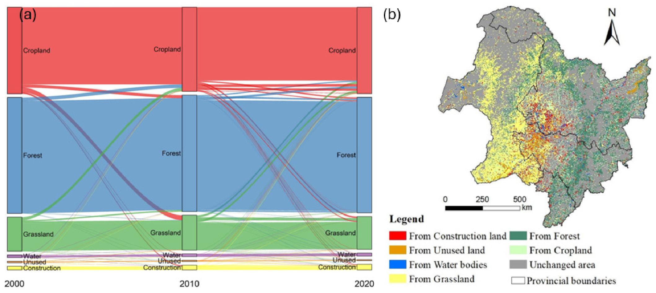
Land-use change from 2000 to 2020 is characterized by strong persistence of forest and cropland, as indicated by the dominant unchanged flows in the Sankey diagram (Figure 3a) and the large diagonal values in the transfer matrix (Table S10). Most transitions occur among cropland, grassland, and Forest, while Construction land expands mainly through conversion from cropland. Spatially, these changes are localized, with unchanged areas dominating the landscape (Figure 3b), indicating overall land-use stability during the study period.

3.1.2. FLUS Model Validation and Projected LULC for 2040

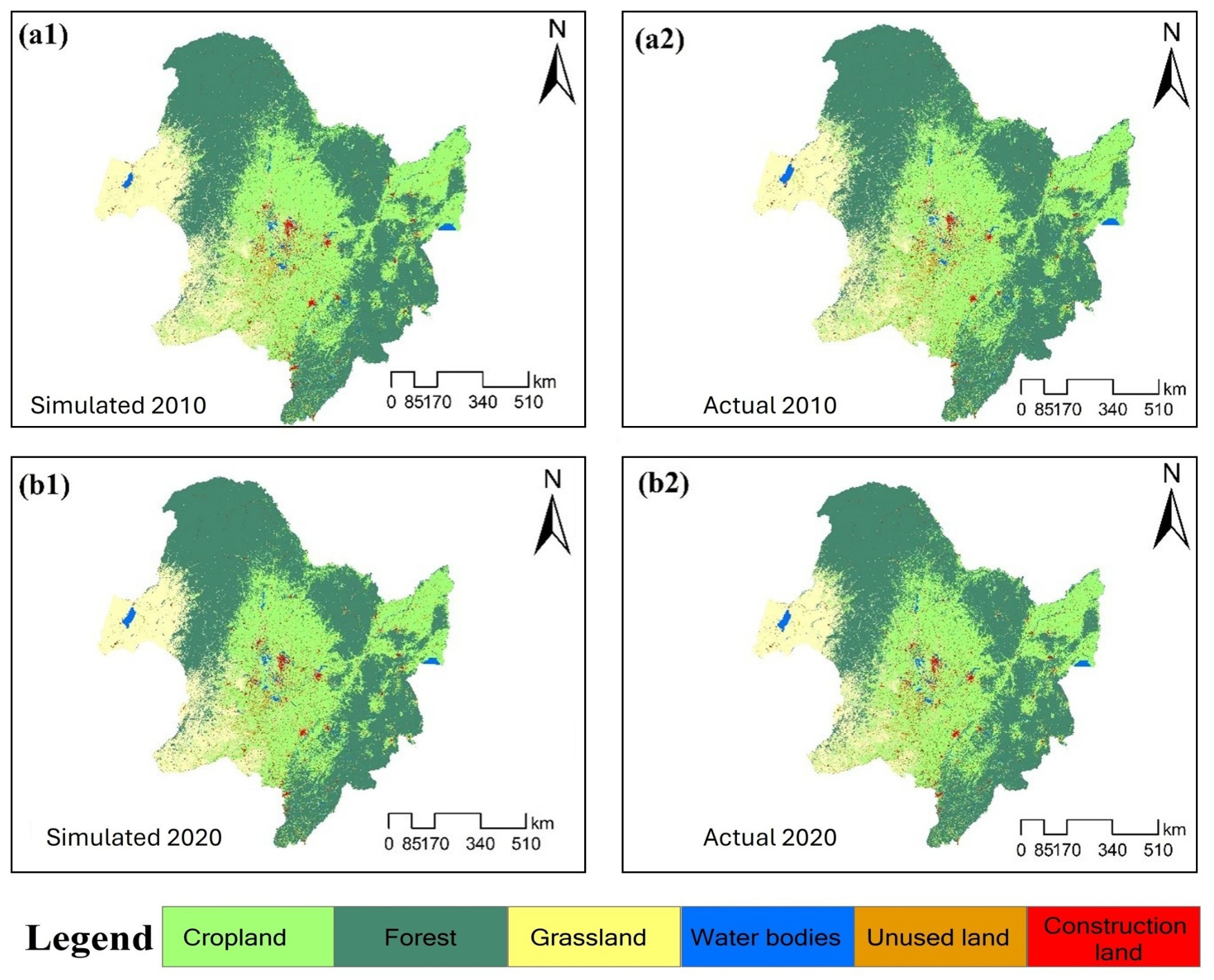
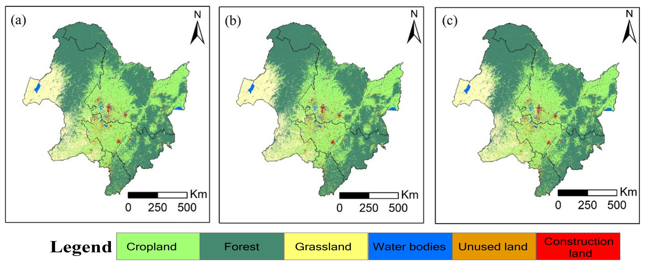
The FLUS validation results for the 2010 and 2020 simulations are shown in Figure 4. Quantitatively, the FLUS model showed acceptable validation performance across the historical validation periods. For the 2010 validation, OA, Kappa, and FoM were 0.914, 0.865, and 0.347, respectively. For the 2020 validation, OA, Kappa, and FoM were 0.880, 0.813, and 0.239, respectively. The corresponding confusion matrices and class-level producers’ and users’ accuracies for 2010 and 2020 are provided in Table S14. The simulated maps reproduced the major spatial patterns of observed LULC, particularly the dominance of Forest and Cropland and the concentration of Construction land in localized urban areas. By 2040, Forest and Cropland continued to dominate the landscape, together comprising approximately 82–83% of the total area across all SSP scenarios (

Table 2. Land-use area (km²) and area percentage (%) in 2020 and projected for 2040 under different SSP scenarios.

Land Type	2020 (km2)	2020 (%)	SSP1-2.6 (km2)	SSP1-2.6 (%)	SSP2-4.5 (km2)	SSP2-4.5 (%)	SSP5-8.5 (km2)	SSP5-8.5 (%)
Cropland	379,763	35.06	374,420	34.57	393,378	36.32	393,379	36.32
Forest	507,971	46.90	522,438	48.24	499,564	46.13	499,564	46.13
Grassland	146,888	13.56	137,947	12.74	133,580	12.33	133,614	12.34
Water bodies	13,608	1.26	13,607	1.26	13,496	1.25	13,461	1.24
Unused land	4612	0.43	3528	0.33	3183	0.29	3183	0.29
Construction land	30,199	2.79	31,101	2.87	39,840	3.68	39,840	3.68

Note: The reported 2040 class areas represent the realized FLUS allocation outputs under the fixed CA-Markov demand target and scenario-specific climate and socioeconomic suitability surfaces.

; Figure 5). However, the direction and magnitude of class-level changes varied among pathways. Under SSP1-2.6, Cropland decreased by 5343 km², whereas Forest increased by 14,467 km², indicating a more conservation-oriented land-allocation outcome. In contrast, Cropland expanded strongly under SSP2-4.5 and SSP5-8.5 by 13,615–13,616 km², while Forest declined by 8407 km² under both scenarios. Grassland contracted across all scenarios, with losses ranging from 8941 km² under SSP1-2.6 to 13,274–13,308 km² under SSP5-8.5 and SSP2-4.5. Construction land expanded in all scenarios, but the increase was much smaller under SSP1-2.6 (+902 km²) than under SSP2-4.5 and SSP5-8.5 (+9641 km²). Water bodies changed only slightly, while Unused land declined across all scenarios. Because a fixed 2040 land-demand target was used across SSP scenarios, differences among the projected LULC maps mainly reflect scenario-specific climate and socioeconomic suitability inputs rather than different policy- or management-driven demand assumptions. The close similarity between SSP2-4.5 and SSP5-8.5 is partly supported by their relatively similar 2040 climate inputs. Mean precipitation differed by only 5.94 mm yr⁻¹ between SSP2-4.5 and SSP5-8.5, compared with 17.81 mm yr⁻¹ between SSP1-2.6 and SSP2-4.5. Based on the average of Tmax and Tmin, mean temperature differed by approximately 0.16 °C between SSP2-4.5 and SSP5-8.5, compared with approximately 0.43 °C between SSP1-2.6 and SSP2-4.5 (Table S13). Therefore, under the fixed-demand FLUS design, SSP2-4.5 and SSP5-8.5 produced similar LULC allocation outputs, whereas the wetter and cooler SSP1-2.6 climate surface contributed to a more distinct allocation pattern. Overall, the 2040 LULC projections indicate persistent dominance of Forest and Cropland, Grassland contraction across all pathways, and stronger Cropland and Construction land expansion under the medium- and high-forcing pathways.

The controlled LULC perturbation assessment showed that future LULC allocation was generally stable, but instability varied clearly among land-cover classes. Class-level variation uncertainty indicated that allocation instability was concentrated mainly in small or transition-sensitive classes, whereas more spatially persistent classes showed lower instability. These results support the use of LULC allocation uncertainty as a supplementary diagnostic layer rather than as a replacement for the original FLUS scenario rasters. The scenario-specific class-level LULC allocation uncertainty results are provided in Figure S4.

3.2. Historical and Projected NDVI Dynamics

3.2.1. Historical Spatiotemporal Trends

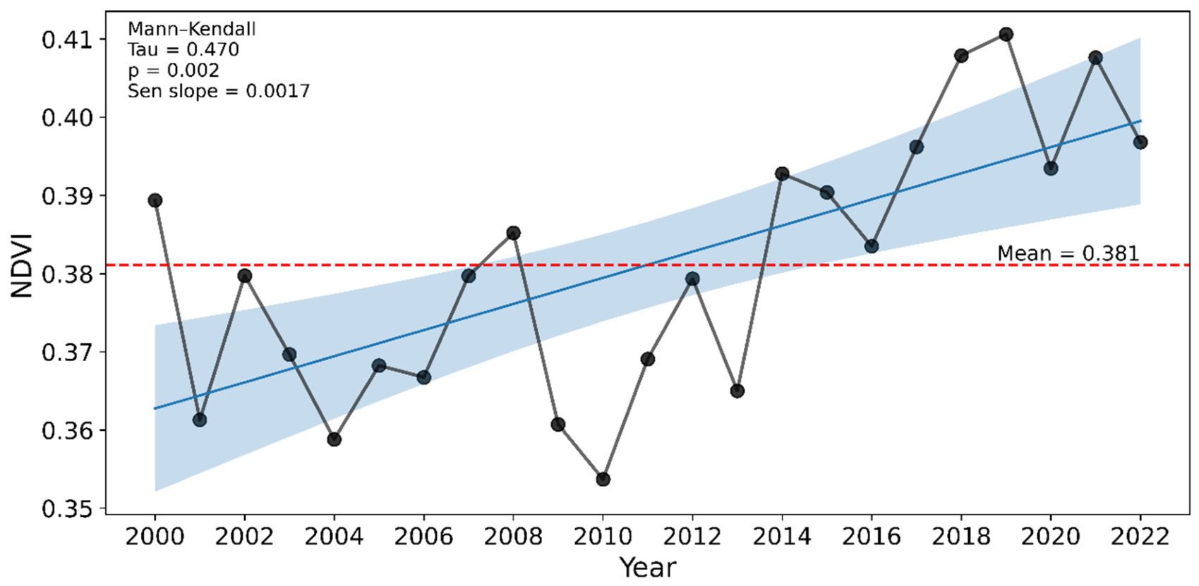
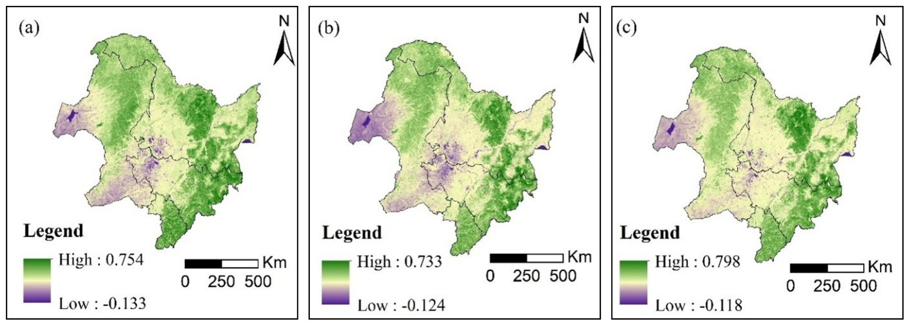
From 2000 to 2010, NDVI showed a decreasing trend, followed by recovery until 2022, with an overall increasing trend (Mann–Kendall Tau = 0.470, Sen’s slope = 0.0017, p = 0.002; Figure 6). Spatially, in 2000 and 2010, low NDVI was concentrated in the central and western interiors, while higher NDVI was sustained in eastern, northern, and elevated outer regions. By 2020, greening increased, characterized by enhanced high-NDVI coverage in surrounding regions, whereas low-NDVI cores remained consistently central (Figure 7). The historical trend analysis was extended to 2022 to provide a broader temporal context for regional greening dynamics, whereas model evaluation and holdout validation were anchored to 2020 to maintain a consistent independent test year.

3.2.2. Projected NDVI Under SSP Scenarios for 2040

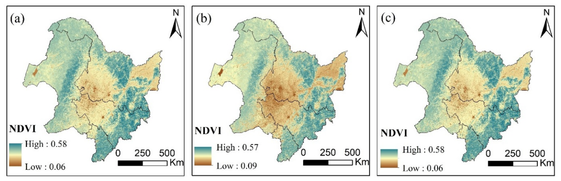
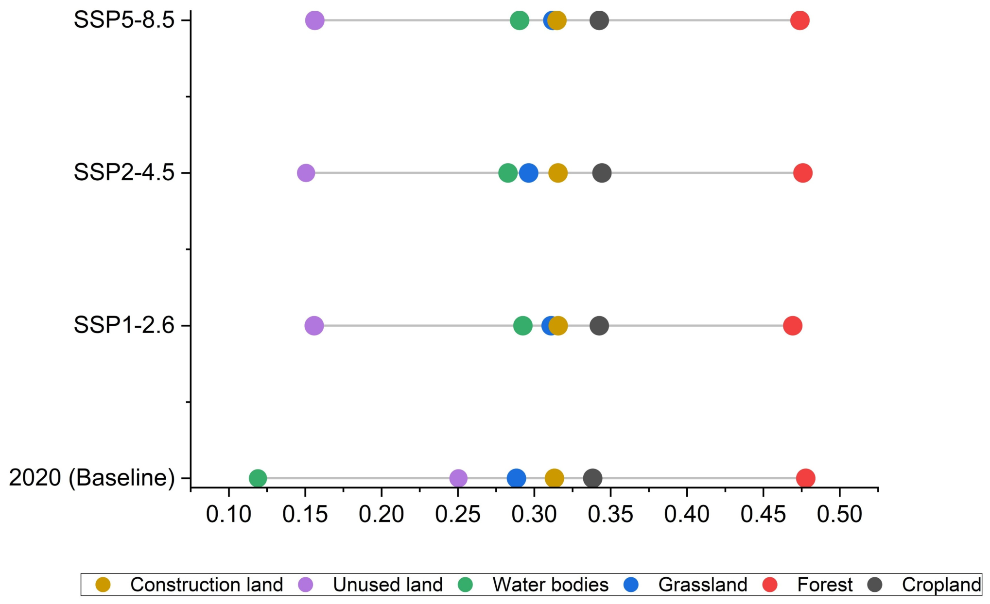
Projected NDVI maps for 2040 at 1 km resolution revealed marked spatial heterogeneity within each SSP scenario, while differences among scenarios remained limited (Figure 8). Regional mean NDVI varied only slightly across pathways, with the highest value under SSP5-8.5 (0.417), followed by SSP2-4.5 (0.415) and SSP1-2.6 (0.414). Despite this scenario convergence at the aggregate level, all three pathways indicated a consistent greening pattern relative to the 2020 baseline, reflected by contraction of low-NDVI interior zones and expansion of higher-NDVI peripheral areas (Figure 8 and Figure S6). These changes were strongly land-cover dependent (Figure 9): water bodies showed the largest increase (likely reflecting mixed-pixel contributions from riparian and shoreline vegetation at 1 km resolution rather than open-water greening; see Section 4.3), grassland increased moderately, cropland remained nearly stable, and Forest showed only a slight decline. In contrast, unused land decreased markedly, whereas construction land remained broadly stable with a slight increase.

3.3. Model Validation and Uncertainty

3.3.1. Candidate Model Comparison and Selection

Three candidate machine-learning models—Random Forest (RF), XGBoost (XGB), and LightGBM (LGBM)—were evaluated using five-fold spatial block cross-validation, primary temporal holdout validation, long-jump temporal extrapolation, and climatic perturbation tests. Under spatial block cross-validation, LGBM achieved the highest predictive performance, with R² = 0.654 ± 0.123 and RMSE = 0.056 ± 0.006, followed closely by XGB, whereas RF showed weaker spatial-transfer performance (Table S5). However, the spatial CV difference between LGBM and XGB was small, indicating that spatial block CV alone was not sufficient to justify final model selection.

In the primary temporal holdout validation experiment, where models were trained on 2000–2019 observations and evaluated against 2020 observations, LightGBM showed the strongest predictive performance, achieving the highest R² (0.710), the lowest RMSE (0.058), and the smallest absolute bias (−0.006). Although the relative ranking of RF and XGBoost differed from the spatial block cross-validation results, LightGBM remained the best-performing model under both evaluation settings (Table S5). The fold-level spatial block results further indicated differences in spatial transferability among models: RF showed poor generalization in one spatial partition (Fold 0, R² = −0.07), whereas LightGBM maintained positive performance across all five folds, with a minimum R² of 0.420 (Table S6). Together, these results support the selection of LightGBM for forward NDVI projection.

Under the more demanding long-jump extrapolation test, in which models were trained on 2000–2010 and tested against 2020, LGBM retained the strongest extrapolative performance, yielding the highest R² (0.671) and the lowest RMSE (0.062), whereas RF and XGB showed weaker long-horizon transferability (Table S7). In the climatic perturbation experiments, all models largely preserved spatial variability, as indicated by standard-deviation ratios close to one (Table S8). Among the candidate models, LGBM produced the standard-deviation ratio closest to one under the combined PRE + TEMP perturbation (0.998), indicating slightly better preservation of baseline spatial heterogeneity under future-like climatic forcing.

Taken together, these results indicate that LGBM provided the most balanced and consistent performance across spatial, temporal, extrapolative, and perturbation-based evaluation stages. Therefore, LGBM was selected as the final model for the 2040 NDVI projection. However, selecting the most suitable model for forward projection does not by itself establish uniform projection support across land-cover types; this requires holdout-based class-stratified evaluation of the 2020 prediction.

3.3.2. Stratified Validation per LULC Class

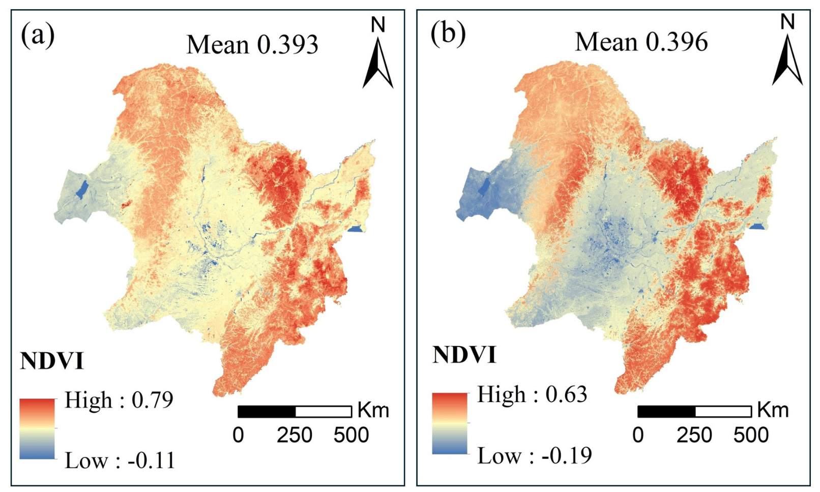
Class-stratified validation metrics for the selected LGBM model were computed using the independent 2020 prediction generated from the primary temporal validation framework (training in 2000–2019 and predicting 2020). Visual comparison between observed and predicted NDVI showed that the model broadly reproduced the main spatial pattern across NEC, although the predicted surface appeared smoother than the observed map and captured a narrower range of extreme values (Figure 10). The observed-versus-predicted scatter plot further revealed systematic overprediction at NDVI < 0.1 and underprediction above 0.55, with a fan-shaped heteroscedastic residual pattern concentrated in low-NDVI classes (Figure S5), consistent with the elevated errors for Water bodies and Unused land in

Table 3. Class-stratified validation and residual decomposition metrics for the independent 2020 NDVI prediction generated by training in 2000–2019 and testing in 2020.

LULC Class	n Pixels	R2	RMSE	MAE	Absolute Mean Residual	Residual STD
Cropland	379,763	0.388	0.046	0.032	0.003	0.046
Forest	507,971	0.528	0.061	0.047	0.002	0.061
Grassland	146,888	0.540	0.049	0.036	0.012	0.047
Water bodies	13,608	−0.586	0.209	0.172	0.156	0.138
Unused land	4612	−0.886	0.116	0.096	0.079	0.085
Construction land	30,199	0.576	0.060	0.043	0.001	0.060

. Mean NDVI was similar between the observed and predicted maps (0.393 and 0.396, respectively). However, predictive performance varied markedly among land-cover classes (Table 3). Among the classes with positive explanatory performance, Construction land showed the highest R² (0.576), followed by Grassland (0.540) and Forest (0.528), whereas Cropland showed more moderate performance (R² = 0.388). In contrast, Water bodies and Unused land performed poorly, with negative R² values (−0.586 and −0.886, respectively). Water bodies showed the largest absolute errors (RMSE = 0.209; MAE = 0.172). Overall, the apparent agreement between observed and predicted regional NDVI patterns masked substantial class-dependent differences in predictive skill.

Residual zonal statistics further clarified the structure of model error across LULC classes (Table 3). Construction land showed the smallest absolute mean residual (0.001), followed by Forest (0.002) and Cropland (0.003), indicating limited systematic deviation in these classes. Grassland showed a moderate absolute mean residual (0.012) relative to a comparatively low residual standard deviation (0.047). Water bodies exhibited both the largest absolute mean residual (0.156) and the highest residual standard deviation (0.138), whereas Unused land showed the second-highest absolute mean residual (0.079) and a relatively high residual standard deviation (0.085). These results indicate that both the magnitude and composition of model error varied across land-cover classes.

3.3.3. Projection Uncertainty and URI Analysis

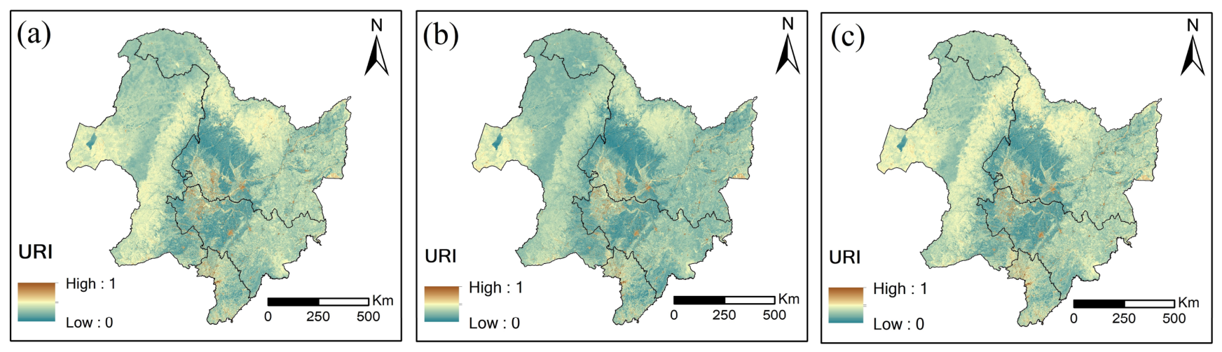
To complement the historical error structure revealed by class-stratified validation, relative projection uncertainty was then characterized to compare how uncertainty patterns varied spatially and across land-cover classes under the three SSP scenarios. After model selection and independent class-wise validation, projection uncertainty for 2040 was quantified using the URI derived from the 95% prediction interval estimated by LightGBM quantile regression models. Accordingly, URI values should be interpreted comparatively across space, classes, and scenarios within the current framework, rather than as absolute measures of probabilistic prediction failure. Spatially, high URI values were concentrated in central-interior zones and construction land-dominated areas, whereas cropland- and Forest-dominated regions showed persistently lower uncertainty across all SSP scenarios (Figure 11). The overall URI pattern remained broadly consistent among scenarios, indicating scenario-robust spatial uncertainty structure. At the class level, Construction land consistently showed the highest mean URI across SSP1-2.6, SSP2-4.5, and SSP5-8.5 (0.553, 0.563, and 0.554, respectively), whereas Cropland showed the lowest uncertainty (0.198, 0.193, and 0.204). Unused land ranked second in mean uncertainty across all scenarios, while Water bodies and Grassland occupied intermediate positions (

Table 4. URI zonal statistics per LULC class across SSP scenarios.

LULC Class	SSP1-2.6 Mean	SSP2-4.5 Mean	SSP5-8.5 Mean
Cropland	0.198	0.193	0.204
Forest	0.252	0.225	0.265
Grassland	0.278	0.261	0.284
Water bodies	0.303	0.284	0.299
Unused land	0.386	0.375	0.384
Construction land	0.553	0.563	0.554

). Across all classes, SSP2-4.5 tended to produce the lowest or near-lowest mean URI, suggesting that the intermediate emission pathway generates climate and socioeconomic forcing closest to the centroid of the historical training distribution, thereby reducing quantile-interval width; however, scenario differences within each class were small relative to between-class differences and do not alter the overall class-level uncertainty ranking.

3.4. Driver Analysis and Validation Priority

3.4.1. SHAP-Based Driver Contributions to NDVI Dynamics

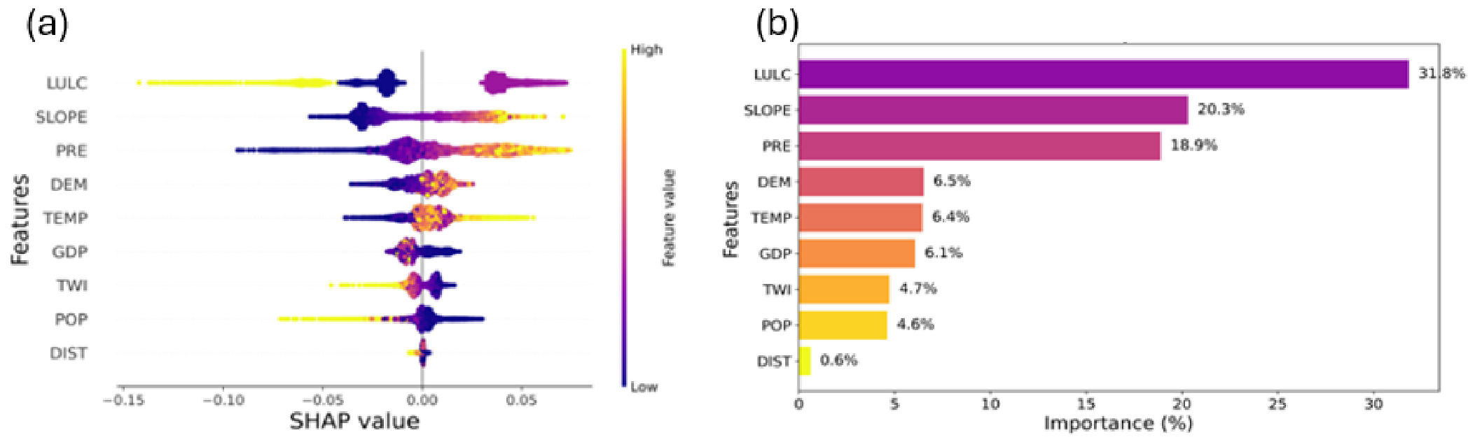
SHAP-based feature importance analysis showed that Land Use/Land Cover (LULC) was the most influential predictor of NDVI spatial variability across NEC, accounting for 31.8% of total feature importance, approximately 1.5 times greater than any other variable (Figure 12b). Directional analysis further revealed distinct class-dependent SHAP effects for LULC, suggesting strong differences in NDVI response among land-cover classes (Figure 12a). Slope and precipitation ranked as the second and third most influential predictors (20.3% and 18.9%, respectively), with higher values of both variables generally associated with positive SHAP contributions to NDVI (Figure 12a,b). DEM, TEMP, and GDP exhibited intermediate and broadly comparable contributions (6.5%, 6.4%, and 6.1%, respectively), whereas TWI and POP remained relatively minor predictors. Population density displayed a predominantly negative SHAP pattern (Figure 12a), whereas DIST had the weakest contribution, accounting for only 0.6% of total feature importance (Figure 12b). Temporal comparison across 2000, 2010, and 2020 further revealed a modest decline in the relative importance of precipitation and a corresponding increase in the contribution of slope, suggesting an increasing relative importance of topographic control over time (Figure 12 and Figure S7). Because LULC was the dominant predictor, class-level differences in vegetation–environment relationships constitute the primary structural source of prediction variability across NEC, directly motivating the land-cover-stratified validation approach applied in Section 3.3.2 rather than globally aggregated accuracy metrics alone.

3.4.2. Priority Ranking for Future Validation

Integrating systematic error, random error, and future URI into a combined priority score showed that Water bodies had the highest validation priority (0.784), followed by Unused land (0.667), Construction land (0.477), and Grassland (0.220). Forest and Cropland showed the lowest priority scores (0.153 and 0.000, respectively), reflecting their relatively low residual errors and low to moderate future uncertainty (

Table 5. Combined priority score for future validation per LULC class.

Rank	LULC Class	Sys. Error	Rand. Error	Mean URI	Priority Score	Main Validation Issue
1	Water bodies	0.824	1.000	0.271	0.784	High random and systematic error
2	Unused land	1.000	0.413	0.512	0.667	Systematic bias with moderate URI
3	Construction land	0.471	0.222	1.000	0.477	Highest future uncertainty
4	Grassland	0.412	0.032	0.212	0.220	Moderate systematic bias
5	Forest	0.059	0.254	0.137	0.153	Low concern; minor scatter
6	Cropland	0.000	0.000	0.000	0.000	Lowest validation priority

Note: Sys. Error = min–max normalized absolute mean residual from Table 3; RAND. Error = min–max normalized residual STD from Table 3; Mean URI = min–max normalized mean URI across SSP1-2.6, SSP2-4.5, and SSP5-8.5 (Table 4). Priority Score = 0.4 × Norm. Systematic + 0.4 × Norm. Random + 0.2 × Norm. URI Mean. All components were independently rescaled to [0, 1] prior to weighted aggregation. Cropland receives a priority score of 0.000 because min–max normalization anchors the minimum-value class to zero on all three components simultaneously. Its absolute metric values are reported in Table 3.

). Cropland’s score of exactly 0.000 results from min–max normalization, simultaneously anchoring the class with the lowest value on all three components to zero; its absolute error metrics remain non-zero (Table 3). A critical finding is that the sources of validation priority differ markedly among land-cover classes. Water bodies rank first because they combine high systematic error (Norm. Systematic Error = 0.824) with the highest random error (Norm. Random Error = 1.000), indicating a compounded form of validation priority that is unlikely to be resolved by a single global model adjustment. Unused land ranks second primarily because it has the highest normalized systematic error (1.000), despite only moderate future URI (Norm. URI Mean = 0.512). Construction land ranked third because it has the highest normalized URI mean (1.000), indicating future-driven rather than historically driven risk. Grassland ranks fourth because its priority is driven mainly by moderate systematic error rather than random instability or future uncertainty, suggesting that targeted bias correction may substantially improve class-level performance. Sensitivity analysis across four alternative weighting schemes showed that the priority extremes and overall rank ordering remained stable, with Water bodies, Unused land, Construction land, and Cropland consistently ranked first, second, third, and last, respectively (

Table 6. Sensitivity analysis of the three-component priority score and supplementary LAII-informed robustness test.

LULC Class	Original	Equal	URI-Heavy	History-Heavy	LAII Score	Orig. Rank	LAII Rank	Change
Water bodies	0.784	0.691	0.656	0.839	0.754	1	1	0
Unused land	0.667	0.635	0.629	0.716	0.529	2	2	0
Construction land	0.477	0.559	0.608	0.424	0.260	3	3	0
Grassland	0.220	0.216	0.218	0.240	0.117	4	4	0
Forest	0.153	0.149	0.149	0.145	0.072	5	5	0
Cropland	0.000	0.000	0.000	0.000	0.035	6	6	0

Note: Original, Equal, URI-heavy, and History-heavy scores test the sensitivity of the original three-component priority score to alternative weights assigned to systematic error, random error, and URI mean. The LAII-informed score is a separate, supplementary robustness test that adds the normalized LULC Allocation Instability Index (LAII) as a fourth component using weights 0.35/0.35/0.20/0.10 for systematic error, random error, URI mean, and LAII, respectively. Rank change is calculated relative to the original three-component score.

).

To further test whether the validation-priority ranking was sensitive to future LULC allocation instability, LAII was added as a fourth normalized component in a supplementary robustness score. Incorporating LAII did not alter the class-level priority ranking: Water bodies, Unused land, and Construction land remained the three highest-priority classes, whereas Cropland remained the lowest-priority class. This confirms that the validation-priority structure was robust not only to alternative weighting assumptions, but also to LULC allocation instability. The result also indicates that LAII added complementary information without overturning the main interpretation of class-level validation priority.

4. Discussion

4.1. Projection-Oriented Model Selection for Future NDVI Assessment

Model comparison across evaluation stages supported the selection of LightGBM as the most suitable model for forward NDVI projection under the assessment framework adopted here. Rather than relying on a single validation metric, the study evaluated candidate models using spatial block cross-validation, short-gap temporal transfer, longer-horizon temporal extrapolation, and controlled climatic perturbation. Under this design, model selection was treated as an extrapolation-oriented assessment step intended to identify the model with the most balanced performance profile for forward projection, rather than the model that performed best under one validation setting alone.

This multi-stage model-selection strategy is consistent with previous recommendations for spatial and temporal prediction problems, where random or single-scheme validation can overestimate model transferability when data are spatially or temporally structured. Roberts et al. [37] emphasized that cross-validation should reflect the intended prediction task when ecological data contain spatial or temporal structure, while Meyer and Pebesma [38] showed that spatial predictions become less reliable when target conditions fall outside the predictor space represented by the training data. This supports the use of temporal holdout and long-jump extrapolation as central criteria for evaluating model suitability for 2040 NDVI projection, rather than relying on spatial cross-validation alone.

Across these tests, LightGBM showed the most consistent overall performance. It achieved the highest accuracy under spatial block cross-validation (R² = 0.654 ± 0.123; RMSE = 0.056 ± 0.006), outperformed both XGBoost and Random Forest in the primary temporal validation for 2020 (R² = 0.710; RMSE = 0.058; bias = −0.006), and retained the best performance under the more demanding long-jump extrapolation from 2000 to 2010 to 2020 (R² = 0.671; RMSE = 0.062). Notably, XGBoost showed near-identical spatial CV performance to LightGBM (R² = 0.646 vs. 0.654), but a substantially larger drop in temporal holdout performance (R² = 0.511 vs. 0.710). This divergence would have been obscured under spatial CV alone and reinforces the value of multi-stage evaluation over single-metric model selection. Although the primary temporal holdout was limited to the terminal historical year 2020, this design was supplemented by spatial block cross-validation, a longer-horizon 2000–2010 to 2020 extrapolation test, and climatic perturbation experiments to reduce dependence on a single validation criterion. Additionally, fold-level inspection (Table S6) showed that Fold 3 produced the lowest R² across all three models, suggesting it captures the central-interior low-NDVI subregion where Water bodies and Unused land are concentrated—the same classes that showed the weakest performance in class-stratified validation (Table 3). Taken together, these results indicate that LightGBM provided the most consistent performance profile for forward NDVI projection under the multi-stage assessment design used here.

The climatic perturbation experiments provided an additional diagnostic perspective on model robustness under future-like conditions. All three models largely preserved spatial variability, but LightGBM yielded the combined-perturbation standard-deviation ratio closest to 1 (0.998), indicating slightly better preservation of baseline spatial heterogeneity. The perturbation test served primarily as a diagnostic robustness check rather than as a strong basis for differential model selection, given that all three models produced standard-deviation ratios within ±0.01 of baseline under the applied perturbation magnitudes. The selection of LightGBM therefore rests primarily on its consistent advantage across temporal holdout and long-jump extrapolation, supported by the highest, although marginal, spatial CV performance. The SHAP results further support this modeling framework by identifying LULC, slope, and precipitation as the dominant controls on modeled NDVI variability, suggesting that the selected model captured a predictor structure that was both stable and ecologically interpretable.

The tree-based framework was selected to support interpretable predictor-contribution analysis using SHAP and controlled perturbation diagnostics, while avoiding the additional computational and interpretability complexity often associated with equivalent analyses in deep-learning architectures. Future work may evaluate whether recurrent, convolutional, or attention-based models produce different class-level error structures within the same stratified validation framework.

4.2. Land Cover-Specific Validation and Error Decomposition

Class-stratified validation revealed that the LightGBM model’s overall temporal holdout performance concealed substantial variation in class-level predictive support. Although the model achieved an overall temporal holdout R² of 0.710, class-level R² values ranged from 0.576 to −0.886, confirming that global accuracy metrics are insufficient to characterize projection reliability in heterogeneous landscapes. Construction land, Grassland, and Forest showed positive explanatory performance, with R² values of 0.576, 0.540, and 0.528, respectively, while Cropland showed more moderate performance (R² = 0.388). In contrast, Water bodies and Unused land showed negative R² values (−0.586 and −0.886), indicating that the model explained less variance than a simple class-mean predictor for these two classes.

Among the better-performing classes, the relatively stable performance of Forest and Cropland is likely associated with their large sample sizes, broad spatial representation, and more consistent vegetation–environment relationships within the training data. Construction land performed best despite its smaller sample size, possibly because construction land-dominated pixels in NEC have a more distinctive predictor signature and a relatively consistent mixed impervious–vegetated composition. Grassland showed a moderate absolute mean residual (0.012) relative to a low residual standard deviation (0.047), indicating that its error structure was more strongly associated with directional bias than random scatter. This suggests that targeted bias correction may improve class-level performance for Grassland more effectively than major restructuring of the global model.

The negative R² values for Water bodies and Unused land reflect a combination of structural and class-specific limitations. Structurally, both classes were severely underrepresented in the training data—Water bodies (13,608 pixels) and Unused land (4612 pixels) together constituted less than 2% of training samples relative to the Forest- and Cropland-dominated pixel pool, giving the global model limited incentive to learn their class-specific signal structure. At the class level, poor performance for Water bodies likely reflects sub-pixel mixing at 1 km resolution, where MODIS-derived NDVI integrates signals from open water, shoreline vegetation, aquatic macrophytes, exposed sediment, and riparian wetland margins, weakening the interpretation of NDVI as a stable vegetation signal [39,40,41]. This explains both its high systematic deviation, represented by an absolute mean residual of 0.156, and its high random error, represented by a residual STD of 0.138. For Unused land, weak performance likely reflects high within-class heterogeneity, as this category includes bare soil, sparse scrub, degraded grassland margins, and saline surfaces with contrasting NDVI responses [42]. Sparse vegetation and exposed soil also increase the influence of soil background on red and near-infrared reflectance, which is a fundamental limitation of NDVI-type indices in low-cover environments [43]. Construction land should also be interpreted cautiously despite its positive class-level performance because urban pixels commonly contain mixtures of vegetation, impervious surfaces, and bare soil, consistent with impervious-surface-based urban remote-sensing studies [44]. Therefore, model refinement should address both training imbalance and class-specific spectral complexity through weighted loss functions, stratified resampling, class-specific covariates, or dedicated sub-models for poorly represented and spectrally heterogeneous classes.

4.3. Future NDVI Trajectories Under Scenario Constraints

Projected NDVI for 2040 showed a consistent greening pattern across all SSP scenarios relative to the 2020 baseline, with regional mean NDVI increasing from 0.393 to 0.414–0.417. To assess consistency with the observed historical trajectory, these projected values were compared with a simple linear extrapolation of the Mann–Kendall trend. Applying the Sen’s slope of 0.0017 yr⁻¹ over 2020–2040 to the 2020 baseline gives an extrapolated estimate of approximately 0.427, around 0.010–0.013 NDVI units above the model-projected range. Because this difference falls within the temporal validation RMSE of the selected LightGBM model, it should be interpreted as a directional signal rather than a large absolute discrepancy. Nevertheless, the systematic departure from linear extrapolation suggests that the scenario-driven model does not simply continue the historical greening trend but indicates a moderated greening response by 2040. This moderation is ecologically plausible because warming benefits may weaken as growing-season temperatures approach or exceed ecological optima, and because already-greened Forest and cropland pixels may have limited capacity to continue increasing at the historical rate [45,46].

The limited scenario divergence at the regional level, with only 0.003 NDVI units separating the three SSP pathways by 2040, should therefore be interpreted as a near-term, time-horizon-dependent result rather than evidence that SSP forcing is unimportant.

However, limited divergence in regional mean NDVI does not imply that SSP scenarios produced similar land-cover trajectories. At the class level, construction land expansion differed by about eleven-fold between SSP1-2.6 and SSP2-4.5/SSP5-8.5 (+902 versus +9641 km²), while Forest showed opposite trajectories, increasing under SSP1-2.6 (+14,467 km²) but decreasing under SSP2-4.5/SSP5-8.5 (−8407 km²).

These contrasting class-level dynamics can partly offset one another in regional averages, providing a key reason why class-stratified assessment is more informative than aggregate reporting alone. This pattern is directionally consistent with independent CMIP6-based vegetation projections for NEC. Yuan et al. [47] projected continued increases in growing-season mean LAI in Northeast China, with larger increases under SSP5-8.5 than SSP2-4.5: 0.40 versus 0.27 during 2041–2070, and 0.70 versus 0.39 during 2071–2100. Thus, the difference between SSP5-8.5 and SSP2-4.5 increases from approximately 0.13 LAI units at mid-century to 0.31 LAI units by late-century, indicating that scenario divergence becomes stronger after mid-century. Although LAI and NDVI are not interchangeable and should not be converted directly, this directional pattern supports the interpretation that weak SSP separation by 2040 is expected at a near-term horizon. Nguyen et al. [14] similarly reported that global mean NDVI under SSP5-8.5 can be higher than under lower-emission pathways during 2021–2040 before high-emission impacts become more negative later in the century. Therefore, the slightly higher NDVI under SSP5-8.5 in this study should be interpreted as a near-term response in a temperature-limited region, not as evidence of long-term ecological benefit under high-emission forcing. Beyond 2040, stronger warming, increasing drought risk, and permafrost-related ecological changes may progressively weaken or reverse this warming-driven greening signal in Northern NEC [47,48].

At the class level, projected NDVI trajectories should not be conflated with changes in land-cover area, because each reflects a different process. Water bodies showed increasing mean NDVI despite slight area contraction, most likely because 1 km water pixels include mixed vegetated surfaces such as shoreline vegetation, aquatic macrophytes, and riparian wetland margins rather than open water alone [40,41]. Unused land showed declining mean NDVI through a different mechanism: as the most actively converted class in the projected LULC maps, the pixels remaining as unused land by 2040 likely represent comparatively less vegetated or more environmentally constrained surfaces. Construction land showed a slight mean NDVI increase, but this should also be interpreted cautiously because 1 km construction land pixels may contain parks, street trees, peri-urban agricultural patches, and vegetated industrial margins rather than uniformly impervious surfaces [44]. Moreover, Construction land consistently exhibited the highest URI across SSP scenarios, indicating disproportionately high future projection uncertainty despite its moderate historical residual profile. These class-specific patterns confirm that regional mean NDVI alone is insufficient to characterize projection support: modest greening and weak SSP separation at the aggregate level conceal distinct class-level mechanisms, uncertainty sources, and validation needs. Ecologically, the modest NDVI increase projected for NEC by 2040 suggests a continuation of regional greening in a landscape dominated by cropland and forest. In forested areas, this greening may indicate stronger canopy activity and potential carbon-sink support, whereas in cropland it may reflect maintained vegetation productivity and possible crop-yield support [1,2]. However, because NDVI represents vegetation greenness rather than ecosystem function directly, its implications for biodiversity and ecosystem-service provision may differ among land-cover types [1,49]. Greening in intensively managed cropland or construction land margins may not necessarily represent habitat improvement, while the higher validation priority identified for Water bodies, Unused land, and Construction land indicates where NDVI-based ecological interpretation should be supported by complementary indicators such as carbon storage, crop yield, habitat quality, and land-use intensity.

4.4. Linking Historical Prediction Errors to Future Validation Priorities

Integrating historical validation residuals with projected URI values across SSP scenarios revealed that class-level validation priority was not determined by historical model accuracy alone. Historical residuals describe how the model performed under observed conditions, whereas URI provides a forward-looking indication of relative uncertainty under future scenario inputs. Therefore, classes with similar historical accuracy may still differ in future validation priority if their projected uncertainty differs substantially.

Water bodies showed the highest priority score (0.784), mainly because they combined high normalized systematic error (0.824) with the highest normalized random error (1.000), despite only moderate normalized future URI (0.271). This indicates that the weak projection support for Water bodies is primarily rooted in historical model-performance limitations, including both directional bias and spatial variability. In contrast, Unused land ranked second (0.667) because of the highest normalized systematic error (1.000), together with moderate random error (0.413) and moderate future URI (0.512), indicating that systematic deviation is the dominant issue in this class. Construction land ranked third (0.477), not because of especially large historical residuals, but because it showed the highest normalized future URI (1.000), suggesting that future relative uncertainty associated with construction land-dominated and urban-expansion areas may become more important than its historical error profile alone would indicate. Grassland ranked fourth (0.220), with moderate normalized systematic error (0.412) but very low normalized random error (0.032), implying that its prediction limitations may be more responsive to bias correction than to major structural redesign of the model.

The LAII-informed robustness analysis further strengthened the historical–future linkage by adding a diagnostic layer for future LULC allocation instability. Because LULC was the dominant predictor of modeled NDVI variability, instability in future land-cover allocation represents an additional source of projection concern. LAII was not intended to fully propagate land-cover uncertainty through the NDVI model, but to test whether validation priorities were sensitive to this input uncertainty. The unchanged ranking after adding LAII indicates that the main priorities were not driven solely by the original three-component score. Water bodies remained a high priority mainly because of historical NDVI prediction errors, whereas Unused land and Construction land were additionally supported by future uncertainty and LULC allocation sensitivity.

This result is consistent with the remote-sensing accuracy-assessment literature, which has long emphasized that overall or aggregate metrics can conceal substantial class-level errors. Land-cover assessment should not rely only on global accuracy summaries because different classes may have different error structures [50], and class-specific accuracy and uncertainty reporting are recommended to support transparent interpretation of land-change products [51]. In this context, the combined priority score used here extends the same principle from land-cover map assessment to NDVI projection reliability: classes with limited area or complex spectral composition may contribute little to aggregate model error but still require targeted validation because of their ecological or management importance.

Taken together, these results show that R² alone is insufficient for identifying validation priorities. Historical residual structure, future projection uncertainty, and LULC allocation instability provide complementary evidence for determining where projected NDVI patterns are better supported and where additional validation effort is most needed. In Northeast China, the 2040 NDVI projections showed only modest divergence among SSP pathways, but support for those projected patterns varied markedly across land-cover classes.

4.5. Limitations and Future Perspectives

This study has several limitations that should be acknowledged. First, the projection framework relies on remote-sensing-derived NDVI and a data-driven tree-based model without independent ground-based ecological validation; therefore, the reported performance reflects agreement with satellite-derived NDVI rather than direct ecological accuracy. LightGBM does not impose explicit plant physiological or ecohydrological constraints on vegetation responses, so projections under future conditions should be interpreted as statistically learned responses based on historical predictor–NDVI relationships and near-term perturbation ranges, rather than as process-based simulations of vegetation physiology. Similarly, GDP and population density were included as SSP-consistency socioeconomic covariates rather than direct causal ecological drivers, and their modeled effects should be interpreted as associative signals of human activity and land-use context. Future work should compare this framework with process-based or hybrid models incorporating physiological constraints on vegetation productivity, water stress, and temperature response.

Second, the climate and land-cover inputs carry their own uncertainties. Although the WorldClim v2.1 CMIP6 products used in this study are downscaled and bias-corrected, and although the inter-GCM spread was summarized in Table S13, the historical skill of the individual raw GCMs over NEC was not independently evaluated. In addition, the pixel-wise multi-model ensemble mean may smooth GCM-specific or localized climate extremes, potentially underestimating degradation risk under future heat, drought, or precipitation anomalies. Future land-use patterns from the FLUS model were treated as deterministic inputs in the main NDVI projections; the supplementary LAII-informed analysis evaluated allocation instability but did not constitute full propagation of LULC uncertainty into NDVI prediction. Future studies should screen individual GCMs against historical NEC observations and propagate multiple LULC realizations directly through the NDVI model.

Third, the Uncertainty Risk Index is a relative indicator derived from prediction-interval width under study-area-wide normalization, which preserves between-class differences but may underrepresent within-class uncertainty patterns. Future work could compare global and class-specific URI formulations to evaluate the sensitivity of the priority ranking to normalization choice.

Fourth, the framework relies on MODIS-derived NDVI harmonized to a 1 km modeling grid and on a single primary machine-learning model. MODIS NDVI may saturate in dense forest canopies, reducing sensitivity to high-biomass vegetation changes. Future studies should incorporate solar-induced chlorophyll fluorescence (SIF) or gross primary productivity (GPP) as complementary indicators and should apply higher-resolution or multi-model frameworks to reduce mixed-pixel effects in heterogeneous classes such as Water bodies and Construction land.

5. Conclusions

This study demonstrated that land-cover-stratified validation and uncertainty-informed priority ranking reveal class-specific projection limitations that aggregate accuracy metrics conceal—applied here at 1 km resolution across Northeast China (NEC) for 2040 under SSP1-2.6, SSP2-4.5, and SSP5-8.5.

(1)

All SSP scenarios indicate enhanced regional greening by 2040, with mean NDVI increasing from 0.393 in 2020 to 0.414–0.417. Although this overall greening signal is consistent across scenarios, projected responses are not spatially uniform and vary substantially among land-cover classes: Water bodies show the largest increase, Grassland shows a moderate increase, Cropland remains nearly stable, Forest shows a slight decline, Unused land decreases markedly, and Construction land remains broadly stable with a slight increase.

(2)

Model performance varied across evaluation stages, but LightGBM showed the most consistent overall performance. It achieved the highest accuracy under internal spatial block cross-validation and short-gap temporal validation, retained the strongest long-horizon extrapolation performance, and showed near-preservation of baseline spatial variability under the combined climatic perturbation. Taken together, LightGBM showed the most balanced and consistent performance across the evaluation stages and was therefore selected for the 2040 projection.

(3)

Independent class-stratified validation based on the 2020 holdout prediction revealed substantial land-cover-specific performance heterogeneity. Among the classes with positive explanatory performance, Construction land showed the highest R² (0.576), followed by Grassland (0.540) and Forest (0.528), whereas Cropland showed more moderate performance (R² = 0.388). In contrast, Water bodies and Unused land performed poorly, with negative R² values (−0.586 and −0.886, respectively). Water bodies exhibited the largest absolute errors (RMSE = 0.209), confirming that global model skill can mask major class-level differences in predictive performance.

(4)

Decomposition of residual error into systematic and random components showed that prediction limitations differ fundamentally among land-cover classes. Construction land, Forest, and Cropland showed limited systematic deviation, whereas Grassland showed a moderate systematic component relative to comparatively low random scatter. By contrast, Water bodies combined the strongest systematic deviation with the highest random variability, and Unused land also showed substantial residual error. These differences indicate that class-specific model refinement and future validation should be prioritized differently across land-cover types.

(5)

SHAP analysis showed that LULC was the dominant predictor of NDVI throughout the study period, while precipitation and slope were the next most influential drivers, with stable directional relationships across years. This supports the ecological interpretability of the LightGBM model and the inclusion of scenario-specific LULC as a central input to future NDVI projection.

(6)

Integrating historical residuals with future URI across SSP scenarios identified Water bodies, Unused land, and Construction land as the highest-priority classes for future targeted validation, reflecting different combinations of systematic deviation, random error, and projected future uncertainty. The priority ranking of Water bodies, Unused land, and Construction land should not be interpreted as a purely statistical outcome. These classes combine limited spatial representation with intrinsic NDVI modeling challenges, including weak vegetation signal, mixed pixels, and heterogeneous surface composition. Targeted field validation and class-specific model refinement are therefore particularly important for these classes.

Overall, this study shows that future NDVI projection assessment in heterogeneous landscapes should move beyond spatial prediction maps and global accuracy metrics. The proposed framework provides a diagnostic basis for evaluating class-specific projection support by integrating extrapolation-oriented model selection, land-cover-stratified validation, residual decomposition, relative uncertainty characterization, and validation-priority ranking. It can support targeted field validation, class-specific model refinement, and more transparent interpretation of future vegetation projections under climate and land-use change. With appropriate local calibration and validation, the framework can be extended to other heterogeneous regions.

References

1. Pettorelli, N.; Vik, J.O.; Mysterud, A.; Gaillard, J.-M.; Tucker, C.J.; Stenseth, N.C. Using the satellite-derived NDVI to assess ecological responses to environmental change. Trends Ecol. Evol. 2005, 20, 503–510. [Google Scholar] [CrossRef] [PubMed]
2. Xue, L.; Kappas, M.; Wyss, D.; Wang, C.; Putzenlechner, B.; Thi, N.P.; Chen, J. Assessment of climate change and human activities on vegetation development in Northeast China. Sensors 2022, 22, 2509. [Google Scholar] [CrossRef] [PubMed]
3. Jiang, L.; Liu, Y.; Wu, S.; Yang, C. Analyzing ecological environment change and associated driving factors in China based on NDVI time series data. Ecol. Indic. 2021, 129, 107933. [Google Scholar] [CrossRef]
4. Ma, M.; Wang, Q.; Liu, R.; Zhao, Y.; Zhang, D. Effects of climate change and human activities on vegetation coverage change in northern China considering extreme climate and time-lag and -accumulation effects. Sci. Total Environ. 2023, 860, 160527. [Google Scholar] [CrossRef] [PubMed]
5. Wu, R.; Wang, Y.; Liu, B.; Li, X. Spatial-temporal changes of NDVI in the three northeast provinces and its dual response to climate change and human activities. Front. Environ. Sci. 2022, 10, 974988. [Google Scholar] [CrossRef]
6. Wang, Y.; Zhang, N.; Chen, M.; Zhao, Y.; Guo, F.; Huang, J.; Peng, D.; Wang, X. Prediction and spatiotemporal dynamics of vegetation index based on deep learning and environmental factors in the Yangtze River Basin. Forests 2025, 16, 460. [Google Scholar] [CrossRef]
7. Meng, Z.; Lu, Y.; Wang, H. Correlation change analysis and NDVI prediction in the Yellow River Basin of China using complex networks and GRNN-PSRLSTM. Environ. Monit. Assess. 2024, 196, 1092. [Google Scholar] [CrossRef] [PubMed]
8. Guo, Y.; Zhang, L.; He, Y.; Cao, S.; Li, H.; Ran, L.; Ding, Y.; Filonchyk, M. LSTM time series NDVI prediction method incorporating climate elements: A case study of Yellow River Basin, China. J. Hydrol. 2024, 629, 130518. [Google Scholar] [CrossRef]
9. Ahmad, R.; Yang, B.; Ettlin, G.; Berger, A.; Rodríguez-Bocca, P. A machine-learning based ConvLSTM architecture for NDVI forecasting. Int. Trans. Oper. Res. 2023, 30, 2025–2048. [Google Scholar] [CrossRef]
10. Khodadadi, N.; Towfek, S.K.; Zaki, A.M.; Alharbi, A.H.; Khodadadi, E.; Khafaga, D.S.; Abualigah, L.; Ibrahim, A.; Abdelhamid, A.A.; Eid, M.M. Predicting normalized difference vegetation index using a deep attention network with bidirectional GRU: A hybrid parametric optimization approach. Int. J. Data Sci. Anal. 2025, 20, 3119–3146. [Google Scholar] [CrossRef]
11. Ke, G.; Meng, Q.; Finley, T.; Wang, T.; Chen, W.; Ma, W.; Ye, Q.; Liu, T.-Y. LightGBM: A highly efficient gradient boosting decision tree. In Proceedings of the Advances in Neural Information Processing Systems 30, Long Beach, CA, USA, 4–9 December 2017. [Google Scholar]
12. Zeng, Y.; Meng, N.; Zou, J.; Liu, W. PICT-Net: A transformer-based network with prior information correction for hyperspectral image unmixing. Remote Sens. 2025, 17, 869. [Google Scholar] [CrossRef]
13. Janizadeh, S.; Tran, T.T.K.; Bateni, S.M.; Jun, C.; Kim, D.; Trauernicht, C.; Heggy, E. Advancing the LightGBM approach with three novel nature-inspired optimizers for predicting wildfire susceptibility in Kauaʻi and Molokaʻi Islands, Hawaii. Expert Syst. Appl. 2024, 258, 124963. [Google Scholar] [CrossRef]
14. Nguyen, K.A.; Seeboonruang, U.; Chen, W. Projected climate change effects on global vegetation growth: A machine learning approach. Environments 2023, 10, 204. [Google Scholar] [CrossRef]
15. Yang, W.; Su, X.; Li, L.; Yu, B.; Chen, X.; Luo, Z.; Chu, W.; Zhang, W. Forecasting future vegetation dynamics under SSP/RCP pathways under spatially changing climate and human activities conditions. Sustainability 2024, 16, 6188. [Google Scholar] [CrossRef]
16. Zheng, H.; Guo, L.; He, B.; Shen, Y.; Yuan, W.; Yang, W.; Li, T.; Zheng, H. The great climate mitigation potential of cropland ecosystem management in China. Earth’s Future 2023, 11, e2023EF003586. [Google Scholar] [CrossRef]
17. Li, A.; Yin, S.; Li, N.; Shi, C. Comprehensive analysis of the driving forces behind NDVI variability in China under climate change conditions and future scenario projections. Atmosphere 2025, 16, 738. [Google Scholar] [CrossRef]
18. Li, C.; Qiao, W.; Tang, J.; Qiu, H.; Wu, Y.; Gao, B. Vegetation dynamics along an urban–rural gradient in the Yangtze River Delta: Patterns, mechanisms, and scenario projections using a mixed-cell cellular automata framework. GIScience Remote Sens. 2025, 62, 2562725. [Google Scholar] [CrossRef]
19. O’Neill, B.C.; Kriegler, E.; Ebi, K.L.; Kemp-Benedict, E.; Riahi, K.; Rothman, D.S.; van Ruijven, B.J.; van Vuuren, D.P.; Birkmann, J.; Kok, K.; et al. The roads ahead: Narratives for shared socioeconomic pathways describing world futures in the 21st century. Glob. Environ. Change 2017, 42, 169–180. [Google Scholar] [CrossRef]
20. Riahi, K.; van Vuuren, D.P.; Kriegler, E.; Edmonds, J.; O’Neill, B.C.; Fujimori, S.; Bauer, N.; Calvin, K.; Dellink, R.; Fricko, O.; et al. The Shared Socioeconomic Pathways and their energy, land use, and greenhouse gas emissions implications: An overview. Glob. Environ. Change 2017, 42, 153–168. [Google Scholar] [CrossRef]
21. Yu, L.; Liu, T.; Bu, K.; Yan, F.; Yang, J.; Chang, L.; Zhang, S. Monitoring the long-term vegetation phenology change in Northeast China from 1982 to 2015. Sci. Rep. 2017, 7, 14770. [Google Scholar] [CrossRef] [PubMed]
22. Gao, J.; Jiao, K.; Wu, S. Investigating the spatially heterogeneous relationships between climate factors and NDVI in China during 1982 to 2013. J. Geogr. Sci. 2019, 29, 1597–1609. [Google Scholar] [CrossRef]
23. Liu, X.; Liang, X.; Li, X.; Xu, X.; Ou, J.; Chen, Y.; Li, S.; Wang, S.; Pei, F. A future land use simulation model (FLUS) for simulating multiple land use scenarios by coupling human and natural effects. Landsc. Urban Plan. 2017, 168, 94–116. [Google Scholar] [CrossRef]
24. Hu, S.; Chen, L.; Li, L.; Zhang, T.; Yuan, L.; Cheng, L.; Wang, J.; Wen, M. Simulation of land use change and ecosystem service value dynamics under ecological constraints in Anhui Province, China. Int. J. Environ. Res. Public Health 2020, 17, 4228. [Google Scholar] [CrossRef] [PubMed]
25. Yao, Y.; Jiang, Y.; Sun, Z.; Li, L.; Chen, D.; Xiong, K.; Dong, A.; Cheng, T.; Zhang, H.; Liang, X.; et al. Applicability and sensitivity analysis of vector cellular automata model for land cover change. Comput. Environ. Urban Syst. 2024, 109, 102090. [Google Scholar] [CrossRef]
26. Zhang, T.; Liu, S.; Wang, M.; Hu, H.; Hu, Y. Integrating dual evaluation and FLUS model for land use simulation and urban growth boundary delineation in production-living-ecology spaces: A case study of Central Harbin, China. Geocarto Int. 2024, 39, 2392881. [Google Scholar] [CrossRef]
27. Zhang, J.; Li, H.; Zhang, H.; Wang, J.; Wang, G.; Xu, J.; Zheng, H.; Ma, H. Modeling land cover changes using an enhanced Markov-future land use simulation model with spatial distribution considerations: A case study in the Yellow River Basin. Int. J. Digit. Earth 2025, 18, 2528626. [Google Scholar] [CrossRef]
28. Fick, S.E.; Hijmans, R.J. WorldClim 2: New 1-km spatial resolution climate surfaces for global land areas. Int. J. Climatol. 2017, 37, 4302–4315. [Google Scholar] [CrossRef]
29. Rashad, E.; Liu, Y.; Shi, Z.; Refaee, A.; Pan, T. Impacts of climate change and land use dynamics on soil erosion in the Qinghai–Tibet Plateau. Sci. Rep. 2026, 16, 4399. [Google Scholar] [CrossRef] [PubMed]
30. Tebaldi, C.; Knutti, R. The use of the multi-model ensemble in probabilistic climate projections. Philos. Trans. R. Soc. A 2007, 365, 2053–2075. [Google Scholar] [CrossRef] [PubMed]
31. Jiang, T.; Su, B.; Jing, C.; Wang, Y.; Huang, J.; Guo, H.; Yang, Y.; Du, J.; Luo, J.; Wang, G.; et al. Global and China Population and Economy Gridded Datasets Under Shared Socioeconomic Pathways (SSP1–5)_v2; Science Data Bank: Beijing, China, 2022. [Google Scholar] [CrossRef]
32. Bondarenko, M.; Tejedor-Garavito, N.; Priyatikanto, R.; Zhang, W.; Fang, W.; Nosatiuk, B.; Gaskell, J.; McKeen, T.; Noi, E.; Hilton, J.; et al. Global 1 km-Grid Population Projections for 2025–2100 Consistent with the Shared Socioeconomic Pathways 3.2 National Population Projections, Version 0.2; WorldPop, University of Southampton: Southampton, UK, 2025. [Google Scholar] [CrossRef]
33. Lundberg, S.M.; Lee, S.-I. A unified approach to interpreting model predictions. In Proceedings of the Advances in Neural Information Processing Systems 30, Long Beach, CA, USA, 4–9 December 2017; Curran Associates, Inc.: Red Hook, NY, USA, 2017; pp. 4765–4774. [Google Scholar]
34. Chen, Y.; Zhang, R.; Alekouei, S.A.; Amani-Beni, M. Nonlinear impacts of landscape and climatological interactions on urban thermal environment during a hot and rainy summer. Ecol. Indic. 2024, 166, 112551. [Google Scholar] [CrossRef]
35. Willmott, C.J. Some comments on the evaluation of model performance. Bull. Am. Meteorol. Soc. 1982, 63, 1309–1313. [Google Scholar] [CrossRef]
36. Koenker, R.; Bassett, G. Regression quantiles. Econometrica 1978, 46, 33–50. [Google Scholar] [CrossRef]
37. Roberts, D.R.; Bahn, V.; Ciuti, S.; Boyce, M.S.; Elith, J.; Guillera-Arroita, G.; Hauenstein, S.; Lahoz-Monfort, J.J.; Schröder, B.; Thuiller, W.; et al. Cross-validation strategies for data with temporal, spatial, hierarchical, or phylogenetic structure. Ecography 2017, 40, 913–929. [Google Scholar] [CrossRef]
38. Meyer, H.; Pebesma, E. Predicting into unknown space? Estimating the area of applicability of spatial prediction models. Methods Ecol. Evol. 2021, 12, 1620–1633. [Google Scholar] [CrossRef]
39. Pekel, J.-F.; Cottam, A.; Gorelick, N.; Belward, A.S. High-resolution mapping of global surface water and its long-term changes. Nature 2016, 540, 418–422. [Google Scholar] [CrossRef] [PubMed]
40. Fu, C.; He, B.; Zhou, Y.; Liu, H.; Yang, F.; Song, J.; Cai, H.; Yang, X. Remote sensing monitoring of changes in lake aquatic vegetation before and after the removal of the fence based on Sentinel-2: A case study in Lake Futou, Hubei Province. Sustainability 2022, 14, 12478. [Google Scholar] [CrossRef]
41. de Grandpré, A.; Kinnard, C.; Bertolo, A. Open-source analysis of submerged aquatic vegetation cover in complex waters using high-resolution satellite remote sensing: An adaptable framework. Remote Sens. 2022, 14, 267. [Google Scholar] [CrossRef]
42. Liu, J.; Liu, M.; Tian, H.; Zhuang, D.; Zhang, Z.; Zhang, W.; Tang, X.; Deng, X. Spatial and temporal patterns of China’s cropland during 1990–2000: An analysis based on Landsat TM data. Remote Sens. Environ. 2005, 98, 442–456. [Google Scholar] [CrossRef]
43. Huete, A.R. A soil-adjusted vegetation index (SAVI). Remote Sens. Environ. 1988, 25, 295–309. [Google Scholar] [CrossRef]
44. Lu, D.; Weng, Q. Use of impervious surface in urban land-use classification. Remote Sens. Environ. 2006, 102, 146–160. [Google Scholar] [CrossRef]
45. Piao, S.; Nan, H.; Huntingford, C.; Ciais, P.; Friedlingstein, P.; Sitch, S.; Peng, S.; Ahlström, A.; Canadell, J.G.; Cong, N.; et al. Evidence for a weakening relationship between interannual temperature variability and northern vegetation activity. Nat. Commun. 2014, 5, 5018. [Google Scholar] [CrossRef] [PubMed]
46. Huang, M.; Piao, S.; Ciais, P.; Peñuelas, J.; Wang, X.; Keenan, T.F.; Peng, S.; Berry, J.A.; Wang, K.; Mao, J.; et al. Air temperature optima of vegetation productivity across global biomes. Nat. Ecol. Evol. 2019, 3, 772–779. [Google Scholar] [CrossRef] [PubMed]
47. Yuan, W.; Wu, S.-Y.; Hou, S.; Xu, Z.; Pang, H.; Lu, H. Projecting future vegetation change for Northeast China using CMIP6 model. Remote Sens. 2021, 13, 3531. [Google Scholar] [CrossRef]
48. Qiu, L.; Shan, W.; Guo, Y.; Zhang, C.; Liu, S.; Yan, A. Spatiotemporal dynamics of vegetation response to permafrost degradation in Northeast China. J. Arid Land 2024, 16, 1562–1583. [Google Scholar] [CrossRef]
49. Krishnaswamy, J.; Bawa, K.S.; Ganeshaiah, K.N.; Kiran, M.C. Quantifying and mapping biodiversity and ecosystem services: Utility of a multi-season NDVI based Mahalanobis distance surrogate. Remote Sens. Environ. 2009, 113, 857–867. [Google Scholar] [CrossRef]
50. Foody, G.M. Status of land cover classification accuracy assessment. Remote Sens. Environ. 2002, 80, 185–201. [Google Scholar] [CrossRef]
51. Olofsson, P.; Foody, G.M.; Herold, M.; Stehman, S.V.; Woodcock, C.E.; Wulder, M.A. Good practices for estimating area and assessing accuracy of land change. Remote Sens. Environ. 2014, 148, 42–57. [Google Scholar] [CrossRef]
Figure 1. Location and physical geography of Northeast China. GKMR = Greater Khingan Mountains Region; LKMR = Lesser Khingan Mountains Region; SJP = Sanjiang Plain; SNP = Songnen Plain; CMR = Changbai Mountains Region; LRP = Liao River Plain.
Remotesensing 18 02203 g001
Figure 2. Flowchart of the overall study framework.
Remotesensing 18 02203 g002
Figure 3. Land-use/land-cover transformation in Northeast China during 2000–2020: (a) Sankey diagram showing land-cover transitions among classes, and (b) spatial distribution of converted land-cover areas. Gray areas indicate unchanged land cover.
Remotesensing 18 02203 g003
Figure 4. (a1b2) Validation of FLUS-simulated LULC against observed maps for 2010 and 2020.
Remotesensing 18 02203 g004
Figure 5. Predicted land-use types in 2040 under (a) SSP1-2.6, (b) SSP2-4.5, and (c) SSP5-8.5.
Remotesensing 18 02203 g005
Figure 6. Historical NDVI trend (2000–2022) with uncertainty envelope derived from non-parametric Mann–Kendall and Sen’s slope analysis.
Remotesensing 18 02203 g006
Figure 7. Spatial distribution of historical NDVI in (a) 2000, (b) 2010, and (c) 2020.
Remotesensing 18 02203 g007
Figure 8. Projected median NDVI for 2040 under (a) SSP1-2.6, (b) SSP2-4.5, and (c) SSP5-8.5.
Remotesensing 18 02203 g008
Figure 9. Mean NDVI by land-cover type for 2020 (baseline) and projected 2040 under SSP1-2.6, SSP2-4.5, and SSP5-8.5 scenarios across NEC.
Remotesensing 18 02203 g009
Figure 10. Spatial distribution of (a) observed NDVI in 2020, (b) LightGBM-predicted NDVI in 2020 across NEC. Mean NDVI is reported in panels (a,b).
Remotesensing 18 02203 g010
Figure 11. Spatial distribution of the Uncertainty Risk Index (URI) under (a) SSP1-2.6, (b) SSP2-4.5, and (c) SSP5-8.5.
Remotesensing 18 02203 g011
Figure 12. Directional driver analysis (a) and SHAP-based feature importance (b) for LightGBM-modeled NDVI across 2020 in NEC. LULC represents land use/cover; SLOPE represents the slope; PRE represents precipitation; DEM represents elevation; TEMP represents temperature; GDP represents gross domestic product; TWI represents topographic wetness index; POP represents population density; DIST represents distance to water.
Remotesensing 18 02203 g012