


Highlights
What are the main findings?
- The BCD-accelerated dictionary learning strategy effectively circumvents full-matrix SVD operations, drastically shortening the training time while maintaining high representational precision.
- The TQWT-based residual denoising module strictly preserves the local Doppler oscillation features of weak targets, substantially elevating ultimate target detectability.
What are the implications of the main findings?
- The significantly optimized dictionary training efficiency enables rapid adaptation to dynamically changing sea clutter, providing a highly practical solution for real-time maritime radar applications.
- The proposed method achieves a highly favorable trade-off between computational cost and clutter suppression performance, greatly enhancing the potential for engineering deployment in weak target detection.
Abstract
Detecting weak radar targets in complex sea conditions is inherently challenging due to non-stationary sea clutter and sea spikes. Furthermore, traditional dictionary learning algorithms for clutter suppression suffer from high computational complexity. To address these issues, this paper proposes an efficient sea clutter suppression method cascading Block Coordinate Descent (BCD)-accelerated dictionary learning with Tunable Q-factor Wavelet Transform (TQWT) denoising. During dictionary learning, a BCD strategy replaces global Singular Value Decomposition (SVD) with analytical optimization. Combined with an adaptive soft-thresholding operator, this enables low-complexity joint optimization of dictionary atoms and sparse coefficients, drastically reducing training time. Subsequently, a batch-adaptive Orthogonal Matching Pursuit (OMP) algorithm featuring Gram matrix precomputation and a dual-stop mechanism achieves efficient reconstruction and preliminary cancellation of clutter components. Finally, TQWT is applied to filter out residual non-stationary clutter and noise by leveraging its narrowband feature representation and shift invariance. Experiments on measured radar data from the IPIX database and datasets published by the Journal of Radars demonstrate that the proposed method significantly outperforms traditional K-SVD-based algorithms. Specifically, it improves the average signal-to-clutter-plus-noise ratio (SCNR) by 17.48 dB and requires a total execution time of only 7.99 s, achieving a highly favorable trade-off between suppression performance and computational efficiency.
1. Introduction
As the primary background interference in maritime radar detection, sea clutter exhibits complex spatiotemporal variability governed by the multiphysics coupling of ocean wave motion, electromagnetic scattering, and meteorological conditions. Under high-resolution and low-grazing-angle radar operating conditions, the non-Gaussian and non-stationary characteristics of sea clutter become more pronounced, frequently accompanied by severe spectral broadening. As a result, the weak echoes from small surface targets are often masked by intense clutter backgrounds [1,2,3,4]. Conventional energy-based detection techniques thus struggle to effectively separate weak targets from strong clutter backgrounds, significantly limiting target detection performance.
To address this challenge, various sea clutter suppression methods have been developed from different perspectives. Cyclic cancellation models sea clutter as a superposition of multiple complex sinusoidal components and suppresses it by iteratively identifying and removing these components. As a representative work, Root formulated a classic cyclic cancellation framework to estimate and subtract clutter components in high-frequency radar [5]. However, this technique is susceptible to erroneous cancellation when the target signal frequency is close to that of the sea clutter, resulting in target energy loss. Subspace projection techniques leverage the separability in second-order statistical characteristics between the target and clutter to suppress clutter by constructing a clutter subspace and designing projection operators. For example, Li et al. developed a smoothed pseudo Wigner–Ville distribution and singular value decomposition (SPWVD-SVD) approach to mitigate sea clutter during sea spikes [6]. However, these methods typically lack an adaptive mechanism for determining the optimal subspace dimension, leading to performance degradation in heterogeneous and dynamic sea states. Alternatively, statistical modeling approaches achieve target detection by fitting the statistical distribution of sea clutter and employing a constant false alarm rate (CFAR) detector. Jiang et al. integrated Copula theory to model the joint statistical distribution of dual-channel radar observations, thereby designing a 2D-CFAR detector [7]. Nevertheless, robust model parameter estimation remains challenging under complex sea conditions, and real-world clutter frequently deviates from ideal statistical distributions, yielding degraded detection reliability. Recently, deep learning has emerged as a promising alternative. Yu et al. designed a chaotic prediction model by combining a generator trained by generative adversarial networks (GANs) with long short-term memory (LSTM) networks [8]. Nonetheless, these deep models generally exhibit limited interpretability and depend heavily on large training datasets, which constrains their generalization capability across dynamic marine environments. Overall, the aforementioned paradigms encounter bottlenecks to varying degrees in complex, heterogeneous sea states, limiting their ability to meet the stringent requirements for weak target detection in modern high-resolution radar systems.
A practically significant scenario that highlights these challenges is the detection of small surface targets (e.g., floating buoys or small vessels) in moderate-to-high sea states. In such environments, the pulse-compressed radar echoes exhibit strong temporal correlation along the slow-time dimension, characterizing the dynamic sea clutter. Conversely, a target manifests as a highly localized, narrowband oscillatory component with a distinct slow-time signature. This fundamental structural contrast in the slow-time domain provides a natural physical basis for sparse representation.
Motivated by this intrinsic contrast and the limitations of existing methods, sea clutter suppression methods based on dictionary learning (DL) and sparse representation (SR) have garnered considerable attention due to their capability to adaptively capture the intrinsic structure of clutter [9,10]. The classic K-SVD algorithm proposed by Aharon et al. has demonstrated promising results in this field [11]. However, because most of these early approaches are fundamentally designed for real-valued data, applying them directly to complex-valued radar echoes inevitably leads to a severe loss of coherent phase information [12]. To address this, complex-domain extensions of K-SVD have been developed and applied to sea clutter reconstruction and target separation [13]. Nevertheless, these traditional K-SVD-based algorithms (both real and complex) necessitate computationally intensive global sparse coding and full Singular Value Decomposition (SVD) across the entire training dataset during each outer iteration, resulting in a substantial computational burden [14]. To mitigate this computational bottleneck and preserve phase information, Zhao et al. proposed the complex-adaptive sequential joint update (C-ASJU) DL algorithm [15]. Departing from the traditional framework of alternating updates between sparse coding and the dictionary, C-ASJU employs rank-one matrix approximation and adaptive sparse regularization to simultaneously update dictionary atoms and their corresponding sparse coefficients in each iteration, significantly accelerating the convergence rate. Despite these advantages, C-ASJU still relies heavily on exact SVD during the dictionary update stage, meaning that the computational burden remains prohibitive as the training sample size or dictionary dimension increases. Furthermore, its capacity to suppress residual noise in low signal-to-noise ratio (SNR) environments is relatively limited, and its generalization performance remains vulnerable to dynamic sea conditions.
To address the prohibitive computational overhead and limited generalization performance of existing dictionary learning algorithms, this paper proposes a highly efficient, low-complexity algorithm for sea clutter suppression. The main contributions of this paper are summarized as follows:
- A BCD-accelerated dictionary learning framework is proposed: To circumvent the time-consuming global SVD step utilized in traditional algorithms, we introduce a Block Coordinate Descent (BCD) strategy [16]. After initializing the dictionary with randomly selected training samples, the BCD strategy derives a closed-form solution based on two precomputed auxiliary matrices to achieve a rapid and precise initial estimation of the dictionary atoms. Subsequently, an adaptive soft-thresholding operator is integrated to facilitate the low-complexity joint update of dictionary atoms and sparse coefficients. This significantly accelerates the computational speed while preserving the representational fidelity of the dictionary.
- A batch-adaptive Orthogonal Matching Pursuit (OMP) algorithm is developed: Building upon the learned efficient dictionary, this batch-adaptive OMP algorithm is tailored for fast sparse coding. By precomputing the dictionary Gram matrix, it successfully eliminates redundant inner product evaluations during large-scale echo processing. This enables the efficient batch sparse representation of the multi-pulse echo matrix, achieving rapid preliminary clutter cancellation.
- A TQWT-based residual denoising module is designed: In the residual denoising stage, the Tunable Q-factor Wavelet Transform (TQWT) is employed to perform fine-grained denoising on the signal after preliminary clutter cancellation [17]. Capitalizing on its highly tunable redundancy and superior capability in characterizing narrowband oscillatory components, this module effectively filters out residual background noise while strictly preserving the energy of weak targets.
Extensive experiments conducted on measured radar data from the benchmark IPIX database and datasets published by the Journal of Radars validate the efficacy of the proposed approach. The results demonstrate that, compared to conventional K-SVD-based methods, the proposed algorithm achieves a substantial improvement in computational efficiency while preserving superior clutter suppression performance. Furthermore, it exhibits remarkable robustness and generalization capabilities across highly dynamic sea conditions.
2. Proposed Methodology
2.1. Overall Algorithm Flow
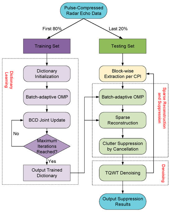
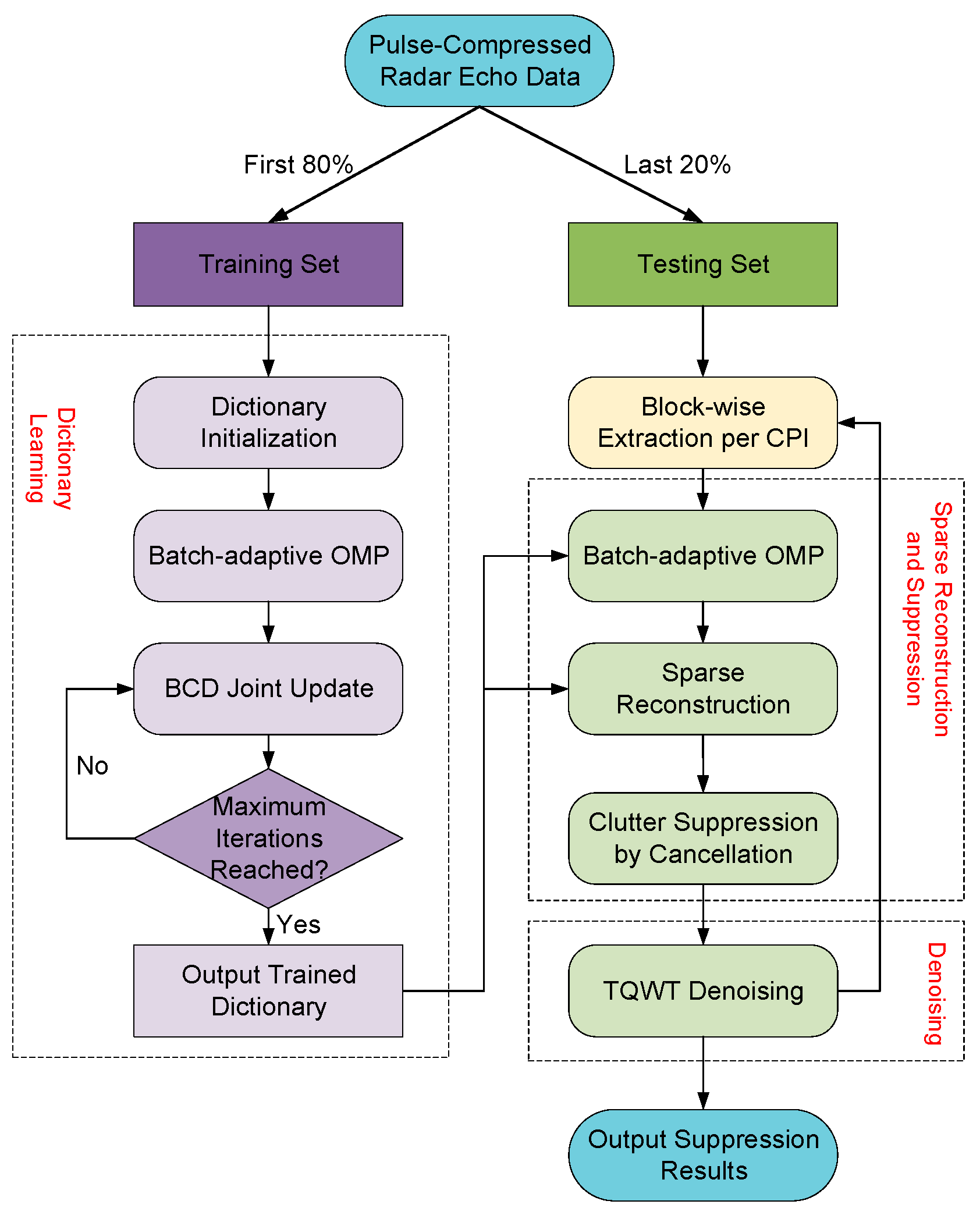
This paper proposes a novel radar sea clutter suppression algorithm that integrates BCD to accelerate dictionary learning, a batch-adaptive OMP for efficient sparse coding, and the TQWT for robust denoising. As illustrated in Figure 1, the overall workflow comprises four primary stages: data preprocessing, dictionary learning, sparse reconstruction-based clutter suppression, and secondary denoising. First, let the pulse-compressed complex radar echoes be arranged as a data matrix , where Np denotes the number of slow-time pulses and M is the number of range cells; each column of S thus corresponds to the slow-time sequence of one range cell. Along the slow-time dimension, the first 80% of the pulses are used to construct the training set, while the remaining 20% form the testing set. To construct pure sea clutter training samples, the range cells containing the target signal are deliberately excluded from the training set.
Figure 1.
Overall flowchart of the proposed sea clutter suppression method.
Second, during the dictionary learning phase, an initial dictionary is initialized using randomly selected training samples, and the corresponding sparse coefficients are computed via the batch-adaptive OMP algorithm. Subsequently, the explicit closed-form analytical solution derived from the BCD algorithm is utilized to provide a precise initial estimation for the dictionary atoms. This is followed by an iterative joint optimization of both the dictionary atoms and the sparse coefficients, ultimately yielding an optimized, domain-specific sea clutter dictionary. Crucially, the introduction of the BCD optimization framework successfully circumvents the high-complexity global SVD required by traditional methods, significantly accelerating the training process. Meanwhile, by deriving the closed-form solution in the complex domain, the algorithm preserves the coherent phase information, thereby retaining the valuable signal characteristics for subsequent processing.
Third, in the sparse reconstruction and clutter suppression stage, the test data (the last 20%) is partitioned and processed frame-by-frame based on the Coherent Processing Interval (CPI). At this stage, the learned dictionary is applied to the test pulses of all range cells, including the target-present cells that were excluded during training, so that the target can be revealed after clutter cancellation. Specifically, the batch-adaptive OMP algorithm sparsely reconstructs the sea clutter components within each CPI, which are then subtracted from the raw echoes to accomplish preliminary clutter suppression. Importantly, because the dictionary is exclusively learned from target-free data, it accurately characterizes the intrinsic slow-time subspace of the sea clutter. Consequently, while the clutter is sparsely reconstructed, the target, which exhibits distinct narrowband features, cannot be effectively represented by the dictionary, and thus its energy is safely preserved after the subtraction. To achieve highly efficient reconstruction at this stage, we integrate global Gram matrix precomputation and a dual-constraint stopping criterion into the batch-adaptive OMP, which drastically eliminates redundant computations when processing large-scale radar echo data.
Finally, in the denoising stage, the TQWT is applied to the preliminarily suppressed signal to filter out residual clutter and background noise. Unlike conventional wavelet transforms, this final block leverages the flexible Q-factor and redundancy of TQWT to effectively characterize the narrowband oscillatory features of weak targets. By effectively removing these residual components without inducing over-smoothing defects, this step significantly enhances the signal-to-clutter-plus-noise ratio (SCNR), thereby yielding a more purified target signal and delivering the final suppression result.
2.2. Training Data Construction
The construction of high-quality, pure sea clutter samples is fundamental to the efficacy of the dictionary learning process [18]. In this paper, the initial 80% of the radar echoes along the slow-time dimension are utilized to construct the training set. To prevent target components from contaminating the dictionary atoms, the range cells containing the target signal are deliberately excluded. Subsequently, the slow-time sequence of each target-free range cell is partitioned along the pulse dimension into non-overlapping segments of length n. Consequently, every training sample represents a length-n slow-time segment drawn from a single range cell, and correspondingly, each dictionary atom is a length-n vector in the slow-time domain. Here, the segment length n is set equal to the length of one CPI, which denotes the number of slow-time pulses jointly processed within a single frame. Within one CPI, the sea clutter is assumed to be approximately stationary.
The segments extracted from all target-free range cells are then collected to form a candidate pool. Furthermore, to mitigate the adverse effects of the direct current (DC) component on the subsequent sparse representation, a zero-mean operation is uniformly applied to all segments. Finally, balancing the generalization capability of the learned dictionary against the computational complexity of the algorithm, L samples are randomly selected from this massive candidate pool to construct the final dictionary training set. This strategic sampling not only decouples the training complexity from the total dataset size, but also prevents the dictionary from overfitting to highly redundant local noise artifacts. The resulting training sample matrix has a dimension of n × L.
2.3. BCD-Accelerated Dictionary Learning
Dictionary learning is a highly effective signal representation technique that adaptively learns a complete or overcomplete dictionary matrix from a given dataset, enabling each signal to be sparsely reconstructed as a linear combination of a few dictionary atoms [19,20,21]. Compared to traditional fixed bases, a data-driven dictionary can more accurately capture the intrinsic physical structures and discriminative features of radar signals [22,23].
Let denote the training data matrix, which comprises L complex-valued pure sea clutter samples of length n. The core objective of dictionary learning is to jointly optimize the dictionary matrix and the corresponding sparse coefficient matrix , such that each training sample can be approximately represented as , , where the coefficient vector is strictly sparse (i.e., containing only a small number of non-zero elements). The K columns of D are the dictionary atoms, i.e., n-dimensional column vectors in the slow-time domain; here, K denotes the number of atoms, and K > n yields an overcomplete dictionary. Because the direct minimization involving the strict -norm constraint leads to a non-convex, NP-hard optimization problem, it is commonly replaced by its convex relaxation, the -norm [24,25]. Consequently, the regularized objective function is expressed as [26]:
where denotes the Frobenius norm, is the initial regularization parameter controlling the sparsity, , and the constraint typically requires each column of the dictionary (i.e., every dictionary atom) to have a unit -norm.
To preserve coherent phase information, this paper extends the dictionary learning framework to the complex-valued domain. Concurrently, to circumvent the high computational burden of traditional global SVD, we introduce a BCD optimization strategy. This strategy requires only a single batch sparse coding operation during the initial phase, after which rapid initial estimation of dictionary atoms is achieved through the closed-form solution derived from two precomputed auxiliary matrices. By employing a complex-valued soft-thresholding operator, the dictionary atoms and the sparse coefficients are then jointly updated. This approach effectively circumvents the redundant computations associated with SVD and repetitive sparse coding, thereby significantly enhancing the overall algorithmic efficiency.
Within the BCD framework, to strictly preserve the sparsity constraint, the joint update of the dictionary and coefficients is restricted solely to the subset of training samples associated with the current atom (i.e., those samples whose sparse representations involve a non-zero coefficient for this specific atom). The residual matrix , obtained by excluding the contribution of the k-th atom and its corresponding sparse coefficient row vector , is defined as [27,28]:
where denotes the i-th column of the dictionary matrix D, represents the conjugate transpose operator, and corresponds to the i-th row vector of the sparse coefficient matrix X. By integrating this residual formulation with an adaptive sparsity regularization strategy, the objective function of the k-th sub-problem, aimed at jointly updating the k-th atom and its non-zero coefficients, can be formulated as:
where is a diagonal matrix controlling the sparsity, with its diagonal elements adaptively determined by (where is the initial regularization parameter defined in Equation (1), is the empirically determined adaptation exponent, and is a small positive constant to ensure numerical stability), and c represents a generic constant. By fixing the sparse coefficient vector to estimate the atom , computing the Wirtinger derivative with respect to in the complex-valued domain and setting it to zero yields:
To alleviate the computational burden and circumvent the repeated calculation of the large residual matrix in each iteration, two precomputed auxiliary matrices are defined as and . Let and denote the k-th columns of A and B, respectively. Accordingly, the numerator of Equation (4) can be reformulated as:
Note that the k-th diagonal element of matrix A satisfies . By substituting this relationship into Equation (4), the direction of the new atom (since dictionary atoms are constrained to have a unit -norm, they essentially represent directional unit vectors in the feature space) can be efficiently estimated using its counterpart from the previous iteration [19]:
Once the initial estimate is obtained, Equation (7) is employed to alternately perform -normalization on the complex-valued dictionary atoms and soft-thresholding updates on the complex-valued sparse coefficients [15]. This alternating process continues until the objective function converges:
The workflow of the proposed BCD-accelerated dictionary learning algorithm is summarized as follows:
- Dictionary initialization: K samples are randomly selected from a target-free sea clutter training set and normalized to initialize the complex-valued dictionary matrix D.
- Initial sparse coding: The batch-adaptive OMP algorithm is employed to compute the initial complex-valued sparse coefficients for all training signals, yielding the coefficient matrix X.
- Initial estimation of dictionary atoms and joint update: First, the auxiliary matrices A and B are computed and cached. For each atom , an initial BCD estimate of the dictionary atom’s direction is evaluated via Equation (6). Subsequently, the adaptive penalty term is calculated based on the coefficient energy, followed by a joint update of the individual atom and its corresponding coefficient row using Equation (7).
- Dictionary pruning and iteration termination: To maintain the representation capacity of the dictionary, any atom that is rarely utilized by the training samples or exhibits high mutual coherence with other atoms is replaced by the sample with the largest current reconstruction error. This pruning of redundant and underutilized atoms is executed at predefined intervals. Steps 3 and 4 are iteratively alternated until the maximum number of iterations is reached. Ultimately, the algorithm outputs the well-trained complex-valued clutter dictionary.
It is worth emphasizing that the four steps above delineate the specific modifications introduced by the proposed BCD-accelerated framework relative to the classical K-SVD algorithm; instead of re-running global sparse coding at every outer iteration and updating each atom through an explicit SVD of the residual matrix, the proposed scheme performs the batch sparse coding only once at the initialization stage (Step 2) and replaces the costly SVD with a closed-form BCD initialization (Equation (6)) followed by an adaptive complex-valued soft-thresholding joint update of each atom and its coefficient row (Equation (7)), as detailed in Step 3.
2.4. Sparse Reconstruction via Batch-Adaptive OMP
The classical OMP algorithm suffers from significant computational overhead when processing massive radar echo data [29,30]. To overcome this limitation, this paper proposes a batch-adaptive OMP algorithm. Specifically tailored for complex-valued sea clutter, this algorithm achieves improvements in both computational efficiency and reconstruction fidelity through the following optimizations.
Regarding computational acceleration, the batch processing mechanism is realized by globally precomputing the Gram matrix and projection matrices, alongside replacing the conventional QR decomposition with an incremental Cholesky factorization. This strategy effectively eliminates the redundant inner-product operations inherent in standard single-vector OMP algorithms, thereby minimizing the computational overhead per iteration [14,31]. For accuracy control, a dual-constraint criterion—governed by a maximum sparsity limit and a dynamic error threshold derived from the signal’s intrinsic energy—is established. Coupled with a progressive threshold-tightening strategy and an early termination mechanism based on residual energy decay, this approach enables flexible sparsity control. Consequently, it effectively prevents overfitting and the selection of spurious dictionary atoms, particularly in scenarios with low SCNR. Ultimately, the proposed algorithm guarantees high-fidelity sparse representations while substantially boosting computational efficiency for large-scale radar signal processing. The detailed procedure of the proposed batch-adaptive OMP algorithm is summarized in Algorithm 1.
| Algorithm 1 Batch-adaptive OMP Algorithm |
| Input: sea clutter dictionary (column-normalized), signal matrix , RMS error goal , maximum sparsity |
| Output: sparse coefficient matrix |
| 1: |
| 2: for to do |
| 3: |
| 4: |
| 5: while and do |
| 6: |
| 7: |
| 8: if then |
| 9: |
| 10: else |
| 11: |
| 12: |
| 13: end if |
| 14: |
| 15: |
| 16: if and then |
| 17: |
| 18: break |
| 19: end if |
| 20: |
| 21: |
| 22: end while |
| 23: |
| 24: end for |
| 25: return |
2.5. TQWT Cascaded Denoising
Due to intrinsic structural differences, dictionary learning can only suppress structured sea clutter. Unstructured thermal noise, which is inevitable in radar signals, lacks correlation and cannot be sparsely represented by the dictionary. Therefore, an additional denoising module is fundamentally required after preliminary clutter suppression. Crucially, this cascaded processing order is irreversible: if denoising were attempted initially, the overwhelming energy of the clutter would severely corrupt the noise variance estimation. Consequently, the TQWT is applied to filter out residual clutter and background noise.
Compared to traditional wavelet transforms, TQWT achieves flexible frequency-band partitioning by independently adjusting its quality factor (Q-factor) and redundancy [32,33,34]. Its superior capability to characterize narrowband oscillatory features perfectly aligns with the physical behavior in the slow-time domain of weak target echoes embedded in a sea clutter background. Furthermore, the adjustable redundancy endows the transform with highly desired shift-invariance, which effectively mitigates the Gibbs phenomenon commonly encountered during signal reconstruction.
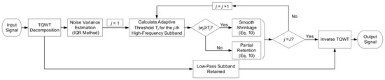
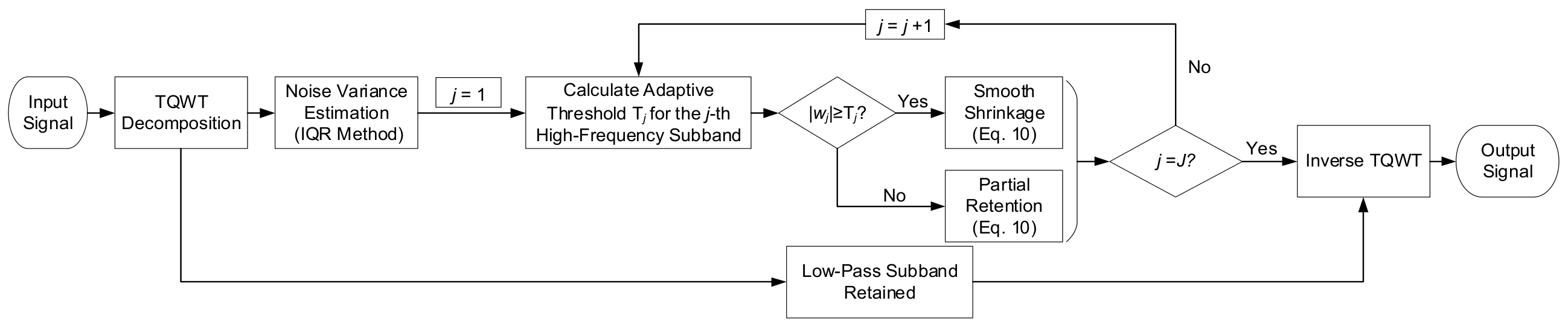
Motivated by these advantages, this paper designs a multi-scale TQWT-based denoising algorithm. The core processing workflow, as illustrated in Figure 2, proceeds as follows: First, the TQWT is applied to perform multiscale decomposition on the clutter-suppressed residual signal. Considering that random noise is predominantly concentrated in the high-frequency spectrum [35,36], the algorithm extracts the coefficients from the first high-frequency subband. Subsequently, the interquartile range (IQR) method is applied to these coefficients to robustly estimate the background noise level , thereby effectively mitigating the estimation bias caused by target outliers [37]:
where and denote the 25th and 75th percentiles of the coefficient distribution within the first high-frequency subband, respectively.
Figure 2.
Flowchart of the TQWT denoising algorithm.
Subsequently, for the j-th high-frequency subband (j = 1, 2, …, J, where J denotes the total number of high-frequency subbands), given that the noise magnitude typically decays progressively as the decomposition level increases, a scale-dependent adjustment factor is incorporated into the universal threshold [15]. This yields the adaptive threshold corresponding to each high-frequency subband:
where N denotes the length of the input signal. Once the adaptive thresholds are determined, the algorithm preserves the low-pass subband intact, while employing a continuously differentiable smooth thresholding function to nonlinearly shrink the high-frequency subband coefficients at each decomposition level [15]:
where denotes the original high-frequency wavelet coefficient, represents the adaptive threshold of the current decomposition level, stands for the processed wavelet coefficient, and the parameters , , and are tuning factors. Equation (10) formulates a piecewise thresholding mechanism, where an exponential-based smooth shrinkage function is applied to coefficients exceeding or equal to the threshold for robust noise suppression. Conversely, for coefficients below the threshold, a retention factor is introduced to preserve local details that may contain ultra-weak target components. Finally, the shrunken high-frequency coefficients and the unaltered low-frequency subband are fed into the inverse TQWT, reconstructing the time-domain signal and yielding the final denoised output.
In conclusion, the proposed algorithm seamlessly integrates the exceptional weak-oscillatory-feature extraction capability of the TQWT with a sophisticated smooth shrinkage strategy. This synergy not only overcomes the pseudo-Gibbs artifacts commonly induced by traditional hard thresholding and the over-smoothing defects inherent in soft thresholding, but also maximizes the preservation of authentic target echoes against severe sea clutter backgrounds. Consequently, it lays a robust foundation for the reliability of subsequent radar target detection.
3. Datasets and Experimental Results
3.1. Real-Measured Radar Datasets
To demonstrate the efficacy of the proposed method, experimental validations were performed on two widely adopted measured radar datasets: the IPIX dataset, acquired by McMaster University, Canada, in 1993, and a recently published sea clutter dataset from the Journal of Radars. Characterized by small-target echoes embedded in severe authentic sea clutter, both datasets serve as highly representative benchmarks for maritime radar signal processing.
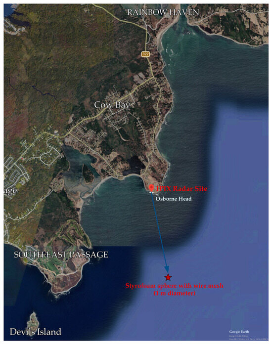
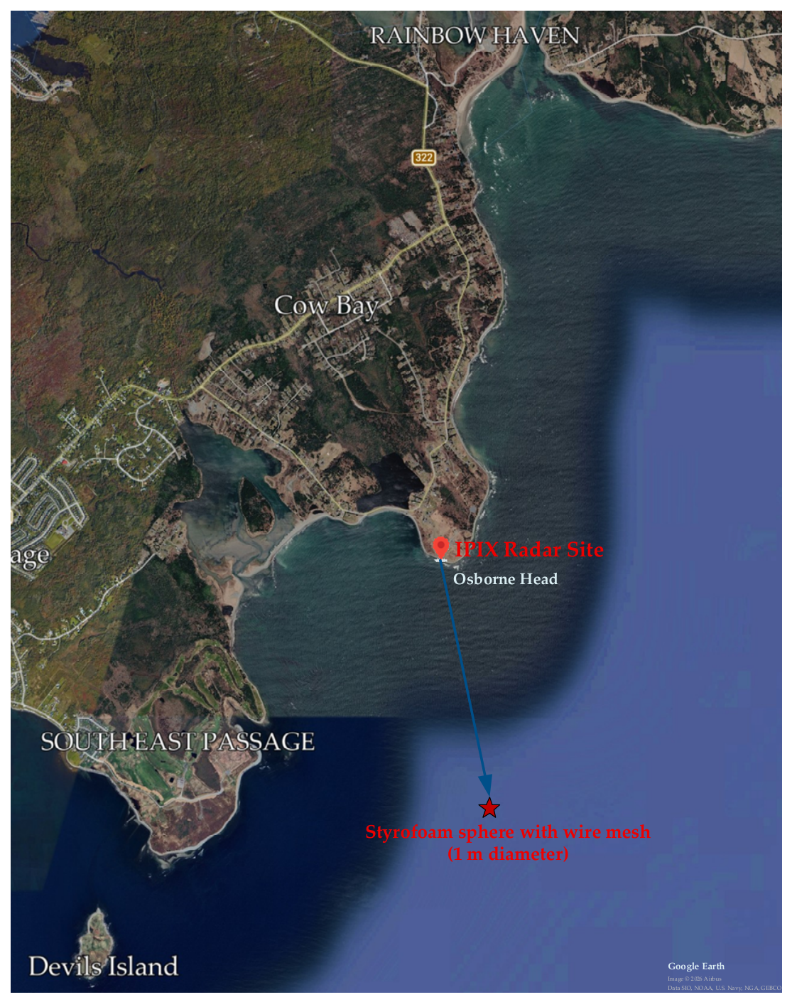
The IPIX dataset was collected by an X-band fully coherent radar deployed on a clifftop near Dartmouth, Nova Scotia, on Canada’s east coast. The geometry of the experimental scenario is illustrated in Figure 3. For performance validation, this paper utilizes data file #280 (hereafter denoted as Dataset 1), which records radar echoes under Sea State 3 conditions. The dataset consists of 14 range cells with 131,072 pulses per cell. Among the four available polarization channels (HH, VV, HV, and VH), the HH-polarized data is utilized for the primary algorithmic evaluation, while the remaining channels are subsequently employed to comprehensively validate the generalization capability of the proposed method under varying polarization mechanisms. During the data collection, a spherical target (a 1 m-diameter styrofoam ball wrapped with wire mesh) was deployed at the 8th range cell. Because target scattering energy spills over into neighboring range cells, range cells 7–10 are masked out as the target-present region. The remaining range bins, therefore, are well-suited for extracting pure sea clutter training samples.
Figure 3.
Map of the experimental site for the IPIX radar dataset near Dartmouth, Nova Scotia.
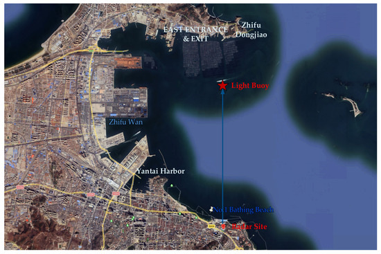
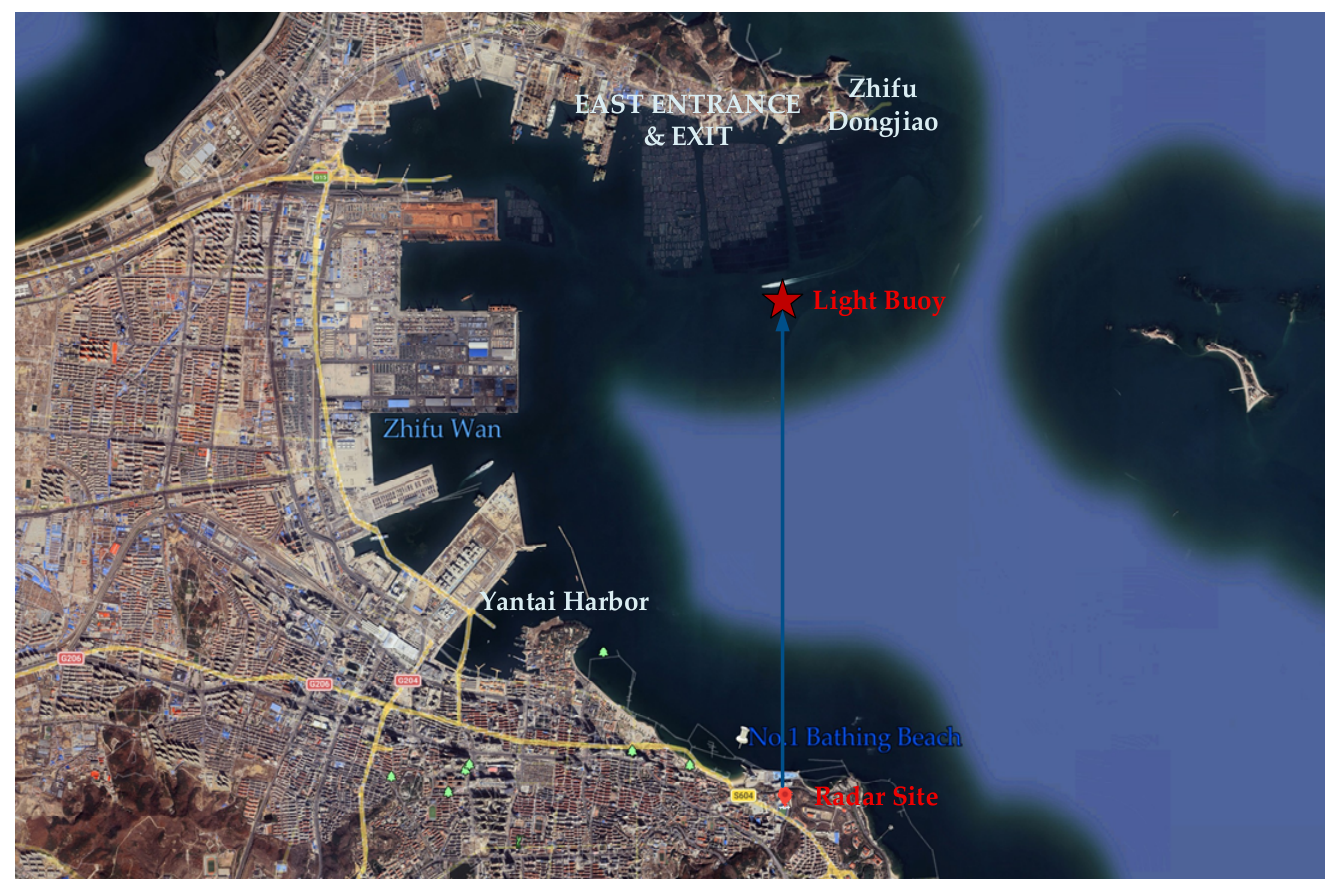
Sourced from the open-access dataset platform of the Journal of Radars, the second dataset was acquired using a Tian’ao SPPR50P X-band radar deployed at the Yantai First Seawater Bathing Beach coastal site (Yantai, China), as illustrated in Figure 4. In this paper, the data file “20221113090050_stare_HH”, designated as Dataset 2, is selected for experimental validation. Recorded under Sea State 4 conditions, the T2 channel contains 1000 range cells, of which cells 496–508 encompass the radar returns from a single light buoy moored 2.97 nautical miles away. The first 12,800 pulses of this file are extracted for analysis, yielding an effective observation window of 6.4 s. Compared to the IPIX dataset, Dataset 2 features a higher pulse repetition frequency (PRF), finer range resolution, and substantially more complex sea clutter dynamics, thereby posing a greater challenge for clutter suppression. The inclusion of two datasets with distinct parameter configurations and sea state conditions is intended to validate the generalization capability and robustness of the proposed algorithm across diverse operational scenarios. A comprehensive comparison of the key technical specifications between the two datasets is detailed in Table 1.
Figure 4.
Map of the experimental site at Yantai First Seawater Bathing Beach.
Table 1.
Comparison of main technical parameters between the IPIX and Journal of Radars datasets.
3.2. Performance Evaluation Metrics
To quantitatively validate the proposed method, distinct metrics are adopted for different processing stages. During the training phase, Peak Signal-to-Noise Ratio (PSNR) and Mean Similarity () are employed to assess the representational capacity of the learned dictionary and the fidelity of sea clutter reconstruction. In the testing phase, the SCNR improvement (ΔSCNR) serves as the primary criterion to evaluate the clutter suppression performance of the proposed algorithm.
3.2.1. Peak Signal-to-Noise Ratio (PSNR)
PSNR, a quantitative metric derived from the Mean Squared Error (MSE), is employed to evaluate the global reconstruction fidelity of the learned dictionary across the entire training dataset. A higher PSNR indicates a lower overall reconstruction error, demonstrating the superior representational capacity of the learned dictionary for the complex-valued, target-free sea clutter data. Mathematically, the PSNR is defined as follows:
where the MSE of the complex-valued matrix is calculated by:
In these expressions, denote the original target-free sea clutter training matrix and the corresponding matrix reconstructed by the learned dictionary, respectively; and are their respective entries. The term represents the global peak amplitude across the entire original training matrix.
3.2.2. Mean Similarity Metric ()
To evaluate the coherence between each individual training sample and its reconstructed counterpart , a similarity metric is introduced [16,21]. First, their discrete cross-correlation sequence is computed as follows:
where denotes the complex conjugate. The sequence is subsequently normalized by the signal energies:
where and represent the auto-correlation at zero lag, equating to the energies of the original and reconstructed signals, respectively. Accordingly, the similarity metric for the i-th sample is defined as the maximum absolute value of the normalized cross-correlation sequence:
Finally, the mean similarity over the entire training set is calculated as the arithmetic mean of all individual sample similarities:
where L is the total number of training samples. A mean similarity closer to unity implies a stronger correspondence between the reconstructed and the original signals, which further demonstrates that the learned dictionary can effectively capture and preserve the intrinsic structural characteristics of the sea clutter.
3.2.3. SCNR Improvement (ΔSCNR)
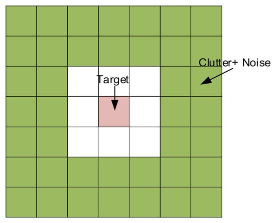
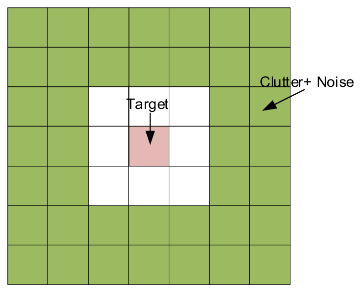
To quantitatively evaluate the algorithm’s clutter suppression performance within each CPI, the SCNR is computed in the range-Doppler (RD) domain before and after clutter suppression. As illustrated in Figure 5, the target power, denoted as , is defined as the peak power within the predetermined target region. Conversely, the average power of the area outside the target region is taken as the background clutter-plus-noise power, denoted as . Thus, the SCNR is calculated as:
Figure 5.
Schematic diagram of the target and background region partition in the RD domain for SCNR calculation.
Subsequently, the SCNR improvement (ΔSCNR) is determined by calculating the difference between the output and input SCNR values:
A larger positive ΔSCNR value indicates more effective clutter suppression, thereby providing a more advantageous condition for subsequent target detection tasks.
3.3. Experimental Results on the IPIX Dataset
To validate the performance of the proposed algorithm under real-world sea conditions, experiments are initially conducted using the HH-polarized data from Dataset 1. The pulse-compressed radar echo data is partitioned into training and testing sets at an 8:2 ratio. Subsequently, 5000 pure clutter samples of length n = 64 (corresponding to the number of pulses within a single CPI) are randomly extracted from the training set for dictionary learning. Here, the CPI length is set a priori to 64, which is a standard empirical value in radar signal processing. This choice ensures computational efficiency while satisfying the physical requirement that sea clutter remains approximately stationary within this short observation window. To achieve a reasonable trade-off between reconstruction fidelity and overfitting prevention, the number of dictionary atoms K is set to 80, the number of learning iterations is configured to 50, and the initial regularization parameter is defined as 0.5. For the batch-adaptive OMP stage, the maximum sparsity level is constrained to . Furthermore, to mitigate the impact of random sample selection, the entire experimental procedure is independently repeated five times, and the average values are taken as the final results.
During the training phase, the proposed BCD-accelerated algorithm is employed to perform dictionary learning on the training matrix. Quantitative evaluations averaged over five trials demonstrate that the overall PSNR of the reconstructed pure sea clutter in the training set achieves 37.80 dB, accompanied by a mean similarity of 0.89. These metrics indicate that the learned dictionary can accurately capture the principal structural features of the complex-valued sea clutter, thereby enabling high-fidelity sparse reconstruction of the clutter components.
During the testing phase, the batch-adaptive OMP algorithm is employed in conjunction with the learned dictionary to perform sparse coding on each CPI of the testing set. This procedure accurately reconstructs the sea clutter component, which is subsequently subtracted from the original radar echo to achieve preliminary clutter suppression. Finally, the TQWT denoising algorithm is applied to the residual signal to mitigate non-stationary residual clutter and background thermal noise, thereby yielding superior overall clutter suppression performance.
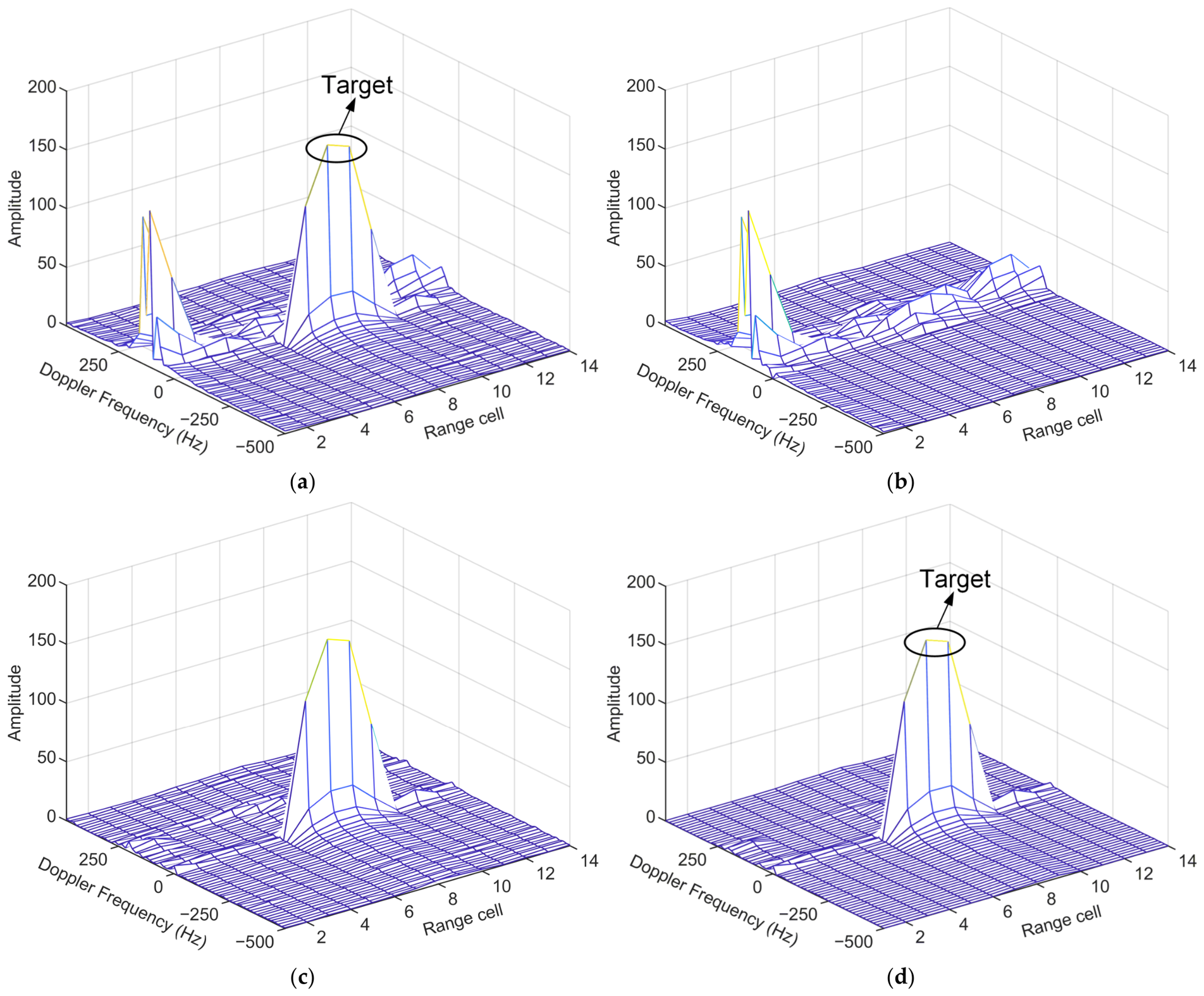
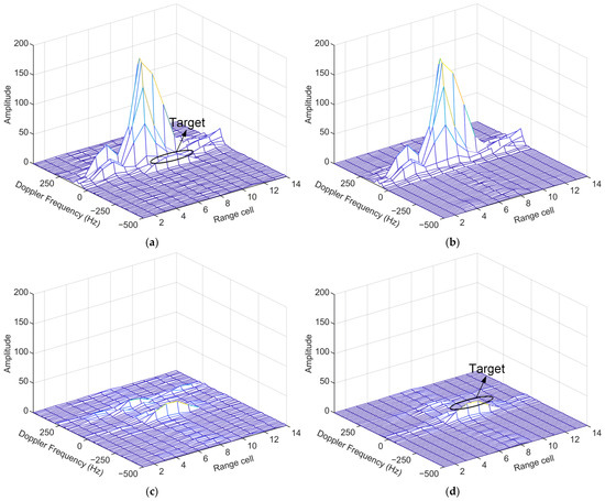
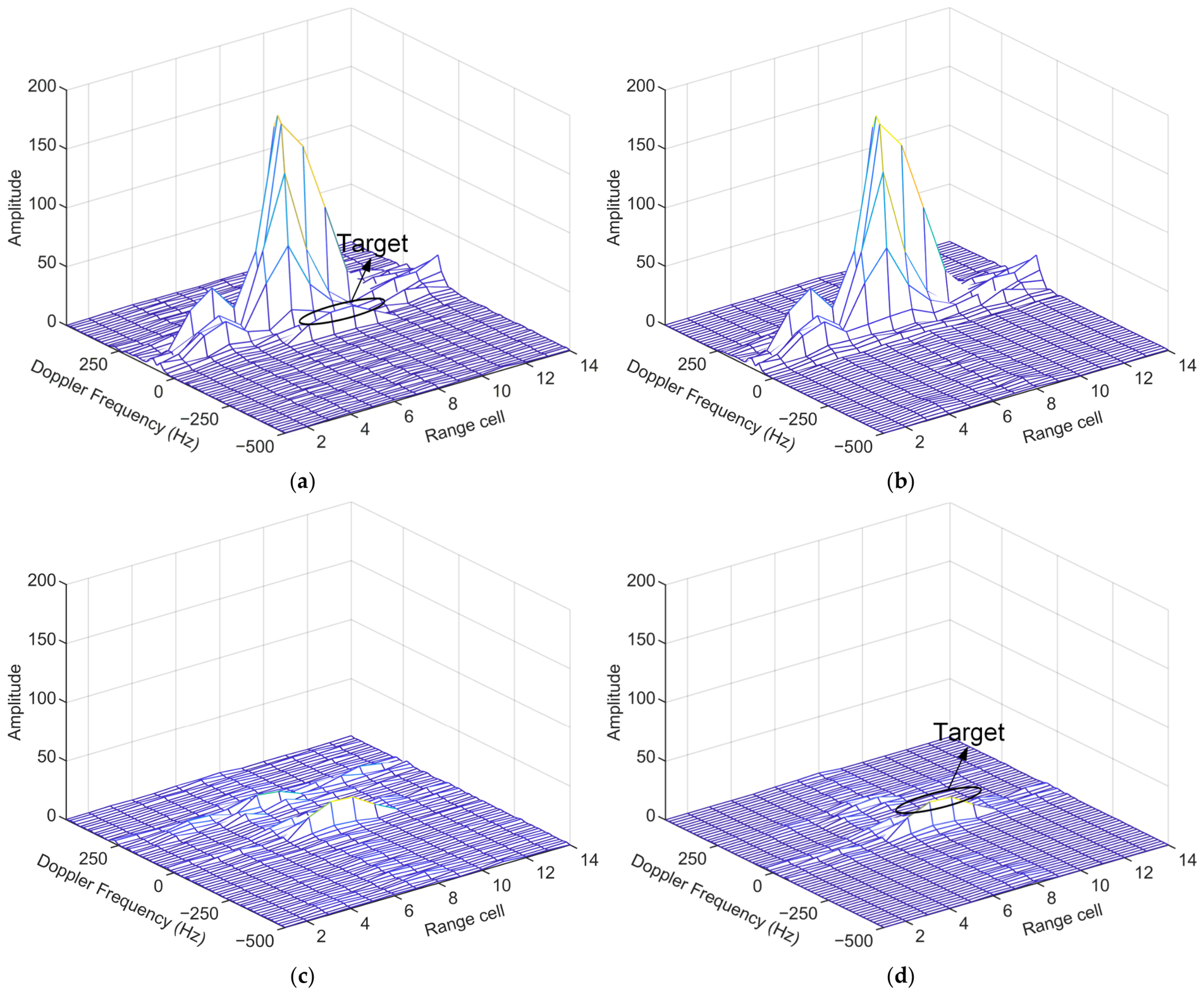
As a representative visual example from one of the five independent trials, Figure 6 illustrates the 3D RD spectral processing results for CPI 18 from the test set of Dataset 1, which represents a high-input SCNR condition of 25.33 dB. In the original RD map (Figure 6a), the sea clutter is offset from the zero-Doppler axis. Although the radar platform is stationary, the wind-driven drift and orbital motion of the sea surface impart radial velocities to the clutter scatterers, shifting the clutter spectrum away from 0 Hz. Owing to the distribution of these radial velocities, the sea clutter generally spans a wider Doppler extent than the narrowband target echo. A comparison within Figure 6a,b reveals that the proposed algorithm faithfully reconstructs the pure sea clutter component while successfully avoiding the erroneous reconstruction of the target signal. Subsequently, after the cancellation procedure (Figure 6c), the background clutter energy is significantly diminished, yet the target peak remains effectively preserved. Finally, the application of the TQWT denoising algorithm (Figure 6d) further mitigates the non-stationary residual clutter and background thermal noise. Overall, the cascaded processing pipeline significantly flattens the background baseline of the RD spectrum and accentuates the target peak, thereby demonstrating superior clutter suppression and improved target detectability.
Figure 6.
3D RD spectral plots at various processing stages for CPI 18 from the test set of Dataset 1 under a high-input SCNR (25.33 dB): (a) Original RD map; (b) Reconstructed RD map; (c) RD map after preliminary clutter suppression; (d) Denoised RD map.
To verify the robustness of the proposed method under more challenging conditions, CPI 256 from the same test set, characterized by a profoundly low input SCNR of 1.64 dB, is further selected for evaluation. As illustrated in Figure 7a, the weak target is almost entirely buried within the severe sea clutter, rendering direct detection highly difficult. Following the dictionary-based reconstruction and clutter cancellation procedures (Figure 7b,c), although the target peak becomes discernible, a substantial amount of non-stationary residual clutter and background noise persists, which inherently increases the risk of false alarms.
Figure 7.
3D RD spectral plots at various processing stages for CPI 256 from the test set of Dataset 1 under a low input SCNR (1.64 dB): (a) Original RD map; (b) Reconstructed RD map; (c) RD map after preliminary clutter suppression; (d) Denoised RD map.
To address this persistent issue, the TQWT algorithm is subsequently applied to perform further denoising on the residual signal (Figure 7d). Through this procedure, the residual clutter and noise are effectively filtered out, yielding a distinctly flattened background baseline and a highly prominent target peak. Following the complete cascaded processing pipeline, the output SCNR reaches 28.32 dB, achieving a substantial improvement of 26.68 dB. Both the qualitative spectral comparisons and the significant improvements in quantitative metrics compellingly demonstrate that the proposed method possesses exceptional sea clutter suppression capabilities and robust weak target detectability, even under extremely low SCNR conditions.
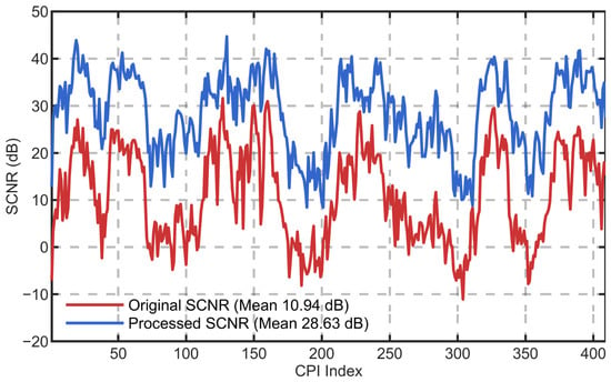
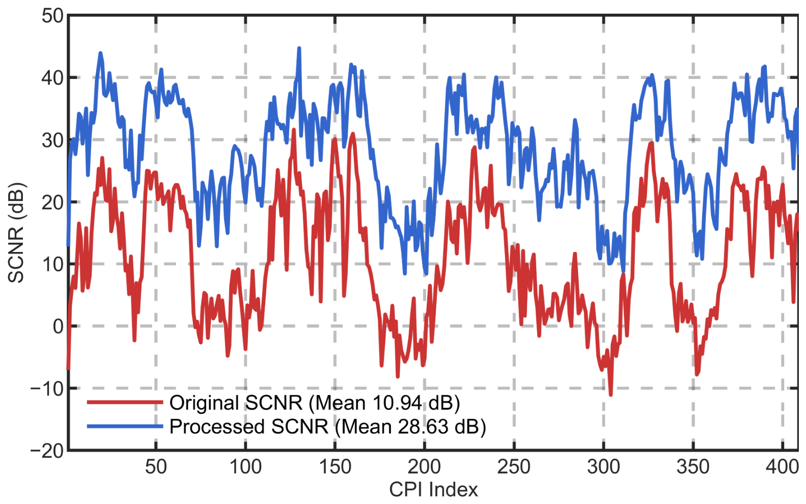
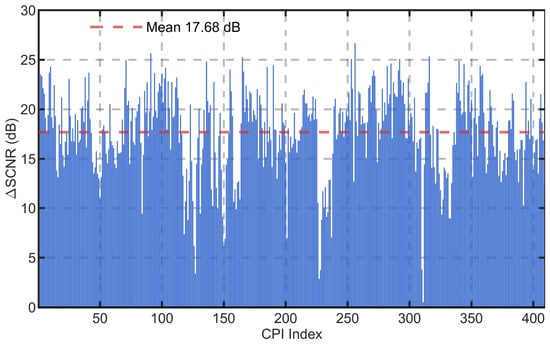
To comprehensively evaluate the robustness and effectiveness of the proposed method in continuous observation scenarios, the SCNR and its corresponding improvement (ΔSCNR) were calculated for all CPIs in the test set before and after clutter suppression. The quantitative results are presented in Figure 8 and Figure 9.
Figure 8.
Comparison of SCNR before and after processing for all tested CPIs from Dataset 1.
Figure 9.
SCNR improvement (ΔSCNR) across all tested CPIs from Dataset 1.
As illustrated in Figure 8, the SCNR of the original data fluctuates significantly and remains at a relatively low level overall, yielding a mean value of merely 10.94 dB. Following processing by the proposed method, the SCNR for each tested CPI exhibits a substantial and consistent enhancement, elevating the mean value to 28.63 dB. Furthermore, the distribution of ΔSCNR values in Figure 9 demonstrates that the algorithm achieves a 100% positive SCNR gain (ΔSCNR > 0) across the entire test set, securing an overall average improvement of 17.68 dB. Notably, only five CPIs yield an improvement slightly below 5 dB, indicating that 98.8% of the evaluated CPIs acquire a substantial performance gain exceeding 5 dB.
Collectively, the experimental results presented above demonstrate that the proposed method exhibits superior and robust sea clutter suppression performance across diverse CPI conditions. By significantly elevating the output SCNR, this algorithm lays a reliable foundation for subsequent CFAR detection and the stable tracking of weak maritime targets.
3.4. Experimental Results on the Journal of Radars Dataset
To further validate the generalization capability and robustness of the proposed method under complex sea conditions and across distinct datasets, experiments were conducted using a continuous observation interval of 12,800 pulses from Dataset 2 (Channel T2). These data were collected in Sea State 4 and encompass 1000 range cells, with the actual target located between range cells 496 and 508. To ensure the fairness of the evaluation, all algorithmic parameters were kept strictly consistent with those utilized in the IPIX experiments.
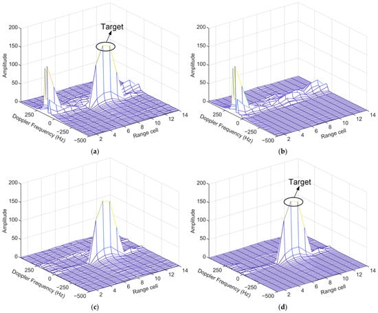
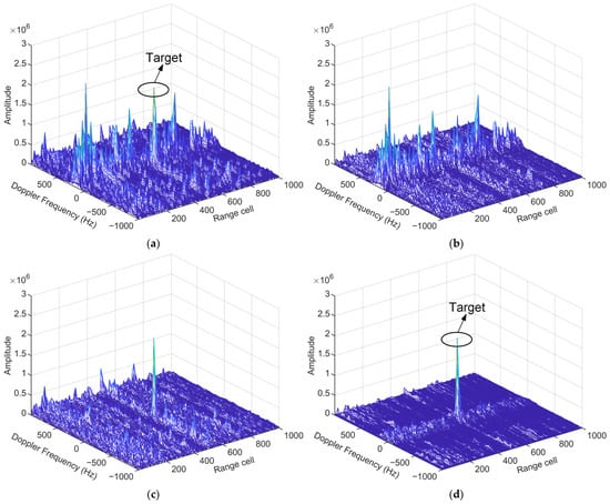
Figure 10 illustrates the evolution of the 3D RD spectrum for CPI 21 from the test set of Dataset 2. As shown in Figure 10a, under Sea State 4 conditions, the raw data contain numerous high-intensity sea spikes, which severely mask weak targets and elevate the false alarm rate. Following reconstruction and preliminary clutter cancellation via the proposed method (Figure 10b,c), the vast majority of sea spikes are effectively suppressed, rendering the target preliminarily visible. Subsequently, the TQWT-based denoising module is employed to filter out residual clutter and noise. As depicted in the final output in Figure 10d, the background of the RD spectrum is significantly flattened, and the target peak is highly prominent, exhibiting a substantially elevated SCNR. This visual evidence compellingly demonstrates that the proposed algorithm maintains excellent resistance to sea spike interference and preserves superior weak target detection capabilities across distinct datasets and complex sea conditions.
Figure 10.
3D RD spectral plots at various processing stages for CPI 21 from the test set of Dataset 2: (a) Original RD map; (b) Reconstructed RD map; (c) RD map after preliminary clutter suppression; (d) Denoised RD map.
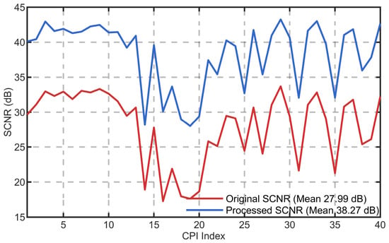
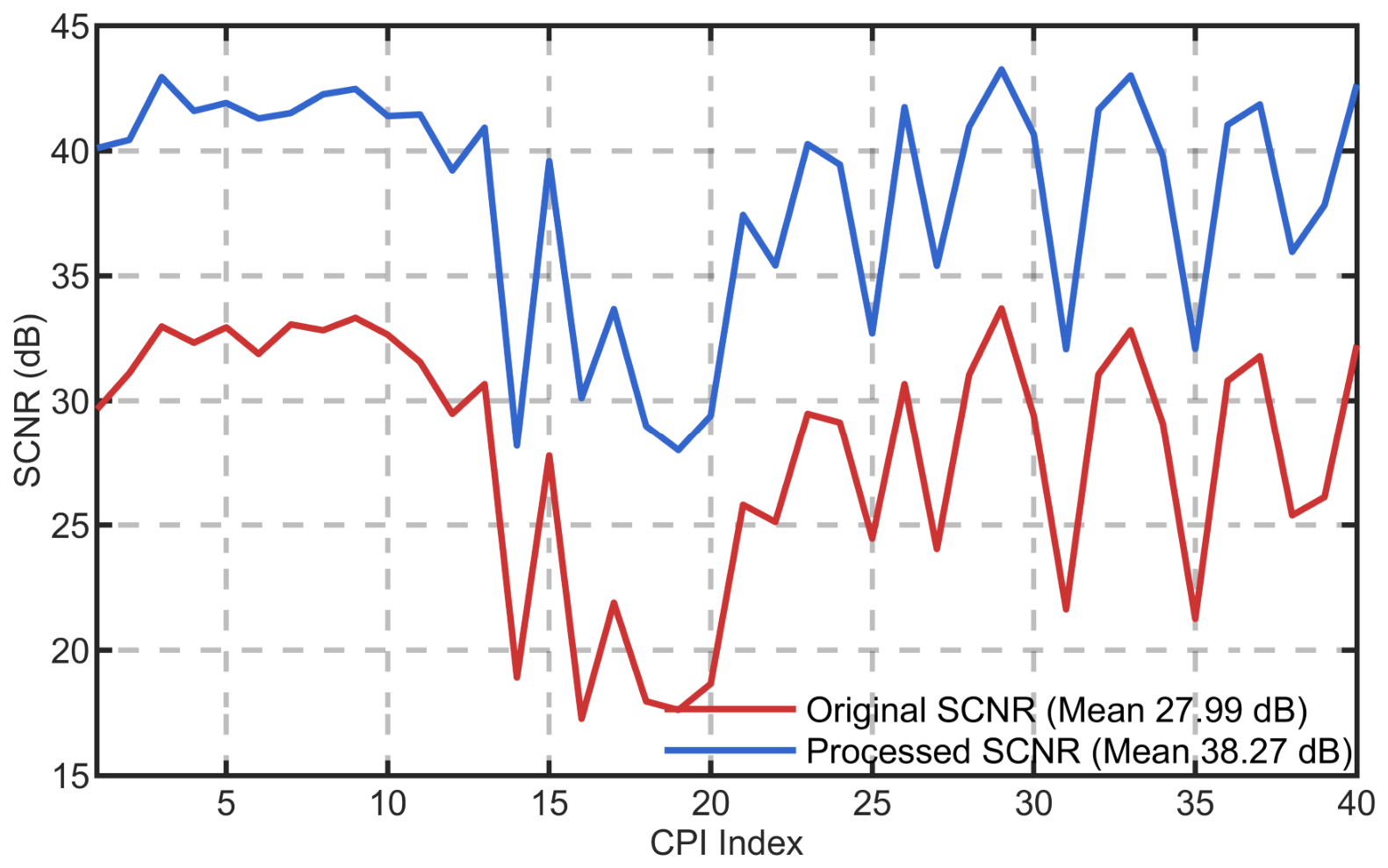
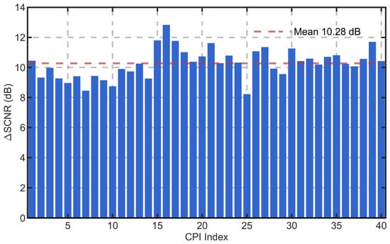
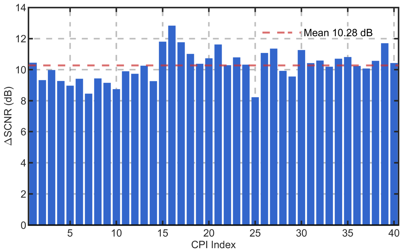
To evaluate the proposed method’s clutter suppression performance across consecutive observation CPIs in Dataset 2, Figure 11 and Figure 12 present the input and output SCNR values, alongside the corresponding SCNR improvement (ΔSCNR), for all 40 tested CPIs.
Figure 11.
Comparison of SCNR before and after processing for all tested CPIs from Dataset 2.
Figure 12.
SCNR improvement (ΔSCNR) across all tested CPIs from Dataset 2.
As illustrated in Figure 11, due to the severe sea spikes induced by rough sea conditions, the SCNR of the raw data exhibits significant fluctuations, yielding a mean of merely 27.99 dB. Following processing via the proposed method, the output SCNR curve demonstrates a consistent and substantial enhancement, with the mean value elevating significantly to 38.27 dB. Furthermore, the bar chart in Figure 12 indicates that all 40 tested CPIs achieved a 100% positive performance gain (ΔSCNR > 0), securing an overall average ΔSCNR of 10.28 dB. These quantitative results compellingly reaffirm that the proposed method possesses excellent generalization capability and robustness when mitigating severe sea spike interference during the continuous processing of consecutive CPIs.
3.5. Generalization Analysis Across Different Polarizations
To comprehensively evaluate the generalization capability and robustness of the proposed algorithm across varying radar scattering mechanisms, extended experiments are conducted using all four polarizations (HH, VV, HV, and VH) from Dataset 1. To ensure a rigorous and fair evaluation, all fundamental algorithmic parameters are kept strictly identical across the test cases, with the initial sparsity regularization parameter λ specifically investigated as the core control variable. Furthermore, to mitigate the influence of random factors, five independent trials are performed for each polarization condition. Table 2 summarizes the clutter suppression performance under different polarizations and sparsity penalties. Herein, ΔSCNR (dB) denotes the average SCNR improvement over the five independent trials, and the Positive SCNR Gain Ratio (%) represents the proportion of CPIs in the test set that achieve a positive SCNR improvement.
Table 2.
Clutter suppression performance under different polarizations and sparsity penalties.
As can be observed from the data in Table 2, under identical sparsity regularization parameters, the proposed algorithm demonstrates a certain level of clutter suppression capability across all polarization conditions, although there are noticeable variations in performance. Specifically, in HH polarization, the algorithm achieves the most outstanding clutter suppression effect, where not only does the ΔSCNR reach its maximum, but the Positive SCNR Gain Ratio is also as high as 100%. The performance of cross-polarizations (HV and VH) is suboptimal, yet their positive gain ratios remain above 95%, demonstrating the algorithm’s good robustness against such low-power clutter. In contrast, VV polarization proves to be the most challenging scenario, yielding the lowest ΔSCNR and the highest number of CPIs experiencing negative gains.
Furthermore, examining the impact of the initial sparsity regularization parameter λ reveals the adaptability of the algorithm under different polarization mechanisms. The parameter λ directly controls the strength of the sparsity penalty during dictionary training. When λ is small (e.g., λ = 0.5), the regularization constraint is weaker, granting the dictionary a higher degree of representational freedom and an inclination to precisely fit the subtle details into the training set. Conversely, when λ is larger (e.g., λ = 2), the sparsity penalty is enhanced, compelling the dictionary to learn only the most macroscopic, high-energy dominant components of the clutter, thereby discarding weak details. The comparison reveals that for HH polarization, increasing λ leads to a slight decrease in ΔSCNR. This is primarily because the increased sparsity penalty causes the dictionary to slightly underfit the fine-grained details of the clutter data. Conversely, for VV, HV, and VH polarizations, the clutter suppression performance improves as λ increases. This phenomenon is particularly prominent in VV polarization. A possible explanation is that sea clutter in VV polarization is predominantly caused by Bragg scattering, where the target and clutter share more similar characteristics. If a smaller λ is used, the complex dictionary tends to overfit the training set; it not only learns the clutter features but also acquires the ability to represent target-like signals. Consequently, during the sparse reconstruction phase, the target components are erroneously reconstructed as clutter, which leads to undesired target cancellation during the subtraction process, thereby reducing the ΔSCNR or even causing negative gains. Increasing λ successfully forces the model to ignore these ambiguous details, effectively preserving the target energy. Given that the high coupling between target and clutter in VV polarization makes it the most difficult to suppress, designing an adaptive parameter optimization mechanism tailored for dynamic sea states will be a key focus of our future research.
3.6. Comparative Analysis of Different Clutter Suppression Algorithms
In this section, comparative evaluations are conducted on the HH-polarized data from Dataset 1 to assess both the clutter suppression capabilities and the computational efficiency of the proposed algorithm. The proposed method was benchmarked against classical approaches (i.e., K-SVD and C-KSVD) as well as the recently proposed C-ASJU_ECWT method. For an unbiased evaluation, all common parameters were kept strictly identical across the algorithms. Furthermore, to mitigate the impact of stochastic variations, each method was executed for five independent runs, with the averaged outcomes reported as the final performance metrics. The detailed quantitative results are summarized in Table 3.
Table 3.
Comparison of performance and computational time among the four sea clutter suppression algorithms.
Table 3 presents a comprehensive comparison of the clutter suppression performance and computational efficiency among the four sea clutter suppression algorithms. PSNR and serve as the reconstruction performance metrics during the training phase, while ΔSCNR acts as the crucial metric for evaluating the clutter suppression performance during the testing phase. Furthermore, DL, SR, and Denoising denote the computational time required for dictionary learning, sparse reconstruction alongside the preliminary cancellation of sea clutter, and the denoising module, respectively. Total Time represents the overall runtime, encompassing the aforementioned core modules along with data loading, preprocessing, and other auxiliary procedures such as performance evaluation.
Regarding clutter suppression performance, the proposed method achieves a ΔSCNR of 17.48 dB, which significantly outperforms the conventional K-SVD and C-KSVD approaches, as well as the state-of-the-art C-ASJU_ECWT method. Although the reconstruction PSNR and similarity measure of the proposed algorithm on the pure clutter training set are slightly lower than those of traditional K-SVD variants, this is an intentional parameter design aimed at preventing the dictionary from overfitting to the background clutter. This strategy effectively enhances the algorithm’s generalization capability and robustness when processing real-world radar echoes.
In terms of computational efficiency, the proposed algorithm introduces a BCD strategy during the dictionary training phase to replace the traditional SVD for an accurate initial estimation of dictionary atom directions. This strategy significantly reduces the dictionary learning time to 3.67 s. Compared to the traditional K-SVD and C-KSVD algorithms, which alternately update dictionary atoms and sparse coefficients, this approach substantially alleviates the training overhead. Even when compared to the relatively faster C-ASJU_ECWT algorithm (7.33 s), the dictionary learning efficiency of the proposed method is nearly doubled.
Notably, as shown in Table 3, the proposed algorithm’s time for sparse reconstruction and preliminary cancellation during the testing phase (SR, 0.70 s) is slightly higher than that of the comparative algorithms. Although this paper adopts the batch-adaptive OMP algorithm to accelerate sparse coding, the restricted size of Dataset 1 (containing only 14 range cells and 64 pulses per CPI) prevents it from fully leveraging the advantages of batch matrix operations. In this scenario, the underlying overhead for matrix initialization and memory scheduling actually leads to a slight increase in processing time. To validate this hypothesis, supplementary experiments were conducted on a larger-scale dataset (Dataset 2, where the test set comprises 40 CPIs, each with a dimension of 64 × 1000). The results indicate that the proposed algorithm requires only 3.24 s in the SR stage, which is superior to K-SVD (3.64 s), C-KSVD (3.25 s), and C-ASJU_ECWT (3.27 s). Furthermore, during a single sparse coding test on a large-scale training sample size of 64 × 5000, the proposed algorithm takes merely 0.38 s, outperforming the traditional OMP algorithm (0.47 s) used in the C-ASJU_ECWT method. This supplementary evidence thoroughly demonstrates that as the data matrix dimensions scale up, the computational advantages of batch-adaptive OMP in sea clutter suppression become significantly prominent.
In addition, among the algorithms incorporating a denoising module, the denoising time of the proposed algorithm is 3.31 s, which is higher than the 1.31 s required by C-ASJU_ECWT. This discrepancy primarily stems from the fundamental differences in their underlying processing mechanisms. ECWT leverages two-dimensional wavelet decomposition to perform global processing on the entire slow-time-range data matrix within a CPI. In contrast, as a one-dimensional tunable Q-factor wavelet transform, TQWT is intrinsically designed to characterize the local oscillation features within a 1-D temporal sequence. Consequently, the proposed algorithm necessitates executing independent TQWT decomposition, thresholding, and inverse reconstruction on the echo sequence of each individual range cell, thereby increasing the computational overhead during the denoising stage.
Nevertheless, this cell-by-cell independent processing strategy holds profound physical significance for the final signal purification. It effectively isolates the spatial heterogeneity of residual clutter and background noise across different range cells, preventing the spatial smearing and mutual interference that may arise during 2-D joint processing in the ECWT denoising algorithm. Simultaneously, it is conducive to preserving the local oscillation features of weak targets along the slow-time dimension. As demonstrated in Table 4, although the cascaded TQWT denoising module introduces additional computational time, it drastically elevates the ΔSCNR to 17.48 dB during the testing phase. This result is superior to both the 13.08 dB achieved without a denoising module and the 15.23 dB obtained using the cascaded ECWT denoising module. This supplementary evidence thoroughly demonstrates that the proposed TQWT denoising strategy, by trading off acceptable computational overhead, achieves a substantial enhancement in the ultimate detectability of weak targets.
Table 4.
Ablation study results of the denoising modules in the proposed algorithm.
Overall, the proposed algorithm achieves a total processing time of only 7.99 s in the experiments on Dataset 1, exhibiting the highest computational efficiency among all compared methods. Compared to the conventional K-SVD and C-KSVD algorithms, the total execution time is drastically reduced by approximately 78.9% and 73.8%, respectively. Even when compared to the second-fastest method, C-ASJU_ECWT, the execution time is further reduced by approximately 16.2%. This outstanding performance firmly demonstrates the proposed method’s potential to effectively tackle real-time sea clutter suppression tasks in practical radar systems.
In summary, the proposed method achieves improved generalization at the expense of a minor decrease in reconstruction metrics. By maintaining superior clutter suppression performance while significantly reducing computational overhead, the algorithm successfully achieves a well-balanced trade-off between processing efficacy and computational efficiency.
4. Discussion
The proposed sea clutter suppression framework demonstrates exceptional advantages in both clutter suppression performance and computational efficiency. By cascading BCD-accelerated dictionary learning, batch-adaptive OMP, and TQWT denoising, this study addresses the inherent bottlenecks of traditional dictionary learning and sparse coding algorithms. The results and their broader implications are discussed as follows.
4.1. Mechanisms of Computational Acceleration and Applicability Boundaries
Traditional K-SVD-based dictionary learning algorithms heavily rely on the SVD of the residual matrix to alternately update dictionary atoms and sparse coefficients. However, the immense computational burden introduced by full-matrix SVD and the alternating update mechanism severely limits algorithmic efficiency. Similarly, standard OMP algorithms suffer from massive and redundant vector inner-product calculations. In our study, the BCD strategy is utilized to precisely estimate the initial direction of dictionary atoms. Integrating this with the adaptive soft-thresholding operator facilitates the lightweight, joint update of both the dictionary atoms and sparse coefficients, successfully bypassing the massive time consumption caused by full-matrix SVD and alternating updates. Furthermore, during the sparse reconstruction stage, the introduced batch-adaptive OMP leverages the global precomputation of the dictionary Gram matrix and incremental Cholesky decomposition, significantly alleviating the computational burden of processing radar echoes.
However, it must be clarified that the acceleration mechanism of the batch-adaptive OMP has specific applicability boundaries. When processing extremely small-scale signals, the fixed initial cost incurred during the precomputation phase can outweigh the efficiency gains provided by the acceleration mechanism, resulting in marginal or even negative acceleration ratios. In other words, the proposed batch-adaptive OMP is explicitly tailored for processing massive data matrices (e.g., large-scale multi-pulse echoes). Nevertheless, in practical applications of modern maritime radar systems, the employment of high PRF typically generates massive data matrices. Therefore, this acceleration mechanism flawlessly matches the engineering reality, offering a highly practical solution for real-time sea clutter suppression.
4.2. The Favorable Trade-Off Between Denoising Efficacy and Computational Cost
A common dilemma in conventional clutter suppression is that aggressive filtering often smooths out the subtle characteristics of weak targets. To address this issue, we introduce the TQWT module for residual denoising in this study. Because the TQWT operates on a cell-by-cell independent processing strategy, it inevitably incurs substantial computational overhead compared to purely global matrix operations, particularly when processing large-scale data matrices.
From an engineering perspective, however, this represents a deliberate and beneficial trade-off. Sea clutter is inherently non-stationary, and weak targets frequently manifest as narrowband oscillatory components embedded within strong background noise. By leveraging the tunable Q-factor and redundancy of the TQWT, the proposed framework effectively preserves the local Doppler oscillation features of the targets. In radar systems, where a modest improvement in SCNR can significantly enhance the ultimate probability of detection, this increased computational cost is a worthwhile investment. Furthermore, since the cell-by-cell denoising process is intrinsically parallelizable across different range cells, future optimizations migrating the TQWT module to parallel hardware architectures can overcome this computational bottleneck.
4.3. Overall Algorithmic Advantages and Future Research Directions
In the context of sea clutter suppression, traditional dictionary learning algorithms often face severe computational bottlenecks, rendering them inefficient when processing large-scale data matrices. The core advantage of the proposed framework lies in its exceptional training efficiency. By introducing the BCD-accelerated strategy, the algorithm substantially reduces the dictionary training time compared to conventional SVD-based methods. When cascaded with the batch-adaptive OMP and the TQWT denoising module, the proposed method not only achieves rapid sparse coding but also significantly enhances the ultimate clutter suppression performance. This demonstrates that the framework successfully overcomes the inherent computational limitations of traditional algorithms, offering an efficient and robust solution for processing massive radar echo data.
Although the proposed method achieves robust clutter suppression, it has a few constraints that outline directions for future work. First, the current dictionary learning relies on a linear representation model. Exploring non-linear manifold learning or deep unfolding networks offers a practical path to better characterize severe sea clutter spikes, especially under high sea state conditions. Second, while the sparse coding stage is highly optimized, the cell-by-cell TQWT denoising is currently executed serially. Future work will focus on migrating this module to parallel hardware architectures, such as GPUs or FPGAs. This hardware-level optimization would further reduce the overall pipeline latency, facilitating the practical deployment of the algorithm in modern maritime radars.
Beyond the architectural and hardware considerations discussed above, the extended multi-polarization experimental results indicate that, although the proposed algorithm achieves a certain level of clutter suppression across all four polarization modes, its performance is most favorable under HH polarization, while room for improvement remains for the other polarization channels. This performance gap is primarily attributed to the inherent differences in the sea surface scattering mechanisms associated with the individual polarization channels. Consequently, a thorough investigation into the physical scattering characteristics of each polarization channel constitutes an important direction for future work. On this basis, integrating the physical prior knowledge of polarimetric scattering into the sparse representation model to develop a “polarization-aware” dictionary learning framework, capable of adaptively accommodating different polarization conditions, would be of considerable research value. In addition, the initial sparsity regularization parameter λ adopted in this study is determined empirically; therefore, developing a data-driven adaptive parameter optimization mechanism represents another research direction worthy of attention, with the aim of achieving more robust clutter suppression under complex and heterogeneous sea conditions.
5. Conclusions
To circumvent the heavy computational burden of SVD and the inefficient alternating update mechanisms of traditional K-SVD-based algorithms, this study proposes an efficient sea clutter suppression framework cascading BCD-based dictionary learning, batch-adaptive OMP, and TQWT denoising. The main conclusions of this study are summarized as follows:
- (1)
- In the dictionary learning phase, a closed-form solution is derived to provide a rapid and precise initial estimation of the dictionary atoms. Integrating this with adaptive soft thresholding facilitates lightweight, joint updates of both the dictionary and sparse coefficients. This strategy completely bypasses the computationally expensive full-matrix SVD, thereby drastically shortening the training time.
- (2)
- In the sparse reconstruction stage, the introduced batch-adaptive OMP algorithm is explicitly tailored for large-scale radar echo processing. By precomputing the dictionary Gram matrix and applying dual stopping criteria, it eliminates redundant inner product evaluations. This design effectively achieves high-efficiency batch sparse coding, exhibiting a pronounced acceleration advantage, particularly when processing massive data matrices.
- (3)
- In the residual denoising stage, the TQWT is employed to perform fine-grained denoising on the signal after preliminary clutter cancellation. By leveraging its highly tunable redundancy and superior capability in characterizing narrowband oscillatory components, it strictly preserves the local oscillation features and Doppler information of weak targets. Although this cell-by-cell independent processing strategy introduces a slight increase in computational time, it substantially elevates the ultimate target detectability.
- (4)
- Extensive experiments on real-measured data from the IPIX and Journal of Radars datasets confirm the superiority of the proposed framework. The overall algorithm maintains robust clutter suppression capabilities while significantly boosting computational efficiency. Ultimately, it achieves a highly favorable trade-off between processing efficacy and computational cost, offering a practical and robust solution for real-time weak target detection in maritime radar systems.
Author Contributions
Conceptualization, J.W. and Y.H.; methodology, J.W.; software, J.W.; validation, J.W.; formal analysis, J.W.; investigation, J.W.; resources, Y.H.; data curation, J.W.; writing—original draft preparation, J.W.; writing—review and editing, Y.H. and Y.L.; visualization, J.W.; supervision, Y.H.; project administration, Y.H.; funding acquisition, Y.H. All authors have read and agreed to the published version of the manuscript.
Funding
This research was funded by the National Natural Science Foundation of China, grant number 62371236.
Data Availability Statement
The original data presented in the study are openly available in the IPIX radar dataset at http://soma.ece.mcmaster.ca/ipix/dartmouth/datasets.html (accessed on 30 June 2026), and the dataset published by the Journal of Radars at https://radars.ac.cn/web/data/getData?newsColumnId=67f99a4d-633c-4a60-8315-22d45e2c59e1 (accessed on 30 June 2026).
Acknowledgments
We would like to thank the editor and the anonymous reviewers for their time and effort in evaluating this manuscript.
Conflicts of Interest
The authors declare no conflicts of interest.
References
- Liu, Y.; Xing, H.; Hou, T. Sea Surface Floating Small-Target Detection Based on Dual-Feature Images and Improved MobileViT. J. Mar. Sci. Eng. 2025, 13, 572. [Google Scholar] [CrossRef] [Scilit]
- Zhang, F.; Xia, Z.; Jin, S.; Liu, X.; Zhao, Z.; Zhang, C.; Fu, H.; Xing, K.; Liu, Z.; Xue, C.; et al. Ship Target Feature Detection of Airborne Scanning Radar Based on Trajectory Prediction Integration. Remote Sens. 2025, 17, 3858. [Google Scholar] [CrossRef] [Scilit]
- Chen, S.; Luo, F.; Tian, M.; Lyu, W. Short-Time Maritime Target Detection Based on Polarization Scattering Characteristics. J. Syst. Eng. Electron. 2024, 35, 55–64. [Google Scholar] [CrossRef] [Scilit]
- Fan, Y.; Chen, D.; Chen, S.; Su, J.; Tao, M.; Guo, Z.; Wang, L. Weak Target Detection Based on Full-Polarization Scattering Features under Sea Clutter Background. Remote Sens. 2024, 16, 2987. [Google Scholar] [CrossRef] [Scilit]
- Root, B. HF Radar Ship Detection through Clutter Cancellation. In Proceedings of the 1998 IEEE Radar Conference, RADARCON’98. Challenges in Radar Systems and Solutions (Cat. No.98CH36197); IEEE: Dallas, TX, USA, 1998; pp. 281–286. [Google Scholar]
- Li, G.; Zhang, H.; Gao, Y.; Ma, B. Sea Clutter Suppression Using Smoothed Pseudo-Wigner–Ville Distribution–Singular Value Decomposition during Sea Spikes. Remote Sens. 2023, 15, 5360. [Google Scholar] [CrossRef] [Scilit]
- Jiang, X.; Tan, J.; Dong, Y.; Li, J.; Guan, J.; Wang, G.; Liu, N. A 2D-CFAR Target Detection Method in Sea Clutter Based on Copula Theory Using Dual-Observation Channels. Remote Sens. 2025, 17, 3885. [Google Scholar] [CrossRef] [Scilit]
- Yu, J.; Pan, B.; Yu, Z.; Zhu, H.; Li, H.; Li, C.; Sun, H. Sea Clutter Suppression Based on Chaotic Prediction Model by Combining the Generator and Long Short-Term Memory Networks. Remote Sens. 2024, 16, 1260. [Google Scholar] [CrossRef] [Scilit]
- Dong, Z.; Sun, J.; Sun, J.; Pan, M. Research on Sea Clutter Suppression Using Sparse Dictionary Learning. In Proceedings of the 2019 IEEE 8th Joint International Information Technology and Artificial Intelligence Conference (ITAIC), Chongqing, China, 24–26 May 2019; IEEE: New York, NY, USA, 2019; pp. 967–971. [Google Scholar]
- Rosenberg, L.; Giovanneschi, F. Multichannel Target Detection in Heterogeneous Sea Clutter Using Online Dictionary Learning. In Proceedings of the 2022 IEEE Radar Conference (RadarConf22), New York, NY, USA, 21–25 March 2022; IEEE: New York, NY, USA, 2022; pp. 1–6. [Google Scholar]
- Aharon, M.; Elad, M.; Bruckstein, A. K-SVD: An Algorithm for Designing Overcomplete Dictionaries for Sparse Representation. IEEE Trans. Signal Process. 2006, 54, 4311–4322. [Google Scholar] [CrossRef] [Scilit]
- Iqbal, A.; Nait-Meziane, M.; Seghouane, A.-K.; Abed-Meraim, K. Adaptive Complex-Valued Dictionary Learning: Application to fMRI Data Analysis. Signal Process. 2020, 166, 107263. [Google Scholar] [CrossRef] [Scilit]
- Chen, Z.; Chen, A.; Liu, W.; Zheng, D.; Yang, J.; Ma, X. A Sea Clutter Suppression Algorithm for Over-the-Horizon Radar Based on Dictionary Learning and Subspace Estimation. Digit. Signal Process. 2023, 140, 104131. [Google Scholar] [CrossRef] [Scilit]
- Rubinstein, R.; Zibulevsky, M.; Elad, M. Efficient Implementation of the K-SVD Algorithm Using Batch Orthogonal Matching Pursuit. CS Tech. 2008, 40, 1–15. [Google Scholar]
- Zhao, X.; Liu, P.; Wang, B.; Jin, Y. Robust Sea Clutter Suppression by C-ASJU Dictionary Learning and ECWT Denoised Algorithm. IEEE Sens. J. 2025, 25, 25119–25133. [Google Scholar] [CrossRef] [Scilit]
- Giovanneschi, F.; Rosenberg, L.; Cristallini, D. Online Dictionary Learning Techniques for Sea Clutter Suppression. In Proceedings of the 2020 IEEE Radar Conference (RadarConf20), Florence, Italy, 21–25 September 2020; IEEE: New York, NY, USA, 2020; pp. 1–6. [Google Scholar]
- Selesnick, I.W. Wavelet Transform with Tunable Q-Factor. IEEE Trans. Signal Process. 2011, 59, 3560–3575. [Google Scholar] [CrossRef] [Scilit]
- Chen, W.; Zou, Y.; Li, Z.; Zhong, S.; Gan, H.; Li, A. Mechanism–Data Collaboration for Characterizing Sea Clutter Properties and Training Sample Selection. Sensors 2025, 25, 2504. [Google Scholar] [CrossRef] [Scilit] [PubMed]
- Mairal, J.; Bach, F.; Ponce, J.; Sapiro, G. Online Dictionary Learning for Sparse Coding. In Proceedings of the 26th Annual International Conference on Machine Learning, Montreal, QC, Canada, 14–18 June 2009; ACM: New York, NY, USA, 2009; pp. 689–696. [Google Scholar]
- Rubinstein, R.; Bruckstein, A.M.; Elad, M. Dictionaries for Sparse Representation Modeling. Proc. IEEE 2010, 98, 1045–1057. [Google Scholar] [CrossRef] [Scilit]
- Giovanneschi, F.; Mishra, K.V.; Gonzalez-Huici, M.A.; Eldar, Y.C.; Ender, J.H.G. Dictionary Learning for Adaptive GPR Landmine Classification. IEEE Trans. Geosci. Remote Sens. 2019, 57, 10036–10055. [Google Scholar] [CrossRef] [Scilit]
- Liu, H.; Feng, B.; Chen, B.; Du, L. Radar High-resolution Range Profiles Target Recognition Based on Stable Dictionary Learning. IET Radar Sonar Navig. 2016, 10, 228–237. [Google Scholar] [CrossRef] [Scilit]
- Bai, L.; Roy, S.; Rangaswamy, M. Compressive Radar Clutter Subspace Estimation Using Dictionary Learning. In Proceedings of the 2013 IEEE Radar Conference (RadarCon13), Ottawa, ON, Canada, 29 April–3 May 2013; IEEE: New York, NY, USA, 2013; pp. 1–6. [Google Scholar]
- Candes, E.J.; Romberg, J.; Tao, T. Robust Uncertainty Principles: Exact Signal Reconstruction from Highly Incomplete Frequency Information. IEEE Trans. Inf. Theory 2006, 52, 489–509. [Google Scholar] [CrossRef] [Scilit]
- Natarajan, B.K. Sparse Approximate Solutions to Linear Systems. SIAM J. Comput. 1995, 24, 227–234. [Google Scholar] [CrossRef] [Scilit]
- Mairal, J.; Bach, F.; Ponce, J.; Sapiro, G. Online Learning for Matrix Factorization and Sparse Coding. J. Mach. Learn. Res. 2010, 11, 19–60. [Google Scholar]
- Seghouane, A.-K.; Iqbal, A.; Miri Rekavandi, A. RBDL: Robust Block-Structured Dictionary Learning for Block Sparse Representation. Pattern Recognit. Lett. 2023, 172, 89–96. [Google Scholar] [CrossRef] [Scilit]
- Akhavan, S.; Baghestani, F.; Kazemi, P.; Karami, A.; Soltanian-Zadeh, H. Dictionary Learning for Sparse Representation of Signals with Hidden Markov Model Dependency. Digit. Signal Process. 2022, 123, 103420. [Google Scholar] [CrossRef] [Scilit]
- Roy, S.; Acharya, D.P.; Sahoo, A.K. Fast OMP Algorithm and Its FPGA Implementation for Compressed Sensing-based Sparse Signal Acquisition Systems. IET Circuits Devices Syst. 2021, 15, 511–521. [Google Scholar] [CrossRef] [Scilit]
- Yu, H.; He, J.; Cheng, M.X. Fast Orthogonal Matching Pursuit for Sparse Signal Recovery and Approximation. Pattern Recognit. Lett. 2026, S0167865526001315. [Google Scholar] [CrossRef] [Scilit]
- Zhu, H.; Chen, W.; Wu, Y. Efficient Implementations for Orthogonal Matching Pursuit. Electronics 2020, 9, 1507. [Google Scholar] [CrossRef] [Scilit]
- Joga, S.R.K.; Sinha, P.; Manoj, V.; Sura, S.R.; Pudi, V.N.; Ibrahim, N.F.; Alkuhayli, A.; Hussein, M.M.; Khaled, U.; Mbadjoun Wapet, D.E.; et al. Applications of Tunable-Q Factor Wavelet Transform and AdaBoost Classier for Identification of High Impedance Faults: Towards the Reliability of Electrical Distribution Systems. Energy Explor. Exploit. 2024, 42, 2017–2055. [Google Scholar] [CrossRef] [Scilit]
- Yang, X.; Wang, W. Chaotic Signal Denoising Based on Energy Selection TQWT and Adaptive SVD. Sci. Rep. 2023, 13, 18873. [Google Scholar] [CrossRef] [Scilit] [PubMed]
- Anwarsha, A.; Narendiranath Babu, T. A Review on the Role of Tunable Q-Factor Wavelet Transform in Fault Diagnosis of Rolling Element Bearings. J. Vib. Eng. Technol. 2022, 10, 1793–1808. [Google Scholar] [CrossRef] [Scilit]
- Fan, H.; Zhang, Y.; Wang, W.; Li, T. Suppressing Seismic Random Noise Based on Non-Subsampled Shearlet Transform and Improved FFDNet. Front. Earth Sci. 2024, 12, 1408317. [Google Scholar] [CrossRef] [Scilit]
- Halidou, A.; Mohamadou, Y.; Ari, A.A.A.; Zacko, E.J.G. Review of Wavelet Denoising Algorithms. Multimed. Tools Appl. 2023, 82, 41539–41569. [Google Scholar] [CrossRef] [Scilit]
- Rousseeuw, P.J.; Hubert, M. Robust Statistics for Outlier Detection. WIREs Data Min. Knowl. Discov. 2011, 1, 73–79. [Google Scholar] [CrossRef] [Scilit]

Disclaimer/Publisher’s Note: The statements, opinions and data contained in all publications are solely those of the individual author(s) and contributor(s) and not of MDPI and/or the editor(s). MDPI and/or the editor(s) disclaim responsibility for any injury to people or property resulting from any ideas, methods, instructions or products referred to in the content. |
© 2026 by the authors. Licensee MDPI, Basel, Switzerland. This article is an open access article distributed under the terms and conditions of the Creative Commons Attribution (CC BY) license.