High-Resolution Inversion, Driving Mechanisms, and Source Apportionment of Near-Surface Ozone in Arid Urban Clusters: A Case Study of the Tianshan North Slope Urban Agglomeration

Highlights

What are the main findings?

• Developed a near-surface O₃ spatial inversion model suitable for arid urban clusters, achieving high-precision daily-scale spatial reconstruction of O₃ in the Tianshan North Slope Urban Agglomeration (TNSUA).
• Revealed the spatiotemporal distribution characteristics of near-surface O₃, its transport pathways, and potential source regions in the TNSUA.
• Downward shortwave radiation and air temperature are the dominant factors controlling the spatial variation in near-surface O₃, exhibiting significant threshold effects.

What are the implications of the main findings?

• Provides high-precision spatial distribution of near-surface O₃, offering scientific support for air quality monitoring in urban clusters.
• Quantitatively elucidates the regulatory effects of meteorological conditions on near-surface O₃ formation, providing a reference for precise pollution control.
• Accurately identifies transport pathways and potential source regions, supplying a scientific basis for cross-regional coordinated emission reduction strategies in arid urban clusters.

Abstract

Ozone (O₃), as a key secondary pollutant, exhibits pronounced spatiotemporal heterogeneity, posing significant challenges to coordinated regional air pollution control. However, systematic understanding of high-resolution O₃ spatial inversion and its driving mechanisms in arid urban agglomerations remains limited. In this study, the Tianshan North Slope Urban Agglomeration (TNSUA) was selected as the study area, and a multi-model comparative framework was established to comprehensively evaluate the O₃ inversion performance of 16 machine learning and deep learning models, including Extreme Gradient Boosting (XGBoost), Random Forest (RF), Extremely Randomized Trees (ET), and Gradient Boosting Decision Tree (GBDT). Based on the optimal model performance, high-precision daily O₃ spatial reconstruction for the year 2023 was achieved across the study region. The contributions of individual driving factors and their nonlinear response relationships were quantitatively interpreted using Shapley Additive Explanations (SHAP). Furthermore, a backward trajectory model combined with the Weighted Potential Source Contribution Function (WPSCF) and Weighted Concentration Weighted Trajectory (WCWT) methods was employed to identify potential source regions and transport pathways of O₃. The results indicate that: (1) The XGBoost model exhibited the best performance (R² = 0.93, RPD > 3). The reconstructed results reveal that high O₃ concentrations in 2023 were primarily distributed in southern Urumqi, southern Changji, and southern Tacheng, with southern Urumqi identified as the most prominent hotspot. (2) The spatial variability of O₃ was predominantly driven by downward shortwave radiation (DSR) and air temperature (TEM), both of which showed significant nonlinear responses and threshold effects on O₃ formation. (3) Source apportionment analysis indicates that westerly transport serves as a major exogenous contribution pathway, with potential source regions mainly located in the surrounding areas of the northern Tianshan slope as well as Central Asia, particularly eastern Kazakhstan and northern Kyrgyzstan. This study systematically elucidates the formation mechanisms of O₃ pollution in arid urban agglomerations from three aspects—high-precision inversion, driving mechanism analysis, and cross-regional transport identification—thereby providing a scientific basis for precise air pollution control strategies.

1. Introduction

Air pollution has significant impacts on human health, atmospheric environmental quality, and sustainable social development and has become one of the key environmental issues of concern for governments, scientists, and the public worldwide [1,2,3]. As one of the six criteria air pollutants, O₃ plays a protective role in the stratosphere by absorbing ultraviolet radiation [4,5,6]. However, in the lower troposphere, O₃ adversely affects the human respiratory system, causing chest tightness and coughing, and in severe cases impairing lung function, thereby posing substantial risks to human health [7,8,9,10].

To prevent and control air pollution and improve atmospheric environmental quality, extensive studies have been conducted at multiple scales—global, national, regional, and urban [11,12,13,14]. These studies have addressed various aspects of air pollution, including its chemical composition, emission sources, and control strategies [15,16,17]. Early research primarily relied on monitoring data from air quality stations and focused on statistical analyses of pollutant composition and concentration variations [18,19,20]. In recent years, with the rapid advancement of big data and artificial intelligence, increasing attention has been devoted to the temporal forecasting of air pollutants and the investigation of their driving factors [21,22,23]. However, most existing studies have predominantly employed a single type of model, such as empirical models [24,25] or individual artificial intelligence models [26,27], lacking the systematic integration of multiple modeling approaches. Moreover, a growing body of research has recognized that air pollution is not only driven by local emissions but is also significantly influenced by cross-regional pollutant transport [28,29,30]. Nevertheless, current studies on the spatial origin of air pollutants often conduct source apportionment based on city centers or individual monitoring stations within the study area [31,32], which limits the ability to accurately identify pollution hotspots. In this study, we integrate O₃ spatial distribution results to precisely locate high-concentration regions at specific geographic coordinates, enabling refined source apportionment analysis for pollution hotspots.

In terms of pollutant selection, earlier studies primarily focused on particulate matter (PM_2.5 and PM₁₀) [33,34,35]. In recent years, however, a growing number of studies have reported that O₃ pollution has intensified, drawing substantial interest from researchers [9,36,37,38]. Regarding the selection of study areas, with the rapid socio-economic development of China and the acceleration of industrialization and urbanization, the country has been facing significant air pollution challenges [39,40,41]. At present, China has entered a critical stage in air pollution prevention and control, with overall air quality showing steady improvement nationwide [42,43,44]. Nevertheless, air pollution in some key regions remains a serious concern, among which the Tianshan North Slope Urban Agglomeration (TNSUA) is a notable example [45,46]. This region is located in the arid zone of northwestern China and represents a typical inland arid urban agglomeration [47]. Compared with eastern humid regions, arid and semi-arid regions are characterized by scarce precipitation, strong solar radiation, and large diurnal temperature variations, resulting in pronounced regional differences in the formation and dissipation processes of O₃ [48,49]. Previous studies have shown that O₃ pollution in arid and semi-arid urban areas is jointly influenced by meteorological conditions and anthropogenic activities, where high temperature and strong solar radiation can significantly enhance photochemical reaction rates, thereby promoting O₃ formation and accumulation [50,51]. Further studies have indicated that, unlike eastern humid regions where O₃ variations are primarily driven by anthropogenic activities, O₃ concentrations in urban agglomerations in arid regions are more sensitive to meteorological conditions, and in some cases meteorological factors even play a stronger role than anthropogenic influences [52,53,54,55,56]. However, research on O₃ pollution at the scale of arid urban agglomerations remains relatively limited. Therefore, a deeper understanding of the driving mechanisms of O₃ pollution in arid urban agglomerations is of great importance for improving the accurate prevention and coordinated control of regional O₃ pollution.

Based on this, the present study focuses on the TNSUA, with O₃ selected as the core research object, and constructs a multi-model integrated analytical framework from a geospatial perspective. By systematically comparing 16 machine learning (ML) and deep learning (DL) models, high-resolution spatial inversion of O₃ is conducted. The Shapley Additive Explanations (SHAP) method is employed to quantitatively identify the key driving factors of near-surface O₃ and to characterize their nonlinear and threshold response relationships. Furthermore, based on the spatial inversion results, a backward trajectory model is introduced for O₃ hotspot regions to analyze pollutant transport pathways and identify potential source areas, thereby enabling a refined attribution of high-concentration O₃ sources.

2. Materials and Methods

2.1. Overview of the Research Area

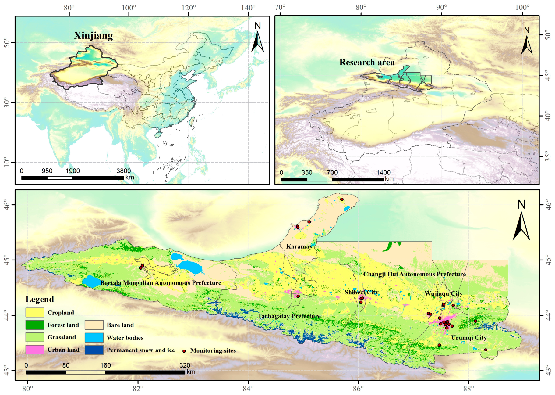
The TNSUA is located along the northern foothills of the Tianshan range, forming a 300 km-long, east–west-oriented belt of densely distributed cities, accounting for approximately 5.7% of the total area of Xinjiang. This region represents the most economically productive area in Xinjiang, with highly concentrated industrial and agricultural activities. It hosts about 83% of the region’s heavy industry and 62% of its light industry, and its gross domestic product has consistently contributed more than 40% of Xinjiang’s total [57,58]. However, this area also accounts for nearly half of the total coal consumption in Xinjiang. Due to low winter temperatures and a prolonged heating season, the intensive use of coal and other fossil fuels has led to severe air pollution. In recent years, with the adoption of air pollution mitigation measures, concentrations of particulate matter (PM₂.₅ and PM₁₀) have shown a declining trend, whereas O₃ concentrations have exhibited an increasing trend [57,59], drawing significant attention from policymakers and researchers. Therefore, this study selects 26 national air quality monitoring stations across seven prefectures and cities, ranging from Urumqi in the east to Bortala Mongolian Autonomous Prefecture in the west (Figure 1), to investigate the spatial distribution and source attribution of O₃.

Figure 1. Research areas and monitoring sites.

2.2. Data Sources

2.2.1. Surface O₃ Observations

The O₃ observational data used in this study were obtained from 26 monitoring stations (Figure 1) within the TNSUA, provided by the China National Environmental Monitoring Center (CNEMC) (https://www.cnemc.cn/). Data processing was conducted in accordance with the Ambient Air Quality Standards of China (GB 3095–2012), with preprocessing procedures following the approaches of Fan et al. (2020) [60] and Luo et al. (2023) [57]. Specifically, the quality-control procedures for the hourly O₃ observations consisted of three steps. First, hourly O₃ concentrations falling outside the physically reasonable atmospheric range were identified as invalid and removed. Second, consecutive records with identical values over extended periods were excluded to eliminate potential artifacts caused by instrument malfunction, communication interruption, or calibration failure. Third, daily average O₃ concentrations were calculated only when more than 20 valid hourly observations were available within a day; otherwise, the corresponding daily record was discarded. After quality control, including outlier screening and missing-value removal, approximately 3.35% of the total observations were excluded, indicating generally high data quality.

2.2.2. Ancillary Data for Surface O₃ Retrievals

Downward shortwave radiation (DSR) data play an important role in ozone formation, and the DSR data used in this study are derived from NASA’s Global Land Data Assimilation System (GLDAS). Meteorological factors also have significant impacts on ozone formation and transport. The meteorological datasets employed in this study are obtained from the ERA5-Land global reanalysis hourly data, including air temperature (TEM), evaporation (ET), total precipitation (TP), surface pressure (SP), relative humidity (RH), wind direction (WD, calculated from the u and v components of wind), and wind speed (WS). Satellite remote sensing data are also considered, as total column ozone is highly correlated with surface ozone. The Total Ozone Column (TotalO₃) data are sourced from the TROPOMI satellite, which provides daily observations with a spatial resolution of 3.5 km × 5 km. Digital Elevation Model (DEM) data are derived from the Shuttle Radar Topography Mission (SRTM) with a spatial resolution of 30 m × 30 m. Land use/land cover change (LUCC) and Normalized Difference Vegetation Index (NDVI) data are obtained from MODIS sensors, with a spatial resolution of 500 m × 500 m. The NDVI data have a temporal resolution of 16 days. In addition, human activity variables are included: population (POP) data are sourced from LandScan™, with a spatial resolution of 1 km, and nighttime light (NL) data are obtained from NPP-VIIRS at a spatial resolution of 500 m × 500 m. Detailed parameters of all datasets are provided in Table 1. All variables were resampled to a unified spatial resolution of 300 m using bilinear interpolation.

Table 1. Summary of data sources used in artificial intelligence algorithms.

Data	Variable	Description	Unit	Temporal Resolution	Spatial Resolution	Data Source
Ground measurements	O3	Ozone	μg·m−3	1 day	-	China National Environmental Monitoring Centre
Solar radiation	DSR	Downward shortwave radiation	W/m2	3 h	0.25° × 0.25°	GLDAS
Meteorological factors	TEM	2-m air temperature	°C	1 h	0.1° × 0.1°	ERA5-Land
	ET	Evaporation	mm	1 h	0.1° × 0.1°
	TP	Total precipitation	mm	1 h	0.1° × 0.1°
	SP	surface pressure	hPa	1 h	0.1° × 0.1°
	RH	Relative humidity	%	1 h	0.1° × 0.1°
	WD	Wind direction	°	1 h	0.1° × 0.1°
	WS	Wind speed	m/s	1 h	0.1° × 0.1°
Satellite remote sensing products	TotalO3	Total Ozone Column	mol/m2	1 day	3.5 km × 5 km	TROPOMI Satellite
	DEM	Digital elevation model	m	-	30 m × 30 m	SRTM
	LUCC	land use-cover change	-	1 year	500 m × 500 m	MODIS products
	NDVI	Normalized Difference Vegetation Index	-	16 day	500 m × 500 m
Human activity data	POP	Population	-	1 year	1 km × 1 km	LandScanTM
	NL	Night lighting	nW/cm2/sr	1 month	500 m × 500 m	NPP-VIIRS

2.2.3. Data for Spatial Source Analysis

The meteorological data used to drive the HYSPLIT backward trajectory model were obtained from the Global Data Assimilation System (GDAS) (https://ready.arl.noaa.gov/archives.php, accessed on 3 January 2025), provided by the National Centers for Environmental Prediction (NCEP), with a spatial resolution of 1° × 1°.

2.3. Methods

2.3.1. Spatial Inversion Model Development

Since O₃ is primarily generated through photochemical reactions, its formation is closely related to natural factors such as solar radiation and air temperature. Therefore, based on observed data from monitoring stations, artificial intelligence models are employed to learn the relationships between O₃ concentrations and natural variables (e.g., solar radiation, temperature, and precipitation). This process establishes a mapping between the explanatory variables and O₃ concentrations, forming an O₃ spatial inversion model. By applying the trained model to continuous spatial datasets of the explanatory variables, continuous spatial distributions of O₃ can be generated [61,62].

Feature Selection

To ensure the accuracy of the inversion model, features that exhibit significant correlations with O₃ (the dependent variable) were selected, while redundant, irrelevant, or highly collinear variables were removed. Pearson Correlation Analysis (Pearson), Spearman Rank Correlation Analysis (Spearman), Kendall Rank Correlation Coefficient (Kendall’s τ), and the Variance Inflation Factor (VIF) were employed for feature selection [63]. The corresponding calculation formulas are as follows:

$$r={\displaystyle \frac{{\sum }_{i=1}^n\left(x_i-\overline{x}\right)\left(y_i-\overline{y}\right)}{\sqrt{{{\sum }_{i=1}^n\left(x_i-\overline{x}\right)}^2}\sqrt{{{\sum }_{i=1}^n\left(y_i-\overline{y}\right)}^2}}}$$

(1)

$$\mathsf{\rho }=1-{\displaystyle \frac{6\sum d_i^2}{n\left(n^2-1\right)}}$$

(2)

$$\tau ={\displaystyle \frac{C-D}{\frac{1}{2}n\left(n-1\right)}}$$

(3)

$${VIF}_i={\displaystyle \frac{1}{1-R_i^2}}$$

(4)

Here, r denotes the Pearson correlation coefficient, ranging from −1 to 1. xᵢ represents the value of the feature variable for the i-th sample, and yᵢ represents the O₃ concentration for the i-th sample. $\overline{x}$ and ȳ denote the mean values of the feature variable and O₃ concentration, respectively, and n is the total number of samples. ρ denotes the Spearman rank correlation coefficient, ranging from −1 to 1, and dᵢ represents the difference in ranks between the feature variable and O₃ concentration for the i-th sample. τ represents Kendall’s rank correlation coefficient, with a range of −1 to 1, where C is the number of concordant pairs and D is the number of discordant pairs. VIFᵢ denotes the variance inflation factor for the i-th feature variable, and Rᵢ² represents the coefficient of determination obtained by regressing the i-th variable against all other variables.

Pearson, Spearman, and Kendall’s τ were employed to evaluate the relationships among candidate variables. Variables exhibiting excessively high correlations with other predictors were excluded to reduce redundancy. Subsequently, VIF was used to assess multicollinearity, and variables with VIF values greater than 10 were removed. The remaining variables, characterized by moderate inter-variable correlations and acceptable multicollinearity levels, were retained for model development.

Artificial Intelligence Model Selection

The relationship between O₃ formation and natural variables is highly nonlinear. ML and DL models are well suited to capture such complexity and nonlinearity, enabling the simulation of the multi-factor coupling mechanisms involved in O₃ photochemical formation and revealing the underlying relationships between explanatory variables and O₃ concentrations. Considering the characteristics of different ML models and their applications in the field of atmospheric environmental research, 16 representative models were selected for the retrieval of O₃ concentrations in the TNSUA. Based on the retrieval accuracy and computational efficiency of each model, the most suitable ML model for this study was identified. Detailed descriptions and applications of the 16 models are presented in Table 2.

Table 2. Artificial intelligence models selected in this study.

Model Types	Model Name	Abbreviation	Abbreviation	Reference
ML	Decision Tree	DT	Applied in research on air quality data.	[64]
	Random Forest	RF	Applied in research on CH4 and N2O emissions in China.	[65]
	Extremely Randomized Trees	ET	Extensively applied in research on complex non-linear environments.	[66]
	Adaptive Boosting	AdaBoost	Applied in research on the Air Quality Index (AQI) in major Indian cities.	[67]
	Gradient Boosting Decision Tree	GBDT	Applicable to the non-linear function fitting of large-scale, complex geographic environmental features.	[68]
	Extreme Gradient Boosting	XGBoost	Applied in high-precision near-surface PM2.5 concentration retrieval and spatial mapping in major South African cities.	[69]
	Light Gradient Boosting Machine	LightGBM	Applied in research on O3 concentrations in China.	[70]
	Categorical Boosting	CatBoost	Extensively applied in research on categorical feature processing.	[69]
	Support Vector Regression	SVR	Applied in research on urban air pollutants and localized meteorological features.	[69]
DL	Multilayer Perceptron	MLP	Applied in generalized modeling and non-linear feature extraction of complex environmental monitoring data.	[71]
	Deep Neural Network	DNN	Applied in localization research of atmospheric pollution sources.	[72]
	Deep Belief Network	DBN	Applicable to research on large-scale, high-dimensional environmental sequence data.	[73]
	Convolutional Neural Network	CNN	Applied in research on urban air quality.	[74]
	Long Short-Term Memory	LSTM	Applied in research on long-term time-series forecasting of atmospheric pollutants.	[75]
	Residual Neural Network	ResNet	Extensively applied in research such as high-level feature identification of spatial remote sensing imagery.	[76]
	Residual Network	ResNeXt	Applied in the prediction research of typhoon pathways and extreme meteorological trajectories.	[77]

Model Evaluation

Model validation plays a crucial role in ensuring the accuracy and robustness of the models. In this study, a 10-fold cross-validation approach was employed to evaluate and compare model performance. The dataset was randomly divided into 10 subsets, and an iterative training process was conducted in which 9 subsets were used for model training while the remaining subset was used for testing and validation. This rotating procedure ensures that all data are involved in the validation process. For model evaluation, three metrics were selected: the Coefficient of Determination (R²), Root Mean Squared Error (RMSE), and the Ratio of Performance to Deviation (RPD) [78,79,80]. The corresponding calculation formulas are as follows:

$$R^2=1-{\displaystyle \frac{{\sum }_{i=1}^n{\left(y_i-\widehat{y_i}\right)}^2}{{\sum }_{i=1}^n{\left(y_i-\overline{y_i}\right)}^2}}$$

(5)

$$RMSE=\sqrt{{\displaystyle \frac{1}{n}}{\sum }_{i=1}^n{\left(y_i-\widehat{y_i}\right)}^2}$$

(6)

$$RPD={\displaystyle \frac{SD}{RMSE}}={\displaystyle \frac{\sqrt{\frac{1}{n-1}{\sum }_{i=1}^n{\left(y_i-\widehat{y_i}\right)}^2}}{RMSE}}$$

(7)

Here, yᵢ represents the observed O₃ value for the i-th sample, ŷᵢ denotes the model-predicted O₃ value, and ȳ is the mean of all observed O₃ values. n is the total number of samples. SD represents the standard deviation of the observed O₃ concentrations, and RMSE is the root mean squared error between the predicted and observed values.

2.3.2. Shapley Additive Explanations

Based on the trained ML model, the SHAP method was applied to investigate the effects of 14 feature variables on near-surface O₃. Using the selected optimal model, SHAP was employed to perform interpretability analysis of the model outputs, thereby quantifying the contributions of individual feature variables to near-surface O₃. SHAP is an interpretable modeling framework based on game theory and local interpretability [81]. It quantifies the marginal contribution of each input variable by evaluating how the inclusion of that variable increases or decreases the model prediction for a given sample [82]. The corresponding calculation formula is as follows:

$${\phi }_i\left(f\right)=\sum _{S\subseteq N\backslash \left\{i\right\}}{\displaystyle \frac{\left|S\right|!\left(\left|N\right|-\left|S\right|-1\right)!}{\left|N\right|!}}\left[f(S\cup \{i\})-f\left(S\right)\right]$$

(8)

In the equation, φᵢ(f) represents the contribution of feature xᵢ (e.g., solar radiation) to near-surface O₃ (Y). S denotes a subset of features that excludes xᵢ, while N represents the set of all features. f(S) is the model prediction based on the feature subset S (without xᵢ), and f(S ∪ {xᵢ}) denotes the prediction after including xᵢ in the subset.

To facilitate the comparison of feature importance, the contribution percentage of each feature was calculated based on its mean absolute SHAP value. The contribution percentage was calculated as follows:

$$Mean\left(\left|{\phi }_i\right|\right)={\displaystyle \frac{1}{M}}{\displaystyle \sum _{j=1}^M}\left|{\phi }_i^{\left(j\right)}\right|$$

(9)

$$P_i={\displaystyle \frac{Mean\left(\left|{\phi }_i\right|\right)}{{\displaystyle {\sum }_{k=1}^N}Mean\left(\left|{\phi }_i\right|\right)}}\times 100\%$$

(10)

Here, ${\phi }_i^{\left(j\right)}$ denotes the SHAP value of feature i for the j-th sample, and M represents the total number of evaluation samples. P_i signifies the relative contribution percentage of feature i, N is the total number of feature variables (N = 14), and $Mean\left(\left|{\phi }_i\right|\right)$ represents the global feature importance score.

2.3.3. Spatial Source Analysis Method

Backward Trajectory Analysis

To investigate the spatial origins of O₃, the Hybrid Single-Particle Lagrangian Integrated Trajectory (HYSPLIT) model was employed in combination with the GDAS dataset to perform 72-h backward trajectory simulations at an arrival height of 500 m above ground level, aiming to identify potential transport pathways of air masses reaching the study area. The MeteoInfo software (Version 3.8.7) was used for trajectory simulation and analysis, and the TrajStat plugin within MeteoInfo was applied to conduct statistical analysis and visualization of the HYSPLIT-generated trajectories [28,30,83].

Potential Source Contribution Function (PSCF) Analysis

The PSCF method was employed to identify potential pollution source regions in the study area. The calculation formula is presented in Equation (9).

$${PSCF}_{ij}={\displaystyle \frac{m_{ij}}{n_{ij}}}$$

(11)

In the equation, PSCF_(ij) represents the ratio of the number of trajectory endpoints mᵢⱼ exceeding a specified threshold to the total number of trajectory endpoints nᵢⱼ within grid cell i,j. To reduce the influence of small nᵢⱼ values in some grid cells, a weighting function Wᵢⱼ is applied to the PSCF values. The determination of this weighting function follows the approaches of Fan et al. (2019) [84] and Zhang et al. (2023) [46], with the calculation formulas provided in Equations (10) and (11), where Nₐᵥₑ represents the average nᵢⱼ across all grid cells.

$${\mathit{WPSCF}}_{\mathit{ij}}={\mathit{PSCF}}_{\mathit{ij}}\times {\mathrm{W}}_{\mathit{ij}}$$

(12)

$$W_{\mathit{ij}}=\{\begin{array}{c}1.00, n_{\mathit{ij}}>3n_{\mathit{a}\mathit{v}\mathit{e}}\\ 0.70, 3n_{\mathit{a}\mathit{v}\mathit{e}}\ge n_{\mathit{ij}}>1.5n_{\mathit{a}\mathit{v}\mathit{e}}\\ 0.40, 1.5n_{\mathit{a}\mathit{v}\mathit{e}}\ge n_{\mathit{ij}}>n_{\mathit{a}\mathit{v}\mathit{e}}\\ 0.17, n_{\mathit{a}\mathit{v}\mathit{e}}\ge n_{\mathit{ij}}\end{array}$$

(13)

Concentration-Weighted Trajectory (CWT) Analysis

Although the PSCF method can, to some extent, identify the probability of pollution occurrence in different regions and thereby infer potential source areas, its results are strongly dependent on the selected threshold and cannot effectively reflect the severity of pollution when concentrations exceed that threshold. In contrast, the CWT method calculates concentration-weighted trajectories, which can better represent the intensity of pollution. Therefore, the CWT approach was employed to quantify the relative contributions of different potential source regions [31,32]. The corresponding calculation formulas are provided in Equations (12) and (13).

$${\mathit{CWT}}_{\mathit{ij}}={\displaystyle \frac{1}{{\sum }_{l=1}^M{\tau }_{\mathit{ijl}}}}{\displaystyle \sum _{l=1}^M}{C}_l{\tau }_{\mathit{ijl}}$$

(14)

$${\mathit{WCWT}}_{\mathit{ij}}={\mathit{CWT}}_{\mathit{ij}}\times W_{\mathit{ij}}$$

(15)

In the equation, CWT_(ij) represents the average weighted concentration in grid cell i,j. M denotes the total number of trajectories, τᵢⱼˡ is the residence time of trajectory l within grid cell i,j, and Cˡ represents the pollutant concentration associated with trajectory l when passing through grid cell i,j.

3. Results

3.1. Analysis of Spatial Distribution Results

3.1.1. Correlation Analysis of Characteristic Variables

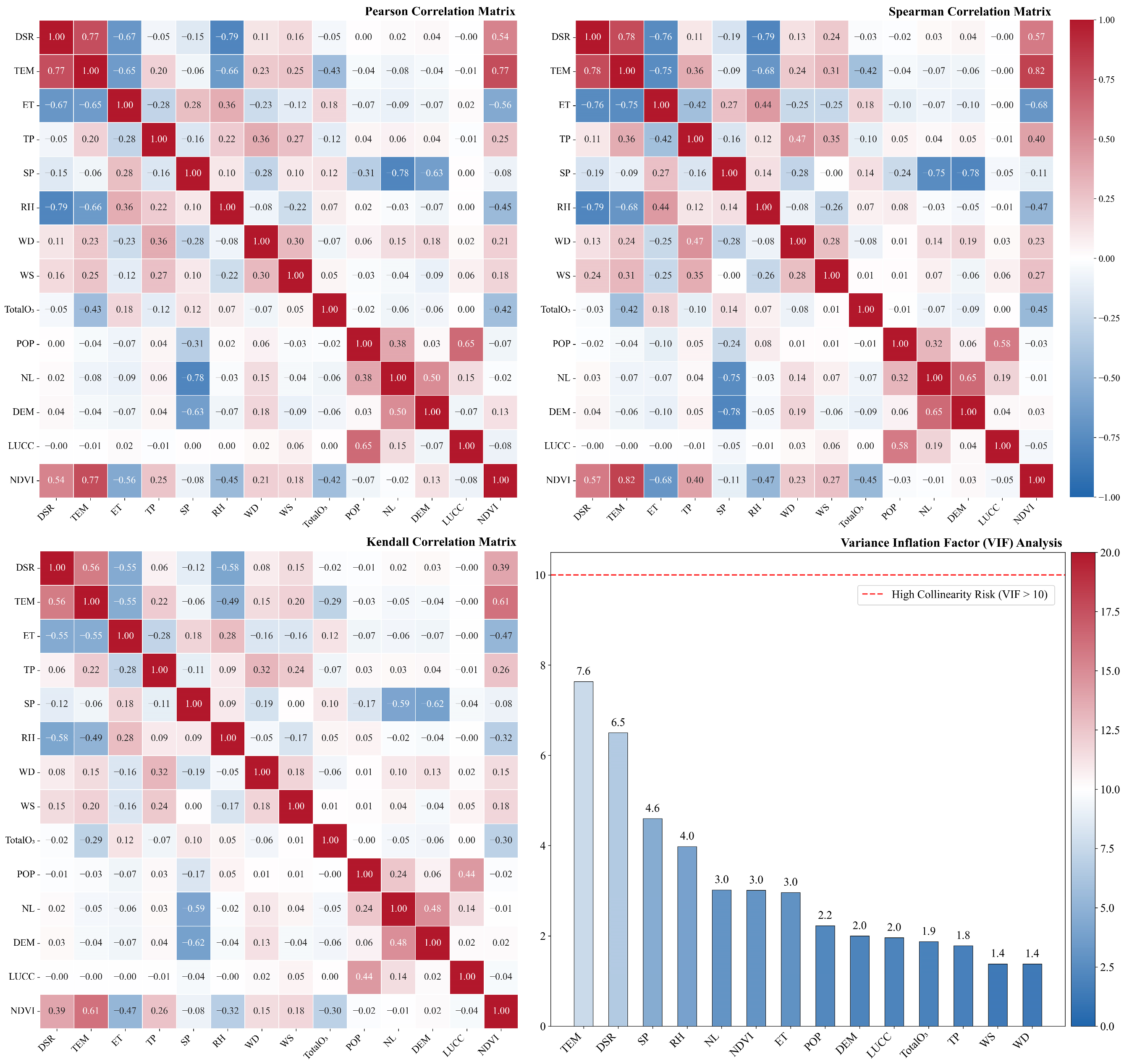
The correlations and collinearity among the feature variables were analyzed. Pearson was used to assess linear relationships between variables, while Spearman and Kendall’s τ were applied to evaluate nonlinear relationships. The VIF was used to assess collinearity among the features. As shown in Figure 2, the results of the Pearson, Spearman, and Kendall’s τ analyses indicate generally weak correlations among the feature variables, with no excessively high correlation coefficients observed. With respect to collinearity, all feature variables exhibited VIF values below 10, suggesting the absence of significant multicollinearity among the predictors.

Figure 2. Correlation and collinearity analysis figure.

3.1.2. Model Comparison and Validation

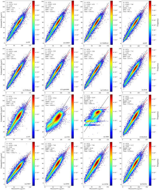
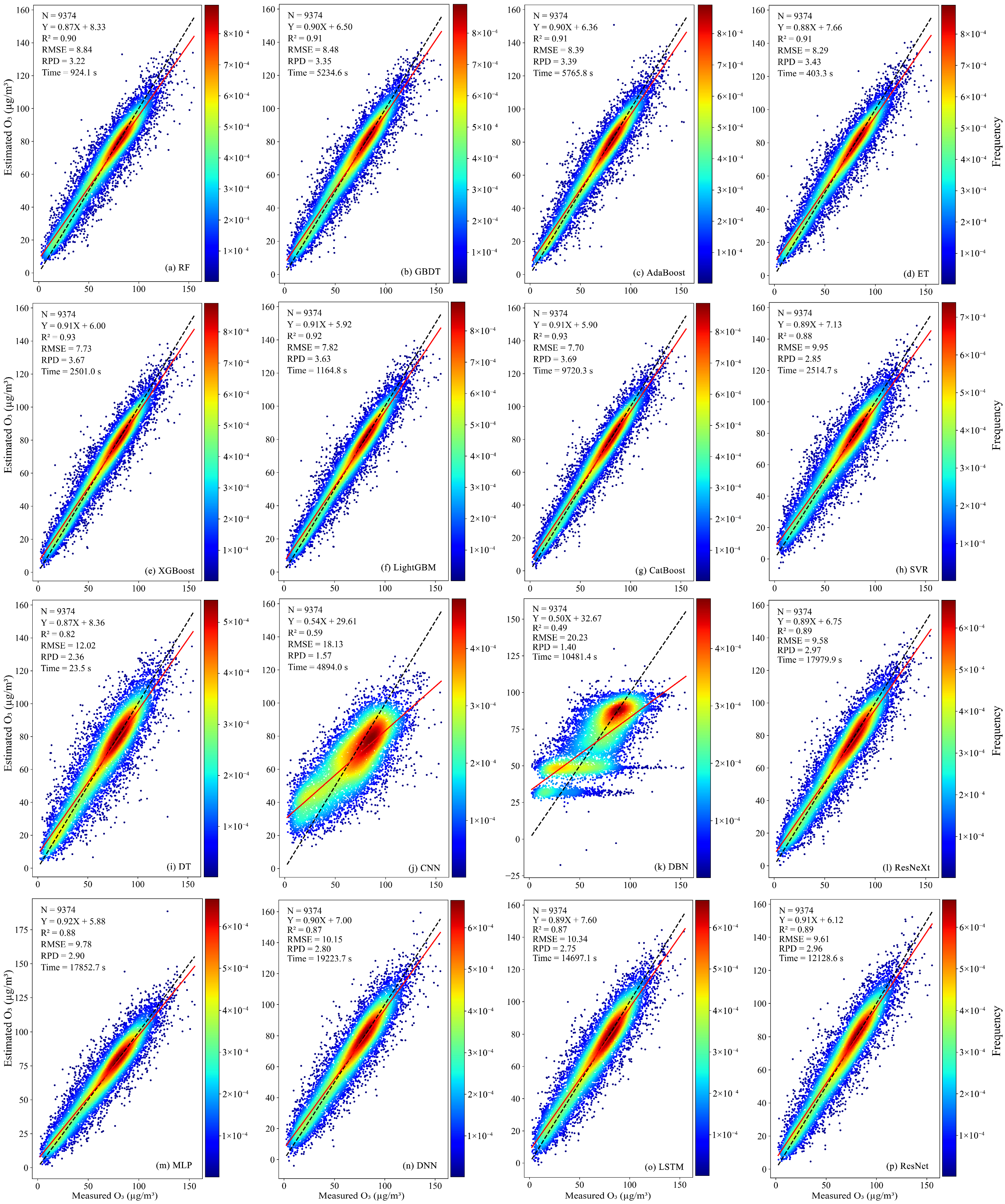
Figure 3 compares the performance and efficiency of 16 artificial intelligence models in estimating O₃ concentrations across the TNSUA. All models were trained on the same dataset (sample size N = 9374) with hyperparameters optimized using Bayesian tuning. The best-performing models were XGBoost and CatBoost, both achieving R² values of 0.93 and RPD values above 3. Among them, XGBoost was faster, with a runtime of 2501.0 s. Models with R² values between 0.90 and 0.92 included LightGBM, RF, GBDT, AdaBoost, and ET, which also performed well. ET was the most efficient among these, with a runtime of 403.3 s. Models with R² values between 0.80 and 0.90 included SVR, DT, ResNeXt, MLP, DNN, LSTM, and ResNet, showing relatively lower performance, with RPD values below 3. The DL models in this group had particularly long runtimes, with the DNN model taking 19,223.7 s—the longest among all models. The poorest-performing models were CNN and DBN, with R² values of 0.59 and 0.49, respectively, indicating limited capability for estimating O₃ concentrations in this region. Moreover, DBN had a runtime of 10,481.4 s, reflecting relatively low efficiency. Considering both performance and computational efficiency, XGBoost was selected as the optimal model for estimating O₃ concentrations in the TNSUA, enabling high-resolution mapping of O₃ spatial distribution in the study area.

Figure 3. Model evaluation figure. The red solid line indicates the fitted regression line, and the black dashed line represents the 1:1 reference line.

3.1.3. Inversion Based on Excellent Inversion Model

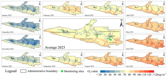
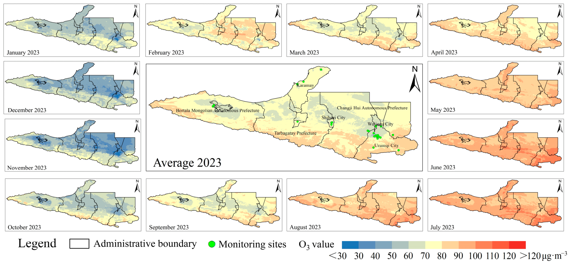
Figure 4 presents the spatial distribution of O₃ concentrations estimated by the XGBoost model. According to the inversion results, the high-concentration areas of O₃ in the TNSUA are primarily located in the southern part of Urumqi, the southern part of Changji Prefecture, and the southern part of Tacheng. The reason for this phenomenon is that the southern part of Urumqi City, the southern part of Changji Prefecture, and the southern part of Tacheng Prefecture are located in the northern piedmont zone of the Tianshan Mountains. This region possesses high vegetation coverage that emits biogenic volatile organic compounds (BVOCs); moreover, because this area is situated at the southern edge of the cities, the pollutant emissions are also relatively high, thereby generating O₃ via photochemical reactions. Moreover, the high-concentration area in southern Urumqi exhibits the highest O₃ levels and the widest spatial extent. In June, the maximum O₃ concentration in southern Urumqi exceeds 120 μg·m⁻³, while the high-value areas in southern Changji and southern Tacheng are mainly in the range of 100–110 μg·m⁻³ during summer. The spatial inversion results also indicate a seasonal pattern of O₃, with higher concentrations in summer and lower in winter. The locations of high-value areas remain generally consistent across different months, showing that southern Urumqi, southern Changji, and southern Tacheng consistently have higher concentrations relative to other regions throughout the year. This pattern is attributed to the complex interplay of multiple factors. O₃ concentrations are influenced by atmospheric processes and photochemical reactions. Higher temperatures in summer promote O₃ formation, leading to generally elevated concentrations in these regions. Vegetation also contributes by emitting BVOCs, which participate in photochemical reactions to generate O₃. The higher vegetation cover in southern Urumqi, southern Changji, and southern Tacheng further contributes to these areas being high-concentration zones for O₃.

Figure 4. XGBoost-derived O₃ concentration inversion results.

3.1.4. Spatio-Temporal Feature Analysis

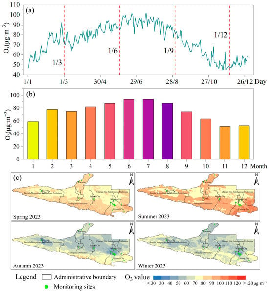
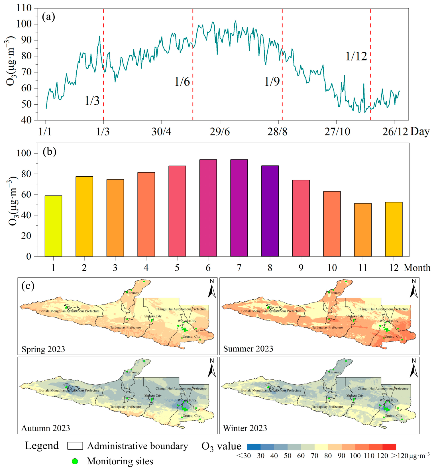
Figure 5 illustrates the spatiotemporal characteristics of O₃. On a daily scale, near-surface O₃ in the TNSUA in 2023 exhibited higher concentrations in summer and lower concentrations in winter, with spring concentrations generally exceeding those in autumn. On a monthly scale, the months with the highest average O₃ concentrations were June (93.98 μg·m⁻³) and July (93.92 μg·m⁻³), while the lowest monthly average occurred in November (51.50 μg·m⁻³). Regarding seasonal spatial distribution, the high-concentration areas remained largely consistent across the four seasons, generally showing higher values around the periphery and lower values in the central region, with high-concentration zones primarily located in the southern part of the study area. The seasonal distribution also reflected that spring average concentrations exceeded those in autumn, with spring high-concentration areas more widely distributed. In summer, the high-concentration areas were most extensive. Regions with average O₃ concentrations of 90–100 μg·m⁻³ were mainly located in southern Urumqi, southern Changji, southern Tacheng, southern Bozhou, and Karamay. Notably, the high-concentration area in southern Urumqi reached the highest average O₃ levels, exceeding 110 μg·m⁻³, marking it as a critical area for O₃ control in the TNSUA.

Figure 5. Spatiotemporal Characteristics Analysis Figure ((a): Daily mean variation in O₃, (b): Monthly mean variation in O₃, (c): Seasonal mean spatial distribution of O₃).

3.2. Analysis of Influencing Factors

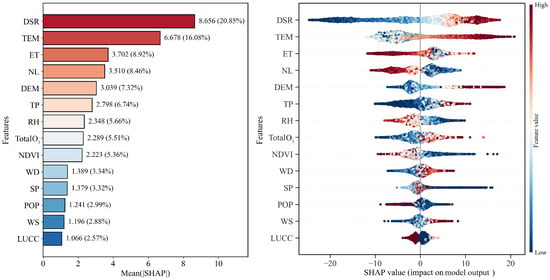
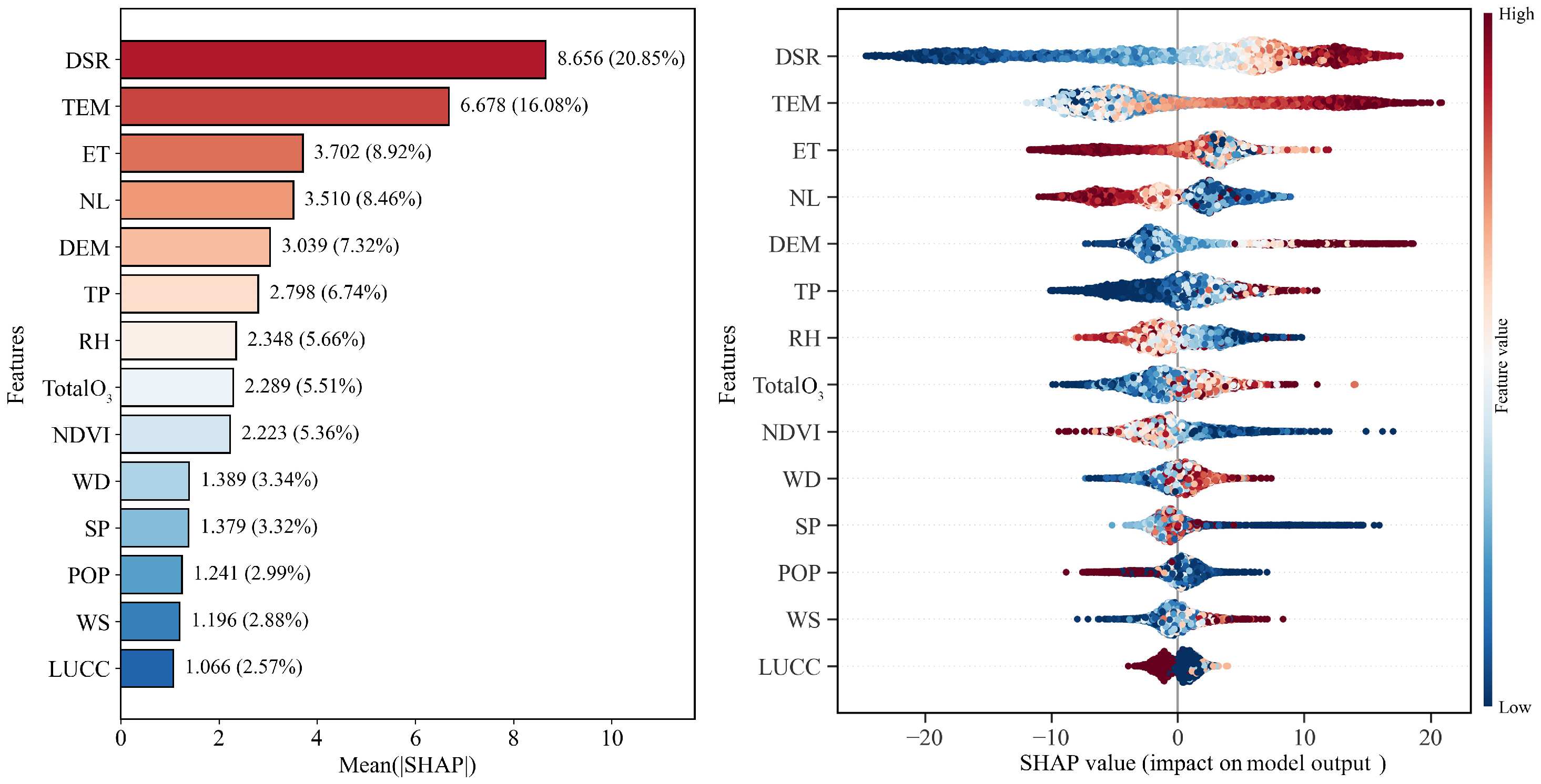
Based on the continuous spatial distribution of near-surface O₃ derived from feature variables and the trained feature relationships, the key driving factors influencing near-surface O₃ were investigated. Using the XGBoost model combined with the SHAP algorithm, environmental variables with significant contributions to near-surface O₃ were identified. The analysis results (Figure 6) indicate that DSR and TEM are the primary drivers of near-surface O₃ in the TNSUA. DSR has the highest mean absolute SHAP value of 8.656 (20.85%), followed by TEM with a mean absolute SHAP value of 6.678 (16.08%). According to the SHAP value distributions, both DSR and TEM exhibit a strong positive correlation with O₃ concentrations (high-concentration areas correspond to positive SHAP values), which is consistent with photochemical reaction mechanisms, where strong solar radiation and high temperatures accelerate the conversion of precursors. In contrast, WS and LUCC contributed less, with mean absolute SHAP values of 1.196 (2.88%) and 1.066 (2.57%), respectively. Their SHAP values are highly concentrated around zero, indicating that in 2023, the variability of WS and the spatial heterogeneity of LUCC had a relatively limited influence on O₃ concentrations compared with strong meteorological fluctuations such as DSR and TEM. This suggests that O₃ pollution in the region is more controlled by large-scale meteorological conditions and regional emissions rather than local microclimate or surface cover adjustments.

Figure 6. Feature importance and SHAP contribution analysis figure.

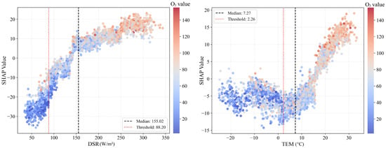
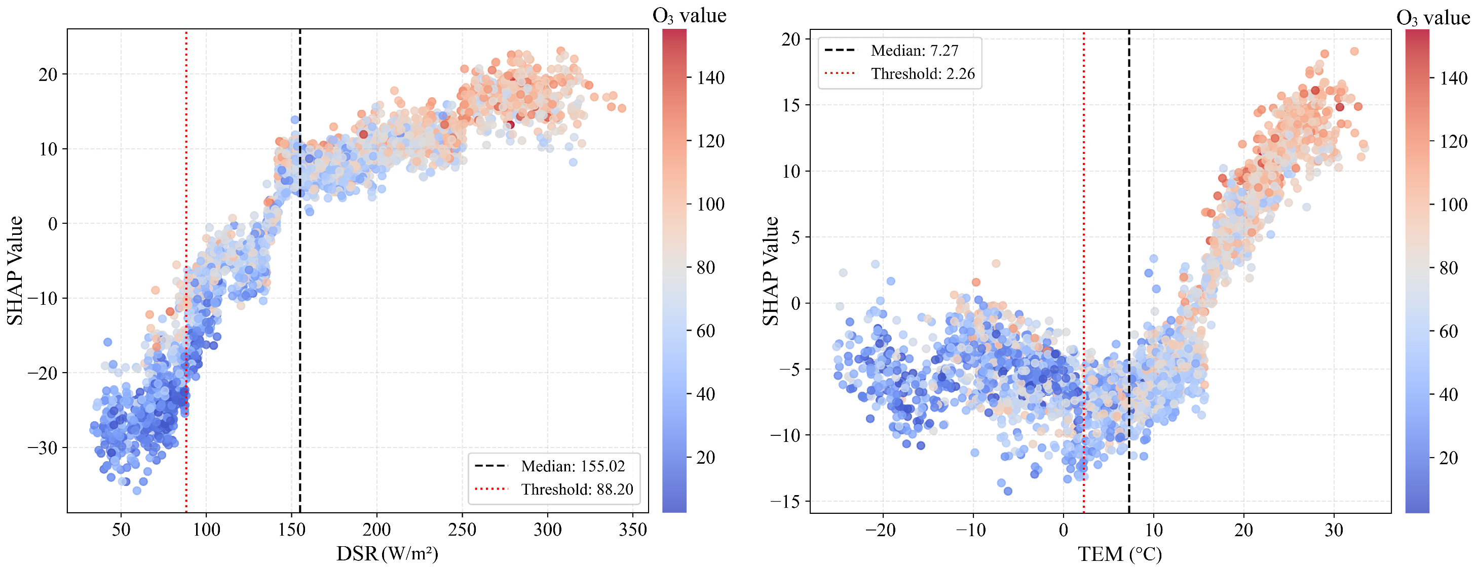
Based on the feature contribution analysis, feature dependence plots were generated for the most influential variables (DSR and TEM) to further investigate their threshold effects (Figure 7). Downward shortwave radiation (DSR) exhibits a significant positive contribution to near-surface O₃ concentrations. When DSR is below the threshold of 88.20 W/m², SHAP values are negative, indicating that low radiation conditions strongly inhibit O₃ formation. As DSR increases, SHAP values rise, and once it exceeds the median value of 155.02 W/m², the positive contribution sharply strengthens, highlighting DSR as a key driver of photochemical reactions. Air temperature shows a clear positive correlation with near-surface O₃ concentrations. When TEM is below 2.26 °C, SHAP values are mostly negative. As the temperature rises above 10 °C, the slope of the curve increases significantly, reflecting the strong influence of high temperatures on O₃ concentrations. This effect is likely due to the acceleration of photochemical reaction rates at higher temperatures and increased BVOC emissions from vegetation, which synergistically promote O₃ formation. Moreover, when examining the combined feature dependence plots, high-concentration samples (dark red) are concentrated in the high-value ranges of DSR and TEM (upper-right corner), where the SHAP positive contributions are maximal. This strong consistency indicates that the model accurately captures the driving mechanisms of high radiation and high temperature on near-surface O₃. The formation of near-surface O₃ in the TNSUA is strongly regulated by meteorological thresholds. For precise atmospheric management, periods when DSR and TEM exceed the thresholds (e.g., DSR > 88.20 W/m² and TEM > 2.26 °C) should be prioritized for control measures.

Figure 7. Dependence plots of key features.

3.3. Spatial Source Analysis

Based on the spatial distribution results of O₃, high concentrations in the TNSUA are mainly concentrated in southern Urumqi, southern Changji Prefecture, and southern Tacheng, with the highest O₃ levels observed in southern Urumqi. Therefore, the high-concentration area in southern Urumqi was selected for backward trajectory clustering analysis, potential source analysis, and CWT analysis, in order to investigate the sources and transport pathways of O₃ from a spatial perspective.

3.3.1. Results of Backward Trajectory Analysis

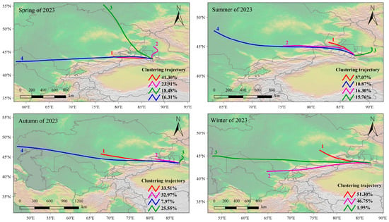
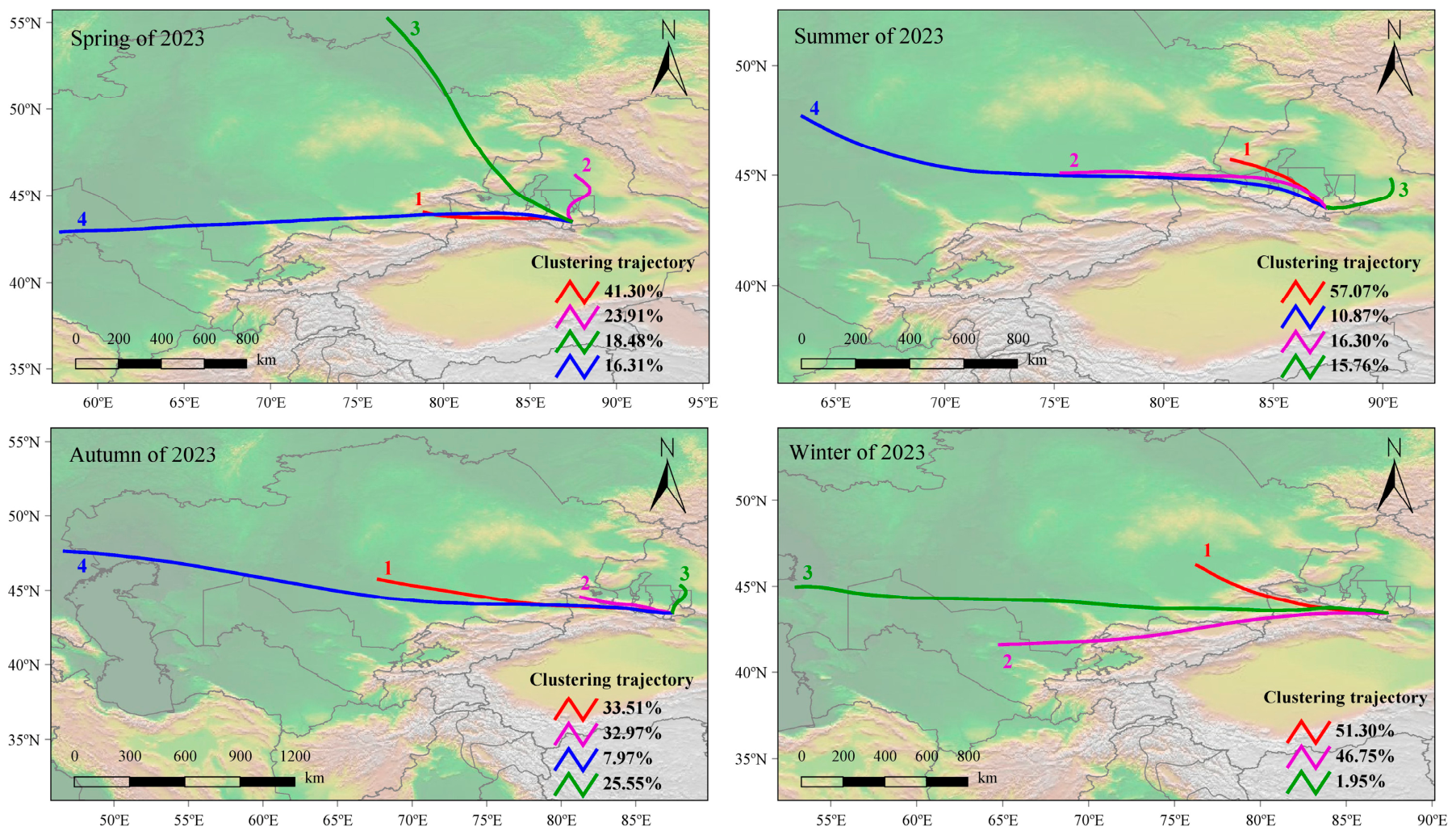
Figure 8 presents the clustering results of backward air mass trajectories for southern Urumqi. In spring, Cluster 1 (accounting for 41.30%) represents the dominant airflow trajectory affecting southern Urumqi, originating from eastern Kazakhstan and traveling eastward through the Ili River Valley before reaching the study area. In summer, the primary airflow trajectory (Cluster 1, accounting for 57.07%) originates from the northwest of the TNSUA, moving from northwest to southeast toward southern Urumqi. In both autumn and winter, the dominant airflow trajectories originate from Kazakhstan and move eastward to southern Urumqi. Overall, the backward trajectory analysis across all four seasons indicates that the main airflows influencing southern Urumqi predominantly originate from the west, traveling eastward along the northern and southern foothills of the Tianshan Mountains before reaching the study area.

Figure 8. Backward trajectory clustering map for southern Urumqi.

3.3.2. Potential Source Analysis

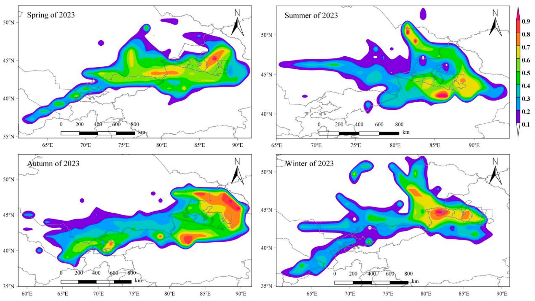
Since backward trajectory clustering analysis can only identify the directional influence of air masses on pollutant transport and cannot quantify the contributions of potential source regions, the PSCF method was employed to analyze the likely source areas. The results are presented in Figure 9, where high WPSCF values indicate the presence of potential source regions. The analysis shows that in spring, the potential source regions for O₃ in southern Urumqi are mainly located in the northeastern part of the TNSUA (WPSCF > 0.9) and the Ili River Valley region (WPSCF > 0.7). In summer, the potential sources are primarily distributed around the TNSUA and eastern Kazakhstan (WPSCF > 0.9). In autumn, the potential sources are primarily located in the northeastern and southwestern edges of the urban agglomeration. In winter, the potential sources are mainly concentrated in the western and central parts of the study area. Considering all four seasons, the potential source regions of O₃ affecting southern Urumqi are generally concentrated in the surrounding areas of the TNSUA, eastern Kazakhstan, and northern Kyrgyzstan.

Figure 9. Seasonal PSCF distribution maps of O₃ for southern Urumqi.

3.3.3. Concentration Weight Trajectory Analysis

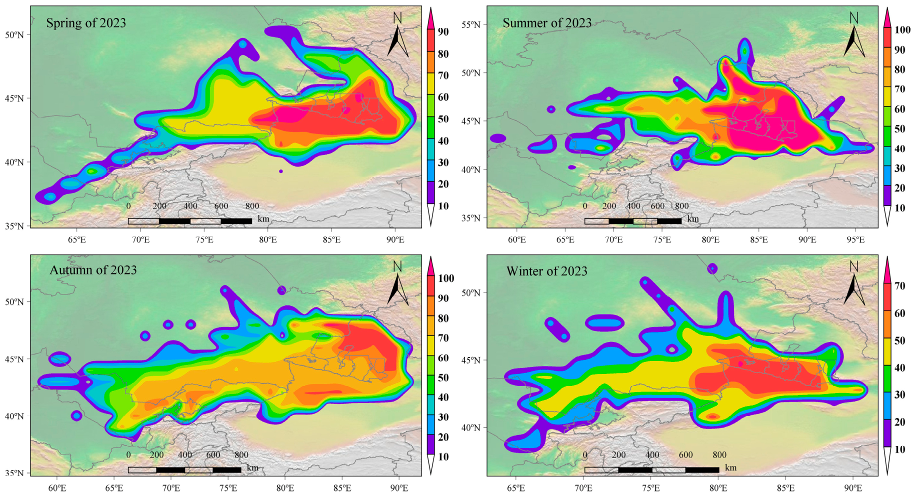
Although the PSCF method can analyze the contribution of potential source regions, it is constrained by threshold values and cannot assess the severity of pollution when concentrations exceed the threshold. Therefore, the CWT method was used to quantitatively reflect pollution intensity, and the results are presented in Figure 10. The analysis indicates that in spring, the high WCWT regions for O₃ in southern Urumqi are mainly distributed around the TNSUA, with the Ili River Valley in the southwest showing WCWT values greater than 90 μg·m⁻³. In summer, both the urban agglomeration and its surrounding areas are high WCWT regions for O₃ (WCWT > 100 μg·m⁻³), and eastern Kazakhstan also exhibits high WCWT values (>90 μg·m⁻³). In autumn, the high WCWT regions for O₃ are primarily located to the northeast and south of the study area, as well as near the border between Kazakhstan and Kyrgyzstan. In winter, the high WCWT regions are mainly concentrated around the TNSUA and its southern areas (WCWT > 60 μg·m⁻³), with generally lower WCWT values, reflecting the low O₃ concentrations typical of the winter season.

Figure 10. Seasonal CWT distribution maps of O₃ for southern Urumqi.

4. Discussion

4.1. Model Applicability and Analysis of Differences in Spatial Inversion

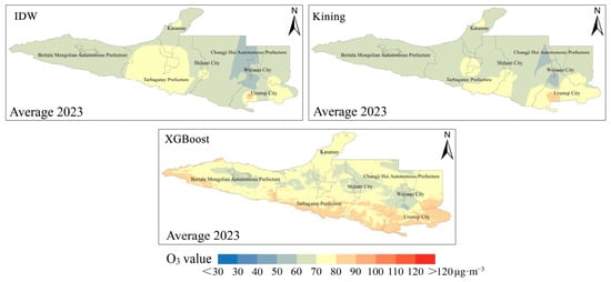
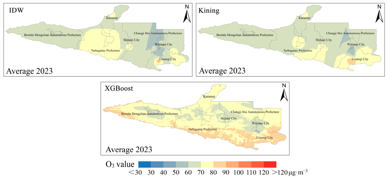
This study employed 16 artificial intelligence models and selected the optimal model to investigate the spatial distribution of O₃ in the TNSUA. The results were compared and discussed with previous studies focusing on near-surface O₃ distribution. Earlier studies have visualized spatial distributions based on monitoring station data [85,86], which can only provide a general characterization of spatial patterns but cannot produce continuous spatial fields. Other studies have applied classical geostatistical interpolation methods [87], such as Inverse Distance Weighted interpolation (IDW) and Kriging interpolation (Kriging). Although these methods generate continuous spatial surfaces, they are constrained by predefined mathematical formulations, resulting in limited spatial continuity [35,88]. In this study, both IDW and Kriging methods were applied to the study area and compared with artificial intelligence-based approaches, as shown in Figure 11. The interpolation results exhibit relatively poor continuity and are strongly influenced by station distribution and model assumptions. The interpolation results exhibit relatively poor continuity, whereas the XGBoost model shows much better spatial continuity. The fundamental reason for this difference lies in the distinct underlying mechanisms of the two types of approaches. Traditional interpolation methods, such as IDW and Kriging, estimate O₃ concentrations mainly based on the spatial relationships among monitoring stations. In essence, these methods follow the ‘First Law of Geography’ and calculate O₃ concentrations according to spatial proximity. Therefore, their outputs are highly dependent on the distribution of monitoring stations and are prone to local over-smoothing effects, resulting in relatively poor continuity [89,90,91]. In contrast, the XGBoost model establishes nonlinear relationships between surface O₃ concentrations and 14 environmental variables (e.g., DSR, TEM, and NDVI), thereby overcoming the limitations of purely geometric interpolation and enabling the capture of complex nonlinear interactions associated with O₃ formation. Furthermore, conventional interpolation approaches are unable to characterize complex terrain effects and spatial heterogeneity, whereas the XGBoost model can learn the relationships between O₃ and variables such as DEM and LUCC, thereby identifying local spatial heterogeneity. In addition, O₃ concentrations are influenced by photochemical reactions and atmospheric transport processes, and their spatial distributions often deviate from the assumptions required by traditional interpolation methods. Therefore, artificial intelligence algorithms such as XGBoost are better able to capture spatial heterogeneity, leading to more spatially continuous results than those obtained using conventional interpolation methods. In studies using artificial intelligence for surface O₃ mapping, most previous research has relied on only one to three ML models [92,93], whereas this study systematically compared 16 models and identified the optimal one. The results indicate that the XGBoost model exhibited excellent performance (R² = 0.93, RPD > 3), which may be closely related to the unique meteorological and pollution characteristics of the TNSUA, a typical arid region. In this arid area, the photochemical processes of surface O₃ are influenced by extreme environmental conditions, including strong solar radiation and persistently high temperatures during summer, resulting in highly complex environmental conditions. Owing to its gradient boosting tree framework, XGBoost can effectively model the complex nonlinear relationships among high-dimensional environmental variables [94], while reducing bias and the risk of overfitting through iterative optimization. Therefore, it is more suitable for the spatial inversion of O₃ under the complex environmental conditions of arid regions. Compared with ensemble learning models such as RF and ET, XGBoost employs sequential tree building and gradient boosting, enabling it to more effectively identify complex interactions among environmental factors and thereby improve model generalization ability [95]. Although SVR and some DL models have advantages in handling complex pattern recognition tasks, their performance did not reach the optimal level due to limitations associated with sample size, characteristics of regional environmental variables, and model parameter sensitivity [96]. In particular, in regional air quality inversion studies with relatively limited sample sizes, DL models may fail to fully exploit their advantages because of their high parameter complexity [97]. Therefore, the superior performance of XGBoost in this study may fundamentally stem from its stable capability to model complex nonlinear relationships under limited sample conditions, as well as its strong adaptability to heterogeneous environmental variables from multiple sources. Furthermore, compared with previous studies focusing on large-scale regional O₃ distribution using artificial intelligence models [61,62], this study focuses on an urban agglomeration scale and achieves high-resolution mapping of near-surface O₃. This provides a more refined representation of spatial patterns and offers important references for air pollution prevention and control in urban agglomerations.

Figure 11. Comparison of interpolation results and artificial intelligence model results.

4.2. Discussion of Influencing Factors

Based on the optimal model, this study applied the SHAP algorithm to quantify the contributions of environmental variables to near-surface O₃ concentrations. During the training of the spatial distribution model, the nonlinear influence mechanisms of environmental variables on near-surface O₃ were systematically analyzed. The results indicate that meteorological factors—particularly DSR and TEM—are the dominant drivers of near-surface O₃ in the TNSUA, which is highly consistent with the physicochemical mechanisms of O₃ formation. Gagliardi et al. (2025) [98], in their study of the Basilicata Region (Southern Italy), also found that meteorological variables played a dominant role in O₃ variability throughout the study period, consistent with the findings of this study. However, their key variables included relative humidity, wind speed, and temperature, which differs from our results. In this study, relative humidity and wind speed were found to have relatively weak effects on O₃ in the study region, with solar radiation and temperature emerging as the primary drivers. This discrepancy may be attributed to regional differences: the study area of Gagliardi et al. (2025) [98] is a coastal region, where meteorological factors such as humidity have stronger influences, whereas the present study area is an inland region, where O₃ formation is more strongly controlled by large-scale meteorological conditions such as solar radiation and temperature. The identification of DSR and TEM as key drivers is consistent with previous studies investigating near-surface O₃ across China [61,62]. Furthermore, by analyzing threshold effects, this study provides deeper insights into the specific roles of DSR and TEM. The study area is a typical arid urban agglomeration. When the region exceeds the thresholds of solar radiation and temperature (i.e., DSR > 88.20 W/m², TEM > 2.26 °C), the positive effects of DSR and TEM on O₃ concentrations become more pronounced, leading to elevated O₃ levels. The solar radiation threshold of 88.20 W/m² may be associated with relatively weak solar radiation conditions, such as those occurring in the early morning or early spring. When radiation is below this threshold, the low solar irradiance limits photochemical reactions involved in O₃ formation. In contrast, when radiation exceeds this threshold, photochemical reactions are enhanced, thereby promoting O₃ production [52,99]. The temperature threshold of 2.26 °C may correspond to relatively low temperatures in early spring. When temperature exceeds this threshold, it may be associated with increased emissions of BVOCs from vegetation, and the increase in temperature further enhances the photochemical reactions involved in O₃ formation [100,101]. The identified thresholds offer valuable references for precise air pollution control in the region, suggesting that emissions should be strictly regulated during periods when these thresholds are exceeded to mitigate potential O₃ pollution peaks.

4.3. Analysis of Spatial Sources

This study conducted source analysis specifically on the high-value areas identified in the spatial distribution of O₃, enabling precise identification of the most severely polluted regions and thereby deriving conclusions about their spatial sources. Compared with prior studies—such as Guan et al. (2019) [28], where the authors used city centers as reference points, and Yin et al. (2021) [32], where the authors used monitoring stations for source tracing—this study integrates the spatial distribution results of O₃ to accurately pinpoint the exact latitude and longitude of high-concentration areas, making the spatial source analysis more precise. This provides a basis for targeted pollution control in high-value areas, aligning source analysis results with practical pollution management needs. The analysis indicates that the primary transport pathway for O₃ in southern Urumqi originates from western airflows, traveling along the northern and southern slopes of the Tianshan Mountains to the high-concentration areas. Similarly, Zhang et al. (2023) [46], in their study on aerosol sources in Urumqi, found that the aerosol optical depth (AOD) source trajectories were mainly distributed along the western slope of the Tianshan Mountains. This pattern may be attributed to the influence of the North Atlantic warm current on Xinjiang, with moisture primarily transported via western airflows [102], highlighting the significant role of western airflows in the spatial transport of O₃.

4.4. Control Strategies and Recommendations

Based on the identified spatial distribution characteristics, key driving factors, and pollution source transport pathways, the following targeted control strategies and recommendations are proposed to address the O₃ pollution problem in the TNSUA. First, in terms of spatial management, key prevention and control efforts should focus on the southern parts of Urumqi, Changji Prefecture, and the Tacheng region, allowing for the formulation of a joint prevention and control policy across these three areas. Second, since DSR and TEM are the critical driving factors influencing near-surface O₃ in this urban agglomeration, targeted regulations should be deployed against these two influencing factors; especially during the summer period, temporary emission reduction measures for O₃ precursors should be strengthened to prevent the occurrence of heavy pollution events. Third, given that western airflows constitute the primary transport pathway affecting O₃ pollution within the study region, collaborative management of potential pollution source emissions from the western direction should be tightened, while regional cooperation and information sharing with western territories should be enhanced to mitigate the impacts of spatial transport on localized O₃ pollution. Finally, as meteorological factors exert a profound influence on O₃ generation in arid urban clusters, integrating meteorological forecasting with O₃ pollution early-warning systems could substantially upgrade pollutant prevention and control. These measures may provide a scientific reference for precise O₃ pollution control, regional coordinated management, and the formulation of air quality policies in arid urban agglomerations.

4.5. Limitations and Outlook

This study, based on high-precision observational data and multi-source environmental variables, developed a near-surface O₃ spatial inversion model suitable for arid urban clusters, achieving high-accuracy daily spatial reconstruction of O₃ over the TNSUA. Using SHAP analysis, the study quantified the regulatory effects of key meteorological factors on O₃ formation, while combining HYSPLIT backward trajectories and PSCF/CWT methods to precisely identify transport pathways and potential source regions of high-concentration areas, providing scientific support for air quality monitoring and cross-regional coordinated emission reduction in urban clusters. However, certain limitations exist: the study relied solely on data from 2023, lacking multi-year long-term monitoring, which may limit capturing long-term O₃ trends; moreover, the spatial inversion model does not fully account for complex chemical reactions and dynamic local emissions, and the potential source analysis has limited resolution in assessing local transport and terrain effects. In addition, while backward trajectory analysis combined with PSCF/WCWT methods can effectively identify potential source regions of ozone, the trajectory calculation is affected by the resolution of meteorological data (GDAS 1° × 1°), and this method mainly focuses on horizontal transport paths, without considering the influence of vertical transport processes on ozone transport. Future work could incorporate multi-year continuous observations and high-resolution emission inventories, combined with atmospheric chemistry models, to further improve the precision of O₃ formation mechanism analysis and extend the approach to a wider range of arid urban clusters, providing scientific guidance for precise air pollution control, regional coordinated management, and policy development.

5. Conclusions

(1)

After comparing 16 artificial intelligence models, including DT, RF, ET, GBDT, CatBoost, XGBoost, and LightGBM, the XGBoost model showed the best performance for O₃ inversion in the TNSUA, with an R² of 0.93 and an RPD of 3.67, while also demonstrating relatively high computational efficiency. The second-best model was CatBoost, which also had an R² of 0.93, but its computational efficiency was lower. Based on the XGBoost inversion results, the high-value areas of O₃ concentration in the TNSUA are mainly concentrated in southern Urumqi, southern Changji Prefecture, and southern Tacheng region, with southern Urumqi exhibiting the highest concentrations and the most extensive high-value area, reaching a summer maximum exceeding 110 μg·m⁻³.

(2)

By analyzing the contributions of the feature variables, DSR and TEM were identified as the key drivers influencing near-surface O₃ in the TNSUA. The SHAP value of DSR was 8.656 (accounting for 20.85% of the contribution), and TEM had a SHAP value of 6.678 (16.08% contribution). The threshold and median values of DSR affecting O₃ in the study area were 88.20 W/m² and 155.02 W/m², respectively, while TEM thresholds and median values were 2.26 °C and 7.27 °C. The generation of near-surface O₃ in the study area is strongly regulated by meteorological thresholds, suggesting that targeted pollution control should focus on periods when radiation and temperature exceed critical points (e.g., DSR > 155.02 W/m² and TEM > 7.27 °C).

(3)

Based on precise spatial source analysis of the high-value areas derived from the O₃ distribution, the main transport pathway influencing the high-value O₃ regions in the TNSUA was found to be western airflows, primarily originating from northwestern Xinjiang and eastern Kazakhstan, traveling along the northern and southern slopes of the Tianshan Mountains to reach the high O₃ areas. WPSCF and WCWT results indicate that the surrounding areas of the TNSUA, eastern Kazakhstan, and northern Kyrgyzstan serve as potential source regions for O₃ pollution.

References

- Molina, M. Air pollution is a global problem with local solutions. Nature 2008, 456, 19. [Google Scholar] [CrossRef] [Scilit]
- Li, K.; Jacob, D.J.; Liao, H.; Zhu, J.; Shah, V.; Shen, L.; Bates, K.H.; Zhang, Q.; Zhai, S. A two-pollutant strategy for improving ozone and particulate air quality in China. Nat. Geosci. 2019, 12, 906–910. [Google Scholar] [CrossRef] [Scilit]
- Lin, S.; Xiao, L.; Wang, X. Does air pollution hinder technological innovation in China? A perspective of innovation value chain. J. Clean. Prod. 2021, 278, 123326. [Google Scholar] [CrossRef] [Scilit]
- Williamson, C.E.; Zepp, R.G.; Lucas, R.M.; Madronich, S.; Austin, A.T.; Ballaré, C.L.; Norval, M.; Sulzberger, B.; Bais, A.F.; McKenzie, R.L. Solar ultraviolet radiation in a changing climate. Nat. Clim. Change 2014, 4, 434–441. [Google Scholar] [CrossRef] [Scilit]
- Barnes, P.W.; Williamson, C.E.; Lucas, R.M.; Robinson, S.A.; Madronich, S.; Paul, N.D.; Bornman, J.F.; Bais, A.F.; Sulzberger, B.; Wilson, S.R. Ozone depletion, ultraviolet radiation, climate change and prospects for a sustainable future. Nat. Sustain. 2019, 2, 569–579. [Google Scholar] [CrossRef] [Scilit]
- Stenke, A. Natural control on ozone pollution. Nat. Clim. Change 2020, 10, 101–102. [Google Scholar] [CrossRef] [Scilit]
- Li, R.; Cui, L.; Hongbo, F.; Li, J.; Zhao, Y.; Chen, J. Satellite-based estimation of full-coverage ozone (O3) concentration and health effect assessment across Hainan Island. J. Clean. Prod. 2020, 244, 118773. [Google Scholar] [CrossRef] [Scilit]
- Achebak, H.; Garatachea, R.; Pay, M.T.; Jorba, O.; Guevara, M.; Pérez García-Pando, C.; Ballester, J. Geographic sources of ozone air pollution and mortality burden in Europe. Nat. Med. 2024, 30, 1732–1738. [Google Scholar] [CrossRef] [Scilit] [PubMed]
- Wang, Y.; Yang, Y.; Yuan, Q.; Li, T.; Zhou, Y.; Zong, L.; Wang, M.; Xie, Z.; Ho, H.C.; Gao, M. Substantially underestimated global health risks of current ozone pollution. Nat. Commun. 2025, 16, 102. [Google Scholar] [CrossRef] [Scilit] [PubMed]
- Zhu, L.; Wang, J.; Xu, Y.; Ma, N.; Song, X.; Qin, J.; Li, B.; Tsui, W.B.C.; Lv, L.; Zhang, T. Vertical Characteristics of an Ozone Pollution Episode in Hong Kong Under the Typhoon Mawar—A Case Study. Remote Sens. 2025, 17, 3904. [Google Scholar] [CrossRef] [Scilit]
- Yang, W.; Wang, J.; Zhang, K.; Hao, Y. A novel air pollution forecasting, health effects, and economic cost assessment system for environmental management: From a new perspective of the district-level. J. Clean. Prod. 2023, 417, 138027. [Google Scholar] [CrossRef] [Scilit]
- Rentschler, J.; Leonova, N. Global air pollution exposure and poverty. Nat. Commun. 2023, 14, 4432. [Google Scholar] [CrossRef] [Scilit] [PubMed]
- Zhao, J.; Tang, Y.; Zhu, X.; Zhu, J. National environmental monitoring and local enforcement strategies. Nat. Cities 2025, 2, 58–69. [Google Scholar]
- Musollari, S.; Pseftogkas, A.; Koukouli, M.-E.; Manders, A.; Segers, A.; Garane, K.; Balis, D. The Spatiotemporal Variability of Ozone and Nitrogen Dioxide in the Po Valley Using In Situ Measurements and Model Simulations. Remote Sens. 2025, 17, 1794. [Google Scholar] [CrossRef] [Scilit]
- Daellenbach, K.R.; Uzu, G.; Jiang, J.; Cassagnes, L.-E.; Leni, Z.; Vlachou, A.; Stefenelli, G.; Canonaco, F.; Weber, S.; Segers, A. Sources of particulate-matter air pollution and its oxidative potential in Europe. Nature 2020, 587, 414–419. [Google Scholar] [CrossRef] [Scilit] [PubMed]
- Ou, Y.; West, J.J.; Smith, S.J.; Nolte, C.G.; Loughlin, D.H. Air pollution control strategies directly limiting national health damages in the US. Nat. Commun. 2020, 11, 957. [Google Scholar] [CrossRef] [Scilit] [PubMed]
- Ding, J.; Ren, C.; Wang, J.; Feng, Z.; Cao, S.-J. Spatial and temporal urban air pollution patterns based on limited data of monitoring stations. J. Clean. Prod. 2024, 434, 140359. [Google Scholar] [CrossRef] [Scilit]
- Traversi, D.; Degan, R.; De Marco, R.; Gilli, G.; Pignata, C.; Ponzio, M.; Rava, M.; Sessarego, F.; Villani, S.; Bono, R. Mutagenic properties of PM2.5 air pollution in the Padana Plain (Italy) before and in the course of XX Winter Olympic Games of “Torino 2006”. Environ. Int. 2008, 34, 966–970. [Google Scholar] [CrossRef] [Scilit] [PubMed]
- Austin, E.; Coull, B.A.; Zanobetti, A.; Koutrakis, P. A framework to spatially cluster air pollution monitoring sites in US based on the PM2.5 composition. Environ. Int. 2013, 59, 244–254. [Google Scholar] [CrossRef] [Scilit] [PubMed]
- Huang, R.-J.; Zhang, Y.; Bozzetti, C.; Ho, K.-F.; Cao, J.-J.; Han, Y.; Daellenbach, K.R.; Slowik, J.G.; Platt, S.M.; Canonaco, F. High secondary aerosol contribution to particulate pollution during haze events in China. Nature 2014, 514, 218–222. [Google Scholar] [CrossRef] [Scilit] [PubMed]
- Liu, X.; Pu, X.; Lu, C.; Zhang, H.; Li, T.; Grieneisen, M.L.; Li, J.; Ma, N.; Yan, C.; Zhan, Y. Interpretable regional meteorological feature extraction enhances deep learning for extended 120-h PM2.5 forecasting. J. Clean. Prod. 2024, 483, 144287. [Google Scholar] [CrossRef] [Scilit]
- Zhang, Q.; Wang, Y.; Xiao, Q.; Geng, G.; Davis, S.J.; Liu, X.; Yang, J.; Liu, J.; Huang, W.; He, C. Long-range PM2.5 pollution and health impacts from the 2023 Canadian wildfires. Nature 2025, 645, 672–678. [Google Scholar] [CrossRef] [Scilit] [PubMed]
- Li, Z.; Liu, Y.; Bi, J.; Hu, X. Forecasting high-resolution PM2.5 concentrations in southeastern China by combining high-resolution satellite data and numerical simulation with machine learning. J. Clean. Prod. 2025, 528, 146759. [Google Scholar] [CrossRef] [Scilit]
- Ji, W.; Wang, Y.; Zhuang, D. Spatial distribution differences in PM2.5 concentration between heating and non-heating seasons in Beijing, China. Environ. Pollut. 2019, 248, 574–583. [Google Scholar] [CrossRef] [Scilit] [PubMed]
- Shukla, K.; Kumar, P.; Mann, G.S.; Khare, M. Mapping spatial distribution of particulate matter using Kriging and Inverse Distance Weighting at supersites of megacity Delhi. Sustain. Cities Soc. 2020, 54, 101997. [Google Scholar] [CrossRef] [Scilit]
- Tao, H.; Jawad, A.H.; Shather, A.H.; Al-Khafaji, Z.; Rashid, T.A.; Ali, M.; Al-Ansari, N.; Marhoon, H.A.; Shahid, S.; Yaseen, Z.M. Machine learning algorithms for high-resolution prediction of spatiotemporal distribution of air pollution from meteorological and soil parameters. Environ. Int. 2023, 175, 107931. [Google Scholar] [CrossRef] [Scilit] [PubMed]
- Chi, Y.; Ren, Y.; Xu, C.; Zhan, Y. The spatial distribution mechanism of PM2.5 and NO2 on the eastern coast of China. Environ. Pollut. 2024, 342, 123122. [Google Scholar] [CrossRef] [Scilit] [PubMed]
- Guan, Q.; Yang, Y.; Luo, H.; Zhao, R.; Pan, N.; Lin, J.; Yang, L. Transport pathways of PM10 during the spring in northwest China and its characteristics of potential dust sources. J. Clean. Prod. 2019, 237, 117746. [Google Scholar] [CrossRef] [Scilit]
- Tian, Y.; Jiang, Y.; Liu, Q.; Xu, D.; Zhao, S.; He, L.; Liu, H.; Xu, H. Temporal and spatial trends in air quality in Beijing. Landsc. Urban Plan. 2019, 185, 35–43. [Google Scholar] [CrossRef] [Scilit]
- Wang, F.; Li, Z.; Wang, F.; You, X.; Xia, D.; Zhang, X.; Zhou, X. Air pollution in a low-industry city in China’s silk road economic belt: Characteristics and potential sources. Front. Earth Sci. 2021, 9, 527475. [Google Scholar] [CrossRef] [Scilit]
- Zhao, N.; Wang, G.; Li, G.; Lang, J.; Zhang, H. Air pollution episodes during the COVID-19 outbreak in the Beijing–Tianjin–Hebei region of China: An insight into the transport pathways and source distribution. Environ. Pollut. 2020, 267, 115617. [Google Scholar] [CrossRef] [Scilit] [PubMed]
- Yin, X.; Kang, S.; Rupakheti, M.; de Foy, B.; Li, P.; Yang, J.; Wu, K.; Zhang, Q.; Rupakheti, D. Influence of transboundary air pollution on air quality in southwestern China. Geosci. Front. 2021, 12, 101239. [Google Scholar] [CrossRef] [Scilit]
- Yin, H.; Xu, L. Comparative study of PM10/PM2.5-bound PAHs in downtown Beijing, China: Concentrations, sources, and health risks. J. Clean. Prod. 2018, 177, 674–683. [Google Scholar] [CrossRef] [Scilit]
- Chen, G.; Jin, Z.; Li, S.; Jin, X.; Tong, S.; Liu, S.; Yang, Y.; Huang, H.; Guo, Y. Early life exposure to particulate matter air pollution (PM1, PM2.5 and PM10) and autism in Shanghai, China: A case-control study. Environ. Int. 2018, 121, 1121–1127. [Google Scholar] [CrossRef] [Scilit] [PubMed]
- Ma, J.; Ding, Y.; Cheng, J.C.P.; Jiang, F.; Wan, Z. A temporal-spatial interpolation and extrapolation method based on geographic Long Short-Term Memory neural network for PM2.5. J. Clean. Prod. 2019, 237, 117729. [Google Scholar] [CrossRef] [Scilit]
- Zhang, X.; Osei, F.; Stein, A.; Cheng, C.; Maji, K.J. Temporal and spatial evolution of short-term exposure to ozone pollution: Its health impacts in China based on a meta-analysis. J. Clean. Prod. 2022, 373, 133938. [Google Scholar] [CrossRef] [Scilit]
- Qin, M.; She, Y.; Wang, M.; Wang, H.; Chang, Y.; Tan, Z.; An, J.; Huang, J.; Yuan, Z.; Lu, J. Increased urban ozone in heatwaves due to temperature-induced emissions of anthropogenic volatile organic compounds. Nat. Geosci. 2025, 18, 50–56. [Google Scholar] [CrossRef] [Scilit] [PubMed]
- Kang, H.; Liu, B.; Hong, L.; Shi, J.; Lu, H.; Zhang, Y.; Guo, Z. Emission Control and Sensitivity Regime Shifts Drive the Decline in Extreme Ozone Concentration in the Sichuan Basin During 2015–2024. Remote Sens. 2025, 17, 3238. [Google Scholar] [CrossRef] [Scilit]
- Zhang, L.; Liu, W.; Hou, K.; Lin, J.; Song, C.; Zhou, C.; Huang, B.; Tong, X.; Wang, J.; Rhine, W. Air pollution exposure associates with increased risk of neonatal jaundice. Nat. Commun. 2019, 10, 3741. [Google Scholar] [CrossRef] [Scilit] [PubMed]
- Song, J.; Wang, B.; Yang, W.; Duan, H.; Liu, X. Extracting critical supply chains driving air pollution in China. J. Clean. Prod. 2020, 276, 124282. [Google Scholar] [CrossRef] [Scilit]
- Zhang, Y.; Wang, L.; Tang, Z.; Zhang, K.; Wang, T. Spatial effects of urban expansion on air pollution and eco-efficiency: Evidence from multisource remote sensing and statistical data in China. J. Clean. Prod. 2022, 367, 132973. [Google Scholar] [CrossRef] [Scilit]
- Wang, Y.; Zhao, Y.; Liu, Y.; Jiang, Y.; Zheng, B.; Xing, J.; Liu, Y.; Wang, S.; Nielsen, C.P. Sustained emission reductions have restrained the ozone pollution over China. Nat. Geosci. 2023, 16, 967–974. [Google Scholar] [CrossRef] [Scilit]
- Geng, G.; Liu, Y.; Liu, Y.; Liu, S.; Cheng, J.; Yan, L.; Wu, N.; Hu, H.; Tong, D.; Zheng, B. Efficacy of China’s clean air actions to tackle PM2.5 pollution between 2013 and 2020. Nat. Geosci. 2024, 17, 987–994. [Google Scholar] [CrossRef] [Scilit]
- Zhou, H.; Yue, X.; Dai, H.; Geng, G.; Yuan, W.; Chen, J.; Shen, G.; Zhang, T.; Zhu, J.; Liao, H. Recovery of ecosystem productivity in China due to the Clean Air Action plan. Nat. Geosci. 2024, 17, 1233–1239. [Google Scholar] [CrossRef] [Scilit]
- Ma, W.; Ding, J.; Wang, R.; Wang, J. Drivers of PM2.5 in the urban agglomeration on the northern slope of the Tianshan Mountains, China. Environ. Pollut. 2022, 309, 119777. [Google Scholar] [CrossRef] [Scilit] [PubMed]
- Zhang, Z.; Ding, J.; Chen, X.; Wang, J. Aerosols characteristics, sources, and drive factors analysis in typical megacities, NW China. J. Clean. Prod. 2023, 403, 136879. [Google Scholar] [CrossRef] [Scilit]
- Yu, T.; Abulizi, A.; Xu, Z.; Jiang, J.; Akbar, A.; Ou, B.; Xu, F. Evolution of environmental quality and its response to human disturbances of the urban agglomeration in the northern slope of the Tianshan Mountains. Ecol. Indic. 2023, 153, 110481. [Google Scholar] [CrossRef] [Scilit]
- Sorooshian, A.; Arellano, A.F.; Fraser, M.P.; Herckes, P.; Betito, G.; Betterton, E.A.; Braun, R.A.; Guo, Y.; Mirrezaei, M.A.; Roychoudhury, C. Ozone in the desert Southwest of the United States: A synthesis of past work and steps ahead. ACS EST Air 2024, 1, 62–79. [Google Scholar] [CrossRef] [Scilit]
- Liu, M.; Wang, X.; Wang, Y. Interactions between aerosols and surface ozone in arid and semi-arid regions of China. Environ. Monit. Assess. 2024, 196, 390. [Google Scholar] [CrossRef] [Scilit] [PubMed]
- Mirrezaei, M.A.; Arellano, A.; Guo, Y.; Roychoudhury, C.; Sorooshian, A. Ozone production over arid regions: Insights into meteorological and chemical drivers. Environ. Res. Commun. 2024, 6, 051009. [Google Scholar] [CrossRef] [Scilit]
- Bhuiyan, M.A.M.; Sahi, R.K.; Islam, M.R.; Mahmud, S. Machine learning techniques applied to predict tropospheric ozone in a semi-arid climate region. Mathematics 2021, 9, 2901. [Google Scholar] [CrossRef] [Scilit]
- Hu, C.; Kang, P.; Jaffe, D.A.; Li, C.; Zhang, X.; Wu, K.; Zhou, M. Understanding the impact of meteorology on ozone in 334 cities of China. Atmos. Environ. 2021, 248, 118221. [Google Scholar] [CrossRef] [Scilit]
- Song, X.; Tian, P.; Yu, Z.; Liu, X.; Wang, T.; Zhang, M.; Li, J.; Cao, X.; Liang, J.; Ren, Y. Probing the mechanism of prolonged ozone pollution in arid and semi-arid urban areas. Urban Clim. 2025, 61, 102399. [Google Scholar] [CrossRef] [Scilit]
- Su, Y.; Yang, Y.; Zhang, Y.; Yin, J.; Mao, F. Interannual Divergence of PM2.5 and O3 Pollution in East-Central China Revealed by Seamless 24-Hour Retrievals (2017–2023). IEEE Trans. Geosci. Remote Sens. 2026, 64, 1–12. [Google Scholar] [CrossRef] [Scilit]
- Liu, H.; Liu, J.; Liu, Y.; Yi, K.; Yang, H.; Xiang, S.; Ma, J.; Tao, S. Spatiotemporal variability and driving factors of ground-level summertime ozone pollution over eastern China. Atmos. Environ. 2021, 265, 118686. [Google Scholar] [CrossRef] [Scilit]
- Wang, M.; Chen, X.; Jiang, Z.; He, T.-L.; Jones, D.; Liu, J.; Shen, Y. Meteorological and anthropogenic drivers of surface ozone change in the North China Plain in 2015–2021. Sci. Total Environ. 2024, 906, 167763. [Google Scholar] [CrossRef] [Scilit] [PubMed]
- Luo, Y.; Xu, L.; Li, Z.; Zhou, X.; Zhang, X.; Wang, F.; Peng, J.; Cao, C.; Chen, Z.; Yu, H. Air pollution in heavy industrial cities along the northern slope of the Tianshan Mountains, Xinjiang: Characteristics, meteorological influence, and sources. Environ. Sci. Pollut. Res. 2023, 30, 55092–55111. [Google Scholar] [CrossRef] [Scilit]
- Shen, L.; Hao, J.; Cui, L.; Chen, H.; Wang, L.; Wang, Y.; Tong, Y. Assessing the Impact of Agricultural Land Consolidation on Ecological Environment Quality in Arid Areas Based on an Improved Water Benefit-Based Ecological Index. Remote Sens. 2025, 17, 2987. [Google Scholar] [CrossRef] [Scilit]
- Chen, Z.; Li, Z.; Xu, L.; Zhou, X.; Zhang, X.; Wang, F.; Luo, Y. Gaseous and particulate pollution in the Wu-Chang-Shi urban agglomeration on the northern slope of Tianshan Mountains from 2017 to 2021. Atmosphere 2022, 14, 91. [Google Scholar] [CrossRef] [Scilit]
- Fan, H.; Zhao, C.; Yang, Y. A comprehensive analysis of the spatio-temporal variation of urban air pollution in China during 2014–2018. Atmos. Environ. 2020, 220, 117066. [Google Scholar] [CrossRef] [Scilit]
- Cheng, F.; Li, Z.; Yang, Z.; Li, R.; Wang, D.; Jia, A.; Li, K.; Zhao, B.; Wang, S.; Yin, D. First retrieval of 24-hourly 1-km-resolution gapless surface ozone (O3) from space in China using artificial intelligence: Diurnal variations and implications for air quality and phytotoxicity. Remote Sens. Environ. 2025, 316, 114482. [Google Scholar] [CrossRef] [Scilit]
- Wei, J.; Li, Z.; Li, K.; Dickerson, R.R.; Pinker, R.T.; Wang, J.; Liu, X.; Sun, L.; Xue, W.; Cribb, M. Full-coverage mapping and spatiotemporal variations of ground-level ozone (O3) pollution from 2013 to 2020 across China. Remote Sens. Environ. 2022, 270, 112775. [Google Scholar] [CrossRef] [Scilit]
- Abdullah, S.; Napi, N.N.; Ahmed, A.N.; Mansor, W.N.; Mansor, A.A.; Ismail, M.; Abdullah, A.M.; Ramly, Z.T. Development of Multiple Linear Regression for Particulate Matter (PM10) Forecasting during Episodic Transboundary Haze Event in Malaysia. Atmosphere 2020, 11, 289. [Google Scholar] [CrossRef] [Scilit]
- Babu, K.M.; Beulah, J.R. Air quality prediction based on supervised machine learning methods. Int. J. Innov. Technol. Explor. Eng. 2019, 8, 206–212. [Google Scholar] [CrossRef] [Scilit]
- Yang, C.; Du, W.J.; He, R.-L.; Hu, Y.-R.; Liu, H.; Huang, T.; Li, W.-W. Spatiotemporal patterns of methane and nitrous oxide emissions in China’s inland waters identified by machine learning technique. ACS EST Water 2023, 4, 936–947. [Google Scholar] [CrossRef] [Scilit]
- Geurts, P.; Ernst, D.; Wehenkel, L. Extremely randomized trees. Mach. Learn. 2006, 63, 3–42. [Google Scholar] [CrossRef] [Scilit]
- Difaizi, T.Z.; Camille, O.P.L.; Nadine, A.; Kalita, S.; Kumar, A.; Rakesh, N. Comparative analysis of machine learning techniques for air quality index prediction for Indian cities. AIP Conf. Proc. 2023, 2023, 050014. [Google Scholar] [CrossRef] [Scilit]
- Friedman, J.H. Greedy function approximation: A gradient boosting machine. Ann. Stat. 2001, 29, 1189–1232. [Google Scholar] [CrossRef] [Scilit]
- Morapedi, T.D.; Obagbuwa, I.C. Air pollution particulate matter (PM2.5) prediction in South African cities using machine learning techniques. Front. Artif. Intell. 2023, 6, 1230087. [Google Scholar] [CrossRef] [Scilit] [PubMed]
- Xiong, K.; Xie, X.; Huang, L.; Hu, J. Improved O3 predictions in China by combining chemical transport model and multi-source data with machining learning techniques. Atmos. Environ. 2024, 318, 120269. [Google Scholar] [CrossRef] [Scilit]
- Du, K.-L.; Leung, C.-S.; Mow, W.H.; Swamy, M.N.S. Perceptron: Learning, generalization, model selection, fault tolerance, and role in the deep learning era. Mathematics 2022, 10, 4730. [Google Scholar] [CrossRef] [Scilit]
- Hu, J.; Cui, C.; Gao, J.; Zhang, A.; Liu, X.; Zhang, S.; Fang, Y. A Method for Locating Air Pollution Sources Combining Sensor Network and Machine Learning. Water Air Soil Pollut. 2026, 237, 421. [Google Scholar] [CrossRef] [Scilit]
- Hinton, G.E.; Osindero, S.; Teh, Y.-W. A fast learning algorithm for deep belief nets. Neural Comput. 2006, 18, 1527–1554. [Google Scholar] [CrossRef] [Scilit] [PubMed]
- Wang, S.; McGibbon, J.; Zhang, Y. Predicting high-resolution air quality using machine learning: Integration of large eddy simulation and urban morphology data. Environ. Pollut. 2024, 344, 123371. [Google Scholar] [CrossRef] [Scilit] [PubMed]
- Sun, C.; Li, J.; Sulaiman, R.; Alotaibi, B.S.; Elattar, S.; Abuhussain, M. Air quality prediction and multi-task offloading based on deep learning methods in edge computing. J. Grid Comput. 2023, 21, 32. [Google Scholar] [CrossRef] [Scilit]
- He, K.; Zhang, X.; Ren, S.; Sun, J. Deep residual learning for image recognition. arXiv 2016, arXiv:1512.03385. [Google Scholar]
- Qiao, B.; Wang, Y.; Yao, L.; Han, D.; Wu, G. Attention mechanism fusion neural network for typhoon path prediction. Appl. Intell. 2025, 55, 244. [Google Scholar]
- Van Roode, S.; Ruiz-Aguilar, J.J.; González-Enrique, J.; Turias, I.J. An artificial neural network ensemble approach to generate air pollution maps. Environ. Monit. Assess. 2019, 191, 727. [Google Scholar] [CrossRef] [Scilit] [PubMed]
- Shen, L.; Zhao, J.; Wang, T.; Yao, C.; Hao, J.; Cheng, Z.; Wang, Y.; Zhao, X. Spatiotemporal evolution and driving mechanisms of cropland soil salinity in the irrigated area of the Manas River Basin based on random forest model. Agric. Water Manag. 2026, 331, 110437. [Google Scholar] [CrossRef] [Scilit]
- Xue, Y.; Ma, J.; Ma, S.; Chen, Y.; Sun, X.; Ren, M.; Shen, L. Climate-Driven Redistribution of Early-Spring Ephemeral Plant Communities in Cold Arid Deserts: Evidence from the Gurbantunggut Desert, China. Plants 2026, 15, 1586. [Google Scholar] [CrossRef] [Scilit] [PubMed]
- Lundberg, S.M.; Lee, S.-I. A unified approach to interpreting model predictions. Adv. Neural Inf. Process. Syst. 2017, 30, 4768–4777. [Google Scholar]
- Chen, M.; Liu, J.; Chu, B.; Zhao, D.; Li, R.; Chen, T.; Ma, Q.; Wang, Y.; Zhang, P.; Li, H. Research on the influencing factors of PM2.5 in China at different spatial scales based on machine learning algorithm. Environ. Int. 2025, 200, 109536. [Google Scholar] [CrossRef] [Scilit] [PubMed]
- Wang, Y.Q. MeteoInfo: GIS software for meteorological data visualization and analysis. Meteorol. Appl. 2014, 21, 360–368. [Google Scholar]
- Fan, W.; Qin, K.; Xu, J.; Yuan, L.; Li, D.; Jin, Z.; Zhang, K. Aerosol vertical distribution and sources estimation at a site of the Yangtze River Delta region of China. Atmos. Res. 2019, 217, 128–136. [Google Scholar] [CrossRef] [Scilit]
- Lei, R.; Nie, D.; Zhang, S.; Yu, W.; Ge, X.; Song, N. Spatial and temporal characteristics of air pollutants and their health effects in China during 2019–2020. J. Environ. Manag. 2022, 317, 115460. [Google Scholar] [CrossRef] [Scilit]
- Zhou, W.; Chen, C.; Lei, L.; Fu, P.; Sun, Y. Temporal variations and spatial distributions of gaseous and particulate air pollutants and their health risks during 2015–2019 in China. Environ. Pollut. 2021, 272, 116031. [Google Scholar] [CrossRef] [Scilit] [PubMed]
- Tan, S.; Xie, D.; Ni, C.; Zhao, G.; Shao, J.; Chen, F.; Ni, J. Spatiotemporal characteristics of air pollution in Chengdu-Chongqing urban agglomeration (CCUA) in Southwest, China: 2015–2021. J. Environ. Manag. 2023, 325, 116503. [Google Scholar] [CrossRef] [Scilit]
- Zhang, Z.; Zhou, Y.; Huang, X. Applicability of GIS-based spatial interpolation and simulation for estimating the soil organic carbon storage in karst regions. Glob. Ecol. Conserv. 2020, 21, e00849. [Google Scholar] [CrossRef] [Scilit]
- Kravchenko, A.; Bullock, D.G. A comparative study of interpolation methods for mapping soil properties. Agron. J. 1999, 91, 393–400. [Google Scholar] [CrossRef] [Scilit]
- Deligiorgi, D.; Philippopoulos, K. Spatial interpolation methodologies in urban air pollution modeling: Application for the greater area of metropolitan Athens, Greece. Adv. Air Pollut. 2011, 17, 341–362. [Google Scholar]
- Han, S.; Kundhikanjana, W.; Towashiraporn, P.; Stratoulias, D. Interpolation-based fusion of Sentinel-5P, SRTM, and regulatory-grade ground stations data for producing spatially continuous maps of PM2.5 concentrations nationwide over Thailand. Atmosphere 2022, 13, 161. [Google Scholar] [CrossRef] [Scilit]
- Zhan, Y.; Luo, Y.; Deng, X.; Grieneisen, M.L.; Zhang, M.; Di, B. Spatiotemporal prediction of daily ambient ozone levels across China using random forest for human exposure assessment. Environ. Pollut. 2018, 233, 464–473. [Google Scholar] [CrossRef] [Scilit] [PubMed]
- Liu, R.; Ma, Z.; Liu, Y.; Shao, Y.; Zhao, W.; Bi, J. Spatiotemporal distributions of surface ozone levels in China from 2005 to 2017: A machine learning approach. Environ. Int. 2020, 142, 105823. [Google Scholar] [CrossRef] [Scilit] [PubMed]
- Jung, C.-R.; Chen, W.; Chen, W.-T.; Su, S.-H.; Chen, B.-T.; Chang, L.; Hwang, B.-F. A machine learning model for estimating daily maximum 8-hour average ozone concentrations using OMI and MODIS products. Atmos. Environ. 2024, 331, 120587. [Google Scholar] [CrossRef] [Scilit]
- Liu, W.; Niu, Z.; Feng, X.; Zhou, W.; Liang, D.; Wang, G.; Liu, L. Determining the key meteorological factors affecting atmospheric CO2 and CH4 using machine learning algorithms at a suburban site in China. Urban Clim. 2025, 59, 102312. [Google Scholar] [CrossRef] [Scilit]
- Petrić, V.; Hussain, H.; Časni, K.; Vuckovic, M.; Schopper, A.; Andrijić, Ž.U.; Kecorius, S.; Madueno, L.; Kern, R.; Lovrić, M. Ensemble machine learning, deep learning, and time series forecasting: Improving prediction accuracy for hourly concentrations of ambient air pollutants. Aerosol Air Qual. Res. 2024, 24, 230317. [Google Scholar] [CrossRef] [Scilit]
- Agbehadji, I.E.; Obagbuwa, I.C. Systematic review of machine learning and deep learning techniques for spatiotemporal air quality prediction. Atmosphere 2024, 15, 1352. [Google Scholar] [CrossRef] [Scilit]
- Gagliardi, R.V.; Andenna, C. Exploring the Influencing Factors of Surface Ozone Variability by Explainable Machine Learning: A Case Study in the Basilicata Region (Southern Italy). Atmosphere 2025, 16, 491. [Google Scholar] [CrossRef] [Scilit]
- Chen, Z.; Li, R.; Chen, D.; Zhuang, Y.; Gao, B.; Yang, L.; Li, M. Understanding the causal influence of major meteorological factors on ground ozone concentrations across China. J. Clean. Prod. 2020, 242, 118498. [Google Scholar] [CrossRef] [Scilit]
- Ma, Y.; Ma, B.; Jiao, H.; Zhang, Y.; Xin, J.; Yu, Z. An analysis of the effects of weather and air pollution on tropospheric ozone using a generalized additive model in Western China: Lanzhou, Gansu. Atmos. Environ. 2020, 224, 117342. [Google Scholar] [CrossRef] [Scilit]
- Huang, M.; Feng, Z.; Liao, T. Shift of surface O3-NOx-VOC sensitivity with temperature in the Guangdong-Hong Kong-Macao Greater Bay Area, South China. Environ. Pollut. 2025, 372, 125974. [Google Scholar] [CrossRef] [Scilit] [PubMed]
- Shen, Z.; Zhang, Q.; Singh, V.P.; Pokhrel, Y.; Li, J.; Xu, C.-Y.; Wu, W. Drying in the low-latitude Atlantic Ocean contributed to terrestrial water storage depletion across Eurasia. Nat. Commun. 2022, 13, 1849. [Google Scholar] [CrossRef] [Scilit] [PubMed]
Disclaimer/Publisher’s Note: The statements, opinions and data contained in all publications are solely those of the individual author(s) and contributor(s) and not of MDPI and/or the editor(s). MDPI and/or the editor(s) disclaim responsibility for any injury to people or property resulting from any ideas, methods, instructions or products referred to in the content. |
© 2026 by the authors. Licensee MDPI, Basel, Switzerland. This article is an open access article distributed under the terms and conditions of the Creative Commons Attribution (CC BY) license.