Farm Topological Map Construction from Road Vector Data for Unmanned Farm Navigation

Highlights

What are the main findings?

• This paper presents a method for constructing farm-road topological maps from UAV-orthoimage-derived road and field vectors, generating routable graphs with centerline geometry, node–edge connectivity, segment-width attributes, and bidirectional road–field associations.
• The proposed two-subiteration skeletonization achieves the lowest symmetric centerline error among compared methods (Sym Mean = 0.094 m), while width estimation reaches centimeter-level accuracy (MAE = 0.032 m; RMSE = 0.060 m) and path planning attains a 100% success rate on 50 random tasks.

What are the implications of the main findings?

• This study connects remote-sensing-derived vector data with navigation-oriented farm map representations, supporting machinery-transfer routing, field access, and cooperative scheduling in unmanned farms.
• Bidirectional centerline errors, segment widths, and path-length error together give a fuller measure of map quality than centerline accuracy alone.

Abstract

In unmanned farms, machinery transfer between fields and access to field entrances are essential prerequisites for autonomous field operations, and both require support from an accurately structured farm-road network. However, existing road data are typically maintained as vector layers and lack the topological relationships and geometric attributes needed for transfer-route and field-entrance planning. This study proposes a method for constructing farm-road topological maps from road and field vector data. The method converts road polygons into a node–edge graph containing centerline geometry, estimates road-segment widths to support the safe passage of agricultural machinery, and establishes bidirectional road–field associations based on field-access nodes. Experiments in three farm areas show that the proposed method achieves a mean symmetric centerline error of 0.094 m; width-estimation mean absolute error (MAE) and root mean square error (RMSE) of 0.032 m and 0.060 m, respectively; and a 100% success rate in 50 random path-planning tasks. The farm-road topological map constructed by this method provides spatial infrastructure for agricultural-machinery path planning and operation scheduling in unmanned farms.

1. Introduction

Agricultural production is shifting from conventional practices toward digitalization, intelligence, and unmanned operation. Changes in the rural labor structure, rising production costs, and increasingly narrow seasonal operation windows have gradually exposed the limitations of operation modes that rely on human driving and manual dispatching in terms of efficiency, large-scale management, and workforce allocation. By the end of 2024, people aged 60 and above accounted for 22.0% of China’s population, and those aged 65 and above accounted for 15.6% [1]. Population aging and changes in labor supply have further increased the demand for mechanized, intelligent, and unmanned agricultural operations. Against this background, unmanned farms, as an important operation mode of smart agriculture, are developing from single-machine autonomous navigation toward unmanned autonomous operations [2,3,4,5,6,7,8,9,10,11,12,13].

In unmanned farm operations, machinery transfer between fields and cooperative operations both depend on the road network. Therefore, a navigation map for unmanned farms must represent not only road routes, but also the topological connectivity of road segments, road-width information, intersection structures, and the correspondence between roads and field parcels. Previous studies have applied topological maps, farm-road layers, and graph-search algorithms to machinery-transfer path planning, multi-machine cooperative operations, and agricultural robot mission planning, indicating that road-network data play an important role in end-to-end path planning for unmanned farms [7,8,11,14,15,16,17,18,19,20]. However, in production practice, farm-road data are usually stored and maintained in vector form, such as road polygons, road-boundary layers, or road-centerline layers [21,22,23,24,25]. Such vector data cannot be directly used for graph-structured modeling, road-attribute computation, or road–field association analysis. This creates a practical disconnect between existing geospatial road data and the navigation maps required for path planning and operation scheduling in unmanned farms.

Studies on agricultural navigation-map construction can be broadly divided into four categories. The first category focuses on generating in-field coverage paths from field boundaries and vehicle parameters. For example, recent open-source coverage-path-planning frameworks for unmanned agricultural vehicles decompose the problem into headland generation, swath generation, route planning, and path planning, thereby providing structured operation paths for field-coverage tasks [16,17]. These methods are suitable for generating in-field operation trajectories, but they mainly address field coverage and headland turning, rather than constructing a reusable farm-road topological network to support inter-field transfer and operation scheduling. The second category constructs navigation references from online perception. Vision-based methods generate crop-row or lane centerlines through semantic segmentation and semantic line detection, while light detection and ranging (LiDAR)-based systems use the regular geometry of orchards, vineyards, or crop rows for in-row, end-row, and row-switching navigation [5,6,10,26,27,28,29,30,31]. These methods are suitable for local navigation in row-structured agricultural environments, but their outputs are usually local centerlines, short-horizon reference paths, or row-following cues, rather than graph-structured road networks with segment-level attributes. The third category relies on simultaneous localization and mapping (SLAM) and Global Navigation Satellite System (GNSS) fusion, or adaptive LiDAR mapping to improve localization accuracy and metric-map consistency in unstructured agricultural environments [2,4,13]. Although these methods can improve pose estimation and local map reliability, the resulting maps are generally point-cloud, trajectory, or metric representations, which cannot be directly used for road-connectivity analysis, machinery-width compatibility checking, or road–field correspondence modeling. The fourth category focuses on path smoothing, path tracking, and local obstacle avoidance. Recent studies on agricultural path planning usually assume that reference paths, waypoints, or road segments are already available, and mainly optimize trajectory feasibility, curvature constraints, vehicle-size collision avoidance, and path-tracking performance [7,8,11,14,15,16,17,18,19,20]. Therefore, despite substantial progress in agricultural perception, SLAM, coverage-path planning, and trajectory tracking, there is still a lack of automated methods that start from existing farm-road vector data and field polygons to construct farm-road topological maps for path planning and operation scheduling in unmanned farms, thereby supporting autonomous inter-field transfer and cooperative operations of agricultural machinery.

One key prerequisite for constructing farm-road topological maps is the accurate extraction of road centerlines from areal road data, followed by the establishment of a network structure that reflects road connectivity. Existing methods for road-centerline generation and road-network representation can be broadly divided into raster skeletonization methods and vector-based methods. Road extraction studies have shown that complex backgrounds, occlusions, discontinuous boundaries, irregular intersections, and topological breaks can reduce the completeness of road centerlines and road networks [5,6,10,12,21,22,23,24,26,27,28,29,30,31]. Raster skeletonization methods usually first convert road polygons into binary rasters; then apply morphological processing to suppress holes, spurs, and small speckles; and finally generate a one-pixel-wide skeleton through skeletonization or medial-axis extraction. The Zhang–Suen skeletonization algorithm removes boundary pixels through two subiterations while preserving endpoints and skeleton continuity, and is a classic fast parallel thinning method [32]. The Guo–Hall algorithm also adopts a two-subiteration strategy to extract skeletons without breaking connectivity [33]. Vector medial-axis methods originate from Blum’s medial-axis transform and commonly construct road medial axes using Voronoi diagrams of boundary points, constrained Delaunay triangulation, or maximal inscribed circles [34,35,36]. Vector-based methods collapse areal road features into linear road representations. In particular, straight-skeleton-based areal feature collapse has been used to extract road centerlines from road polygons, providing a direct vector-to-centerline solution for road-area generalization [25]. Although these methods can generate road centerlines, farm-road scenes often involve irregular boundaries, rapid width changes, irregular intersection shapes, and closely spaced neighboring roads, which can easily lead to spurious branches, short spurs, redundant nodes, and incorrect judgments of road-segment connectivity.

For navigation-oriented farm-road maps, centerline coordinates alone are insufficient. A road centerline can encode geometric location, but it cannot directly answer questions such as which road segments are connected, how intersections should be partitioned, whether a segment is wide enough for a specific agricultural machine to pass, or which road should be used to connect to a target field. Studies on road-network extraction and intersection modeling indicate that preserving road connectivity, recognizing intersection layouts, and aligning road boundaries with centerlines are prerequisites for using road networks in navigation-oriented computation [5,6,9,10,21,22,23,24,25,26,27,28,29,30,31]. Research on multi-machine cooperative operations further shows that path planning in unmanned farms involves map construction, inter-field transfer path planning, in-field coverage path planning, and multi-machine task allocation, among which the correspondence between fields and roads has a significant influence on cooperative scheduling [7,8,11,14,15,16,17,18,19,20]. However, many studies treat road networks, access points, or reference paths as given inputs, and few automatically establish segment-level bidirectional road–field associations from road vector data and field polygons. This limitation restricts the direct use of farm-road vector data in unmanned-farm path planning, field-entrance decision-making, and operation scheduling.

In summary, existing studies have advanced agricultural-machinery autonomous navigation, agricultural SLAM, coverage path planning, road-centerline extraction, and multi-machine cooperative scheduling, but limitations remain in farm-road topological modeling, road-attribute representation, and road–field association construction. To address these issues, this paper proposes a method for constructing farm-road topological maps. The main contributions are as follows:

(1)

A pipeline is proposed for automatically constructing farm-road topological networks from road vector data, mapping vector road representations into node–edge graph structures for unmanned-farm navigation.

(2)

A two-subiteration skeletonization method based on local-neighborhood convolutional tests is adopted. Under constraints on neighborhood density, ringwise simple connectivity, and staged orientation preservation, boundary pixels are removed to obtain a one-pixel-wide skeleton, and the resulting centerlines are compared with multiple skeletonization methods using bidirectional point-to-line errors.

(3)

By combining normal-direction sampling along centerlines with filtering of outlier width observations, a road segment width-estimation model is constructed to provide attribute data for checking whether machinery widths are compatible with road segments.

(4)

Using the correspondence between field-access nodes and field-parcel locations, bidirectional road–field associations are established so that the topological map can be directly used for path planning and operation scheduling in unmanned farms.

2. Materials and Methods

2.1. Overall Framework

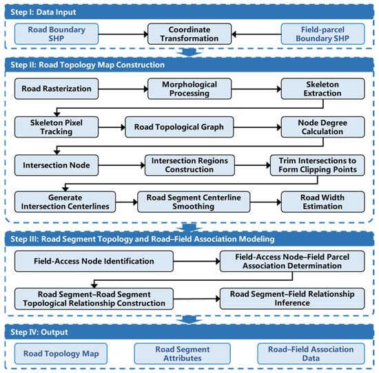
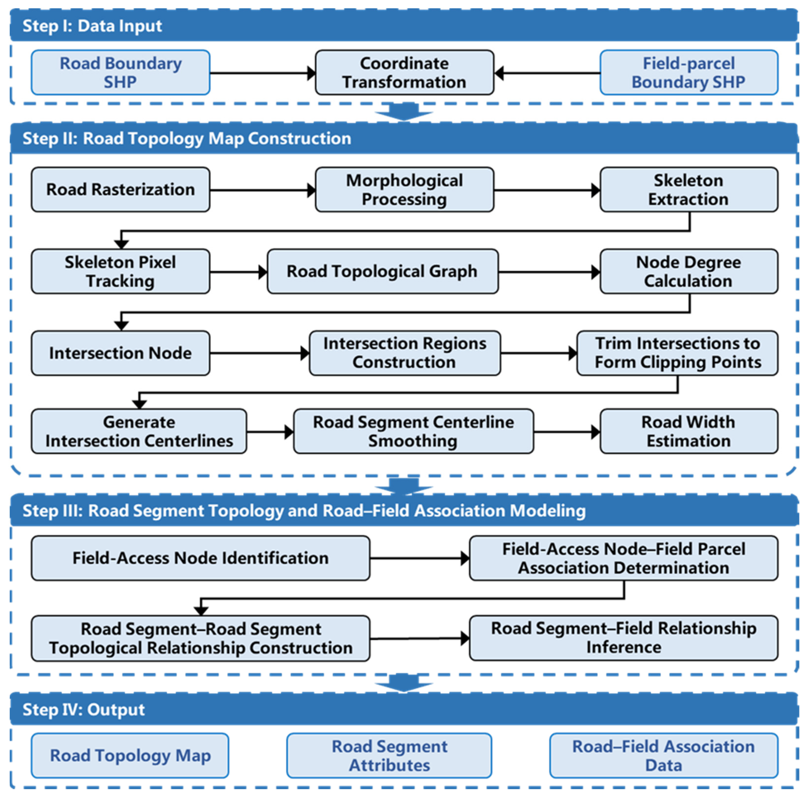
To address issues in unmanned farm navigation—such as irregular road boundaries, complex intersection layouts, large road-width variability, and incomplete field-accessibility information—this paper proposes a framework for constructing topological maps from road vector data (Figure 1). The framework sequentially performs road raster processing and skeleton-based centerline extraction, node–edge topological construction with segment partitioning, normal-sampling-based segment width estimation, and bidirectional modeling of associations between field-access nodes and farmland parcels. The outputs are structured road-network data that contain centerline coordinates, node–edge connectivity, and segment width fields, providing data for path planning and operation scheduling.

Figure 1. Workflow for constructing farmland road topological data. Step I: Input road and field boundaries and unify coordinates. Step II: Extract centerlines and compute segment-level attributes such as road width. Step III: Construct road-segment-to-road-segment and road-segment-to-field associations. Step IV: Export the road topological graph, segment attributes, and field association tables.

2.2. Problem Formulation

Let the road network be denoted by $R=\left\{R_k\right\}$ and the farmland parcels by $F=\left\{F_m\right\}$. Given $R$ and $F$, this study builds a road-network representation for unmanned-farm path planning and operation scheduling that encodes road connectivity, road-width attributes, and field-access relationships at entrances and exits. Specifically, the roads are converted into a node–edge topological graph, $G=\left(V,E\right)$, and each edge is assigned a length, $l_e$, and a segment width, $w_e$. Node types are determined by the degree, $d\left(\nu \right):d\left(\nu \right)=1$, or candidate field-access nodes, $d\left(\nu \right)=2$ for ordinary nodes, and $d\left(\nu \right)\ge 3$ for intersection nodes. Let $B\left(\nu ,\delta \right)$ denote the circular neighborhood of radius, $\delta$, centered at node $\nu$. If $F_m\cap B\left(\nu ,\delta \right)\ne \varnothing$, node $\nu$ is judged to have a field-access association with parcel, $F_m$. The method is finally evaluated jointly using centerline error, road-width error, and path-planning performance.

2.3. Road-Centerline Extraction and Road Segment-Structure Generation

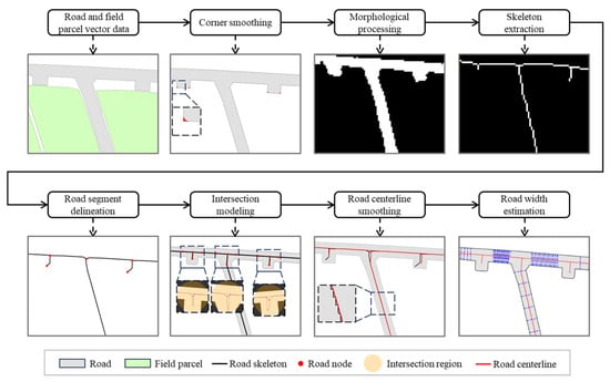
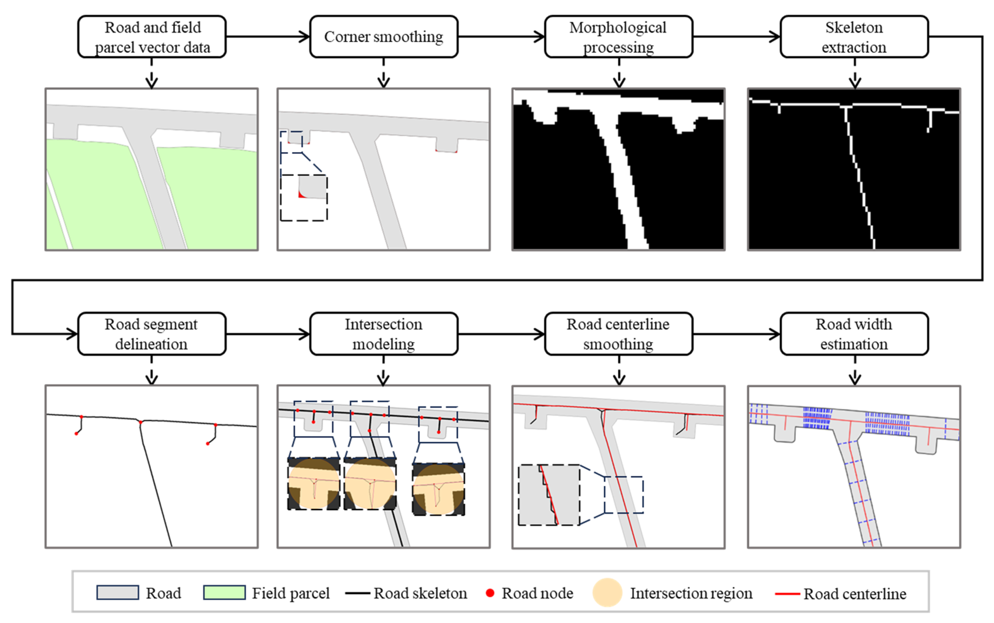
Figure 2 illustrates the main processing pipeline from road and field-parcel vector inputs to segment-level width attributes. Road boundaries are first rounded at ends, followed by morphological processing in the raster domain. The road skeleton is then extracted and vectorized into centerlines, after which road segments are delineated and intersections are modeled. Segment centerlines are smoothed, and segment widths are estimated by normal-direction sampling. The result is a structured road network that includes centerlines, nodes, and width information.

Figure 2. Workflow of road-centerline extraction, road-segment delineation, and road-width estimation.

2.3.1. Farm-Road Network Preprocessing

(1)

Fillet treatment of road-end pavement surfaces

Road vectors often exhibit flat-cut or sharp-corner boundaries at their ends; such geometry tends to produce spurious bifurcations and short spurs during skeleton extraction. To mitigate this, we first apply end rounding to the farm-road network: terminal sharp-corner regions are identified and then replaced with circular arcs so that the end boundaries become smoother.

(2)

Rasterization of road-network vector data

When farm-road vectors are rasterized directly, narrow roads, bends, and intersections often produce small holes, gaps, and jagged boundaries, which can lead to breaks or spurious branches during skeleton extraction. To reduce this effect, we first rasterize the roads (interior pixels = 1; exterior = 0); apply a closing operation, together with moderate dilation and erosion, to repair small gaps; suppress boundary jaggedness; and obtain a cleaner, more complete binary road mask.

2.3.2. Skeleton Extraction of the Farm-Road Network

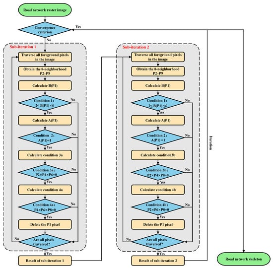
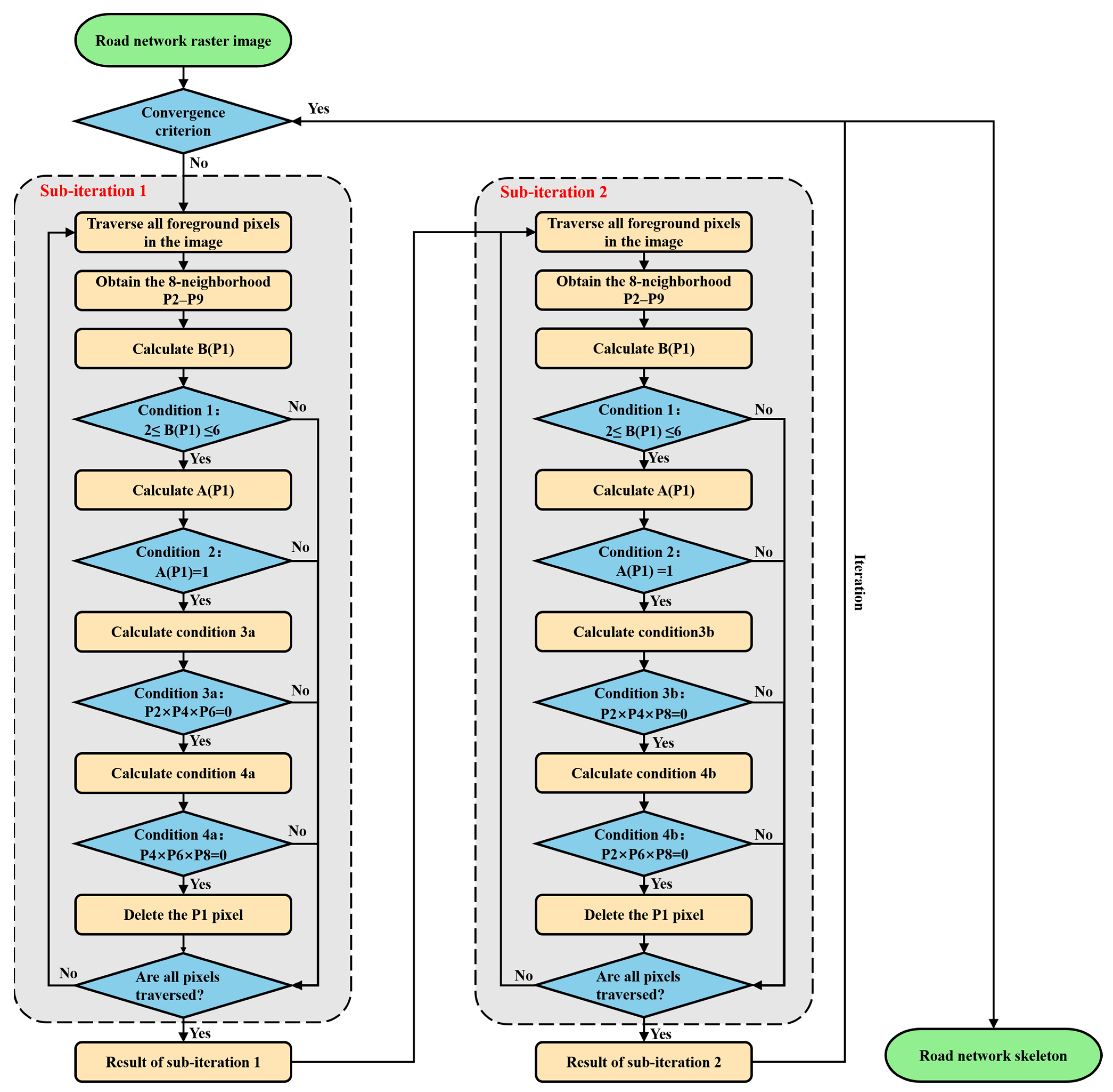
In narrow roads and intersection areas, skeleton extraction tends to produce short breaks, spurious branches, and shifted node locations, which in turn affects subsequent road segmentation and topology construction. To address this, we adopt a two-subiteration skeleton extraction method based on local neighborhood convolution and logical predicates (Figure 3). Let the processed road mask be $S^{(0)}=M^{\prime }$. In each iteration, boundary pixels to be removed are determined jointly by a $3\times 3$ neighborhood convolution and logical rules; boundary pixels are removed step by step while preserving connectivity and critical node structure, until convergence yields the skeleton grid, $S$.

Figure 3. Iterative skeleton extraction strategy based on local neighborhood convolution-based predicates.

For any pixel, $\left(i,j\right)$, its 8-neighborhood is defined in clockwise order as

$$p_2=S\left(i-1,j\right), p_3=S\left(i-1,j+1\right), p_4=S\left(i,j+1\right), p_5=S\left(i+1,j+1\right)$$

(1)

$$p_6=S\left(i+1,j\right), p_7=S\left(i+1,j-1\right), p_8=S\left(i,j-1\right), p_9=S\left(i-1,j-1\right)$$

(2)

The foreground pixel count in the 8-neighborhood is

$$B\left(i,j\right)={\displaystyle \sum _{k=2}^9{p}_k}$$

(3)

which can be computed by convolution as follows:

$$B=S\ast K_{sum},K_{sum}=\left(\begin{array}{ccc}1& 1& 1\\ 1& 0& 1\\ 1& 1& 1\end{array}\right)$$

(4)

Define the number of $0\to 1$ transitions along the cyclic sequence $\left(p_2,p_3,\dots ,p_9,p_2\right)$

$$A\left(i,j\right)={\displaystyle \sum _{k=2}^9\left(1-p_k\right)}{p}_{k+1},p_{10}=p_2$$

(5)

where $A\left(i,j\right)$ indicates that the foreground neighborhood forms a simply connected transition in the cyclic sense. In implementation, $A$ can be computed from the convolution responses of eight directional neighbor pairs combined with logical operations.

At iteration $t$, the input is $S^{\left(t\right)}$. Each iteration consists of two subiterations, which produce deletion masks $D_1$ and $D_2$, respectively, and the grid is updated in a mark-then-delete manner:

$$S^{\left(t+{\displaystyle \frac{1}{2}}\right)}=S^{\left(t\right)}\odot \left(1-D_1\right),S^{\left(t+1\right)}=S^{\left(t+{\displaystyle \frac{1}{2}}\right)}\odot \left(1-D_2\right)$$

(6)

where $\odot$ denotes element-wise multiplication.

For a candidate pixel to be deleted with $S(i,j)=1$, the following constraints must be satisfied simultaneously:

Neighborhood density constraint:

$$2\le B(i,j)\le 6$$

(7)

Single-connectivity constraint:

$$A(i,j)=1$$

(8)

Direction-preserving constraint (applied separately in the two subiterations):

Subiteration 1:

$$p_2{p}_4{p}_6=0, p_4{p}_6{p}_8=0$$

(9)

Subiteration 2:

$$p_2{p}_4{p}_8=0, p_2{p}_6{p}_8=0$$

(10)

Accordingly, the deletion masks are defined as follows:

$$D_1(i,j)=\mathbb{I}\left[S(i,j)=1\wedge \left(\mathrm{eq.}\left(7\right)\right)\wedge \left(\mathrm{eq.}\left(8\right)\right)\wedge \left(\mathrm{eq.}\left(9\right)\right)\right]$$

(11)

$$D_2(i,j)=\mathbb{I}\left[S(i,j)=1\wedge \left(\mathrm{eq.}\left(7\right)\right)\wedge \left(\mathrm{eq.}\left(8\right)\right)\wedge \left(\mathrm{eq.}\left(10\right)\right)\right]$$

(12)

where $\mathbb{I}\left[·\right]$ denotes the indicator function.

When no pixels are marked for deletion in either subiteration of a given iteration, i.e.,

$${‖D_1‖}_0+{‖D_2‖}_0=0$$

(13)

the skeleton is considered converged, and the final skeleton is obtained as

$$S=S^{\left(T\right)}$$

(14)

2.3.3. Road-Topology Construction and Road-Segment Delineation

To obtain a structured road-network representation, this study constructs a node–edge graph, $G=(V,E)$, from the skeleton, $S$. The procedure is as follows: first, centerlines are obtained by segment-wise tracing on the skeleton grid using local pixel degrees; then the start and end points of each centerline segment are mapped to graph nodes, and graph edges are generated from the segment connectivity; finally, road segments are defined by the edge set.

(1)

Road-network centerline construction

For each foreground pixel in the skeleton raster, we compute its local degree, $d(p)$: pixels with $d(p)=1$ are treated as segment endpoints, pixels with $d(p)\ge 3$ are treated as intersection points, and pixels with $d(p)=2$ are used to extend the path. Specifically, starting from endpoints and intersection points, we trace stepwise along skeleton pixels of degree 2 until a new endpoint or intersection is reached, yielding the set of centerline segments, $\left\{l_s\right\}$.

(2)

Node–edge graph construction

The centerline segment set, $\left\{l_s\right\}$, is processed segment by segment: for each segment, its start and end points are extracted and matched to the topological node set, $V$, under a snap-distance constraint. When the two ends of a segment map to distinct nodes, $u\ne v$, an edge, $e=(u,v)$, is added to the graph, and the corresponding centerline segment is stored as an edge attribute.

(3)

Node-degree classification and road-segment definition

Based on the constructed graph, $G=(V,E)$, the degree of each node in the graph is computed as follows:

$$deg(v)=\left|\left\{e\in E\left|\nu \in e\right.\right\}\right|$$

(15)

Nodes are classified by degree: $\mathrm{deg}(\nu )=1$ denotes an endpoint node, $\mathrm{deg}(\nu )=2$ a regular node, and $\mathrm{deg}(\nu )\ge 3$ an intersection node.

2.3.4. Intersection Region Modeling

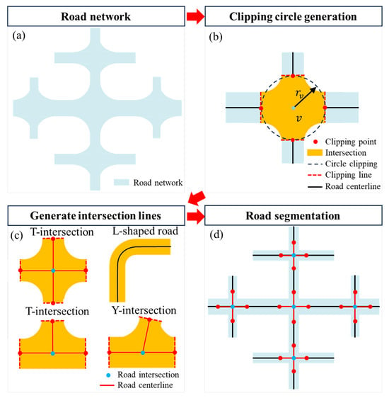
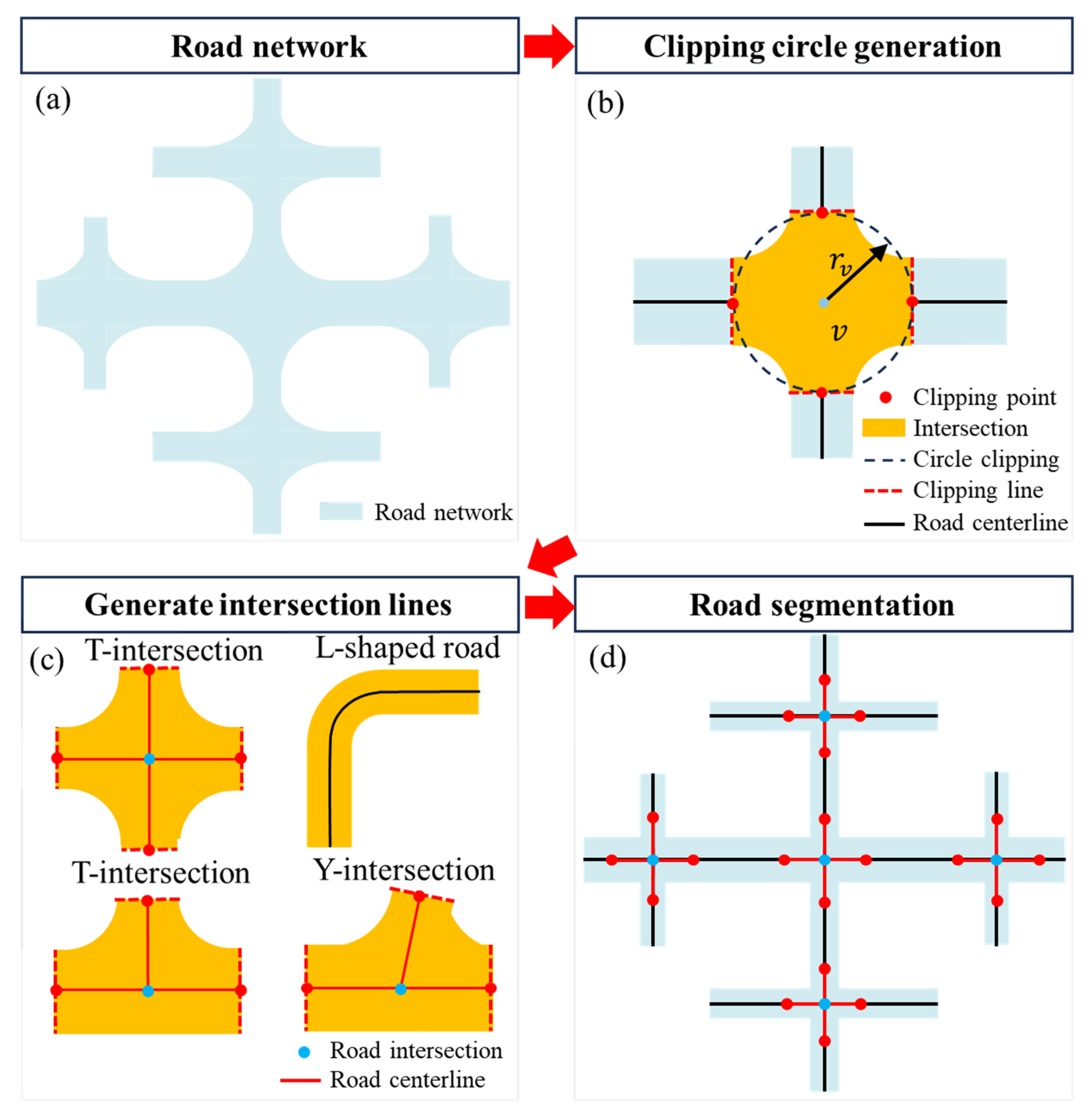
Intersections are critical regions in farm-road networks where multiple road segments meet (Figure 4a). To avoid mis-segmentation of neighboring road segments due to inappropriate intersection scales, this paper defines an intersection area at each intersection node in the initial road-network graph, $G=(V,E)$, and then performs road-segment partitioning and topological updates accordingly.

Figure 4. Modeling of intersection areas and reconstruction of the road-network topology. (a) Input road network and intersection areas; (b) generate intersection clipping circles and determine clipping points; (c) generate connecting line segments within the intersection area, applicable to T-intersections, cross-intersections, Y-intersections, and turning intersections; and (d) update centerlines and complete road-segment splitting and topological adjustment.

Let the intersection node be $\nu$, with graph degree satisfying $\mathrm{deg}(\nu )\ge 3$. The intersection region is defined as the circular area centered at $\nu$, with radius $r_{\nu }$ (Figure 4b):

$$J_{\nu }=Buffer(\nu ,r_{\nu })$$

(16)

Let $\left\{w_1,\dots ,w_{\mathrm{deg}\left(\nu \right)}\right\}$ denote the widths of the road segments incident to node $\nu$, and let ${\overline{w}}_{\nu }$ be their central value taken as the median. The intersection radius is defined as

$$r_{\nu }^{raw}=\alpha ·{\overline{w}}_{\nu }·\psi (deg(v))$$

(17)

where $\alpha \in (0,1]$ is a scaling coefficient, and $\psi \left(·\right)$ is a degree factor satisfying $\psi \left(3\right)=1$ and monotonically non-decreasing with degree. In this study,

$$\psi \left(d\right)=\left\{\begin{array}{cc}\begin{array}{c}1.0,\\ 1.4,\\ 1.6,\end{array}& \begin{array}{c}d=3,\\ d=3 \mathbf{or} 5,\\ d\ge 6,\end{array}\end{array}\right.$$

(18)

The final radius is obtained by applying lower- and upper-bound constraints:

$$r_v=\mathbf{clip}(r_{\nu }^{raw};r_{\min },r_{\max })$$

(19)

2.3.5. Centerline Smoothing

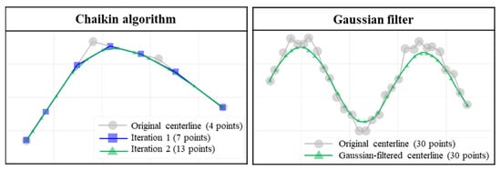
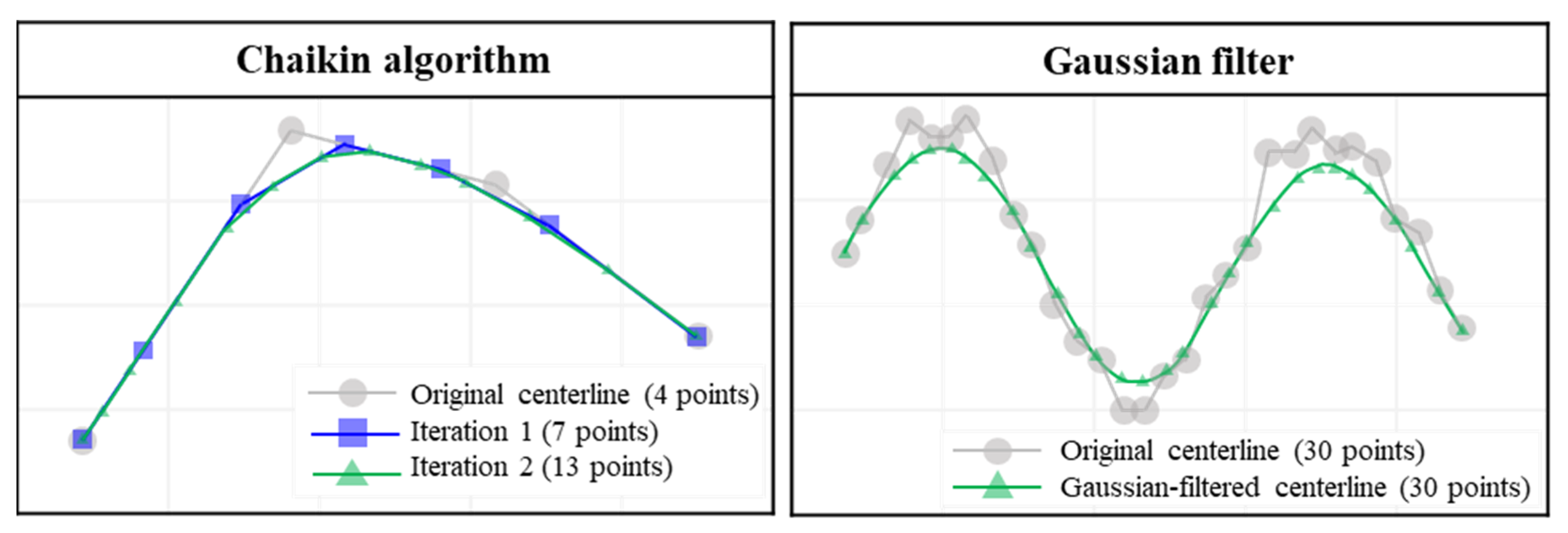
After raster skeletonization and vectorization, segment centerlines may still show local roughness and positional error. To improve the reliability of subsequent processing, each segment centerline is smoothed after segment identification and topological association (Figure 5). The smoothing procedure is as follows:

Figure 5. Chaikin iterative path-smoothing and Gaussian-filter path-smoothing algorithms.

Let $\{{\nu }_i{\}}_{i=1}^N$ denote the vertex sequence of the centerline for segment $e$. Before smoothing, polyline simplification is performed to remove redundant vertices using a threshold, ${ϵ}_s$. Piecewise sliding-window smoothing is then applied, and vertex positions are updated using Gaussian weights:

$${\tilde{\nu }}_i={\displaystyle \frac{{\displaystyle {\sum }_{k=-K}^K{\omega }_k{\nu }_{i+k}}}{{\displaystyle {\sum }_{k=-K}^K{\omega }_k}}}$$

(20)

where $K$ is the window radius, and ${\omega }_k$ represents distance-based weights. After window smoothing, spline fitting is applied to each piecewise segment to obtain smoother geometry. The smoothing procedure follows these rules: (1) endpoints at intersections remain fixed to avoid shifting intersection locations; (2) the displacement of any single vertex does not exceed ${\delta }_{\max }$; and (3) segments with large curvature are partitioned first and smoothed separately to preserve turning shapes. This strategy improves centerline quality without altering the road-network topology, providing a more stable input for subsequent road-width estimation.

2.3.6. Road-Width Estimation

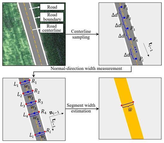
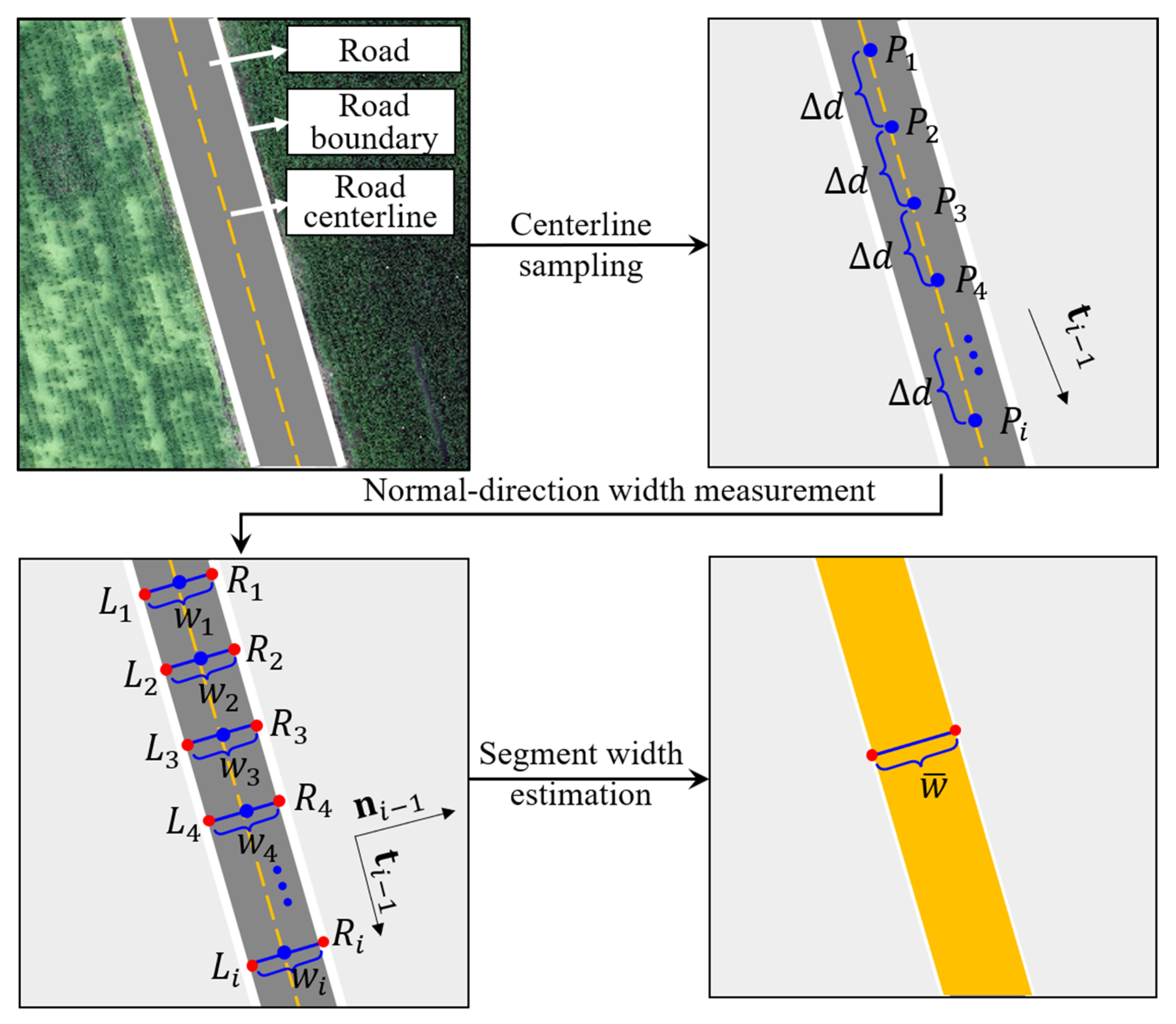
Road width is an important quantity characterizing the scale of farm roads. After the road-segment topology is built, this study measures width laterally along each segment centerline and computes local width from intersections with the road boundary (Figure 6).

Figure 6. Schematic of the road segment width-estimation procedure.

For each segmented road segment, sample points are taken along the centerline at a fixed spacing, yielding the sequence ${\left\{P_i\right\}}_{i=1}^N$. At each sample point, $P_i$, the local tangent vector, ${\mathbf{t}}_i$, of the centerline is used to construct the unit normal vector, ${\mathbf{n}}_i\left({\mathbf{n}}_i\perp {\mathbf{t}}_i\right)$. A local transversal is then constructed along ${\mathbf{n}}_i$ and intersected with the road boundary to obtain the left and right intersection points, $L_i$ and $R_i$. The width at that sample is defined as

$$w_i={‖L_i-R‖}_2$$

(21)

Because farm-road boundaries can be irregular, the width samples may contain outliers. Therefore, within each segment, outlier detection is applied to $\left\{{\omega }_i\right\}$, and width values that deviate strongly from the bulk of the distribution are removed. This yields a usable width sequence, ${\left\{{\omega }_i\right\}}_{i=1}^{N^{\prime }}$, from which segment-level width statistics are computed:

$$\overline{w}={\displaystyle \frac{1}{N^{\prime }}}{\displaystyle \sum _{i=1}^{N^{\prime }}{w}_i,s_w}=\sqrt{{\displaystyle \frac{1}{N^{\prime }-1}}{\displaystyle \sum _{i=1}^{N^{\prime }}{\left(w_i-\overline{w}\right)}^2}}$$

(22)

where $\overline{w}$ denotes the representative width of the segment, and $s_w$ denotes the spread of the width samples. The pointwise width sequence along the segment is also retained to describe how width varies along the segment. For segments whose width changes in a clearly piecewise manner, a sliding window and clustering are further used to partition the segment into sub-segments with more uniform width, and a representative width is assigned to each sub-segment.

2.4. Road-Segment Topology and Field-Association Modeling

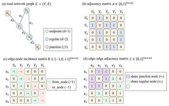
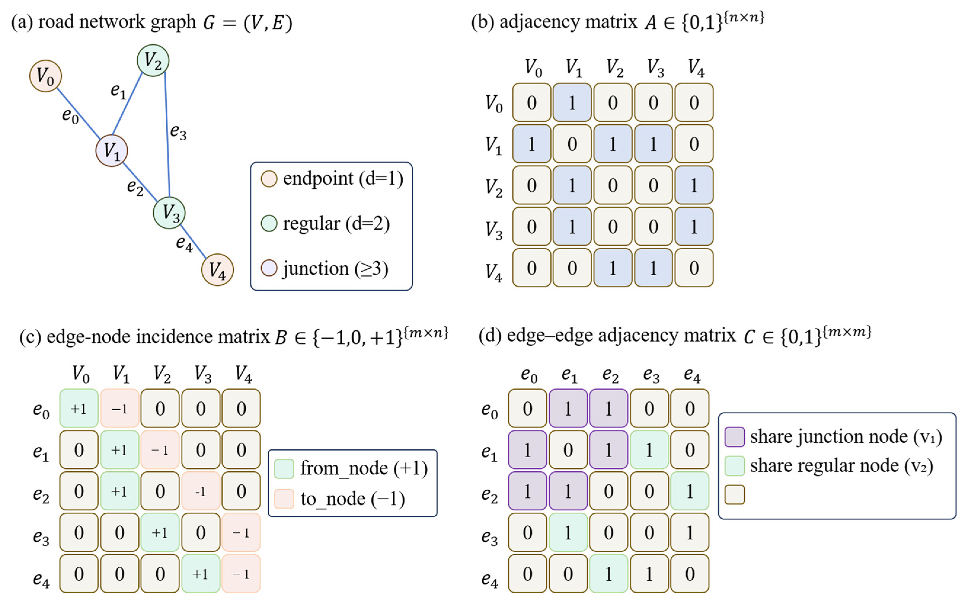
If a road network description only records how road segments connect to one another, it is difficult to meet the needs of agricultural machinery scheduling for field access points, field-to-field reachability, and cross-field path planning. For unmanned farm navigation, this study builds a road–field topological model on top of the constructed road network graph, jointly representing field-access nodes, road segments, and field parcels, and establishes bidirectional associations from road segments to fields and from fields to road segments (Figure 7).

Figure 7. Schematic of farm-road network graph representation and construction of adjacency relation matrices.

2.4.1. Construction of Segment-to-Segment Topological Relations

Segment-to-segment topological relations are defined on the edge set, $E$. For any two segments, $e_p=({\nu }_a,{\nu }_b)$ and $e_q=({\nu }_b,{\nu }_c)$, if they share node ${\nu }_b$, they are said to be topologically adjacent, denoted as $e_p\sim e_q$. For any node ${\nu }_i$, its incident edge set is defined as

$$E({\nu }_i)=\left\{e_j\in E\left|{\nu }_i\in e_j\right.\right\}$$

(23)

Then, the set of adjacent segments for segment $e_j=({\nu }_s,{\nu }_t)$ can be written as

$$N(e_j)={\displaystyle \underset{{\nu }_i\in \left\{{\nu }_s,{\nu }_t\right\}}{\cup }\left(E\left({\nu }_i\right)/\left\{e_j\right\}\right)}$$

(24)

where $N(e_j)$ denotes all segments that are directly connected to $e_j$.

2.4.2. Road-Segment–Field-Topological Relations

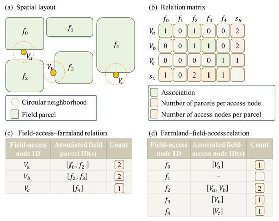
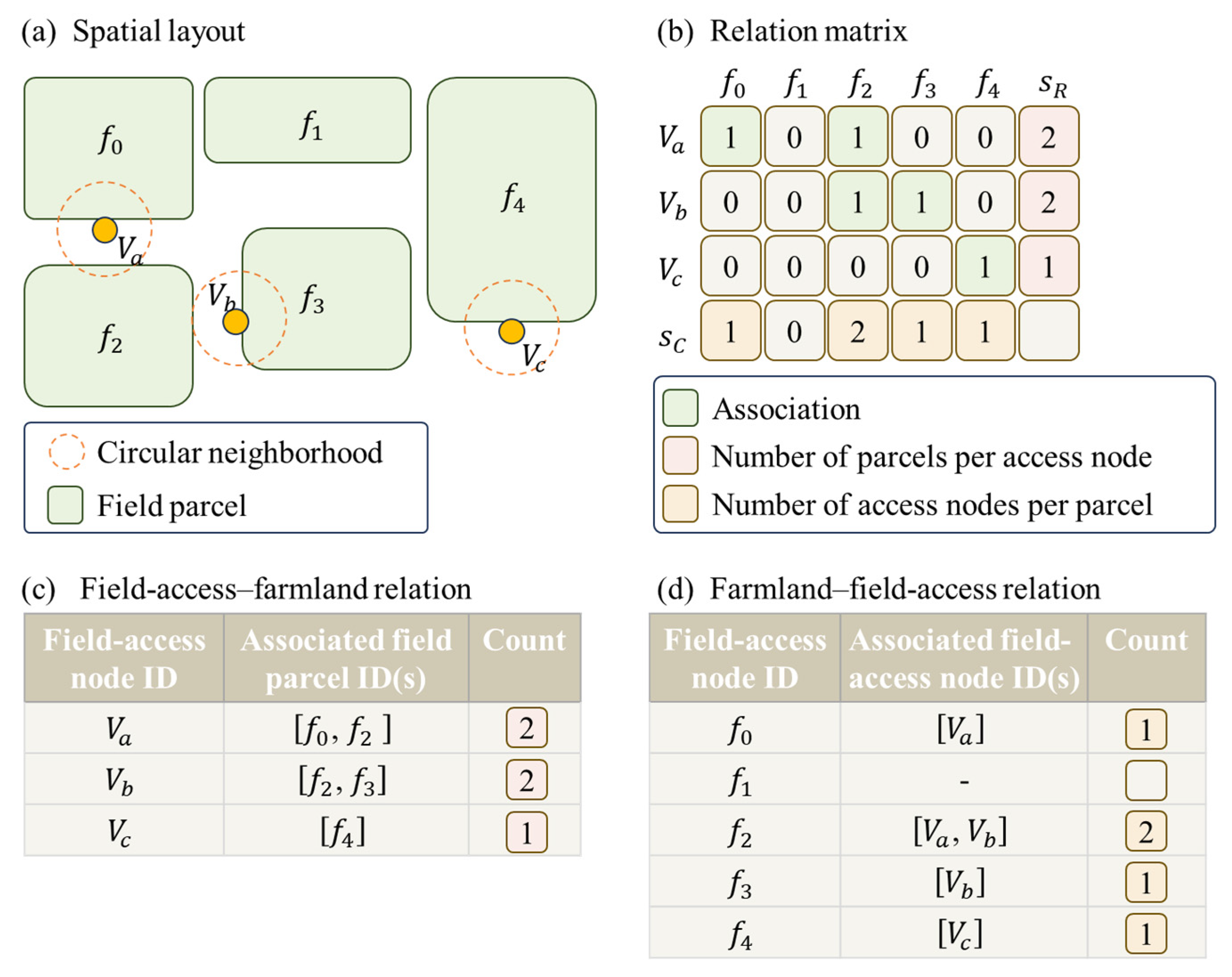
Connectivity among segments alone is insufficient to support farm operation scheduling. Therefore, on the basis of the road-network graph, $G=(V,E)$, and field-parcel vector data, this study selects road-end nodes as candidate locations for field access points and, together with node–edge associations, establishes road-segment–field associations according to whether a circular neighborhood of radius, $\delta$, around each field-access node intersects a field parcel (Figure 8). This procedure yields two complementary tables—node–field and field–node—and further yields road-segment–field mappings.

Figure 8. Construction of field-access node–field topological associations and relational tables.

(1)

Field-access node identification

Nodes satisfying $\mathbf{deg}(\nu )=1$ in the road network are treated as candidate field-access nodes, denoted $V_{entry}\subseteq V$. In farm-road settings, such nodes typically correspond to road ends and are incident to exactly one segment. If a candidate node, $\nu \subseteq V_{entry}$, and a field parcel, $P$, satisfy the proximity condition, a field-access association is considered to exist between them. Because the incident edge at $\nu$ is unique, node–field relations can be mapped to segment–field relations.

(2)

Node–field association rule

For node $\nu$, define a circular neighborhood $B\left(\nu ,\delta \right)$ centered at $\nu$ with radius, $\delta$. For any field parcel, $P$, if

$$P\cap B(v,\delta )\ne \varnothing$$

(25)

then node $\nu$ is judged to have a field-access association with field parcel, $P$. Parameter $\delta$ controls the proximity scale and is set according to typical spacing between roads and field-parcel boundaries in this study.

(3)

Bidirectional relational tables

Based on the above rule, two complementary tables are built.

The node–field table uses $\nu \subseteq V_{entry}$ as the primary key and records

$$F\left(\nu \right)=\left\{P\left|P\cap B(v,\delta )\ne \varnothing \right.\right\}$$

(26)

together with $n_v=\left|F\left(\nu \right)\right|$. Each record contains a node ID, the list of associated parcel IDs, and $n_v$.

The field–node table uses field parcel, $P$, as the primary key and records

$$E\left(P\right)=\left\{\nu \subseteq V_{entry}\left|P\cap B(v,\delta )\ne \varnothing \right.\right\}$$

(27)

Together, the node–field and field–node representations establish segment-level bidirectional road–field associations: roads can be queried for accessible parcels, and parcels for candidate field-access nodes.

(4)

Deriving segment–field relations

For any field-access node, $\nu \subseteq V_{entry}$, let $e_v$ denote its unique incident segment in the graph. If $\nu$ and field parcel, $P$, satisfy the field-access association rule, then $e_v$ is assigned as a segment corresponding to $P$. Consequently, for any segment, $e$, its associated field-parcel set is determined from the field parcels associated with field-access nodes on $e$ that belong to $V_{entry}$; for any field parcel, $P$, its associated segment set is the union of segments corresponding to all field-access nodes that satisfy the rule. The resulting road–field representation contains both topological information and parcel identifiers within one data system, facilitating unified reading by scheduling modules.

2.5. Parameter Settings and Implementation Settings

The key parameters and implementation settings used for road rasterization, skeleton extraction, intersection modeling, width estimation, road–field association, and centerline smoothing are summarized in Table 1.

Table 1. Main parameter settings in the proposed method.

Parameter	Value
Raster resolution	0.05 m
Morphological structuring element	3 × 3
Corner-angle threshold	150°
Fillet-radius ratio	0.15
Intersection buffer coefficient	0.7
Intersection degree factor	1.0/1.4/1.6
Intersection radius bounds	3.5 m, 30.0 m
Width samples per segment	10
Tangent estimation distance	1.0 m
Field-access association radius	10.0 m

All settings were fixed across the three study areas. The raster resolution of 0.05 m matches the ground sampling distance of the UAV orthoimagery. End filleting used a corner angle threshold of 150° and a fillet radius ratio of 0.15. The intersection buffer coefficient (0.7), degree factor, and radius bounds jointly define intersection clipping. Width estimation used 10 samples per segment and a 1.0 m tangent offset. The field-access association radius was set to 10.0 m according to typical road–field spacing in the digitized data. Centerlines with more than 10 vertices were smoothed with Gaussian filtering; shorter polylines were smoothed with the Chaikin method.

3. Results

3.1. Study Area and Dataset Construction

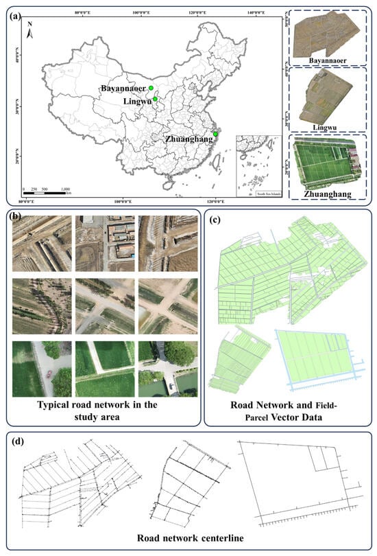
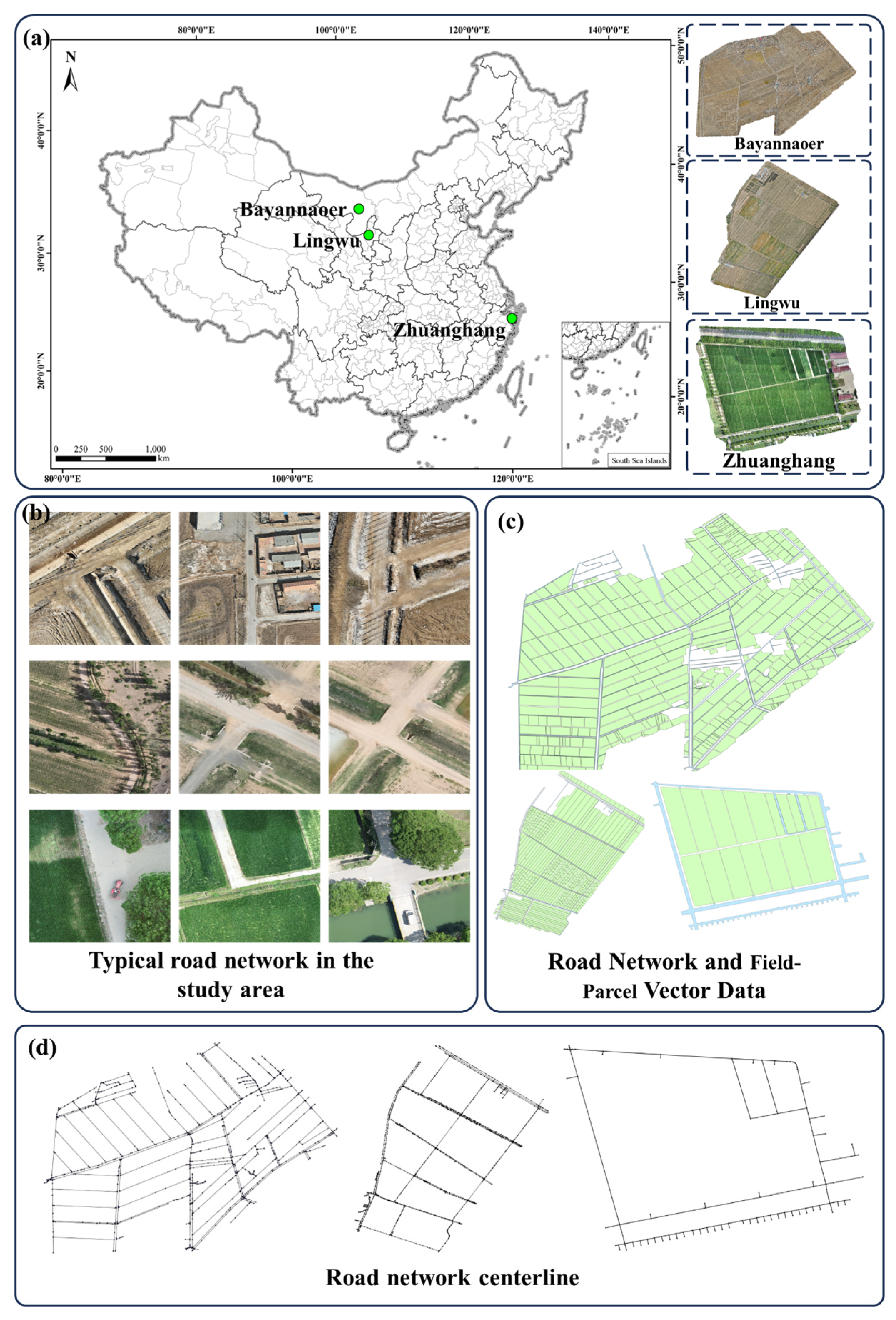
This study used three typical farm operation areas—Zhuanghang, Shanghai (121.37769°E, 30.89058°N); Bayannaoer (107.25863°E, 40.68303°N); and Lingwu (106.28351°E, 38.11878°N)—to build the experimental dataset (Figure 9a). Low-altitude imagery of the three areas was collected with a DJI Mavic 3 Multispectral unmanned aerial vehicle (UAV). The platform carries a 20 MP RGB camera, a multispectral camera, and a real-time kinematic (RTK) positioning module, and is suitable for fine-scale mapping of field roads and field-parcel boundaries. Flights were conducted at an altitude of 35 m, with 80% forward overlap and 75% side overlap, and a flight speed of 15 m/s. Imagery was acquired under clear or lightly cloudy conditions, and RTK status was checked before takeoff to support georeferencing and mosaic accuracy. After acquisition, DJI Terra was used for aerial triangulation, mosaicking, and orthorectification to produce high-resolution orthoimagery.

Figure 9. Study area locations and dataset composition: (a) geographic distribution of the study areas across China; (b) remote-sensing imagery of the three regions; (c) field-parcel and road vector data; and (d) manually annotated reference road-network centerlines.

As shown in Figure 9b, roads in the three areas include main field roads, farm tracks, and entrance segments connecting cropland to the road network; they contain both relatively long straight segments and shorter intersection segments, with T-intersections, cross-intersections, and irregular intersections. These characteristics increase the difficulty of centerline extraction, road segmentation, and intersection handling. Field-parcel polygons and road polygons for the three areas were digitized in ArcGIS Pro 3.0.1, as shown in Figure 9c.

Across the three areas, there are 1015 farmland parcels totaling 939.5 ha and 37.7 ha of road area. The manually annotated reference network contains 2667 centerline edges and 2629 nodes, including 279 intersection nodes, with a total centerline length of 93.8 km (Table 2). Overall, the Zhuanghang area is smaller in extent; Bayannaoer and Lingwu cover larger areas with longer total centerline length and more complex road-network layouts. After completing the vector data shown in Figure 9c, reference centerlines were further annotated to obtain the road network in Figure 9d. The reference data are organized in three layers: the first provides centerline geometry as the baseline; the second records node–edge connectivity and node types; and the third records segment length, width, and derived attributes.

Table 2. Summary statistics of farmland parcels, roads, and reference centerlines for the study areas.

Study Area	Parcels (n)	Parcel Area (ha)	Road Area (ha)	Edges (n)	Nodes (n)	Intersection Nodes (n)	Centerline Length (km)
Bayannaoer	458	321.2	18.1	1076	1048	128	48.8
Lingwu	540	613.2	18.8	1457	1450	100	42.9
Zhuanghang	17	5.1	0.9	134	131	51	2.1
Total	1015	939.5	37.7	2667	2629	279	93.8

3.2. Comparative Evaluation of Road-Network Centerline Extraction Methods

To ensure a fair comparison, all compared methods shared the same preprocessing pipeline before skeleton extraction. Road polygons were first rasterized at the same raster resolution, and the resulting binary masks were processed using the same morphological operations. The same preprocessed road masks were then used as input for all skeletonization methods, including the medial-axis transform, Lantuéjoul, Zhang–Suen, Guo–Hall, distance-transform, Voronoi, Lee, and the proposed method; thus, the comparison reflects differences in skeletonization strategies rather than differences in preprocessing. Evaluation used bidirectional point-to-line distances: the shortest distance from the predicted centerline to the union of reference centerlines was denoted predicted-to-ground-truth distance (Pred→GT), and the shortest distance from reference centerlines to the union of predicted centerlines was denoted GT→Pred. Errors from both directions were merged to compute symmetric mean error (Sym Mean), symmetric 50th-percentile error (Sym P50), symmetric 95th-percentile error (Sym P95), and symmetric maximum error (Sym Max) (Table 3), and directional quantiles were reported separately (Table 4).

Table 3. Comparison of centerline errors across skeletonization methods.

Method	Sym Mean	Sym P50	Sym P95	Sym Max	Pred→GT Mean	GT→Pred Mean
Medial axis	0.114	0.052	0.474	4.560	0.091	0.137
Lantuéjoul	0.157	0.063	0.605	6.076	0.121	0.254
Zhang–Suen	0.115	0.048	0.467	4.021	0.104	0.126
Guo–Hall	0.121	0.058	0.451	3.971	0.100	0.143
Distance-transform	2.154	0.155	11.587	29.681	0.057	3.721
Voronoi	0.115	0.047	0.471	2.857	0.109	0.120
Lee	0.115	0.049	0.472	2.723	0.108	0.123
Ours	0.094	0.045	0.350	4.899	0.077	0.111

Table 4. Directional point-to-line error distributions across skeletonization methods.

Method	P→G P50	P→G P95	P→G Max	G→P P50	G→P P95	G→P Max
Medial axis	0.051	0.323	2.092	0.053	0.616	4.560
Lantuéjoul	0.063	0.461	2.483	0.062	1.233	6.076
Zhang–Suen	0.049	0.379	2.734	0.047	0.638	4.021
Guo–Hall	0.059	0.343	1.487	0.057	0.686	3.971
Distance-transform	0.041	0.162	0.656	1.607	16.230	29.681
Voronoi	0.048	0.410	2.857	0.046	0.638	2.518
Lee	0.050	0.379	2.723	0.048	0.638	2.530
Ours	0.043	0.273	2.734	0.047	0.448	4.899

As shown in Table 3, the proposed method (ours) achieves the smallest Sym Mean (0.094 m) and the smallest Sym P50 (0.045 m), with a Sym P95 of 0.350 m. Compared with mainstream baselines (medial axis transform, Zhang–Suen, Guo–Hall, Voronoi, and Lee), whose Sym Mean values cluster between 0.114 m and 0.121 m, the proposed method reduces the Sym Mean by approximately 17–22%, indicating smaller centerline positional deviation over the full road network. At high quantiles, Lantuéjoul exhibits elevated Sym P95 (0.605 m) and Sym Max (6.076 m), suggesting larger errors in some locally complex regions. The distance-transform skeleton yields a much higher Sym Mean (2.154 m) and Sym P95 (11.587 m) than the other methods, indicating a pronounced heavy tail in its error distribution.

Table 4 further reveals directional differences. The distance-transform skeleton shows small quantile errors in the Pred→GT direction (P95 = 0.162 m), but much larger errors in the GT→Pred direction (P95 = 16.230 m; Max = 29.681 m). This indicates that parts of the extracted centerlines can be locally close to the reference, while a substantial portion of the reference network is not adequately represented. By contrast, the proposed method is more balanced across directions: Pred→GT P95 = 0.273 m and GT→Pred P95 = 0.448 m; and at the mean level, Pred→GT Mean = 0.077 m and GT→Pred Mean = 0.111 m, with a directional gap of 0.034 m. These results suggest that the proposed method better balances “prediction deviation” and “reference coverage.”

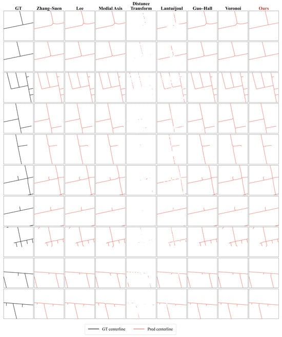
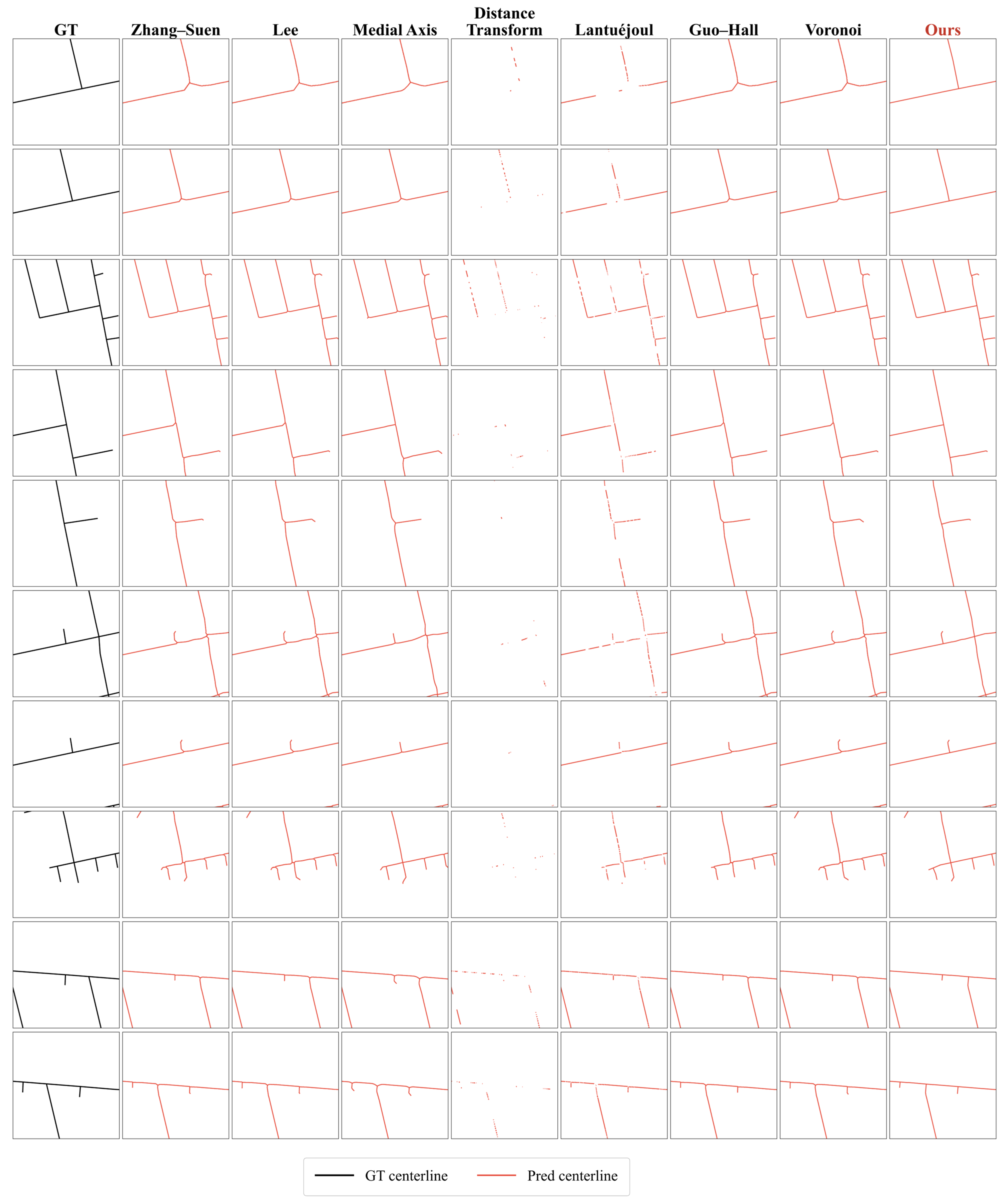
The qualitative comparison in Figure 10 is consistent with the quantitative results in Table 3 and Table 4. Across representative intersections, curves, road ends, and narrow branch connections, most methods can recover the main road direction, but their local stability differs. The distance-transform and Lantuéjoul methods show more fragmented or discontinuous centerlines in several cases, especially near intersections and road ends. The Zhang–Suen, Lee, Guo–Hall, medial-axis, and Voronoi methods generally preserve the main skeleton structure, but they still produce short spurs, local shifts, or redundant branches around irregular intersections and terminal road regions. In comparison, the proposed method produces centerlines that are closer to the reference centerlines in most examples and better preserves branch continuity while reducing spurious local branches.

Figure 10. Local comparison of eight skeletonization methods at representative locations (intersections, curves, and road ends). The first column shows the GT centerline; columns 2–9 show each method’s prediction.

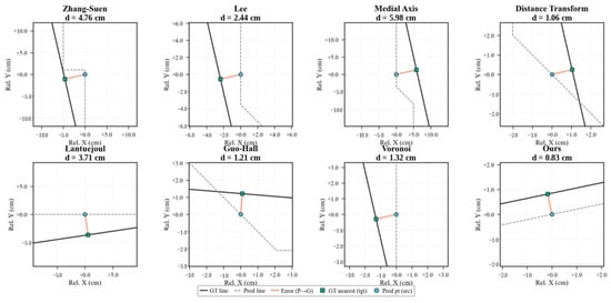
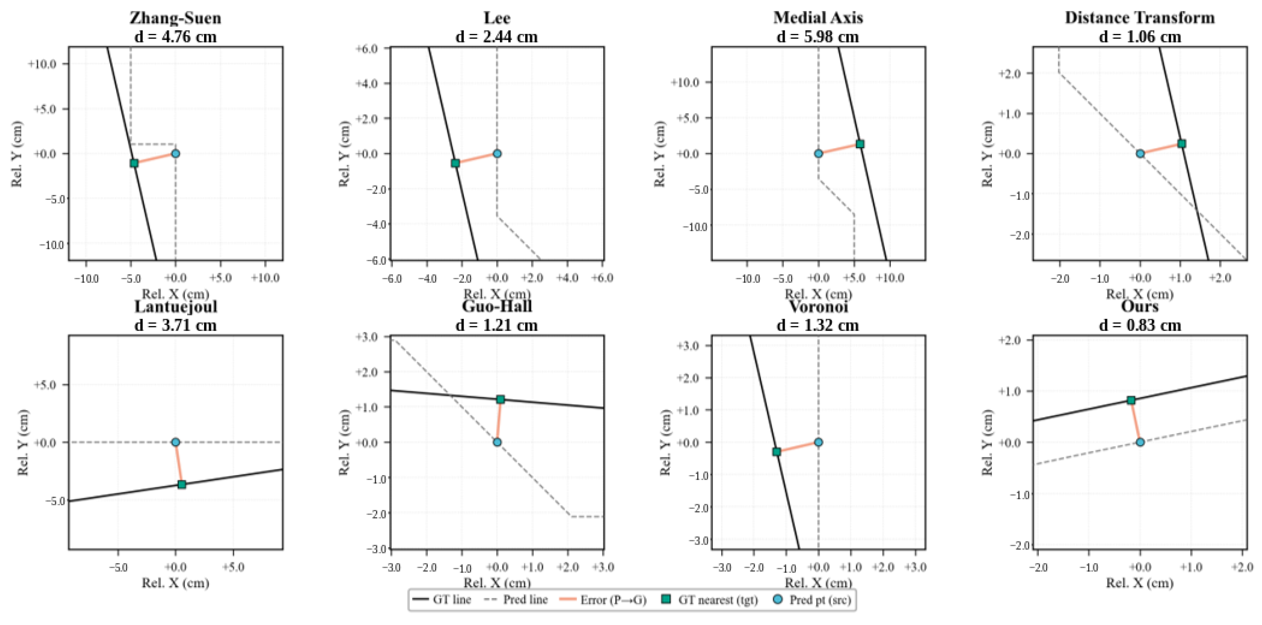
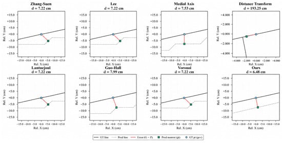
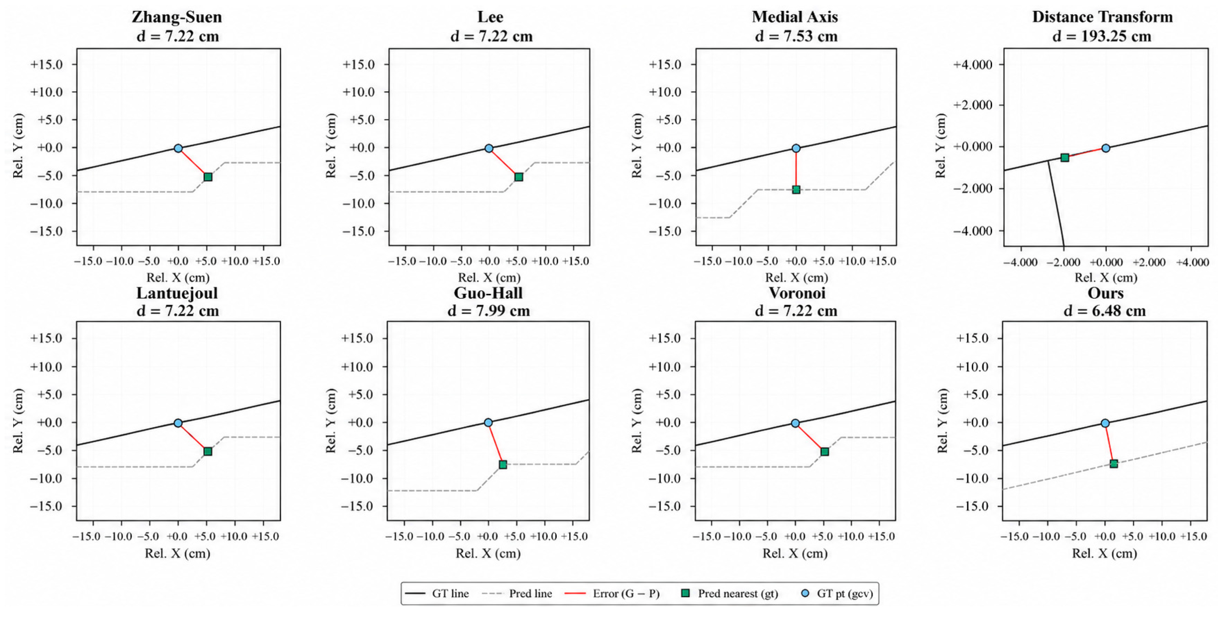
Figure 11 and Figure 12 further illustrate the two-directional point-to-line error measures. In Figure 11 (Pred→GT), errors are generally small for all methods, and the local error of the proposed method is 0.83 cm. In Figure 12 (GT→Pred), most methods have local errors of approximately 6–8 cm, and the proposed method has a local error of 6.48 cm. In contrast, the distance-transform skeleton shows a much larger error of 193.25 cm at the same location, reflecting missing segments or discontinuities in that region.

Figure 11. Point-to-line matching errors from predicted centerlines to reference centerlines (Pred→GT) at a selected farm-road location for Zhang–Suen, Lee, medial axis, distance transform, Lantuéjoul, Guo–Hall, Voronoi, and the proposed method. Each panel shows the predicted and reference centerlines, a sample point on the predicted centerline; the nearest point on the reference centerline; and the local error distance, d.

Figure 12. Point-to-line matching errors from reference centerlines to predicted centerlines (GT→Pred) at the same location for the same eight skeletonization methods. Each panel shows the reference and predicted centerlines; a sample point on the reference centerline; the nearest point on the predicted centerline; and the local error distance, d.

Taken together, Table 3 and Table 4 and Figure 10, Figure 11 and Figure 12 show that bidirectional centerline errors reveal missing or misaligned segments that a single-direction summary can overlook. Evaluation should consider not only whether the extracted centerlines are close to the reference centerlines (Pred→GT), but also whether the extracted centerlines adequately represent the reference network (GT→Pred). The proposed method maintains low errors in both directions and produces more stable local centerline structures, providing a more reliable centerline basis for subsequent road-width estimation and path planning.

3.3. Road Segment Width-Estimation Results

Table 5 reports the road segment width-estimation errors. Ground-truth widths were generated from manually checked reference road segments. For each segment, the manually annotated centerline served as the sampling baseline; normal cross-sections were constructed along the segment to intersect the corresponding road-polygon boundary. The distances between the two boundary intersections were recorded as width samples, and the median of the valid samples was taken as the segment-level ground-truth width. Width errors were obtained by comparing the estimated segment widths with these ground-truth values.

Table 5. Road width-estimation errors (m).

MAE	RMSE	MedianAE	P90 AE	P95 AE
0.032	0.060	0.007	0.073	0.085

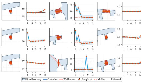
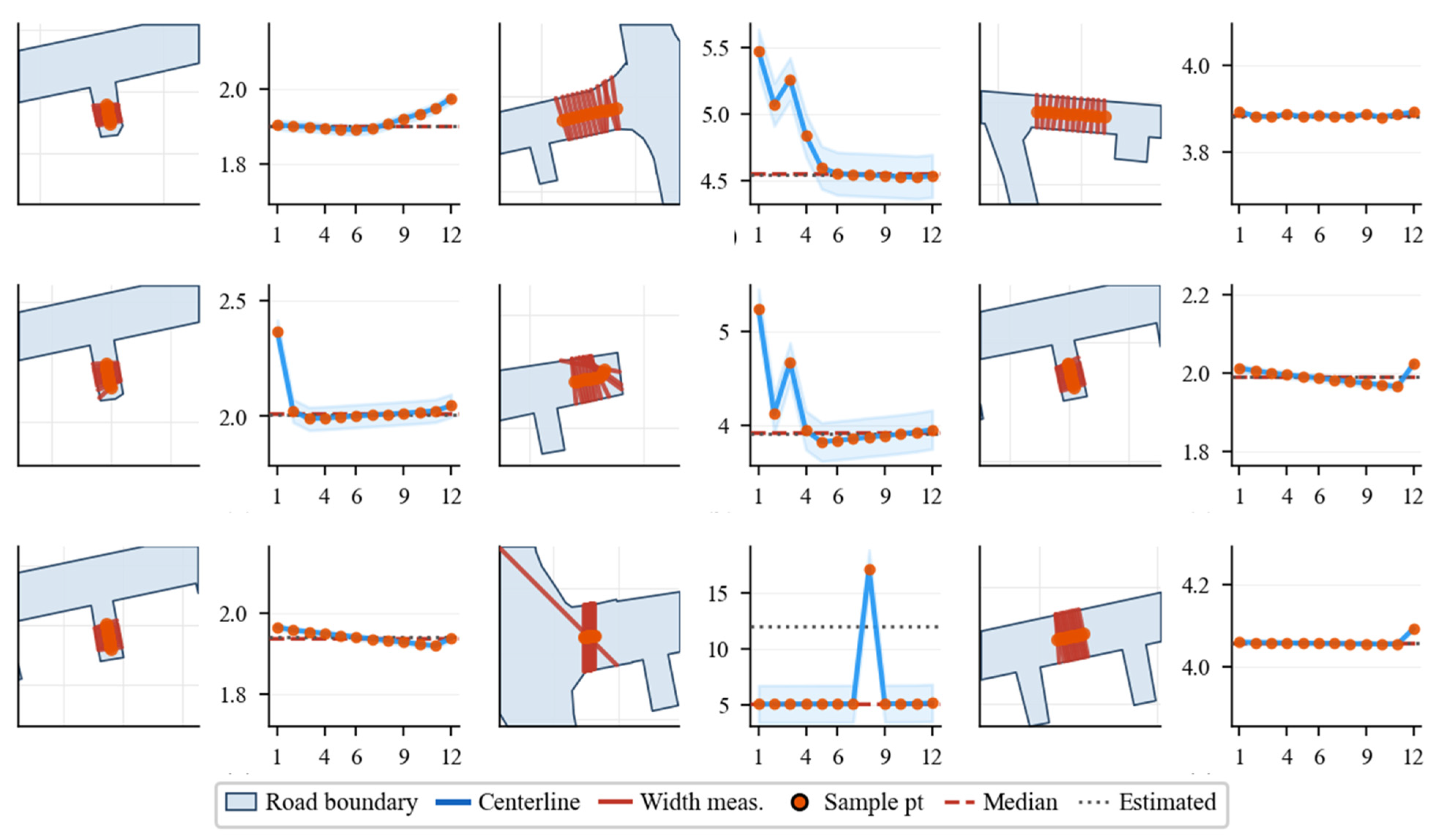
For the proposed method, MAE is 0.032 m, RMSE is 0.060 m, and Median Absolute Error (MedianAE) is 0.007 m, indicating that errors for most segments are on the order of centimeters. At the same time, RMSE is clearly higher than MAE, and 90th percentile absolute error (P90) (0.073 m) and 95th percentile absolute error (P95) (0.085 m) are much higher than the median error, showing a right-skewed error distribution: overall errors are small, but a small number of segments still have relatively large errors.

As shown in Figure 13, width errors are mainly related to location along the segment. On straight segments and where boundaries are relatively regular, pointwise width varies little, and the estimated width is close to most sampled values. Near intersections or where the road-width changes rapidly, cross-sections may pass through intersection openings, causing occasional very large sampled widths. After removing outlying width samples, the influence of spike samples on the segment-level representative width is reduced; however, intersections and rapidly changing widths can still produce a small number of large errors, so P90 and P95 remain higher than the median. This matches the pattern of a low MedianAE together with relatively higher P90 and P95.

Figure 13. Road-width sampling and segment-level estimation for farm-road segments with different widths and geometries. Left: Road boundary, centerline, normal-direction width measurements, and sample points. Right: Pointwise width values along the segment with the median and estimated representative width.

For most straight segments, the estimated widths are accurate to within a few centimeters, so each road edge can be assigned a width, and narrow segments can be excluded before path search. Larger errors are concentrated near intersections, where cross-sections may cut through junction openings; this keeps P90 and P95 above the median. Tighter width sampling or intersection masking in those regions would be needed to reduce the remaining high-percentile errors.

3.4. Ablation-Study Results

To analyze how each key processing module affects topological-map construction, we conducted ablation experiments on the same dataset under identical parameter settings. Using the full pipeline as the baseline, we separately removed (i) road-end filleting, (ii) intersection-area modeling, and (iii) skeleton centerline smoothing, and compared centerline geometric error, road segment-width error, and path-planning success rate across configurations. In the ablation study, path planning was evaluated for road-to-road tasks between graph nodes on the constructed network, without field-parcel attachment. Centerline error is reported as the symmetric bidirectional point-to-line distance mean; width error is reported as the MAE and 95th-percentile absolute error (P95) of road segment-width estimates. Results are summarized in Table 6.

Table 6. Ablation-experiment results.

Configuration	Sym Mean (m)	Sym P95 (m)	Pred→GT Mean (m)	GT→Pred Mean (m)	Width Error (m)	Width P95	Path Success Rate
Without end filleting	0.139	0.690	0.139	0.139	0.032	0.069	50%
Without intersection-area modeling	0.139	0.425	0.140	0.138	0.033	0.104	100%
Without skeleton smoothing	0.098	0.392	0.083	0.114	0.038	0.108	100%
Full method	0.094	0.350	0.077	0.111	0.032	0.085	100%

As shown in Table 6, removing end filleting increases the symmetric centerline error from 0.094 m to 0.139 m and the Sym P95 from 0.350 m to 0.690 m, and reduces the path-planning success rate from 100% to 50%. This indicates that road-end geometry directly affects endpoint identification and skeleton stability. Without filleting, flat-cut or sharp corners at road ends tend to produce short spurs, shifted endpoints, or spurious bifurcations during skeleton extraction, which degrades matching between terminal nodes and field access points. Therefore, this module has a larger impact on skeleton quality and path connectivity than on width accuracy. Notably, the configuration without end filleting yields the lowest Width P95 (0.069 m), even lower than the full method (0.085 m). This occurs because end filleting replaces sharp terminal boundaries with circular arcs, which can shift a small number of width cross-sections near road ends and slightly increase high-percentile width errors at those locations. Without filleting, the original road-end boundaries happen to produce width samples closer to the reference. However, this configuration simultaneously degrades centerline accuracy and path-planning success (50%), confirming that end filleting involves a trade-off: it improves terminal topology at the cost of a minor increase in tail-width error near road ends.

Removing intersection-area modeling also increases the Sym Mean to 0.139 m, with a Pred→GT Mean and GT→Pred Mean of 0.140 m and 0.138 m, respectively, both higher than the full method. This suggests that intersection-area modeling improves segmentation of centerline segments near intersections and mitigates redundant nodes and boundary-cut biases caused by multi-branch convergence. Although the path success rate remains 100% under this configuration, centerline geometric error and the quality of node–edge representation deteriorate, implying that intersection-area modeling mainly affects geometric consistency of the topology rather than necessarily making paths unreachable. Width P95 under this configuration rises to 0.104 m, indicating that without intersection-area clipping, some width cross-sections near multi-branch junctions traverse intersection openings and inflate high-percentile width errors.

Removing skeleton smoothing increases centerline error from 0.094 m to 0.098 m, a relatively small change; however, width MAE increases from 0.032 m to 0.038 m. This indicates that smoothing has a limited effect on overall centerline placement but a clearer effect on normal-direction width sampling. Without smoothing, skeleton centerlines exhibit local jags and abrupt direction changes, which perturb tangent and normal estimation at sample points and shift intersection points between cross-section lines and road boundaries, thereby increasing road width-estimation error. This is further reflected in Width P95, which increases from 0.085 m to 0.108 m, the highest among all configurations, confirming that smoothing is the module most directly responsible for reducing tail-width errors.

Overall, the three modules influence different aspects of the pipeline. End filleting mainly affects road-end identification and path connectivity; intersection-area modeling mainly affects centerline segmentation and node–edge topology expression at intersections; skeleton smoothing mainly affects road-width estimation under normal-direction sampling. The Width P95 results reveal that the three modules affect the width-error tail differently: removing smoothing or intersection modeling increases Width P95 above 0.10 m, whereas removing end filleting actually lowers it to 0.069 m due to unmodified terminal boundaries. The full method does not achieve the lowest Width P95, but it attains the best balance across centerline error, width MAE, width P95, and path-planning success, indicating that the combined modules improve the overall usability of the farm-road topological map.

3.5. Path-Planning-Evaluation Results

To evaluate the performance of the constructed topological map in navigation tasks, this study assesses two aspects: (1) whether a feasible path can be obtained; and (2) the deviation between the predicted path length and the ground-truth path length. Four task types are considered: road-to-road, field-to-road, road-to-field, and field-to-field.

As shown in Table 7, all 50 test tasks yielded a feasible path, giving an overall success rate of 100.0% across all four task categories. This confirms that the node–edge topology and bidirectional field-access mapping provide sufficient connectivity for path planning. Regarding path-length deviation, the mean relative error is 4.63%; the median is 0.89%; P90 and P95 are 10.94% and 14.92%, respectively; and the maximum is 59.03%. This maximum error occurred in a short road-to-road task (GT path length: 40.5 m) near a T-shaped intersection, where the skeleton-derived node was displaced approximately 13 m from its ground-truth position due to asymmetric road-boundary geometry. The resulting absolute detour was only approximately 30 m, adding less than 22 s of travel time at a typical field speed of 5 km/h. The high relative value is attributable to the short reference path length rather than a fundamental topological failure. The error distribution indicates that most tasks exhibit small length deviations, while a few outliers arise when the start or end point is located near an intersection or a field-parcel boundary; under such conditions, the placement of field-access nodes and the segmentation near intersections affect how endpoints attach to the network, increasing the difference between the predicted and ground-truth path lengths. The proposed method thus performs well in terms of path existence, while path-length accuracy near intersections and field-access boundaries warrants further optimization of node placement strategies.

Table 7. Path-planning results.

Metric	Value
Total number of test cases	50
Number of successful cases	50
Overall success rate	100.0%
Relative error of path length, mean	4.63%
Relative error of path length, median	0.89%
Relative error of path length, P90	10.94%
Relative error of path length, P95	14.92%
Relative error of path length, maximum	59.03%
Road-to-road cases/success rate	15/100%
Field-to-road cases/success rate	10/100%
Road-to-field cases/success rate	10/100%
Field-to-field cases/success rate	15/100%
Time per evaluation run	0.218 s

Because all tasks in Table 7 succeeded but some path-length errors were large, Table 8 compares path-planning performance when only the skeletonization step is replaced, while keeping the same rasterization settings, post-processing pipeline (junction handling, segmentation, and network assembly), evaluation protocol, and Dijkstra planner. All methods are evaluated on the same 50 fixed Origin–Destination tasks used in Table 7. The proposed full pipeline (ours) achieves the lowest mean, median, and P95 relative path-length errors (4.63%, 0.89%, and 14.92%, respectively) and the lowest maximum error (59.03%), outperforming the strongest geometric baseline, medial axis transform, on every reported RE metric (7.04%, 2.91%, 30.97%, and 62.10%). Although several alternative skeletonizations still reach high success rates (96–100%), their length deviations are substantially larger, especially in the upper tail, indicating that a feasible path can be found on a connected graph while the resulting route remains far from the ground-truth navigation cost. Lantuéjoul morphology yields uniformly high errors across all percentiles (mean, 64.15%; median, 70.54%), reflecting fragmented centerline structure that degrades endpoint attachment and junction-level routing. The distance-transform skeleton failed to produce a valid road network under the common pipeline and is therefore excluded. These results show that the added value of the proposed method lies not only in maintaining full task feasibility, but in producing topologically navigable maps whose planned paths closely match ground-truth lengths—particularly near intersections and field-access boundaries, where simpler skeletonization alternatives are most vulnerable.

Table 8. Path planning on topological maps from different skeletonization methods.

Method	Success	Mean RE%	Med RE%	P95 RE%	Max RE%
Medial axis transform	100.0%	7.04	2.91	30.97	62.10
Lantuéjoul	100.0%	64.15	70.54	91.53	93.62
Zhang–Suen	100.0%	38.11	3.00	118.08	1157.21
Guo–Hall	98.0%	32.71	2.90	54.26	1148.48
Distance-transform	—	—	—	—	—
Voronoi	96.0%	45.70	6.53	136.42	1139.68
Lee	96.0%	46.65	6.62	136.23	1157.21
Ours	100.0%	4.63	0.89	14.92	59.03

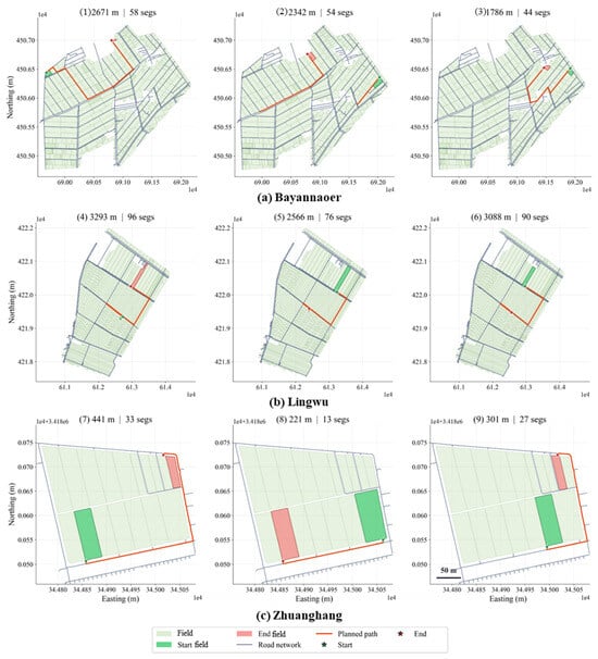
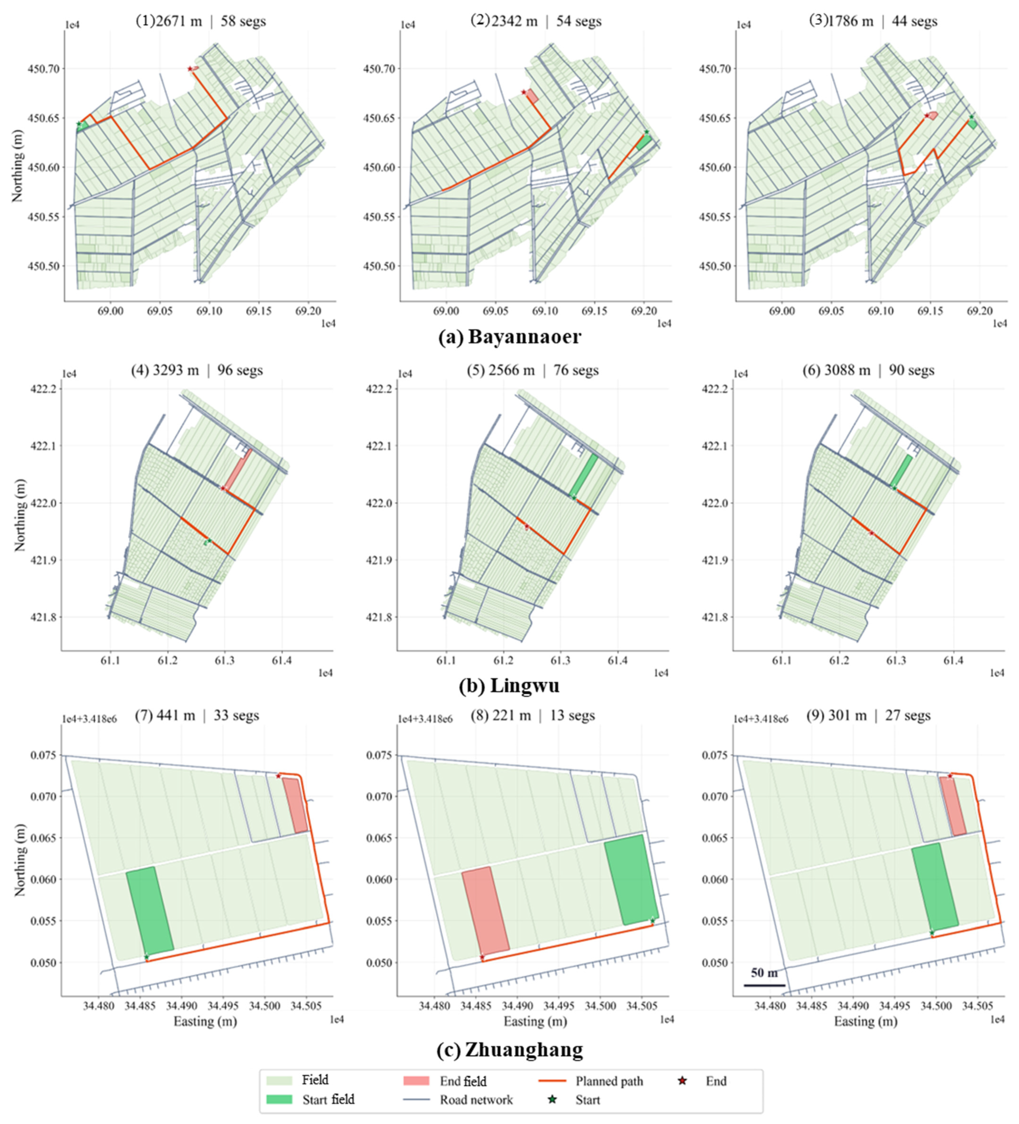
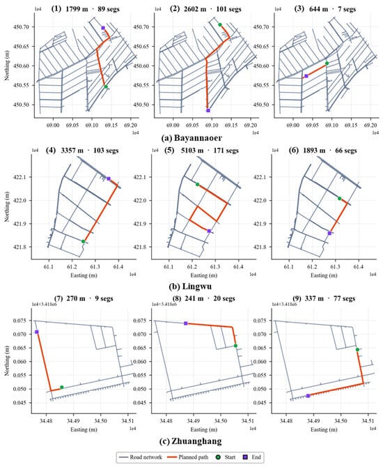
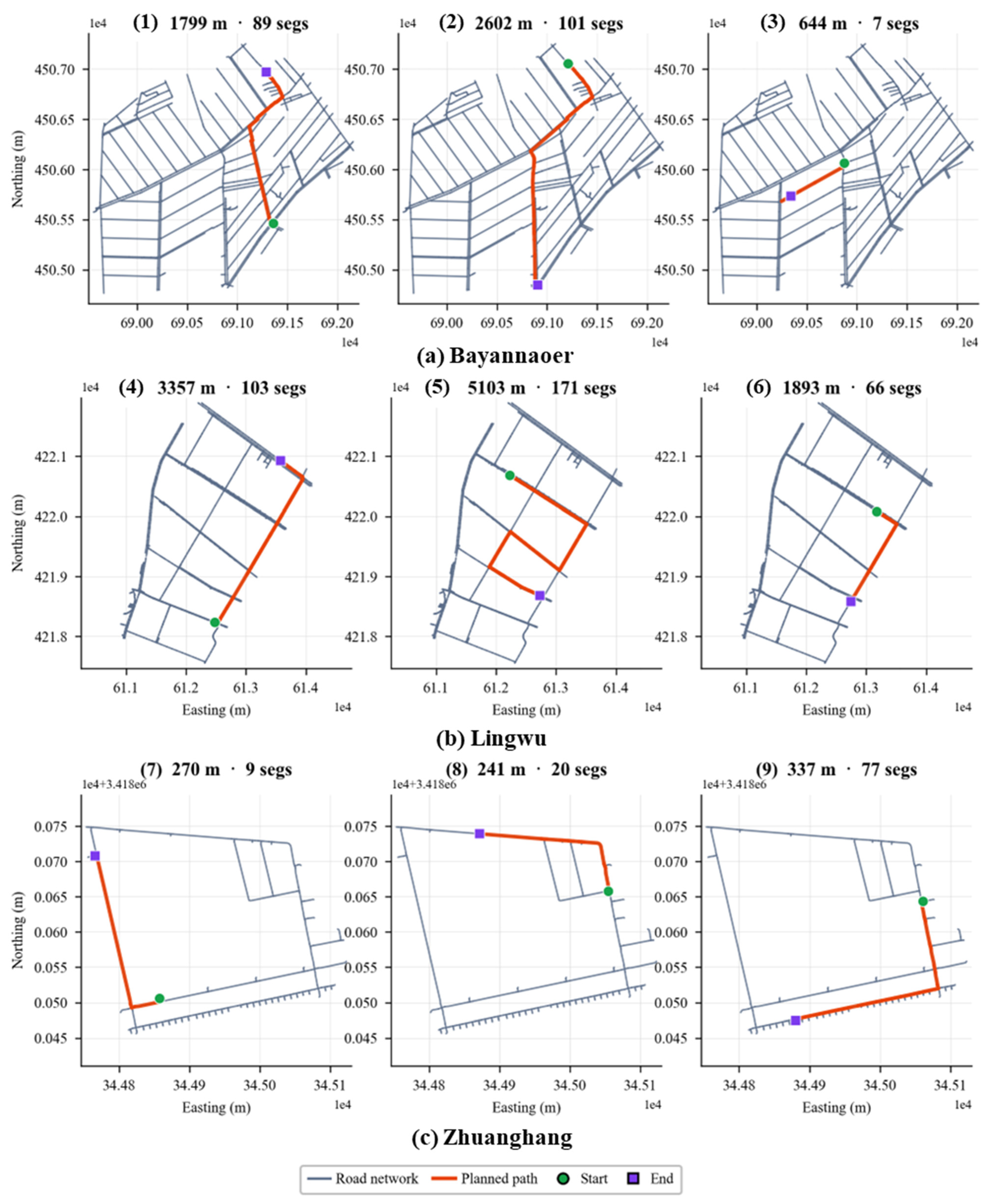
Figure 14 presents path-planning examples involving field parcels. Continuous paths are obtained for field-to-road, road-to-field, and field-to-field tasks, indicating that the bidirectional road–field-parcel mapping can be consumed directly by the planner. Figure 15 shows network-level examples: paths are found in all three study sites, and route patterns are consistent with local connectivity, suggesting that the topological data support batch solving across different network scales.

Figure 14. Multi-scenario path-planning results involving field parcels in the three study areas. Each panel shows the road network, start and end fields, and the planned route, with path length and segment count for field-access-related tasks.

Figure 15. Network-level path-planning results on the constructed topological graphs in three study areas. Each panel shows the road network, start and end nodes, and the planned route, with path length and segment count.

Regarding efficiency, a single evaluation run takes 0.218 s, supporting offline batch testing. Overall, the constructed topological map supports all four task types with low per-run computational cost, while high-error cases concentrate near intersections and field access points.

4. Discussion

4.1. Navigation Application Value of Farm-Road Topological-Map Construction

This study focuses on constructing farm-road topological maps from road and field vector data to support autonomous agricultural machinery operation in unmanned farms. Unlike methods that extract road centerlines only as geometric objects, the proposed method transforms road polygons and farmland parcels into a structured road-network representation that integrates centerline geometry, node–edge connectivity, road segment-width attributes, and bidirectional road–field links.

The experimental results show that the constructed maps can support navigation-related tasks such as path planning and operation scheduling. Compared with the skeletonization methods used for comparison, the proposed method achieved lower centerline errors and showed more balanced performance in both the Pred→GT and GT→Pred directions. This indicates that the extracted centerlines were not only closer to the reference centerlines, but also provided better coverage of the reference road network.

4.2. Effects of Road Ends and Intersections on Topology Construction

Road ends and intersections are key regions that affect the quality of farm-road topology construction. Many farm roads have irregular terminal shapes, flat-cut road ends, or abrupt changes in road width. If these local geometries are skeletonized directly, short spurs, shifted endpoints, or unstable branch directions may be generated. Such errors may affect node positioning and graph construction after centerline extraction, reducing the reliability of the resulting topological map.

Road-end filleting reduces this problem by smoothing terminal road boundaries before skeleton extraction. This helps the skeleton converge to a stable endpoint and reduces the possibility of generating multiple competing terminal branches. Similarly, intersection-area modeling improves the conversion from raster skeletons to node–edge graphs. In raw skeletons, complex intersections are often represented as clusters of high-degree pixels rather than as a single stable node. If these pixels are traced directly, redundant short segments and duplicated nodes may appear. By defining intersection areas and reconstructing local connections using clipping points, the proposed method can generate a clearer node–edge structure and improve the consistency of segment partitioning at intersections.

4.3. Relationships Among Centerline Geometry, Width Estimation, and Path Planning

The results also show that centerline geometry affects subsequent road-width estimation. In this study, road width was estimated by constructing normal cross-sections along segment centerlines and intersecting them with road-polygon boundaries. Therefore, the accuracy of width estimation depends not only on the road boundary, but also on the local direction of the centerline. When the centerline contains zigzags or local offsets, the normal direction may deviate from the true road cross-section direction, leading to biased or abnormal width samples. This explains why centerline smoothing remains useful even when the improvement in centerline positional accuracy is not obvious: smoothing stabilizes the tangent and normal directions used for width sampling.

Path-planning results further indicate that the navigation performance of the constructed map depends on both geometric and topological correctness. Even when centerline errors are small, incorrect graph connectivity, segment partitioning, or road–field association can still lead to inappropriate planned routes. Therefore, the large relative path-length errors observed in some cases should be interpreted in relation to local ambiguity in field-entrance association. When a target field is close to multiple candidate field-entrance nodes, small deviations in node position or road–field association may cause the route to enter the network through a neighboring road segment. Although the resulting route remains feasible, this local attachment difference can produce a large relative error, especially when the reference path is short. These results suggest that future evaluations of short field-entrance tasks should report both relative and absolute path-length errors.

4.4. Complementary Roles of the Main Processing Modules

The ablation results show that the main processing modules of the proposed method play complementary roles in the construction pipeline. Road-end filleting mainly improves terminal road geometry and corrects endpoint positions. Intersection-area modeling mainly improves node positions, road-skeleton positions, and local graph connectivity at complex intersections. Centerline smoothing mainly improves the stability of tangent estimation and width sampling. Therefore, these modules act on different error sources rather than jointly contributing to a single geometric correction.

This also explains why the full method outperformed the ablation variants in centerline extraction, width estimation, and path-planning evaluation. The workflow proposed in this study should be understood as a navigation-oriented topological-map construction pipeline rather than as a single skeletonization algorithm. Its value lies in integrating geometric preprocessing, skeleton extraction, node–edge graph construction, width assignment, and road–field association into a consistent representation for agricultural machinery navigation.

4.5. Applicability, Limitations, and Future Work

The proposed method is applicable to farms where road polygons and farmland parcels can be obtained from UAV orthoimagery, remote sensing, or manual vector annotation. Under these conditions, the method can transform two-dimensional road and field vector data into structured road-network data, thereby supporting path planning, operation scheduling, and machinery transfer between fields. This provides a practical spatial framework for autonomous agricultural machinery operating in farm environments.

Several limitations remain. First, the current map mainly represents road geometry and topology, but does not yet include operational passability factors. Machinery clearance, safety margins, road-surface condition, terrain slope, drainage ditches, temporary obstacles, and seasonal road changes may all affect whether agricultural machinery can safely pass through a road segment. Second, when field entrances, road ends, and parcel boundaries are close to one another, road–field association remains sensitive to local geometry. Third, complex intersections and highly irregular road boundaries may still produce local skeleton shifts or redundant branches, which can further propagate to graph construction and path-planning results.

Future work should further improve local topology construction around road ends, intersections, and field entrances. Entrance orientation and passability analysis of roads and field boundaries should be introduced to improve the geometric and topological accuracy of field-entrance nodes. In addition, the map should be extended from a geometrical–topological representation to an operation-oriented navigation representation by incorporating machinery-specific clearance and safety constraints. Broader validation on real agricultural machinery platforms is also needed to support practical deployment in unmanned farm operations.

5. Conclusions

This study proposed a method for constructing farm-road topological maps from road and field vector data to support agricultural machinery navigation in unmanned farms. By transforming road polygons and farmland parcels into a unified road-network representation, the method integrates centerline geometry, node–edge connectivity, road segment-width attributes, and bidirectional road–field links. The experimental results show that the proposed method can effectively generate structured farm-road topological maps, support navigation-related applications such as path planning and operation scheduling, and provide spatial infrastructure for full-process autonomous operation of agricultural machinery in farm environments.

Road ends, intersections, and field entrances remain the main sources of uncertainty in farm-road topology construction. Future work should improve local topology and passability modeling at these locations, incorporate operational constraints such as machinery clearance and terrain conditions, and validate the extended map on real agricultural platforms for unmanned farm deployment.

References

- National Bureau of Statistics of China. Statistical Communiqué of the People’s Republic of China on the 2024 National Economic and Social Development. Available online: https://www.stats.gov.cn/sj/zxfb/202502/t20250228_1958817.html (accessed on 19 June 2026). (In Chinese)
- Ding, H.; Zhang, B.; Zhou, J.; Yan, Y.; Tian, G.; Gu, B. Recent developments and applications of simultaneous localization and mapping in agriculture. J. Field Robot. 2022, 39, 956–983. [Google Scholar] [CrossRef] [Scilit]
- Lytridis, C.; Kaburlasos, V.G.; Pachidis, T.; Manios, M.; Vrochidou, E.; Kalampokas, T.; Chatzistamatis, S. An overview of cooperative robotics in agriculture. Agronomy 2021, 11, 1818. [Google Scholar] [CrossRef] [Scilit]
- Qu, J.; Zhang, Z.; Qin, Z.; Guo, K.; Li, D. Applications of autonomous navigation technologies for unmanned agricultural tractors: A review. Machines 2024, 12, 218. [Google Scholar] [CrossRef] [Scilit]
- Shao, S.; Xiao, L.; Lin, L.; Ren, C.; Tian, J. Road extraction convolutional neural network with embedded attention mechanism for remote sensing imagery. Remote Sens. 2022, 14, 2061. [Google Scholar] [CrossRef] [Scilit]
- Shao, Z.; Zhou, Z.; Huang, X.; Zhang, Y. MRENet: Simultaneous extraction of road surface and road centerline in complex urban scenes from very high-resolution images. Remote Sens. 2021, 13, 239. [Google Scholar] [CrossRef] [Scilit]
- Shi, M.; Feng, X.; Pan, S.; Song, X.; Jiang, L. A collaborative path planning method for intelligent agricultural machinery based on unmanned aerial vehicles. Electronics 2023, 12, 3232. [Google Scholar] [CrossRef] [Scilit]
- Wang, N.; Yang, X.; Wang, T.; Xiao, J.; Zhang, M.; Wang, H.; Li, H. Collaborative path planning and task allocation for multiple agricultural machines. Comput. Electron. Agric. 2023, 213, 108218. [Google Scholar] [CrossRef] [Scilit]
- Workman, R.; Wong, P.; Wright, A.; Wang, Z. Prediction of unpaved road conditions using high-resolution optical satellite imagery and machine learning. Remote Sens. 2023, 15, 3985. [Google Scholar] [CrossRef] [Scilit]
- Xiao, F.; Tong, L.; Li, Y.; Luo, S.; Benediktsson, J.A. A general spline-based method for centerline extraction from different segmented road maps in remote sensing imagery. Remote Sens. 2022, 14, 2074. [Google Scholar] [CrossRef] [Scilit]
- Yang, L.; Li, P.; Wang, T.; Miao, J.; Tian, J.; Chen, C.; Tan, J.; Wang, Z. Multi-area collision-free path planning and efficient task scheduling optimization for autonomous agricultural robots. Sci. Rep. 2024, 14, 18347. [Google Scholar] [CrossRef] [Scilit] [PubMed]
- Yang, M.; Yuan, Y.; Liu, G. SDUNet: Road extraction via spatial enhanced and densely connected UNet. Pattern Recognit. 2022, 126, 108549. [Google Scholar] [CrossRef] [Scilit]
- Yao, Z.; Zhao, C.; Zhang, T. Agricultural machinery automatic navigation technology. iScience 2024, 27, 108714. [Google Scholar] [CrossRef] [Scilit] [PubMed]
- Cao, R.; Li, S.; Ji, Y.; Zhang, Z.; Xu, H.; Zhang, M.; Li, M.; Li, H. Task assignment of multiple agricultural machinery cooperation based on improved ant colony algorithm. Comput. Electron. Agric. 2021, 182, 105993. [Google Scholar] [CrossRef] [Scilit]
- Cao, R.; Guo, Y.; Zhang, Z.; Li, S.; Zhang, M.; Li, H.; Li, M. Global path conflict detection algorithm of multiple agricultural machinery cooperation based on topographic map and time window. Comput. Electron. Agric. 2023, 208, 107773. [Google Scholar] [CrossRef] [Scilit]
- Cordova-Cardenas, R.; Emmi, L.; Gonzalez-de-Santos, P. Enabling autonomous navigation on the farm: A mission planner for agricultural tasks. Agriculture 2023, 13, 2181. [Google Scholar] [CrossRef] [Scilit]
- Gao, R.; Zi, L.; Hu, L.; He, J.; Wang, P.; Huang, P.; Xie, J.; Liu, S. Methods and experiments of farm road layer construction and farm machinery transfer path planning. J. South China Agric. Univ. 2025, 46, 256–264. [Google Scholar] [CrossRef]
- Li, S.; Zhang, M.; Wang, N.; Cao, R.; Zhang, Z.; Ji, Y.; Li, H.; Wang, H. Intelligent scheduling method for multi-machine cooperative operation based on NSGA-III and improved ant colony algorithm. Comput. Electron. Agric. 2023, 204, 107532. [Google Scholar] [CrossRef] [Scilit]
- Zhang, C.; Jia, L.; Liu, S.; Dou, G.; Liu, Y.; Kong, B. Dynamic job allocation method of multiple agricultural machinery cooperation based on improved ant colony algorithm. Sci. Rep. 2024, 14, 22414. [Google Scholar] [CrossRef] [Scilit] [PubMed]
- Zhu, S.; Wang, B.; Pan, S.; Ye, Y.; Wang, E.; Mao, H. Task allocation of multi-machine collaborative operation for agricultural machinery based on the improved fireworks algorithm. Agronomy 2024, 14, 710. [Google Scholar] [CrossRef] [Scilit]
- Xu, Y.; Zhang, L.; Zhang, W.; Liu, S.; Li, J.; Li, X.; Wang, Y.; Li, Y. Fine-grained extraction of road networks via joint learning of connectivity and segmentation. arXiv 2023, arXiv:2312.04744. [Google Scholar]
- Duan, L.; Mapurisa, W.; Leras, M.; Lotter, L.; Tarabalka, Y. Brightearth roads: Towards fully automatic road network extraction from satellite imagery. arXiv 2024, arXiv:2406.14941. [Google Scholar]
- Cai, L.; Yin, Y.; Mao, Q.; Yang, J. Method of extracting intersection polygons based on centerline junctions. Sens. Mater. 2024, 36, 4441–4453. [Google Scholar] [CrossRef] [Scilit]
- Song, J.; Sun, Y.; Cai, Z.; Xiao, L.; Huang, Y.; Zheng, Y. URoadNet: Dual sparse attentive U-Net for multiscale road network extraction. arXiv 2024, arXiv:2412.17573. [Google Scholar]
- Haunert, J.-H.; Sester, M. Area collapse and road centerlines based on straight skeletons. GeoInformatica 2008, 12, 169–191. [Google Scholar]
- Wang, T.; Wang, G.; Tan, K.E. Holistically-nested structure-aware graph neural network for road extraction. arXiv 2024, arXiv:2407.02639. [Google Scholar]
- Chen, J.; Yang, L.; Wang, H.; Zhu, J.; Sun, G.; Dai, X.; Deng, M.; Shi, Y. Road extraction from high-resolution remote sensing images via local and global context reasoning. Remote Sens. 2023, 15, 4177. [Google Scholar] [CrossRef] [Scilit]
- Mahara, A.; Khan, M.R.K.; Rishe, N.D.; Wang, W.; Sadjadi, S.M. Automated road extraction from satellite imagery integrating dense depthwise dilated separable spatial pyramid pooling with DeepLabV3+. arXiv 2024, arXiv:2410.14836. [Google Scholar]
- Lourenço, M.; Estima, D.; Oliveira, H.; Oliveira, L.; Mora, A. Automatic rural road centerline detection and extraction from aerial images for a forest fire decision support system. Remote Sens. 2023, 15, 271. [Google Scholar] [CrossRef] [Scilit]
- Zhang, Z.; Zhao, Z.; Wang, D.; Wang, L. GraphMorph: Tubular structure extraction by morphing predicted graphs. arXiv 2025, arXiv:2502.11731. [Google Scholar]
- Deng, L.; Deng, Y.; Meng, Y.; Chen, J.; Xi, Z.; Liu, D.; Chu, Q. GLD-Road: A global-local decoding road network extraction model for remote sensing images. arXiv 2025, arXiv:2506.09553. [Google Scholar]
- Zhang, T.Y.; Suen, C.Y. A fast parallel algorithm for thinning digital patterns. Commun. ACM 1984, 27, 236–239. [Google Scholar] [CrossRef] [Scilit]
- Guo, Z.; Hall, R.W. Parallel thinning with two-subiteration algorithms. Commun. ACM 1989, 32, 359–373. [Google Scholar] [CrossRef] [Scilit]
- Blum, H. Biological shape and visual science. J. Theor. Biol. 1973, 38, 205–287. [Google Scholar] [CrossRef] [Scilit] [PubMed]
- Lee, D.T. Medial axis transformation of a planar shape. IEEE Trans. Pattern Anal. Mach. Intell. 1982, PAMI-4, 363–369. [Google Scholar] [CrossRef] [Scilit]
- Aurenhammer, F. Voronoi diagrams—A survey of a fundamental geometric data structure. ACM Comput. Surv. 1991, 23, 345–405. [Google Scholar] [CrossRef] [Scilit]
Disclaimer/Publisher’s Note: The statements, opinions and data contained in all publications are solely those of the individual author(s) and contributor(s) and not of MDPI and/or the editor(s). MDPI and/or the editor(s) disclaim responsibility for any injury to people or property resulting from any ideas, methods, instructions or products referred to in the content. |
© 2026 by the authors. Licensee MDPI, Basel, Switzerland. This article is an open access article distributed under the terms and conditions of the Creative Commons Attribution (CC BY) license.