


Highlights
What are the main findings?
- While global 25 m models exhibit remarkable topographic stability, they systematically underestimate mature canopies (>30 m) due to signal saturation; in contrast, high-resolution optical approaches like the 1 m photogrammetric PALS model (R2 = 0.74, RMSE = 4.89 m compared to ALS) and emerging deep learning architectures provide exceptional structural fidelity, though current out-of-the-box ML models require local calibration.
- Forest disturbance monitoring reveals a distinct performance trade-off: the vertically stable PALS model delivers the highest overall precision for identifying clear-cuts (F1 = 0.353, Precision = 0.52) but is conservative, detecting only 211.57 ha (50.99% of the reference area). It performed similarly to the ALS reference, which detected 187.66 ha (45.23%), whereas the global HRCH model captures a significantly larger overall spatial footprint of harvested areas, detecting 431.45 ha (103.9% of the reference area) despite its baseline height inaccuracies and DL model from Living Atlas performed slightly better than HRCH.
What are the implications of the main findings?
- High-resolution optical methods, specifically digital aerial photogrammetry and emerging deep learning architectures, can serve as cost-effective operational complements to LiDAR for continuously tracking forest dynamics, though deep learning currently requires local calibration to overcome systematic underestimation biases in mature stands.
- Despite specific vertical limitations, global canopy height models (CHMs) remain highly valuable, freely available tools for large-scale forest monitoring and carbon stock assessments in data-poor regions where expensive ALS data is unavailable.
Abstract
Accurate mapping of forest canopy height is fundamental to modern forestry, providing essential structural data for biomass estimation and monitoring forest health. This study evaluates the broad usability of global (25 m) and high-resolution (1 m) Canopy Height Models (CHMs) by comparing them against temporally aligned Airborne Laser Scanning (ALS) reference layers from 2018 and 2024. At the 25 m scale, we evaluated four global products: Global Forest Canopy Height (GFCH), Global Map of Tree Canopy Height (GMTCH), High-Resolution Canopy Height model of Earth (HRCH), and Europe Temporal Canopy Height (EUCH). These satellite-derived models exhibit significant height-dependent limitations, systematically underestimating mature forest canopies (>30 m) by more than 15 m due to signal saturation, though EUCH and GMTCH performed moderately better. Transitioning to 1 m high-resolution data revealed a dramatic recovery in structural fidelity. A photogrammetrically derived model (PALS) achieved an RMSE of 4.89 m and a Mean Error (ME) of 1.86 m, demonstrating remarkable vertical stability across complex topography, even on slopes >25°. While coniferous stands produced higher absolute errors (RMSE = 6.75 m) than deciduous stands (RMSE = 6.19 m) due to spire-like architectures, PALS effectively captured fine-scale canopy textures. Experimental deep learning architectures, specifically the ArcGIS Living Atlas model, showed promise with an RMSE of 8.90 m, though out-of-the-box implementations struggle without local calibration. For forest disturbance monitoring, a distinct performance trade-off emerged. High-resolution photogrammetry (PALS) provided the highest overall precision for identifying clear-cuts (F1 = 0.353) but was conservative, capturing only 51% of the reference area. In contrast, the global HRCH model captured the total spatial footprint (103.9% of area) despite its geometric inaccuracies. The Living Atlas deep learning model offered the most balanced sensitivity, detecting 118.6% of the area with a competitive F1 score of 0.326. Ultimately, digital aerial photogrammetry provides a cost-effective solution for frequent operational updates, such as the two-year national mapping cycle in the Czech Republic.
1. Introduction
In an era where global forest ecosystems face unprecedented threats from climate change and intensified human activities, the imperative for accurate, highly detailed, and frequently updated information on forest structure has positioned advanced remote sensing technologies at the very forefront of forest monitoring and research. While conventional forest assessments remain foundational, LiDAR (Light Detection and Ranging) and the derived Canopy Height Models (CHMs) are increasingly preferred in modern forestry for their ability to deliver a more comprehensive and efficient understanding of forest characteristics. As an active remote sensing, LiDAR enables the acquisition of detailed vertical structure of trees and accurate measurements of canopy height [1,2]. Nowadays, CHMs offer unprecedented detail and accuracy, which can be used in many applications ranging from biomass and volume estimations, primary production, and forest damage assessment to efficient planning of harvesting [3,4,5,6,7,8]. Given the severe pressures on global forest ecosystems due to climate change and anthropogenic impact, the continuous, high-resolution mapping of forest height has become a priority for satellite observations [9].
Traditionally, the assessment of standing tree height has relied on conventional field methods, either through direct measurement (e.g., climbing trees, measuring fallen trees, or using telescopic poles) or indirect techniques (such as hypsometers or rangefinders). A very common method is combining visual estimation of treetops with trigonometric calculations. Additionally, other techniques are based on physical model inversions derived from field-measured data. However, these methods tend to be very time-consuming, costly, and impractical for large-area coverage [10]. Temporal resolution is also challenging since repeated field campaigns are logistically difficult, resource-intensive, and highly dependent on personnel and weather conditions. In contrast, remote sensing provides a relatively fast and cost-effective way to gather large amounts of data across different spatial and temporal scales [11].
The ability to accurately and rapidly detect forest clearings is paramount for effective forest management, monitoring deforestation, detecting illegal logging, and also understanding changes in land-use dynamics. While optical remote sensing has been a long-time primary tool for this application, satellite and airborne LiDAR can offer a unique advantage for robust and precise clearing detection [12,13].
Recent developments in spaceborne LiDAR technology have completely changed how we estimate forest canopy height and create global products. Following the pioneering but limited single-point measurements from the first ICESat mission, a new generation of sophisticated sensors has provided an unprecedented wealth of data, significantly improving our ability to map and monitor forest structures from space [14]. Two missions, in particular, have a key role in this topic: NASA’s ICESat-2 and the Global Ecosystem Dynamics Investigation (GEDI). Launched in 2018, ICESat-2 uses a photon-counting lidar system that enables it to measure individual photons. This innovation provides a high-density set of height measurements, enabling a much more detailed and precise mapping of vegetation structure. Similarly, GEDI, mounted on the International Space Station, uses a full-waveform LiDAR system to capture detailed vertical profiles of forest canopies. Its high-power laser beams provide millions of measurements across the globe’s tropical and temperate forests [15].
Recent developments in machine learning possibilities have also accelerated this topic. While missions like GEDI and ICESat-2 provide highly accurate height measurements, they are essentially point samples rather than continuous maps. Machine learning models can bridge this gap by learning the complex relationship between sparse lidar measurements and readily available wall-to-wall satellite imagery from sources such as Sentinel-1, Sentinel-2, or Landsat. Using Random Forest, gradient boosting, or deep learning neural networks with spaceborne LiDAR data, multispectral or radar imagery, it is now possible to create highly accurate, continuous maps of forest canopy height [16,17].
Beyond broad-scale mapping, ALS data have proven invaluable as highly effective training data for generating more localized and very high-resolution CHMs, often at sub-meter scales. For instance, at a national scale [18] leveraged airborne LiDAR to train gradient-boosted regression trees using 3.7 m Planet Dove imagery, enabling the generation of biomass maps across Peru, albeit with higher uncertainties in transitional and land-use change hotspot areas. More recently, Europe saw the computation of a 3 m CHM by [19], who employed 3 m Planet imagery and trained two U-Nets to predict tree extent and CHM, using both LiDAR observations and existing CHM predictions for training. Further pushing the resolution boundaries [20], successfully generated a sub-meter CHM for California, USA, by training a regression U-Net CNN on 60 cm imagery from the USDA-NAIP program, incorporating aerial LiDAR as the crucial training dataset.
Despite these examples of high-resolution, locally trained CHMs derived from aerial LiDAR, most countries lack the extensive, high-cost data needed to create them. This is where global canopy height models become essential [21]. These global models, while often coarser than their localized counterparts, bridge this data gap by providing a standardized, consistent, and freely available dataset for regions where no local alternative exists. It enables large-scale forest monitoring, biomass estimation, and carbon stock assessments in data-poor countries, bridging a critical information gap for climate and environmental science. For these countries, the further development of global CHMs is crucial for informed land management and climate-change mitigation strategies. It is therefore equally important to thoroughly test the accuracy and reliability of these global models to ensure their effective and trustworthy application [22].
Since the cost and power requirements limit how much of Earth can be covered by LiDAR, there is a push to explore other remote sensing methods. These include different approaches to laser scanning, such as terrestrial or mobile (TLS, MLS), multispectral satellite imagery, and radar remote sensing. A viable alternative is digital aerial photogrammetry (DAP), mainly because it provides 3D point clouds at lower costs and with acceptable accuracy compared to ALS [23,24,25].
In this study, we (1) evaluated the vertical accuracy of 4 global canopy height models and a photogrammetrically derived PALS model using airborne laser scanning (ALS) reference data in the University Forest Enterprise Masaryk Forest in Křtiny, Czech Republic; (2) assessed the influence of canopy height, terrain complexity and forest composition as sources of error in both 25 m and 1 m resolution models; (3) and assessed the usability of global canopy height models, ALS, and photogrammetry for the accurate detection and mapping of forest clear-cuts. Finally, we (4) evaluated the potential of deep learning architectures to improve fine-scale canopy height estimation compared to the ALS reference.
2. Materials and Methods
2.1. Study Area
Our study focuses on detecting forest clearings within the University Forest Enterprise Masaryk Forest in Křtiny (UFE Křtiny), a continuous forest complex of approximately 10,200 hectares located just north of Brno, Czech Republic (Figure 1). This area is ideal for our research due to its active management and diverse regeneration practices, including logging-related clearings.
Figure 1.
Location and extent of the study area. The inset map shows the position of the study area within the Czech Republic, with black lines indicating regional boundaries. The map pin marks the location of UFE Křtiny. In the orthophoto, the yellow line indicates the approximate study area extent, corresponding to the spatial coverage of the processed UFE Křtiny data.
The forests exhibit varied habitat conditions, with a 62:38 deciduous-to-coniferous species ratio, where beech, spruce, oak, larch, and pine dominate, resulting in complex canopy structures. Furthermore, a significant portion of the area falls within protected categories like the Moravian Karst Protected Landscape Area (29%) and NATURA 2000 sites (44%), making it a compelling case study for observing how clearings manifest across different management regimes and conservation statuses.
2.2. Reference ALS Data
As a reference for the tested models, we used ALS data acquired during the summer airborne campaign over the Masaryk Forest Training Forest area on 13 August 2024, as well as from 2018. The data acquisition, lasting approximately 200 min, was performed under favorable atmospheric conditions with no low, middle, or high cloud cover and a relatively high solar elevation angle of 40°. The acquired point cloud was classified into ground and non-ground points, and then further processed into GeoTIFF format for Digital Terrain Model (DTM), Digital Surface Model (DSM), and Canopy Height Model (CHM) rasters. The airborne campaign and initial processing were performed by the Department of Airborne Activities in the Global Change Research Institute CAS (Czechglobe). Parameters of the used laser scanner are highlighted in Table 1.
Table 1.
Parameters of reference ALS sensor.
2.3. Airborne Photogrammetric Data
In this study, we also utilized the Digital Surface Model generated by image correlation (DMP OK). This high-resolution DSM, developed by the Czech Office for Surveying, Mapping, and Cadastre (ČÚZK), represents the next-generation surface model derived from image correlation techniques, intended to replace the earlier DMP 1G model based on airborne laser scanning [26]. As of autumn 2025, DMP OK has been released for the Eastern zone of the Czech Republic, with full national coverage expected by mid-2026. Detailed parameters of individual aerial sensors are described in Table 2. The dataset provides elevation data in a classified format (las/laz), distinguishing terrain, buildings, and vegetation. It is georeferenced in the S-JTSK coordinate system and Baltic 1957 height vertical datum, ensuring compatibility with national geospatial standards. DMP OK will offer improved update frequency and accuracy compared to its predecessor, making it suitable for applications that require detailed surface representation, such as forest structure analysis, forest modeling, and landscape-level ecological assessment. In the future, the model is expected to be updated every two years, providing new data in alignment with the update cycle of the orthophoto map. The ALS-derived canopy height model is visualized at 25 m resolution in Figure 2 and at its native 1 m resolution in Figure 3 to serve as the primary reference for vertical accuracy.
Table 2.
Parameters of sensors used by ČÚZK for aerial survey photogrammetry.
Figure 2.
Spatial distribution and structural characteristics of the evaluated CHMs at 25 m resolution. The top row shows the height distribution across the full study area; the middle row provides detailed subsets of the region highlighted by the red rectangle; and the bottom row presents the corresponding height frequency distributions for each model.
Figure 3.
Spatial distribution and structural characteristics of canopy height for the high-resolution HRCH model, ALS reference data, photogrammetric CHM model (PALS) at 1 m resolution (top row), the middle row provides a detailed subset of the region highlighted by the red rectangle; and the bottom row presents the corresponding height frequency distributions for each model.
2.4. Tested Global Canopy Height Models
2.4.1. Global Forest Canopy Height Map (GFCH)
A global forest canopy height dataset for the year 2019 was developed by [27], featuring a 30 m spatial resolution. This dataset was developed by integrating Global Ecosystem Dynamics Investigation (GEDI) lidar forest structure measurements with Landsat time-series data (Figure 2). GEDI provides measurements of vegetation structure, including forest canopy height, between 52°N and 52°S on a global scale. They used Landsat multitemporal metrics (https://glad.geog.umd.edu/ard/home, accessed on 10 January 2026), which were supplemented by land surface elevation calculated from the Shuttle Radar Topography Mission (SRTM). Both datasets were imported into a regression tree algorithm to extrapolate GEDI Collection 1 canopy height values acquired between April and October 2019. To calibrate the model, the authors used the GEDI RH95 metric, which corresponds to the 95th percentile of energy return height relative to the ground as the estimate of canopy top height. The use of locally calibrated moving windows ensured high-quality forest height prediction and better consistency on a global scale. In areas beyond the GLAD data range, the model was extrapolated to produce the global forest map. Collection 2 data with improved geolocation accuracy is now available [28,29].
2.4.2. ETH Global Sentinel-2 10 m Canopy Height (GMTCH)
In a study by [30], the first global canopy height map at 10 m spatial resolution for the year 2020 was presented (https://langnico.github.io/globalcanopyheight/, accessed on 10 January 2026). The dataset is visualized in Figure 2. To achieve a better resolution, the authors combined GEDI lidar data with dense Sentinel-2 imagery using a deep learning model. Using convolutional neural networks (CNN), the authors fused GEDI data from 2019 to 2020 with cloud-free Sentinel-2 imagery to generate a dense, high-resolution canopy height map. Authors were able to transform GEDI images acquired between April and August of both 2019 and 2020 with Sentinel-2 images of the lowest cloud coverage between May and September 2020, into a dense canopy height map at the same spatial resolution with the help of convolutional neural networks (CNN). Using this approach enables globally consistent estimation of canopy height and its associated uncertainties at a 10 m ground sampling distance. It also reduces the common saturation effect in satellite-based height estimation, improving the detection of tall canopies that typically store large amounts of carbon.
2.4.3. High Resolution 1 m Global Canopy Height Map (HRCH)
The first global canopy height dataset of approximately 1 m resolution was created through a collaboration between Meta and the World Resources Institute [31]. The dataset is visualized at a 25 m spatial resolution in Figure 2, while Figure 3 presents the same dataset at its native resolution of approximately 1 m. The map was created using these steps: (1) the extraction of features from a self-supervised model trained on high-resolution (~1 m) imagery from WorldView-2, WorldView-3, and Quickbird II satellites, covering the years 2009 through 2020 (80% of the imagery is from the 2018 to 2020 period). The imagery consisted of 18 million “cloud free” satellite images of red, green, and blue (RGB) bands, with approximately 0.5 m resolution, from across the globe; (2) supervised training of a dense prediction decoder using pairs of ALS CHM and RGB satellite images; and (3) postprocessing using a convolutional network trained on 13 million GEDI observations to correct a potential bias coming from a geographically limited source of supervision [31]. To create this dataset, engineers used a state-of-the-art AI model, DiNOv2, based on methods developed by Meta Research’s AI team. The model was trained on 18 million satellite images.
2.4.4. Europe Temporal Canopy Height (EUCH)
In 2025, a new 10 m high-resolution canopy height model for Europe will be developed (Figure 2). Authors [32] trained and modified a 3D U-Net architecture design to extract both spatial and temporal features from multi-source satellite data. The model’s input consists of a 12-month stack of Sentinel-2 multispectral images concatenated with an annual median composite of Sentinel-1 radar data. For training, the authors used sparse GEDI LiDAR measurements (rh98 metric) as the ground truth. The final model, referred to as 3D-STACK-MULTIYEAR, was trained on a massive dataset of 800,000 patches covering the European continent. To ensure temporal consistency and reduce noise from fluctuating predictions, they applied a quadratic smoothing spline as a post-processing step to the resulting maps.
2.5. Generation of CHM Model Using Photogrammetric DSM
To compare the usability of photogrammetry in forest canopy height estimation, another CHM model (PALS) was generated by subtracting a photogrammetric Digital Surface Model (DMP OK) from a Digital Terrain Model (DTM) derived from ALS. We also had to address negative or invalid CHM values that may have arisen from model differences or terrain misalignment. A thresholding operation was performed using a SetNull condition to exclude all values below zero. This ensured that only meaningful canopy height values were retained for further analysis. The resulting photogrammetric CHM is presented at its native 1 m resolution (Figure 3) to illustrate the spatial consistency of the reconstructed canopy surface.
2.6. Generation of CHM Model Deep Learning Methods
In addition to comparing available global canopy height models, we tested the performance of high-resolution deep learning models for canopy height estimation. We used Meta’s canopy height architecture [31], a Vision Transformer (ViT) backbone (DINOv2) with a Dense Prediction Transformer (DPT) decoder, using two distinct deployment methods. First, we utilized the pre-trained “Deep Learning Model for Tree Canopy Height Estimation” hosted in ArcGIS Living Atlas (Esri; item ID: dac319ec70f844dab2d152f32dfff399; accessed on 10 January 2026). This model was trained on 0.5 m RGB imagery using self-supervised learning and fine-tuned with LiDAR data. We applied this model to photogrammetrically derived RGB orthomosaics from the PALS dataset at two spatial scales: 0.5 m and 1.0 m. This test aimed to evaluate the out-of-the-box performance of the model within a standard GIS ecosystem.
Secondly, we implemented the same architecture via the OpenGeoAI framework to allow for finer control over the inference process. For this method, we used the compressed_SSLhuge_aerial weights, specifically optimized for high-resolution aerial data, and restricted the input to the 1.0 m resolution orthomosaic. To maintain spatial consistency and prevent edge effects typical of deep learning on imagery, we employed a sliding-window tiling approach with a tile size of 256 × 256 pixels and an overlap set at 128 pixels. To smoothly transition between overlapping patches and eliminate boundary artifacts, the model used a raised-cosine window function. In Table 3 below is a summary of the key characteristics of the tested Canopy Height Models.
Table 3.
Parameters of tested CHM models.
2.7. Data Pre-Processing
To minimize temporal mismatch, each CHM product was compared with the ALS reference layer that best corresponded to the acquisition period or intended temporal representation of the product, rather than only to its nominal release year. GFCH, GMTCH, and EUCH were evaluated against the 2018 ALS reference layer, as these products represent forest conditions closer to the 2018–2020 period. HRCH was evaluated against the 2024 ALS reference layer because it was considered together with recent high-resolution products and disturbance-detection analyses; however, we explicitly acknowledge that its underlying Maxar imagery largely originates from 2018 to 2020. Therefore, the HRCH–ALS 2024 comparison may include both model-related error and real forest change between the image acquisition period and the ALS reference date.
Before the actual dataset analysis, all Canopy Height Model (CHM) datasets (GFCH, GMTCH, HRCH, EUCH, ALS, and PALS) underwent uniform spatial alignment. For the ALS-derived CHMs, circular zonal statistics were employed to extract maximum values within the target grid cells. Maximum values were used to preserve the upper canopy envelope and to avoid systematic lowering of canopy height that would occur if mean values were used. The ALS-derived CHMs were then resampled to 25 m resolution using bilinear interpolation for global model comparison and were also maintained at 1 m resolution for high-resolution assessment. Bilinear interpolation was selected for resampling continuous canopy-height rasters because canopy height represents a continuous surface and this method reduces abrupt transitions between neighboring cells. All remaining models were resampled to the native GFCH resolution, with pixels snapped to a common grid, and all datasets were reprojected to the UTM coordinate system.
Because the evaluated CHMs differ substantially in native spatial resolution, resampling was necessary to ensure pixel-to-pixel comparability. Nevertheless, this procedure may reduce local height extremes and smooth small canopy gaps, especially when high-resolution 1 m products are aggregated or resampled to coarser grids. Therefore, the reported inter-model differences should be interpreted as scale-dependent comparisons rather than as purely sensor-specific errors.
For the final statistical evaluation, a systematic point grid served as the basis for extracting local pixel values from each CHM. A 25 × 25 m grid was utilized for global product assessment, and for local, high-resolution models, we used a 10 × 10 m grid. From the dataset, we excluded outliers and processing artifacts, and several cleaning criteria were applied to the point dataset. Points with height values above 50 m or below 0 m were removed to maintain realistic forest structures. Additionally, we employed Ordinary Least Square (OLS) regression as a diagnostic filter: observations exhibiting a residual greater than 2.5 standard deviations from the mean were identified as statistical anomalies and excluded from the analysis. Lastly, for the PALS dataset, the Normalized Difference Vegetation Index (NDVI) was computed to identify and exclude shadowed areas (NDVI values between −0.5 and 0) from the point grid.
2.8. Statistical Accuracy Metrics
The vertical accuracy of the CHMs relative to the ALS reference was quantified using two primary statistical metrics: Mean Error (ME) and Root Mean Square Error (RMSE). ME was used to identify the presence and direction of systematic bias, where a negative value confirms an underestimation of canopy height. The RMSE provides a comprehensive measure of total error, combining both systematic bias and random variability. These metrics were calculated as follows:
where hi is the canopy height from tested global canopy height models, hREFi is the reference height from ALS, and n is the number of samples.
2.9. Influence of Canopy Height, Terrain Slope and Tree Species
In order to understand the factors influencing model accuracy, we analyzed model performance stratified by canopy height classes and terrain slope. The slope layer was derived from a Digital Terrain Model (DTM) created by the reference ALS dataset (it was generated at 1 m resolution and for the use case of 25 m model assessment was resampled). Model accuracy was assessed by grouping datasets into distinct canopy height classes. The point layer was partitioned into six classes based on the height values from the reference ALS CHM: 0–5 m, 5–10 m, 10–20 m, 20–30 m, 30–40 m, and >40 m. For each model within each height class, we assessed performance using the same key statistical metrics, ME and RMSE. ME was used to quantify the overall bias of the models, while RMSE provided a measure of overall accuracy.
We also wanted to test the influence of terrain complexity on model performance. Each model was additionally evaluated across slope intervals. Slope values were extracted for all grid cells and classified into five terrain categories: 0–5°, 5–10°, 10–15°, 15–20°, and >20°. Within each slope class, the same statistical metrics (ME, RMSE) were computed to quantify how model accuracy changes from flat terrain to increasingly steep slopes. This stratified analysis enabled a detailed examination of whether specific CHM models exhibit systematic increases in bias, reduced accuracy, or greater variability under more challenging topographic conditions. Finally, to evaluate the reliability of global CHMs, we assessed their accuracy using field-measured reference points from the Forest Management Plan of the University Forest Enterprise (UFE) at Mendel University. These points served as our ground truth and were filtered to include only stands with high homogeneity (where the dominant species accounts for more than 70% of the occurrence). The final validation dataset consisted of 363 coniferous sites and 490 deciduous sites. Performance across these sites was quantified using statistical metrics ME and RMSE.
2.10. Forest Clearcuts Detection
Beyond vertical accuracy assessment, this study evaluated the usability of CHMs for forest disturbance mapping, with clear-cut detection selected as the main operational use case. The workflow was designed as a rule-based structural diagnostic approach rather than as a supervised classification model. Therefore, no training samples were used. Instead, the method relied on canopy-height information derived directly from each CHM.
To harmonize models with different native resolutions (1 m, 10 m, and 25 m), all products were analyzed within a standardized 25 m spatial framework. The Global Forest Watch (GFW) Forest Loss layer was used as an external temporal benchmark for evaluating the CHM-derived clear-cut layers. To improve temporal consistency, model-specific GFW loss layers were generated according to the acquisition period or temporal representation of the evaluated CHM product. For example, the ALS 2024 model was compared with a cumulative GFW layer representing total forest loss from 2001 through 2024.
The classification process preserved the native resolution of each input CHM as far as possible. Each CHM was first reclassified into a binary low-canopy mask, where pixels below 2 m were designated as potential clearings or areas with strongly reduced canopy cover. The 2 m threshold was selected to minimize the influence of ground-level noise and very low vegetation while still capturing recent clear-cuts and early regeneration stages. The same threshold was applied to all CHM products to ensure a standardized comparison of their disturbance-detection behavior. However, because the tested products differ in spatial resolution and systematic bias, this threshold should be interpreted as a diagnostic criterion rather than as an optimized model-specific classification threshold.
To resolve differences between 1 m, 10 m, and 25 m datasets, the binary low-canopy masks were aggregated into a common 25 m grid, aligned with the GEDI footprint scale. For each 25 m cell, zonal statistics were used to calculate the proportion of pixels below the 2 m threshold. This fraction was interpreted as a scale-independent proxy for canopy openness or “canopy emptiness”, allowing a consistent comparison of clearing density across sensors regardless of their original spatial detail. The resulting 25 m disturbance rasters were then compared with the temporally synchronized GFW benchmark.
The performance of the clear-cut detection workflow was evaluated using a confusion-matrix-based approach. Precision, recall, and F1 score were used as the primary evaluation metrics. Precision quantified the proportion of CHM-detected disturbance cells that coincided with the GFW forest-loss layer, whereas recall quantified the proportion of GFW forest-loss cells captured by the CHM-based workflow. The F1 score, calculated as the harmonic mean of precision and recall, was used to summarize the balance between omission and commission errors. In addition, the total detected area and its percentage relative to the GFW reference area were reported as supplementary indicators of spatial coverage, but they were not interpreted as standalone measures of classification accuracy.
3. Results
3.1. Comparison of Global CHM Models at 25 m Resolution
3.1.1. Overall Accuracy
The comparison of global CHMs against the reference ALS model at a 25 m resolution revealed varying degrees of reliability among the tested models, as summarized in Table 4. While the reference ALS models from 2018 and 2024 covered canopy height ranging from near-ground level to approximately 50 m, the global CHMs demonstrated significant underestimation. The global models GFCH, GMTCH, and HRCH all failed to capture the upper limit of canopy height, with maximum predicted heights of 32, 39, and 30 m, respectively, despite the reference ALS reaching 50 m. The 2019 EUCH model was the only satellite product to capture a more realistic maximum height of 51.49 m. Every model showed a negative Mean Error (ME), indicating a consistent underestimation of canopy height at the 25 m scale. HRCH exhibited the most severe bias with an ME of −14.35 m, followed by GFCH, GMTCH, and EUCH, with values ranging from −4.98 to −3.11 m. This disparity was further supported by RMSE results; while EUCH (RMSE = 7.27 m) and GMTCH (RMSE = 7.61 m) had relatively moderate errors, GFCH performed significantly worse (RMSE = 9.88 m). The HRCH model displayed the highest error at 15.89 m, nearly twice that of the best-performing models. The highest relative stability in the taller canopy was found in the EUCH model, though it suffers from higher variability (SD = 7.25 m) compared to other CHM models.
Table 4.
Statistical summary of height distributions and vertical error estimates for 25 m global CHM models.
3.1.2. Influence of Canopy Height, Slope and Tree Species on Model Accuracy
Building on the previous point-to-point validation, performance was further stratified by canopy height to identify specific patterns of bias across different forest structures. The error distribution in Figure 4 revealed that the global models exhibited a significant transition in bias. In the lowest height class (0–10 m), GFCH and GMTCH show substantial overestimation with ME of 9.65 and 10.7 m, respectively, while HRCH is the only model to show underestimation (ME = −6.18 m). As canopy height increases beyond 20 m, all global models shift toward systematic underestimation. This trend is most pronounced in the tallest stands (40–50 m), where HRCH displays the most severe bias (ME = −24.9 m), followed by GFCH (−18.62 m) and GMTCH (−14.09 m).
Figure 4.
Distribution of vertical errors across canopy height classes for the 25 m resolution CHM models. The dashed vertical line at zero represents perfect agreement with the ALS reference.
The analysis of terrain complexity influence in Figure 5 indicates that topographic steepness significantly impacts the reliability of specific models. The accuracy of EUCH slightly improved as the terrain became steeper; its negative bias of −3.9 m on flat terrain improved to −0.8 m on steep slopes (>25°), accompanied by a decrease in RMSE from 7.38 to 6.58. The GFCH model showed the opposite performance, with the highest sensitivity to terrain and deteriorating performance as the slope increases (ME widened from −4.11 to −6.66 m). Both GMTCH and HRCH displayed consistent error profiles across the slope gradient. GMTCH stayed within a narrow range (−3.17 to −3.49 m ME), while HRCH consistently displayed the most significant underestimation, with ME ranging from −13.48 to −14.97 m.
Figure 5.
Distribution of vertical errors across terrain slope classes for the 25 m resolution CHM models. The dashed vertical line at zero represents perfect agreement with the ALS reference.
The model accuracy analysis was expanded to assess the role of vegetation type, specifically comparing performance within coniferous and deciduous forest stands. This stratification highlights a systematic disparity in error magnitudes, with all models exhibiting significantly higher precision in deciduous environments.
In coniferous environments, satellite-derived models saw a marked degradation: HRCH recorded its most severe underestimation (ME = −15.04 m; RMSE = 18.06 m), and GFCH followed with an RMSE of 13.52 m. EUCH and GMTCH likewise showed increased variability and deeper negative biases when transitioning from deciduous to coniferous cover. As visualized in the absolute error distributions (Figure 6), coniferous stands consistently produce a broader range of high-magnitude outliers, whereas deciduous forests allow for more concentrated error profiles with lower overall variance. Figure 7 further confirms these results by highlighting that models struggle to reach the full height of mature coniferous stands, tending to smooth over individual tree crown peaks.
Figure 6.
Distribution of absolute vertical errors stratified by forest composition for the 25 m resolution CHM models.
Figure 7.
Canopy height profiles of the evaluated 25 m CHM products compared with the ALS reference along three selected transects. Each transect consists of an orthophoto overview with the profile line shown in red and the corresponding canopy-height profile below. The profiles illustrate differences in canopy-height representation across heterogeneous forest stands, canopy gaps, and varying topographical gradients. The gray point cloud represents the ALS reference, while colored lines represent the evaluated CHM products. Vertical dashed red lines indicate selected disturbance or transition zones along the transects.
In Figure 7, it is further noticeable that global models (especially GFCH and GMTCH) consistently cut off the highest points of the canopy shown by the ALS. Unlike the high-frequency, jagged profile of the ALS data, the global models produce a flattened, simplified canopy envelope that ignores small-scale gaps and individual tree-crown variations. Of all the satellite products, EUCH (teal line) most frequently reaches the upper vertical limit of the forest stands, though it still “bridges” across gaps rather than dipping down to the ground.
3.2. Comparison of High-Resolution CHM Models at 1 m Resolution
The separate analysis of high-resolution models discovered a pattern that is fundamentally different from the 25 m model analysis. By utilizing a 1 m spatial resolution, the HRCH and PALS models successfully capture fine-scale canopy textures that were previously smoothed over, leading to a much more accurate alignment with the ALS reference data from 2024. The statistical summary in Table 5 demonstrates a significant reduction in the extreme vertical bias that was observed in the 25 m model analysis. PALS model maintained the highest level of precision (R2 = 0.74 and RMSE = 4.89 m). While it exhibits a slight systematic overestimation (ME = 1.86 m), it consistently tracks the absolute height of the reference canopy. The HRCH shows a dramatic recovery in accuracy; the severe underestimation bias of −14.35 m found in the 25 m version is reduced to −3.92 m at the 1 m scale. The 1 m models reach average heights (11.82–17.60 m) that are significantly closer to the ALS2024 reference mean of 15.74 m than any of the previously tested global models.
Table 5.
Comparison of high-resolution 1 m CHM model accuracy against the ALS reference.
The stratified canopy height analysis, visualized in Figure 8, highlights a foundational difference in how HRCH and PALS models capture canopy structure. The PALS model was exceptionally stable across all levels of canopy height. In lower canopies (0–10 m), the model shows slight overestimation with ME = 2.98 m and RMSE = 6.43 m. As height increases, the PALS model becomes significantly more precise, with near-perfect ME = 0.14 m and RMSE = 1.83 m. On the other hand, HRCH exhibits a sharp transition from slight overestimation to severe underestimation with growing canopy height. In the lowest parts of height classes (0–10 m), HRCH shows minor positive bias (ME = 1.01 m), but beyond 10 m, the models start to underestimate the canopy, failing to register the actual canopy height. ME shifts from −3.16 m in the 10–20 m class to a substantial −21.29 m in the tallest canopies (40–50 m). The RMSE also degrades significantly with height, ballooning from 6.83 m in young stands to 21.53 m in the tallest stands.
Figure 8.
Distribution of vertical errors across canopy height classes for the 1 m resolution CHM models. The dashed vertical line at zero represents perfect agreement with the ALS reference.
After analyzing the impact of terrain on the 1 m models, we found that both maintain high vertical stability even in complex terrain with steeper slopes. The PALS model exhibits remarkable consistency, with the Mean Error (ME) remaining nearly unchanged from flat terrain (0–5°: 1.93 m) to very steep slopes (>25°: 1.97 m). Its error distribution, as visualized in the ridge plots in Figure 9, remains tightly centered, indicating that its predictive reliability is largely unaffected by terrain complexity. Similarly, HRCH shows limited sensitivity to slope, with the RMSE increasing only slightly from 7.35 m on flat ground to 8.45 m on steep inclines. However, its broader distribution across all slope classes confirms that its vertical uncertainty is primarily driven by forest height rather than ground topography.
Figure 9.
Distribution of vertical errors across terrain slope classes for the 1 m resolution CHM models. The dashed vertical line at zero represents perfect agreement with the ALS reference.
The influence of forest composition revealed distinct behavioral patterns based on the canopy architecture and species-dependent structures (Figure 10). In coniferous stands, both models encountered higher absolute errors compared to deciduous stands. HRCH shows a lower systematic bias (ME = −1.12 m) than in deciduous zones, yet it suffers from high variability with a standard deviation (SD) of 8.05 m. The PALS model exhibits a higher RMSE (6.75 m) in conifers, which is likely attributed to the difficulty of capturing narrow, spire-like canopy peaks even at high spatial resolution. However, the performance in deciduous stands is generally more stable across both models. PALS achieves its lowest RMSE (6.19 m) in deciduous types, benefiting from the more continuous and hemispherical canopy surface, despite a higher systematic overestimation (ME = 2.28 m). The violin plots in Figure 10 confirm that error distributions are significantly more consolidated in deciduous types, whereas coniferous structures produce more extreme outliers and higher absolute error.
Figure 10.
Distribution of absolute vertical errors stratified by forest composition for the 1 m resolution CHM models.
The following analysis, using vertical profiles in Figure 11, provides a physical explanation for the statistical performance observed in the previous sections. In deciduous stands, the high-resolution models demonstrate their strongest structural fidelity; the PALS model tracks the complex “peaks and valleys” of the canopy surface with high precision, while HRCH follows the general trend but tends to smooth over the finer vertical details of individual crowns. This contrast becomes more pronounced in coniferous stands, where HRCH exhibits a severe systematic underestimation by failing to reach the upper canopy peaks, a gap that directly supports its higher ME compared to PALS. Conversely, the PALS model remains resilient in these structures, successfully identifying narrow coniferous spires and maintaining a much lower RMSE. At the boundaries of forest disturbances, such as clear-cuts, both models effectively respond to height changes, but with different sensitivities. PALS exhibits a sharp, near-instantaneous drop to ground level that perfectly captures the physical disturbance edge, whereas HRCH provides a more gradual response. This behavior illustrates why HRCH can achieve higher spatial recall in detection tasks; its broader, more “generous” estimation of canopy edges captures more area than the strict, pinpoint precision of the PALS model.
Figure 11.
Canopy height profiles of the evaluated 1 m resolution CHM products compared with the high-density ALS reference along three selected transects. Each transect consists of an orthophoto overview with the profile line shown in red and the corresponding canopy-height profile below. The profiles illustrate model performance across dense deciduous forest, fragmented forest stands, and structural disturbances such as clear-cuts. The gray point cloud represents the ALS reference, while the purple line indicates the ALS-derived canopy surface. Colored lines represent the evaluated high-resolution CHM products (HRCH, PALS). These profiles demonstrate the ability of 1 m products to capture fine-scale canopy peaks and gaps compared to the ALS benchmark.
3.3. Deep Learning Estimates of Canopy Height
To conclude our analysis, we evaluated the performance of deep learning architectures for canopy height estimation from RGB imagery. The ArcGIS Living Atlas model (DL_p100), despite its accessibility, exhibited a systematic overestimation with a ME of 1.84 m and a high RMSE of 8.90 m (Table 6). This lack of precision is visually evident in the spatial analysis (Figure 12), where the DL P100 output displays a “blocky” artifact and a fragmented canopy structure compared to the high-density ALS reference. Conversely, the OpenGeoAI implementation (DL_GeoAI) achieved a superior spatial correlation (R2 = 0.44), reflecting a better ability to map relative canopy patterns. However, this model suffered from a severe systematic underestimation bias of −8.89 m, resulting in a “plateau” effect where predicted heights were significantly lower than the true canopy peaks. The vertical profiles in Figure 13 further illustrate these behavioral signatures in dense forest. While the OpenGeoAI model maintains a smoother transition across the forest surface, it consistently sits several meters below the actual LiDAR-derived height cloud, whereas the ArcGIS model tracks closer to the mean height but fails to replicate the fine-scale structural variability of the mature stand.
Table 6.
Accuracy of the developed CHM models using deep learning algorithms evaluated against the ALS (2024) reference.
Figure 12.
Comparison between reference ALS CHM and two deep learning models: DL P100 (middle) and OpenGeoAI (bottom). The maps represent the same forested area in the Masaryk Forest, with a corresponding satellite image for visual context.
Figure 13.
Canopy height profiles for the evaluated 2 deep learning models (OpenGeoAI, DL P100) compared against the high-density ALS reference in a dense deciduous forest stand. Grey points represent individual height observations from the high-density ALS reference point cloud along the profile transect. The black line shows the ALS reference canopy height profile, while the blue and pink lines represent the OpenGeoAI and DL P100 model predictions, respectively.
3.4. Application of Tested Models—Detection of Clear-Cuts
The evaluation of a specific use case for tested canopy height models revealed a significant challenge in model performance. While a simple model comparison suggests only the PALS model demonstrated near-zero ME across all forest structures, the transition to a specific forestry application revealed a different outcome. Performance of all tested models is summarized in Table 7. The “near-zero” error of the PALS model in height points translated into a reliable Precision (User’s Accuracy = 0.52) and the highest F1 score (0.353) among the evaluated models for clear-cut detection. This confirms that a vertically stable model is the most trustworthy when it does signal a change. However, this stability came at the cost of being conservative; the PALS model detected 211.57 ha, mapping only 50.99% of the reference disturbances (Recall/PA = 0.27).
Table 7.
Accuracy of clear-cut detection across evaluated models. The reference area represents the GFW forest loss reference layer.
The significant transition in bias noted in the point-to-point validation, where GFCH, GMTCH, and EUCH swing from overestimating young forests to underestimating mature ones, rendered them effectively blind to clear-cuts. Their Recall (PA = 0) and minimal detected areas (38.46 ha for GFCH, 0.37 ha for GMTCH, and 0 ha with EUCH) indicate that their internal noise and height-stratified errors are larger than the signal of a forest being removed. Interestingly, although HRCH showed the worst systematic underestimation in tall forests (>25 m) and suffered from extremely low geometric accuracy (F1 = 0.013), it demonstrated exceptional sensitivity to disturbance. HRCH detected 431.45 ha, capturing 103.9% of the reference clear-cut area. This suggests a distinct performance trade-off. While its exact boundary delineation is poor, HRCH’s sensitivity to change effectively captures the broader spatial footprint of harvested areas. These results are visualized in Figure 9, where you can clearly see that HRCH and PALS are much more efficient at detecting forest clear-cuts, whereas the other global models are virtually absent from the map. The systematic canopy height underestimation observed in most global models creates a significant barrier to clear-cut detection. By failing to represent baseline forest height accurately, these models cannot reach the necessary height threshold to effectively map forest disturbance events like clear-cuts. The profile in a clear-cut section of the height profiles plot in Figure 14 further supports how global models struggle with forest disturbance mapping (except for the HRCH model).
Figure 14.
Spatial distribution of clear-cut detection using the tested canopy height models compared with the Global Forest Watch forest loss benchmark. The panels on the left show clear-cut detections derived from the tested CHM datasets. Different colors distinguish detections from individual models: EUCH, GFCH, HRCH, GMTCH, ALS, PALS, DL GeoAI, and DL P100. The panels on the right show the GFW forest loss benchmark, with red indicating forest loss detected during 2015–2020 and green indicating forest loss detected during 2020–2024. White lines represent the boundaries of the analyzed forest management units. The yellow rectangles in the overview insets indicate the detailed area shown in the main GFW panels.
The clear-cut detection results further indicate a distinct performance profile for the deep learning models. Using high-resolution RGB data, the deep learning architecture demonstrated a superior ability to capture the total extent of harvested areas compared to global models like GFCH. The ArcGIS Living Atlas model achieved a competitive F1-Score of 0.326 and detected 491.94 ha (118.57% of the reference area). The GeoAI model captured the largest overall footprint, detecting an extreme 1445.74 ha (348.45% of the reference), though its overprediction resulted in a lower F1-Score of 0.186. In contrast, the ALS maintained the highest precision (UA = 0.56) and an F1 score of 0.348, but its low recall (0.25) and detected area of only 187.66 ha (45.23%) suggested it missed a large portion of the overall footprint. Ultimately, the deep learning approaches capture a much broader area than the conservative ALS and PALS methods, though the relatively low overall F1 scores across all models highlight the persistent challenge of accurately delineating exact clear-cut boundaries using only height-based canopy data.
Analysis of the clear-cut detection results underlines significant variations in the performance profiles of the deep learning models. Using high-resolution RGB data, the deep learning architectures demonstrated a superior ability to capture the total extent of harvested areas compared to global satellite CHM models like GFCH. The ArcGIS Living Atlas model achieved a competitive F1-Score of 0.326 and detected 491.94 ha (118.57% of the reference area). The GeoAI model captured the largest overall footprint, detecting an extreme 1445.74 ha (348.45% of the reference), though its overprediction resulted in a lower F1-Score of 0.186. In contrast, the ALS reference method maintained the highest precision (UA = 0.56) and an F1 score of 0.348, but its low recall (0.25) and detected area of only 187.66 ha (45.23%) suggest it missed a large portion of the overall footprint. Ultimately, the deep learning approaches capture a much broader area than the conservative ALS and PALS methods, though the relatively low overall F1 scores across all models highlight the persistent challenge of accurately delineating exact, clear-cut boundaries using only height-based canopy data.
4. Discussion
With the arrival of a new generation of satellite sensors and advanced machine learning algorithms, Earth remote sensing is undergoing a revolution in its ability to monitor forest height. Whereas accurate mapping of vertical structure was previously the domain of costly aerial survey campaigns (ALS), global vegetation height models now make this data available on a continental to planetary scale. This study evaluated the potential of these new models and algorithms. Our results show that although global models represent a significant step forward, their use for precise monitoring faces specific limitations related to spatial and temporal resolution, signal saturation, and processing methodology.
4.1. Temporal Dynamics
A key challenge in validating multi-source CHM products is their temporal consistency. In this study, we attempted to minimize temporal mismatch by using two ALS reference layers. Models representing forest conditions around 2019–2020, namely GFCH, GMTCH, and EUCH, were compared with the 2018 ALS reference layer, whereas recent high-resolution products, including HRCH and PALS, were compared with the 2024 ALS reference layer. However, the nominal release year of a CHM product does not necessarily correspond to the acquisition period of its input imagery or training data. This is particularly relevant for HRCH, which was released as a recent high-resolution product but is largely based on Maxar imagery acquired between 2018 and 2020. Consequently, the comparison between HRCH and the 2024 ALS reference may partly reflect real forest growth, harvesting, or disturbance occurring between the image acquisition period and the ALS campaign, in addition to model-related errors.
This temporal issue was most evident for HRCH, which showed the strongest systematic underestimation among the evaluated global products, with ME = −14.35 m and RMSE = 15.89 m at 25 m resolution. This error pattern should be interpreted cautiously. It is likely related to a combination of temporal mismatch, model bias, spatial smoothing, and limitations in reconstructing tall canopy peaks, particularly in mature coniferous stands. By contrast, GFCH and GMTCH were compared with the 2018 ALS reference, which reduced temporal mismatch. Their remaining underestimation was therefore more likely associated with the limitations of coarse spatial resolution, GEDI–optical data fusion, signal saturation, and smoothing of the vertical canopy profile. Even when temporal mismatch is reduced, global models may encounter a height “ceiling” in mature stands and may be unable to fully distinguish height differences above approximately 30 m.
Temporal differences between products also influenced clear-cut detection. In some areas, HRCH may represent pre-disturbance canopy conditions, whereas PALS and ALS 2024 represent more recent post-disturbance conditions. This temporal contrast likely contributed to the relatively high spatial coverage and recall of HRCH in disturbance mapping. However, HRCH should not be interpreted as the most accurate clear-cut detection model overall. Although it detected a large disturbance extent, corresponding to 431.45 ha or 103.9% of the GFW reference area, its performance was characterized by a trade-off between sensitivity and precision. Specifically, HRCH achieved high recall but lower precision, resulting in a relatively low F1 score of 0.24. In contrast, PALS provided more conservative and spatially sharper clear-cut delineation, detecting 211.57 ha or 50.99% of the reference area, with higher precision and an F1 score of 0.353. This indicates that PALS agreed better with the GFW benchmark at the pixel level, whereas HRCH captured broader disturbance patterns but also included more false-positive areas.
These results demonstrate that vertical accuracy and disturbance-detection performance are not equivalent. A model with weaker absolute height accuracy may still be sensitive to broad canopy loss, while a vertically more accurate high-resolution model may produce more conservative disturbance boundaries. Therefore, CHM products should be selected according to the intended application: broad disturbance screening may benefit from higher recall, whereas operational clear-cut delineation requires higher precision and a stronger balance between precision and recall, as expressed by the F1 score.
The interpretation of clear-cut detection results is influenced by the selected reference benchmark. The GFW forest-loss layer provides a spatially consistent external reference, but it should not be considered error-free ground truth. GFW primarily detects spectral changes in canopy cover, whereas the CHM-based workflow identifies structural canopy removal or very low canopy height. Therefore, disagreement may occur in areas affected by bark beetle infestation, standing dead trees, partial canopy decline, early regeneration, shadow effects, or spatially complex stand edges. Precision, recall, and F1 score should therefore be interpreted as measures of agreement with the selected GFW benchmark rather than as absolute measures of clear-cut detection capability.
4.2. Influence of Environmental Factors on Model Accuracy
Our results indicate that stand height was one of the main factors associated with model error. A significant shift in the nature of the error was evident in the global GFCH and GMTCH models. In the youngest stands (0–10 m), these models systematically overestimate height (ME > 9 m). As stand height increases, the trend reverses toward asymptotic signal saturation. In mature stands (>30 m), the models reach their technological limit and fail to capture vertical growth. In mature stands (>30 m), the models appear to approach a saturation limit and show reduced ability to capture additional vertical variation. The most pronounced pattern was observed for HRCH, which underestimated canopy height in the 40–50 m class by nearly 25 m, indicating a substantial loss of information on the upper canopy layer. An important finding is that most models (with the exception of GFCH) are relatively immune to terrain slope. While GFCH’s accuracy decreases with increasing slope (ME worsens from −4.1 m to −6.7 m), the other models exhibit consistent errors regardless of topography. The EUCH model even shows a slight improvement in accuracy on steeper slopes, which may indicate that more modern data fusion algorithms are able to effectively compensate for the influence of terrain. Coniferous stands pose a greater challenge for 25 m models than deciduous ones. All tested models exhibited higher RMSE and more pronounced underestimation in coniferous stands. This supports the interpretation that, at coarse resolution, the narrow conical tips of spruce trees are smoothed out and blend into the surroundings, while the more compact crowns of deciduous trees are more easily detectable by satellite sensors.
The transition to 1 m resolution for the HRCH and PALS models resulted in a significant improvement in accuracy, but also revealed specific limitations related to the detailed crown architecture. The key difference between the PALS photogrammetric model and the model generated using AI reconstruction (HRCH) is stability across height classes. The PALS model showed comparatively stable vertical performance, with an error of nearly zero (0.2 m) regardless of whether it measures young stands or mature stands. In contrast, even at 1 m resolution, HRCH repeats the errors from the previous 25 m analysis. In low stands, the model is accurate, but in stands over 30 m, there is a sharp increase in error (ME up to −21.3 m). This suggests that, despite its finer nominal resolution, HRCH may still be limited by its training data, model architecture, or input imagery when reconstructing the full height of mature stands. Our analysis suggests that the error patterns in the 1 m models were more strongly associated with vegetation structure than with terrain slope. PALS exhibited identical accuracy on flat terrain and on slopes > 25 degrees. Our analysis confirmed that the error in the 1 m model is therefore primarily biological (stand type, vegetation height), not geomorphological. At a detailed scale, the limitations of the sensors also became fully apparent. In coniferous stands, the PALS model suffers from higher error rates (RMSE 6.75, compared to 6.19 m in deciduous stands). Photogrammetry may encounter difficulties in reconstructing sharp peaks and deep gaps in the canopy, which leads to various artifacts and the omission of tree tops. In deciduous stands, which form more continuous surfaces, both models are better able to capture stand height. HRCH fails more fundamentally in coniferous stands, not because of texture, but due to a systematic underestimation of total height.
4.3. Photogrammetry-Derived CHM Model
Although the PALS model, derived from digital aerial photogrammetry, demonstrated the highest degree of agreement with the reference ALS in our study (RMSE = 4.89 m; ME = 1.86 m), its validation at a native resolution of 1 m revealed specific artifacts inherent to the optical “image matching” method. Unlike laser scanning, which actively penetrates the forest structure, photogrammetry reconstructs only the visible surface. This leads to several phenomena that affect accuracy, particularly in coniferous stands. One of the most visible artifacts was a starburst-like pattern, observed mainly in coniferous stands. This phenomenon is likely related to the reconstruction of narrow conical spruce tips. Correlation algorithms (SGM—Semi-Global Matching) reach their limits when attempting to find corresponding points on the sharp tip of a tree from different viewing angles. Instead of precisely matching the tip, the algorithm tends to connect points in the immediate vicinity of the tip, thereby creating a star-shaped widening of the crown. This artifact may partly explain why the PALS model in our study exhibited a slight but systematic overestimation and why the error rate in coniferous stands (RMSE = 6.75 m) was higher than in deciduous stands (RMSE = 6.19 m). While the rounded crowns of deciduous trees form a continuous surface that is ideal for photogrammetry, the sharp geometries of conifers are artificially expanded, leading to a false increase in crown volume in the upper parts. These artifacts are visualized in Figure 15. Another key difference is penetration capability. PALS models the so-called canopy envelope. The photogrammetric point cloud describes only the outer layer that the camera “sees” and cannot penetrate small gaps in the canopy into the crown interior, as a laser beam can. As our elevation profiles show, PALS tends to bridge smaller gaps between branches, creating a smoother and more compact surface than the reference ALS. This is advantageous for estimating canopy closure, but it can lead to an underestimation of surface roughness and the overlooking of smaller windfalls or breaks that are hidden below the level of the surrounding canopy. Another key difference is penetration capability. PALS models the so-called canopy envelope. The photogrammetric point cloud describes only the outer layer that the camera “sees” and cannot penetrate small gaps in the canopy into the crown interior like a laser beam can. As our elevation profiles show, PALS tends to bridge smaller gaps between branches, creating a smoother and more compact surface than the reference ALS. This is advantageous for estimating canopy closure, but it can lead to an underestimation of surface roughness and the overlooking of smaller windfalls or breaks that are hidden below the level of the surrounding canopy. The quality of the PALS model is also highly dependent on lighting conditions and stand density. In heavily thinned or sparse stands, the method reaches the limits of the sensors’ dynamic range. The high contrast between the brightly lit canopy and the deep shadows in the ground gaps causes correlation algorithms to fail, as they cannot find sufficient texture in the shaded areas. The result is often a “shaky” surface model or data with high noise in the ground-level areas. However, our preprocessing steps reduced the influence of these problematic areas, although some residual uncertainty may remain. In terms of environmental influence, the PALS model showed high stability, compared with the tested global products. While satellite models encounter a saturation limit as stand height increases and systematically underestimate values in mature stands, photogrammetric data maintain consistent accuracy across the entire vertical profile. Our results show that the model error (RMSE) actually decreases with increasing tree height (from 6.43 m in young stands to 1.83 m in stands over 40 m), confirming high reliability for the inventory of mature stands. This robustness also applies to topography; thanks to surface normalization using a precise digital terrain model (DTM) from ALS, slope gradient had no effect on the results. Even in terrain with a slope exceeding 25°, the model achieved the same accuracy as on flat ground, confirming that the dominant source of uncertainty in photogrammetry is the texture of the canopy, not the geomorphology of the terrain. This level of stability, combined with the regular two-year cycle of aerial survey imagery in the Czech Republic, suggests a strong potential for large-scale operational use. Such a frequent update cycle allows for the transition from static ALS mapping to near-continuous monitoring of forest growth and vitality on a national level.
Figure 15.
The ALS model (left) shows a smooth, accurate forest canopy. In contrast, the PALS model (right) exhibits a noticeable starburst effect within the red circle. This artifact appears as jagged, radial noise and “speckled” gaps where the photogrammetric software failed to correctly match image points in dense or shadowed areas.
4.4. Deep Learning Potential for Accurate CHM Estimation
Our experiments with deep learning models (OpenGeoAI, Meta Living Atlas) have indicated that, although current “off-the-shelf” models suffer from systematic bias (e.g., OpenGeoAI underestimation of −8.89 m and slight overestimation with DL p100 of 1.84 m) or artifacts, they represent a promising direction for the future of forest inventory. A primary challenge in global forest monitoring is the sparse and high-cost nature of LiDAR technology, which remains unavailable for vast regions of the world. In contrast, high-resolution RGB satellite and aerial imagery are significantly more common and updated more frequently on a global scale. Given that the Czech Republic has a system in which the entire country is imaged in the RGB spectrum every two years (for the creation of orthophotos and, today, the new DMP OK), this opens up the possibility of generating CHM models purely from this imagery data without the need for costly laser scanning. The application of neural networks (e.g., the Vision Transformer architecture), which would be trained or “fine-tuned” on local Czech ALS data, could use this biennial data stream to generate LiDAR-like canopy-height estimates. This would allow monitoring of vegetation height changes at the same two-year interval as orthophotos. Compared with classical photogrammetry, which requires stereoscopic processing and may be sensitive to homogeneous or shaded areas, a well-calibrated DL model could effectively estimate height based solely on textural and contextual information from monocular images, which could substantially reduce the cost and increase the temporal frequency of forest-height map updates.
4.5. Comparison of Our Study with Existing Literature
Our findings regarding the limitations and overall accuracy of global canopy height models (CHMs) are broadly consistent with the results of recent independent validation studies from various ecosystems around the world (see Table 8), as well as foundational validation efforts that highlight the persistent discrepancies between global products and local conditions. Similar to our study [33], we found that when validating ALS data in the USA, Switzerland, and New Zealand, GFCH and GMTCH models systematically underestimate the height of the stands in question, with mean error (ME) values ranging from −4.4 to −14.3 m. This trend of asymptotic signal saturation in mature forests is also confirmed by recent studies from China [34], Nepal [35], and New Zealand [36], where these models exhibited a comparable negative bias. This also echoes the findings of [37], who noted that global models tend to underestimate the heights of taller canopies in the southern United States. In the case of the HRCH model, our results revealed, at a detailed 1 m resolution, an extreme underestimation of mature stands over 30 m, which may help explain similar patterns observed by [33] and [36]. This is a vertical inconsistency, where HRCH tends to significantly overestimate low stands (thereby creating an overall positive bias on average), but hits a technological ceiling for the tallest ones. This tendency of global models to overestimate lower canopies was also historically observed by [38] in Canadian boreal forests and supported by [37] in mixed vegetation ecoregions, where global predictions failed to accurately capture shorter woody vegetation and systematically overestimated low height percentiles. However, our results slightly diverge from the literature regarding the influence of terrain slope. While we found that most global models (with the exception of GFCH) and our local PALS model are relatively immune to topography [34], and ref. [33] identified slope as a significant source of error, particularly in the HRCH model. This sensitivity to rough terrain has been a long-standing challenge for spaceborne LiDAR products; as demonstrated by [38], filtering out waveforms on steep terrain is often a necessary approach to reduce large root mean square errors (RMSE) in global models. Our conclusion regarding the exceptional stability and high accuracy of the local photogrammetric model (PALS) compared to satellite products is consistent with the work of [39], who demonstrated that models created and trained on local data (e.g., a local FCN with an RMSE of 1.64 m) radically outperform all available global models. This is consistent with the conclusions of [37], who emphasized that recalibrating or “regionalizing” global models with high-quality local airborne LiDAR data is essential to correct small-scale prediction errors and accurately retrieve forest biophysical information.
Table 8.
Overview of independent validation studies evaluating the accuracy of recent global Canopy Height Models (CHMs) across various biomes.
4.6. Global CHM as a Complement to ALS Data
In conclusion, it is essential to place the results of this study within a broader, global context. Although our validation at the local level revealed limitations in the absolute accuracy of global models (particularly signal saturation in gCHM for mature stands), these products represent an irreplaceable source of information for vast regions of the world. In developing countries, tropical regions, or remote areas where the financial resources and infrastructure for conducting costly national ALS campaigns are lacking, global models are often the only available means of conducting comprehensive forest inventories and estimating carbon stocks.
Our study suggests that even models with substantial systematic height bias, such as HRCH, may still provide useful information for broad disturbance screening. HRCH captured a large spatial extent of potential disturbance and achieved relatively high recall, but its lower precision and F1 score indicate that it should not be interpreted as a highly accurate stand-alone clear-cut delineation product. Instead, its value lies primarily in large-area screening, where potential disturbances can subsequently be verified or refined using higher-resolution datasets. Global models (gCHM) and local photogrammetric approaches (PALS) should therefore not be viewed as competitors to laser scanning, but rather as its effective complement. While ALS remains the most suitable reference dataset for precise local mapping and calibration, satellite and photogrammetric models fill a critical gap in temporal and spatial coverage. They enable the tracking of trends and the updating of forest conditions in the intervals between costly laser campaigns, which is essential for adaptive forest management in the era of climate change. We believe the primary contribution of this study is the development of a multi-scale comparative framework that evaluates not only the absolute vertical accuracy of different CHM products with photogrammetric and deep learning-based models within a unified framework. While previous studies often focus on validating a single product, our study bridges the gap between vertical accuracy and specific use case applications across different spatial scales. Also, to our knowledge, we think this is the first study that independently evaluated the accuracy of the newly developed PALS model within the specific environment and topographical context of the Czech Republic.
4.7. Possible Future
In the context of precision forestry, global and photogrammetric models can fill a critical time gap. While ALS provides unmatched geometric accuracy, its update cycles are often long (ranging from years to decades). Global models, and especially regularly updated photogrammetric products (such as the tested PALS), thus offer the possibility of monitoring stand development, growth, and incidental logging in the periods between costly laser campaigns. The future of forest remote sensing, therefore, does not lie in choosing “one winning sensor,” but in the synergistic use of ALS as a calibration standard and satellite or photogrammetric models for frequent large-scale monitoring. Another thing worth exploring in the future is the newly developed META CHMv2 [41] model, which is based on the newer architecture DINOv3.
5. Conclusions
This study demonstrates that the utility of Canopy Height Models (CHMs) is fundamentally dictated by a trade-off between spatial scale and structural fidelity. While global 25 m models offer indispensable landscape-scale coverage, they are inherently limited by signal saturation in mature stands (>40 m), rendering them less effective for high-biomass regions. Conversely, the transition to high-resolution photogrammetric data (PALS) provides a significant leap in structural accuracy, maintaining vertical stability even in complex, steep terrain (R2 = 0.74; RMSE = 4.89 m). A critical insight of this research is the performance trade-off between precision and sensitivity in forest disturbance monitoring. Our findings revealed that while high-resolution models like PALS offer superior precision and lower false-positive rates (F1 = 0.353), they tend to be conservative in capturing the full spatial footprint of canopy loss (50.99%). In contrast, global models and deep learning architectures exhibit exceptional sensitivity to change. However, this sensitivity often comes at the cost of geometric precision; while HRCH detected 103.9% of the clear-cut area, it did so at a significantly lower F1 score (0.013) compared to the more balanced performance of the ArcGIS Living Atlas (DL p100) model, which achieved an F1 score of 0.326.
The primary contribution of this work lies in validating a multi-tiered monitoring framework where diverse remote sensing products complement, rather than replace, one another. Specifically, for the Czech Republic, the integration of PALS into operational management represents a paradigm shift. By leveraging its planned two-year update cycle, forest managers can monitor dynamics with a temporal frequency that is economically unfeasible with traditional Airborne Laser Scanning (ALS). Ultimately, this research provides a roadmap for using ALS as a foundational calibration standard to empower a new generation of high-frequency, cost-effective monitoring tools.
Author Contributions
S.H. initiated the study, carried out the statistical analysis and drafted the manuscript. T.M. processed the data, conducted GIS and statistical analysis and drafted the manuscript. N.Ž. revised the manuscript. Z.P. prepared the validation datasets and revised the manuscript. All authors have read and agreed to the published version of the manuscript.
Funding
This research was funded by the Internal Grant Agency of the Faculty of Forest and Wood Technology, Mendel University in Brno, Czech Republic, grant number IGA24-FFWT-TP-002. Sowing using unmanned aerial vehicles and biodegradable capsules.
Data Availability Statement
The data presented in this study are available on request from the corresponding author. The data are not publicly available due to ongoing research.
Acknowledgments
This work is based on the use of airborne LiDAR data acquired by the Flying Laboratory of Imaging Systems (FLIS) operated by the Global Change Research Institute of the Czech Academy of Sciences–CzechGlobe. The authors acknowledge CzechGlobe for providing access to the FLIS infrastructure and for data acquisition and processing. This work also used Large Research Infrastructure CzeCOS supported by the Ministry of Education, Youth and Sports of the Czech Republic, grant number LM2023048.We would like to also acknowledge the use of the GeoAI Python package v0.37.2 (accessed on 10 January 2026) for the processing and analysis of canopy height data. We are grateful to the open-source community and the developers for providing the tools that facilitated this research.
Conflicts of Interest
The founding sponsors had no role in the design of the study; in the collection, analyses, or interpretation of data; in the writing of the manuscript, and in the decision to publish the results.
Abbreviations
The following abbreviations are used in this manuscript:
| ME | Mean Error |
| RMSE | Root Mean Square Error |
| CHM | Canopy Height Model |
| gCHM | Global Canopy Height Model |
| GFCH | Global Forest Canopy Height Map |
| GMTCH | ETH Global Sentinel-2 10 m Canopy Height |
| HRCH | High Resolution 1 m Global Canopy Height Map |
| EUCH | Europe Temporal Canopy Height |
| ALS | Airborne Laser Scanning |
| PALS | Photogrammetric Canopy Height Model |
| LiDAR | Light Detection and Ranging |
| GEDI | Global Ecosystem Dynamics Investigation |
| CNN | Convolution Neural Network |
| UFE | University Forest Enterprise |
| DTM | Digital Terrain Model |
| DSM | Digital Surface Model |
| CAS | Czech Academy of Sciences |
| GIS | Geographic Information Systems |
| ML | Machine Learning |
References
- Coops, N.C.; Tompalski, P.; Goodbody, T.R.H.; Queinnec, M.; Luther, J.E.; Bolton, D.K.; White, J.C.; Wulder, M.A.; van Lier, O.R.; Hermosilla, T. Modelling Lidar-Derived Estimates of Forest Attributes over Space and Time: A Review of Approaches and Future Trends. Remote Sens. Environ. 2021, 260, 112477. [Google Scholar] [CrossRef] [Scilit]
- Lefsky, M.A.; Cohen, W.B.; Harding, D.J.; Parker, G.G.; Acker, S.A.; Gower, S.T. Lidar Remote Sensing of Above-Ground Biomass in Three Biomes. Glob. Ecol. Biogeogr. 2002, 11, 393–399. [Google Scholar] [CrossRef] [Scilit]
- Goodbody, T.R.H.; Coops, N.C.; Senf, C.; Seidl, R. Airborne Laser Scanning to Optimize the Sampling Efficiency of a Forest Management Inventory in South-Eastern Germany. Ecol. Indic. 2023, 157, 111281. [Google Scholar] [CrossRef] [Scilit]
- Siddiqui, T.; Alveshere, B.; Gough, C.; van Aardt, J.; Krause, K. Modeling Primary Production in Temperate Forests Using Three-Dimensional Canopy Structural Complexity Metrics Derived from Airborne LiDAR Data. Remote Sens. 2025, 17, 2817. [Google Scholar] [CrossRef] [Scilit]
- Wang, S.; Liu, C.; Li, W.; Jia, S.; Yue, H. Hybrid Model for Estimating Forest Canopy Heights Using Fused Multimodal Spaceborne LiDAR Data and Optical Imagery. Int. J. Appl. Earth Obs. Geoinf. 2023, 122, 103431. [Google Scholar] [CrossRef] [Scilit]
- Ecke, S.; Dempewolf, J.; Frey, J.; Schwaller, A.; Endres, E.; Klemmt, H.J.; Tiede, D.; Seifert, T. UAV-Based Forest Health Monitoring: A Systematic Review. Remote Sens. 2022, 14, 3205. [Google Scholar] [CrossRef] [Scilit]
- Liu, C.; Huang, H.; Zhang, Z.; Fan, W.; Wu, D. Canopy Height Integration for Precise Forest Aboveground Biomass Estimation in Natural Secondary Forests of Northeast China Using Gaofen-7 Stereo Satellite Data. Remote Sens. 2025, 17, 47. [Google Scholar] [CrossRef] [Scilit]
- Puletti, N.; Grotti, M.; Ferrara, C.; Chianucci, F. Lidar-Based Estimates of Aboveground Biomass through Ground, Aerial, and Satellite Observation: A Case Study in a Mediterranean Forest. J. Appl. Remote Sens. 2020, 14, 044501. [Google Scholar] [CrossRef] [Scilit]
- Xu, W.; Mai, X.; Deng, S.; Wang, W.; Wu, W.; Zhang, W.; Wang, Y. High-Resolution Mapping and Impact Assessment of Forest Aboveground Carbon Stock in the Pinglu Canal Basin: A Multi-Sensor and Multi-Model Machine Learning Approach. Forests 2025, 16, 1130. [Google Scholar] [CrossRef] [Scilit]
- Pauls, J.; Zimmer, M.; Kelly, U.M.; Schwartz, M.; Saatchi, S.; Ciais, P.; Pokutta, S.; Brandt, M.; Gieseke, F. Estimating Canopy Height at Scale. arXiv 2024, arXiv:2406.01076. [Google Scholar]
- Massey, R.; Berner, L.T.; Foster, A.C.; Goetz, S.J.; Vepakomma, U. Remote Sensing Tools for Monitoring Forests and Tracking Their Dynamics. Adv. Glob. Change Res. 2023, 74, 637–655. [Google Scholar] [CrossRef] [Scilit]
- Winstanley, P.; Dalagnol, R.; Mendiratta, S.; Braga, D.; Galvão, L.S.; Bispo, P.d.C. Post-Logging Canopy Gap Dynamics and Forest Regeneration Assessed Using Airborne LiDAR Time Series in the Brazilian Amazon with Attribution to Gap Types and Origins. Remote Sens. 2024, 16, 2319. [Google Scholar] [CrossRef] [Scilit]
- Dalagnol, R.; Wagner, F.H.; Galvão, L.S.; Braga, D.; Osborn, F.; Sagang, L.B.; da Conceição Bispo, P.; Payne, M.; Silva Junior, C.; Favrichon, S.; et al. Mapping Tropical Forest Degradation with Deep Learning and Planet NICFI Data. Remote Sens. Environ. 2023, 298, 113798. [Google Scholar] [CrossRef] [Scilit]
- Liu, A.; Chen, Y.; Cheng, X. Improving Tropical Forest Canopy Height Mapping by Fusion of Sentinel-1/2 and Bias-Corrected ICESat-2–GEDI Data. Remote Sens. 2025, 17, 1968. [Google Scholar] [CrossRef] [Scilit]
- Rajab Pourrahmati, M.; Baghdadi, N.; Fayad, I. Comparison of GEDI LiDAR Data Capability for Forest Canopy Height Estimation over Broadleaf and Needleleaf Forests. Remote Sens. 2023, 15, 1522. [Google Scholar] [CrossRef] [Scilit]
- Kombate, A.; Fotso Kamga, G.A.; Goïta, K. Modeling Canopy Height of Forest–Savanna Mosaics in Togo Using ICESat-2 and GEDI Spaceborne LiDAR and Multisource Satellite Data. Remote Sens. 2025, 17, 85. [Google Scholar] [CrossRef] [Scilit]
- Li, W.; Niu, Z.; Shang, R.; Qin, Y.; Wang, L.; Chen, H. High-Resolution Mapping of Forest Canopy Height Using Machine Learning by Coupling ICESat-2 LiDAR with Sentinel-1, Sentinel-2 and Landsat-8 Data. Int. J. Appl. Earth Obs. Geoinf. 2020, 92, 102163. [Google Scholar] [CrossRef] [Scilit]
- Csillik, O.; Kumar, P.; Mascaro, J.; O’Shea, T.; Asner, G.P. Monitoring Tropical Forest Carbon Stocks and Emissions Using Planet Satellite Data. Sci. Rep. 2019, 9, 17831. [Google Scholar] [CrossRef] [Scilit]
- Liu, S.; Brandt, M.; Nord-Larsen, T.; Chave, J.; Reiner, F.; Lang, N.; Tong, X.; Ciais, P.; Igel, C.; Li, S.; et al. The Overlooked Contribution of Trees Outside Forests to Tree Cover and Woody Biomass across Europe. Sci. Adv. 2023, 9, eadh4097. [Google Scholar] [CrossRef] [Scilit]
- Wagner, F.H.; Roberts, S.; Ritz, A.L.; Carter, G.; Dalagnol, R.; Favrichon, S.; Hirye, M.C.; Brandt, M.; Ciais, P.; Saatchi, S. Sub-Meter Tree Height Mapping of California Using Aerial Images and LiDAR-Informed U-Net Model. Remote Sens. Environ. 2024, 305, 114099. [Google Scholar] [CrossRef] [Scilit]
- Pickstone, B.J.; Graham, H.A.; Cunliffe, A.M. Estimating Canopy Height in Tropical Forests: Integrating Airborne LiDAR and Multi-Spectral Optical Data with Machine Learning. Sustain. Environ. 2025, 11, 2469406. [Google Scholar] [CrossRef] [Scilit]
- Weber, M.; Beneke, C.; Wheeler, C. Unified Deep Learning Model for Global Prediction of Aboveground Biomass, Canopy Height, and Cover from High-Resolution, Multi-Sensor Satellite Imagery. Remote Sens. 2025, 17, 1594. [Google Scholar] [CrossRef] [Scilit]
- Keskin, S.; Kanuk, J.; Erener, A. Comparative Analysis of ALS, TLS and UAV Technologies for 3D Building Modeling and Digital Twin Generation. Adv. Geomat. 2024, 2, 59–73. [Google Scholar] [CrossRef]
- Noordermeer, L.; Bollandsås, O.M.; Ørka, H.O.; Næsset, E.; Gobakken, T. Comparing the Accuracies of Forest Attributes Predicted from Airborne Laser Scanning and Digital Aerial Photogrammetry in Operational Forest Inventories. Remote Sens. Environ. 2019, 226, 26–37. [Google Scholar] [CrossRef] [Scilit]
- Saeed, T.; Ullah, S.; Hussain, E.; Iqbal, J.; Atif, S.; Yousaf, M. Evaluating the Potential of Digital Aerial Photogrammetry (DAP) versus Airborne Laser Scanning (ALS) for Individual Tree Detection and Segmentation in Subtropical Chir Pine (Pinus Roxburghii) Forests. J. Sustain. For. 2025, 44, 1–33. [Google Scholar] [CrossRef] [Scilit]
- Horák, J. Technická zpráva k Digitálnímu modelu povrchu České republiky z obrazové korelace; Zeměměřický Úřad: Pardubice, Czech Republic, 2026.
- Potapov, P.; Li, X.; Hernandez-Serna, A.; Tyukavina, A.; Hansen, M.C.; Kommareddy, A.; Pickens, A.; Turubanova, S.; Tang, H.; Silva, C.E.; et al. Mapping Global Forest Canopy Height through Integration of GEDI and Landsat Data. Remote Sens. Environ. 2021, 253, 112165. [Google Scholar] [CrossRef] [Scilit]
- Potapov, P.; Turubanova, S.; Hansen, M.C.; Tyukavina, A.; Zalles, V.; Khan, A.; Song, X.P.; Pickens, A.; Shen, Q.; Cortez, J. Global Maps of Cropland Extent and Change Show Accelerated Cropland Expansion in the Twenty-First Century. Nat. Food 2022, 3, 19–28. [Google Scholar] [CrossRef] [Scilit]
- Potapov, P.; Hansen, M.C.; Pickens, A.; Hernandez-Serna, A.; Tyukavina, A.; Turubanova, S.; Zalles, V.; Li, X.; Khan, A.; Stolle, F.; et al. The Global 2000-2020 Land Cover and Land Use Change Dataset Derived From the Landsat Archive: First Results. Front. Remote Sens. 2022, 3, 856903. [Google Scholar] [CrossRef] [Scilit]
- Lang, N.; Jetz, W.; Schindler, K.; Wegner, J.D. A High-Resolution Canopy Height Model of the Earth. Nat. Ecol. Evol. 2023, 7, 1778–1789. [Google Scholar] [CrossRef] [Scilit]
- Tolan, J.; Yang, H.I.; Nosarzewski, B.; Couairon, G.; Vo, H.V.; Brandt, J.; Spore, J.; Majumdar, S.; Haziza, D.; Vamaraju, J.; et al. Very High Resolution Canopy Height Maps from RGB Imagery Using Self-Supervised Vision Transformer and Convolutional Decoder Trained on Aerial Lidar. Remote Sens. Environ. 2024, 300, 113888. [Google Scholar] [CrossRef] [Scilit]
- Pauls, J.; Zimmer, M.; Turan, B.; Saatchi, S.; CIAIS, P.; Pokutta, S.; Gieseke, F. Capturing Temporal Dynamics in Large-Scale Canopy Tree Height Estimation. arXiv 2025, arXiv:2501.19328. [Google Scholar]
- Moudrý, V.; Gábor, L.; Marselis, S.; Pracná, P.; Barták, V.; Prošek, J.; Navrátilová, B.; Novotný, J.; Potůčková, M.; Gdulová, K.; et al. Comparison of Three Global Canopy Height Maps and Their Applicability to Biodiversity Modeling: Accuracy Issues Revealed. Ecosphere 2024, 15, e70026. [Google Scholar] [CrossRef] [Scilit]
- Chen, A.; Cheng, K.; Chen, Y.; Qi, Z.; Yang, H.; Ren, Y.; Yang, Z.; Chen, M.; Xu, J.; Zhang, Y.; et al. Validating Recent Global Canopy Height Maps over China’s Forests Based on UAV Lidar Data. Remote Sens. Environ. 2025, 329, 114957. [Google Scholar] [CrossRef] [Scilit]
- Mishra, N.B.; Singh, P.B. Mountains of Error: UAV LiDAR Benchmarking of GEDI and GEDI-Derived Global Canopy Height Products in Steep Himalayan Forests. Int. J. Appl. Earth Obs. Geoinf. 2026, 147, 105203. [Google Scholar] [CrossRef] [Scilit]
- Ng, S.K.; Sirguey, P.; Redpath, T. Performance of Global Canopy Height Models across Varied New Zealand Vegetation Types. N. Z. J. For. Sci. 2025, 3. [Google Scholar] [CrossRef] [Scilit]
- Ku, N.W.; Popescu, S.; Eriksson, M. Regionalization of an Existing Global Forest Canopy Height Model for Forests of the Southern United States. Remote Sens. 2021, 13, 1722. [Google Scholar] [CrossRef] [Scilit]
- Bolton, D.K.; Coops, N.C.; Wulder, M.A. Investigating the Agreement between Global Canopy Height Maps and Airborne Lidar Derived Height Estimates over Canada. Can. J. Remote Sens. 2013, 39, S139–S151. [Google Scholar] [CrossRef] [Scilit]
- Rolf, E.; Gordon, L.; Tambe, M.; Davies, A. Contrasting Local and Global Modeling with Machine Learning and Satellite Data: A Case Study Estimating Tree Canopy Height in African Savannas. J. Mach. Learn. Res. 2024, 27, 1–37. [Google Scholar] [CrossRef] [Scilit]
- Magruder, L.; Leigh, H.; Neuenschwander, A. Evaluation of terrain and canopy height products in central African tropical forests. Int. J. Remote Sens. 2016, 37, 5365–5387. [Google Scholar] [CrossRef] [Scilit]
- Brandt, J.; Yi, S.; Tolan, J.; Li, X.; Potapov, P.; Ertel, J.; Spore, J.; Vo, H.V.; Ramamonjisoa, M.; Labatut, P.; et al. CHMv2: Improvements in Global Canopy Height Mapping Using DINOv3. arXiv 2026, arXiv:2603.06382. [Google Scholar] [CrossRef] [Scilit]
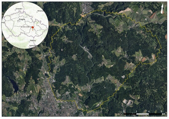
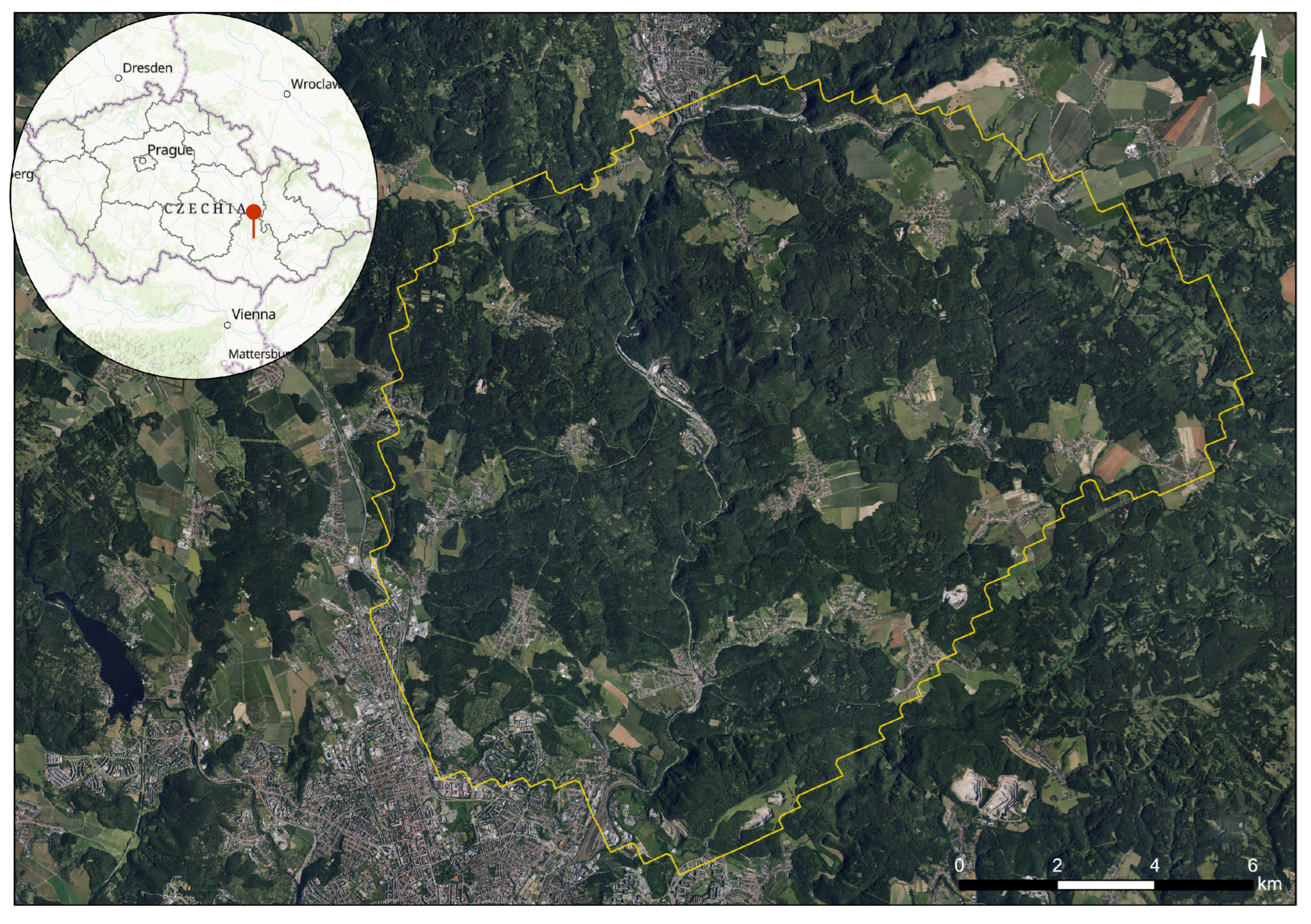
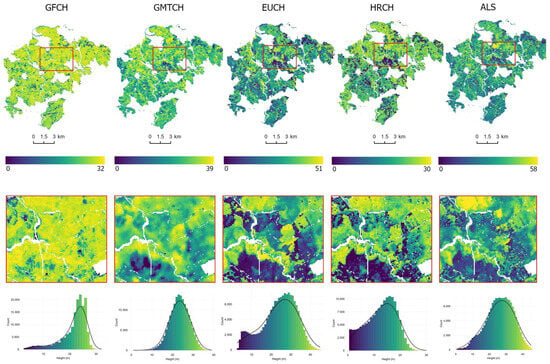
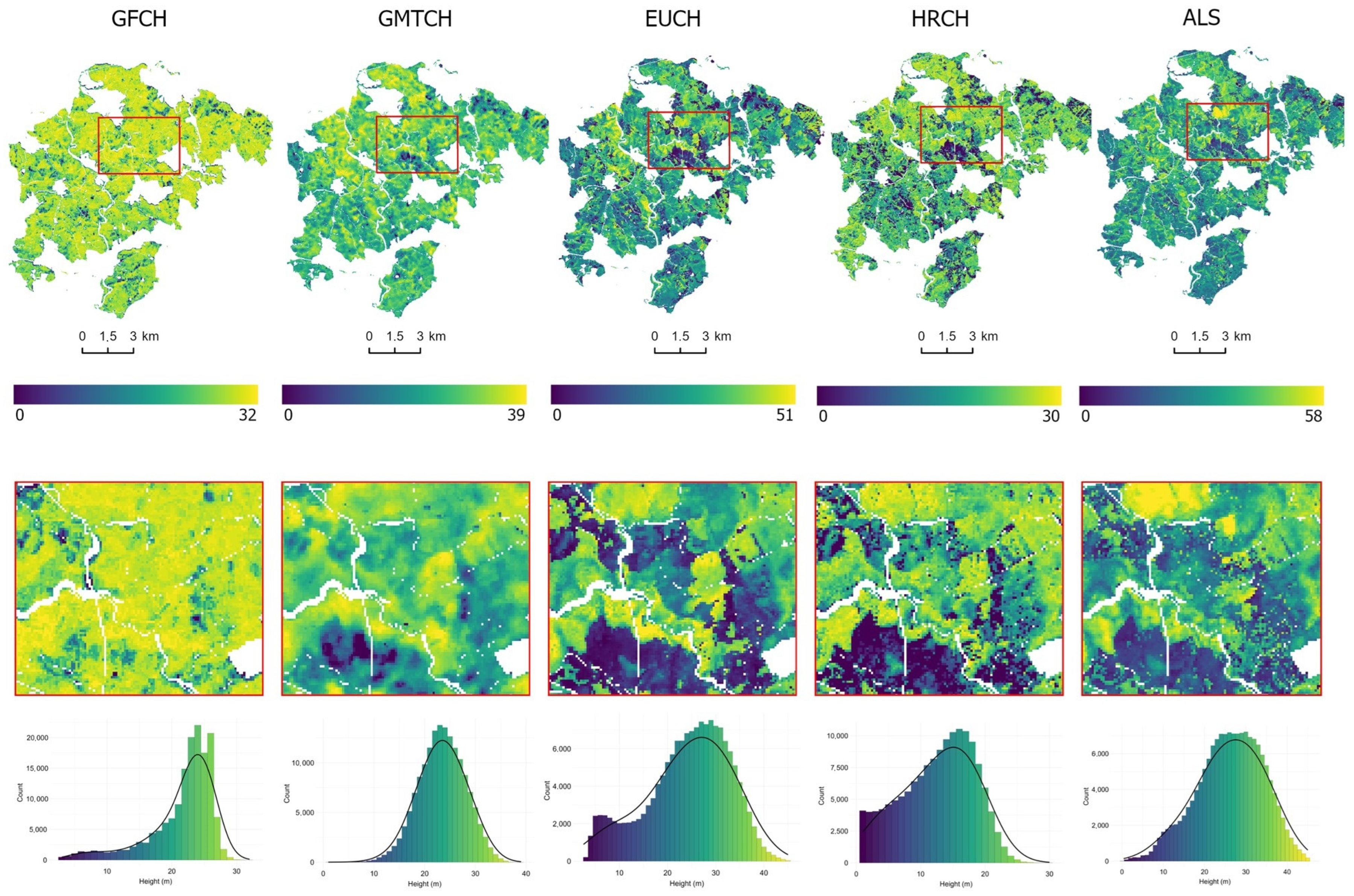
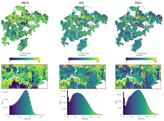
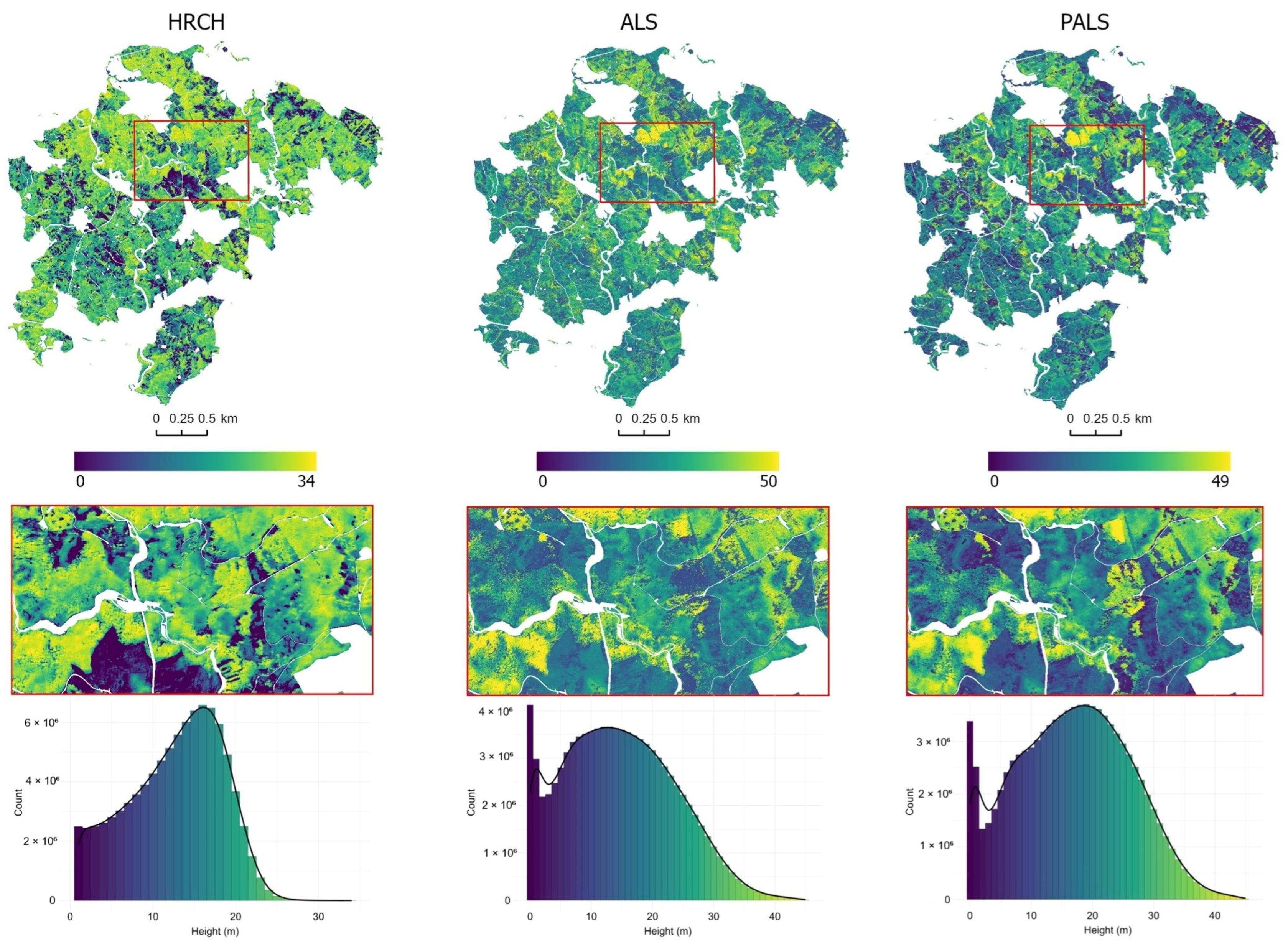
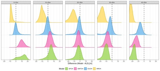
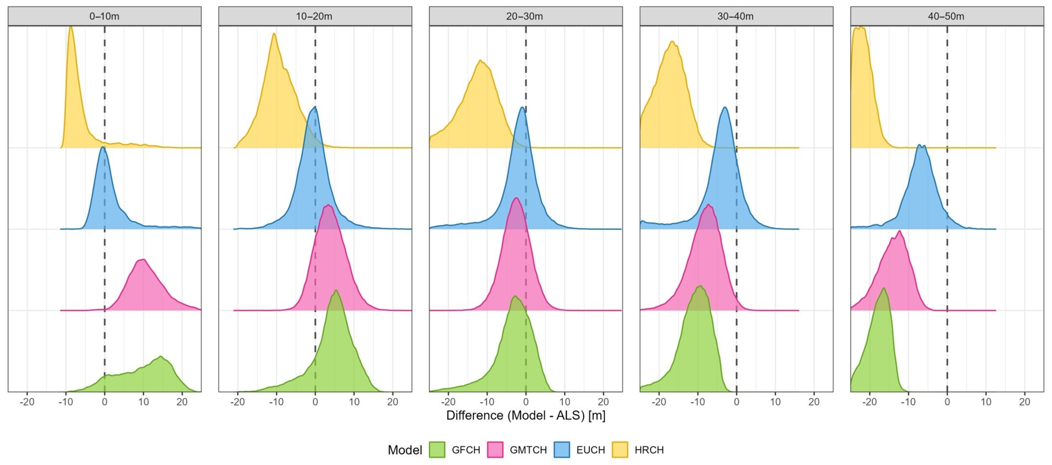
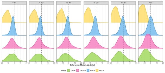
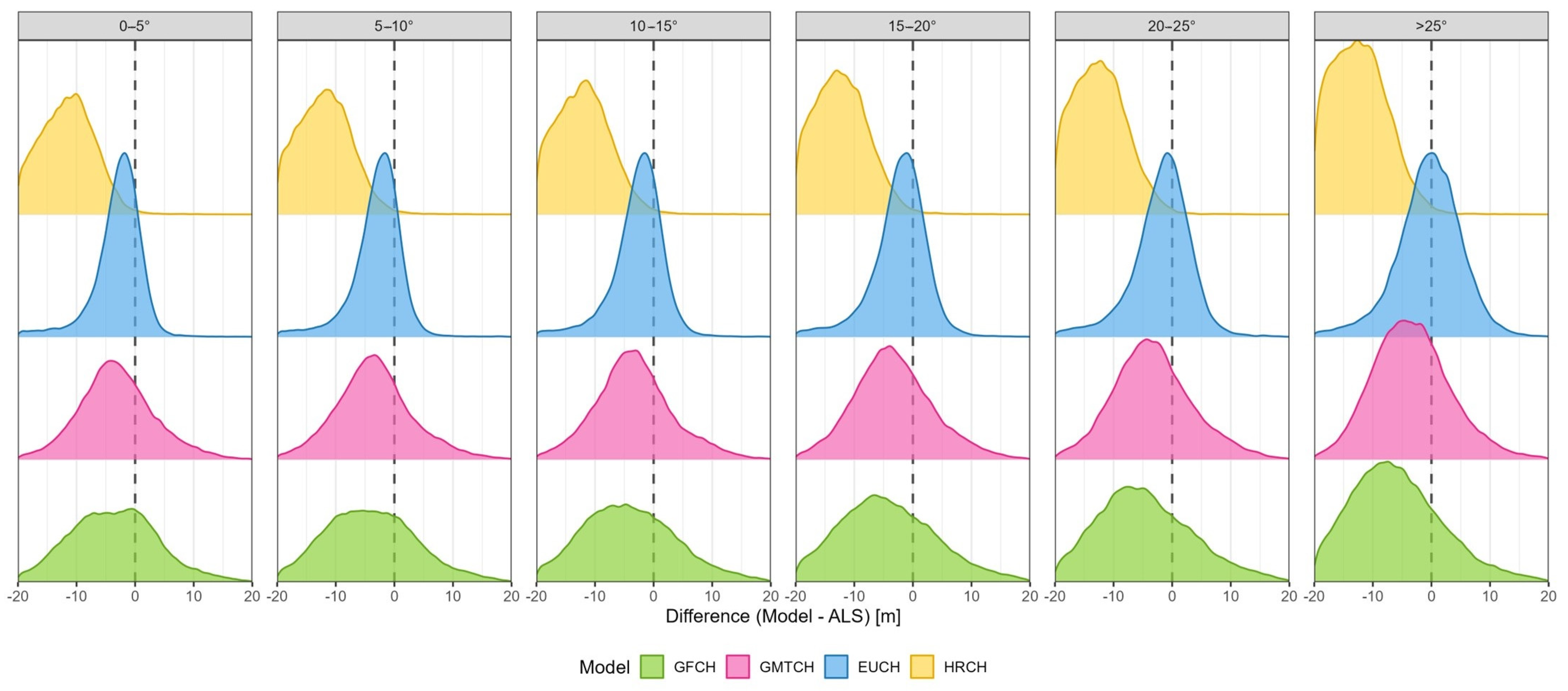
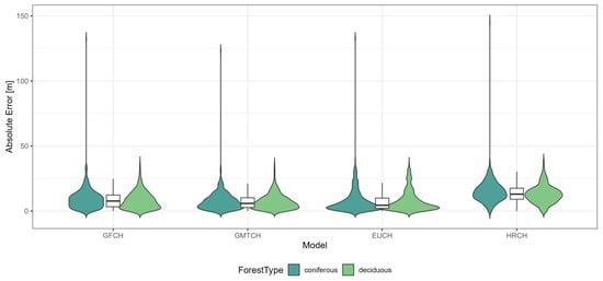
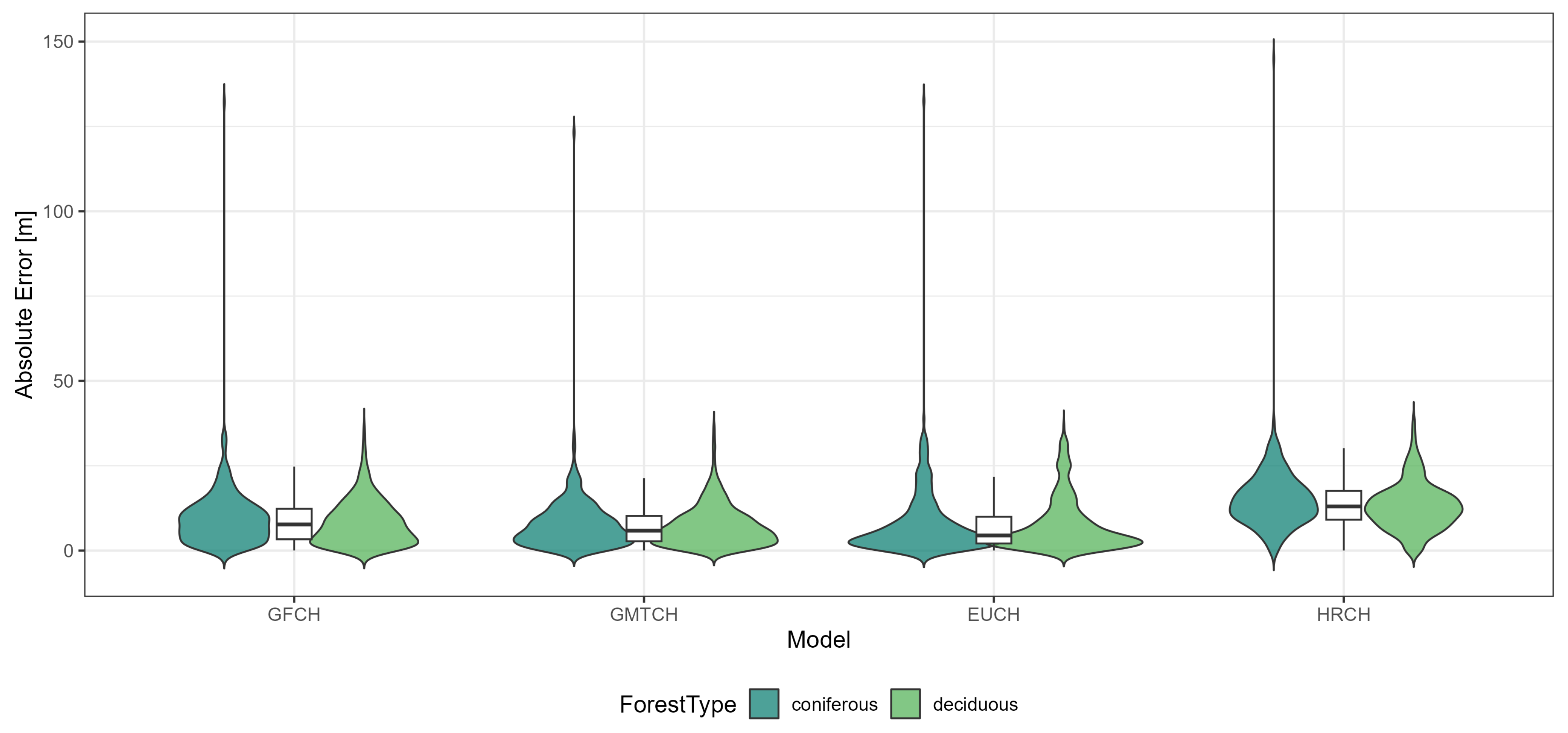
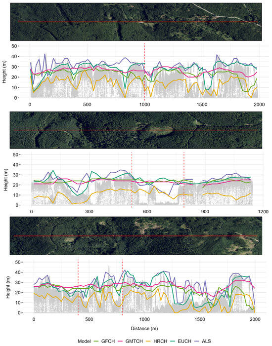
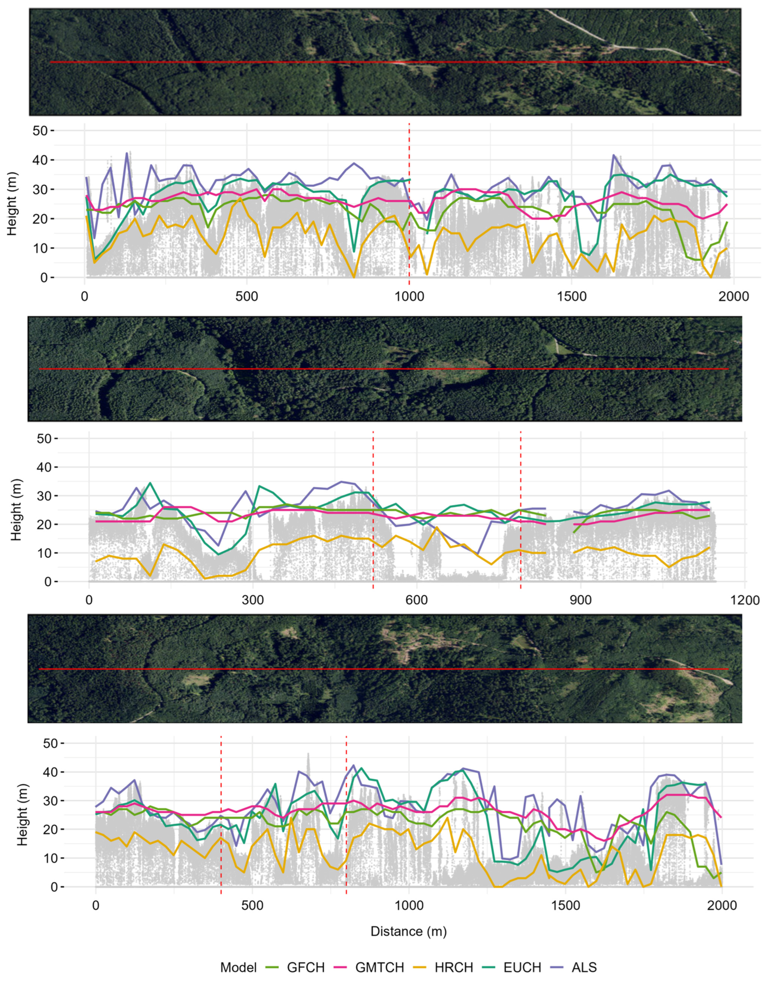
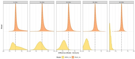
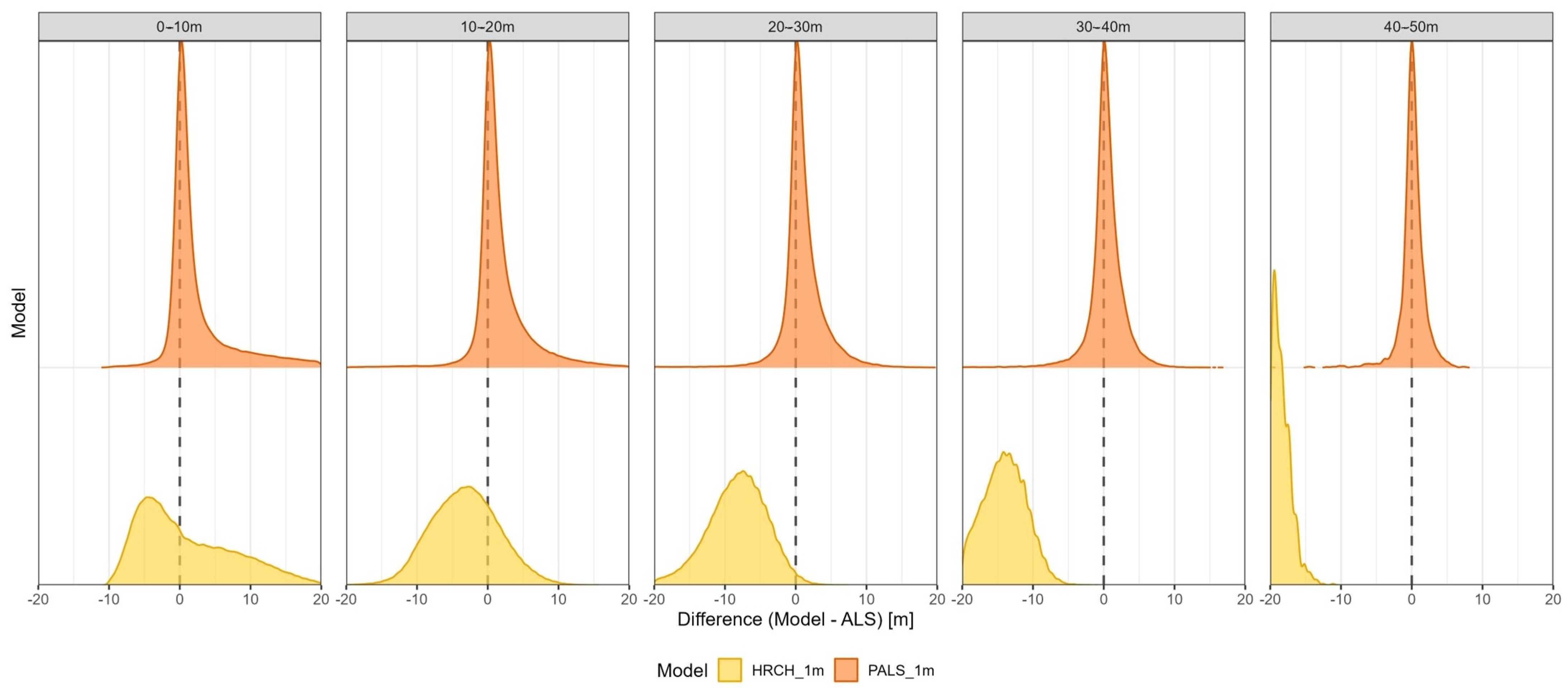
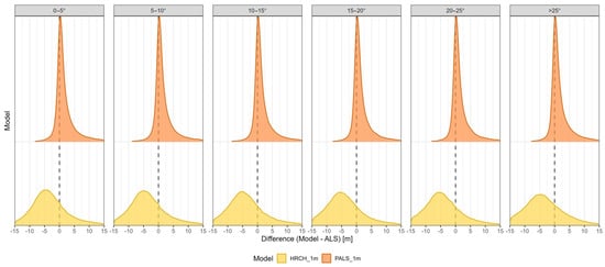
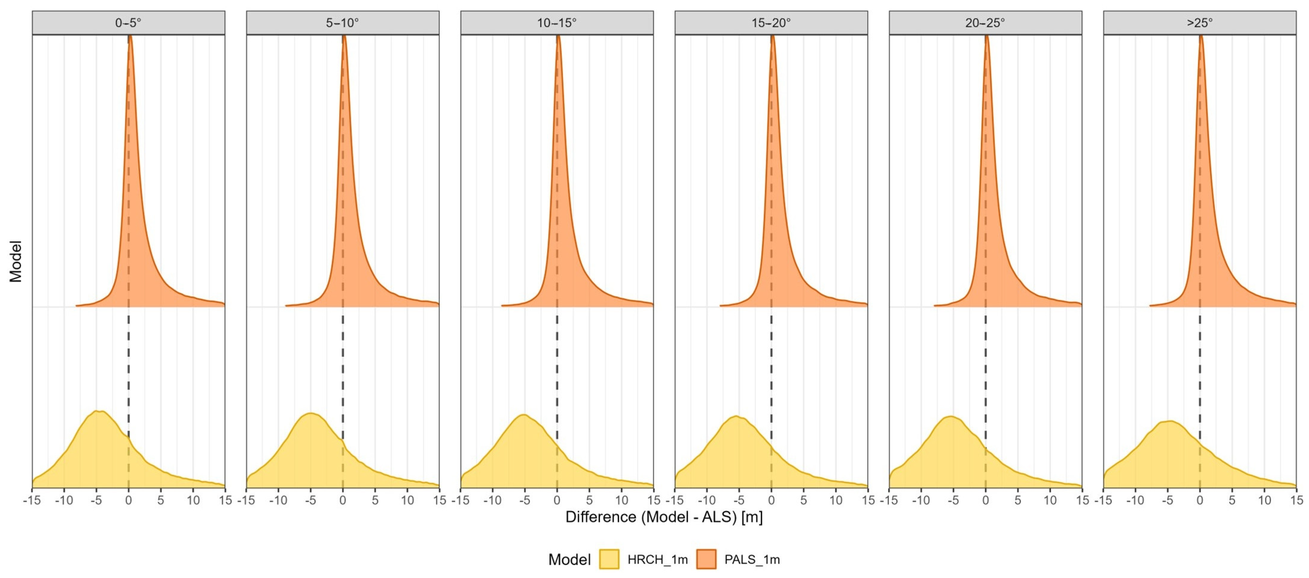
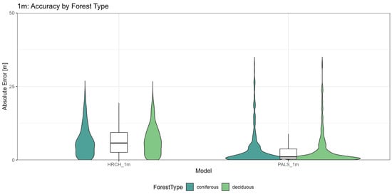
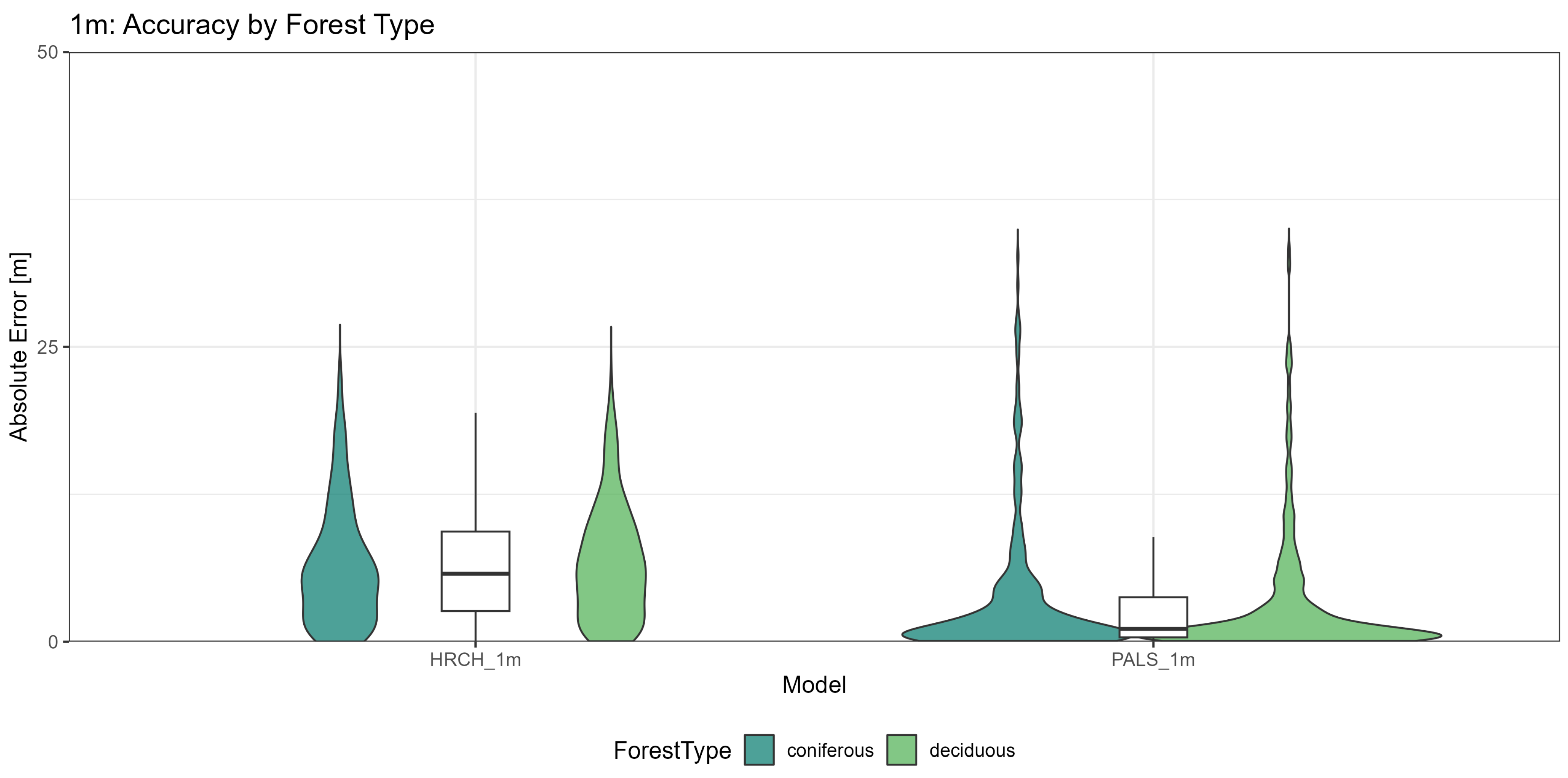
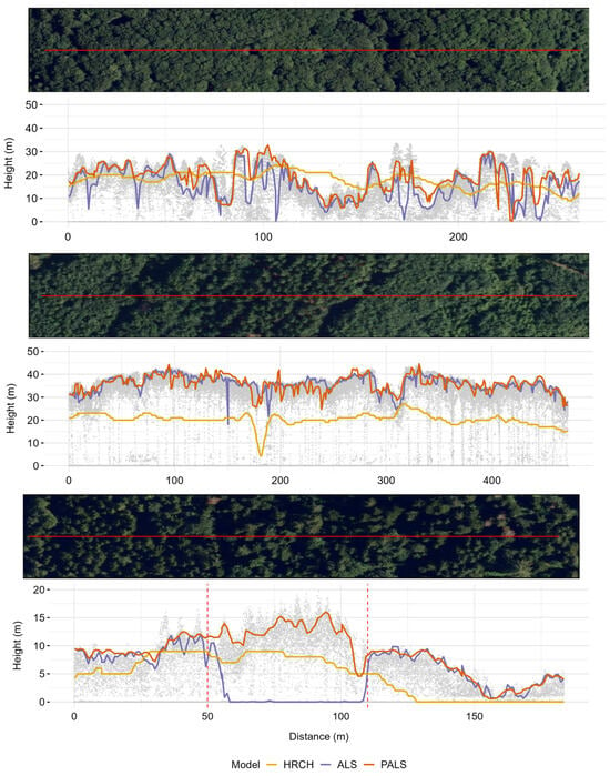
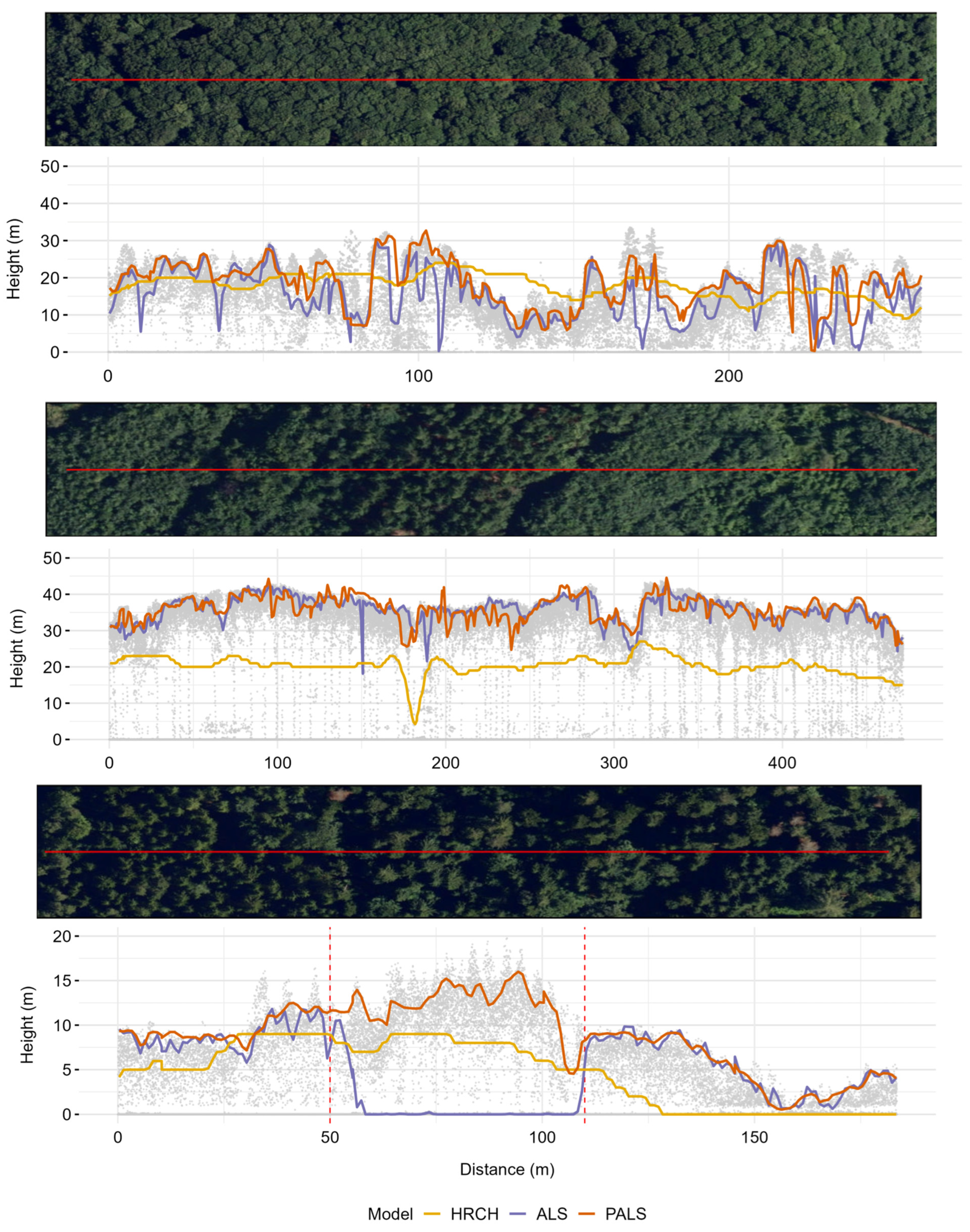
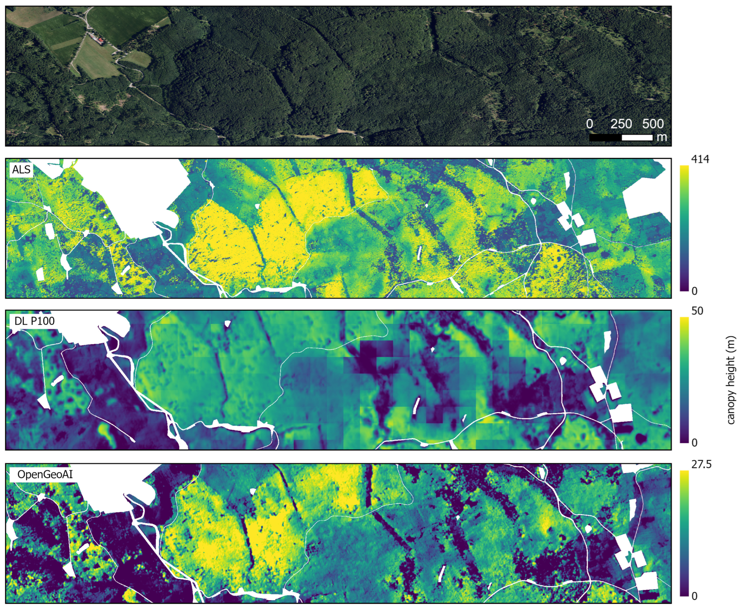
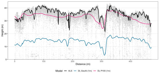
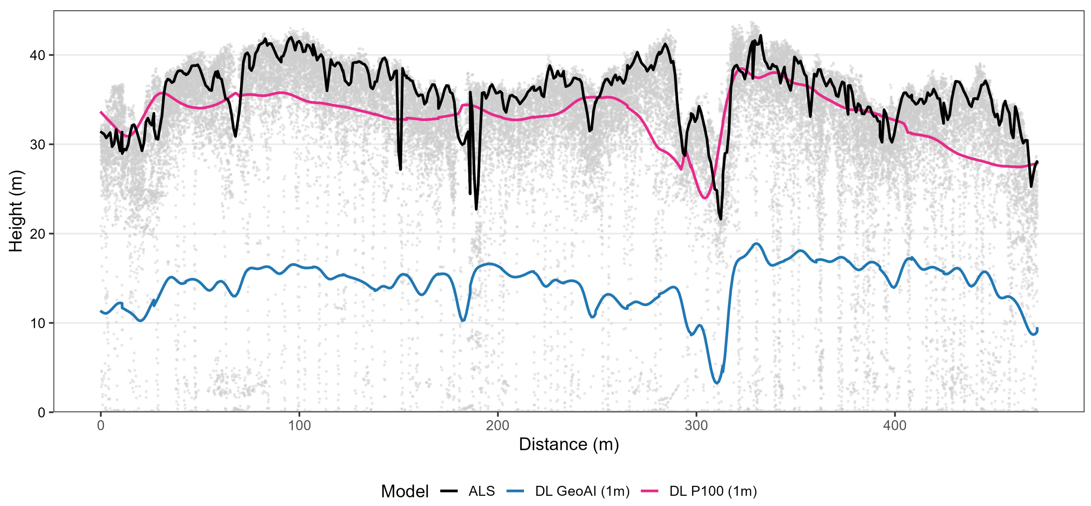
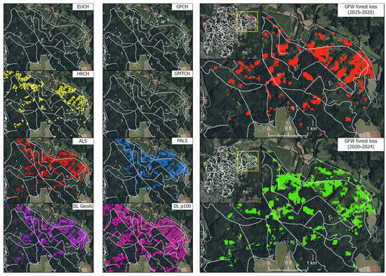
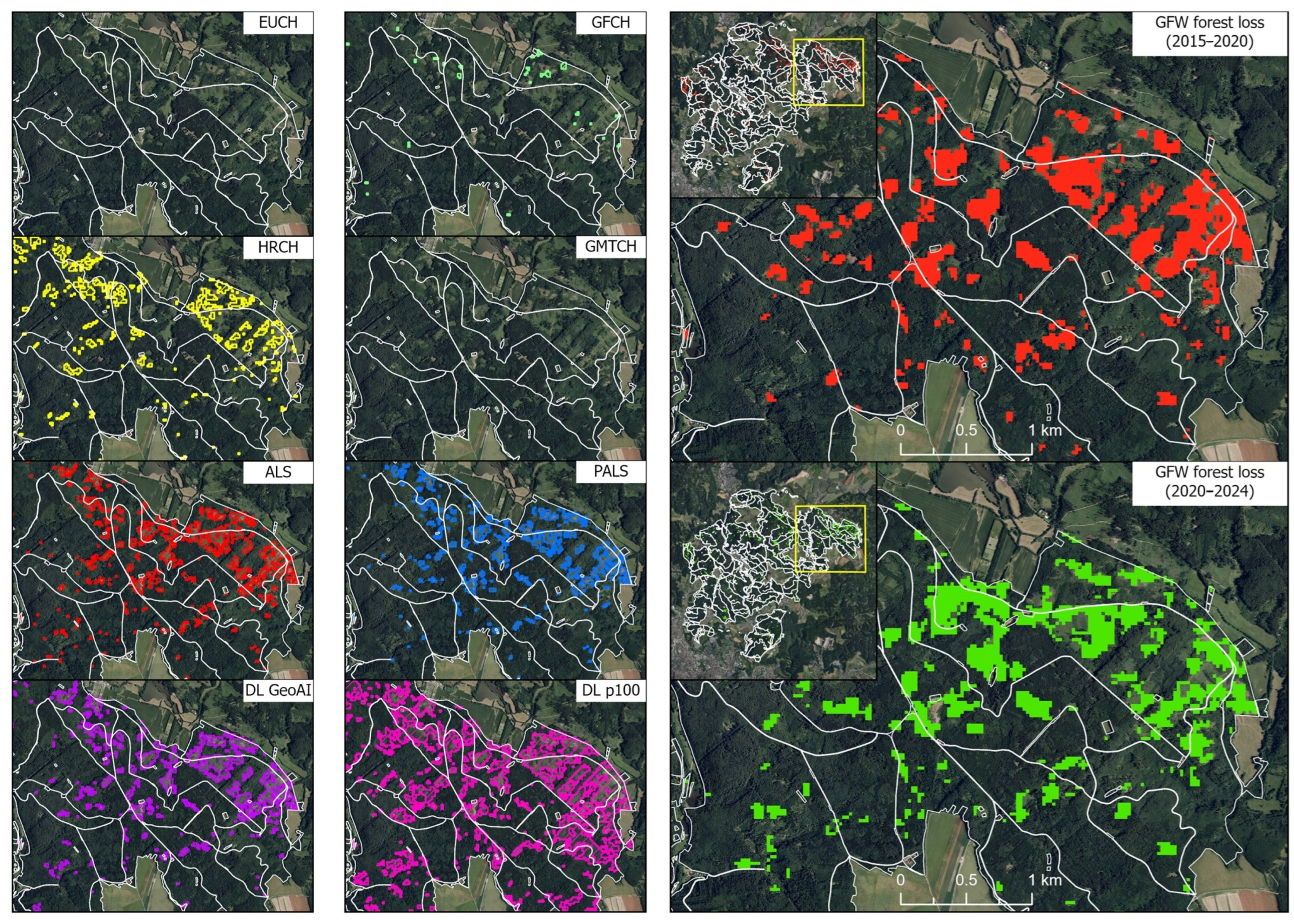
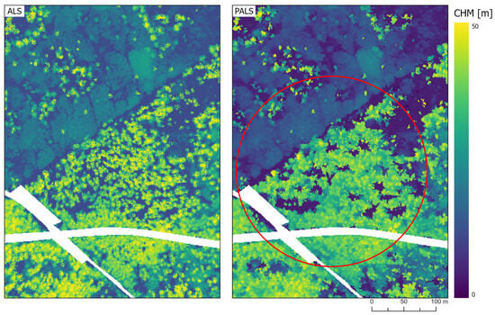
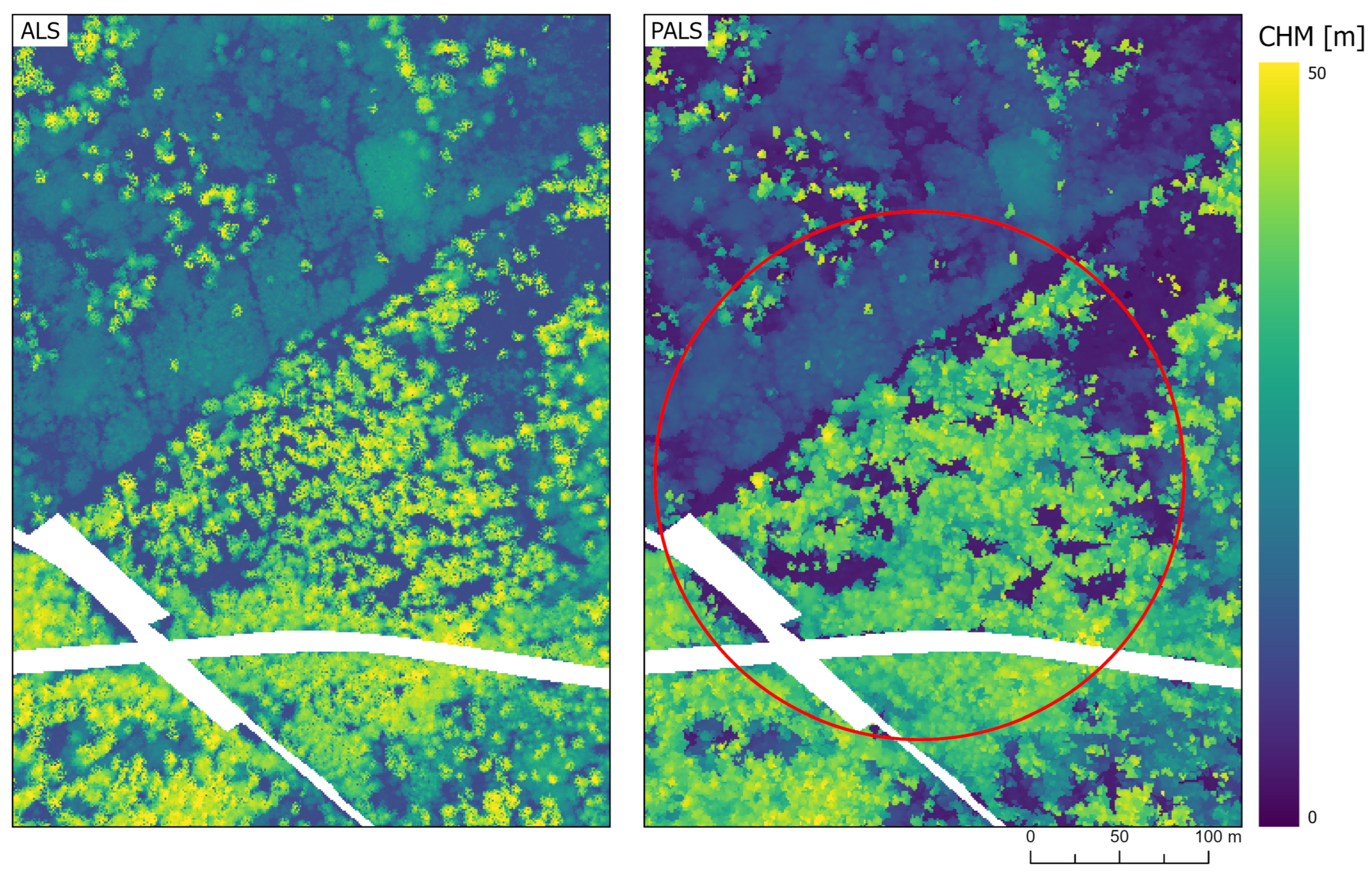

Disclaimer/Publisher’s Note: The statements, opinions and data contained in all publications are solely those of the individual author(s) and contributor(s) and not of MDPI and/or the editor(s). MDPI and/or the editor(s) disclaim responsibility for any injury to people or property resulting from any ideas, methods, instructions or products referred to in the content. |
© 2026 by the authors. Licensee MDPI, Basel, Switzerland. This article is an open access article distributed under the terms and conditions of the Creative Commons Attribution (CC BY) license.