


Highlights
What are the main findings?
- Ambient noise seismic interferometry successfully retrieves empirical Green’s functions containing the vertical component of Rayleigh waves and P-wave reflection energy, enabling passive seismic imaging of Antarctic drilling sites.
- The method provides stable and repeatable constraints on firn structure, ice thickness, and the ice–bedrock interface.
What are the implications of the main findings?
- Passive seismic imaging provides a fast and cost-effective tool for Antarctic drilling site selection and subsurface characterization.
- More generally, it can serve as a complement to active-source seismic methods, helping extend subsurface investigation to areas where conventional exploration is limited by logistical, environmental, or operational constraints.
Abstract
Antarctic drilling projects provide critical information for investigating ice-sheet stability, reconstructing paleoclimate evolution, and characterizing subglacial geological structures through ice-core and bedrock recovery. Drilling site selection currently relies on high-resolution geophysical methods such as radio echo sounding and active-source seismic methods; however, radar imaging near the ice–bedrock interface is limited by electromagnetic attenuation, while active-source seismic methods in polar regions are constrained by logistical complexity and high cost. To address these limitations, this study proposes a passive integrated imaging approach that integrates P-wave responses and vertical-component Rayleigh-wave information retrieved from continuous ambient noise recordings near drilling sites using seismic interferometry. Based on their distinct propagation characteristics, signal selection and processing workflows are developed to jointly image near-surface firn structure, ice-sheet thickness, and subglacial bedrock structure. Application to the Princess Elizabeth Land drilling project in East Antarctica demonstrates that high- signal-to-noise-ratio P-wave responses and vertical-component Rayleigh-wave signals can be retrieved from as little as 24 h of ambient noise data, while stacking the full 20-day record further suppresses incoherent noise and yields more reliable imaging of the ice–bedrock interface. These results indicate that passive seismic imaging provides a rapid, cost-effective, and environmentally friendly complement for drilling site selection and operational support.
1. Introduction
Antarctic drilling projects, through direct observations such as the recovery of ice cores and subglacial bedrock samples, provide critical constraints and observational evidence for studying the stability of the Antarctic ice sheet, reconstructing paleoclimate evolution, and revealing subglacial geological structures [1,2,3,4,5]. During drilling operations, key subsurface parameters, including the depths of the firn–ice transition zone and the ice–bedrock interface, as well as variations in ice density, provide essential constraints on drilling design and operational planning [2,4]. These parameters play a critical role in guiding decisions related to drill-string replacement strategies and drilling-fluid management strategies, thereby effectively reducing engineering risks such as drill-string failure and drilling-fluid loss [6,7,8,9]. Under the constraints of extremely low temperatures, limited logistical support, and short operational windows in Antarctica, obtaining rapid and reliable a prior information on the ice-sheet structure and subglacial bedrock geometry before or during drilling operations remains a key scientific and engineering challenge in Antarctic drilling research [10,11,12,13,14].
Geophysical methods such as radio echo sounding and active-source seismic methods are high-resolution techniques for investigating the structure of the Antarctic ice sheet and its underlying bedrock [13,15,16]. Radio echo sounding is characterized by high observational efficiency and relatively low operational cost, making it widely used for estimating the depth of the ice–bedrock interface [13,17]. However, RES imaging is sensitive to variations in firn and snow thickness, and strong electromagnetic attenuation at depth significantly limits its resolution at the ice–bedrock interface and within the underlying bedrock [16,18]. In contrast, active-source seismic methods offer greater investigation depth and higher imaging resolution [19,20,21,22,23]. Nevertheless, their application in Antarctic environments is strongly constrained by the need for active sources, high operational costs, and substantial logistical challenges [19,24,25].
Passive seismic methods use ambient seismic noise to characterize subsurface structure without requiring active seismic sources [26,27]. The theoretical foundation of passive seismic methods is seismic interferometry [28,29,30], which is based on the assumption of sufficiently diffuse or equipartitioned illumination of the receivers by ambient noise sources. Under this condition, the cross-correlation of continuous seismic recordings acquired at different receivers allows the retrieval of the inter-receiver Green’s function, thereby enabling imaging of the subsurface structure.
Based on the type of wavefield retrieved, passive seismic imaging can be classified into surface-wave imaging and body-wave imaging. Because ambient seismic noise is typically dominated by surface-wave energy, passive surface-wave imaging is generally more robust and reliable, and the dispersion characteristics of Rayleigh waves can be used to invert for subsurface shear-wave velocity structures [31,32,33]. Passive surface-wave imaging has been widely applied in many fields, including the imaging of crustal and lithosphere structures [34,35], near-surface engineering–geological investigations [31,36,37], monitoring of landslide and fault activity [38], and studies of glacier and ice-sheet structures [39,40,41].
In contrast, passive body-wave imaging remains more challenging, primarily due to the difficulty of satisfying the theoretical requirement of sufficiently uniform or isotropic illumination by ambient noise sources under practical field conditions. Moreover, body-wave energy contained in ambient seismic noise is generally weak, and body-wave responses can therefore only be retrieved within suitable frequency bands and under favorable observational conditions, enabling passive body-wave imaging [42,43,44,45]. Passive body-wave imaging has been applied to image sedimentary basins, fractures, and tectonic interfaces, and reservoir and crystalline bedrock structures [46,47]. Passive-source body-wave signals have been successfully used for subsurface investigations in polar environments, including applications of P-wave coda autocorrelation and receiver function methods to retrieve ice-sheet thickness, internal structure, basal low-velocity zones and seismic anisotropy [48,49,50,51].
The quality of passive seismic imaging is strongly controlled by the type, energy characteristics, and spatial distribution of ambient noise sources [27,34,52]. Compared with natural noise sources such as microseisms, which are regionally controlled and unevenly distributed in space and time, noise generated by engineering activities typically exhibits more localized source regions and similar propagation paths. These characteristics make engineering-related noise more favorable for wavefield identification and for enhancing the robustness and stability of seismic imaging [53]. During drilling operations, drilling-related ambient noise, generated by drill-bit interaction with the formation and vibrations of the drilling system, is characterized by broad frequency bandwidth, long duration, and relatively stable energy, and can therefore serve as a stable passive seismic source for imaging during drilling operations [54]. In oil and gas exploration and development, geothermal well evaluation, and mining engineering, passive seismic imaging based on drilling-induced noise provides an efficient and low-cost method for high-resolution characterization of detailed geological structures near wells [55,56,57].
Compared with conventional terrestrial applications, passive seismic imaging based on drilling-induced noise in Antarctic ice-sheet regions has particular value for the real-time detection of ice-sheet thickness and subglacial structures, thereby providing critical guidance for drilling operations, including decisions on drilling-tool replacement. However, due to differences in geological conditions and drilling systems, the frequency bandwidth, attenuation characteristics, and wavefield propagation of noise generated during ice-sheet drilling have not yet been systematically investigated. Furthermore, the spatial resolution and effective investigation range of this method for imaging ice-sheet and underlying bedrock structures remain to be quantitatively assessed and validated through field observations.
During the 2023–2024 Antarctic scientific expedition season, a joint Chinese–Russian drilling team conducted, for the first time, a drilling operation that penetrated the Antarctic ice sheet to the underlying bedrock in the core of a high-amplitude magnetic anomaly zone located at the northwestern margin of Princess Elizabeth Land, approximately 28 km south of Prydz Bay, East Antarctica. The drilling reached an ice thickness of 541.12 m and successfully recovered subglacial bedrock cores, together with direct measurements of basal ice temperature [2,4]. To assess the feasibility and achievable resolution of passive seismic imaging based on drilling-induced noise, a passive seismic survey line with a total length of approximately 2.1 km was deployed on both sides of the borehole during the drilling operations. The receiver line consisted of 100 vertical-component nodal seismometers, which continuously recorded ambient seismic noise for 20 days. The seismometers recorded not only natural microseisms, but also relatively stable engineering-related noise generated during drilling operations, such as drill-bit interaction with the ice sheet and vibrations of the drilling system associated with the drilling platform [2,6,7]. These different noise sources exhibit distinct spatial distributions and spectral characteristics, providing a basis for systematically comparing their propagation behavior and dispersion features within the ice sheet and evaluating their respective contributions to P-wave imaging and Rayleigh-wave imaging.
This study investigates passive seismic data acquired in polar ice-sheet drilling environments, which are characterized by the presence of multiple ambient noise sources. The drilling location and project background are first documented, followed by a detailed description of the drilling modes and power systems employed during operations, together with the associated types of drilling-related noise, including drill-bit–ice interaction noise and drilling system vibrations. The temporal–spectral characteristics, spatial distribution, and potential contributions of these noise sources to seismic imaging are then systematically analyzed. Based on the noise analysis results, we further developed a passive joint imaging method specifically designed for polar drilling environments, integrating P-wave responses and vertical-component Rayleigh-wave information. The proposed method integrates the robustness of vertical-component Rayleigh-wave imaging for resolving shallow structures with the higher energy and penetration depth of P-wave reflections for imaging deeper interfaces and is evaluated for its applicability to imaging the snow–firn–ice–bedrock system. This method does not require active sources and can be implemented concurrently with drilling operations, enabling environmentally responsible subsurface investigation while minimizing the impact of geophysical exploration on the Antarctic environment. The effectiveness and practical applicability of this method for investigating subglacial structures in Antarctica are further evaluated through comparisons between the joint imaging results and independent ice thickness measurements from drilling and radio echo soundings conducted near the borehole.
2. Study Area and Data Acquisition
During the 2023–2024 Antarctic scientific expedition season, a joint Chinese–Russian drilling team completed a borehole penetrating the ice sheet to the underlying bedrock at the northwestern margin of Princess Elizabeth Land, East Antarctica [2,4]. The drilling site (69.585591°S, 76.385165°E; elevation 680 m) is located approximately 28 km south of the Prydz Bay coast and lies within the central zone of a high-amplitude magnetic anomaly that extends across Princess Elizabeth Land and Mac Robertson Land (Figure 1a). The site is situated about 23.5 km from Zhongshan Station and approximately 24 km from Progress Station and its airfield (Figure 1b). The primary objective of the drilling was to recover subglacial bedrock in order to constrain the origin of the strong magnetic anomaly and characterize the basal properties. In addition, ice-core samples and borehole observations were used to validate and refine numerical models of the basal thermal regime in this region, thereby providing robust ground-truth data for subsequent studies of glacier dynamics and subglacial geology. Drilling operations were carried out between January and February 2024. On 24 February, the drill penetrated the ice sheet and reached the bedrock at a depth of 541.12 m, recovering a 0.48 m long bedrock core.
Figure 1.
Locations of the drilling site and the passive seismic survey line. (a) Location of the study area in the northwestern part of Princess Elizabeth Land, East Antarctic ice sheet, situated south of Zhongshan Station. The black line in (a) indicates the grounding line, and colors ranging from brown to dark blue represent bedrock elevation. (b) Location of the drilling site, approximately 28 km south of Zhongshan Station. (c) Two-dimensional linear passive survey line deployed around the drilling site, with an average receiver spacing of 20 m; the Chinese–Russian inland traverse route intersects the profile. (d) Drilling camp located near the center of the passive survey line, showing the drilling shelter, workshop, living shelters, and auxiliary facilities. (e) An ice-cutting drill bit at the lower part of the drilling rig.
The drilling operations employed an electromechanical, cable-suspended rotary drilling system, with drilling tools and techniques adapted in successive stages according to the stratigraphy of the ice column [2,4,7]. From the surface to a depth of 66.88 m, the snow–firn layer was penetrated by dry drilling using an auger core barrel (Figure 1e). Upon reaching impermeable glacier ice, coring was continued under fluid circulation using a kerosene-type drilling fluid (Jet A1). A polycrystalline diamond compact (PDC) bit was deployed for drilling debris-rich ice, whereas bedrock coring was ultimately performed with a toothed diamond bit. The drilling camp comprised a drilling shelter, workshop, living shelters, and auxiliary facilities, forming a mobile and self-contained inland drilling platform (Figure 1d). Following completion of drilling, a radio echo sounding survey was conducted near the borehole to constrain the local ice thickness and subglacial bedrock topography. The results indicate that the borehole is located near the crest of a subglacial bedrock hill, where the ice thickness is approximately 541 m at the drilling site, increases to ~575 m within a radius of ~200 m, and reaches up to ~670 m at distances of 1–2 km south of the borehole.
To evaluate the feasibility and imaging resolution of passive seismic methods for detecting the snow–ice and ice–bedrock interfaces, a passive survey line was deployed on both sides of the drilling site. The receiver line consisted of 100 vertical-component SmartSolo nodal seismometers with a natural frequency of 5 Hz, manufactured by SmartSolo Inc., Shenzhen, China. The average station spacing was 20 m; however, it was locally increased to 100 m on both sides of the borehole and to 80 m where the Chinese–Russian inland traverse route intersects the profile. The total length of the profile was approximately 2100 m (Figure 1c). This non-uniform deployment was mainly constrained by field conditions. In particular, larger station intervals were used around the drilling camp and along the vehicle route, where snow vehicles frequently passed, in order to reduce the risk of geophone damage. Compared with a conventional uniform array, such a non-uniform geometry may introduce additional uncertainty in the apparent velocity estimation of Rayleigh waves. To reduce this effect and to account for the stable-direction zones, the Rayleigh-wave dispersion curves were picked separately using several subarrays, and these subarrays were designed not to cross the drilling site or the strongly non-uniform sections. For P-wave reflection imaging, the non-uniform deployment may also reduce the fold coverage near the borehole compared with a uniform geometry, which could affect the local horizontal resolution of the retrieved reflection image.
The objective of deploying the passive seismic line was to develop a rapid, high-resolution, and cost-effective method that exploits drilling-induced noise and naturally occurring ambient seismic signals to image the geometry of the snow–ice and ice–bedrock interfaces beneath the borehole, and to assess its potential for providing guidance during drilling operations. A total of 20 days of ambient noise data were recorded during the drilling campaign, with a sampling interval of 4 ms, covering the period when the drilling depth advanced from 116 m to approximately 250 m. Drilling activities were ongoing during days 1–14 of the recording period, whereas drilling was suspended during days 15–20. The drilling camp comprised a drilling shelter, a workshop, living shelters, and auxiliary facilities; consequently, the ambient noise data include a variety of anthropogenic noise sources, such as vibrations generated by the subsurface ice-core drill bit and surface activities associated with the drilling shelter and auxiliary facilities.
3. Methods
3.1. Joint Imaging Framework
In this study, a joint passive imaging method integrating vertical-component Rayleigh-wave analysis and P-wave reflection imaging is applied to characterize the snow–ice interface and the ice–bedrock interface. This method fully exploits noise generated by anthropogenic activities associated with drilling operations, together with naturally occurring ambient microseismic background noise (Figure 2a). Based on passive seismic interferometry, virtual shot gathers are retrieved from ambient noise recordings, enabling the extraction of vertical-component Rayleigh-wave signals and P-wave reflection responses for imaging subsurface structural information without the need for controlled seismic sources. Rayleigh waves and P-wave reflections exhibit complementary characteristics in terms of propagation paths, investigation depth, and imaging resolution. Accordingly, joint inversion takes advantage of the high sensitivity of Rayleigh waves to shallow structures to achieve detailed imaging of the snow–ice interface, while exploiting the greater penetration depth of P-wave reflections to image the ice–bedrock interface and, potentially, structures within the underlying bedrock.
Figure 2.
Joint imaging method integrating passive Rayleigh waves and P-wave reflections. (a) Continuous recording of anthropogenic noise generated by drilling-related activities, together with naturally occurring ambient microseismic noise; (b) retrieval of Rayleigh-wave signals from ambient noise, followed by dispersion analysis, picking, and inversion to obtain the shear-wave velocity structure; (c) retrieval of P-wave reflection responses from ambient noise and subsequent P-wave reflection processing to produce stacked imaging sections; (d) construction of a subsurface geological model by integrating the shear-wave velocity structure obtained from vertical-component Rayleigh-wave inversion with the P-wave reflection imaging sections; (e) formulation of drilling strategies based on the constructed model, enabling the selection of appropriate drilling tools for the snow–firn layer, glacier ice, and bedrock, thereby improving drilling efficiency and reducing operational risk.
Rayleigh waves primarily propagate along the free surface and within shallow low-velocity layers, where their energy is concentrated and attenuates slowly, making them highly sensitive to variations in the elastic properties of near-surface media. In addition, Rayleigh waves exhibit pronounced dispersive behavior, with different frequency components corresponding to different effective penetration depths. Frequency–phase velocity relationships are estimated using methods such as the phase-shift technique [31], dispersion curves are identified and picked, and dispersion inversion is then performed to convert the observed dispersive characteristics into a continuous depth-dependent shear-wave velocity model, thereby constraining the physical properties of shallow layers and the depths of key interfaces (Figure 2b). The Rayleigh-wave imaging results effectively delineate the shear-wave velocity structure of the snow layer, firn layer, and shallow glacier ice. Through empirical velocity–density relationships, the corresponding density variations with depth can also be derived, providing a reference for determining the appropriate transition from snow drilling to ice drilling during operations. In addition, the shallow structural and velocity information obtained from Rayleigh-wave imaging serves as an important constraint for subsequent P-wave reflection imaging.
Passive P-wave reflection imaging primarily exploits P-wave reflection energy retrieved from ambient noise recordings. Based on passive seismic interferometry for P-wave reflections, P-wave reflection responses are retrieved from the noise data and subsequently processed through denoising, velocity analysis, migration, and stacking to produce imaging sections (Figure 2c). Because P-wave reflections propagate three-dimensionally within the subsurface and are more sensitive to impedance contrasts, they provide enhanced capability for detecting subsurface interfaces, particularly at greater depths. This makes P-wave reflection imaging well suited for delineating the geometry and relief of deep interfaces and for resolving internal structural features. In the present application, P-wave reflection imaging enables clear characterization of the ice–bedrock interface, including its geometric morphology and undulations, and reveals the principal structural features within the underlying bedrock. Compared with Rayleigh waves, P-wave reflections offer distinct advantages in terms of investigation depth and imaging resolution of deep interfaces, and thus constitute a key tool for deep structural imaging.
A comprehensive subglacial geological model encompassing the snow layer, firn layer, glacier ice, and bedrock is constructed by integrating the shear-wave velocity structure obtained from vertical-component Rayleigh-wave inversion with the migrated P-wave reflection imaging results (Figure 2d). This model has direct practical value for drilling operations. The shallow shear-wave velocity structure is used to assess the mechanical properties of different media and the associated drilling difficulty, to constrain the position of the snow–ice interface, and to guide the selection of appropriate drilling tools. In contrast, the P-wave reflection imaging results provide critical constraints on the depth of the ice–bedrock interface, the structural characteristics of the bedrock, and the identification of potential engineering risks. Based on the subsurface model established through joint imaging, a stratified and differentiated drilling plan can be formulated before drilling. This plan allows the adoption of tailored drilling strategies and tool configurations for the snow–firn layer, glacier ice, and bedrock, respectively (Figure 2e), thereby effectively improving drilling efficiency and reducing the probability of tool failure and overall engineering risk.
3.2. Passive Surface-Wave Interferometry and Stable-Phase Theory
Passive surface-wave interferometry retrieves the Green’s function between two receivers by cross-correlating their recorded wavefields. To illustrate the basic principle, for a one-dimensional lossless medium with two receivers at and and an impulsive source at , the cross-correlation of the two recorded Green’s functions suppresses the propagation path common to both records and retrieves the inter-receiver response [29]:
where denotes the Green’s function observed at as if an impulsive source were located at , and denotes convolution. Because the second term is time-reversed, the operation is equivalent to cross-correlation. This relation shows that the absolute source time and the source–receiver propagation path do not need to be known explicitly; they are removed during the correlation process. When the source emits a non-impulsive wavelet rather than an impulse, the recorded fields become
and
The cross-correlation of the two recorded fields then yields the Green’s function convolved with the autocorrelation of the source wavelet:
where is the autocorrelation of the source wavelet. This formulation also holds when the source signal is a noise sequence rather than a deterministic transient wavelet. In ambient noise interferometry, the observed wavefield is generally produced by multiple simultaneously acting noise sources. For a set of mutually uncorrelated noise sources , the recorded noise field at either receiver can be written as
If the noise sources are mutually uncorrelated, their correlation satisfies
where is the Kronecker delta, is the autocorrelation of the noise source function, and denotes ensemble averaging, which is commonly approximated by sufficiently long-time averaging in practice. Under this assumption, the nonphysical cross-terms vanish, and the cross-correlation of the two observed ambient noise records becomes
Equation (7) indicates that the cross-correlation of two passive noise records retrieves a time-symmetric response, consisting of the causal Green’s function and its time-reversed counterpart, convolved with the autocorrelation of the noise source. The causal or acausal part can be extracted depending on the dominant illumination direction.
For two- and three-dimensional media, the retrieval of the inter-receiver response does not require equal contributions from all source azimuths. Instead, the dominant contributions arise from stationary-phase regions. Following the stationary-phase interpretation, for a scatterer or secondary source at distance from receiver , the wavefield can be expressed as
where is the propagation velocity. The cross-correlation of and is dominated by sources located in the Fresnel zone around stationary points, where the traveltime difference is stationary with respect to the source coordinate . Sources outside these zones interfere destructively and contribute negligibly to the retrieved Green’s function. For surface-wave interferometry, this implies that, even with a non-uniform source distribution, the fundamental-mode Green’s function can be reliably retrieved as long as the stationary-phase regions are adequately illuminated.
In practice, to mitigate amplitude and spectral imprint effects from the ambient noise sources, we employ cross-coherence rather than direct cross-correlation. The cross-coherence is computed in the frequency domain as
where is angular frequency and the superscript denotes complex conjugation. This spectral normalization suppresses the influence of dominant noise sources and produces more uniform-amplitude virtual shot gathers, which facilitates subsequent dispersion analysis.
3.3. Passive Reflection Seismic Interferometry
The fundamental principle of passive-source reflected-wave interferometry is that the reflection response between receivers can be retrieved by autocorrelating or cross-correlating the transmission wavefields generated by subsurface sources and recorded at the receivers, thereby eliminating the propagation effects along paths common to the wavefields. Considering that a one-dimensional model consisting of a free surface, a single homogeneous lossless layer, and an underlying homogeneous lossless half-space, a unit impulsive source located in the lower half-space generates an upward-propagating plane wave, which propagates through the medium and reaches the free surface.
For a lossless layered medium, the relationship between the global reflection response and the global transmission response can first be expressed in the frequency domain as [29]
where and denote the Fourier transforms of the global reflection response and the global transmission response , respectively, and the superscript denotes complex conjugation. Transforming Equation (10) back to the time domain gives the one-dimensional reflected-wave interferometric relation
where is the Dirac delta function and denotes temporal convolution. Equation (11) indicates that the causal reflection response , together with its time-reversed counterpart , can be retrieved from the autocorrelation of the global transmission response.
When the impulsive source is replaced by a passive noise source, the recorded wavefield can be written as , where is the source time function. Under ensemble averaging, Equation (11) becomes
where is the autocorrelation of the noise source time function, and denotes ensemble averaging, which is commonly approximated by long-time averaging in practical passive seismic applications.
In two- and three-dimensional settings, wave propagation is no longer confined to a single ray path; however, the reflection response can still be retrieved through the elimination of common propagation paths. Under the assumption that the noise sources are sufficiently distributed in space and mutually uncorrelated in time, two-dimensional reflected-wave seismic interferometry can be written as
where denotes the reflection response recorded at receiver due to an impulsive source located at , is the autocorrelation of the source time function. and denote the horizontal components of and , respectively. and are the recordings at receivers located at and , respectively. This result demonstrates that reflected-wave seismic interferometry enables the retrieval of primary reflections from ambient noise, thereby providing a theoretical basis for subsequent noise-based reflection imaging.
4. Ambient Noise Characteristic Analysis
This study systematically analyzes the time–frequency characteristics and spatial distribution of different types of recorded ambient noise. The continuous 20-day noise record from receiver 51 located near the drilling site (Figure 3a) contains multiple events with markedly elevated energy. In contrast, the continuous 20-day noise record from the first receiver located far from the drilling site is shown in Figure 3b; although the overall energy level is significantly lower than that recorded near the drilling site, multiple high-energy events are still observed.
Figure 3.
(a) Twenty-day ambient noise record from receiver 51 located near the drilling site; (b) twenty-day ambient noise record from receiver 1 located far from the drilling site; (c) PSD of the noise record at receiver 51; (d) PSD of the noise record at receiver 1.
To quantitatively characterize the frequency bandwidth of the noise sources and their temporal variability, power spectral density (PSD) analysis was performed on the raw ambient noise records, providing a basis for subsequent retrieval of vertical-component Rayleigh-wave signals and P-wave reflection response, as well as for the rational selection of denoising parameters. Noise records from receiver 51, located approximately 50 m from the drilling site, and receiver 1, located about 1090 m away, were selected for PSD estimation, with the results shown in Figure 3c,d, respectively. The PSD results indicate that harmonic signals generated by mechanical vibrations persist near the drilling site throughout the 20-day observation period. These signals show persistent harmonic peaks with an approximately regular spacing of 12.5 Hz. Although the component near 12.5 Hz is relatively weak, higher harmonics, especially near 25, 37.5, and 75 Hz, are more prominent. Therefore, the fundamental frequency is inferred to be approximately 12.5 Hz from the harmonic spacing rather than from the strongest spectral peak. The corresponding energy is markedly weaker at the receiver located farther from the drilling site, indicating that the signals originate from the drilling area and associated human activities. Because these harmonic signals persist even after drilling ceased after day 15, they are unlikely to have been generated directly by the drill bit. They are more plausibly attributed to continuous mechanical vibrations from nearby equipment, such as the power-generation module or other auxiliary facilities near the borehole.
To further investigate the detailed multi-trace characteristics of the stationary noise and high-energy events, local enlarged displays of representative stationary-noise and high-energy-event segments selected from Figure 3a are presented. One representative high-energy event was selected, and a 20 s segment of its waveform is displayed in Figure 4b, together with a 1 s record section from the same time window (Figure 4d). Based on the combined characteristics of the single-trace records and the record sections, this event exhibits features consistent with excitation by an approximately impulsive source near the drilling site, including clear Rayleigh-wave arrivals, indicating that it was produced by strong vibrations associated with engineering activities near the borehole. A relatively stationary time interval from the noise record at receiver 51 is shown in Figure 4a, and the corresponding 1 s record section is presented in Figure 4c. During this interval, the noise energy distribution is stable and lacks impulsive events. In conjunction with the power spectral density results shown in Figure 3c, which demonstrate the persistent presence of mechanically induced signals around the drilling site throughout the 20-day observation period, it can be inferred that this type of stationary noise is primarily generated by continuous mechanical vibrations, such as those associated with the power-generation module at the drilling camp. After drilling operations ended on Day 15, the amplitudes recorded by the near-field geophones remained comparable to those observed during active drilling and were substantially higher than those recorded by the far-field geophones. Inspection of the raw waveforms further shows that strong Rayleigh-wave energy persisted at the drilling camp after drilling stopped. Considering that the camp generator continued to operate after the cessation of drilling, we infer that these signals were most likely continuous Rayleigh waves generated by the power-generation module.
Figure 4.
(a) Enlarged single-trace waveform of a 20 s stationary-noise segment selected; (b) enlarged single-trace waveform of a 20 s noise segment containing high-energy events; (c) multi-trace record section of a 1 s stationary-noise segment, showing that the energy is strongest near the drilling site in the middle of the survey line and varies only slightly with time; (d) multi-trace record section of a 1 s high-energy event segment, indicating that drilling-related noise is still present during the high-energy event, while the high-energy event itself appears as a record generated by an approximately impulsive source.
To investigate the influence of drilling and other anthropogenic activities on the recorded ambient noise, the receivers were grouped into five categories according to their distance from the drilling site, from farthest to nearest. The first and second groups comprise receivers 1–10 and 91–100, respectively, with an average distance of approximately 950 m from the borehole; their corresponding spectral distributions are shown by the red curves in Figure 5a,b. The third and fourth groups include receivers 26–35 and 66–75, with an average distance of about 450 m, and their spectra are represented by the green curves in Figure 5a,b. The fifth group consists of receivers 46–55, located within ~150 m of the drilling site, and their spectra are indicated by the blue curves in Figure 5a,b. Comparison of the spectral energy at different distances from the drilling site shows that energy in the 10–110 Hz band increases markedly as the receivers approach the borehole, indicating that drilling activities generate substantial energy in this frequency range. In contrast, the energy in the 0–10 Hz band exhibits little dependence on the distance between the receivers and the drilling site, suggesting that this low-frequency energy is largely unrelated to local anthropogenic activity and is more likely associated with natural microseismic sources.
Figure 5.
(a) Power spectral density of the 20-day noise records from receivers 1–10, 26–35, and 46–55; (b) power spectral density of the 20-day noise records from receivers 46–55, 76–85, and 91–100.
5. Ambient Noise Imaging near a Drilling Site
5.1. Rayleigh-Wave Response Retrieval and Shear-Wave Velocity Inversion
Based on the noise analysis, persistent anthropogenic noise is observed near the drilling site, as illustrated in Figure 6a. During observation intervals not affected by pronounced high-energy events, the noise records are dominated by coherent linear Rayleigh-wave signals originating from the drilling area. These waves propagate with an apparent velocity of approximately 1400 m/s, which is consistent with typical Rayleigh-wave velocities in snow–ice environments. Beamforming analysis was performed on the full-day noise records, with the results shown in Figure 6b. The scanning frequency range was set to 24–25 Hz, as the drilling-related noise energy was clearly identifiable within this frequency band. The scanning velocity was selected by jointly considering the phase velocities obtained from the preliminary dispersion analysis and the degree of energy focusing in the beamforming results, resulting in an optimal value of 1400 m/s. To reduce the influence of near-field sources, a receiver array located approximately 200 m from the drilling site was selected. The beamforming results for the receiver array indicated by the blue dashed box show that the dominant energy arrives from the 0° direction, whereas the results for the array indicated by the green dashed box show dominant energy from the 180° direction. Considering that both receiver arrays indicate energy arriving from the direction of the drilling site, it can be concluded that drilling operations and associated anthropogenic activities are interpreted as the primary source of energy in this frequency band.
Figure 6.
(a) A representative 2 s segment of ambient noise data from the first day of recording; (b) beamforming results for the first-day noise record, with the receiver aperture used for beamforming indicated by the blue and green dashed boxes above; the analysis was performed over a frequency band of 24–25 Hz with an assumed velocity of 1400 m/s, and the results indicate that the dominant noise energy is concentrated near the drilling site; (c) the 51st virtual shot gather retrieved from the first-day noise record using cross-coherence seismic interferometry, with a 60 s time window and the first 1 s displayed; (d) virtual shot gather after 0–80 Hz band-pass filtering, resulting in effective suppression of high-frequency noise and an enhanced signal-to-noise ratio of Rayleigh waves; (e) dispersion curve derived from Rayleigh-wave signals within the red-boxed area, outlined by the red lines in panel (d), using the phase-shift method, with the white scatter points indicating the actually picked dispersion points.
For the receiver arrays comprising receivers 1–50 and 51–100, most of the Rayleigh-wave energy arriving from the drilling direction lies within the phase-stable region of the cross-correlation functions. Therefore, the full-day ambient noise records are suitable for passive seismic interferometry to retrieve Rayleigh-wave signals. After applying standard preprocessing steps to the noise data, including demeaning, detrending, and suppression of strong-amplitude signals in the time–frequency domain, Rayleigh-wave virtual shot gathers were retrieved using cross-coherence-based seismic interferometry, as shown in Figure 6c. The virtual source was positioned at receiver 51, and a correlation time window of 60 s was used. After applying a 0–80 Hz band-pass filter to the virtual shot gathers (Figure 6d), Rayleigh-wave signals within the red-boxed area were selected for dispersion-spectrum calculation using the phase-shift method [31], resulting in the dispersion image shown in Figure 6e. The fundamental-mode dispersion curve exhibits a high signal-to-noise ratio and can be reliably identified over a frequency range of 3–55 Hz, with corresponding phase velocities ranging from approximately 1200 to 1700 m/s. Therefore, in the subsequent inversion, only the picked fundamental-mode Rayleigh-wave dispersion curves were used to constrain the shear-wave velocity structure. These high-frequency, high-signal-to-noise-ratio dispersion curves provide a robust basis for subsequent high-resolution shear-wave velocity inversion.
To investigate the influence of drilling and related engineering activities on Rayleigh-wave imaging, dispersion curves were obtained from virtual shot gathers at different distances from the drilling site, as shown in Figure 7. The results reveal pronounced distance-dependent differences in both the frequency distribution and energy characteristics of the dispersion curves. At a distance of approximately 50 m from the drilling site (Figure 7a,d), the dispersion curves exhibit clear and continuous energy distributions in both the low-frequency band (5–25 Hz) and the mid- to high-frequency band (25–55 Hz), with relatively high signal-to-noise ratios. As the distance increases to about 150 m (Figure 7b,e), energy in the low-frequency band remains stably identifiable, whereas high-frequency energy in the 25–55 Hz band is significantly attenuated, and the dispersion curves in this frequency range become increasingly scattered and discontinuous. At a distance of approximately 250 m from the drilling site (Figure 7c,f), the dispersion energy is largely confined to the low-frequency range of 5–25 Hz, while high-frequency energy cannot be clearly observed, making it difficult to extract reliable high-frequency dispersion information.
Figure 7.
Dispersion curves at different distances from the drilling site. Panels (a,d) show the dispersion curves at approximately 50 m from the drilling site; panels (b,e) correspond to distances of approximately 150 m; and panels (c,f) represent dispersion curves at approximately 250 m from the drilling site. The colored horizontal segments indicate the receiver ranges selected for calculating the corresponding dispersion curves.
The spatial variation in dispersion characteristics indicates that drilling operations and associated mechanical vibrations strongly influence the frequency bandwidth of the vertical-component Rayleigh-wave energy. Low-frequency Rayleigh-wave energy (5–25 Hz) is identifiable at all distances, suggesting that this band is primarily governed by ambient background vibrations or regional noise sources and is characterized by relatively stable propagation and low attenuation. In contrast, high-frequency Rayleigh-wave energy in the 25–55 Hz band is well developed only in the immediate vicinity of the drilling site and decays rapidly with distance, becoming difficult to identify at distances of approximately 150 m. This observation indicates that the high-frequency band is predominantly excited directly by drilling and engineering activities and is strongly affected by high-frequency attenuation. Consequently, drilling operations and related mechanical vibrations are inferred to act as an effective source of high-frequency Rayleigh-wave energy within a radius of approximately 150 m from the drilling site, beyond which the contribution of high-frequency components to dispersion analysis diminishes rapidly.
The shear-wave velocity structure was inverted using a genetic algorithm (GA), which belongs to a class of nonlinear global optimization techniques. Compared with conventional linear inversion approaches, GA-based methods are capable of exploring the global solution space within prescribed parameter bounds, are less susceptible to local minima, and show reduced dependence on a priori information from the initial model [58,59]. The number of iterations is a key parameter controlling inversion convergence and computational efficiency. A sufficiently large number of iterations helps mitigate premature convergence to local minima. The maximum number of iterations was set to 20,000 to allow a sufficiently broad search by the genetic algorithm. This value was used only as an upper bound. In practice, the inversion was terminated automatically once the misfit decreased below the predefined threshold, and convergence was typically achieved within fewer than 1000 iterations on average. The size of the initial population also affects the stability and accuracy of the inversion. An excessively small population cannot adequately sample the model space, whereas an overly large population increases computational cost and memory requirements. Therefore, an initial population size of 100 was adopted in this study. The final models were selected from the converged solutions based on physical consistency, including a gradual increase in shear-wave velocity within the firn layer and the absence of velocity values fixed at the prescribed upper or lower bounds.
Figure 8a shows the inversion results for the dispersion curve in Figure 6e, where the red curve represents the picked dispersion curve and the blue curve denotes the theoretical dispersion curve calculated from the inverted velocity model. As shown in Figure 8a, the picked dispersion curve shows good agreement with the theoretical dispersion curve derived from the inverted model. The shear-wave velocity model derived from dispersion curve inversion is illustrated in Figure 8b, in which the red dashed lines indicate the layer interfaces, and the blue solid line represents the inverted shear-wave velocity profile. In the inversion, the layer thicknesses were fixed as prior constants, and only the shear-wave velocities of each layer were treated as inversion parameters.
Figure 8.
(a) Dispersion curve inversion results based on the picked dispersion points shown in Figure 6e, where the blue curve represents the picked inversion dispersion curve and the red curve denotes the theoretical dispersion curve calculated from the inverted shear-wave velocity model; (b) shear-wave velocity structure derived from dispersion curve inversion, with the red lines indicating the upper and lower velocity bounds, and the blue line representing the inverted shear-wave velocity profile.
After applying kriging interpolation [60] to multiple one-dimensional shear-wave velocity profiles derived from dispersion curve inversion, a shear-wave velocity structure beneath the drilling site down to a depth of 200 m was constructed, as shown in Figure 9. At a depth of approximately 50 m, the geometry of the firn–ice interface can be clearly identified. This interface exhibits good lateral continuity and pronounced stratification, and is overall nearly horizontal, with only minor undulations observed near a horizontal position of ~1250 m. The abrupt velocity gradient observed at this depth does not correspond to a geological boundary, but instead represents a characteristic transition depth associated with pronounced changes in mechanical properties as firn progressively densifies into glacier ice. The clear delineation of the firn–ice transition by passive Rayleigh-wave imaging highlights the effectiveness and reliability of this method for imaging shallow subsurface structures under the extreme environmental conditions of Antarctica.
Figure 9.
Shear-wave velocity structure derived from Rayleigh-wave inversion. One-dimensional shear-wave velocity profiles derived from dispersion curve inversion were interpolated using kriging to construct a subsurface shear-wave velocity model down to a depth of 200 m.
5.2. P-Wave Response Retrieval and Imaging
Rayleigh-wave signal retrieval indicates that signals generated by mechanical vibrations persist near the drilling site, and that Rayleigh waves dominate the energy content of the ambient noise records. In addition, a small subset of the noise records contains low-frequency (0–10 Hz) events dominated by apparent P-wave energy, as exemplified in Figure 10a. Such an event has a total duration of approximately 60 s; a 1 s waveform segment is displayed, within which multiple coherent phases with similar apparent velocities are observed. This event was therefore used for the seismic interferometric retrieval of P-wave signals. By stacking the causal and acausal parts of the correlations to enhance the signal-to-noise ratio, we retrieved a P-wave-dominated virtual shot gather, as shown in Figure 10b. The virtual source was positioned at receiver 85, and a distinct hyperbolic reflection event with good lateral continuity of coherent phases is observed at approximately 370 ms.
Figure 10.
(a) High-energy event observed in the ambient noise records, with a total duration of approximately 60 s; a 1 s waveform segment is extracted and displayed; (b) virtual shot gathers retrieved from this event using cross-coherence seismic interferometry, with receiver 85 selected as the virtual source; (c) beamforming results for the noise record segment containing this event, indicating that the dominant energy arrives from a back-azimuth of approximately 65° relative to the profile, with a scanning frequency range of 6–7 Hz and an assumed propagation velocity of 3800 m/s.
To determine that the event in Figure 10b is generated by the cross-correlation of Rayleigh waves, Rayleigh-wave signal simulations were performed at various distances and angles. However, none of these simulations could produce the hyperbolic arrival shown in Figure 10b under near-plane wave incident conditions. This indicates that the event was not caused by the cross-correlation of repeating Rayleigh waves generated at Zhongshan Station 20 km away. Therefore, it is speculated that the hyperbolic arrival is generated by the cross-correlation of icequakes [61].
To further investigate the source direction and propagation characteristics of this event, a beamforming analysis was conducted. The scanning frequency range was set to 6–7 Hz, and the scanning velocity was set to 3800 m/s, corresponding to the P-wave velocity of glacier ice [62]. The results, shown in Figure 10c, indicate that the event originates from a back-azimuth of approximately 65° relative to the profile, suggesting a distant source, potentially associated with anthropogenic activity near Zhongshan Station (China) or Progress Station (Russia).
Because virtual shot gathers retrieved from individual noise events generally violate the assumption of a spatially uniform noise source distribution required for passive P-wave interferometry, stacking multiple noise time windows is necessary to suppress spurious coherent arrivals [30]. In practical passive seismic records, the wavefield characteristics may vary significantly among different time windows. In this study, however, a persistent mechanical vibration signal was observed throughout the 20-day recording period, even after the drilling operation had stopped. This signal was probably associated with a generator or other continuous mechanical source near the site. Therefore, simple time-window selection could not effectively remove the Rayleigh-wave energy or clearly separate Rayleigh-wave-dominated and P-wave-dominated segments. However, stacking all time windows retrieves a very clear P-wave reflection signal, and the retrieval appears to be only weakly affected by the surface waves. This may be because the apparent location of the P-wave reflection energy in the virtual shot gathers differs from that of the Rayleigh-wave energy.
Figure 10a shows the virtual shot gather for shot 85, retrieved from the first-day noise records using cross-coherence interferometry with a 30 s correlation window; the causal and acausal components are stacked, and only the first 0.8 s of the data is displayed. Within the time range of 0–250 ms, pronounced low-frequency energy is observed. Given the 5 Hz natural frequency of the seismometer, this low-frequency energy may be contaminated by instrument response effects. In addition, considering that the dominant frequency of the P-wave-dominated events is below 10 Hz, a 4–40 Hz band-pass filter is applied, and the resulting virtual shot gather is shown in Figure 10b. After filtering, both low- and high-frequency noise components are effectively suppressed, and a distinct hyperbolic P-wave-dominated arrival is observed at approximately 370 ms. The stacked virtual shot gathers indicate that P-wave reflections can still be recovered without strict noise segment rejection. This may be because the coherent Rayleigh-wave arrivals and the P-wave reflections are separated by more than 300 ms in the virtual shot gathers, making them relatively easy to distinguish during interpretation. In addition, as shown in Figure 10, strong-energy events are more favorable for recovering reflection-like P-wave signals, and their apparent source direction is not consistent with the drilling direction. These observations suggest that, for this dataset, data selection was mainly guided by the presence of strong-energy events and the clear moveout separation between Rayleigh-wave and P-wave-dominated arrivals, rather than by simple time-window filtering alone.
To enhance the P-wave reflection signals and suppress incoherent or low-velocity noise, the retrieved virtual shot gather was first filtered using a 4–40 Hz band-pass filter (Figure 11b). Subsequently, f–k analysis and filtering were performed to further suppress strong Rayleigh-wave energy. The f–k spectrum of the virtual shot gather (Figure 11d) shows that the dominant low-velocity energy is mainly associated with Rayleigh waves. During f–k filtering, only energy with apparent velocities greater than 2500 m/s was retained, which significantly attenuated Rayleigh-wave energy while preserving the continuity of coherent P-wave reflection events. The resulting virtual shot gather after f–k filtering is shown in Figure 11c.
Figure 11.
Processing sequence for P-wave reflection virtual shot gathers. (a) Raw virtual shot gather retrieved from the first-day noise records using cross-coherence seismic interferometry, with receiver 85 selected as the virtual source; (b) Virtual shot gather after 4–40 Hz band-pass filtering; (c) Virtual shot gather after f–k filtering, retaining energy with apparent velocities greater than 2500 m/s; (d) corresponding f–k spectrum; the pink dashed line marks the apparent velocity threshold of 2500 m/s.
To further verify that the 350–400 ms arrivals in the passive-source data correspond to reflections from the ice–rock interface, an active-source shot gather acquired approximately 2 km from the drilling site was selected for comparison (Figure 12a). The passive-source gather comes from a site roughly 700 m away, and the two datasets are therefore not strictly co-located. Even so, this spatial offset is unlikely to significantly affect the comparison, since the basal interface is relatively smooth in this area, with depth variations of less than 100 m over 1 km. In both gathers, the reflected events show similar hyperbolic moveout, which suggests that they are generated by the same interface. It should be noted that the acquisition parameters differ between the two datasets. The active-source profile was recorded with a receiver spacing of 10 m and a total spread length of 1090 m, whereas the passive-source array used a 20 m spacing and a longer profile of 2120 m. To ensure a consistent basis for comparison, only a 1090 m segment of the passive-source profile was selected to match the length of the active-source spread. Moreover, active-source records with offsets similar to those of the passive-source virtual shot gathers were selected for display and comparison, thereby maintaining comparable spatial coverage and offset ranges between the two datasets. In this way, the influence of acquisition geometry on the comparison is minimized. This consistency supports the interpretation of the 350–400 ms signal in the passive-source data as a reflection from the ice–rock boundary.
Figure 12.
Comparison between active- and passive-source shot gathers. (a) Active-source shot gather acquired at a site approximately 2 km from the drilling location. (b) Passive-source shot gather acquired at a site approximately 700 m from the drilling location. Because the acquisition geometries of the active and passive datasets do not overlap, an exact co-located comparison is not possible. However, the depth of the ice–rock interface varies by less than 100 m over a lateral distance of 1 km, indicating that the reflected events should display similar hyperbolic moveout and are therefore comparable.
Velocity analysis was performed on the denoised and amplitude-compensated virtual shot gathers, and the picked velocities were spatially interpolated and smoothed to construct an initial time migration velocity model. To improve imaging quality, data within an offset range of 0–700 m, characterized by relatively high reflection signal-to-noise ratios, were selected for Kirchhoff prestack time migration. The migration was carried out using a maximum dip angle of 40° and a migration aperture of 500 m defined at approximately 300 ms, corresponding to the principal reflection events. The migration velocity model was iteratively refined until the common-reflection-point (CRP) gathers obtained from prestack time migration exhibited flat reflection events in the time–offset domain (Figure 13b–d). These CRP gathers correspond to horizontal positions of x = 310 m, 1070 m, and 1594 m, respectively. The final time migration velocity model is shown in Figure 13a.
Figure 13.
Migration velocity model and CRP gathers from prestack time migration. (a) Migration velocity model obtained from velocity analysis, picking, and interpolation; (b–d) CRP gathers at horizontal positions of x = 310 m, x = 1070 m, and x = 1594 m, respectively.
After applying stretch mute and stacking to the migrated gathers, the time-migrated stacked section shown in Figure 14 was obtained. Figure 14a shows the 1-day stacked section, whereas Figure 14b shows the 20-day stacked section. Both the 1-day and 20-day stacked sections can image the ice–bedrock interface; however, the 20-day stacked section shows lower noise levels and more local details. Therefore, the 20-day stacked section was used for subsequent interpretation. Two prominent and laterally continuous reflection horizons are observed at approximately 300 ms and 400 ms within CMPs 1–81, and a strong, continuous reflector is present near 350 ms within CMPs 81–199. The observed lateral continuity and coherence of these reflectors indicate that the migration parameters and velocity model are well constrained, thereby supporting the use of the derived root-mean-square velocity model for subsequent time-to-depth conversion.
Figure 14.
Time-migrated stacked section. (a) One-day stacked section; (b) 20-day stacked section. Prestack time migration was performed using data within an offset range of 0–700 m, with a maximum migration dip angle of 40° and a migration aperture of 500 m at approximately 300 ms.
The time domain section shown in Figure 14 was converted to depth, resulting in the depth domain section presented in Figure 15. Within this section, two clear and laterally continuous reflection interfaces are identified in the depth range of approximately 450–850 m between CMPs 50 and 90. The stronger and more laterally coherent reflector is interpreted as the interface between the ice sheet and the underlying bedrock. The drilling site, located at a horizontal position of approximately 1070 m, lies near the crest of a bedrock high, where the ice thickness reaches a minimum of approximately 540 m. This result is consistent with the ice thickness measured at the borehole. To the left of the drilling site, a pronounced bedrock depression is observed, within which a distinct and coherent reflection event is present. This reflector is interpreted as the basal interface of sedimentary infill within the depression.
Figure 15.
Depth domain stacked section obtained by time-to-depth conversion of the time-migrated section using interval velocities derived from root-mean-square velocities.
5.3. Joint Geological Modeling Based on Imaging Results
In the above analyses, different types of ambient noise data were selected for Rayleigh-wave imaging and P-wave-dominated imaging. Rayleigh-wave inversion was used to constrain the shallow shear-wave velocity structure of the ice sheet, whereas P-wave reflection imaging resolved the ice–bedrock interface and the shallow structure of the underlying bedrock. By integrating these complementary results, a comprehensive subglacial geological model along the seismic profile and beneath the drilling site was constructed (Figure 16). The model reveals a well-defined vertical stratification comprising the snow, firn, glacier ice, and bedrock layers, and delineates lateral variations in ice thickness as well as the undulating morphology of the ice–bedrock interface, providing a detailed characterization of the subsurface structure beneath the profile.
Figure 16.
Subglacial geological model beneath the drilling site, constrained by the shear-wave velocity structure from vertical-component Rayleigh-wave inversion and the stacked P-wave-dominated section. The snow–firn layer beneath the borehole is approximately 50 m thick, and the bedrock depth is about 540 m.
The Rayleigh-wave inversion results provide high-resolution constraints on shallow subsurface structures within the depth range of 0–200 m. The inverted shear-wave velocity model indicates that the uppermost 0–6 m corresponds to a low-velocity snow layer, underlain by a firn layer extending from approximately 6 to 50 m depth, within which shear-wave velocity increases progressively with depth. The pronounced increase in shear-wave velocity with depth reflects rapid changes in density and shear modulus within the snow–firn transition zone. The abrupt velocity gradient observed at around 50 m depth does not represent a sharp geological boundary, but rather a characteristic depth at which significant mechanical property changes occur during the transition from firn to compact glacier ice. This interface exhibits good lateral continuity along the profile and is overall nearly horizontal, with only minor undulations observed locally at a horizontal distance of ~1250 m. The clear delineation of the firn–ice interface by passive Rayleigh-wave imaging under Antarctic conditions highlights the effectiveness and reliability of this method for investigating shallow glacial structures.
P-wave reflection imaging plays a key role in imaging subsurface structures. The depth domain stacked section reveals two relatively continuous reflection interfaces within the horizontal distance range of 500–850 m. The reflector at a depth of approximately 600 m is interpreted as subglacial sediments, whereas the strong reflection at about 750 m depth is interpreted as the ice–bedrock interface. Within the horizontal distance range of 860–2120 m, a clear and laterally continuous reflection interface can also be identified and is likewise interpreted as the ice–bedrock interface. Notably, beneath the drilling site at a horizontal distance of 1070 m, P-wave imaging indicates a bedrock depth of approximately 540 m, which agrees well with the ice thickness measured by drilling.
Further comparison of the seismic results with radio echo soundings near the borehole [2] reveals strong consistency among the different observation methods in terms of ice thickness variation trends. The radar data indicate that the drilling site is located on the crest of a subglacial bedrock hill, where the ice thickness is approximately 541 m. Within a radius of about 200 m around the borehole, the ice thickness increases to ~575 m, and 1–2 km south of the drilling site, it increases to ~670 m. This spatial pattern is consistent with the undulating geometry of the ice–bedrock interface observed in the P-wave reflection sections along the seismic profile. Together, these observations indicate that the bedrock topography in the study area is characterized by pronounced bedrock undulations.
Joint analysis of the Rayleigh-wave inversion results and P-wave reflection imaging indicates that Rayleigh-wave inversion offers distinct advantages for characterizing shallow structures within the snow and firn layers, providing robust constraints on near-surface stratification and interface continuity. P-wave reflection imaging is particularly effective in imaging the ice–bedrock interface and internal structures within the underlying bedrock. The ice thickness and bedrock depth beneath the borehole estimated from passive-source methods are in excellent agreement with the drilling results, significantly enhancing the reliability of the geological model. Consequently, joint geological modeling based on passive-source Rayleigh-wave inversion and P-wave reflection imaging substantially reduces interpretation uncertainties. This joint passive imaging framework provides well-constrained conditions for detailed investigations of subglacial bedrock topography and ice-sheet structure in Antarctica.
6. Discussion
The consistency between the imaging results and the drilling data suggests that the joint passive Rayleigh-wave inversion and P-wave reflection imaging approach is capable of resolving key interfaces, including the snow–ice boundary, the ice–bedrock interface, and internal structures within the underlying bedrock at the borehole location. Compared with active-source methods, this approach avoids the use of artificial sources, which reduces both logistical effort and environmental disturbance. At the same time, it still provides sufficiently stable imaging results to support practical applications such as drilling site evaluation and planning.
In addition, the passive-source reflection method has several advantages over approaches such as coda-wave autocorrelation and receiver functions. First, it can be applied to data recorded by the vertical component alone, which makes it more flexible when only limited-component observations are available. Second, because passive-source reflection imaging uses multi-channel records, the reliability of reflected signals can be checked by examining their moveout characteristics in virtual shot gathers and CMP gathers. This provides stronger evidence for signal identification than single-station autocorrelation profiles. Moreover, the dominant frequency of the passive-source reflection results in this study is mainly around 10–20 Hz. Although this frequency band is lower than that of conventional active-source seismic data, it is still much higher than that commonly used in natural earthquake-based methods. Therefore, passive-source reflection imaging has the potential to achieve higher imaging resolution while retaining the advantages of a low-impact passive seismic method.
In practice, the characteristics of ambient noise sources play an important role in controlling data quality. Although drilling activity itself may act as a potential high-frequency source near the borehole, field observations from Antarctic projects indicate that vibrations generated by the drill bit are relatively weak. Instead, most of the usable seismic energy appears to be associated with mechanical vibrations from power systems and other equipment operating at the site. As a result, in this study, high-frequency Rayleigh-wave signals recorded close to the drilling site were only used as a supplementary constraint, and no clear high-frequency P-wave reflections directly related to drilling activity were identified. This limits the achievable resolution of the P-wave imaging to some extent.
More generally, the effectiveness of passive imaging depends on several factors, including the spatial distribution of noise sources, their frequency content, and subsurface complexity. In the study area, the relatively simple structure and the presence of sufficient P-wave energy made it possible to retrieve reflection signals with a reasonably high signal-to-noise ratio. However, reliable reflected-wave energy is harder to retrieve in regions where noise sources are sparse or unevenly distributed and the subsurface structure is more complex. Moreover, drilling noise is spatially localized and provides predominantly directional illumination with limited azimuthal coverage. Although natural or transient events may partly improve the illumination, such a non-uniform source distribution can still lead to significant aliasing artifacts or point-spread-function (PSF) distortion in the retrieval of surface waves and P-wave reflections, weakening the reliability of interface imaging.
Another limitation of the present dataset is that the observations were acquired using vertical-component sensors with a natural frequency of 5 Hz. Because only the vertical component of ground motion was recorded, the vector characteristics of the ambient seismic wavefield could not be fully characterized. This limits wavefield separation, polarization analysis, and the identification of converted or horizontally polarized phases. In addition, the 5 Hz natural frequency of the sensors limits the reliable recording of lower-frequency Rayleigh-wave energy, which in turn restricts the investigation depth of Rayleigh-wave imaging. As a result, the Rayleigh-wave results alone are insufficient to resolve the ice–bedrock interface and mainly provide constraints on the shallower snow–ice structure. Further improvements may require the use of multi-component observations or a more detailed characterization of the ambient noise field.
7. Conclusions
This study demonstrates that a passive Rayleigh-wave and P-wave imaging strategy, used in combination, can provide reliable constraints on ice-sheet structure and subglacial conditions without relying on active seismic sources. The method is capable of identifying major stratigraphic boundaries and resolving bedrock features beneath a drilling site, while keeping acquisition costs low and minimizing environmental impact. From an application perspective, it can be used to estimate the thickness of snow, firn, and ice layers, as well as to infer the structural characteristics of the underlying bedrock. The proposed passive imaging workflow offers a practical and efficient tool for geophysical investigations in polar environments. Beyond the present study, the method also shows strong potential for broader applications in Antarctic and Greenland ice sheets, as well as in glacier studies and subglacial engineering surveys where conventional active-source methods are difficult to deploy. Although its reliability and resolution are generally lower than those of active-source seismic methods, it can serve as an effective complementary approach, thereby significantly extending the spatial coverage of subsurface investigations. In addition, strong energy generated by human activities, such as drilling operations, can improve the quality and usable frequency range of dispersion curves, especially by enriching the high-frequency components. However, the P-wave signals generated by such human-induced noise are generally weak. Therefore, selecting strong-energy events may be more favorable for extracting P-wave reflection signals and improving the reliability of passive P-wave imaging.
Author Contributions
Conceptualization, G.L. and Y.L.; methodology, J.Z. and G.L.; software, J.Z.; validation, J.Z., Y.L. and Y.S.; formal analysis, G.L.; investigation, Y.L., B.L. and Y.S.; resources, G.L. and Y.L.; data curation, J.Z. and Y.L.; writing—original draft preparation, J.Z. and G.L.; writing—review and editing, G.L. and Y.L.; visualization, J.Z. and Y.L.; supervision, G.L. and Y.L.; project administration, G.L. and Y.L.; funding acquisition, G.L. All authors have read and agreed to the published version of the manuscript.
Funding
This research was funded by Discipline Breakthrough Precursor Project of the Ministry of Education of China (JYB2025XDXM803) and National Key Research and Development Program of China (2022YFC2807403).
Data Availability Statement
The data that support the findings of this study can be requested from the corresponding author by email for academic and research purposes. Requests will be reviewed on a case-by-case basis, and data will be shared where permitted by the data provider and the relevant project agreements.
Acknowledgments
We gratefully acknowledge the logistical support provided by the Chinese and Russian Antarctic expeditions. We sincerely thank Pavel G. Talalay, German Leitchenkov, Nan Zhang, Da Gong, Yunchen Liu, and their colleagues from the participating institutions for their collaboration and valuable support during the drilling operations. We also would like to give our thanks to the High-performance Computing Platform of China University of Geosciences Beijing.
Conflicts of Interest
The authors declare that they have no known competing financial interests or personal relationships that could have appeared to influence the work reported in this paper.
Correction Statement
This article has been republished with a minor correction to the existing affiliation information. This change does not affect the scientific content of the article.
References
- Dawson, E.J.; Schroeder, D.M.; Chu, W.; Mantelli, E.; Seroussi, H. Ice mass loss sensitivity to the Antarctic ice sheet basal thermal state. Nat. Commun. 2022, 13, 4957. [Google Scholar] [CrossRef] [Scilit]
- Talalay, P.G.; Leitchenkov, G.; Lipenkov, V.; Sun, Y.; Zhang, N.; Gong, D.; Liu, Y.; Li, Y.; Sun, Y.; Abdrakhmanov, I. Rare ice-base temperature measurements in Antarctica reveal a cold base in contrast with predictions. Commun. Earth Environ. 2025, 6, 189. [Google Scholar] [CrossRef] [Scilit]
- Park, J.-Y.; Schloesser, F.; Timmermann, A.; Choudhury, D.; Lee, J.-Y.; Nellikkattil, A.B. Future sea-level projections with a coupled atmosphere-ocean-ice-sheet model. Nat. Commun. 2023, 14, 636. [Google Scholar] [CrossRef] [Scilit]
- Siahaan, A.; Smith, R.S.; Holland, P.R.; Jenkins, A.; Gregory, J.M.; Lee, V.; Mathiot, P.; Payne, A.J.; Ridley, J.K.; Jones, C.G. The Antarctic contribution to 21st-century sea-level rise predicted by the UK Earth System Model with an interactive ice sheet. Cryosphere 2022, 16, 4053–4086. [Google Scholar] [CrossRef] [Scilit]
- Leitchenkov, G.; Talalay, P.; Zhang, N.; Abdrachmanov, I.; Vorobyov, M.; Gong, D.; Liu, Y.; Li, Y.; Sun, Y.; Lavrentiev, I. Ice drilling on Princess Elizabeth Land (East Antarctica) aimed to study bedrock and Late Quaternary paleoclimate. Ice Snow 2024, 64, 293–298. [Google Scholar] [CrossRef] [Scilit]
- Talalay, P.; Sun, Y.; Fan, X.; Zhang, N.; Cao, P.; Wang, R.; Markov, A.; Li, X.; Yang, Y.; Sysoev, M. Antarctic subglacial drilling rig: Part I. General concept and drilling shelter structure. Ann. Glaciol. 2021, 62, 1–11. [Google Scholar] [CrossRef] [Scilit]
- Talalay, P.; Li, X.; Zhang, N.; Fan, X.; Sun, Y.; Cao, P.; Wang, R.; Yang, Y.; Liu, Y.; Liu, Y. Antarctic subglacial drilling rig: Part II. Ice and bedrock electromechanical drill (IBED). Ann. Glaciol. 2021, 62, 12–22. [Google Scholar] [CrossRef] [Scilit]
- Herron, M.M.; Langway, C.C., Jr. Firn densification: An empirical model. J. Glaciol. 1980, 25, 373–385. [Google Scholar] [CrossRef] [Scilit]
- Fretwell, P.; Pritchard, H.D.; Vaughan, D.G.; Bamber, J.L.; Barrand, N.E.; Bell, R.; Bianchi, C.; Bingham, R.; Blankenship, D.D.; Casassa, G. Bedmap2: Improved ice bed, surface and thickness datasets for Antarctica. Cryosphere 2013, 7, 375–393. [Google Scholar] [CrossRef] [Scilit]
- Lythe, M.B.; Vaughan, D.G. BEDMAP: A new ice thickness and subglacial topographic model of Antarctica. J. Geophys. Res. Solid Earth 2001, 106, 11335–11351. [Google Scholar] [CrossRef] [Scilit]
- Fan, X.; Talalay, P.; Sun, Y.; Li, X.; Zhang, N.; Markov, A.; Yang, Y.; Cao, P.; Wang, R.; Liu, Y. Antarctic subglacial drilling rig: Part III. Drilling auxiliaries and environmental measures. Ann. Glaciol. 2021, 62, 24–33. [Google Scholar] [CrossRef] [Scilit]
- Zhang, N.; Talalay, P.; Liu, J.; Fan, X.; Kong, Q.; Yu, H.; Liu, Y.; Liu, B.; Gong, D.; Li, X. Antarctic subglacial drilling rig: Part IV. Electrical and electronic control system. Ann. Glaciol. 2021, 62, 34–45. [Google Scholar] [CrossRef] [Scilit]
- Vasilenko, E.; Machio, F.; Lapazaran, J.; Navarro, F.; Frolovskiy, K. A compact lightweight multipurpose ground-penetrating radar for glaciological applications. J. Glaciol. 2011, 57, 1113–1118. [Google Scholar] [CrossRef] [Scilit]
- Zhou, W.; Butcher, A.; Brisbourne, A.M.; Kufner, S.K.; Kendall, J.M.; Stork, A.L. Seismic noise interferometry and distributed acoustic sensing (DAS): Inverting for the firn layer S-velocity structure on Rutford Ice Stream, Antarctica. J. Geophys. Res. Earth Surf. 2022, 127, e2022JF006917. [Google Scholar] [CrossRef] [Scilit]
- McMahon, K.L.; Lackie, M.A. Seismic reflection studies of the Amery Ice Shelf, East Antarctica: Delineating meteoric and marine ice. Geophys. J. Int. 2006, 166, 757–766. [Google Scholar] [CrossRef] [Scilit]
- McLean, M.; Wilson, C.; Boger, S.; Betts, P.G.; Rawling, T.; Damaske, D. Basement interpretations from airborne magnetic and gravity data over the Lambert Rift region of East Antarctica. J. Geophys. Res. Solid Earth 2009, 114, B06101. [Google Scholar] [CrossRef] [Scilit]
- Karlsson, N.B.; Rippin, D.M.; Vaughan, D.G.; Corr, H.F. The internal layering of Pine Island Glacier, West Antarctica, from airborne radar-sounding data. Ann. Glaciol. 2009, 50, 141–146. [Google Scholar] [CrossRef] [Scilit]
- Morlighem, M.; Rignot, E.; Binder, T.; Blankenship, D.; Drews, R.; Eagles, G.; Eisen, O.; Ferraccioli, F.; Forsberg, R.; Fretwell, P. Deep glacial troughs and stabilizing ridges unveiled beneath the margins of the Antarctic ice sheet. Nat. Geosci. 2020, 13, 132–137. [Google Scholar] [CrossRef] [Scilit]
- Eisen, O.; Hofstede, C.; Diez, A.; Kristoffersen, Y.; Lambrecht, A.; Mayer, C.; Blenkner, R.; Hilmarsson, S. On-ice vibroseis and snowstreamer systems for geoscientific research. Polar Sci. 2015, 9, 51–65. [Google Scholar] [CrossRef] [Scilit]
- Brisbourne, A.; Smith, A.; Rivera, A.; Zamora, R.; Napoleoni, F.; Uribe, J.; Ortega, M. Bathymetry and bed conditions of Lago Subglacial CECs, West Antarctica. J. Glaciol. 2023, 69, 1546–1555. [Google Scholar] [CrossRef] [Scilit]
- Robin, G.d.Q., II. Summary of seismic shooting investigations in Dronning Maud Land. J. Glaciol. 1953, 2, 205–211. [Google Scholar] [CrossRef] [Scilit]
- Hofstede, C.; Eisen, O.; Diez, A.; Jansen, D.; Kristoffersen, Y.; Lambrecht, A.; Mayer, C. Investigating englacial reflections with vibro- and explosive-seismic surveys at Halvfarryggen ice dome, Antarctica. Ann. Glaciol. 2013, 54, 189–200. [Google Scholar] [CrossRef] [Scilit]
- Clyne, E.R.; Anandakrishnan, S.; Muto, A.; Alley, R.B.; Voigt, D.E. Interpretation of topography and bed properties beneath Thwaites Glacier, West Antarctica using seismic reflection methods. Earth Planet. Sci. Lett. 2020, 550, 116543. [Google Scholar] [CrossRef] [Scilit]
- Fu, L.; Guo, J.; Li, J.; Deng, B.; Liu, G.; Xiao, E.; Chen, X. Imaging the ice sheet and uppermost crustal structures with a dense linear seismic array in the Larsemann Hills, Prydz Bay, East Antarctica. Seismol. Res. Lett. 2022, 93, 288–295. [Google Scholar] [CrossRef] [Scilit]
- Sunwall, D.A.; Speece, M.A.; Pekar, S.F. Advances in on-sea-ice seismic reflection methods using an air gun: McMurdo Sound, Antarctica. Geophysics 2012, 77, S19–S30. [Google Scholar] [CrossRef] [Scilit]
- Campillo, M.; Paul, A. Long-range correlations in the diffuse seismic coda. Science 2003, 299, 547–550. [Google Scholar] [CrossRef] [Scilit]
- Curtis, A.; Gerstoft, P.; Sato, H.; Snieder, R.; Wapenaar, K. Seismic interferometry—Turning noise into signal. Lead. Edge 2006, 25, 1082–1092. [Google Scholar] [CrossRef] [Scilit]
- Wapenaar, K.; Fokkema, J. Green’s function representations for seismic interferometry. Geophysics 2006, 71, SI33–SI46. [Google Scholar] [CrossRef] [Scilit]
- Wapenaar, K.; Draganov, D.; Snieder, R.; Campman, X.; Verdel, A. Tutorial on seismic interferometry: Part 1—Basic principles and applications. Geophysics 2010, 75, 75A195–75A209. [Google Scholar] [CrossRef] [Scilit]
- Draganov, D.; Wapenaar, K.; Mulder, W.; Singer, J.; Verdel, A. Retrieval of reflections from seismic background-noise measurements. Geophys. Res. Lett. 2007, 34, L04305. [Google Scholar] [CrossRef] [Scilit]
- Park, C.B.; Miller, R.D.; Xia, J. Multichannel analysis of surface waves. Geophysics 1999, 64, 800–808. [Google Scholar] [CrossRef] [Scilit]
- Cheng, F.; Xia, J.; Luo, Y.; Xu, Z.; Wang, L.; Shen, C.; Liu, R.; Pan, Y.; Mi, B.; Hu, Y. Multichannel analysis of passive surface waves based on crosscorrelations. Geophysics 2016, 81, EN57–EN66. [Google Scholar] [CrossRef] [Scilit]
- Bensen, G.; Ritzwoller, M.; Barmin, M.; Levshin, A.L.; Lin, F.; Moschetti, M.; Shapiro, N.; Yang, Y. Processing seismic ambient noise data to obtain reliable broad-band surface wave dispersion measurements. Geophys. J. Int. 2007, 169, 1239–1260. [Google Scholar] [CrossRef] [Scilit]
- Yao, H.; Van Der Hilst, R.D. Analysis of ambient noise energy distribution and phase velocity bias in ambient noise tomography, with application to SE Tibet. Geophys. J. Int. 2009, 179, 1113–1132. [Google Scholar] [CrossRef] [Scilit]
- Boué, P.; Poli, P.; Campillo, M.; Pedersen, H.; Briand, X.; Roux, P. Teleseismic correlations of ambient seismic noise for deep global imaging of the Earth. Geophys. J. Int. 2013, 194, 844–848. [Google Scholar] [CrossRef] [Scilit]
- Zheng, K.; Hou, W.; Li, J.; Yang, J.; Yang, Y.; Xiao, F.; Chen, Y. Imaging urban near-surface structure with passive surface waves method: A case study in Guangzhou, southern China. J. Appl. Geophys. 2023, 215, 105089. [Google Scholar] [CrossRef] [Scilit]
- Dai, K.; Li, X.; Song, X.; Chen, G.; Pan, Y.; Huang, Z. Monitoring of CO2 geological storage based on the passive surface waves. Int. J. Min. Sci. Technol. 2014, 24, 707–711. [Google Scholar] [CrossRef] [Scilit]
- Brenguier, F.; Boué, P.; Ben-Zion, Y.; Vernon, F.; Johnson, C.W.; Mordret, A.; Coutant, O.; Share, P.E.; Beaucé, E.; Hollis, D. Train traffic as a powerful noise source for monitoring active faults with seismic interferometry. Geophys. Res. Lett. 2019, 46, 9529–9536. [Google Scholar] [CrossRef] [Scilit]
- Diez, A.; Bromirski, P.; Gerstoft, P.; Stephen, R.; Anthony, R.; Aster, R.; Cai, C.; Nyblade, A.; Wiens, D. Ice shelf structure derived from dispersion curve analysis of ambient seismic noise, Ross Ice Shelf, Antarctica. Geophys. J. Int. 2016, 205, 785–795. [Google Scholar] [CrossRef] [Scilit]
- Chaput, J.; Aster, R.; Karplus, M.; Nakata, N. Ambient high-frequency seismic surface waves in the firn column of central west Antarctica. J. Glaciol. 2022, 68, 785–798. [Google Scholar] [CrossRef] [Scilit]
- Zhang, Z.; Nakata, N.; Karplus, M.; Kaip, G.; Yi, J. Shallow ice-sheet composite structure revealed by seismic imaging near the west antarctic ice sheet (WAIS) divide camp. J. Geophys. Res. Earth Surf. 2022, 127, e2022JF006777. [Google Scholar] [CrossRef] [Scilit]
- Draganov, D.; Campman, X.; Thorbecke, J.; Verdel, A.; Wapenaar, K. Reflection images from ambient seismic noise. Geophysics 2009, 74, A63–A67. [Google Scholar] [CrossRef] [Scilit]
- Schuster, G.; Yu, J.; Sheng, J.; Rickett, J. Interferometric/daylight seismic imaging. Geophys. J. Int. 2004, 157, 838–852. [Google Scholar] [CrossRef] [Scilit]
- Ruigrok, E.; Campman, X.; Wapenaar, K. Extraction of P-wave reflections from microseisms. Comptes Rendus Geosci. 2011, 343, 512–525. [Google Scholar] [CrossRef] [Scilit]
- Nakata, N.; Chang, J.P.; Lawrence, J.F.; Boué, P. Body wave extraction and tomography at Long Beach, California, with ambient-noise interferometry. J. Geophys. Res. Solid Earth 2015, 120, 1159–1173. [Google Scholar] [CrossRef] [Scilit]
- Chamarczuk, M.; Malinowski, M.; Draganov, D. 2D body-wave seismic interferometry as a tool for reconnaissance studies and optimization of passive reflection seismic surveys in hardrock environments. J. Appl. Geophys. 2021, 187, 104288. [Google Scholar] [CrossRef] [Scilit]
- Roots, E.; Calvert, A.J.; Craven, J. Interferometric seismic imaging around the active Lalor mine in the Flin Flon greenstone belt, Canada. Tectonophysics 2017, 718, 92–104. [Google Scholar] [CrossRef] [Scilit]
- Wittlinger, G.; Farra, V. Observation of low shear wave velocity at the base of the polar ice sheets: Evidence for enhanced anisotropy. Geophys. J. Int. 2012, 190, 391–405. [Google Scholar] [CrossRef] [Scilit]
- Wittlinger, G.; Farra, V. Evidence of unfrozen liquids and seismic anisotropy at the base of the polar ice sheets. Polar Sci. 2015, 9, 66–79. [Google Scholar] [CrossRef] [Scilit]
- Yan, P.; Li, Z.; Li, F.; Yang, Y.; Hao, W. Antarctic ice-sheet structures retrieved from P-wave coda autocorrelation method and comparisons with two other single-station passive seismic methods. J. Glaciol. 2020, 66, 153–165. [Google Scholar] [CrossRef] [Scilit]
- Zhan, Z.; Tsai, V.C.; Jackson, J.M.; Helmberger, D. Ambient noise correlation on the Amery Ice Shelf, east Antarctica. Geophys. J. Int. 2014, 196, 1796–1802. [Google Scholar] [CrossRef] [Scilit]
- Sadeghisorkhani, H.; Gudmundsson, O.; Roberts, R.; Tryggvason, A. Velocity-measurement bias of the ambient noise method due to source directivity: A case study for the Swedish National Seismic Network. Geophys. J. Int. 2017, 209, 1648–1659. [Google Scholar] [CrossRef] [Scilit]
- Chamarczuk, M.; Malinowski, M.; Draganov, D.; Grant, A.; Asgharzadeh, M.; Urosevic, M. Characterization of drilling-related noise and curvelet-based evaluation of seismic-interferometric reflections for imaging of iron-bearing formations in Pilbara, Western Australia. Geophys. J. Int. 2021, 226, 377–404. [Google Scholar] [CrossRef] [Scilit]
- Liu, Y.; Draganov, D.; Wapenaar, K.; Arntsen, B. Retrieving virtual reflection responses at drill-bit positions using seismic interferometry with drill-bit noise. Geophys. Prospect. 2016, 64, 348–360. [Google Scholar] [CrossRef] [Scilit]
- Asgharzadeh, M.; Grant, A.; Bona, A.; Urosevic, M. Drill bit noise imaging without pilot trace, a near-surface interferometry example. Solid Earth 2019, 10, 1015–1023. [Google Scholar] [CrossRef] [Scilit]
- Haldorsen, J.B.; Miller, D.E.; Walsh, J.J. Walk-away VSP using drill noise as a source. Geophysics 1995, 60, 978–997. [Google Scholar] [CrossRef] [Scilit]
- Poletto, F.; Corubolo, P.; Comelli, P. Drill-bit seismic interferometry with and without pilot signals. Geophys. Prospect. 2010, 58, 257–265. [Google Scholar] [CrossRef] [Scilit]
- Forrest, S. Genetic algorithms. ACM Comput. Surv. 1996, 28, 77–80. [Google Scholar] [CrossRef] [Scilit]
- Dal Moro, G.; Pipan, M.; Gabrielli, P. Rayleigh wave dispersion curve inversion via genetic algorithms and marginal posterior probability density estimation. J. Appl. Geophys. 2007, 61, 39–55. [Google Scholar] [CrossRef] [Scilit]
- Hansen, R. Interpretive gridding by anisotropic kriging. Geophysics 1993, 58, 1491–1497. [Google Scholar] [CrossRef] [Scilit]
- Hudson, T.; Kufner, S.; Brisbourne, A.; Kendall, J.; Smith, A.; Alley, R.; Arthern, R.; Murray, T. Highly variable friction and slip observed at Antarctic ice stream bed. Nat. Geosci. 2023, 16, 612–618. [Google Scholar] [CrossRef] [Scilit]
- Robinson, E.S. Seismic wave propagation on a heterogeneous polar ice sheet. J. Geophys. Res. 1968, 73, 739–753. [Google Scholar] [CrossRef] [Scilit]
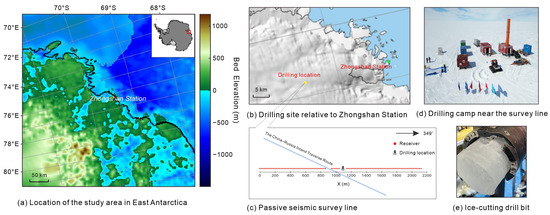
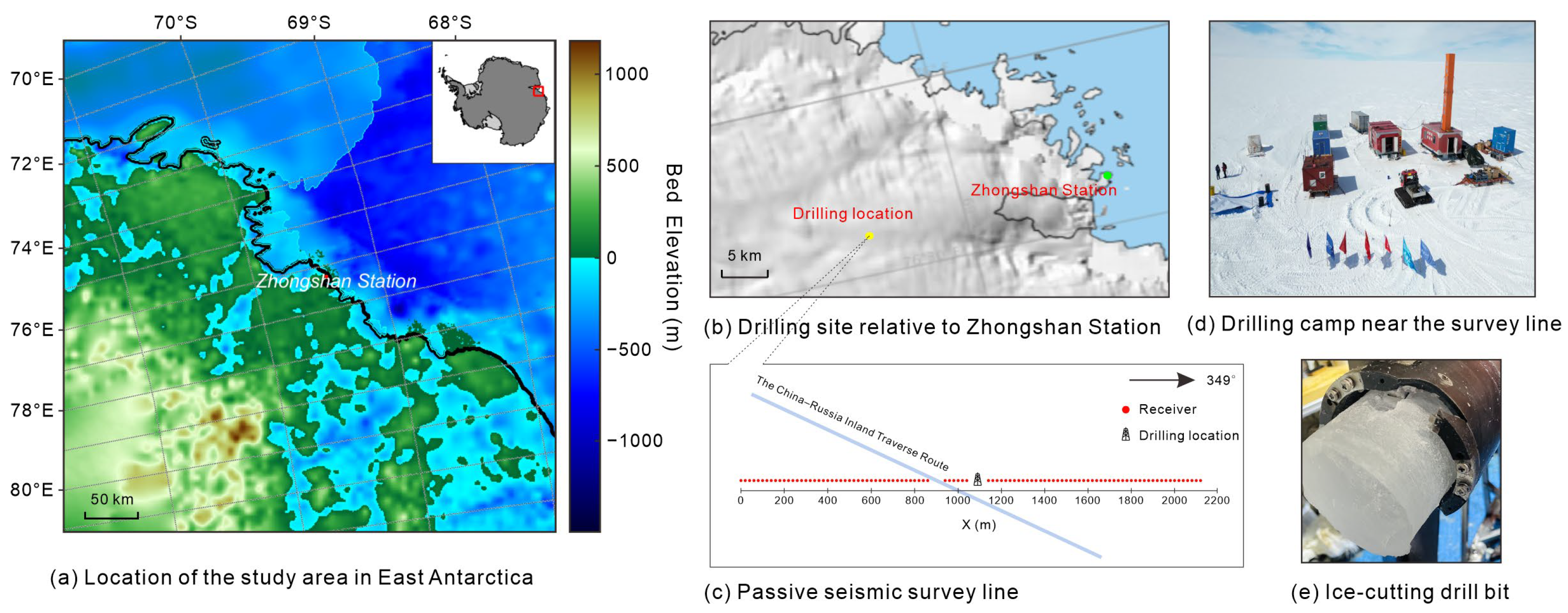
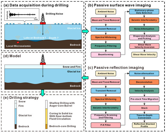
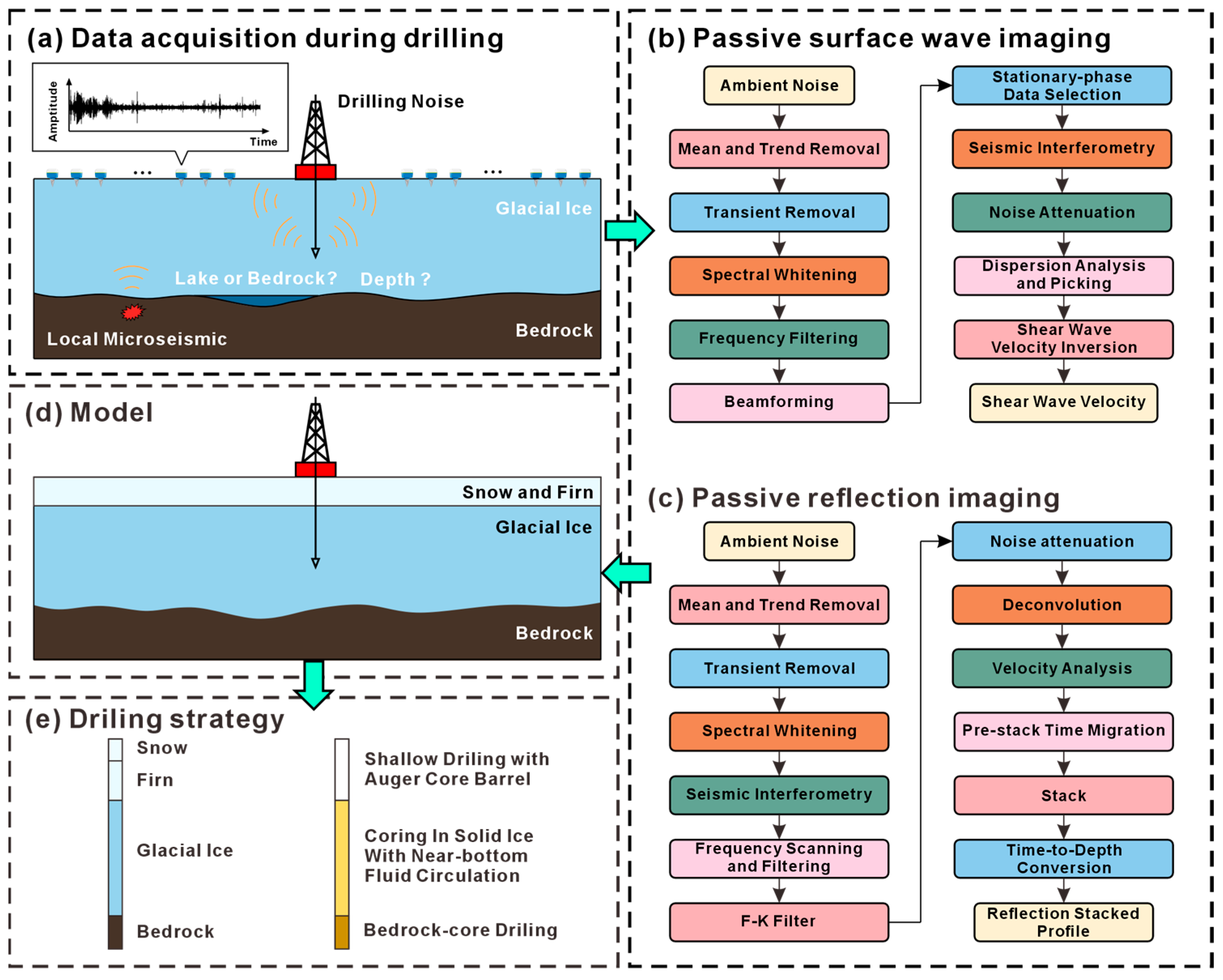
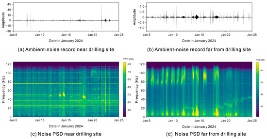
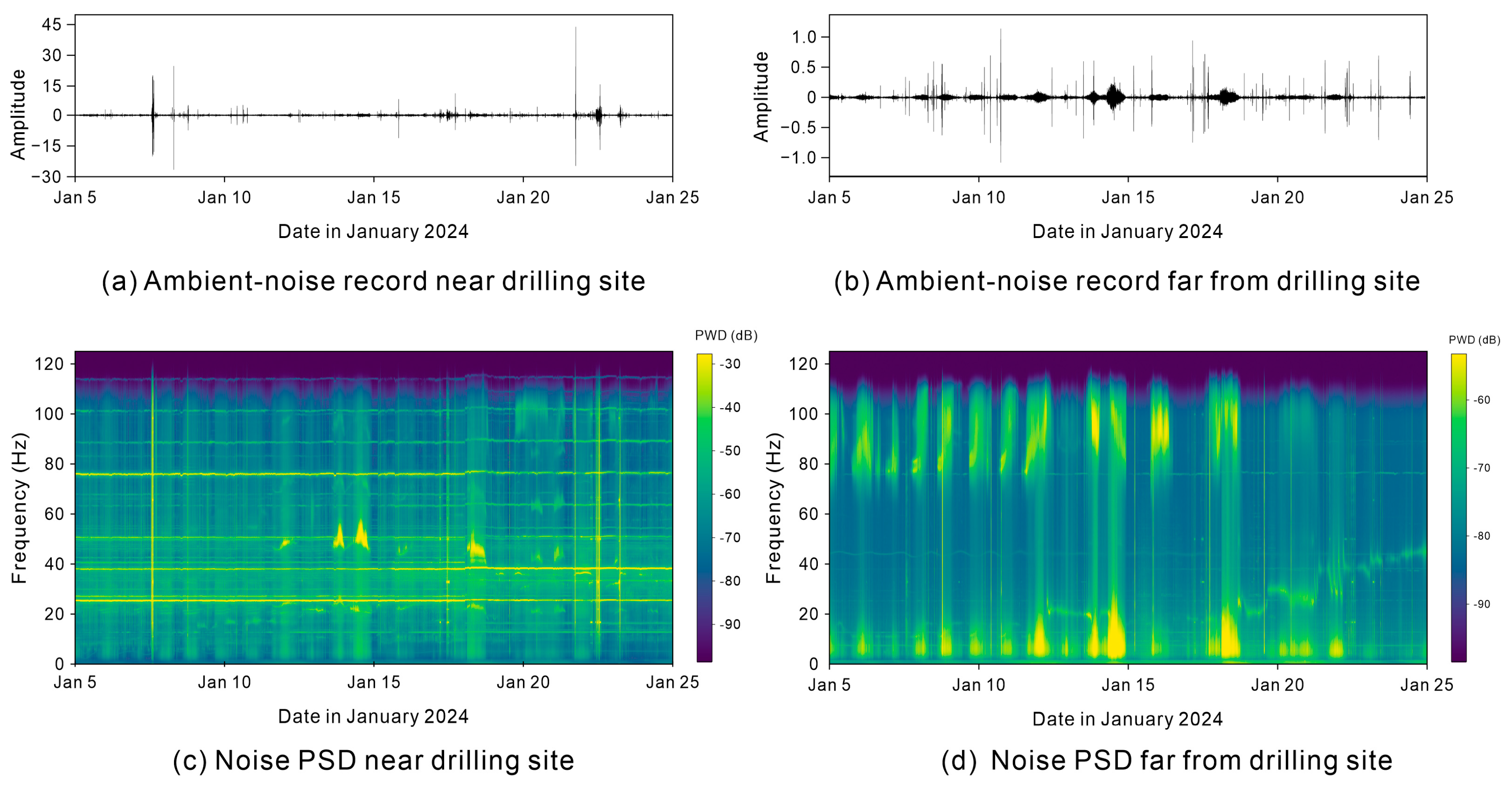
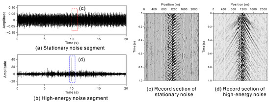
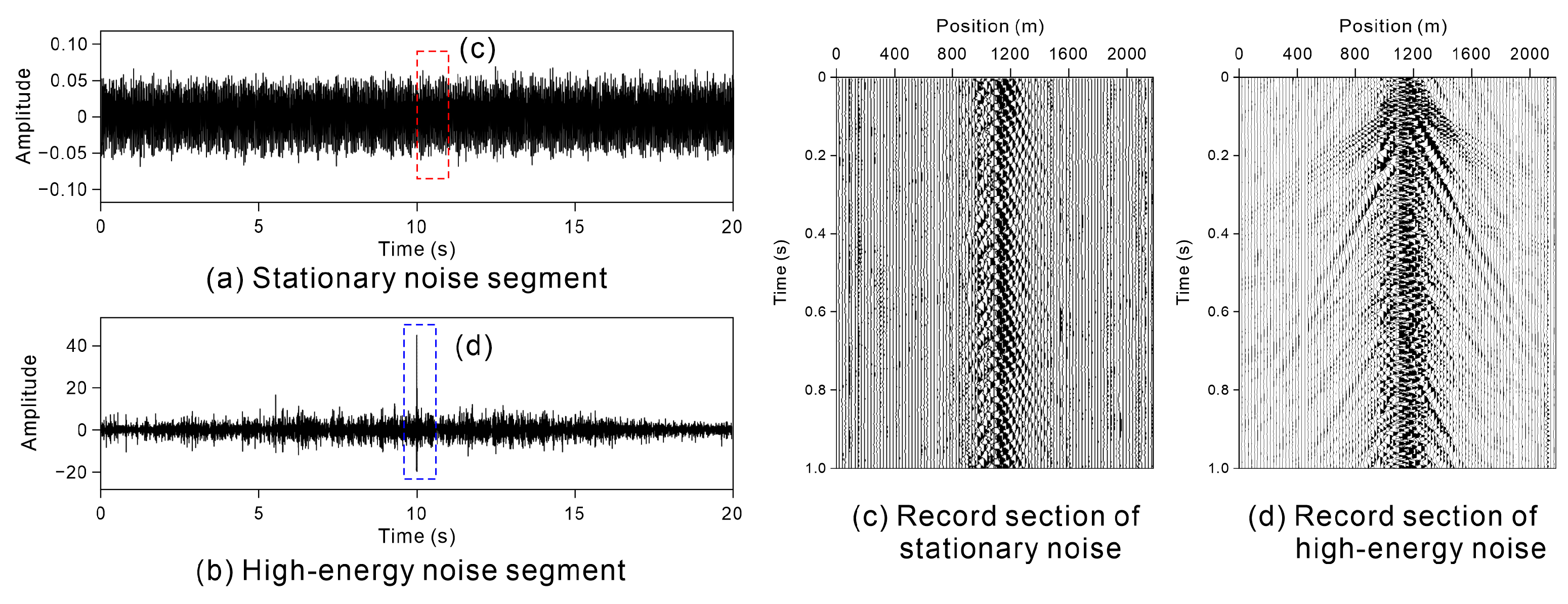
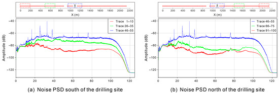
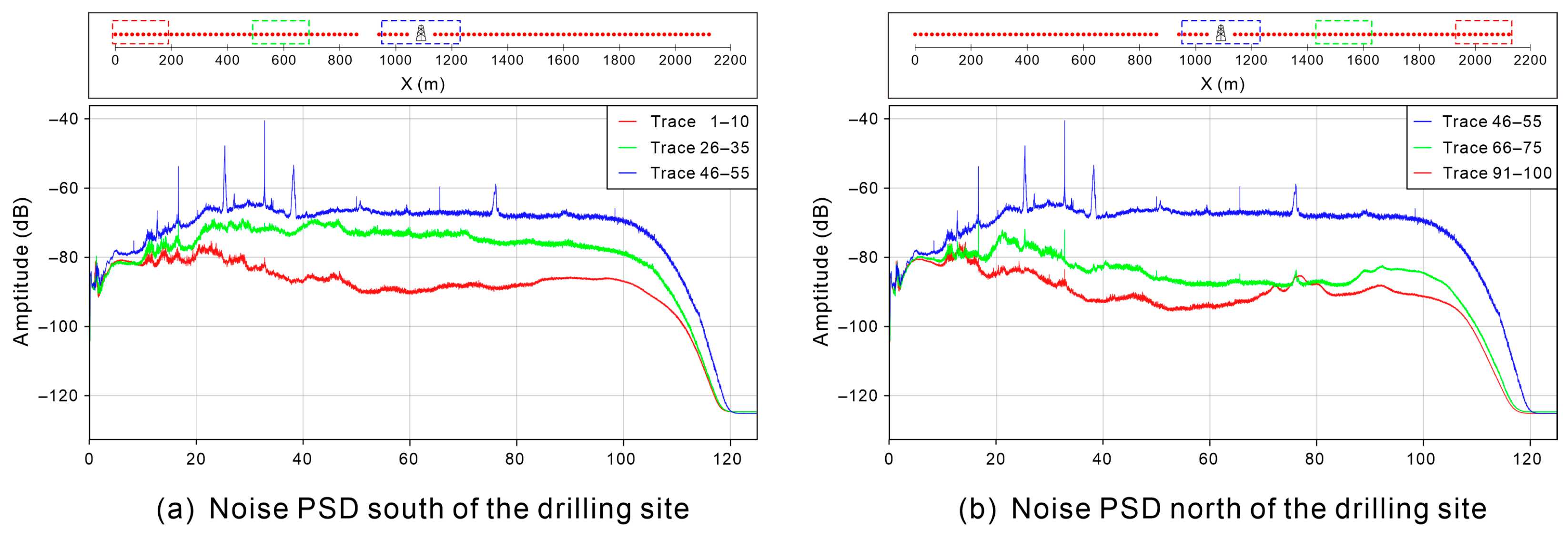
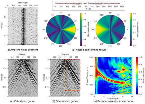
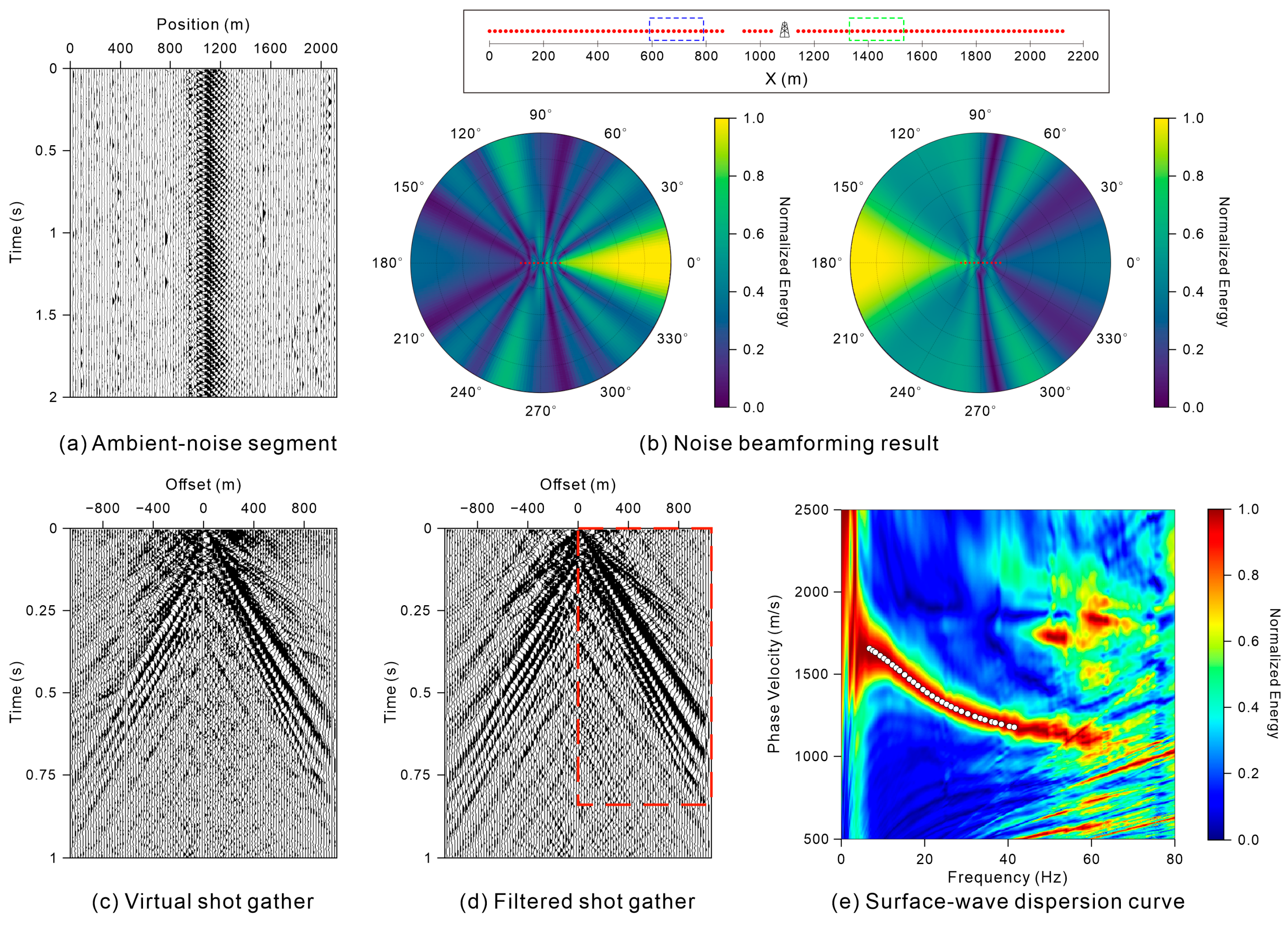
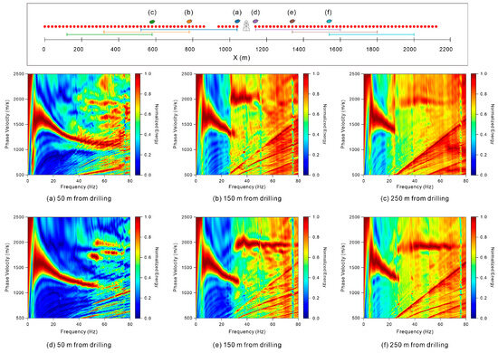
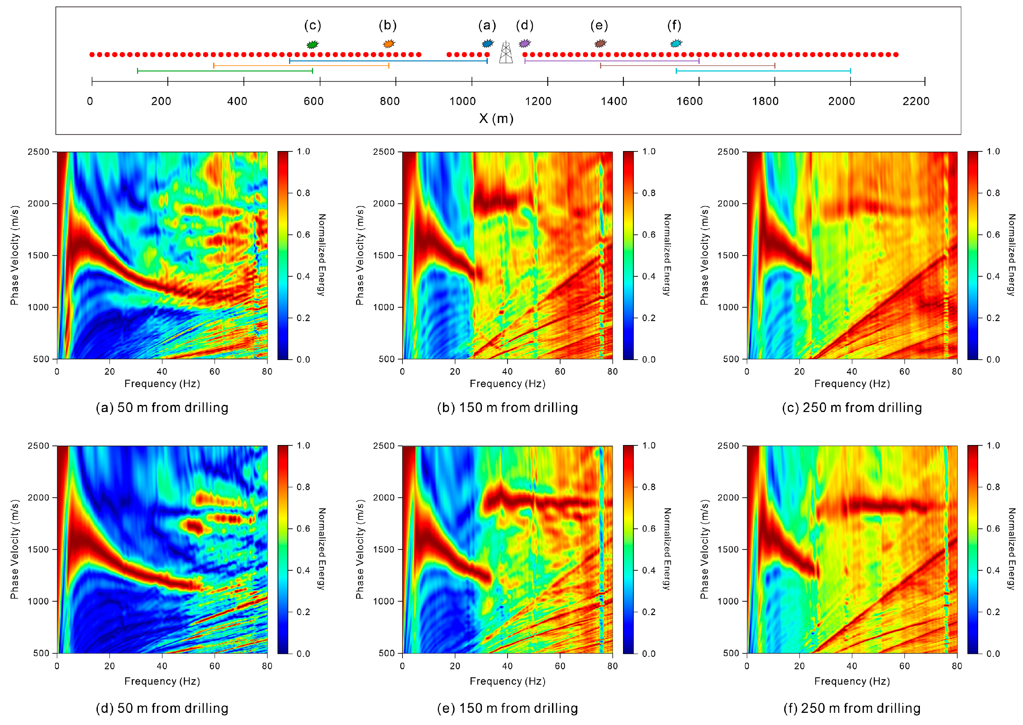
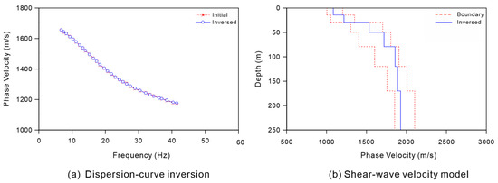
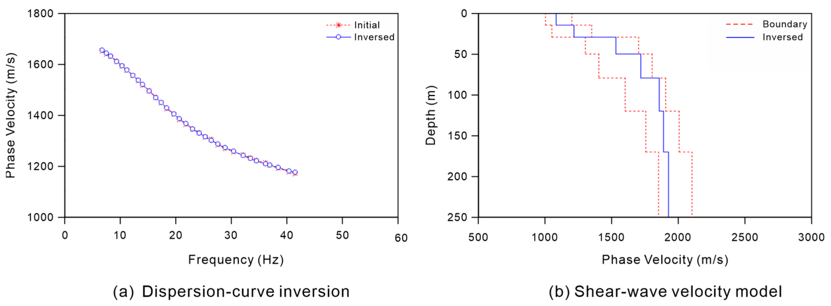
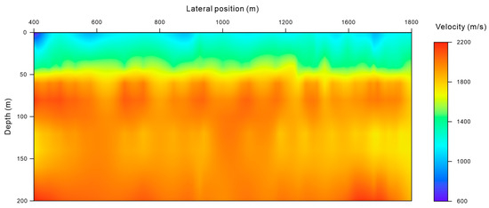
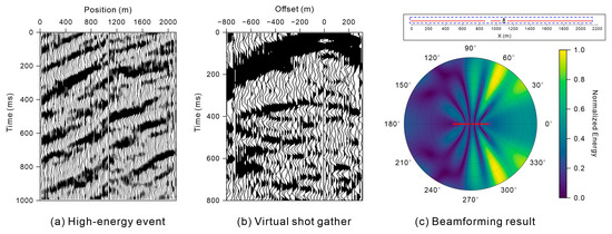
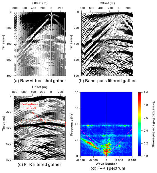
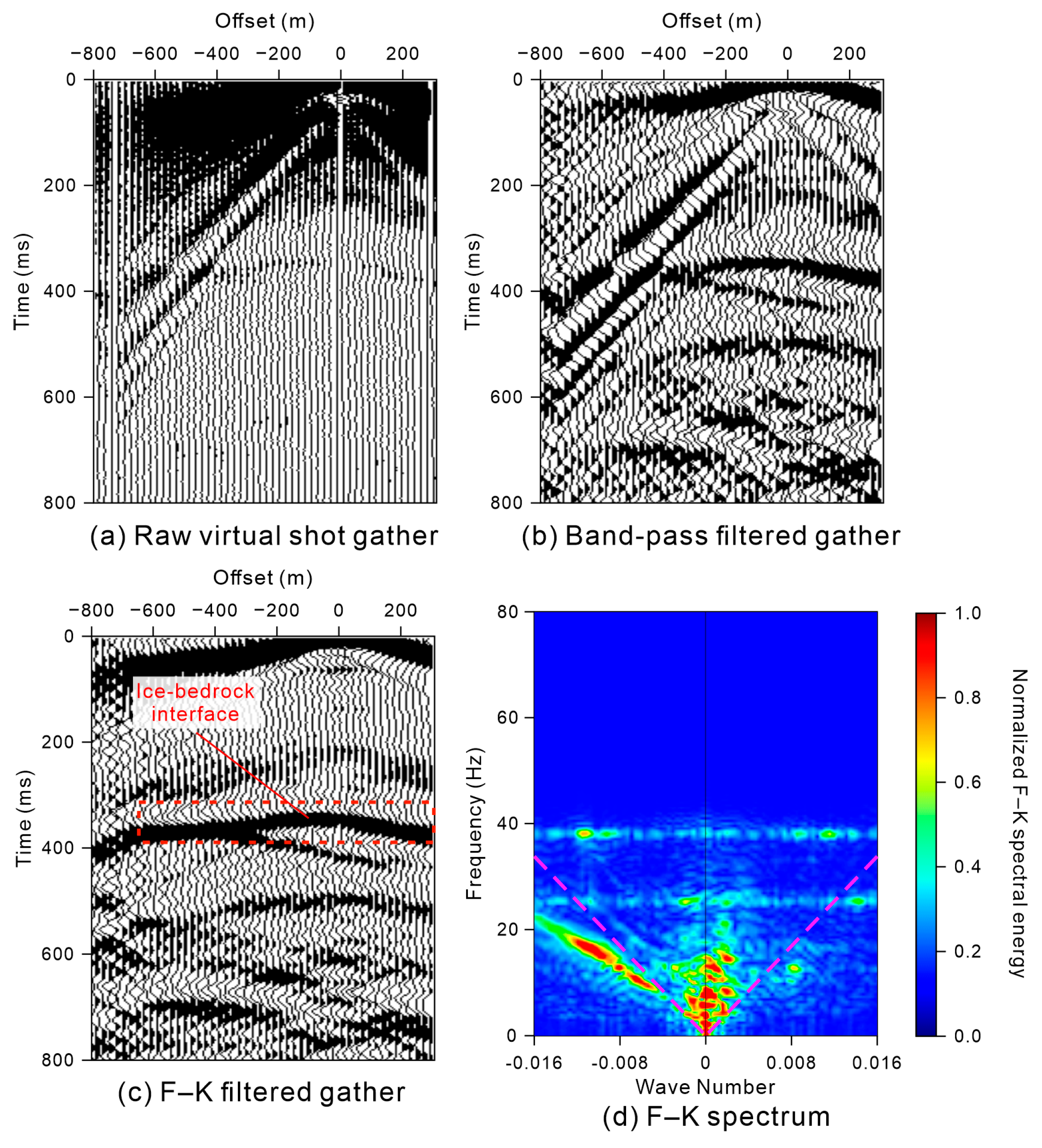
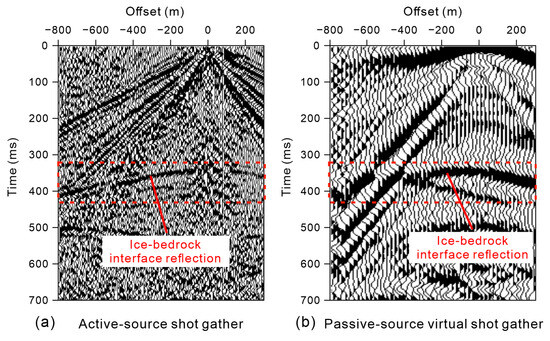
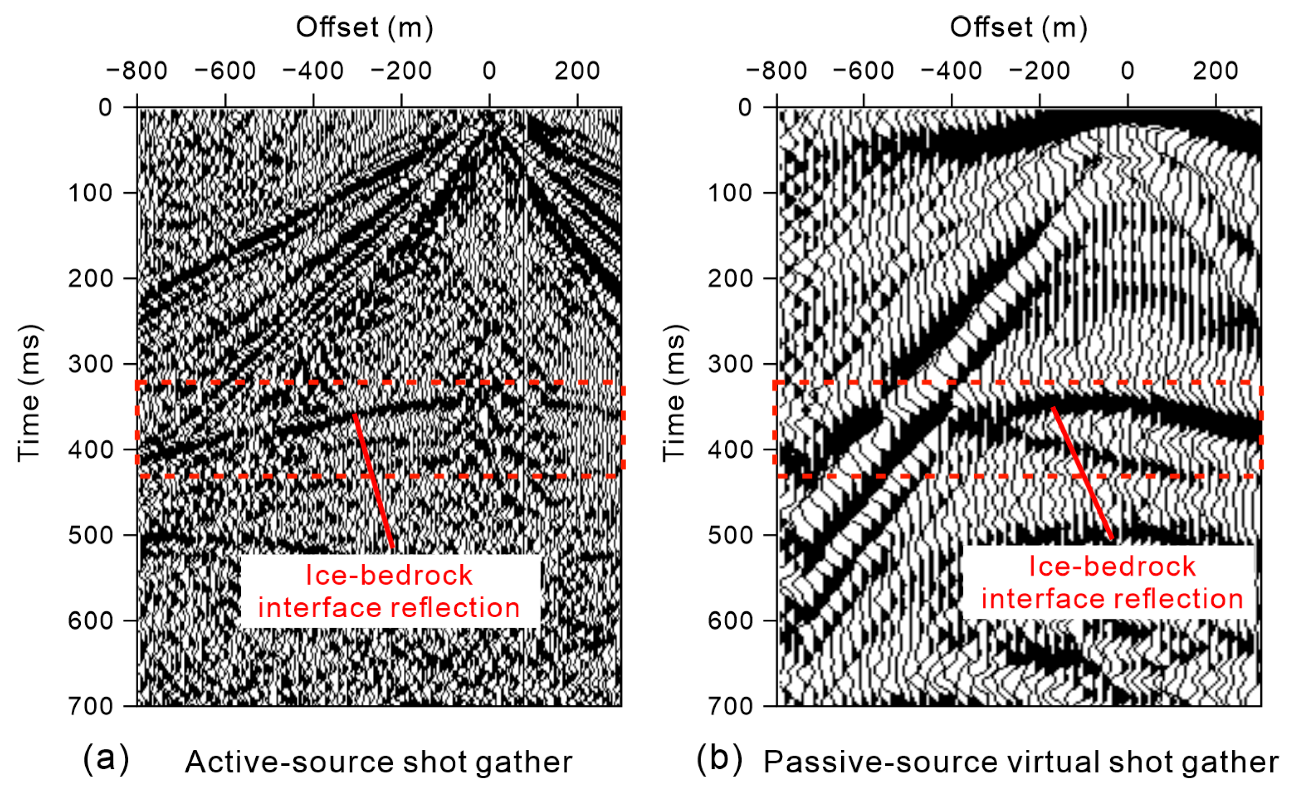
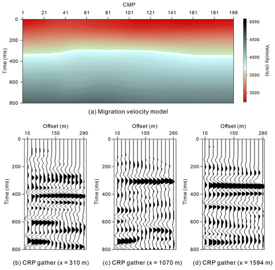
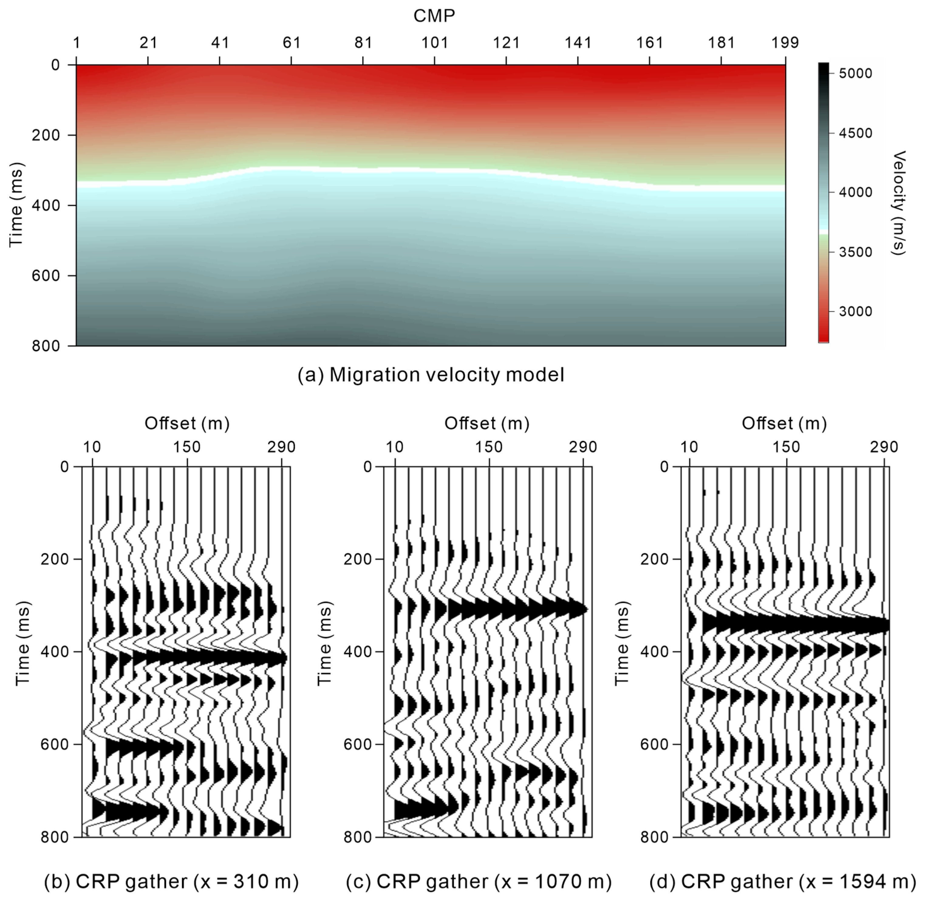
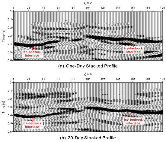
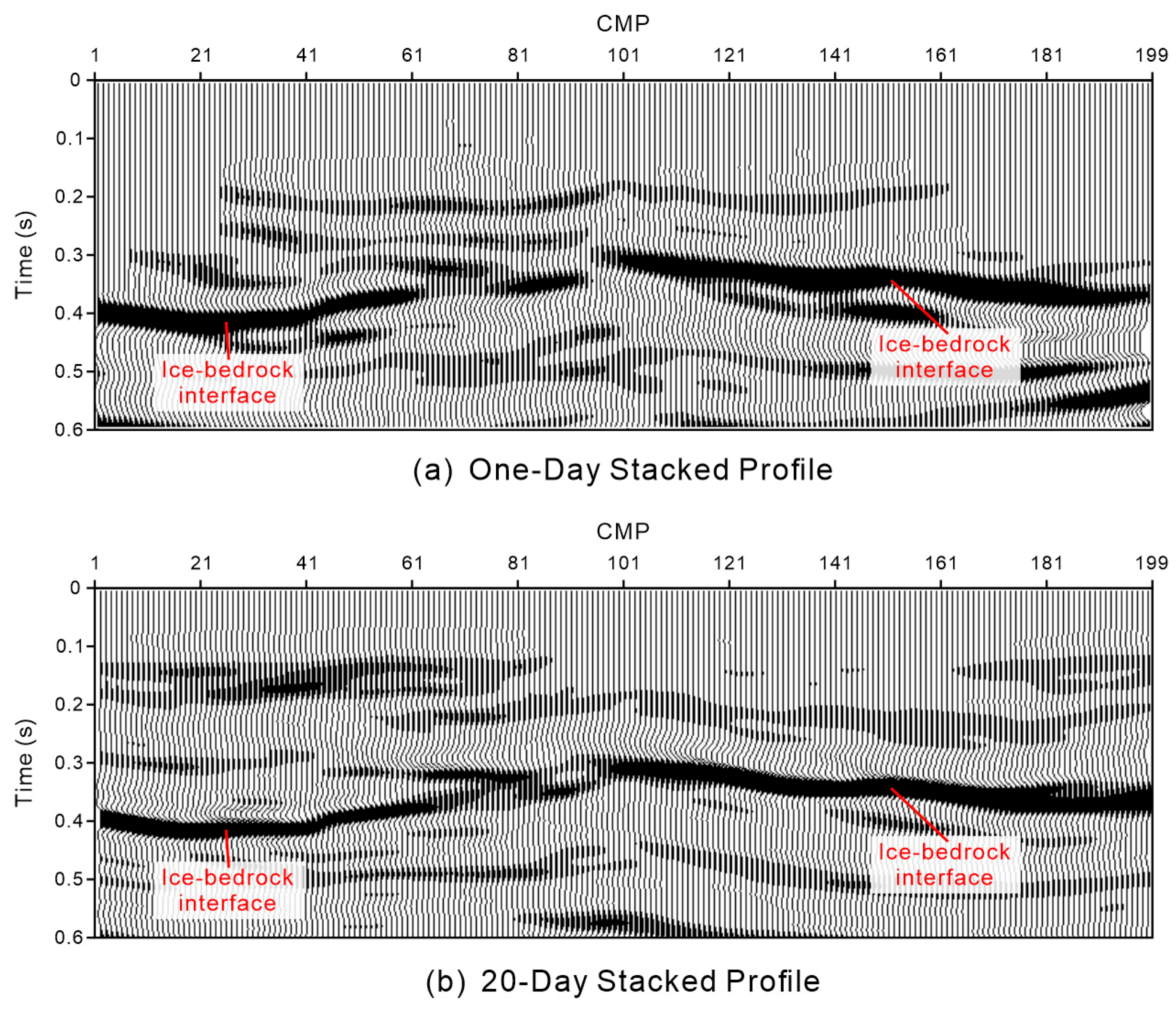
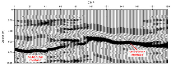
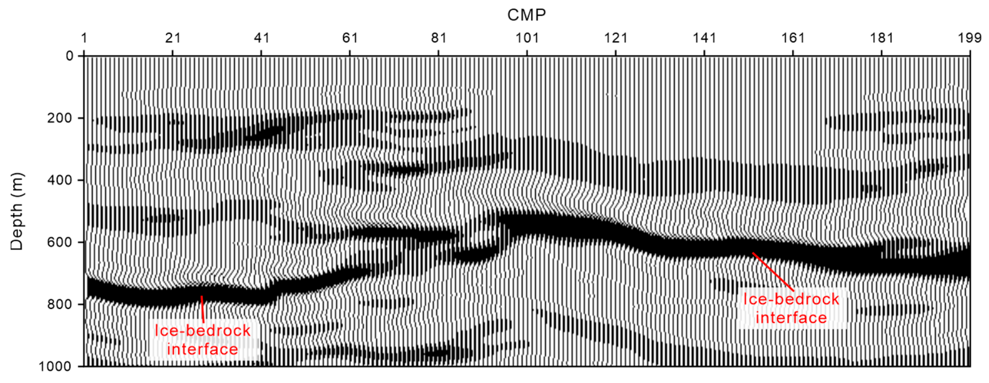
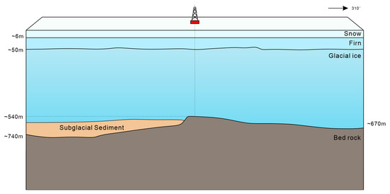
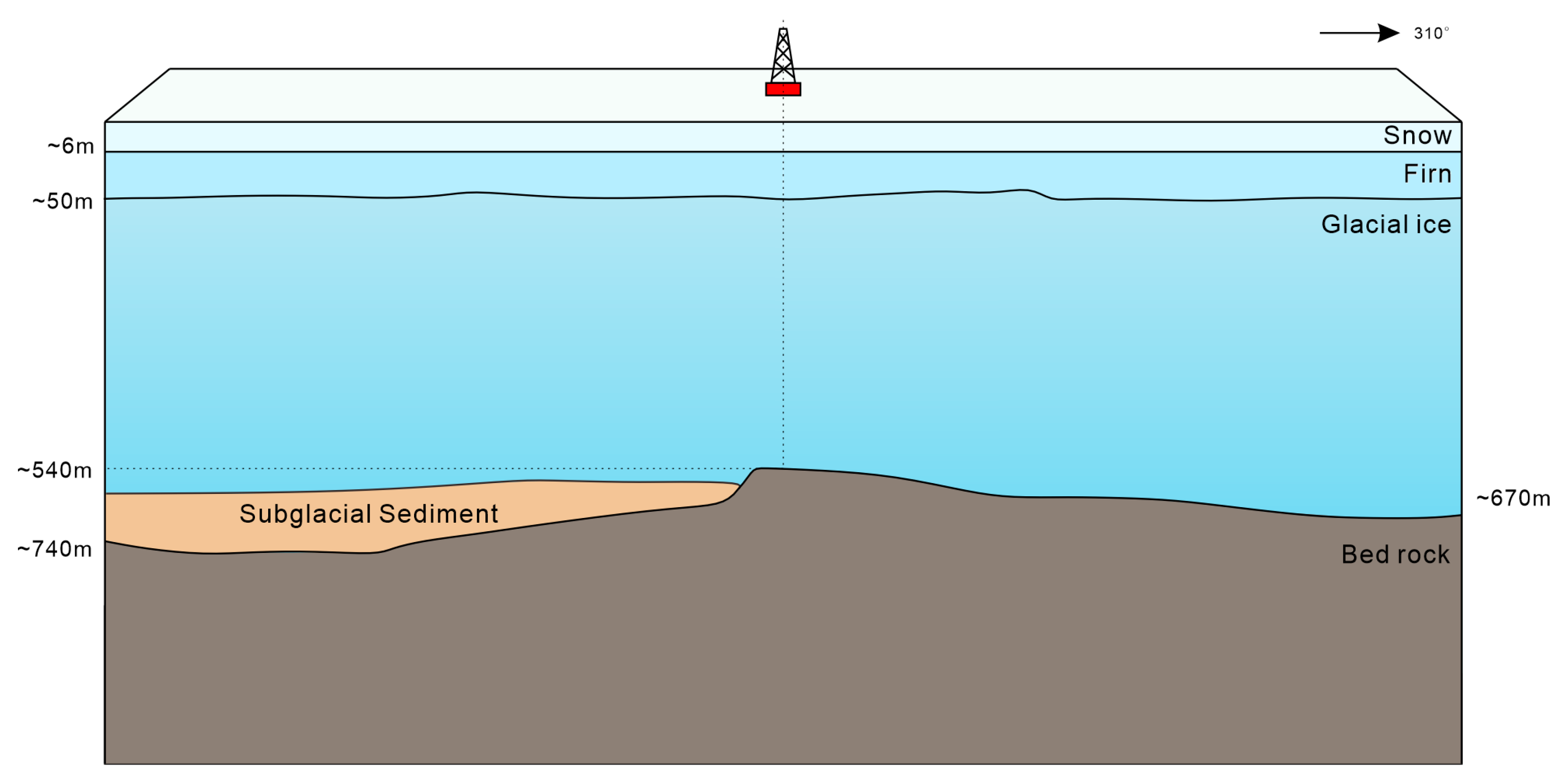
Disclaimer/Publisher’s Note: The statements, opinions and data contained in all publications are solely those of the individual author(s) and contributor(s) and not of MDPI and/or the editor(s). MDPI and/or the editor(s) disclaim responsibility for any injury to people or property resulting from any ideas, methods, instructions or products referred to in the content. |
© 2026 by the authors. Licensee MDPI, Basel, Switzerland. This article is an open access article distributed under the terms and conditions of the Creative Commons Attribution (CC BY) license.