


Highlights
What are the main findings?
- UAV RGB-only orthomosaics and a lightweight Tiny U-Net mapped semi-mangrove shrubs on Jeju Island at ~1 cm resolution.
- The model delineated rare, narrow, fragmented patches with robust performance despite severe class imbalance.
What are the implications of the main findings?
- Spatial extent maps and probability surfaces support conservative delineation, targeted field verification, and iterative inventory refinement.
- This reproducible workflow provides a practical baseline for repeat monitoring on Jeju and is transferable to other rare coastal vegetation targets.
Abstract
Semi-mangrove shrubs are important indicators of change in temperate–subtropical coastal ecotones and provide conservation-relevant habitats in shoreline transition zones. On Jeju Island, South Korea, the distribution of two key semi-mangrove species (Hibiscus hamabo and Paliurus ramosissimus) remains incompletely documented despite their monitoring value. Because these shrubs occur as narrow, fragmented patches that are difficult to delineate in satellite imagery, they may be omitted from coarse-resolution inventories. Here, we produced high-resolution semi-mangrove maps from 1 cm UAV RGB orthomosaics using a lightweight Tiny U-Net semantic segmentation model trained on field-confirmed, expert-digitized polygons from nine coastal sites. Model performance was evaluated using a site-wise training, validation, and test split. The final model achieved a pooled semi-mangrove IoU of 0.677, balanced accuracy of 0.921, precision of 0.771, recall of 0.848, and a false-positive rate of 0.007, despite the low semi-mangrove prevalence of 2.59%. On the independent test site, Tiny U-Net also outperformed standard U-Net with fewer parameters and shorter training time (IoU = 0.873 vs. 0.568; 1.9 M vs. 31.4 M parameters; 37 vs. 123 min). Probability outputs also highlighted high-confidence candidate patches outside of the labeled polygons, supporting targeted field verification and iterative inventory refinement. This UAV–deep learning workflow provides a practical baseline for fine-scale habitat assessment and repeat monitoring of vegetation dynamics along Jeju’s temperate–subtropical coast.
1. Introduction
Mangrove ecosystems provide critical services disproportionate to their areal extent, including shoreline stabilization, nursery habitats, and substantial blue carbon storage in biomass and deep organic soils [1,2,3,4,5]. As climate change drives the poleward expansion of these tropical species, they are projected to encroach upon temperate coastal transition zones [6]. In these transition zones, mangrove communities interact with semi-mangrove (mangrove associate) vegetation, defined here as salt-tolerant trees and shrubs that occupy landward coastal ecotones with less frequent tidal inundation [7]. Consequently, distinguishing and monitoring these resident associates is essential for establishing a spatial baseline against which future range shifts and habitat transitions can be detected [7,8].
Jeju Island, South Korea, situated near the northern limit for various subtropical coastal taxa, serves as a critical sentinel for climate-driven tropicalization of coastal ecosystems [9]. Recent analyses indicate that winter sea surface warming, milder winters, and a reduced frequency of extreme cold events can relax thermal constraints and promote poleward expansion of mangroves [8]. Globally, climate-driven replacement of salt marshes by woody coastal vegetation is well documented [10,11,12,13]. However, spatially explicit baseline maps for Jeju semi-mangrove species, such as Hibiscus hamabo Siebold & Zucc. and Paliurus ramosissimus (Lour.) Poir., remain scarce [14,15]. Despite their rarity and fragmented distribution, these species exhibit high salt tolerance and may contribute to coastal carbon storage [3,16]. This lack of fine-grained distribution data constrains site-level conservation planning and limits the establishment of a high-resolution baseline for detecting future range shifts and evaluating local habitat or carbon-management actions [9,13].
Remote sensing has become an essential tool for monitoring coastal vegetation dynamics across multiple scales [17,18]. While satellite-based approaches have successfully mapped extensive true mangrove forests globally at large scales [19,20], these methods often lack the spatial granularity required for narrow, patchy transition-zone vegetation such as semi-mangrove shrubs [17]. In Jeju coastal environments, semi-mangrove patches are narrow, linear, and fragmented, and many patches may be smaller than, or similar in size to, the effective pixel size of commonly used satellite imagery. As a result, a single satellite pixel can contain a semi-mangrove canopy together with sand, rock, water, shadow, and other coastal vegetation, producing mixed-pixel interference and background confusion [11,21,22]. These effects can cause the omission of small, fragmented patches and commission errors from visually similar background vegetation [22,23,24]. In addition, coarse or moderate spatial resolution reduces boundary delineation accuracy because patch edges can be spatially blurred or merged with surrounding substrates. Addressing these limitations requires a shift from orbital to aerial perspectives. High-resolution Unmanned Aerial Vehicle (UAV) imagery can resolve discrete boundaries and small individuals within salt-tolerant semi-mangrove assemblages [25]. Recent drone-based and fine-resolution mangrove mapping studies have also shown that fine-resolution aerial imagery improves patch-level mapping, preserves fragmented vegetation patches, and better delineates complex coastal boundaries compared with coarser mapping products [26,27].
To fully exploit centimeter-scale UAV imagery, an automatic segmentation framework is required because manual interpretation of large orthomosaics is time-consuming and difficult to repeat consistently. Conventional pixel-based, object-based, and basic machine-learning methods can be limited in heterogeneous coastal environments, where semi-mangrove shrubs occur together with sand, rock, water margins, shadows, and non-target vegetation [28,29,30]. Deep learning methods, especially encoder–decoder architectures such as U-Net, are useful because they learn spatial context as well as local image features for pixel-wise segmentation [31]. However, standard U-Net-type models can be computationally demanding when applied repeatedly to large 1 cm UAV orthomosaics. Therefore, operational coastal monitoring benefits from lightweight architectures that reduce model size and memory demand while retaining skip connections for fine boundary localization [31,32,33]. In addition, semi-mangrove mapping is a rare-class segmentation problem because the target shrubs occupy only a small fraction of the image area. Without imbalance-aware sampling and loss functions, training can be biased toward the dominant background class, causing missed small patches or unstable false detections [24,32,33,34,35,36].
Despite these technological advances, high-resolution, site-validated inventories of semi-mangrove habitats remain scarce, and few studies have tested a lightweight, imbalance-aware UAV RGB workflow for rare and fragmented semi-mangrove shrubs in heterogeneous coastal environments. Therefore, this study aimed to develop a practical UAV RGB-based workflow for fine-scale semi-mangrove mapping by: (1) building expert-labeled centimeter-scale datasets across nine coastal sites on Jeju Island; (2) developing a lightweight Tiny U-Net for pixel-wise semi-mangrove segmentation, addressing severe class imbalance; and (3) producing map and probability outputs that support field verification and iterative inventory refinement. By assembling expert-digitized labels in complex coastal environments, this study provides a fine-scale baseline for semi-mangrove monitoring on Jeju Island and a practical workflow that can be adapted for other rare and patchy coastal vegetation targets.
2. Materials and Methods
2.1. Study Domain and Target Species
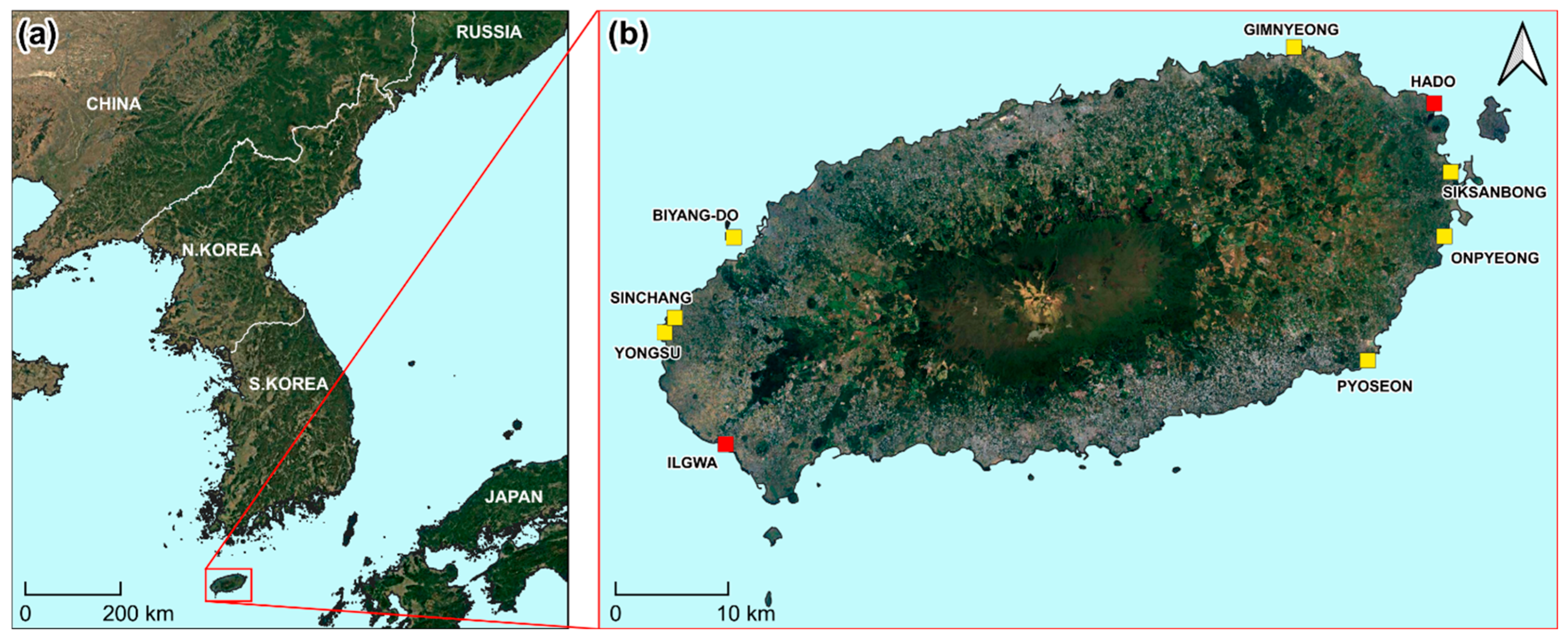
Jeju Island (≈33°N, 126°E) is located off the southern margin of the Korean Peninsula (Figure 1a) within a temperate–subtropical transition zone where warm currents (Kuroshio-derived waters and the Tsushima Warm Current) and frequent typhoon disturbance shape nearshore conditions [37]. Along Jeju’s shoreline, coastal sand-dune and rocky and gravelly coastal ecotones support specialized plant communities under high development pressure, providing habitat for fragmented patches of coastal shrubs, including Hibiscus hamabo (H. hamabo) and Paliurus ramosissimus (P. ramosissimus) [16,38].
Figure 1.
Study area and UAV survey sites on Jeju Island, South Korea. (a) Jeju Island in relation to the Korean Peninsula. (b) Locations of the surveyed semi-mangrove sites. Training sites are indicated in yellow (n = 7), and the validation (Ilgwa) and test (Hado) sites are indicated in red.
The nine UAV survey sites covered different coastal backgrounds, including rocky or tidal shorelines, wet areas, dense vegetation, roads, footpaths, and human-disturbed areas (Figure 1b and Table 1). Ilgwa and Hado were used as independent sites because of their distinct shoreline background and mapping challenges. This site-wise split reduced spatial leakage and allowed model evaluation on unseen coastal locations. UAV imagery from all sites was processed into high-resolution orthomosaics for subsequent analysis (Section 2.2.1).
Table 1.
Habitat and background characteristics and main mapping challenges of the UAV survey sites.
2.2. Data Acquisition
2.2.1. Drone Imagery
We acquired nadir images at nine coastal sites using a DJI Phantom 4 Pro UAV (Shenzhen, China) equipped with its built-in optical RGB camera. Flights were conducted at approximately 45–50 m above ground level in July 2023. The flights were planned with high front and side overlap to generate high-resolution RGB orthomosaics. The final GeoTIFF orthomosaics were checked in QGIS (version 3.34) and confirmed to have a pixel size of 0.01 m × 0.01 m, corresponding to a 1 cm ground sample distance (GSD). Drone images were processed to generate one orthomosaic and one digital surface model for each site. The resulting orthomosaics were visually inspected for seamline artifacts and georegistration errors before model training and evaluation. Flight overlap and speed were set in the UAV mission plan and adjusted slightly according to site geometry and flight safety conditions.
2.2.2. Field Verification and Ground Truth
Before manual annotation, trained researchers conducted field-based vegetation surveys at all nine sites to verify the presence and location of the target semi-mangrove species. During the field survey, the locations of H. hamabo and P. ramosissimus patches were recorded using GPS. These field-confirmed records were used as the primary reference for identifying target vegetation in the UAV orthomosaic images.
Ground-truth labels were prepared by manually digitizing semi-mangrove polygons on the 1 cm UAV RGB orthomosaics in QGIS (version 3.34). The labeling criteria were based on field-confirmed, expert-based visual interpretation rather than numerical spectral or color thresholds. In the orthomosaic images, H. hamabo and P. ramosissimus were visually distinguished from surrounding vegetation using canopy color, texture, patch shape, and GPS-recorded field locations. Patch boundaries were delineated along the visible canopy edge where the target vegetation could be separated from adjacent vegetation, exposed rock, water, bare ground, roads, or other surrounding surfaces.
During field verification and manual digitization, H. hamabo and P. ramosissimus were identified separately where possible. However, for model training and evaluation, the two species were merged into one binary semi-mangrove class because the objective of this study was to map total semi-mangrove shrub extent, and species-level samples were sparse and unevenly distributed across sites.
To reduce potential subjective errors, the digitized polygons were cross-checked against field survey records, GPS points, and UAV orthomosaic images. Ambiguous boundaries were reviewed and corrected before finalizing the reference data. The final polygons were rasterized to the orthomosaic grid at native resolution to generate pixel-aligned binary masks for model training and evaluation. This alignment is critical because small spatial offsets between imagery and labels can introduce systematic boundary errors during training and evaluation [25].
2.3. Model Development
2.3.1. Model Workflow
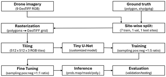
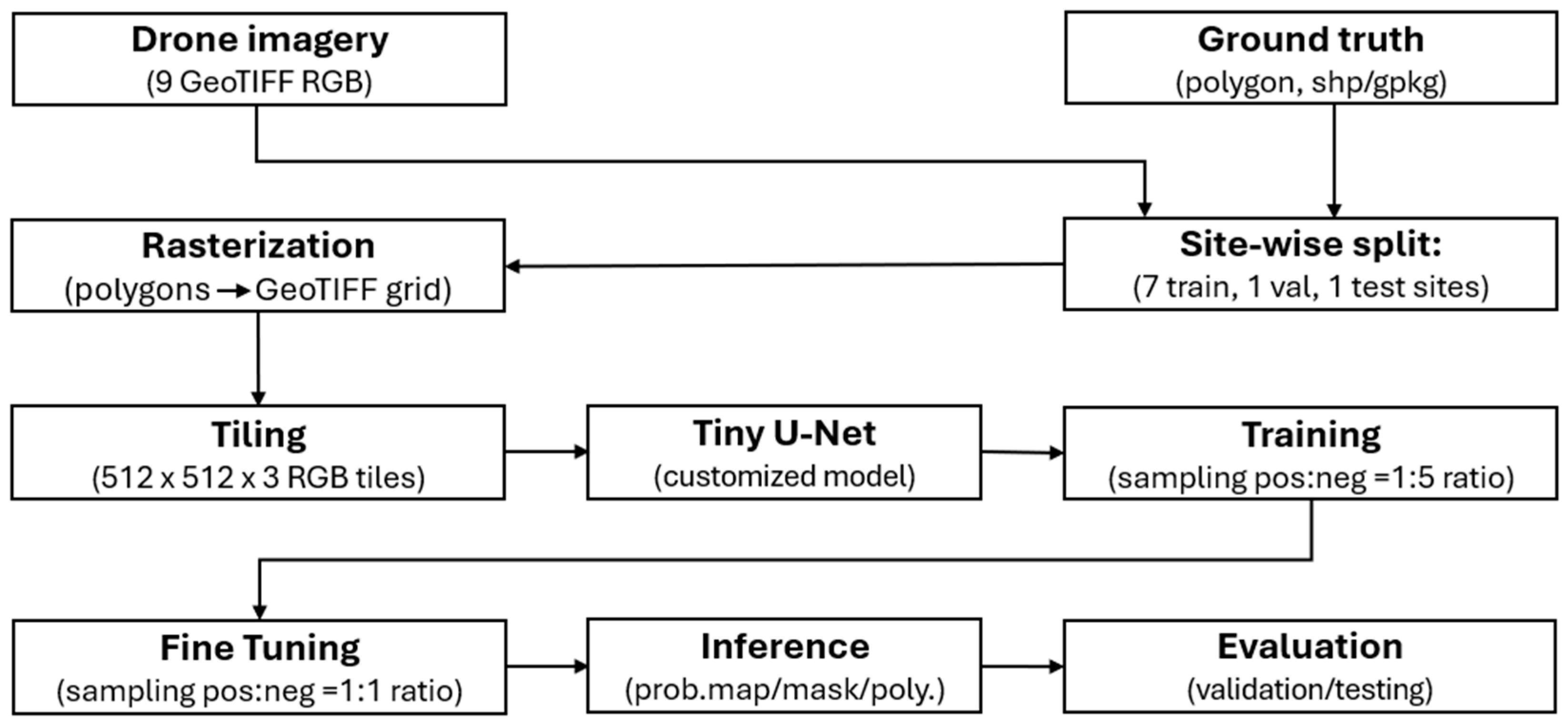
Figure 2 outlines the model-development workflow used to generate pixel-wise semi-mangrove maps from centimeter-scale drone imagery. First, the orthomosaics and rasterized labels were tiled into fixed-size RGB patches using an overlapping sliding window, enabling efficient GPU training on large scenes and mitigating edge effects common in high-resolution segmentation [29,32]. To prevent spatial leakage, we applied a site-wise split: Hado was reserved for independent testing, Ilgwa for validation, and the remaining sites for training (i.e., 7 for training, 1 for validation, and 1 for test). Using this split, a customized Tiny U-Net [31] was trained to predict per-pixel semi-mangrove probabilities, which were converted to binary masks and vector polygons for mapping and analysis. Given the sparsity of semi-mangrove pixels, we incorporated imbalance-aware sampling and loss functions during training and evaluated performance on the validation and test sites using standard segmentation metrics and visual inspection. Implementation details are provided in the remainder of the Methods section.
Figure 2.
Semi-mangrove mapping workflow using UAV RGB orthomosaics and polygon labels. Sites were split into training (7), validation (1), and test (1). Polygon labels were rasterized and imagery was tiled into 512 × 512-pixel patches. A Tiny U-Net was trained using a positive-to-negative patch sampling ratio of 1:5, followed by 1:1 fine-tuning. Outputs (probability maps, binary masks, and vector polygons) were evaluated on the validation and test sites.
2.3.2. Tiny U-Net Architecture
We designed a compact encoder–decoder segmentation network (“Tiny U-Net”) derived from the standard U-Net architecture [31]. The motivation for a lightweight design is threefold. First, UAV orthophoto datasets at 1 cm GSD are typically small in tile count compared with natural-image benchmarks, and deeper networks with tens of millions of parameters are at greater risk of overfitting on such limited training corpora. Second, practical deployment of UAV-based mangrove mapping pipelines benefits from low memory and computational requirements so that training and inference can be performed on a single mid-range GPU and the trained model can be embedded into field workstations. Third, at 1 cm GSD, the spatial features that distinguish semi-mangrove vegetation from surrounding land cover, including individual canopies, branch shadows, and narrow strips of vegetation along shorelines, are resolved within a few tens of pixels, so a moderate receptive field is sufficient and additional depth yields diminishing returns relative to the increase in parameter count and training time [26,27,31].
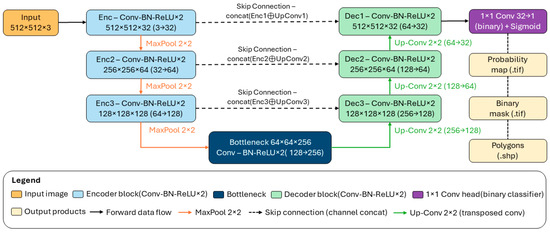
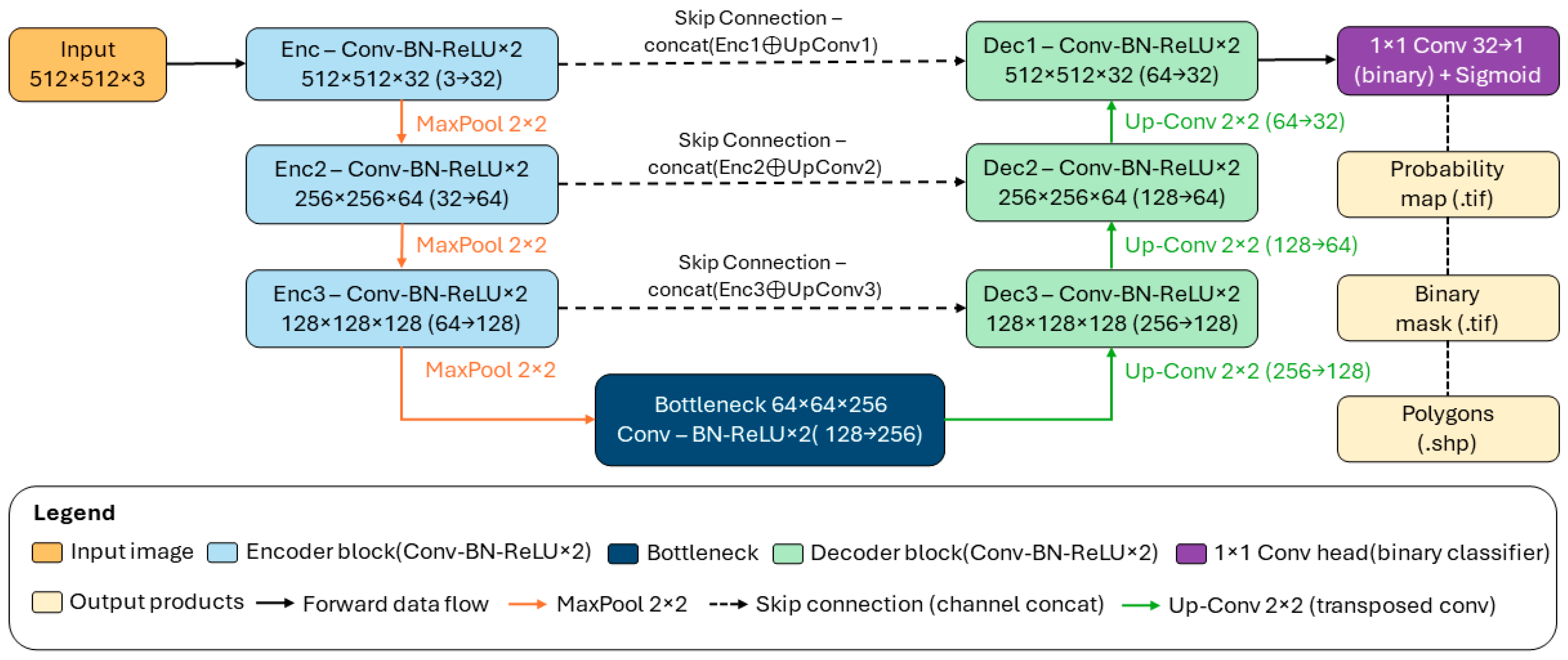
The proposed architecture (Figure 3) operates on 512 × 512 × 3 RGB tiles extracted from the 1 cm GSD orthomosaics and consists of three encoder levels, one bottleneck level, and three corresponding decoder levels. Each block is implemented as two successive 3 × 3 padded (“same”) convolutions, each followed by Batch Normalization (BN) and a Rectified Linear Unit (ReLU) activation; we denote this as a Conv–BN–ReLU block. BN is applied throughout to stabilize training under mixed-precision optimization, in contrast to the original U-Net of [31], which predates the widespread adoption of BN.
Figure 3.
Tiny U-Net architecture for pixel-wise semi-mangrove segmentation from UAV RGB orthomosaics. The four-level encoder–decoder (spatial resolutions 512 → 256 → 128 → 64; channel counts 32—64—128—256) consists of paired Conv—BatchNorm—ReLU blocks, 2 × 2 max-pooling for down-sampling, 2 × 2 transposed convolutions for up-sampling, and skip connections with feature concatenation between corresponding encoder and decoder levels. A final 1 × 1 convolution with sigmoid activation produces per-pixel semi-mangrove probabilities, which are thresholded and post-processed into binary masks, then polygonised into vector outputs (Shapefile).
The encoder path progressively halves spatial resolution while doubling feature depth. The first encoder block (Enc1) maps the 512 × 512 × 3 input to a 512 × 512 × 32 feature map. A 2 × 2 max-pooling layer then halves the spatial resolution, after which the second block (Enc2) produces a 256 × 256 × 64 representation. A further pooling and third block (Enc3) yield a 128 × 128 × 128 feature map. A final pooling step is followed by the bottleneck block, which outputs a 64 × 64 × 256 representation that captures tile-level contextual information.
The decoder path mirrors the encoder with three up-sampling stages. Each stage begins with a 2 × 2 transposed convolution that doubles spatial resolution and halves channel depth. The up-sampled feature map is concatenated with the corresponding encoder feature map of the same spatial size via a skip connection, restoring high-frequency spatial detail lost during pooling and improving boundary localization, following the standard U-Net design [31]. Two further Conv–BN–ReLU operations after each concatenation fuse encoder and decoder features, producing decoder feature maps of size 128 × 128 × 128 (Dec3), 256 × 256 × 64 (Dec2), and 512 × 512 × 32 (Dec1). A final 1 × 1 convolution projects the 32-channel Dec1 output to a single per-pixel logit, to which a sigmoid activation is applied to obtain semi-mangrove probabilities. The probability map is thresholded at an operating point selected by a validation sweep over the interval [0.3, 0.7] (Section 2.3.3) to produce a binary mask, which is morphologically post-processed (small-object and small-hole removal with a 2000-pixel area threshold) and converted to vector polygons in Shapefile format for downstream spatial analysis.
2.3.3. Training Configuration and Implementation Details
We trained the Tiny U-Net using images from seven training sites (Figure 1b). Each orthomosaic was tiled into 512 × 512-pixel RGB patches with 50% overlap (stride = 256 pixels). RGB values were normalized to [0, 1] using min–max scaling per tile. Given the strong class imbalance in semi-mangrove coverage, we employed tile-level sampling based on the fraction of semi-mangrove pixels in each label mask:
where is the positive-pixel fraction and is the number of semi-mangrove pixels in a 512 × 512 tile.
A tile was treated as positive if was greater than 0.20 to select tiles containing a sufficient amount of semi-mangrove canopy while avoiding tiles with only a few boundary pixels or isolated label noise. This helped define positive training tiles with meaningful target information, while background-dominant tiles were kept as negative samples. In the initial training stage, we compared positive:negative tile sampling ratios of 1:0, 1:3, and 1:5 while holding the network architecture, optimizer settings, loss weights, and tiling procedure constant; all models were trained with the same early-stopping criterion on the validation site. The 1:5 stage was used to expose the model to more background variation, including rocks, water, shadows, and non-target vegetation, so that false-positive responses could be reduced. The later 1:1 fine-tuning stage was used to increase the relative contribution of rare semi-mangrove samples after the model had already learned broad background variability.
The network was optimized using Adam (learning rate = 1 × 10⁻³; batch size = 8) for up to 50 epochs with early stopping (patience = 10), using validation mean IoU (mIoU) computed at a probability threshold of 0.5. The final binarization threshold was selected by sweeping {0.3, 0.4, 0.5, 0.6, 0.7} on the validation site and then applying the best threshold to the test site. The training objective was a weighted composite loss combining binary cross-entropy (BCE), focal loss (γ = 2) [24], and Tversky loss (α = 0.6, β = 0.4) [34]. The composite loss weights were chosen to keep BCE and Tversky loss as the main terms, while using focal loss as an auxiliary term for hard-pixel emphasis. The component weights (0.4/0.2/0.4) were selected empirically on the validation set and then fixed for all experiments:
where focal loss emphasizes hard pixels and Tversky loss mitigates class imbalance by reweighting false positives and false negatives.
We used focal loss and Tversky loss because both are explicitly designed for highly imbalanced segmentation: focal loss down-weights easy background negatives, while Tversky loss allows control over the false-positive and false-negative trade-off, improving precision–recall behavior for rare classes [24,34,35,36]. Predicted masks were post-processed by removing connected components smaller than 2000 pixels and filling holes smaller than 2000 pixels. At the 1 cm GSD, this threshold corresponds to approximately 0.20 m2. The threshold was used to remove isolated noisy predictions and small spurious components while retaining shrub patches large enough for field verification. Because very small, fragmented patches may be removed by this step, the continuous probability maps were retained and used to support visual review and field-verification planning. All experiments used a fixed random seed of 42.
2.4. Inference and Evaluation
Using the trained Tiny U-Net, we performed tiled inference on each orthomosaic and quantified performance against rasterized ground truth. For each orthomosaic, the trained model was applied to overlapping 512 × 512 tiles. Tile-level probability outputs were merged back into a continuous probability surface by averaging probabilities in overlapping regions, reducing seam artifacts typical of tiled inference in high-resolution segmentation [29,39]. The merged probability raster was then thresholded using the validation-selected threshold (Section 2.3.3) to generate a binary semi-mangrove mask.
Quantitative performance was computed by comparing the predicted binary mask with rasterized ground truth at the pixel level. From the confusion matrix, we calculated overall accuracy, precision, recall, F1-score, IoU, specificity, false-positive rate (FPR), false-negative rate (FNR), negative predictive value, balanced accuracy, and predicted positive fraction, which are commonly used to evaluate semantic segmentation and class-imbalanced classification performance [20,33,35,36,40]. Because semi-mangrove pixels occupied only a small fraction of the evaluated area, overall accuracy was interpreted with caution, and class-specific and imbalance-aware metrics were emphasized [35,36]. To support interpretation, we also inspected visual overlays and probability maps to identify common error patterns, such as false positives in visually similar vegetation or wet, dark substrates and omissions along shadowed, sparse, or fragmented patch boundaries [25]. Because separate ground-truth labels for error-source classes were not prepared, these error patterns were treated as qualitative observations rather than statistical error-type classes.
2.5. Baseline Comparison with Standard U-Net and Computational Environment
To support the baseline comparison (in Section 3.3), we implemented a standard U-Net baseline as a reference architecture for evaluating the accuracy–efficiency tradeoff of the proposed Tiny U-Net. The standard U-Net was selected because it represents the conventional encoder–decoder segmentation architecture from which Tiny U-Net was derived. For a fair comparison, both models used the same site-wise split, input data, rasterized labels, tile size, stride, normalization, optimizer, learning rate, sampling strategy, composite loss function, threshold-selection procedure, tiled inference, overlap averaging, post-processing, and evaluation metrics. The standard U-Net baseline was adopted for this study: it followed the conventional encoder–decoder structure of the original proposal [31] but was modified for 512 × 512 UAV RGB tiles and pixel-aligned binary probability-map outputs.
Both Tiny U-Net and standard U-Net were trained on the Boston University Shared Computing Cluster using an NVIDIA A100 80 GB PCIe GPU, 8 CPU cores, and 32 GB RAM. Experiments were implemented in Python 3.10.12 using PyTorch 2.1.2+cu118 and CUDA 11.8 in a Linux x86_64 environment. Training time was measured under the same hardware and software environment for both models. Detailed baseline architecture (Figure A1) and computing settings (Table A1) are provided in Appendix A.
3. Results
3.1. Effect of Sampling Ratio on Model Performance
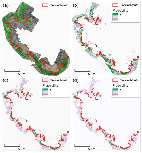
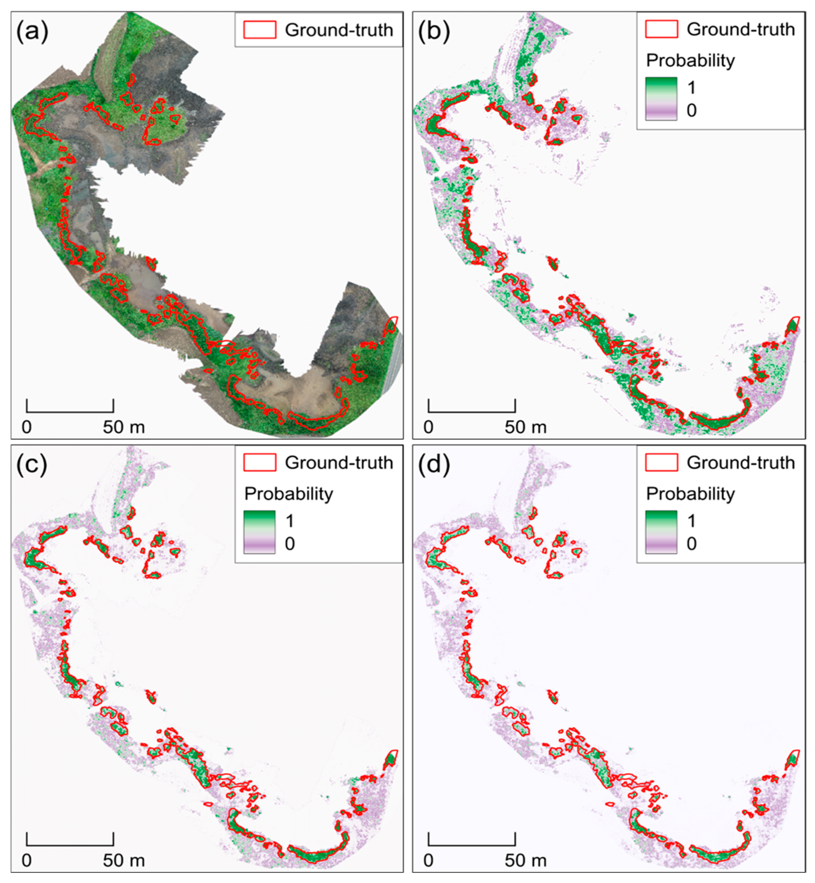
To assess whether class-imbalance handling during training affects segmentation outcomes, we compared semi-mangrove probability maps generated using different positive:negative tile sampling ratios during the initial training stage. The three initial-stage settings, positive-only sampling 1:0, 1:3, and 1:5, were evaluated on both the Ilgwa validation site and the Hado test site using class-specific and imbalance-aware metrics (Table 2).
Table 2.
Validation and testing performance of initial-stage models trained with different sampling ratios.
On the Ilgwa validation site, the 1:5 configuration achieved the highest IoU and F1-score among the evaluated settings, while also reducing FPR, predicted positive fraction, and false-positive area compared with the more positive-heavy sampling ratios. This indicates that including more background-dominant tiles during the initial training stage helped suppress false-positive responses in heterogeneous coastal backgrounds.
Figure 4a shows the Hado RGB orthomosaic used as the visual reference for comparing the probability maps generated by the different sampling ratios. A similar pattern was observed on the Hado test site. The 1:5 configuration achieved the best performance among the evaluated settings (IoU = 0.565, precision = 0.681, recall = 0.767, F1-score = 0.721) and produced the lowest false-positive area. In contrast, the 1:0 and 1:3 settings showed higher recall but lower precision and larger false-positive areas, indicating stronger overprediction of semi-mangrove pixels. The probability maps also showed that the 1:5 model better suppressed spurious high-probability responses in rocks, water margins, and non-target vegetation (Figure 4d), whereas more positive-heavy ratios produced more false-positive responses outside of the ground-truth polygons (Figure 4b,c).
Figure 4.
Initial-stage tile sampling ratio comparison at the Hado test site. (a) RGB orthomosaic, and semi-mangrove probability maps for models trained with positive:negative sample ratios of (b) 1:0, (c) 1:3, and (d) 1:5. Ground-truth polygons are outlined in red in all panels. The purple-green color scale indicates the predicted semi-mangrove probability.
3.2. Model Refinement via 1:1 Fine-Tuning
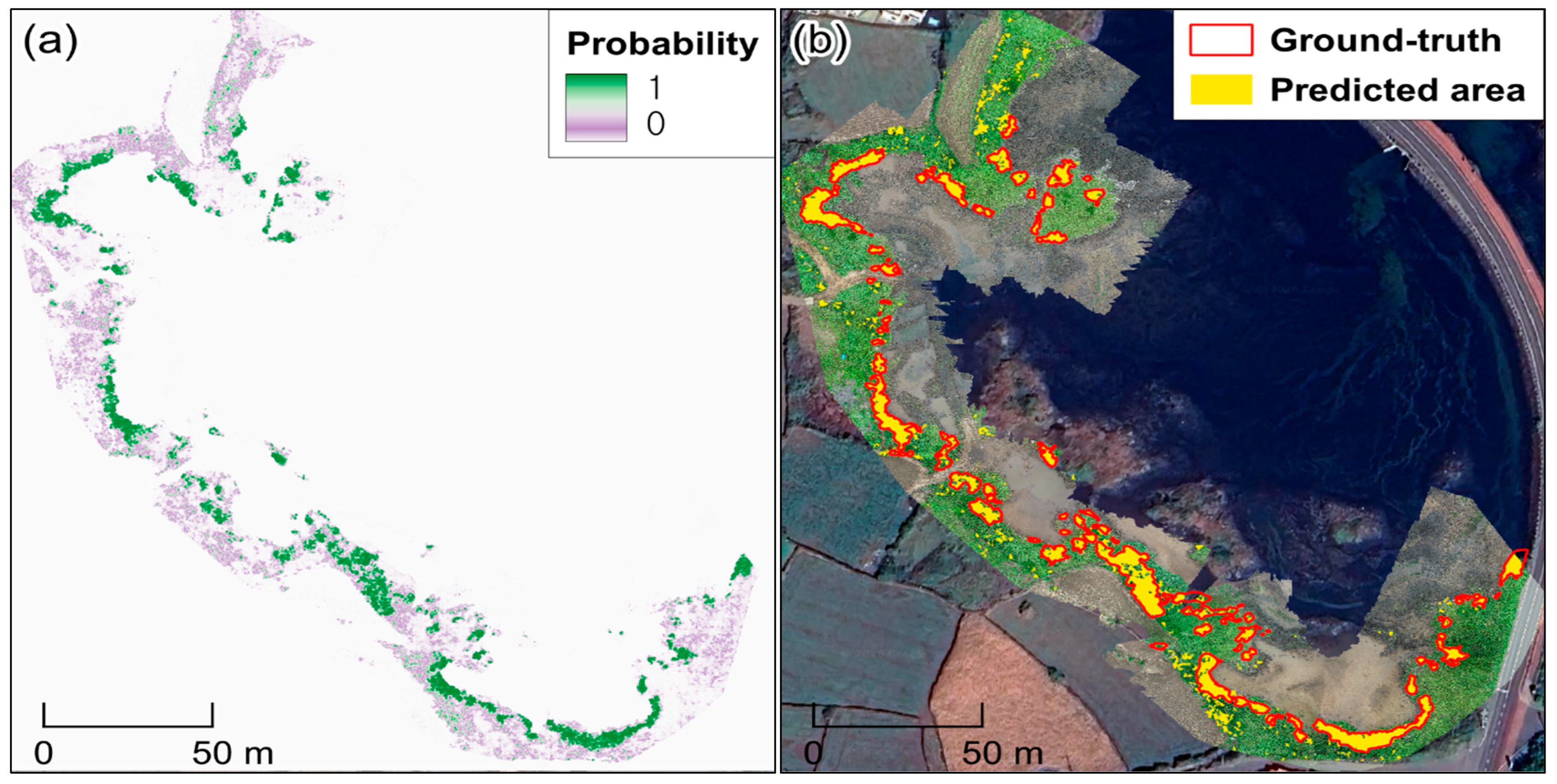
Following the initial optimization with the 1:5 ratio, we conducted a secondary fine-tuning phase using a balanced 1:1 sampling ratio between semi-mangrove and background classes (Figure 5). Quantitatively, the 1:1 fine-tuned model outperformed the initial 1:5 model on the Hado test site, achieving higher semi-mangrove segmentation accuracy (IoU = 0.873) and improved detection quality (precision = 0.943, recall = 0.921), while maintaining a low false-positive rate (FPR = 0.005 vs. 0.007). Consistent with these improvements, the 1:1 fine-tuned output showed sharper, more contiguous patch boundaries and fewer spurious high-probability responses in heterogeneous background areas.
Figure 5.
Effect of 1:1 fine-tuning on predictions at the Hado test site. (a) Semi-mangrove probability map produced after fine-tuning with a balanced 1:1 positive:negative sampling ratio. (b) Binarized prediction (yellow) over the RGB orthomosaic with ground-truth polygons outlined in red.
3.3. Baseline Comparison and Computational Efficiency
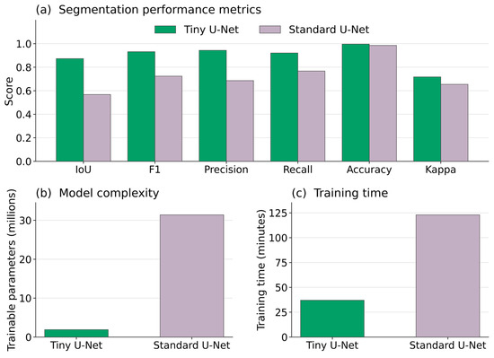
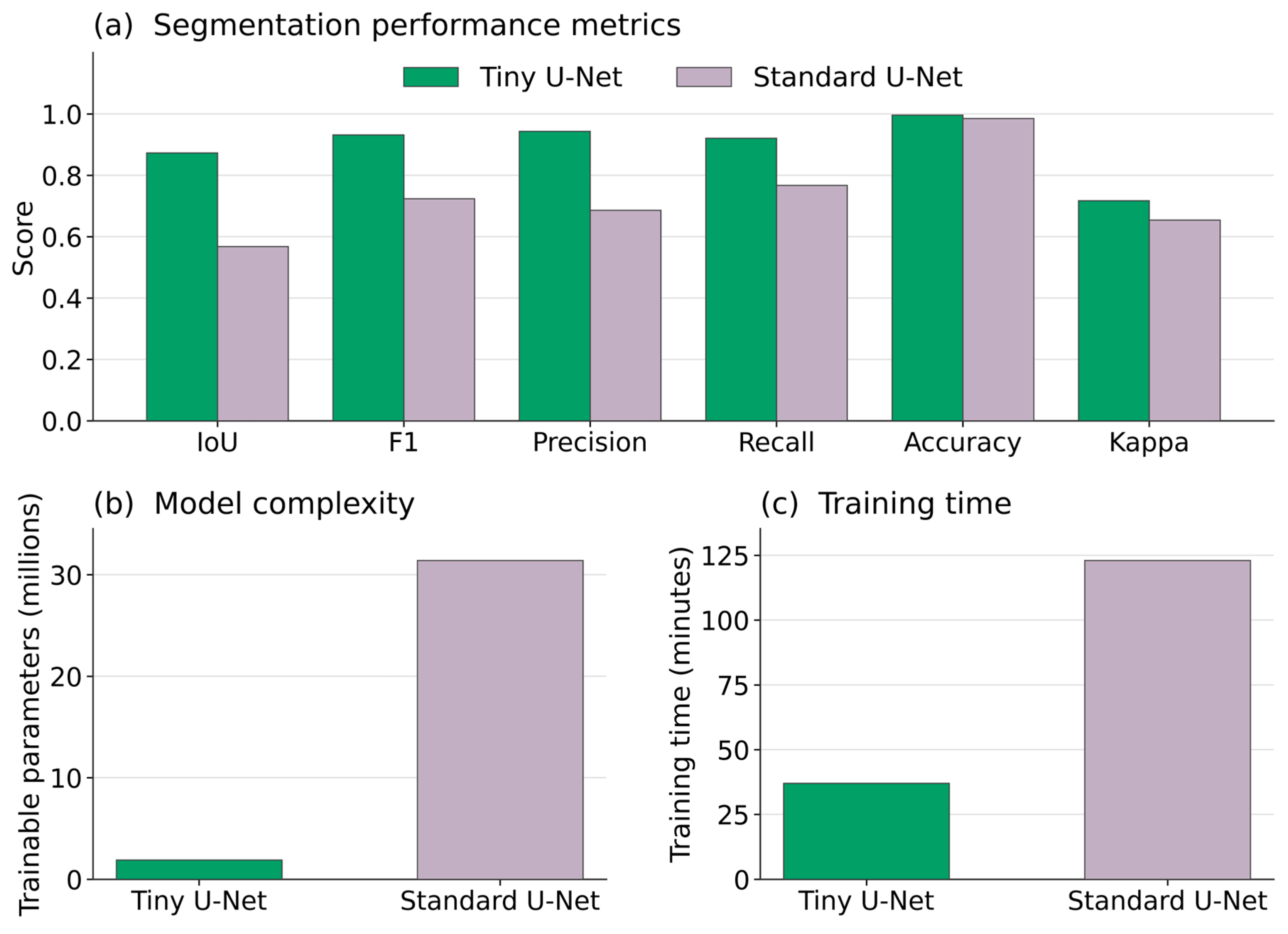
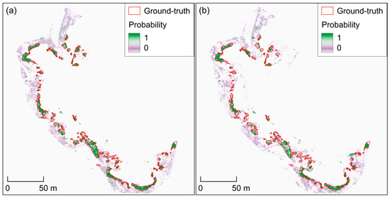
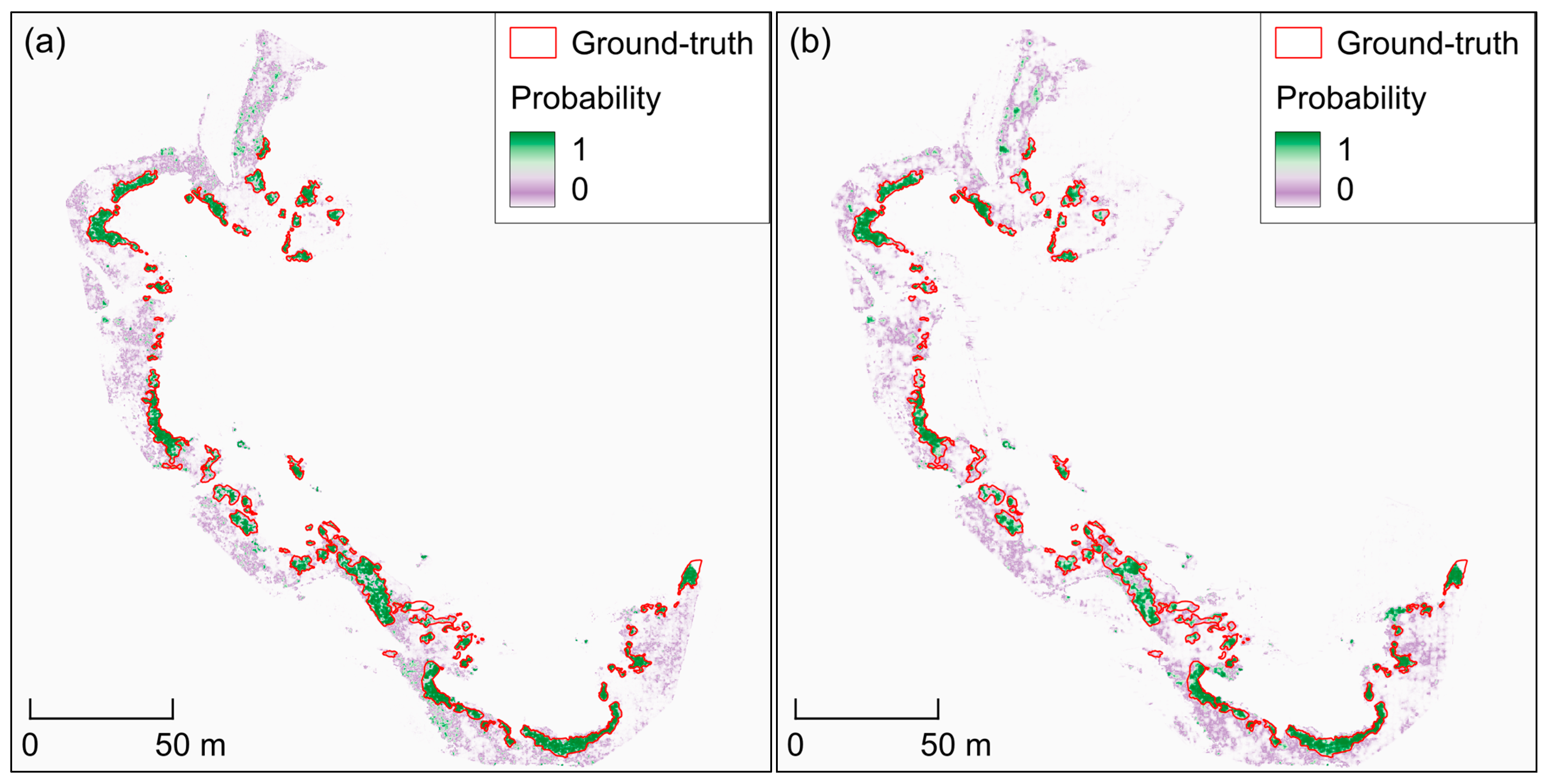
To evaluate the accuracy–efficiency tradeoff of the proposed lightweight architecture, we compared Tiny U-Net with a standard U-Net baseline using the same site-wise split, input tile size, training data, thresholding, post-processing, and evaluation procedure. As shown in Figure 6, the Tiny U-Net outperformed the adopted standard U-Net baseline on the Hado test site across all reported segmentation metrics, including IoU (0.873 vs. 0.568), F1-score (0.932 vs. 0.724), precision (0.943 vs. 0.686), recall (0.921 vs. 0.767), accuracy (0.996 vs. 0.985), and Kappa (0.717 vs. 0.654). In addition, Tiny U-Net required substantially fewer trainable parameters (1.9 M vs. 31.4 M) and shorter training time (37 min vs. 123 min), demonstrating a favorable accuracy–efficiency tradeoff. The probability-map comparison further shows that Tiny U-Net produced more continuous high-confidence responses within the ground-truth polygons and fewer scattered responses in the surrounding background than the standard U-Net (Figure 7).
Figure 6.
Baseline comparison between Tiny U-Net and standard U-Net on the Hado test site. (a) Segmentation performance metrics, including IoU, F1-score, precision, recall, accuracy, and Kappa. (b) Model complexity expressed as the number of trainable parameters. (c) Training time measured under the same hardware and software environment. Tiny U-Net achieved higher segmentation performance while using fewer parameters and requiring less training time than the standard U-Net.
Figure 7.
Probability-map comparison between (a) Tiny U-Net and (b) standard U-Net on the Hado test site. Ground-truth polygons are outlined in red. The purple–green color scale indicates predicted semi-mangrove probability.
3.4. Pooled Pixel-Level Performance Across All Sites
After selecting the final fine-tuned configuration, we evaluated the overall pixel-level performance by pooling predictions across all sites, providing a dataset-wide summary of accuracy and class-specific segmentation quality (Table 3 and Table 4). Because predictions were aggregated over the full dataset, these results reflect overall agreement and error tendencies rather than site-by-site generalization.
Table 3.
Overall pooled pixel-level performance across all sites.
Table 4.
Imbalance-aware statistics aggregated across all sites.
The pooled evaluation yielded an overall accuracy of 0.990 with strong background rejection (specificity = 0.993) (Table 3). For the semi-mangrove class, the model achieved a precision = 0.771 and an F1-score = 0.807. IoU was 0.677 for the semi-mangrove and 0.989 for the background, yielding a mean IoU of 0.833. Overall, these results indicate useful semi-mangrove mapping performance with strong background rejection across the pooled dataset.
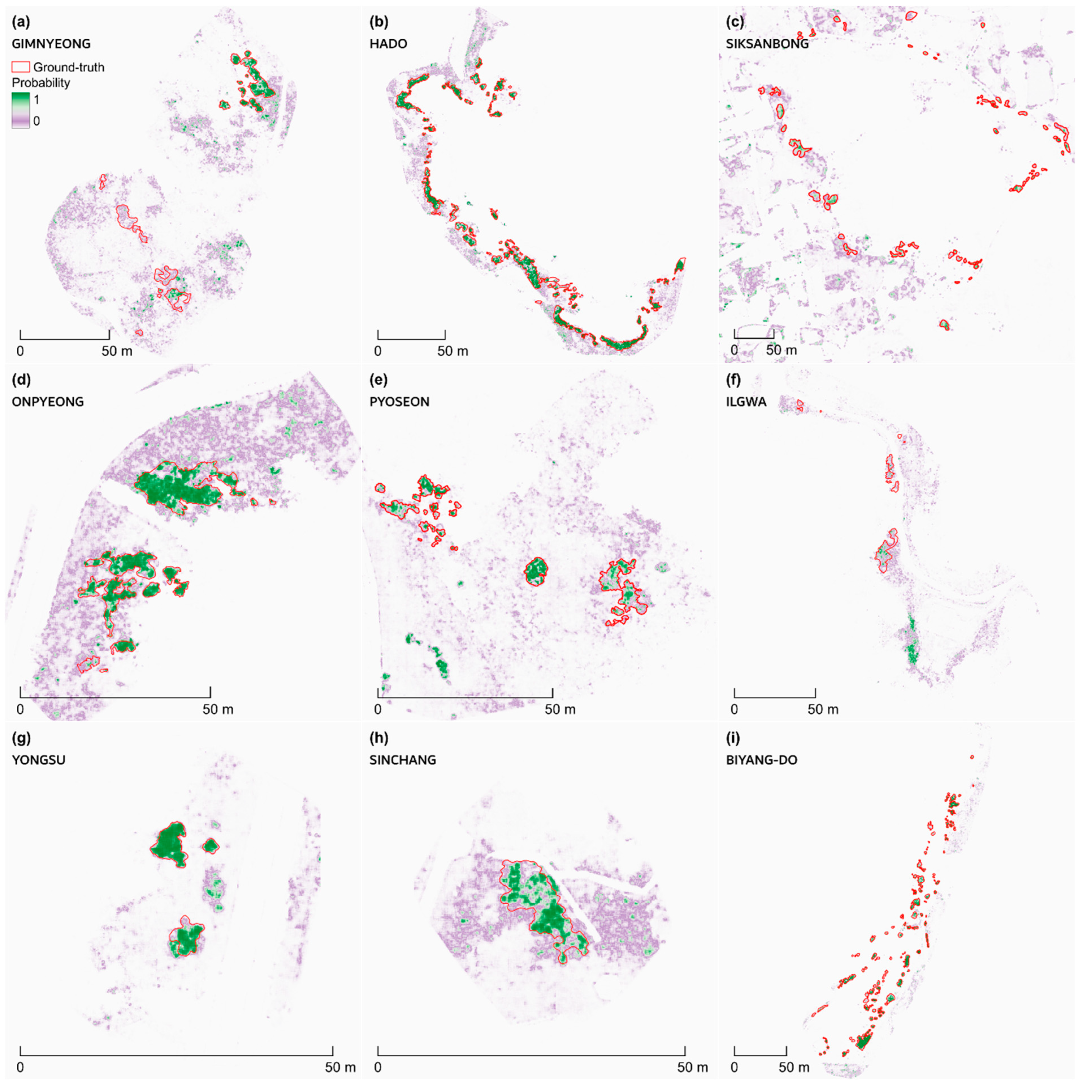
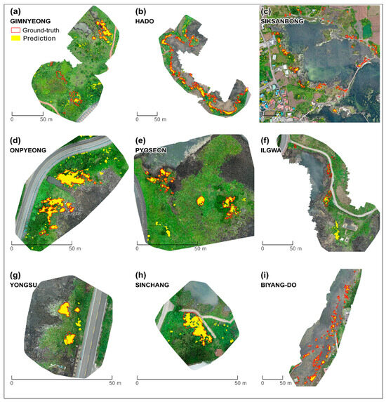
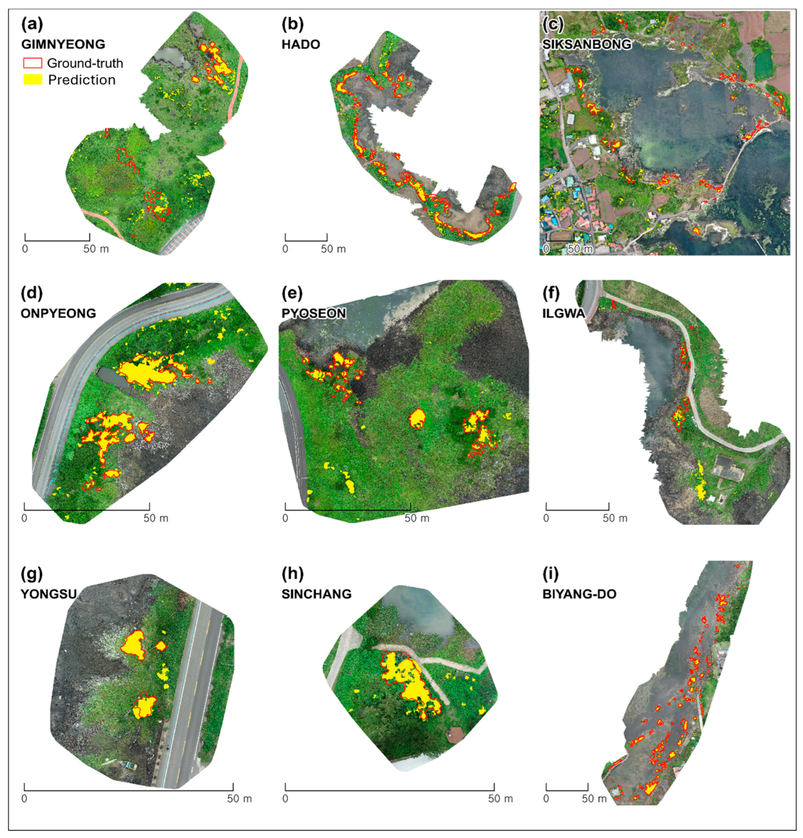
To quantify class imbalance and its impact on errors, we report imbalance-aware metrics derived from pooled confusion counts (Table 4). Across 18,417,277 evaluated pixels, semi-mangrove pixels were rare (prevalence = 2.59%). The pooled confusion counts were 17,819,527 true negatives, 120,370 false positives, 72,674 false negatives, and 404,706 true positives. Among true semi-mangrove pixels, 15.2% were missed (FNR), whereas only 0.7% of background pixels were falsely predicted as semi-mangrove (FPR). The model maintained a high negative predictive value (0.996) despite remaining omissions (FNR = 0.152). Balanced accuracy was 0.921 and Cohen’s Kappa was 0.800. The predicted positive fraction (2.85%) closely matched the true prevalence (2.59%), indicating no substantial overprediction of semi-mangrove extent. To complement the pooled pixel-level metrics, Figure 8 summarizes the final model’s binarized semi-mangrove predictions across all sites, with corresponding probability maps shown in Figure A2 in Appendix B.
Figure 8.
Binary semi-mangrove maps across all sites using the final fine-tuned model. Predicted semi-mangrove extent is shown as a binarized mask overlaid on the orthomosaic for each site (panels (a–i)). Ground-truth polygons are outlined in red, and the binarized model prediction is shown in yellow.
3.5. Qualitative Visualization and Error Interpretation of Model Outputs
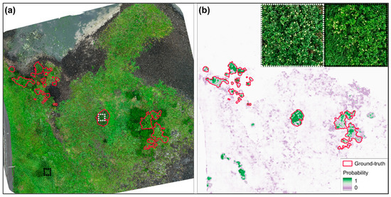
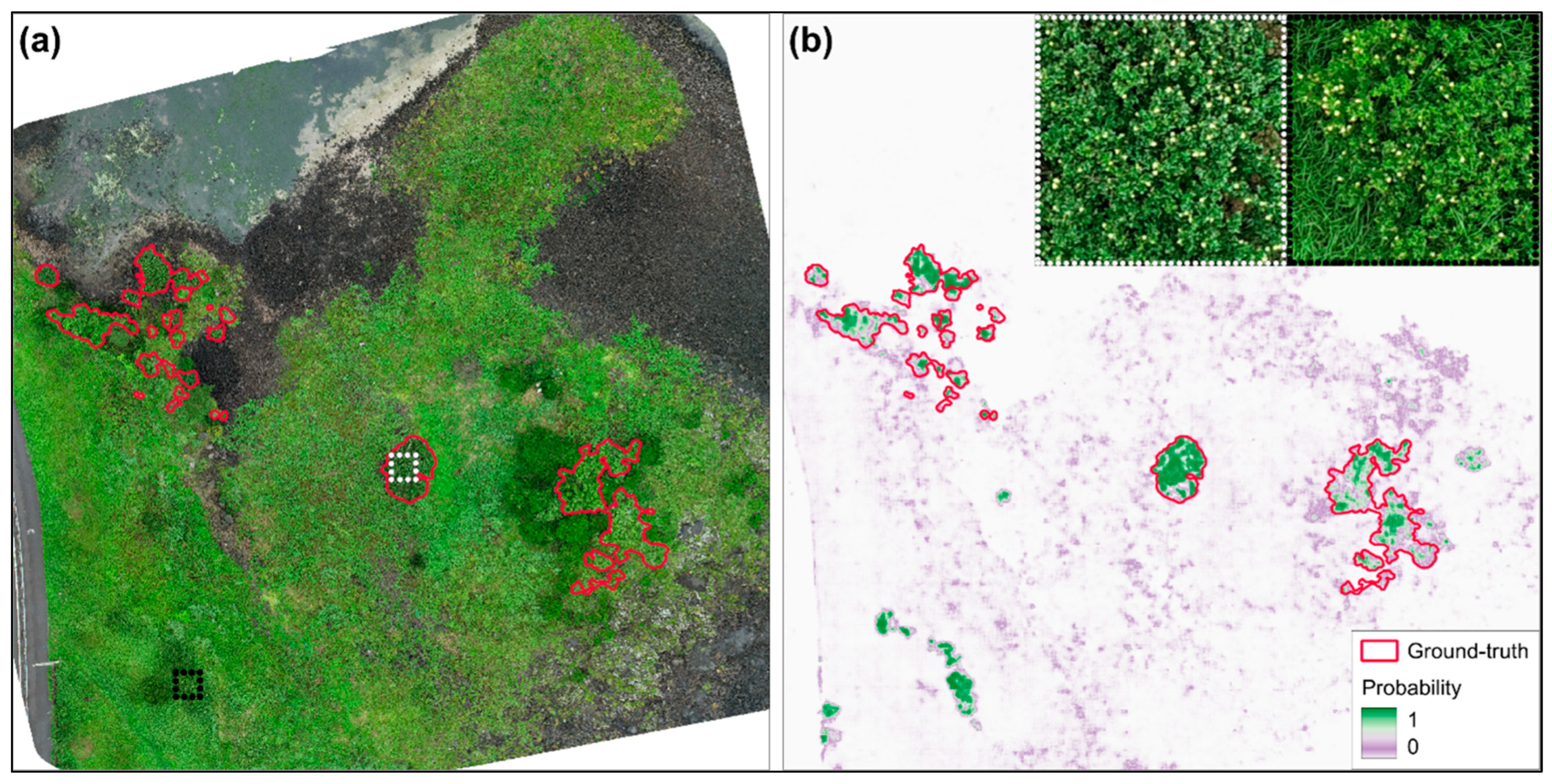
Figure 9 shows the final model’s pixel-wise semi-mangrove probability map for the Pyoseon site (0–1, where higher values indicate greater confidence) and highlights high-confidence responses outside of the ground-truth polygons. While the binary mask provides a definitive segmentation at a selected threshold, the probability map visualizes spatial confidence and supports the identification of candidate patches for follow-up inspection. Insets in panel (b) provide close-up orthomosaic views of H. hamabo: (left) an expert-labeled semi-mangrove patch and (right) a high-confidence candidate area outside of the labeled polygons with similar texture and color patterns. Because separate ground-truth labels were not prepared for error-source classes such as shadows, wet substrate, similar vegetation, or boundary uncertainty, these error patterns were interpreted qualitatively rather than as statistical error-type classes.
Figure 9.
Semi-mangrove probability map and candidate patch examples at the Pyoseon site. (a) RGB orthomosaic with ground-truth polygons outlined in red; white and black dotted boxes indicate an established patch and a high-confidence candidate outside of the labels, respectively. (b) Predicted probability map, where purple = 0, green = 1, with ground-truth polygons outlined in red; insets show close-ups of the boxed regions in (a).
4. Discussion
In this study, we show that Jeju Island semi-mangrove communities (H. hamabo and P. ramosissimus) can be mapped at the centimeter scale from UAV RGB orthomosaics using a lightweight Tiny U-Net semantic segmentation workflow. The results indicate that this approach can extract rare and fragmented semi-mangrove patches while maintaining low false-positive rates under strong class imbalance. The probability maps also provide useful decision-support layers for survey targeting and iterative label refinement, consistent with fine-scale monitoring recommendations [25]. The main contribution of this study is not a completely new segmentation architecture but a practical UAV RGB-based workflow that combines lightweight segmentation, imbalance-aware training, site-wise evaluation, and probability-map interpretation for rare coastal shrub mapping. This type of high-resolution baseline is especially valuable in Jeju’s temperate–subtropical transition zone, where coastal woody vegetation near poleward limits can respond rapidly and nonlinearly to extreme events [12,13]. More broadly, the workflow can be adapted to mapping other rare, patchy coastal shrubs in complex backgrounds, consistent with recent UAV deep learning mangrove studies [41,42].
4.1. Semi-Mangroves at a Poleward Boundary
Jeju Island is a useful boundary setting for tracking coastal woody vegetation because ecological responses near poleward limits can be abrupt and threshold-like. Evidence from poleward mangrove margins shows that mangrove expansion can coincide with salt marsh decline [11,13] and has been linked particularly to decreases in the frequency of extreme cold events [12]. Although the target taxa here are semi-mangroves (mangrove associates) rather than true mangroves, contrasts in leaf traits and salt ion contents between true mangroves and associates indicate different osmotic and ionic strategies and stress tolerances, supporting the need to monitor associates explicitly rather than assuming that they behave like tropical mangrove forests [7]. This distinction matters in Jeju coastal ecotones because shrub patches are small, fragmented, and potentially sensitive to shifts in winter extremes, hydrology, and disturbance regimes, and coarse land-cover products are unlikely to resolve such boundary dynamics. In this context, our centimeter-scale baseline and probability-guided mapping framework provide a practical foundation for detecting patch nucleation, boundary shifts, and disturbance responses. These characteristics also create a challenging mapping problem because the target occurs as sparse, fragmented patches against a dominant and heterogeneous background, which motivates the imbalance-focused interpretation in Section 4.2.
The conservation value of a fine-scale baseline is also practical. Jeju coastal dunes and adjacent coastal habitats are under strong development and tourism pressure, increasing the need for spatially explicit inventories that can support restoration planning and impact assessment [38]. Recent Korean work on H. hamabo communities reports clear geographic and coastal-type structuring and identifies key environmental controls on community distribution [16], but translating this ecological understanding into management requires precise spatial data on where fragmented patches occur and how they change. Jeju-focused semi-mangrove carbon modeling further suggests that these systems can contribute to meaningful aboveground carbon accumulation and that spatial variation is environmentally structured, so improved extent maps can directly reduce uncertainty in carbon-related assessments [3]. Because long-term trend inference is sensitive to methodological choices and uncertainty sources in satellite time-series analysis, establishing a high-quality baseline now also improves the interpretability of future change detection [43]. Accordingly, the site-validated occurrence layers produced here support conservation monitoring and provide a spatial basis for downstream applications such as habitat suitability analysis and carbon-related assessments.
4.2. Mapping Rarity in Complex Backgrounds
Mapping rare, fragmented vegetation is fundamentally different from mapping dominant land-cover types because both training and evaluation can be dominated by the background class. When the target occupies only a small fraction of pixels, overall accuracy can remain high even if the model produces many spurious detections or misses small patches, so the more meaningful question becomes whether the workflow controls false positives while still recovering minority-class structure. This is why imbalance-aware reporting, including balanced accuracy, precision and recall, and IoU or F1, is essential for interpreting performance in rare-class segmentation [35,36]. In practical coastal monitoring, the operational cost of false positives is often higher than small fluctuations in overall accuracy because even a modest false-positive rate can inflate the mapped area and misdirect field surveys when the background vastly outnumbers the target [36].
In this study, semi-mangroves accounted for only 2.59% of pixels, but the final model maintained high balanced accuracy and a low false-positive rate, indicating limited overprediction while still capturing fragmented shrub patches (Table 3 and Table 4). The two-stage sampling strategy helped balance background discrimination and rare-class recovery. The 1:5 initial stage exposed the model to diverse background conditions, including rocks, water margins, shadows, wet substrates, and non-target vegetation, which helped reduce false-positive responses in heterogeneous coastal backgrounds. The later 1:1 fine-tuning stage increased the relative contribution of rare semi-mangrove samples after the model had learned broad background variability, improving target patch extraction.
The composite loss function supported the same objective at the pixel level. Binary cross-entropy (BCE) provided stable pixel-wise optimization, focal loss emphasized hard pixels by down-weighting easy background pixels [24], and Tversky loss helped control the false-positive and false-negative trade-off under class imbalance [34,35]. Together, the sampling strategy and composite loss reduced overprediction while maintaining recall for fragmented semi-mangrove patches. This combination is important for operational monitoring because false positives can inflate the mapped area and misdirect field verification, whereas false negatives may cause small, fragmented patches to be missed. More broadly, this workflow may be adapted to other rare coastal vegetation targets that are sparse and embedded in heterogeneous backgrounds, but broader testing across additional sites and seasons is still needed.
4.3. Probability Maps for Operational Workflows
The probability surfaces produced by the model are not only intermediate outputs but decision-support layers that can be integrated into monitoring and management workflows. Instead of forcing a single hard classification everywhere, probability maps allow users to prioritize review and field verification in places where semi-mangroves occur as small, discontinuous patches embedded in heterogeneous substrates. In our case, the probability output highlighted candidate occurrences outside of the labeled polygons, illustrating how model inference can support iterative inventory refinement while keeping mapping conservative when thresholds are chosen to control false positives (Figure 9). This emphasis on repeatability, validation, and fit-for-purpose products is consistent with guidance for fine-scale mangrove monitoring [25,44] and with recent UAV deep learning studies that use model outputs to support field verification in sparse-target settings [42,45].
Operationally, probability-guided mapping can be implemented as a simple and repeatable cycle. Standardized UAV RGB acquisition supports comparability across time [25,44,46]. Model inference then produces both a binary mask and a probability surface, which can be used to define confidence tiers for review, such as high-confidence areas for polygon confirmation and moderate-confidence edges for targeted inspection. Confirmed new patches could then be added to the training set to improve robustness across sites and acquisition dates, creating a practical label-update loop that is well suited to boundary populations where true distributions are patchy and incomplete.
Probability-guided products also enable management-relevant indicators beyond the total extent. Because monitoring questions often depend on fragmentation, edge dynamics, and canopy discontinuities, future monitoring could use derived polygons and probability surfaces to quantify patch number, edge complexity, and persistence while reducing sensitivity to small threshold shifts. This aligns with UAV studies showing that accounting for canopy gaps can improve area estimation [47] and that segmentation outputs can be translated into interpretable stand-structure indicators for health assessment [41]. For Jeju semi-mangroves, this provides a clear pathway from probability-guided detection to repeatable monitoring of distribution and structural change. It could also be coupled with broader regional screening approaches, where satellite products guide where to deploy UAV surveys [21,48].
4.4. Limitations
This study has several limitations that also suggest clear priorities for future work. First, reliance on UAV RGB orthomosaics is a deliberate operational choice that supports low-cost and repeatable surveys. At the same time, although RGB-only imagery has practical advantages for routine monitoring, it may limit spectral separability, so confusion with visually similar shrubs, wet substrates, and shadows can persist, especially along patch edges. Adding red-edge or NIR bands and structural information such as DSM or LiDAR could improve robustness [29,32]. Second, temporal generalization remains uncertain because all UAV images were acquired in July 2023, and canopy appearance may vary with season, illumination, tidal wetness, and disturbance. Multi-season and multi-year acquisitions with explicit domain-shift testing and standardized protocols would strengthen change detection [25,43,44]. Third, although ground-truth polygons were based on field-confirmed GPS records and expert visual interpretation, label uncertainty may remain along blurred patch edges, and some small individuals or candidate patches may be missed during manual digitization. Probability-guided field verification and iterative label updates can mitigate this, but they require transparent thresholds and validation design [25]. In addition, separate ground-truth labels were not prepared for error-source classes such as shadows, wet substrate, similar vegetation, or boundary uncertainty. Therefore, error-source interpretation in this study was qualitative rather than statistical. Fourth, although the site-wise split reduced spatial leakage, only one validation site and one independent test site were available. Therefore, the results should be interpreted as an initial site-wise transferability assessment within the surveyed Jeju sites rather than as full regional generalization. Finally, mapping H. hamabo and P. ramosissimus as a combined semi-mangrove class limits species-level ecological interpretation. Future species-level discrimination will require more balanced species-specific samples, richer spectral or structural inputs and expanded training data [7,29].
5. Conclusions
This study provides a site-validated, centimeter-scale baseline of Jeju Island semi-mangrove distribution using UAV RGB orthomosaics and a lightweight Tiny U-Net segmentation workflow. The lightweight architecture reduced model size and training time compared with a standard U-Net while maintaining strong semi-mangrove extraction performance. The outputs include binary extent maps and probability surfaces that support conservative delineation, targeted field verification, and iterative inventory refinement. This is important because boundary populations often change through small and discontinuous gains or losses that are difficult to detect with coarse-resolution products. A reliable fine-scale baseline is therefore needed to interpret future expansion, contraction, and fragmentation. More importantly, the workflow can be adapted for other rare and patchy coastal vegetation targets where operational mapping requires both small-patch detection and control of false positives. The combination of two-stage sampling and composite loss functions helped address severe class imbalance by improving rare-class extraction while limiting overprediction in heterogeneous coastal backgrounds. Future work can use this baseline as the first layer of a repeatable Jeju semi-mangrove monitoring system, where newly acquired UAV images can be compared with the present maps to detect patch expansion, contraction, and fragmentation over time. In this way, the workflow can move beyond one-time mapping toward operational ecological monitoring and provide spatial evidence for conservation planning, field survey prioritization, and management of coastal transition zones.
Author Contributions
K.F.: writing—original draft, writing—review and editing, methodology, visualization, formal analysis. J.K.: writing—review and editing, data curation, visualization. B.L.: writing—review and editing, resources, investigation, data curation. M.M.: writing—original draft, writing—review and editing, methodology, visualization, supervision, funding acquisition, conceptualization. All authors have read and agreed to the published version of the manuscript.
Funding
This research was funded by the Warm–Temperate and Subtropical Forest Research Center, National Institute of Forest Science (NIFoS), Republic of Korea (FE0100-2022-04-2025), and supported by the National Research Foundation of Korea (NRF) grant funded by the Korean government (RS-2025-00513070).
Data Availability Statement
The raw data supporting the conclusions of this article will be made available by the authors on request.
Acknowledgments
The authors sincerely thank the editor and the two anonymous reviewers for their constructive comments and suggestions, which helped improve the quality of this manuscript. The authors are pleased to acknowledge that the computational work reported on in this paper was performed on the Shared Computing Cluster which is administered by Boston University’s Research Computing Services.
Conflicts of Interest
The authors declare no competing interests.
Appendix A. Standard U-Net Baseline Configuration and Computing Environment
The standard U-Net baseline was implemented as a reference architecture for evaluating the accuracy–efficiency tradeoff of Tiny U-Net. The model followed the conventional U-Net encoder–decoder design proposed by Ronneberger et al. [31] but was adapted for this study by using 512 × 512 × 3 UAV RGB input tiles and pixel-aligned binary probability-map outputs. The baseline used four encoder stages, one bottleneck, four decoder stages, skip concatenations between corresponding encoder and decoder levels, and a final 1 × 1 convolution followed by sigmoid activation for binary semi-mangrove prediction. This adapted standard U-Net was trained and evaluated under the same data split, tiling, loss function, threshold selection, post-processing, and evaluation protocol as Tiny U-Net. The architecture and computing settings used for the baseline comparison are summarized in Figure A1 and Table A1.
Figure A1.
An adopted standard U-Net baseline architecture used for comparison with Tiny U-Net. The baseline follows the conventional U-Net encoder–decoder structure with four down-sampling stages, a bottleneck, four up-sampling stages, skip connections, and a final 1 × 1 convolution for binary semi-mangrove prediction. Unlike the original U-Net implementation of Ronneberger et al. [31], this baseline was adapted for 512 × 512 UAV RGB input tiles and pixel-aligned 512 × 512 probability-map outputs.
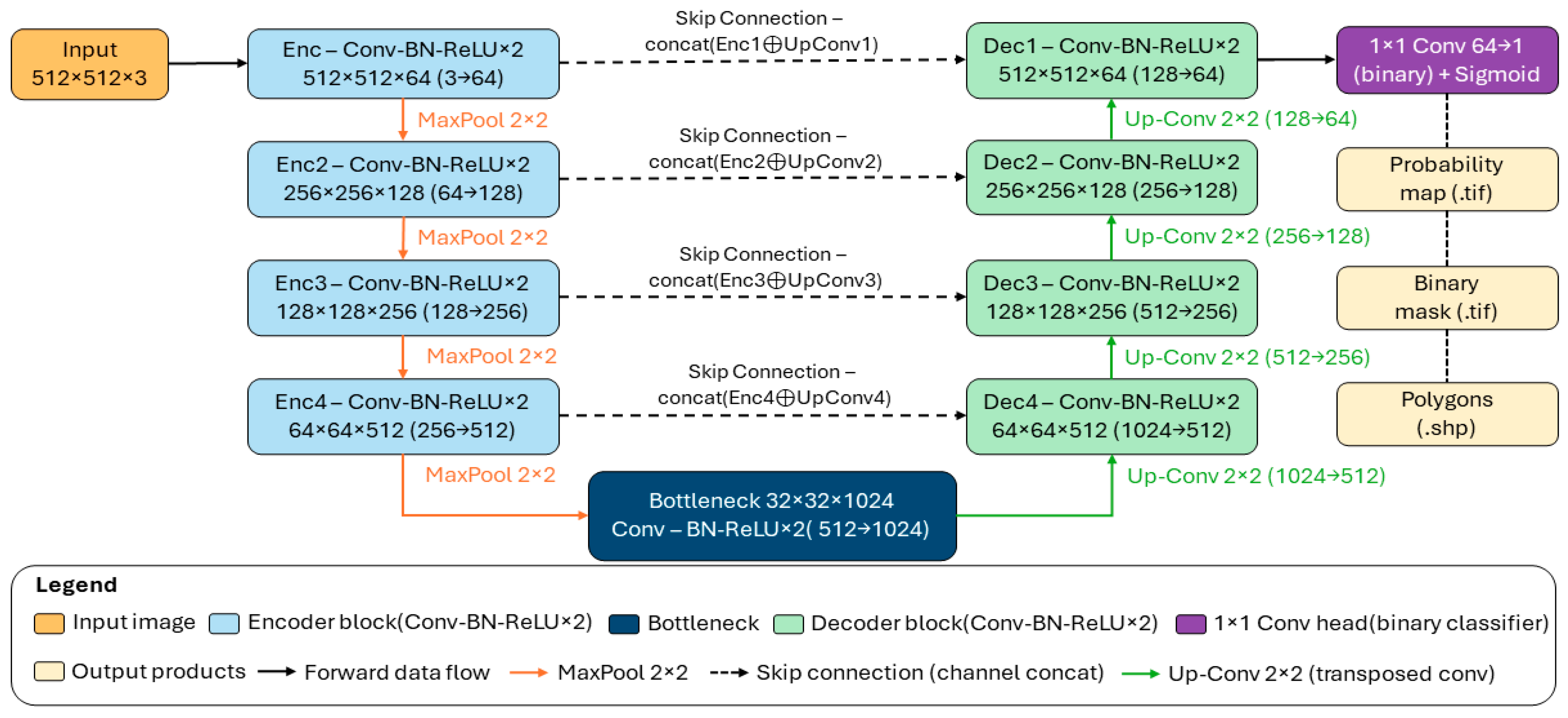
Table A1.
Computing environment used for Tiny U-Net and standard U-Net.
Appendix B
Figure A2.
Semi-mangrove probability maps across all sites using the final fine-tuned model. Predicted probability maps (purple = 0, green = 1) are overlaid on the orthomosaic for each site (panels (a–i)), with ground-truth polygons outlined in red.
References
- Donato, D.C.; Kauffman, J.B.; Murdiyarso, D.; Kurnianto, S.; Stidham, M.; Kanninen, M. Mangroves among the most carbon-rich forests in the tropics. Nat. Geosci. 2011, 4, 293–297. [Google Scholar] [CrossRef] [Scilit]
- Hu, Z.; Temmerman, S.; Zhu, Q.; Wang, X.; Wu, J.; Xu, T.; Schoutens, K.; Suzuki, T.; Yang, Z.; Bouma, T.J. Predicting nature-based coastal protection by mangroves under extreme waves. Proc. Natl. Acad. Sci. USA 2025, 122, e2410883122. [Google Scholar] [CrossRef] [Scilit] [PubMed]
- Lee, C.; Lee, J.; Chaebin, K.; Chu, Y.; Lee, B. Prediction of Carbon Accumulation within Semi-Mangrove Ecosystems Using Remote Sensing and Artificial Intelligence Modeling in Jeju Island. Ecol. Resilient Infrastruct. 2023, 10, 161–170. [Google Scholar] [CrossRef]
- Rogers, A.; Mumby, P.J. Mangroves reduce the vulnerability of coral reef fisheries to habitat degradation. PLoS Biol. 2019, 17, e3000510. [Google Scholar] [CrossRef] [Scilit]
- Wang, M.; Zhang, T.; Xie, Y.; Zhang, Z.; Wu, X. Mapping accumulated carbon storage of global mangroves from 2000 to 2020 at a 1 km resolution. Sci. Data 2025, 12, 552. [Google Scholar] [CrossRef] [Scilit]
- Coldren, G.A.; Langley, J.A.; Feller, I.C.; Chapman, S.K.; Silliman, B. Warming accelerates mangrove expansion and surface elevation gain in a subtropical wetland. J. Ecol. 2019, 107, 79–90. [Google Scholar] [CrossRef] [Scilit]
- Wang, L.; Mu, M.; Li, X.; Lin, P.; Wang, W. Differentiation between true mangroves and mangrove associates based on leaf traits and salt contents. J. Plant Ecol. 2011, 4, 292–301. [Google Scholar] [CrossRef] [Scilit]
- Osland, M.J.; Hughes, A.R.; Armitage, A.R.; Scyphers, S.B.; Cebrian, J.; Swinea, S.H.; Shepard, C.C.; Allen, M.S.; Feher, L.C.; Nelson, J.A.; et al. The impacts of mangrove range expansion on wetland ecosystem services in the southeastern United States: Current understanding, knowledge gaps, and emerging research needs. Glob. Change Biol. 2022, 28, 3163–3187. [Google Scholar] [CrossRef] [Scilit]
- Ribas-Deulofeu, L.; Loubeyres, M.; Denis, V. Jeju Island a sentinel for tracking ocean warming impacts on high-latitude benthic communities. Coral Reefs 2023, 42, 1097–1112. [Google Scholar] [CrossRef] [Scilit]
- Campbell, A.D.; Fatoyinbo, L.; Goldberg, L.; Lagomasino, D. Global hotspots of salt marsh change and carbon emissions. Nature 2022, 612, 701–706. [Google Scholar] [CrossRef] [Scilit]
- Cavanaugh, K.C.; Dangremond, E.M.; Doughty, C.L.; Williams, A.P.; Parker, J.D.; Hayes, M.A.; Rodriguez, W.; Feller, I.C. Climate-driven regime shifts in a mangrove-salt marsh ecotone over the past 250 years. Proc. Natl. Acad. Sci. USA 2019, 116, 21602–21608. [Google Scholar] [CrossRef] [Scilit] [PubMed]
- Cavanaugh, K.C.; Kellner, J.R.; Forde, A.J.; Gruner, D.S.; Parker, J.D.; Rodriguez, W.; Feller, I.C. Poleward expansion of mangroves is a threshold response to decreased frequency of extreme cold events. Proc. Natl. Acad. Sci. USA 2014, 111, 723–727. [Google Scholar] [CrossRef] [Scilit]
- Saintilan, N.; Wilson, N.C.; Rogers, K.; Rajkaran, A.; Krauss, K.W. Mangrove expansion and salt marsh decline at mangrove poleward limits. Glob. Change Biol. 2014, 20, 147–157. [Google Scholar] [CrossRef] [Scilit]
- Plants of the World Online. Hibiscus hamabo Siebold & Zucc. Available online: https://powo.science.kew.org/taxon/urn:lsid:ipni.org:names:560323-1 (accessed on 29 April 2026).
- Plants of the World Online. Paliurus ramosissimus (Lour.) Poir. Available online: https://powo.science.kew.org/taxon/urn:lsid:ipni.org:names:717703-1 (accessed on 29 April 2026).
- Park, E.-H.; Lee, B.-R.; Yang, J.-E.; Park, M.-J.; Choi, B.-K. Distribution and Vegetation Characteristics of Semi-mangrove Hibisus hamabo in Korea. Korean J. Environ. Ecol. 2024, 38, 354–366. [Google Scholar] [CrossRef] [Scilit]
- Wang, L.; Jia, M.M.; Yin, D.M.; Tian, J.Y. A review of remote sensing for mangrove forests: 1956-2018. Remote Sens. Environ. 2019, 231, 111223. [Google Scholar] [CrossRef] [Scilit]
- Wei, S.; Zhang, H.S.; Ling, J. A review of mangrove degradation assessment using remote sensing: Advances, challenges, and opportunities. GISci. Remote Sens. 2025, 62, 2491920. [Google Scholar] [CrossRef] [Scilit]
- Lu, Y.; Wang, L. How to automate timely large-scale mangrove mapping with remote sensing. Remote Sens. Environ. 2021, 264, 112584. [Google Scholar] [CrossRef] [Scilit]
- Xu, C.; Wang, J.L.; Sang, Y.; Li, K.; Liu, J.X.; Yang, G. An Effective Deep Learning Model for Monitoring Mangroves: A Case Study of the Indus Delta. Remote Sens. 2023, 15, 2220. [Google Scholar] [CrossRef] [Scilit]
- Tran, T.V.; Reef, R.; Zhu, X.; Gunn, A. Characterising the distribution of mangroves along the southern coast of Vietnam using multi-spectral indices and a deep learning model. Sci. Total Environ. 2024, 923, 171367. [Google Scholar] [CrossRef] [Scilit]
- Xia, Q.; Qin, C.Z.; Li, H.; Huang, C.; Su, F.Z. Mapping Mangrove Forests Based on Multi-Tidal High-Resolution Satellite Imagery. Remote Sens. 2018, 10, 1343. [Google Scholar] [CrossRef] [Scilit]
- Reyes, G.J.; Smyth, A.R.; Qiu, J.; Reynolds, L.K. Highly Urbanized Mangrove Areas are Small in Size, Fragmented, and Missed by Large-scale Mapping Efforts. Wetlands 2024, 44, 103. [Google Scholar] [CrossRef] [Scilit]
- Lin, T.Y.; Goyal, P.; Girshick, R.; He, K.M.; Dollár, P. Focal Loss for Dense Object Detection. In 2017 IEEE International Conference on Computer Vision (ICCV); IEEE: New York, NY, USA, 2017; pp. 2999–3007. [Google Scholar] [CrossRef] [Scilit]
- Schill, S.R.; McNulty, V.P.; Perez, D.; Shono, K.; Friedman, K. Remote Sensing Techniques for Mapping and Monitoring Mangroves at Fine Scales; FAO: Rome, Italy, 2024; p. 94. [Google Scholar]
- Zhang, H.; Wei, S.; Liang, X.; Chen, Y.; Zhang, H. Scale effects in mangrove mapping from ultra-high-resolution remote sensing imagery. Int. J. Appl. Earth Obs. Geoinf. 2025, 136, 104310. [Google Scholar] [CrossRef] [Scilit]
- Hsu, A.J.; Kumagai, J.; Favoretto, F.; Dorian, J.; Guerrero Martinez, B.; Aburto-Oropeza, O. Driven by Drones: Improving Mangrove Extent Maps Using High-Resolution Remote Sensing. Remote Sens. 2020, 12, 3986. [Google Scholar] [CrossRef] [Scilit]
- Cao, J.J.; Leng, W.C.; Liu, K.; Liu, L.; He, Z.; Zhu, Y.H. Object-Based Mangrove Species Classification Using Unmanned Aerial Vehicle Hyperspectral Images and Digital Surface Models. Remote Sens. 2018, 10, 89. [Google Scholar] [CrossRef] [Scilit]
- Chen, X.; Zhang, X.; Zhuang, C.; Dai, X.; Kong, L.; Xie, Z.; Hu, X. An Approach for Detecting Mangrove Areas and Mapping Species Using Multispectral Drone Imagery and Deep Learning. Sensors 2025, 25, 2540. [Google Scholar] [CrossRef] [Scilit]
- Yang, Y.Z.; Meng, Z.J.; Zu, J.X.; Cai, W.H.; Wang, J.L.; Su, H.X.; Yang, J. Fine-Scale Mangrove Species Classification Based on UAV Multispectral and Hyperspectral Remote Sensing Using Machine Learning. Remote Sens. 2024, 16, 3093. [Google Scholar] [CrossRef] [Scilit]
- Ronneberger, O.; Fischer, P.; Brox, T. U-Net: Convolutional Networks for Biomedical Image Segmentation. In Medical Image Computing and Computer-Assisted Intervention–MICCAI 2015; Lecture Notes in Computer Science; Springer: Cham, Switzerland, 2015; pp. 234–241. [Google Scholar]
- Fu, L.X.; Wang, Y.R.; Wu, S.L.; Zhuang, J.S.; Wu, Z.Q.; Wu, J.; Chen, H.D.; Chen, Y.K. TCCFNet: A semantic segmentation method for mangrove remote sensing images based on two-channel cross-fusion networks. Front. Mar. Sci. 2025, 12, 1535917. [Google Scholar] [CrossRef] [Scilit]
- Wang, X.; Zhang, Y.; Ca, J.; Qin, Q.; Feng, Y.; Yan, J. Semantic segmentation network for mangrove tree species based on UAV remote sensing images. Sci. Rep. 2024, 14, 29860. [Google Scholar] [CrossRef] [Scilit] [PubMed]
- Salehi, S.S.M.; Erdogmus, D.; Gholipour, A. Tversky loss function for image segmentation using 3D fully convolutional deep networks. In Proceedings of the International Workshop on Machine Learning in Medical Imaging (MLMI); Springer: Cham, Switzerland, 2017; pp. 379–387. [Google Scholar]
- Jadon, S. A survey of loss functions for semantic segmentation. In Proceedings of the 2020 IEEE Conference on Computational Intelligence in Bioinformatics and Computational Biology (CIBCB), Via del Mar, Chile, 27–29 October 2020; IEEE: New York, NY, USA, 2020; pp. 1–7. [Google Scholar]
- Zhou, Z.; Zheng, C.; Liu, X.; Tian, Y.; Chen, X.; Chen, X.; Dong, Z. A Dynamic Effective Class Balanced Approach for Remote Sensing Imagery Semantic Segmentation of Imbalanced Data. Remote Sens. 2023, 15, 1768. [Google Scholar] [CrossRef] [Scilit]
- Perrois, G.; Jöst, A.B.; Lee, K.-T.; Pons, L.M.T.; Yang, H.-S.; Son, Y.B.; Park, H.-S.; Kang, D.-H.; Kim, T. Environmental impact on marginal coastal benthic communities within the Jeju Island, South Korea temperate transition zone. Front. Mar. Sci. 2024, 11, 1345518. [Google Scholar] [CrossRef] [Scilit]
- Kim, K.D. The distribution of Jeju coastal sand dune plants and its restoration implications. Korean Soc. Environ. Restor. Technol. 2024, 27, 31–44. [Google Scholar] [CrossRef]
- Wei, Y.D.; Cheng, Y.C.; Yin, X.B.; Xu, Q.; Ke, J.C.; Li, X.D. Deep Learning-Based Classification of High-Resolution Satellite Images for Mangrove Mapping. Appl. Sci. 2023, 13, 8526. [Google Scholar] [CrossRef] [Scilit]
- Dong, H.; Gao, Y.F.; Chen, R.Q.; Wei, L.F. MangroveSeg: Deep-Supervision-Guided Feature Aggregation Network for Mangrove Detection and Segmentation in Satellite Images. Forests 2024, 15, 127. [Google Scholar] [CrossRef] [Scilit]
- Zhai, C.Y.; Zhang, Y.T.; Wu, Y.F.; Shen, X.X. Accurate Evaluation of Urban Mangrove Forest Health Considering Stand Structure Indicators Based on UAVs. Forests 2025, 16, 1168. [Google Scholar] [CrossRef] [Scilit]
- Zhang, Z.; Shen, X.X.; Yan, C.H.; Li, R.L.; Li, B. Unveiling seaward expansion pattern in mangrove forests using UAV remote sensing and deep learning. Ecol. Indic. 2025, 178, 114054. [Google Scholar] [CrossRef] [Scilit]
- Darabi, H.; Haghighi, A.T.; Klöve, B.; Luoto, M. Remote sensing of vegetation trends: A review of methodological choices and sources of uncertainty. Remote Sens. Appl.-Soc. Environ. 2025, 37, 101500. [Google Scholar] [CrossRef] [Scilit]
- Ngo, D.T.; Nguyen, H.H.V.; Nguyen, B.T.T.; Dang, N.T. Protocol for establishing a map of mangrove species distribution using multispectral unmanned aerial vehicle data. STAR Protoc. 2024, 5, 103425. [Google Scholar] [CrossRef] [Scilit]
- Shendryk, Y.; Vilas, M.P. Detecting mangrove seedlings from UAV imagery using deep learning for restoration monitoring. Sci. Rep. 2026, 16, 719. [Google Scholar] [CrossRef] [Scilit] [PubMed]
- Abu Bakar, N.A.; Wan Mohd Jaafar, W.S.; Abdul Maulud, K.N.; Muhmad Kamarulzaman, A.M.; Saad, S.N.M.; Mohan, M. Monitoring mangrove-based blue carbon ecosystems using UAVs: A review. Geocarto Int. 2024, 39, 2405123. [Google Scholar] [CrossRef] [Scilit]
- Muqorrabin, M.A.; Alwi, R.; Nurdin, N. Enhancing the Precision of Mangrove Area Estimation by Incorporating Canopy Gaps in UAV Methodologies. Int. Arch. Photogramm. Remote Sens. Spat. Inf. Sci. 2025, XLVIII-G-2025, 1095–1102. [Google Scholar] [CrossRef] [Scilit]
- Pinkeaw, S.; Boonrat, P.; Koedsin, W.; Huete, A. Semi-automated mangrove mapping at National-Scale using Sentinel-2, Sentinel-1, and SRTM data with Google Earth Engine: A case study in Thailand. Egypt. J. Remote Sens. Space Sci. 2024, 27, 555–564. [Google Scholar] [CrossRef] [Scilit]

Disclaimer/Publisher’s Note: The statements, opinions and data contained in all publications are solely those of the individual author(s) and contributor(s) and not of MDPI and/or the editor(s). MDPI and/or the editor(s) disclaim responsibility for any injury to people or property resulting from any ideas, methods, instructions or products referred to in the content. |
© 2026 by the authors. Licensee MDPI, Basel, Switzerland. This article is an open access article distributed under the terms and conditions of the Creative Commons Attribution (CC BY) license.