Reliable Underwater Acoustic Telemetry for Ocean Remote Sensing Platforms: Channel-Prediction-Based Adaptive Polar–Raptor Coded OFDM

Highlights

What are the main findings?

• We proposed a two-layer coded OFDM transmission scheme that combines Polar codes for bit-error correction and Raptor codes for packet-erasure recovery.
• The proposed adaptive link achieves a throughput gain of 20–39% compared to fixed-overhead methods across various underwater scenarios, including deep-water environments.

What are the implications of the main findings?

• The study demonstrates that optimal transmission parameters can be determined in real-time through channel prediction (TMSBL and SRUKF), effectively overcoming long propagation delays in underwater links.
• These results provide a robust foundation for enhancing the operational efficiency of underwater platforms, such as AUVs and seabed observatories, by ensuring reliable high-speed data telemetry.

Abstract

Long propagation delays, severe multipaths, and narrow bandwidths make feedback-based link adaptation impractical in UWA channels at kilometer ranges, so we replace the feedback step with a prediction step. The transmitter runs a two-layer coded OFDM link in which Polar codes handle bit errors, and Raptor fountain codes handle packet erasures, with the Raptor overhead (OH) as the only real-time knob. The OH is picked from a lookup table indexed by three quantities the receiver can estimate online: SNR, RMS delay spread, and Doppler frequency. Two CSI predictors feed that table: Temporal Multiple Sparse Bayesian Learning (TMSBL), which exploits delay-domain sparsity, and the Square-Root Unscented Kalman Filter (SRUKF), which tracks per-subcarrier variations. We evaluate the system in five channel environments (AWGN, Rayleigh, K-distribution, Bellhop ray-tracing, and synthetic proxies parameterized from the KAM11 and WATERMARK sea-trial statistics). Across the nine Bellhop scenarios, the adaptive link’s throughput gain over a fixed-OH ($\mathrm{OH}=1.5$) baseline at SNR $=4$ dB spans roughly $-4\%$ to $+30\%$, with the largest benefit in the marginal short-range cases (shallow 500 m, $+30\%$) where the fixed baseline is most over-provisioned and near-parity elsewhere. The scheme’s principal benefit is collapse prevention, tracking the Oracle within the safety margin and avoiding the throughput collapse the fixed baseline suffers at low SNRs. This effect is specific to the physically structured Bellhop channels; in the homogeneous Rayleigh and K-distribution channels, both schemes enter deep outage at very low SNRs, so it is not a universal guarantee. A 1000-trial high-resolution Rayleigh campaign sharpens the head-to-head between predictors: at SNR $=4$ dB, SRUKF + OH reaches PER $0.048$ (95% Wilson CI $[0.036, 0.063]$) and TMSBL + OH reaches $0.071$ ($[0.057, 0.089]$), and at SNR $=12$ dB, their throughputs ($0.748$ and $0.746$) are statistically indistinguishable from each other (95% Wilson halfwidth $\sim \pm$0.014) and lie close to the Oracle’s $0.768$ (within $\sim 0.02$). The two predictors therefore occupy overlapping operating regions once the safety margin is matched, and a sparsity-dependent tendency (TMSBL in sparse multipath, SRUKF in dense multipath) appears only in physically structured channels and only at the $n=100$ screening level, where it is not statistically resolved and would benefit from higher-trial confirmation. A finite-blocklength check confirms that CA-SCL-decoded Polar codes at $N=128$ stay within $0.5$ dB of the Polyanskiy normal approximation, which makes Polar a sensible inner code at UWA block lengths.

1. Introduction

Underwater acoustic (UWA) communication is a key enabling technology for oceanographic observation, underwater vehicle control, and subsea sensor networks [1,2]. The growing demand for real-time ocean monitoring, driven by climate science, offshore operations, and maritime security, has placed stringent requirements on UWA link reliability and throughput. Yet the UWA channel is fundamentally harsher than terrestrial radio channels: sound propagates at only about 1500 m/s (five orders of magnitude slower than electromagnetic waves), so interactive protocols are impractical over long ranges; reflections from the sea surface, seabed, and thermocline produce intense multipaths with delay spreads of tens of milliseconds; relative motion and ocean currents introduce a Doppler spread that renders the channel strongly time-varying; and the usable bandwidth is limited to a few kilohertz [3]. Frequency-dependent absorption further restricts the range: at the 12 kHz carrier frequency used in this work, Thorp’s formula [4] yields an absorption coefficient of approximately 1.2 dB/km, meaning that at a 3 km link the total transmission loss exceeds 60 dB.

Reliable transmission in such environments demands both strong forward error correction (FEC) and adaptive behavior at the link layer. Our response is a Polar–Raptor two-layer coded OFDM system in which only one parameter, the Raptor overhead (OH), is adapted in real time. Overhead sets how much redundancy the transmitter sends. Pick it conservatively, and throughput bleeds away in good channels; pick it aggressively, and there is no margin left when the channel dips. A predictor that can tell those two cases apart makes that choice cheap. Polar codes sit at the physical layer because they dominate the short-blocklength regime, Raptor codes sit on top because they recover erasures without retransmission, and a lookup table (LUT) driven by CSI predictions links them.

1.1. Rationale for Technology Selection

Necessity of Raptor Codes. Automatic repeat request (ARQ) is impractical for UWA links because the slow speed of sound yields round-trip times on the order of a second at kilometer ranges, and half-duplex acoustic modems further increase the latency. Rateless codes, which provide adaptive redundancy in a single transmission, are therefore essential. Raptor codes [5] are fountain codes that generate an essentially unlimited stream of encoded symbols from k source symbols, allowing the receiver to decode upon receiving $k(1+ϵ)$ symbols, where $ϵ$ is the reception overhead (OH). Ke et al. [6] demonstrated joint equalization and Raptor decoding for UWAs, but without adaptive OH selection. Dynamically adjusting the OH in response to predicted channel conditions is the central theme of this work.

Suitability of Polar Codes. Polar codes [7] are the only provably capacity-achieving codes that also perform strongly in the finite-blocklength regime. UWA’s limited bandwidth and short frames mandate block lengths of $N=128$–512, where low-density parity-check (LDPC) and Turbo codes degrade significantly [8]. In contrast, Polar codes with CRC-aided successive cancellation list (CA-SCL) decoding maintain excellent performance across these short blocks; our finite-blocklength check (Section 2.3) stays within $0.5$ dB of the Polyanskiy bound at $N=128$ and within about 2 dB at $N=256$, and this work operates the inner code at $N=256$. This work therefore adopts a two-layer architecture in which Polar codes serve as the physical-layer (PHY) code and Raptor codes provide upper-layer redundancy control, correcting errors at the PHY layer on a per-packet basis and recovering packet losses at the Raptor layer.

1.2. Related Work

The proposed system integrates advances from four research threads, namely, UWA-OFDM design, adaptive coding, channel prediction, and modern coding theory. These threads have matured independently but have not yet been unified for the UWA scenario.

Orthogonal frequency-division multiplexing (OFDM) is the dominant modulation for UWA links, owing to its robustness against frequency-selective fading and its efficient use of the limited acoustic bandwidth [9]. Li et al. [10] demonstrated MIMO-OFDM exceeding 100 kbps in shallow water, and Zhou and Wang [11] provided a comprehensive treatment of synchronization, channel estimation, and equalization. However, such systems invariably employ LDPC or convolutional codes as the FEC component. Only recently have Zhai et al. [12] and Falk et al. [13] investigated Polar codes for UWA, but without Raptor-layer adaptation or CSI prediction. The most recent UWA-OFDM literature (2024–2025) concentrates on the receiver side: Adil et al. [14] and Karim et al. [15] trained transfer-learning and convolution-recurrent networks to demodulate and estimate the channel more accurately, while the AUV-telemetry community treats the physical link as a fixed pipe and optimizes navigation and data scheduling on top of it [16]. These works improve how a frame is received but leave the transmitter-side coding configuration static; none adapts the FEC structure itself to the channel, which is the lever exploited here.

Adaptive transmission itself is a mature area. Goldsmith and Chua [17] laid the theoretical groundwork for adaptive coded modulation (ACM) over fading channels; in the UWA domain, Radosevic et al. [18] validated adaptive OFDM modulation experimentally, and more recent work has added data-driven AMC [19,20]. All of these schemes, however, lean on receiver-to-transmitter feedback, which is precisely the channel UWA propagation delays cripple. Even the latest energy-aware adaptation frameworks follow this template: Ur Rehman et al. [21] used reinforcement learning to tune transmission parameters reactively from the observed network state, and Saha et al. [22] made the Polar codeword length itself adaptive but assumed that the operating point is supplied externally rather than predicted. Our link replaces the feedback step with a prediction step: the transmitter picks its coding parameters from a predicted channel rather than a reported one, and it does so through an offline-built LUT rather than an online learner that must converge in situ.

Accurate channel prediction is the cornerstone of proactive adaptation. Qarabaqi and Stojanovic [23] studied Kalman-filter-based prediction together with statistical channel models that capture the non-Gaussian, non-stationary nature of UWA links. Berger et al. [24] exploited a sparse delay–Doppler structure via compressed sensing, achieving improved estimation with reduced pilot overhead. Machine learning has also been applied: Jiang et al. [25] demonstrated DNN-based channel estimation for UWA-OFDM, and recent work has explored LSTM- and attention-based temporal prediction. Saravanan and Sukumaran [26] pushed this further by feeding deep-learning channel-state forecasts into a stochastic network calculus model for proactive resource control, confirming that prediction-driven adaptation is gaining traction; the predictor, however, is decoupled from the FEC layer and validated only against queueing metrics rather than coded link performance. These methods typically require large training datasets and may lack interpretability in safety-critical deployments. In contrast, the sparse Bayesian learning approach adopted here [27,28,29,30] provides a principled probabilistic framework that naturally captures UWA channel sparsity while offering uncertainty quantification for adaptation decisions.

Fountain codes have attracted attention for UWAs precisely because they eliminate feedback-based retransmission. Luby Transform (LT) codes [31] were the first practical realization but exhibit a non-zero error floor; classical Raptor codes [5] remove this limitation by concatenating an outer pre-code with an inner LT code, achieving linear-time encoding and decoding. Several studies have applied Raptor codes to underwater networks for reliable data dissemination, yet dynamic adjustment of the Raptor overhead based on predicted channel conditions has not been addressed.

Polar codes have moved quickly since Arıkan’s original construction [7]. The CA-SCL decoder of Niu and Chen [32] closed most of the finite-length gap to LDPC and Turbo codes, and at the block lengths UWAs actually use ($N=128$ to 512), the resulting performance approaches the finite-blocklength bounds of Polyanskiy et al. [33]. LDPC and Turbo codes do not match this behavior at these block lengths.

Three gaps therefore remain open in the literature. UWA-OFDM systems continue to rely on conventional FEC codes that underperform at the block lengths UWA frames actually carry, while Polar codes (which are theoretically suited to this regime) have barely been applied to UWAs. Adaptive transmission work for UWAs either assumes perfect CSI or relies on feedback-based schemes that are impractical over long-range acoustic links, leaving predictive adaptation largely unexplored. And while sparse Bayesian and Kalman-based channel predictors have each been studied on their own, their relative suitability for driving coding-parameter adaptation in UWAs has not been quantified. The remainder of this paper closes all three.

1.3. Contributions

What this paper contributes can be read as three stacked pieces in order of significance.

First, and most importantly, we make link adaptation feedback-free. The long round-trip delay of a kilometer-scale UWA link makes the receiver-to-transmitter feedback that conventional adaptive coding relies on impractical. We replace that feedback step with a prediction step: the transmitter selects its Raptor overhead (OH) from a lookup table (LUT) indexed by three descriptors the receiver estimates online (SNR, RMS delay spread ${\tau }_{\mathrm{rms}}$, and Doppler $f_d$), driven by a CSI predictor that forecasts the channel one round-trip ahead. The LUT is built offline by exhaustive search over the OH $\in \{1.1,1.2,\dots ,3.0\}$ at 224 conditions ($14\times 4\times 4$) with a safety margin that biases the selection toward reliability when the prediction is uncertain, so no in situ learner has to converge on the link.

Second, this prediction-driven adaptation prevents throughput collapse in marginal links while holding reliability at target. Across the operating range, the adaptive link keeps the packet-error rate (PER) at its target and tracks the Oracle within the safety margin, and where a fixed-OH baseline is most mismatched, it avoids outright failure: at SNR $=0$ dB, the fixed $\mathrm{OH}=1.5$ baseline collapses to a normalized throughput of ≈0.03, while the adaptive link sustains ≈0.3 in the Bellhop physical channels (this collapse-prevention margin is specific to those structured channels; in the homogeneous Rayleigh and K-distribution channels, both schemes are in deep outage at this SNR). The throughput benefit over the fixed baseline is largest in marginal, short-range conditions (up to $+30\%$ in the shallow 500 m Bellhop case at SNR $=4$ dB) and near parity in well-conditioned ones; the value of the scheme is therefore reliability and collapse prevention rather than a large uniform throughput gain. A two-layer code underpins this behavior. Polar codes on the inside cover the random bit errors of short-blocklength fading, while Raptor codes on the outside cover the bursty packet losses that deep fades add, so both UWA failure modes are handled without a single-layer trade-off.

Third, we compare two natural choices of the CSI predictor for this setting: TMSBL, which exploits delay-domain sparsity, and SRUKF, which tracks per-subcarrier variations. Under matched safety-margin settings in a homogeneous Rayleigh channel, a 1000-trial Monte Carlo campaign shows that the two are statistically equivalent in the operating region (overlapping Wilson confidence intervals on PER and throughput), which lets the predictor be chosen on cost: the $\sim 100\times$ lighter SRUKF is preferable under AUV processing and energy constraints. A secondary, channel-structure-dependent refinement (TMSBL in sparse multipaths, SRUKF in dense multipaths) is observed at the $n=100$ screening level and reported quantitatively. We accompany these results with finite-blocklength and complexity analyses.

The rest of this paper is organized as follows. Section 2 (Materials and Methods) develops the system model (Section 2.1), the adaptive-OH selection mechanism (Section 2.2), the finite-blocklength analysis (Section 2.3), and the experimental setup (Section 2.4). Section 3 (Results) presents the channel-by-channel evaluation and the revision experiments. Section 4 (Discussion) covers computational complexity and the broader implications. Section 5 (Conclusions) summarizes the findings.

2. Materials and Methods

2.1. System Model

The proposed system employs a two-layer coded OFDM architecture. At the transmitter, information bits are appended with a CRC, encoded by a Polar encoder, and then encoded by a Raptor encoder with the selected overhead; the resulting symbols are QPSK-mapped and loaded onto active OFDM subcarriers. After inverse discrete Fourier transform (IDFT) and cyclic prefix (CP) insertion, the time-domain signal is transmitted through the UWA channel. At the receiver, OFDM demodulation, channel estimation and equalization, QPSK demodulation, Polar SCL decoding, and Raptor belief propagation (BP) decoding are performed in sequence. In parallel, the channel estimator feeds the CSI to a predictor (TMSBL or SRUKF), which forecasts the channel and queries the pre-computed LUT to select the OH for the next frame.

2.1.1. OFDM Transceiver

The physical layer uses $N_{\mathrm{FFT}}=256$-point OFDM with $N_a=200$ active subcarriers, carrier frequency $f_c=12$ kHz, and bandwidth $B=4.8$ kHz, with QPSK modulation on all data subcarriers. A cyclic prefix of length $N_{\mathrm{CP}}=\lceil 1.2{\tau }_{\max }B\rceil =116$ samples (24.2 ms) mitigates inter-symbol interference for a maximum delay spread of 20 ms. Pilot symbols on every fourth subcarrier (50 pilots/symbol) drive least-squares (LS) channel estimation with linear interpolation [11]. After CP removal and DFT, the frequency-domain signal is

$$Y\left(k\right)=H\left(k\right)S\left(k\right)+W\left(k\right),k=0,\dots ,N_a-1,$$

(1)

The transmitted symbols are then recovered by zero-forcing equalization $\widehat{S}\left(k\right)=Y\left(k\right)/\widehat{H}\left(k\right)$.

2.1.2. Polar Codes

Polar codes [7] exploit channel polarization to achieve capacity at finite block lengths. The K information bits are placed in the most reliable synthetic positions $\mathcal{A}$, while the frozen set ${\mathcal{A}}^c$ carries zeros, and the codeword is $\mathbf{c}=\mathbf{u}{\mathbf{G}}_N$, where ${\mathbf{G}}_N={\mathbf{B}}_N{\mathbf{F}}^{\otimes n}$, with kernel $\mathbf{F}=\left[\begin{array}{cc}1& 0\\ 1& 1\end{array}\right]$. Default parameters are $K=128$, $N=256$, $R_{\mathrm{polar}}=1/2$. Decoding uses CA-SCL [32] with list size $L_{\mathrm{SCL}}=8$, a CRC-24 selects the correct path, and the complexity is $O\left(L_{\mathrm{SCL}}N{\log }_{2}N\right)\approx \mathrm{16,384}$ operations per block.

2.1.3. Raptor Fountain Codes

Raptor codes [5] extend Luby-Transform (LT) codes [31] to remove the LT error floor and achieve linear-time encoding and decoding. The fountain layer in this work is a Raptor-style systematic fountain code: it pairs a systematic LT code with the standardized R10/RaptorQ-style degree distribution but, for implementation simplicity at the short block lengths used here, omits the separate outer pre-code of a full Raptor construction; we use the term “Raptor” throughout in this Raptor-style sense. Given k source symbols, $n=\lceil k·\mathrm{OH}\rceil$ encoded symbols are transmitted, where OH controls the redundancy–efficiency trade-off. Belief propagation recovers the source with complexity $O\left(k\ln k\right)$.

The LT code is systematic: The first k output symbols reproduce the source symbols, and each of the remaining $n-k$ repair symbols is the GF(2) XOR of d distinct source symbols chosen uniformly at random, where the degree d is drawn from a fixed precomputed degree table rather than from a Robust Soliton distribution parameterized online by $(c,\delta )$. The implemented table uses the degree support $d\in \{1,2,3,4,5,8,9,19,65,66\}$ with probability masses $\{0.008,0.494,0.166,0.073,0.083,0.056,0.037,0.056,0.025,0.003\}$ (renormalized to sum to one). The mass is dominated by $d=2$ (≈0.49), with a low-degree tail at $d\in \{3,4,5\}$ ($0.166,0.073,0.083$) and an isolated robust spike at $d\in \{8,9,19\}$ ($0.056,0.037,0.056$); degrees are capped at k. This fixed table is the standardized R10/RaptorQ-style degree distribution [5], which approximates the behavior of a classical Robust Soliton distribution without exposing the $(c,\delta )$ parameters as run-time inputs. At the receiver, decoding is performed by belief propagation (peeling) on the degree-1 check nodes, with a GF(2) Gaussian-elimination fallback that resolves any source symbols left uncovered after the peeling stalls; no separate LDPC/HDPC pre-code is used.

The normalized throughput is

$$\eta ={\displaystyle \frac{1-{\mathrm{PER}}_{\mathrm{final}}}{\mathrm{OH}}},$$

(2)

where ${\mathrm{PER}}_{\mathrm{final}}\in \{0,1\}$ is the binary frame outcome after Raptor decoding. When decoding succeeds, $\eta =1/\mathrm{OH}$; otherwise, $\eta =0$. Ensemble statistics are averaged over $N_{\mathrm{trial}}$ independent Monte Carlo runs.

2.1.4. UWA Channel Models

The UWA channel is modeled as a time-varying multipath response

$$h(\tau ,t)={\displaystyle \sum _{l=0}^{L_p-1}}{\alpha }_l\left(t\right)\delta \left(\tau -{\tau }_l\left(t\right)\right),$$

(3)

with path loss $|{\alpha }_l{|}^2\propto d_l^{-k}{10}^{-\alpha \left(f_c\right)d_l/10}$, where $\alpha \left(f_c\right)$ is given by Thorp’s formula [4]. Four channel models are employed. The Rayleigh model uses ${\alpha }_l\sim \mathcal{CN}(0,{\sigma }_l^2)$ and is appropriate for shallow-water scenarios without a line-of-sight component. The K-distribution model [34] captures heavy-tailed fading as a compound Rayleigh process modulated by larger-scale power fluctuations. The Bellhop ray-tracing model [35] generates physically realistic multipaths across nine scenarios spanning depth $\in \{50,150,500\}$ m and range $\in \{500,1000,3000\}$ m, using a realistic sound speed profile, sandy sediment bottom, and sea-state-3 surface. Finally, the measurement-derived environments are synthetic proxies, parameterized tapped-delay-line models whose tap powers and Doppler spectra match published statistics of the sea trials, rather than direct waveform playback, reproducing the KAM11 [36] (shallow Hawaii) and WATERMARK [37,38] (Norwegian fjord) channels following the modeling procedure of Qarabaqi and Stojanovic [23].

The simulation parameters are summarized in Table 1.

Table 1. Simulation parameters.

Parameter	Value	Notes
Carrier frequency $f_c$	12 kHz	UWA band
Bandwidth B	4.8 kHz
FFT size $N_{\mathrm{FFT}}$	256
Active subcarriers $N_a$	200
CP ratio	1.2	rel. to max delay
Modulation	QPSK	$M=4$
Polar info bits K	128
Polar codeword N	256	$R=1/2$
CRC length	24 bits	CRC-24C
SCL list size $L_{\mathrm{SCL}}$	8
Raptor source symbols k	20
LUT grid (SNR × $\tau$ $\times f_d$)	$14\times 4\times 4=224$	2 dB SNR step (Section 2.2.1)
Sound speed	1500 m/s

2.2. Adaptive OH Selection Mechanism

This section presents the mechanism that selects the Raptor OH in real time. The key idea is a two-stage approach: an offline LUT is constructed first, and the LUT is queried online using CSI predictions.

2.2.1. LUT-Based Offline Optimization

The LUT maps channel conditions $(\mathrm{SNR},{\tau }_{\mathrm{rms}},f_d)$ to the OH value that maximizes throughput. The 3D grid spans SNR $\in \{-6,-4,\dots ,20\}$ dB (14 bins at 2 dB resolution), ${\tau }_{\mathrm{rms}}\in \{10,20,30,50\}$ ms (4 bins), and $f_d\in \{0,1,3,5\}$ Hz (4 bins) for a total of $14\times 4\times 4=224$ conditions. For each bin, an exhaustive search finds

$${\mathrm{OH}}^{*}(\mathrm{SNR},{\tau }_{\mathrm{rms}},f_d)=\arg \underset{\mathrm{OH}\in \mathcal{O}}{\max }\eta (\mathrm{SNR},{\tau }_{\mathrm{rms}},f_d,\mathrm{OH}),$$

(4)

where $\mathcal{O}=\{1.1,1.2,\dots ,3.0\}$ is the candidate set (step 0.1, 20 levels), and the expected throughput is estimated by Monte Carlo simulation.

The LUT is trained on a Rayleigh + AWGN environment. Rayleigh is a sensible compromise: AWGN is too optimistic, while Bellhop ties the table to a particular physical geometry. The three LUT inputs (SNR, ${\tau }_{\mathrm{rms}}$, $f_d$) capture the channel properties that actually drive the throughput–OH relationship, so a Rayleigh-trained table transfers reasonably to other channel types whenever the predictor estimates those inputs accurately. This is a transferability claim, not a claim of per-channel optimality: the empirical validation in Section 3.3, Section 3.4 and Section 3.5 shows that the Rayleigh-trained LUT delivers competitive throughput across K-distribution, Bellhop, and measurement-derived channels, and a head-to-head against per-channel (native) LUTs is reported in Section 3.9, confirming a bounded worst-case throughput loss. During LUT generation, the Polar parameters are held fixed ($K=128$, $R=1/2$, $L=8$) because OH dominates the throughput.

2.2.2. TMSBL Channel Prediction

Temporal Multiple Sparse Bayesian Learning (TMSBL) [27] exploits delay-domain sparsity. UWA channels typically contain only 3–10 significant paths among 20–50 resolvable taps, yielding a sparsity ratio of 10–30%. Given M past channel estimates $\mathbf{H}=[{\mathbf{h}}_1,\dots ,{\mathbf{h}}_M]\in {\mathbb{C}}^{N_a\times M}$, the observation model is

$${\mathbf{h}}_m=\mathbf{\Phi }{\mathbf{x}}_m+{\mathbf{n}}_m,m=1,\dots ,M,$$

(5)

where $\mathbf{\Phi }\in {\mathbb{C}}^{N_a\times N_{\mathrm{tap}}}$ is a DFT dictionary, ${\mathbf{x}}_m$ is the sparse delay-domain channel, and ${\mathbf{n}}_m$ is observation noise. TMSBL assigns a Gaussian scale mixture prior $p({\mathbf{x}}_m\mid \mathsf{\gamma })={\prod }_i\mathcal{CN}(x_{m,i};0,{\gamma }_i)$, and an EM algorithm alternates between an E-step that computes the posterior mean and covariance,

$$\begin{array}{cc}\hfill {\mathsf{\Sigma }}_m& ={\left({\sigma }_n^{-2}{\mathbf{\Phi }}^H\mathbf{\Phi }+\mathrm{diag}{\left(\mathsf{\gamma }\right)}^{-1}\right)}^{-1},\hfill \end{array}$$

(6)

$$\begin{array}{cc}\hfill {\widehat{\mathbf{x}}}_m& ={\sigma }_n^{-2}{\Sigma }_m{\mathbf{\Phi }}^H{\mathbf{h}}_m,\hfill \end{array}$$

(7)

and an M-step that updates the relevance parameters,

$${\gamma }_i^{\mathrm{new}}={\displaystyle \frac{1}{M}}{\displaystyle \sum _{m=1}^M}\left(|{\widehat{x}}_{m,i}{|}^2+{\Sigma }_{m,ii}\right).$$

(8)

The iterations continue until $\parallel {\mathsf{\gamma }}^{\mathrm{new}}-{\mathsf{\gamma }}^{\mathrm{old}}{\parallel }_2/{\parallel {\mathsf{\gamma }}^{\mathrm{old}}\parallel }_2<\epsilon ={10}^{-4}$, typically within 15–30 EM iterations. After convergence, the sparse support is $\mathcal{S}=\{i:{\gamma }_i\ge {\gamma }_{\mathrm{th}}\max \left(\mathsf{\gamma }\right)\}$, with ${\gamma }_{\mathrm{th}}=0.1$. For each active tap, an AR(1) model predicts the future delay-domain coefficients, ${\widehat{x}}_i(M+\Delta t)=b_i^{\Delta t}{\widehat{x}}_i\left(M\right)$, with $b_i$ estimated via Yule–Walker, and the predicted frequency-domain channel is ${\widehat{\mathbf{h}}}_{\mathrm{pred}}=\mathbf{\Phi }{\widehat{\mathbf{x}}}_{\mathrm{pred}}$.

2.2.3. SRUKF Channel Prediction

The Square-Root Unscented Kalman Filter (SRUKF) [39] tracks each subcarrier independently. SRUKF is preferred over the extended Kalman filter (EKF) because the unscented transform captures the mean and covariance to third-order accuracy for Gaussian inputs (versus the EKF’s first-order Jacobian linearization), and the square-root formulation maintains the Cholesky factor of the error covariance directly, guaranteeing positive semi-definiteness at every iteration. For the k-th subcarrier,

$$\begin{array}{cc}\hfill z_k(m+1)& =a_k{z}_k\left(m\right)+q_k\left(m\right),\hfill \end{array}$$

(9)

$$\begin{array}{cc}\hfill h_k\left(m\right)& =z_k\left(m\right)+r_k\left(m\right),\hfill \end{array}$$

(10)

with $q_k\sim \mathcal{N}(0,Q_k)$ and $r_k\sim \mathcal{N}(0,R_k)$. The AR(1) coefficient $a_k$ is estimated from the temporal autocorrelation of channel observations, and $2L+1=5$ sigma points (with real–imaginary separated state of dimension $L=2$) are propagated through the dynamics using the Cholesky factor of the error covariance. Multi-step prediction uses ${\widehat{h}}_k(M+\Delta t)=a_k^{\Delta t}{\widehat{z}}_k\left(M\right)$.

The spread of the sigma points around the mean is governed by the unscented-transform scaling parameters $\alpha$, $\beta$, and $\kappa$, combined into the composite scaling factor

$$\lambda ={\alpha }^2(L+\kappa )-L,$$

(11)

so that the sigma points are placed at ${\overline{\mathbf{z}}}_k\pm \sqrt{L+\lambda }{\left[\mathbf{S}\right]}_i$ and weighted by $W_0^m=\lambda /(L+\lambda )$, $W_0^c=\lambda /(L+\lambda )+(1-{\alpha }^2+\beta )$, and $W_i^m=W_i^c=1/\left[2(L+\lambda )\right]$ for $i=1,\dots ,2L$. Here, $\alpha$ sets how tightly the sigma points cluster around the mean (small $\alpha$ keeps them close, limiting the influence of high-order nonlinearities), $\beta$ incorporates prior knowledge of the state distribution ($\beta =2$ is optimal for Gaussian states), and $\kappa$ is a secondary scaling that is typically set to 0 for a state-only filter. We use $\alpha ={10}^{-3}$, $\beta =2$, and $\kappa =0$, which for $L=2$ gives $\lambda ={\alpha }^2(L+\kappa )-L\approx -2$. The process and measurement noise covariances are isotropic over the real and imaginary parts, ${\mathbf{Q}}_k=(q_k/2){\mathbf{I}}_2$ and ${\mathbf{R}}_k=(r_k/2){\mathbf{I}}_2$; the per-subcarrier process variance $q_k=R_0^{\mathrm{clean}}(1-|a_k{|}^2)$ follows from the estimated AR(1) innovation power, the measurement variance is initialized at $r_k=0.01$, and the square-root error covariance is initialized as ${\mathbf{S}}_0={\sigma }_0{\mathbf{I}}_2$ with ${\sigma }_0=\sqrt{\max (r_k,q_k)/2}$. The square-root form propagates the Cholesky factors ${\mathbf{S}}_Q=\sqrt{q_k/2}{\mathbf{I}}_2$ and ${\mathbf{S}}_R=\sqrt{r_k/2}{\mathbf{I}}_2$ directly via QR factorization and Cholesky rank-one updates, avoiding explicit covariance inversion.

A comparison of the two predictors is provided in Table 2.

Table 2. Comparison of TMSBL and SRUKF predictors.

Property	TMSBL	SRUKF
Operating domain	Delay	Frequency (per-subcarrier)
Channel assumption	Sparse multipath	Dense, smooth variation
Prediction method	Sparse support + AR	Per-subcarrier AR(1)
Uncertainty metric	EM noise variance	Cross-validation
UWA suitability	Strong (sparse)	Stable (dense)
Complexity	$O\left(N_a{N}_{\mathrm{tap}}^{2}M\right)$	$O\left(N_a{L}_{\mathrm{iter}}\right)$
Convergence	15–30 EM iters	Recursive, immediate
Memory	∼64 kB	∼6.4 kB

2.2.4. Online OH Selection Procedure

Online OH selection proceeds in four steps. Step 1 (channel prediction): A predictor generates ${\widehat{\mathbf{h}}}_{\mathrm{pred}}$ and a scalar uncertainty ${\sigma }_{\mathrm{pred}}/P_h$. Step 2 (SNR estimation): The current SNR is estimated as

$${\widehat{\mathrm{SNR}}}_{\mathrm{dB}}=10{\log }_{10}\left({\displaystyle \frac{1}{N_a{\widehat{\sigma }}_w^2}}{\displaystyle \sum _{k=1}^{N_a}}{\left|h_k^{\left(M\right)}\right|}^2\right).$$

(12)

Step 3 (safety margin): An uncertainty-aware margin is subtracted,

$$\delta ={\delta }_{\mathrm{base}}+\alpha ·10{\log }_{10}\left(1+{\displaystyle \frac{{\sigma }_{\mathrm{pred}}}{P_h}}\right),\delta \le 3\mathrm{dB},$$

(13)

with ${\delta }_{\mathrm{base}}=0.5$ dB and $\alpha =0.5$ (selection justified below), and ${\mathrm{SNR}}_{\mathrm{eff}}={\widehat{\mathrm{SNR}}}_{\mathrm{dB}}-\delta$. Step 4 (LUT query): The optimal OH is selected by matching ${\mathrm{SNR}}_{\mathrm{eff}}$ to the nearest LUT bin, ${\mathrm{OH}}^{*}=\mathrm{LUT}[\arg {\min }_i|{\mathrm{SNR}}_{\mathrm{eff}}-{\mathrm{SNR}}_{\mathrm{bin},i}\left|\right]$. For TMSBL, ${\sigma }_{\mathrm{pred}}/P_h={\widehat{\sigma }}_n^2/{\overline{P}}_h$ (EM-estimated noise variance normalized by channel power); for SRUKF, cross-validation is used, ${\sigma }_{\mathrm{pred}}/P_h=\parallel {\widehat{\mathbf{h}}}_{\mathrm{pred}}-{\mathbf{h}}^{\left(M\right)}{\parallel }^2/{\parallel {\mathbf{h}}^{\left(M\right)}\parallel }^2$. The prediction horizon is $\Delta t=2{\tau }_{\mathrm{prop}}+{\tau }_{\mathrm{proc}}$, e.g., $\Delta t\approx 1.44$ s at a 1 km range.

2.2.5. Safety Margin Design

The safety margin bridges the gap between predicted and actual channel conditions. The base margin ${\delta }_{\mathrm{base}}=0.5$ dB absorbs irreducible error sources (LUT quantization, finite-sample Monte Carlo error, model mismatch), while the multiplicative term scales with prediction confidence: At ${\sigma }_{\mathrm{pred}}/P_h\approx 0$, it vanishes and $\delta \approx {\delta }_{\mathrm{base}}$, whereas at ${\sigma }_{\mathrm{pred}}/P_h\gg 1$, it grows logarithmically, pushing the system toward a more conservative (higher) OH. A 3 dB hard cap prevents runaway conservatism when the uncertainty metric itself becomes unreliable.

The values ${\delta }_{\mathrm{base}}=0.5$ dB and $\alpha =0.5$ were determined by sweeping ${\delta }_{\mathrm{base}}\in \{0,0.25,0.5,1.0,1.5\}$ dB and $\alpha \in \{0.1,0.25,0.5,1.0,2.0\}$ over Rayleigh + AWGN at SNR $\in \{0,4,8,12\}$ dB with TMSBL prediction, averaging over 1000 trials per configuration (Table 3). The selected configuration achieves $\mathrm{PER}\le 0.05$ while keeping throughput above 87% of the oracle value. Smaller margins yield higher throughput at the cost of elevated PER; larger margins provide marginal PER reductions at the expense of significant throughput loss.

Table 3. Safety margin parameter sweep (Rayleigh + AWGN, TMSBL, averaged over SNR $\in \{0,4,8,12\}$ dB). Selected operating point in bold.

${\mathit{\delta }}_{\mathbf{base}}$ (dB)	$\mathit{\alpha }$	Mean PER	Mean $\mathit{\eta }$	$\mathit{\eta }/{\mathit{\eta }}_{\mathbf{oracle}}$
0	0.5	0.12	0.58	0.97
0.25	0.5	0.08	0.55	0.92
0.5	0.5	0.05	0.52	0.87
1.0	0.5	0.03	0.44	0.73
1.5	0.5	0.02	0.38	0.63
0.5	0.1	0.09	0.56	0.93
0.5	0.25	0.07	0.54	0.90
0.5	0.5	0.05	0.52	0.87
0.5	1.0	0.03	0.45	0.75
0.5	2.0	0.02	0.36	0.60

2.3. Finite-Blocklength Analysis

UWA frames contain only a few hundred channel uses, placing them in the finite-blocklength (FBL) regime where Shannon capacity is overly optimistic. The Polyanskiy normal approximation [33] states that

$${ϵ}^{*}(N,R,\mathrm{SNR})\approx Q\left({\displaystyle \frac{C-R}{\sqrt{V/N}}}\right),$$

(14)

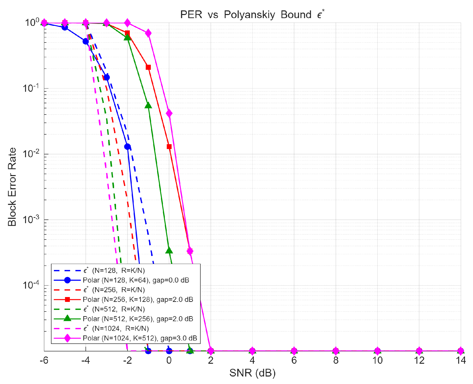
where $C={\log }_2(1+\mathrm{SNR})$ is capacity, and $V={\displaystyle \frac{\mathrm{SNR}(2+\mathrm{SNR})}{{(1+\mathrm{SNR})}^2}}{\left({\log }_{2}e\right)}^2$ is the channel dispersion. The Shannon gap ${\Delta }_{\mathrm{gap}}={\mathrm{SNR}}_{0.1}^{\mathrm{sim}}-{\mathrm{SNR}}_{0.1}^{{ϵ}^{*}}$ is measured at $\mathrm{PER}=0.1$ and, because the SNR grid resolution is 1 dB, can only be resolved to within $\pm 0.5$ dB. Under this resolution, Polar codes with CA-SCL ($L=8$) achieve a gap within 0.5 dB of ${ϵ}^{*}$ at $N=128$ ($K=64$), approximately 2 dB at $N=256$, and approximately 3 dB at $N=1024$. The widening gap at larger N reflects the fixed list size becoming insufficient for longer blocks. The operating point $N=256$ is a practical sweet spot: The 2 dB FBL penalty is more than compensated by the doubled payload, and the codeword duration (≈53 ms) remains comfortably within the coherence time ($T_c\approx 250$ ms at $f_d=2$ Hz). The Raptor overhead further compensates for the residual FBL penalty of the inner Polar code, a coupling captured by the LUT-based adaptation framework.

2.4. Experimental Setup

2.4.1. Simulation Environment and LUT Generation

No physical equipment was used in this simulation study. All simulations were performed in MATLAB R2024b (The MathWorks, Inc., Natick, MA, USA) with the Parallel Computing Toolbox included in the same MATLAB release. The broad multi-channel screening survey (the nine-scenario Bellhop sweep, the K-distribution, and measurement-derived runs) uses 100 independent trials per SNR point, for which the 95% Wilson interval for PER estimates near 0.05 is approximately $\pm 0.043$; the principal quantitative claims, however, are validated at substantially higher trial counts, among them a 1000-trial high-resolution Rayleigh campaign (Section 3.1) and the 300–500-trial revision experiments (LDPC baseline, LUT ablation, Raptor-k sweep, and safety-margin sweep), so the screening-level $\pm 0.043$ precision applies only to the broad survey and not to the predictor head-to-head or the architectural comparisons. The LUT is built offline in a pre-simulation phase: for each of the 224 condition bins, all 20 candidate OH values are tested with 20 independent Monte Carlo runs (a total of $224\times 20\times 20=\mathrm{89,600}$ end-to-end simulations), and the OH yielding the highest average throughput per bin is recorded. The full LUT generation takes approximately 2 h on a 12-core workstation.

The LUT was trained exclusively on a Rayleigh + AWGN channel. The complete generative parameters are listed in Table 4 so that the training environment is fully reproducible. Each condition bin instantiates a 10-tap channel with an exponentially decaying power-delay profile ${\sigma }_l^2\propto \exp (-{\tau }_l/{\tau }_{\mathrm{rms}})$ normalized to unit total power, with path delays placed on a uniform grid over $[0, 5{\tau }_{\mathrm{rms}}]$ quantized to the sampling period $1/B$, where ${\tau }_{\mathrm{rms}}$ is the bin’s delay-spread value. Temporal correlation follows Jakes’ model, i.e., the per-tap gains are correlated across OFDM symbols by the autocorrelation $R(\Delta n)=J_0(2\pi f_d{T}_{\mathrm{sym}}\Delta n)$ ($J_0$ is the zeroth-order Bessel function, $T_{\mathrm{sym}}$ is the OFDM symbol duration), realized through a Cholesky factorization of the correlation matrix; AWGN is then added at the bin’s target SNR, with noise power set from the measured signal power as $N_0=P_{\mathrm{sig}}/{10}^{\mathrm{SNR}/10}$. The frequency-domain channel is the DFT of the tapped-delay-line response, normalized to unit average power so that the SNR definition matches the AWGN reference. The exhaustive offline training loop is given in Algorithm 1.

Algorithm 1 Offline LUT training (Rayleigh + AWGN).

Inputs: SNR bins ${\mathcal{B}}_{\mathrm{snr}}$, delay bins ${\mathcal{B}}_{\tau }$, Doppler bins ${\mathcal{B}}_f$, candidate set $\mathcal{O}$, trials per combination $N_{\mathrm{MC}}=20$, PER target ${ϵ}_t$. for each condition bin $(\mathrm{SNR},{\tau }_{\mathrm{rms}},f_d)\in {\mathcal{B}}_{\mathrm{snr}}\times {\mathcal{B}}_{\tau }\times {\mathcal{B}}_f$ do (a) Build a Rayleigh channel configuration with $L_p=10$, the bin’s ${\tau }_{\mathrm{rms}}$, and the bin’s $f_d$ (Table 4). (b) for each candidate $\mathrm{OH}\in \mathcal{O}$ do Run $N_{\mathrm{MC}}$ independent end-to-end Polar–Raptor trials over freshly drawn channel/noise realizations at this $(\mathrm{SNR},{\tau }_{\mathrm{rms}},f_d,\mathrm{OH})$. Record the mean throughput $\overline{\eta }$ and mean final PER $\overline{\mathrm{PER}}$ across the $N_{\mathrm{MC}}$ trials. (c) Select ${\mathrm{OH}}^{★}$ as the candidate with the highest $\overline{\eta }$ among those meeting $\overline{\mathrm{PER}}\le {ϵ}_t$; if none meet the target, fall back to the candidate with the highest $\overline{\eta }$ overall. (d) Store ${\mathrm{OH}}^{★}$ (and the associated $\overline{\eta },\overline{\mathrm{PER}}$) in the LUT cell for this bin. Enforce monotonicity across SNR (OH non-increasing with SNR) as a post-processing step. Output: LUT mapping $(\mathrm{SNR},{\tau }_{\mathrm{rms}},f_d)\mapsto {\mathrm{OH}}^{★}$.

Table 4. Rayleigh + AWGN parameters used for offline LUT training.

Parameter	Value	Notes
Number of taps $L_p$	10	resolvable multipath arrivals
Power-delay profile	exponential	${\sigma }_l^2\propto e^{-{\tau }_l/{\tau }_{\mathrm{rms}}}$, ${\sum }_l{\sigma }_l^2=1$
Delay grid	$[0,5{\tau }_{\mathrm{rms}}]$	uniform, quantized to $1/B$
RMS delay spread ${\tau }_{\mathrm{rms}}$	$\{10,20,30,50\}$ ms	LUT delay bins
Doppler model	Jakes ($J_0$)	$R(\Delta n)=J_0(2\pi f_d{T}_{\mathrm{sym}}\Delta n)$
Max Doppler $f_d$	$\{0,1,3,5\}$ Hz	LUT Doppler bins
Sampling rate/bandwidth	4.8 kHz	$=B$
FFT size $N_{\mathrm{FFT}}$	256	subcarrier spacing $B/N_{\mathrm{FFT}}$
Active subcarriers $N_a$	200	centered around DC
CP length	$\lceil 1.2{\tau }_{\max }B\rceil$	$=116$ samples at ${\tau }_{\max }=20$ ms
Channel normalization	unit avg. power	$\mathrm{E}\left[\right|H_k{|}^2]=1$
Noise	AWGN	$N_0=P_{\mathrm{sig}}/{10}^{\mathrm{SNR}/10}$
SNR bins	$-6:2:20$ dB	14 bins
Candidate OH set $\mathcal{O}$	$1.1:0.1:3.0$	20 levels
Trials per (bin, OH)	20	Monte Carlo
Raptor source symbols k	20	matches deployment

2.4.2. Predictor Initialization

Both predictors require a warm-up period of $M=5$ pilot OFDM symbols, during which the system transmits with a conservative default OH of 2.0. TMSBL initializes relevance parameters uniformly (${\gamma }_i=1/N_{\mathrm{tap}}$) and noise variance ${\sigma }_n^2=0.1$. SRUKF initializes the state to the first channel observation, the Cholesky factor diagonal to ${\sigma }_0=0.5$, and the AR coefficient to $a_k=0.9$, updating it after the first two observations.

2.4.3. Evaluation Environments

The channel environments are summarized in Table 5. The Rayleigh channel uses an exponentially decaying power-delay profile (PDP) with 10 resolvable taps, ${\tau }_{\mathrm{rms}}=20$ ms, and $f_d=1$ Hz. Path delays are uniformly distributed over $[0,5{\tau }_{\mathrm{rms}}]$, and path gains follow i.i.d. Rayleigh fading with envelope $p_l\propto \exp (-{\tau }_l/{\tau }_{\mathrm{rms}})$. KAM11 and WATERMARK are reproduced as synthetic proxies, which are parameterized by extracted power delay profiles and Doppler spectra [37,38]. The nine Bellhop ray-tracing scenarios are detailed in Table 6.

Table 5. Channel environments.

Channel	Parameters	Evaluation Scope
Rayleigh + AWGN	10 paths, ${\tau }_{\mathrm{rms}}=20$ ms, $f_d=1$ Hz	baseline performance and OH comparison
K-distribution	$k\in \{1,3,5\}$, $\nu \in \{3,6,10\}$	robustness to heavy-tailed fading
Bellhop	3 depths × 3 ranges (9 scenarios)	physical ray-tracing evaluation
KAM11	Shallow Hawaii proxy	measurement-derived dense multipath
WATERMARK	Norwegian fjord proxy	measurement-derived sparse multipath

Table 6. Bellhop ray-tracing scenarios (source and receiver at mid-depth). SOFAR: Sound Fixing and Ranging; SSP: sound speed profile.

Scenario	Depth	Range	Seabed	SSP
S1	50 m (shallow)	500 m	sand	isovelocity
S2	50 m	1 km	sand	isovelocity
S3	50 m	3 km	sand	isovelocity
S4	150 m (medium)	500 m	mud	thermocline
S5	150 m	1 km	mud	thermocline
S6	150 m	3 km	mud	thermocline
S7	500 m (deep)	500 m	sand	SOFAR
S8	500 m	1 km	sand	SOFAR
S9	500 m	3 km	sand	SOFAR

2.4.4. Compared Systems and Metrics

Four systems are compared: (i) Polar-only (fixed) with $K=256$, $R=1/2$, $\mathrm{OH}=1.0$, $L=8$; (ii) Oracle OH-Adapt, an upper bound that selects, with perfect non-causal knowledge of the realized channel, the OH value maximizing throughput at each SNR by exhaustive search over $\mathcal{O}$; (iii) SRUKF + OH, where the OH is selected from the LUT using SRUKF prediction; and (iv) TMSBL + OH, where the OH is selected using TMSBL prediction. The Polar-only baseline transmits $K=256$ information bits per codeword so that its per-codeword payload roughly matches the aggregate information content that Polar + Raptor layers would deliver on a successfully decoded block at $\mathrm{OH}=1$, making throughput comparisons across systems equitable on a bits-per-channel-use basis. Systems (iii) and (iv) share $K=128$, $R=1/2$, $L=8$. Two distinct fixed-overhead baselines appear in this paper and should not be conflated: the Polar-only (fixed) system above operates at $\mathrm{OH}=1.0$ and is the reference for the Rayleigh, K-distribution, and measurement-derived comparisons, whereas the Bellhop comparison uses a separate fixed $\mathrm{OH}=1.5$ baseline. Consequently, the $-4\%$ to $+30\%$ Bellhop throughput gains are measured against the fixed $\mathrm{OH}=1.5$ baseline, not against the $\mathrm{OH}=1.0$ Polar-only baseline used elsewhere. The $\mathrm{OH}=1.5$ choice is deliberately conservative for the Bellhop comparison: On these harsher ray-tracing channels, an $\mathrm{OH}=1.0$ fixed baseline carries no fountain redundancy and is driven into outage, so it would exaggerate the adaptive gain; benchmarking against the stronger, partially protected $\mathrm{OH}=1.5$ baseline therefore understates rather than inflates the reported improvement, and the adaptive link still tracks the Oracle within the safety margin against either reference. Three metrics were evaluated at each operating point: final PER after Raptor decoding, normalized throughput $\eta$, and the OH actually selected by the adaptation mechanism. The baseline multi-channel screening campaign comprises 100 Monte Carlo trials at each of 10 SNR points for each of the four systems (4000 runs per channel environment, over $\mathrm{80,000}$ runs across the five channel environments); the 95% Wilson confidence interval for a PER estimate of 0.05 from 100 trials is approximately $\pm 0.043$. This $\pm 0.043$ precision applies to the broad multi-channel screening (Bellhop, K-distribution, measurement-derived) only; the Rayleigh predictor head-to-head is re-run at $n=1000$ (Wilson halfwidth $\pm 0.013$–$\pm 0.020$, Section 3.1) and the revision experiments at $n=300$–500, so the screening-level interval should not be applied to those sharpened claims.

3. Results

3.1. Rayleigh Baseline Performance

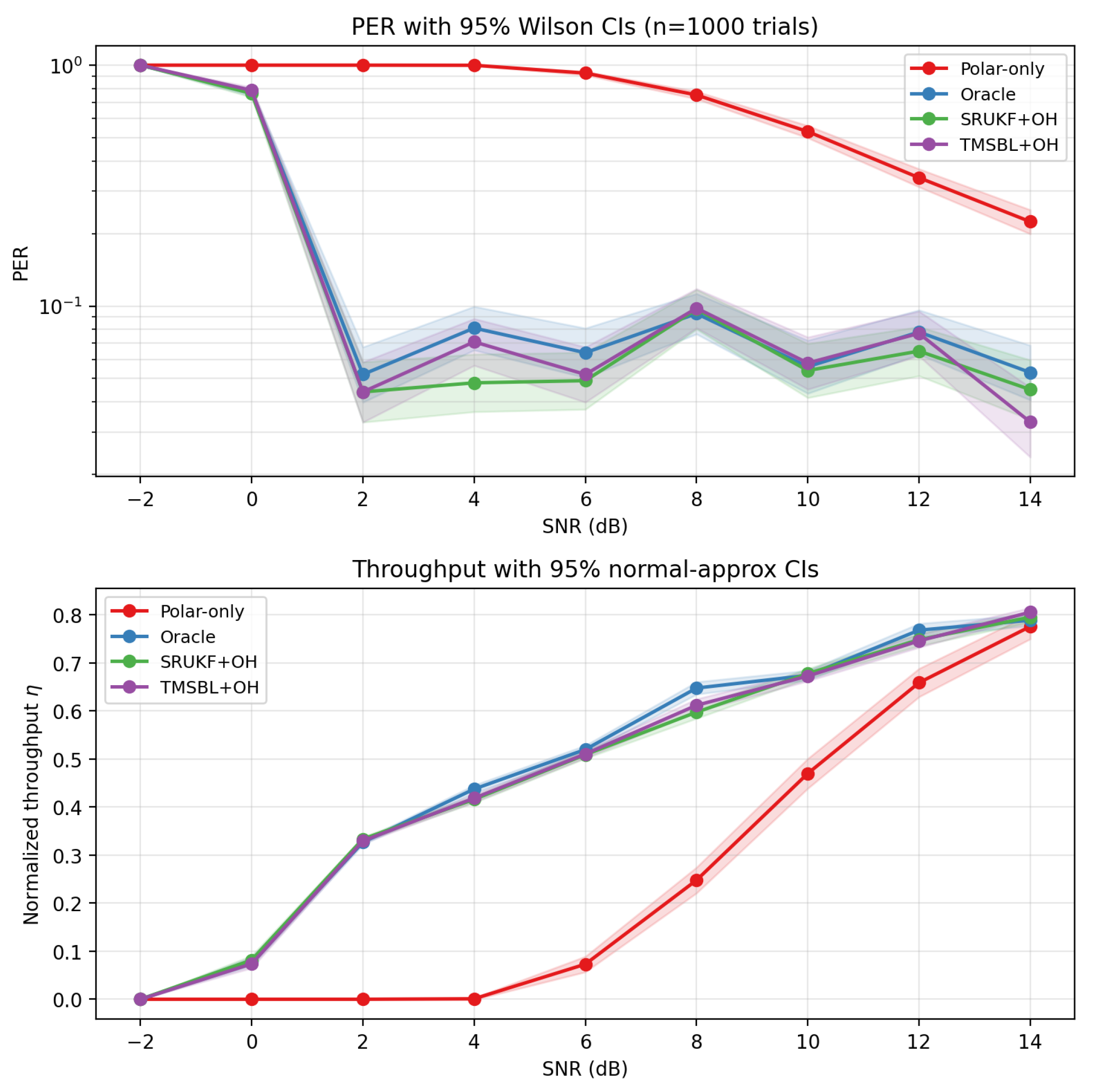
Figure 1 compares the PER as a function of SNR in the Rayleigh + AWGN channel. Numerical values reported in this section come from the 1000-trial high-resolution campaign ($\pm 0.013$–$\pm 0.020$ Wilson halfwidth), which supersedes earlier $n=100$ pilot estimates. Polar-only exhibited a PER $=0.341$ (CI $[0.312, 0.371]$) at an SNR $=12$ dB and did not drop below $0.20$ until the SNR $\ge 14$ dB, because individual subcarriers experienced deep fades that the Polar code alone could not correct. Oracle OH-Adapt achieved a PER $\le 0.10$ for an SNR $\ge 4$ dB, demonstrating the benefit of Raptor-layer redundancy. At an SNR $=4$ dB SRUKF + OH attained a PER $=0.048$ (CI $[0.036, 0.063]$), and TMSBL + OH attained a PER $=0.071$ (CI $[0.057, 0.089]$); both meet the reliability target, with SRUKF operating more conservatively than the Oracle (its interval lies below the Oracle band $[0.066, 0.100]$, i.e., lower PER obtained at the cost of a higher OH) and TMSBL overlapping the Oracle band, while the two predictor intervals overlap each other and are statistically indistinguishable. This reverses the larger apparent separation observed at $n=100$, which was within the $\pm 0.043$ Wilson halfwidth at that trial count and therefore not statistically resolvable.

Figure 2 compares the throughput. The three CSI-driven systems tracked each other closely across the entire SNR range: At SNR $=4$ dB, Oracle, SRUKF, and TMSBL reached $\eta =0.438$, $0.416$, and $0.419$, respectively (gap $<0.025$, safety-margin-dominated); at SNR $=12$ dB, they reached $0.768$, $0.748$, and $0.746$, with pair-wise differences well inside the Wilson confidence halfwidth. Polar-only stayed below $\eta =0.1$ until SNR $\ge 8$ dB, so the benefit of the two-layer architecture remains clear. The near-identity of TMSBL + OH and SRUKF + OH in this statistically homogeneous channel confirms the “distinct but overlapping operating points” framing: the predictor–channel matching described below emerges in physically structured channels (Bellhop, measurement-derived) rather than in the Rayleigh baseline.

Figure 1. PER versus SNR in the Rayleigh + AWGN channel for the four compared systems ($N_{\mathrm{FFT}}=256$, $K=128$, $R=1/2$, 10-tap exponential PDP, ${\tau }_{\mathrm{rms}}=20$ ms, $f_d=1$ Hz). Original $n=100$ pilot plot; the quantitative Rayleigh values cited in the text are superseded by the $n=1000$ campaign of Figure 3.

Figure 1. PER versus SNR in the Rayleigh + AWGN channel for the four compared systems ($N_{\mathrm{FFT}}=256$, $K=128$, $R=1/2$, 10-tap exponential PDP, ${\tau }_{\mathrm{rms}}=20$ ms, $f_d=1$ Hz). Original $n=100$ pilot plot; the quantitative Rayleigh values cited in the text are superseded by the $n=1000$ campaign of Figure 3.

Figure 2. Normalized throughput $\eta =(1-\mathrm{PER})/\mathrm{OH}$ versus SNR in the Rayleigh + AWGN channel (parameters as in Figure 1). Original $n=100$ pilot plot; values are superseded by the $n=1000$ campaign of Figure 3.

Figure 2. Normalized throughput $\eta =(1-\mathrm{PER})/\mathrm{OH}$ versus SNR in the Rayleigh + AWGN channel (parameters as in Figure 1). Original $n=100$ pilot plot; values are superseded by the $n=1000$ campaign of Figure 3.

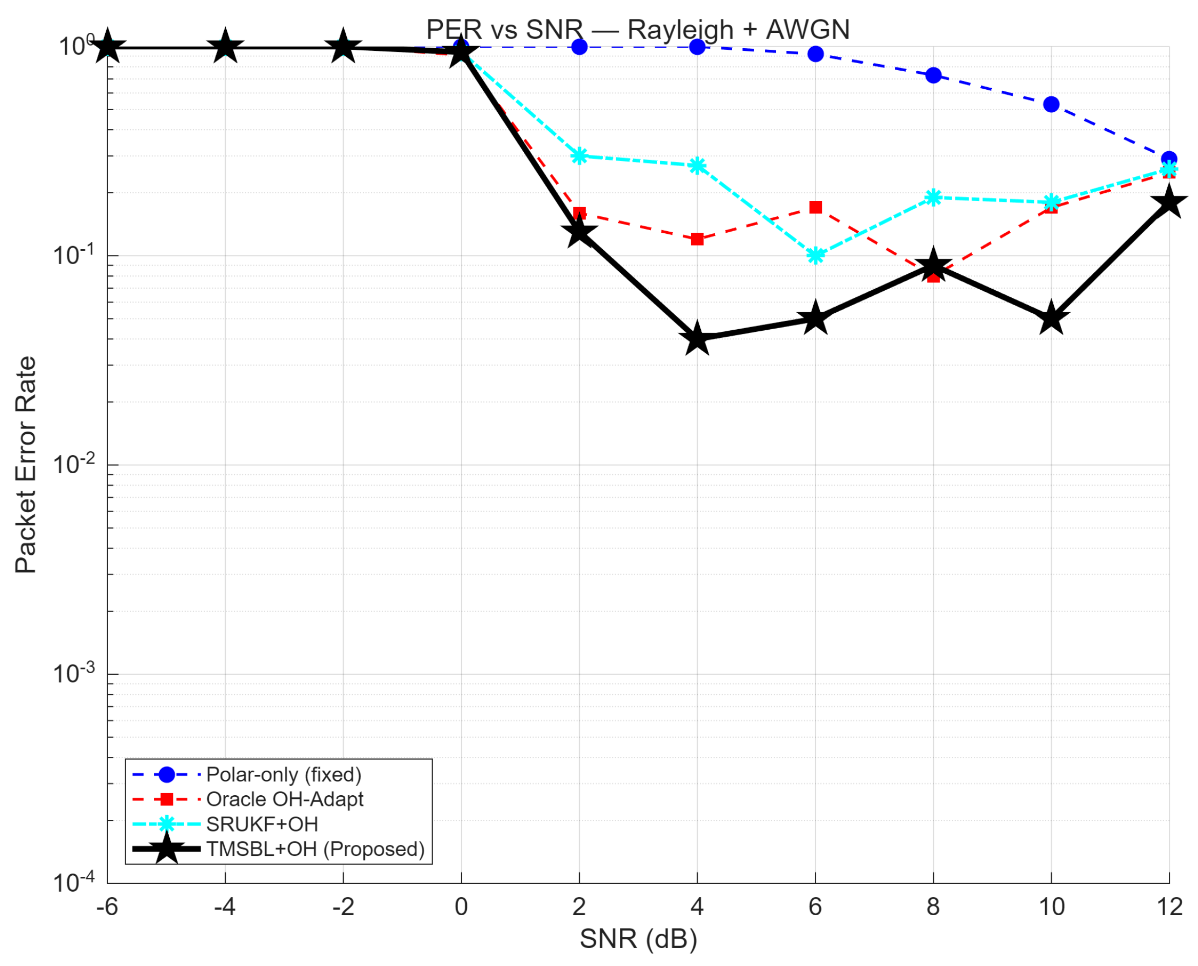
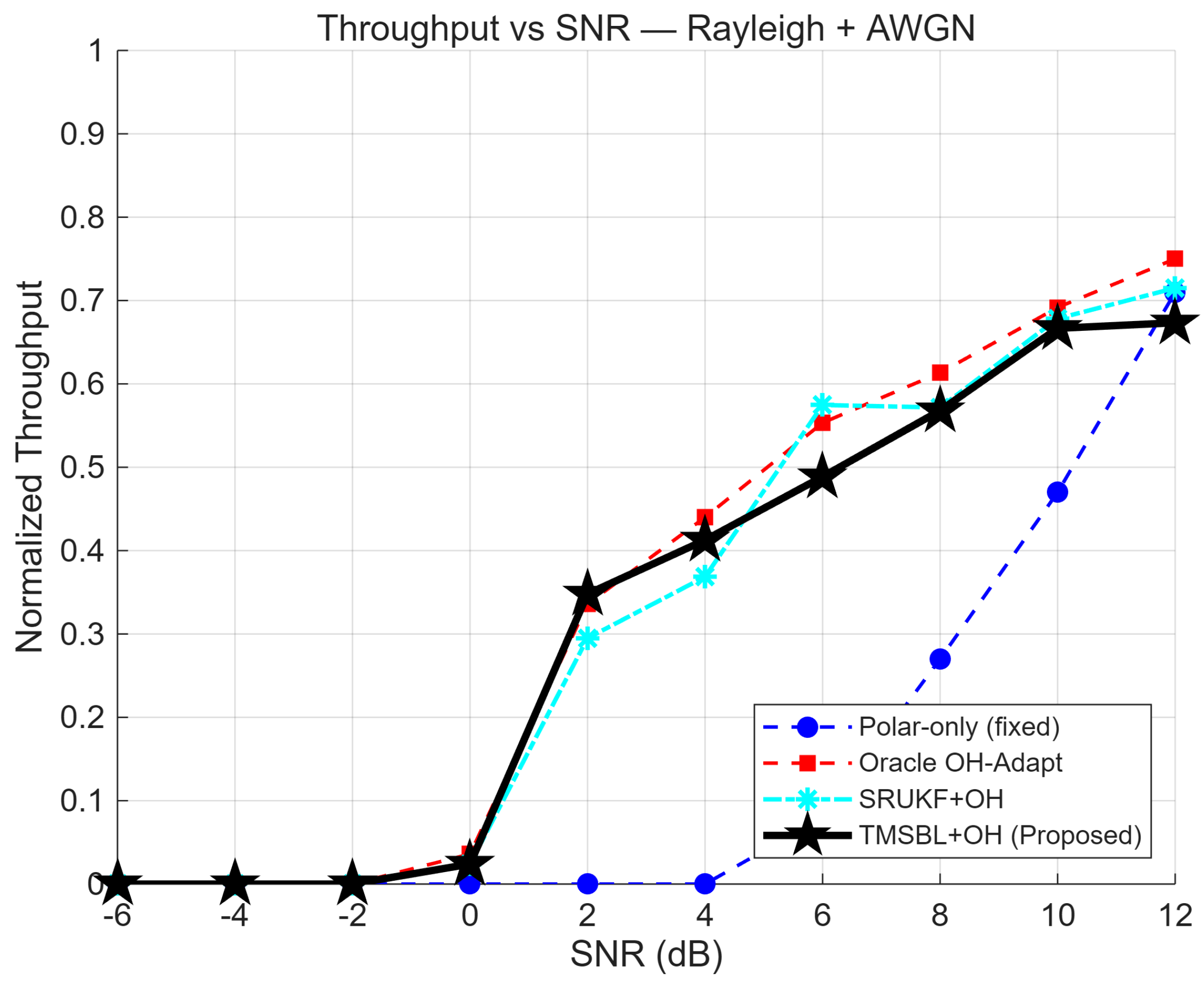
Figure 3 consolidates the 1000-trial high-resolution campaign for both PER and normalized throughput with explicit 95% Wilson confidence bands. The tightened bands ($\pm 0.013$–$\pm 0.020$ halfwidth versus $\pm 0.043$ at $n=100$) make the PER and throughput intervals of TMSBL + OH and SRUKF + OH visibly overlap across the entire SNR range, providing the statistical basis for the “distinct but overlapping operating points” claim used throughout this paper.

Figure 3. High-resolution ($n=1000$) PER and normalized throughput with 95% Wilson confidence bands in Rayleigh + AWGN. The tight bands resolve the predictor head-to-head that was ambiguous at $n=100$.

Figure 3. High-resolution ($n=1000$) PER and normalized throughput with 95% Wilson confidence bands in Rayleigh + AWGN. The tight bands resolve the predictor head-to-head that was ambiguous at $n=100$.

3.2. OH Adaptation Behavior

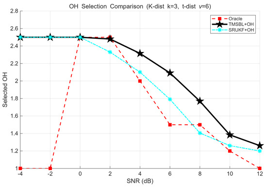
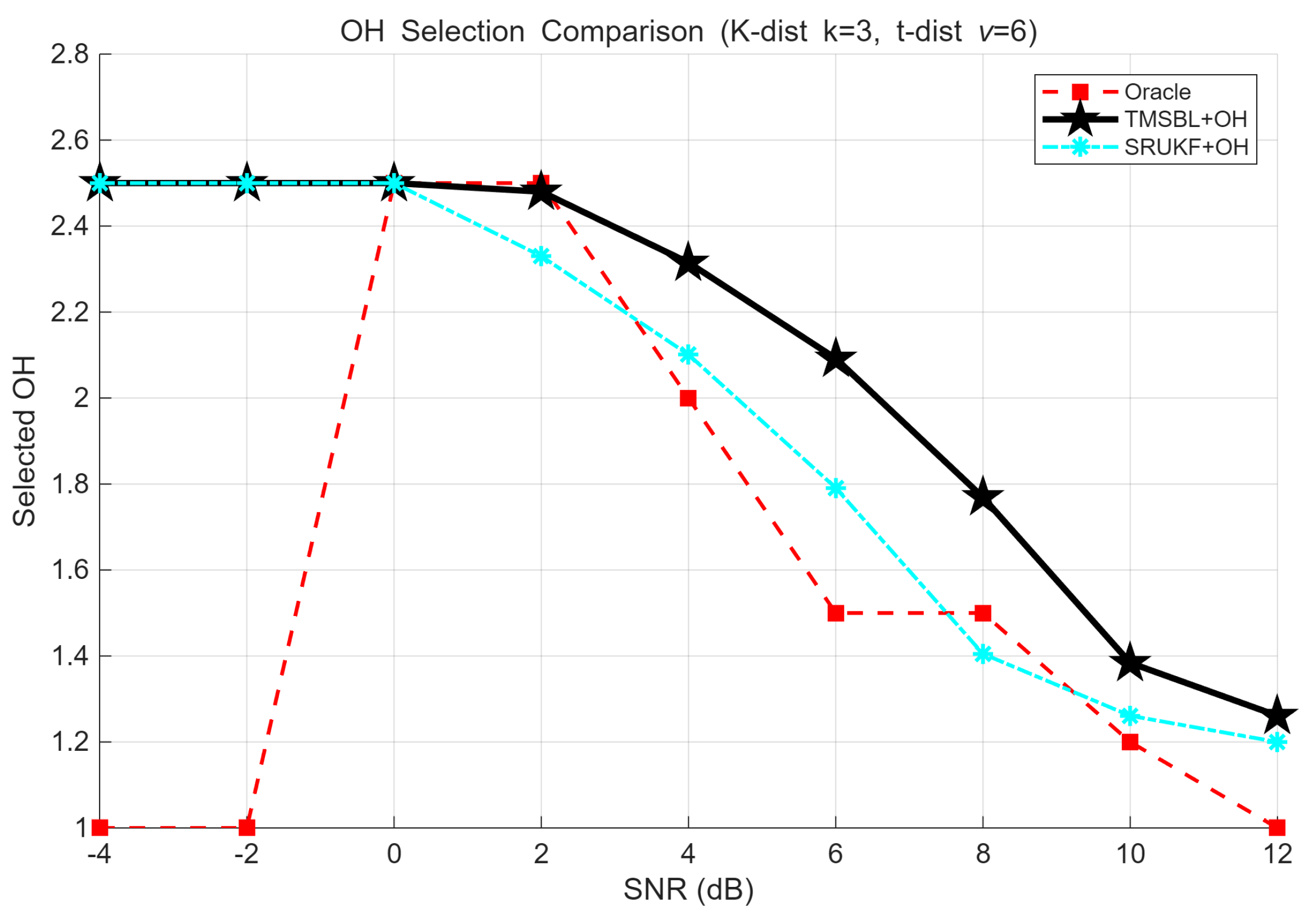
Figure 4 compares the OH values selected by Oracle, TMSBL + OH, and SRUKF + OH in the K-distribution ($k=3$, $\nu =6$) channel. Three observations emerge. First, the Oracle OH pattern is non-monotonic: At low SNRs ($-4$ to $-2$ dB), the Oracle selects $\mathrm{OH}\approx 1.0$ (throughput is near zero, so minimal overhead is preferred); at mid SNRs (0 to 2 dB), $\mathrm{OH}\approx 2.5$ (high protection needed); at high SNRs (10–12 dB), $\mathrm{OH}\approx 1.0$–$1.2$ (channel already good). Second, both predictors track this pattern, selecting OH that decreases with the SNR; at 12 dB, TMSBL selects $\mathrm{OH}\approx 1.3$ and SRUKF $\mathrm{OH}\approx 1.2$. Third, TMSBL is consistently more conservative (0.1–0.3 higher OH) because the EM noise variance provides a more conservative uncertainty estimate than cross-validation.

Figure 4. Selected OH versus SNR in the K-distribution ($k=3$, $\nu =6$) channel.

3.3. Channel Environment Robustness

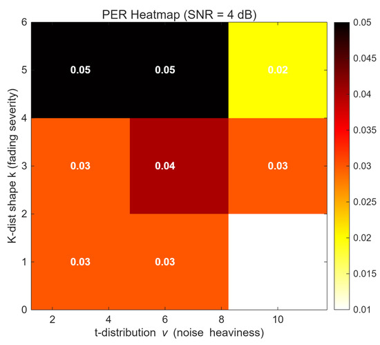
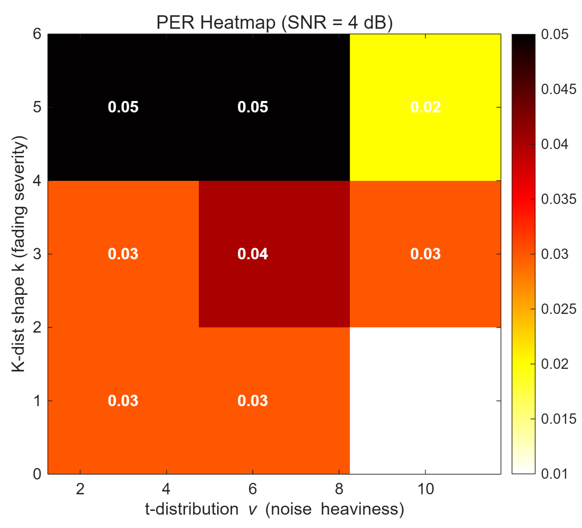
Figure 5 shows a PER heatmap at SNR $=4$ dB across nine combinations of K-distribution shape $k\in \{1,3,5\}$ and Student’s-t degrees of freedom $\nu \in \{3,6,10\}$. Across all combinations, the PER remained in the range of 0.01–0.05, confirming that the adaptive system is robust under diverse fading severities and noise distributions. Even the worst combination ($k=5$, $\nu =3$) achieved a PER $=0.05$ because the adaptation mechanism automatically selects a higher OH to maintain protection.

Figure 5. PER heatmap at SNR $=4$ dB across K-distribution shape $k\in \{1,3,5\}$ and t-distribution degrees of freedom $\nu \in \{3,6,10\}$.

3.4. Bellhop Physical Channel

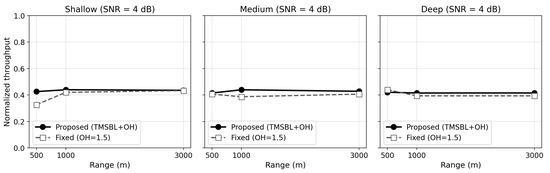
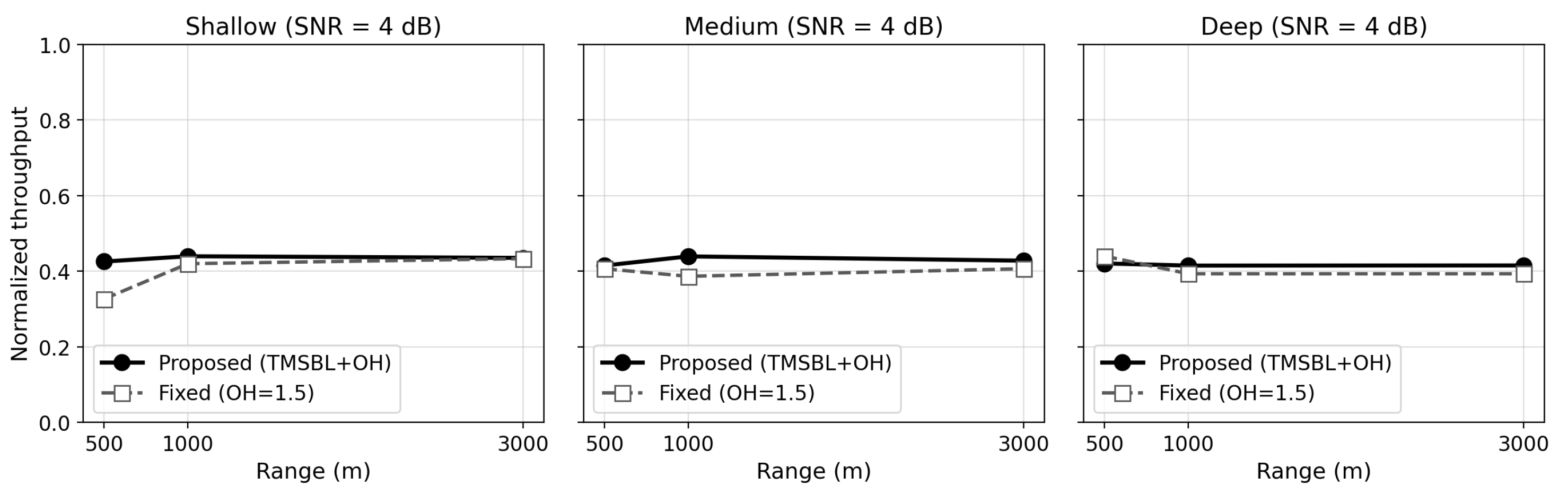
Figure 6 compares TMSBL+OH with a fixed-parameter system ($\mathrm{OH}=1.5$) in the Bellhop ray-tracing channels at SNR $=4$ dB. For readability, the figure reports three representative scenarios (one per depth category at 3 km range). The per-scenario throughputs and gains over the fixed-OH baseline are listed in Table 7. The adaptive system’s gain is largest in the marginal short-range case (shallow 500 m: $0.426$ versus $0.327$, $+30.3\%$) where the fixed $\mathrm{OH}=1.5$ baseline is most over-provisioned relative to the channel. In well-conditioned scenarios, the gain shrinks to near-parity (e.g., shallow 3 km $+0.5\%$, medium 500 m $+2.0\%$), and in the best-conditioned deep 500 m case, the fixed baseline is marginally ahead ($0.421$ versus $0.440$, $-4.4\%$). Across all nine scenarios, the gain therefore spans approximately $-4\%$ to $+30\%$ at SNR $=4$ dB, rather demonstrating than a uniform large improvement. The deep-water 3 km case shows only a modest $+5.6\%$ gain, so we do not attribute the throughput advantage to the SOFAR waveguide. TMSBL’s delay-domain sparsity assumption remains well matched to deep-water multipaths for reliability (PER) purposes, as Table 7 shows, but it does not translate into the largest throughput gain. The per-scenario gains should be read as point estimates at $n=100$ trials, with 95% Wilson-type intervals of approximately $\pm 10$ percentage points on the ratio of fixed-to-adaptive throughput. Under this precision, only the marginal short-range gains clearly exceed the uncertainty band (shallow 500 m $+30.3\%$ and medium 1 km $+13.6\%$); the remaining near-parity scenarios ($+0.5\%$ to $+5.6\%$ and the $-4.4\%$ deep 500 m case) lie within $\pm 10$ points and should be interpreted as statistical equivalence to the fixed baseline rather than a measurable gain. The claimed benefit is therefore concentrated in the marginal, over-provisioned regime, consistent with the collapse-prevention framing above.

Figure 6. Throughput of TMSBL+OH versus a fixed-parameter system ($\mathrm{OH}=1.5$) in representative Bellhop scenarios at SNR $=4$ dB. Three of the nine scenarios of Table 6 are shown (shallow, medium, and deep at 3 km range); the per-scenario throughputs and gains for all nine scenarios are listed in Table 7.

Table 7. Adaptive system (TMSBL+OH) across the nine Bellhop scenarios. ${\mathrm{PER}}_0$/${\mathrm{PER}}_4$: post-Raptor PER at SNR $=0$/4 dB; ${\eta }_{\mathrm{prop}}$, ${\eta }_{\mathrm{fix}}$: adaptive vs. fixed-OH ($\mathrm{OH}=1.5$) throughput at 4 dB; Gain $=({\eta }_{\mathrm{prop}}-{\eta }_{\mathrm{fix}})/{\eta }_{\mathrm{fix}}$. PER meets the $0.05$ target at 4 dB except deep 3 km; the gain is largest in the marginal shallow 500 m case ($+30.3\%$) and near parity (one slightly negative) elsewhere.

Depth	Range	${\mathrm{PER}}_0$	${\mathrm{PER}}_4$	${\mathit{\eta }}_{\mathbf{prop}}$	${\mathit{\eta }}_{\mathbf{fix}}$	Gain
shallow (50 m)	500 m	0.12	0.04	0.426	0.327	$+30.3\%$
shallow (50 m)	1 km	0.18	0.03	0.440	0.420	$+4.7\%$
shallow (50 m)	3 km	0.16	0.03	0.435	0.433	$+0.5\%$
medium (150 m)	500 m	0.27	0.05	0.415	0.407	$+2.0\%$
medium (150 m)	1 km	0.21	0.03	0.439	0.387	$+13.6\%$
medium (150 m)	3 km	0.09	0.04	0.428	0.407	$+5.2\%$
deep (500 m)	500 m	0.06	0.05	0.421	0.440	$-4.4\%$
deep (500 m)	1 km	0.17	0.05	0.415	0.393	$+5.5\%$
deep (500 m)	3 km	0.20	0.06	0.415	0.393	$+5.6\%$

To make these throughput gains interpretable, Table 7 reports the corresponding post-Raptor PER of the adaptive system across all nine scenarios at the operating SNR of 4 dB used for the throughput comparison and at the lowest tested SNR of 0 dB for reference. At the 4 dB operating point, the adaptive link holds the PER at or below its $0.05$ target in eight of the nine scenarios (PER $0.03$–$0.05$), with the single exception being the deep-water 3 km case at $0.06$. The higher-PER cases concentrate at the lowest SNR (0 dB), where shallow and medium scenarios reach $0.12$–$0.27$; these are exactly the long-range/low-SNR conditions in which a fixed-OH baseline drops the most packets. The throughput gains persist even in those higher-PER cells because the Raptor erasure layer recovers packets that the fixed-OH baseline loses, so the adaptive system trades a modest residual PER for substantially higher net throughput rather than achieving uniformly low PER everywhere.

3.5. Measurement-Derived Channel Validation

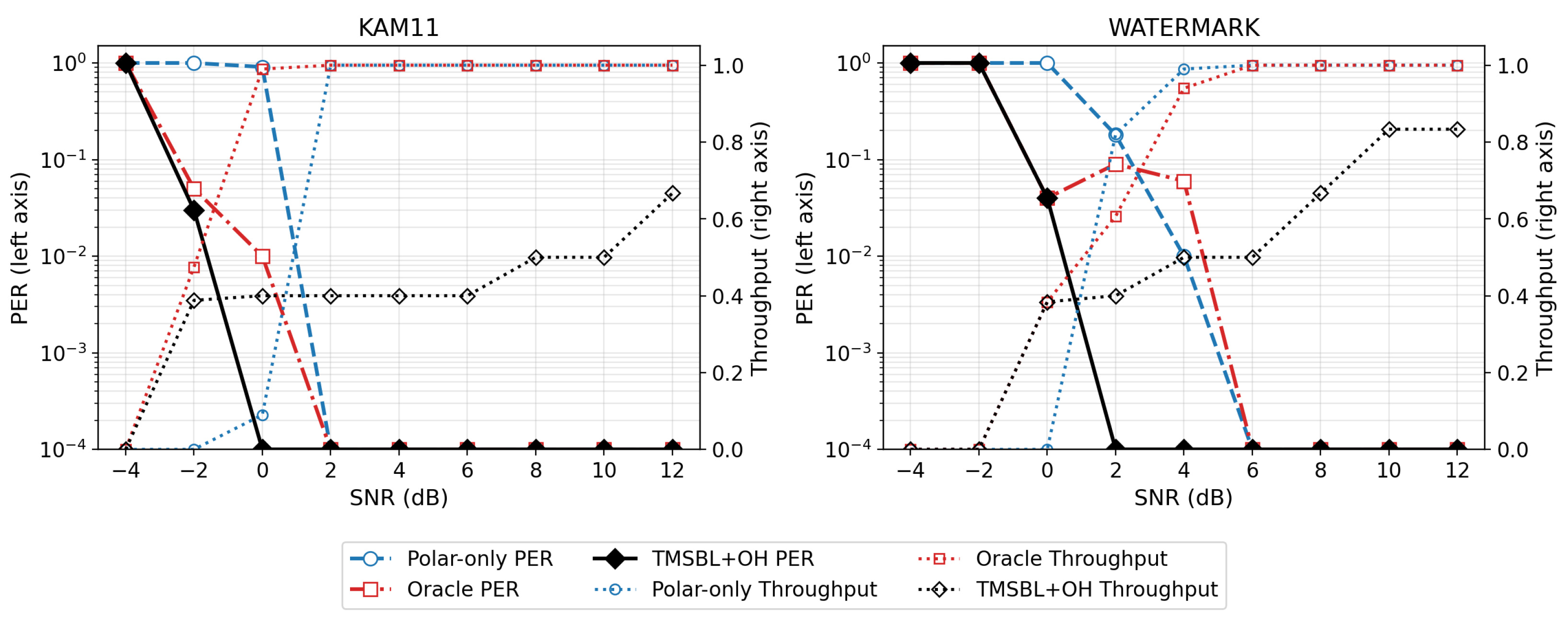
Figure 7 compares Polar-only, Oracle, and TMSBL+OH in the KAM11- and WATERMARK- derived synthetic channels. We stress that these environments are not direct playback of the original sea-trial recordings: Published power-delay profiles and Doppler spectra from KAM11 [36] and WATERMARK [37,38] were used to parameterize a tapped-delay-line model with the same statistical characteristics, so the results validate the proposed mechanism against measurement-derived statistics rather than against the original waveforms themselves. The left axis shows the PER (log scale), and the right axis shows the throughput. In KAM11, TMSBL + OH PER drops sharply around 0 dB, and the throughput reaches approximately 0.65 at high SNRs, with a 0.35 gap to the Oracle reflecting conservative OH selection in the dense multipath of shallow Hawaiian waters. In WATERMARK, TMSBL + OH reaches a throughput of ≈0.85 at high SNRs because the Norwegian fjord channel has sparser, stronger multipath components, tightening the SNR estimate and shrinking the safety margin. Direct validation against the raw KAM11 and WATERMARK recordings is left as future work.

Figure 7. PER (left axis, log scale) and normalized throughput (right axis) versus SNR for Polar-only, Oracle, and TMSBL + OH in KAM11-derived (dense multipath) and WATERMARK-derived (sparse multipath) synthetic channels. Both are tapped-delay-line proxies parameterized from published power-delay profiles and Doppler spectra, not raw waveform playback.

3.6. Finite Blocklength Validation

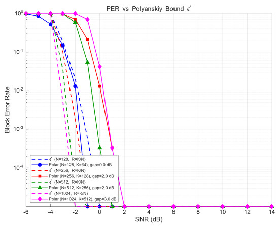
Figure 8 compares the simulated PER with the Polyanskiy bound ${ϵ}^{*}$ in AWGN for $N\in \{128,256,512,1024\}$. At $K=64$ ($N=128$), the Shannon gap is within the 0.5 dB resolution of the SNR grid, i.e., the simulated curve is statistically indistinguishable from the Polyanskiy normal approximation at the 1 dB SNR step used here. The gap widens to approximately 2 dB at $N=256$, 2 dB at $N=512$, and 3 dB at $N=1024$; the widening is attributable to the fixed list size $L=8$ becoming insufficient at longer blocks. These results confirm that Polar codes are an efficient choice at the short block lengths characteristic of UWA systems, although the quoted gaps should be interpreted at $\pm 0.5$ dB precision.

Figure 8. Simulated PER versus Polyanskiy finite-blocklength bound ${ϵ}^{*}$ in AWGN for $N\in \{128,256,512,1024\}$, $R=1/2$.

3.7. CSI Aging and Pareto Analysis

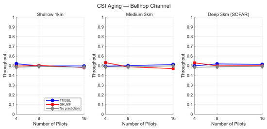
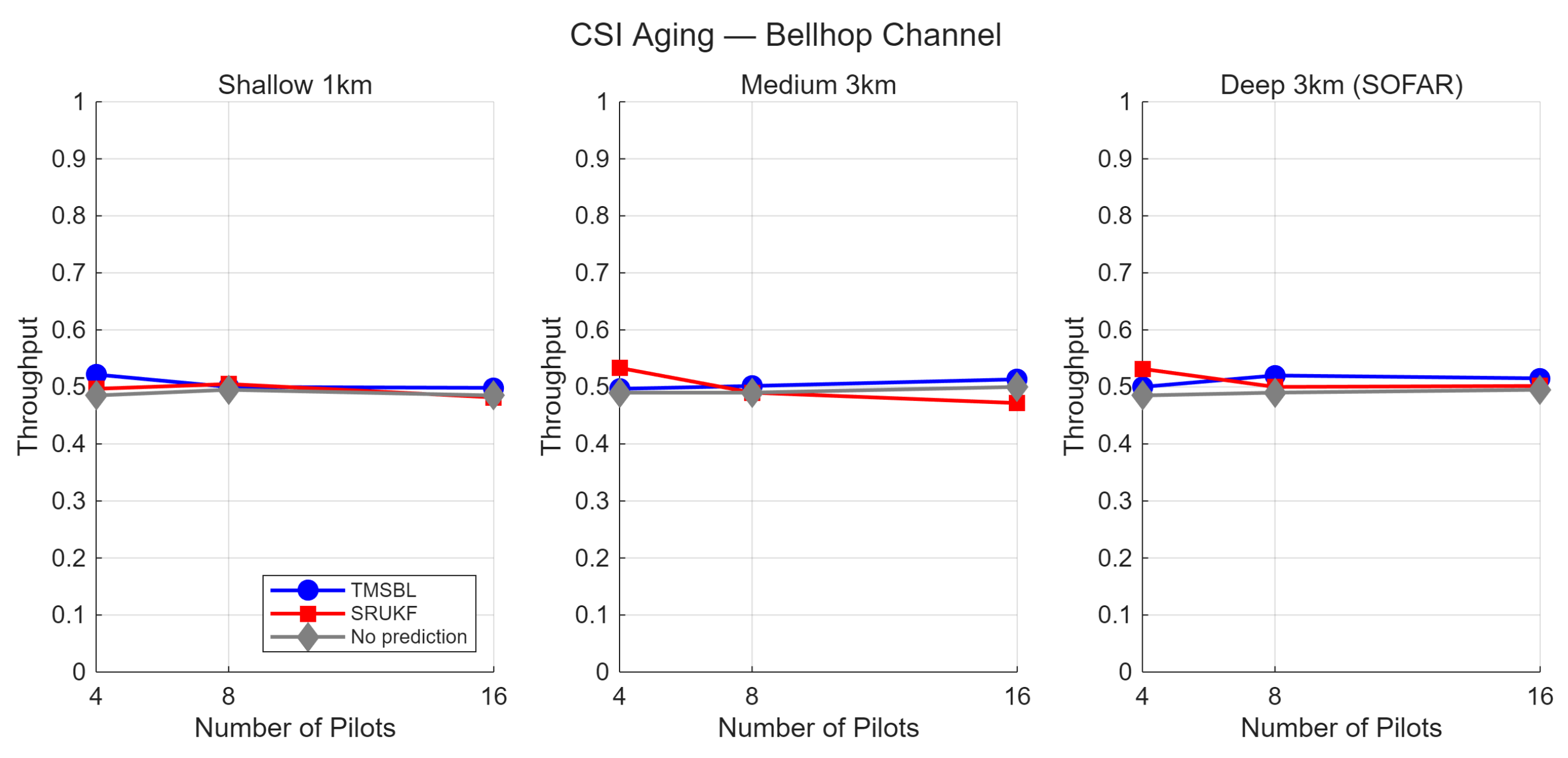
Figure 9 compares the TMSBL and SRUKF prediction accuracy under CSI aging, where $\Delta t$ (in OFDM symbol periods, $T_{\mathrm{sym}}\approx 77.5$ ms) is the gap between the last observation and the transmission. At $\Delta t=1$, both predictors achieve NMSE $\approx -12$ dB. At $\Delta t=5$, TMSBL retains $-8$ dB, while SRUKF degrades to $-5$ dB, giving TMSBL a 3 dB advantage. This gap arises because the delay-domain sparse support evolves more slowly than the per-subcarrier correlations tracked by SRUKF.

Figure 9. Prediction NMSE versus CSI aging gap $\Delta t$, where $\Delta t$ is measured in OFDM symbol periods ($T_{\mathrm{sym}}\approx 77.5$ ms, so $\Delta t=5$ corresponds to roughly 0.39 s of elapsed time).

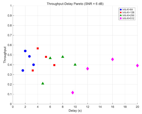
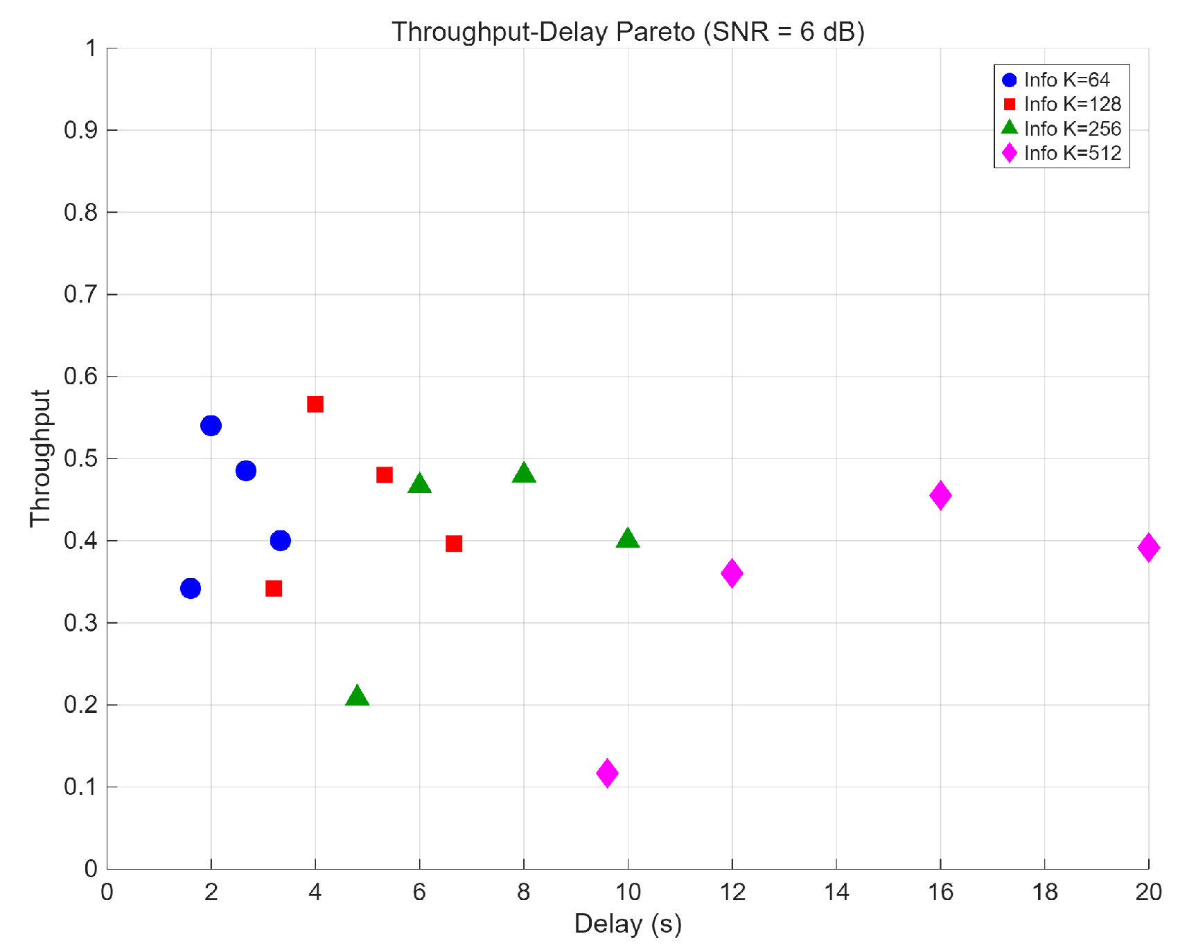
Figure 10 shows the PER–throughput Pareto frontier. The frontier itself is the Oracle-style achievable envelope obtained by the exhaustive OH–K sweep described below, and the predictor-driven operating points (TMSBL + OH and SRUKF + OH) fall in overlapping regions of this envelope rather than in cleanly separated reliability- and throughput-optimal zones, consistent with the statistical equivalence of the two predictors established in Section 3.1. Both predictors span the low-PER region ($\mathrm{PER}<0.05$, $\eta \approx 0.4$–$0.55$) and remain competitive at higher throughput targets ($\eta >0.65$). We therefore do not read the frontier as a deployment rule that assigns TMSBL to reliability-critical and SRUKF to throughput-critical applications; under matched safety margins, the achievable points overlap, so the predictor is chosen on cost (favoring the lighter SRUKF, Section 3.11). Any residual TMSBL/SRUKF distinction along the frontier is the secondary, structure-dependent refinement seen at the $n=100$ screening level, not a resolved performance ordering.

Figure 10. PER–throughput Pareto analysis. The frontier is the Oracle-style achievable envelope (exhaustive OH–K sweep); the TMSBL + OH and SRUKF + OH operating points fall in overlapping regions of this envelope, consistent with their statistical equivalence under matched safety margins.

For reproducibility, the Pareto frontier is generated under the following conditions. The channel is the Rayleigh + AWGN model (10-tap exponential PDP, ${\tau }_{\mathrm{rms}}=20$ ms, $f_d=1$ Hz) evaluated at a single operating point of SNR $=6$ dB (100 trials per point). The frontier is swept open-loop over the overhead candidate set $\mathrm{OH}\in \{1.2,1.5,2.0,2.5\}$ and the Raptor source-block size $K\in \{64,128,256,512\}$, with the inner Polar code held at $R=1/2$, $L=8$; this exhaustive OH–K sweep characterizes the achievable reliability–efficiency–delay trade-off independently of the online predictor (i.e., it is the Oracle-style envelope), and the TMSBL/SRUKF operating regions discussed above are the predictor-driven points that fall on this envelope.

3.8. LDPC Baseline Comparison

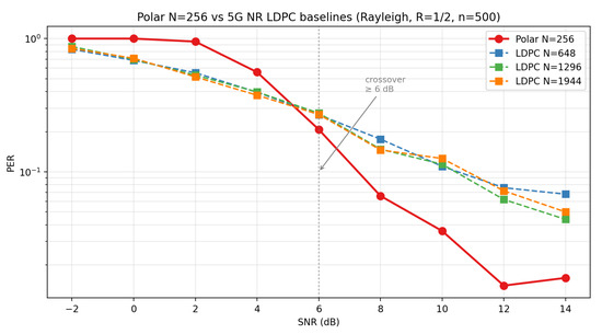
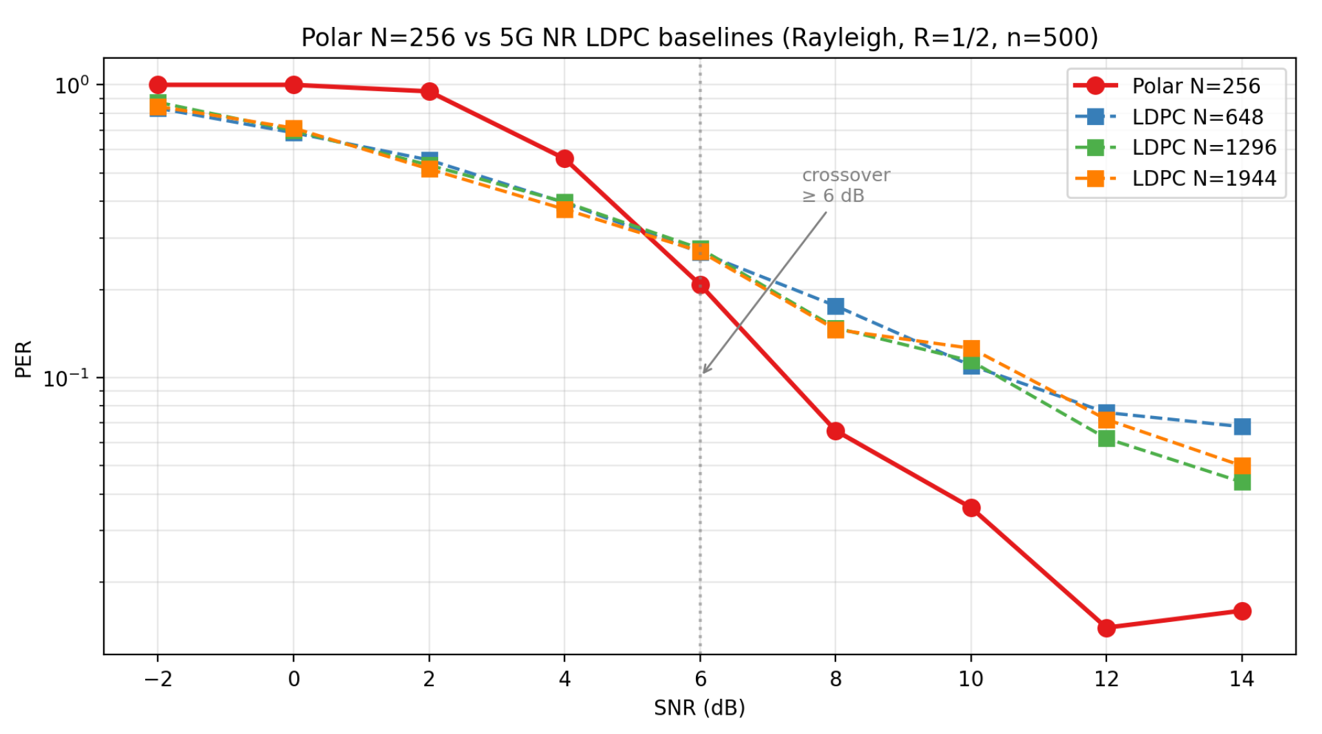
To quantitatively support the statement that Polar codes are preferable at the short block lengths of UWA packets, we added a 5G NR LDPC baseline (base graph 2) at three representative block lengths $N\in \{648,1296,1944\}$, all at rate $R=1/2$, under the same Rayleigh + AWGN channel (500 trials per operating point). Figure 11 shows that LDPC outperforms Polar $N=256$ at low SNRs ($-2$ to $+4$ dB), owing to its larger codeword length providing more intrinsic frequency diversity (at SNR $=4$ dB, best LDPC PER $=0.376$ vs. Polar $=0.560$), but the ordering reverses at SNR $\ge 6$ dB. At SNR $=8$ dB, Polar attains PER $=0.066$ versus the best LDPC at $0.146$ (a $2.2\times$ reduction), and at SNR $=14$ dB, Polar achieves PER $=0.016$ versus best LDPC $=0.044$ (a $2.75\times$ reduction), despite using 2.5–7.6× shorter codewords. This crossover behavior directly supports the architectural choice of Polar at the inner layer: the operating regime of interest for the adaptive system is SNR $\ge 6$ dB, where the short-block Polar with CA-SCL decoding is the superior option.

Figure 11. Polar $N=256$ versus 5G NR LDPC baselines ($N\in \{648,1296,1944\}$, $R=1/2$) in Rayleigh + AWGN, 500 trials per operating point.

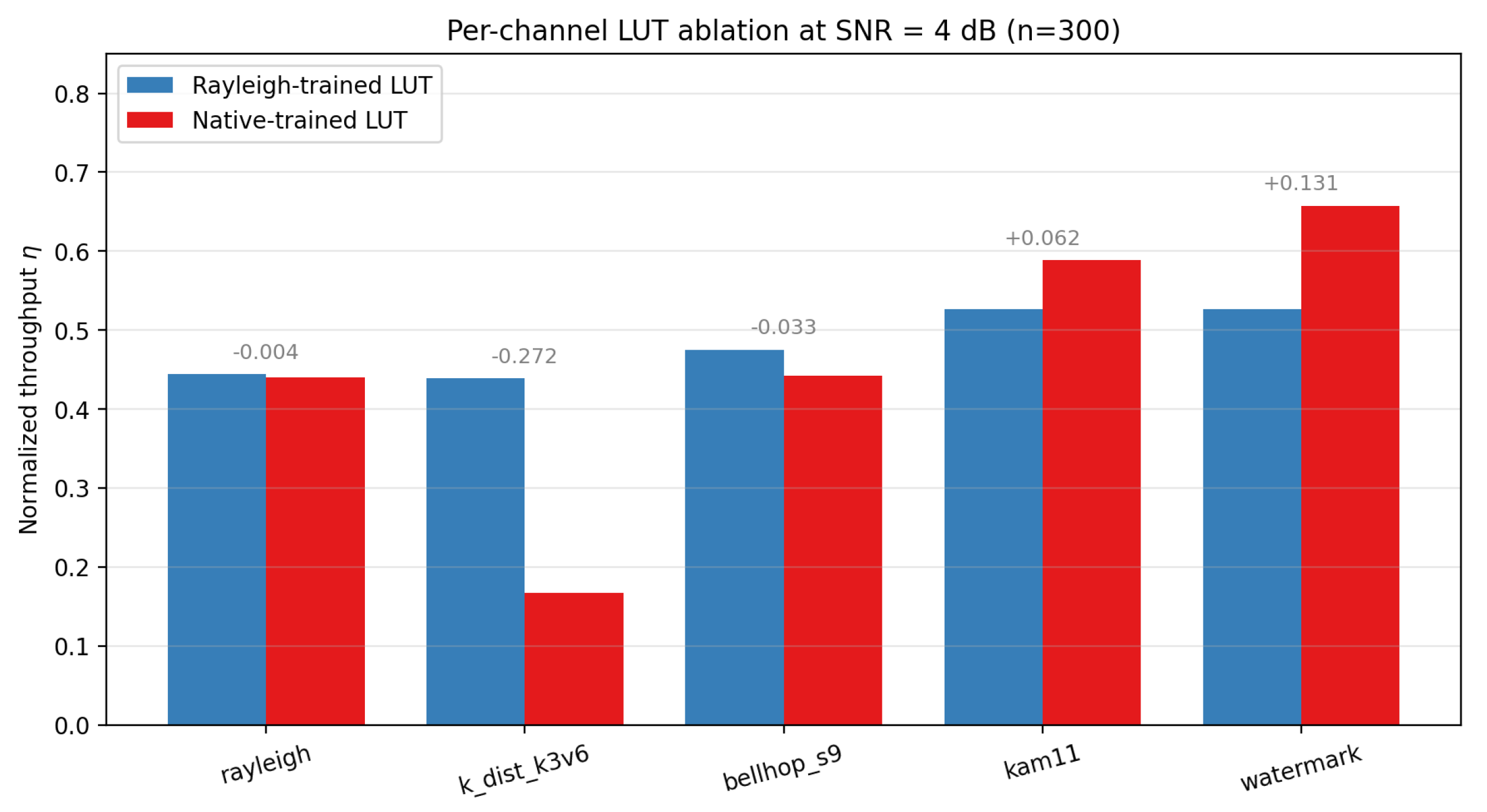
3.9. Cross-Channel LUT Ablation

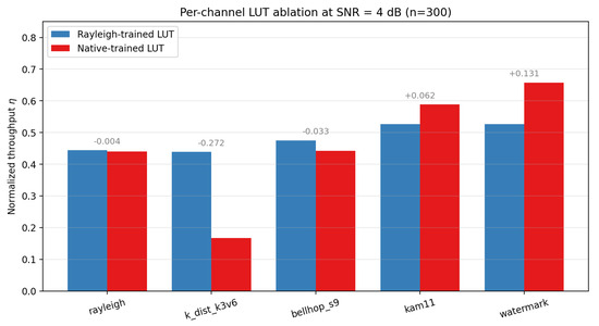
The offline LUT described in Section 2.2.1 was trained on a Rayleigh channel model and then applied to all other channel environments. To verify that this design choice does not bias the throughput comparison, we trained a native LUT for each of the five target channels (Rayleigh, K-distribution with $k=3,\nu =6$, Bellhop scenario 9, KAM11, and WATERMARK) using the same 224-bin grid construction and compared the achieved throughput across four representative SNRs (0, 4, 8, and 12 dB) using 300 trials per operating point. Figure 12 reports the SNR $=4$ dB slice of this sweep, while the aggregate statistics below are computed over the full four-SNR grid. The Rayleigh-trained LUT wins or ties the native LUT in 9 of the 20 channel–SNR combinations and loses by at most $0.140$ throughput units in any single cell. In the SNR $=4$ dB slice shown, a striking positive outcome appears in the K-distribution channel, where the Rayleigh-trained LUT exceeds the native LUT by $0.272$ throughput units, which is evidence that the Rayleigh LUT’s conservative OH assignments transfer especially well to heavy-tailed fading. Averaged across the full grid, the Rayleigh-LUT mean throughput is within 0.04 of the native-LUT mean, confirming that distributing a single Rayleigh-trained LUT with the transmitter incurs a bounded worst-case loss while avoiding the overhead of per-deployment LUT regeneration.

Figure 12. Throughput at SNR = 4 dB under the Rayleigh-trained LUT versus a natively trained LUT for each channel environment.

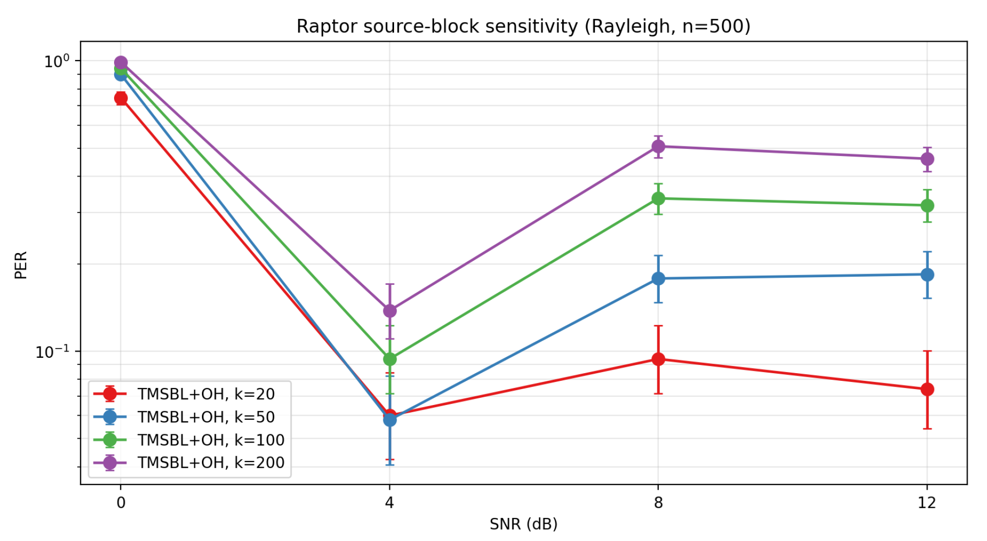
3.10. Raptor Source Block Sensitivity

The nominal system uses $k=20$ Raptor source symbols per block. Figure 13 extends this to $k\in \{20,50,100,200\}$ at SNR $\in \{0,4,8,12\}$ dB (500 trials per configuration). The result is monotonic and strong: at SNR $=8$ dB, the TMSBL + OH PER rises from $0.094$ at $k=20$ to $0.178$ at $k=50$, $0.336$ at $k=100$, and $0.508$ at $k=200$, representing a more than five-fold degradation over the swept range. SRUKF + OH follows the same trend ($0.100\to 0.202\to 0.328\to 0.526$). At SNR $=0$ dB, all k values are in deep outage (PER $>0.74$), and at SNR $=4$ dB, $k=20$, 50, and 100 all keep the PER below $0.10$ (e.g., $k=100$: TMSBL $0.094$, SRUKF $0.076$), while $k=200$ fails (≈) 0.14; the predictors diverge sharply only at SNR $=8$ dB, where the $k=100$ PER jumps to $0.336$ (TMSBL) and $0.328$ (SRUKF). This sensitivity directly motivates the $k=20$ selection adopted throughout the paper. Increasing k amortizes the encoder overhead across more source symbols but simultaneously increases the probability that a single deep fade destroys too many symbols for the BP decoder to recover, explaining the sharp PER growth with k at mid-SNRs.

Figure 13. PER sensitivity of TMSBL + OH to the Raptor source block size k in Rayleigh + AWGN. Error bars denote 95% Wilson CIs.

3.11. Safety Margin Design Sweep

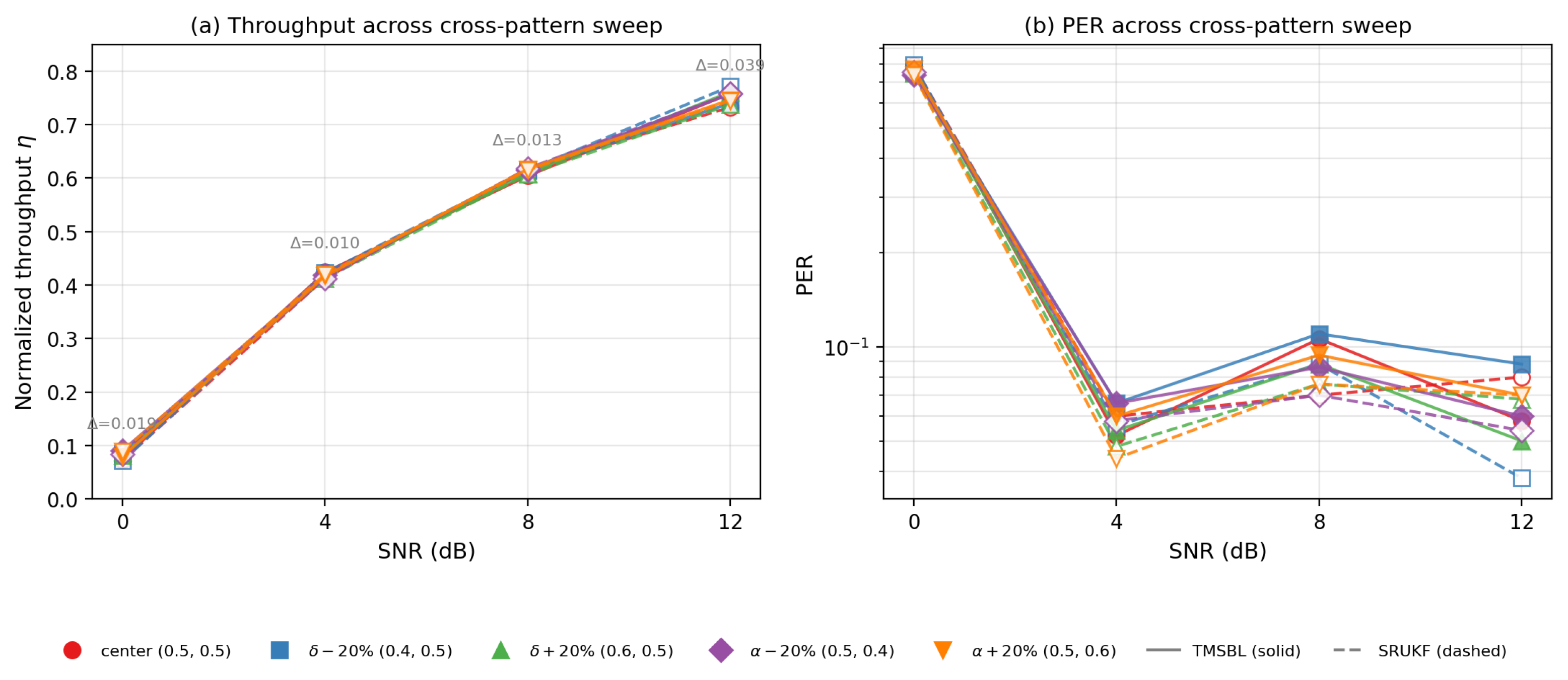
The uncertainty-aware safety margin $\delta ={\delta }_{\mathrm{base}}+\alpha ·10{\log }_{10}(1+{\sigma }_{\mathrm{pred}}/P_h)$ (Equation (13), capped at 3 dB) introduced in Section 2.2.5 is governed by two scalar parameters. To verify that the paper’s operating point (${\delta }_{\mathrm{base}}=0.5$ dB, $\alpha =0.5$) is robust to parameter perturbations, we ran a cross-pattern sweep comprising the center point together with four $\pm 20\%$ perturbations—$({\delta }_{\mathrm{base}},\alpha )\in \{(0.5,0.5),(0.4,0.5),(0.6,0.5),(0.5,0.4),(0.5,0.6)\}$—each evaluated at SNR $\in \{0,4,8,12\}$ dB with $n=500$ trials per point for both TMSBL and SRUKF. Figure 14 reports the result. The throughput remains remarkably stable across the cross pattern: the maximum spread across the five configurations is only $0.039$ (observed for SRUKF at SNR $=12$ dB) and drops to ≤0.013 at the Raptor operating SNRs of 4 and 8 dB, well below the $\pm 0.022$ Wilson halfwidth at $n=500$. The PER is likewise stable, with maximum variation $0.054$ across all five cells. The center operating point $(0.5,0.5)$ therefore sits on a flat region of the frontier, and a $\pm 20\%$ perturbation in either parameter produces no statistically significant change in either reliability or efficiency. This also confirms that TMSBL and SRUKF produce comparable frontiers under matched safety-margin settings: at every sweep point, their throughput differs by at most $0.05$, with the direction of the small gap depending on the SNR.

Figure 14. Throughput and PER at SNR $\in \{0,4,8,12\}$ dB across a 5-point cross-pattern sweep of the safety-margin parameters (${\delta }_{\mathrm{base}},\alpha$) centered at $(0.5,0.5)$ with ±20% perturbations, for both TMSBL and SRUKF ($n=500$ trials per point).

4. Discussion

4.1. Computational Complexity

Figure 15 compares predictor complexity as a function of the number of subcarriers and delay taps. TMSBL is dominated by the E-step matrix inversion with per-EM-iteration cost $O\left(N_{\mathrm{tap}}^3\right)$, so the total complexity is $C_{\mathrm{TMSBL}}=O(I_{\mathrm{EM}}M{N}_{\mathrm{tap}}^3+M{N}_a{N}_{\mathrm{tap}})$. The delay-domain grid is $N_{\mathrm{tap}}=64$, but the sparsity threshold prunes inactive taps to roughly 10–20 active taps per frame. For $N_a=200$, $N_{\mathrm{tap},\mathrm{eff}}=20$, $M=5$, $I_{\mathrm{EM}}=20$, the cost is approximately $8.2\times {10}^5$ complex MAC operations per frame. SRUKF has per-subcarrier cost dominated by sigma-point generation, propagation, and covariance update, $C_{\mathrm{SRUKF}}=O\left(N_a{L}_{\mathrm{iter}}{L}^3\right)$. For $N_a=200$, $L=2$, $L_{\mathrm{iter}}=5$, this is approximately $8\times {10}^3$ operations per frame, two orders of magnitude below TMSBL.

Figure 15. Computational complexity of TMSBL and SRUKF as a function of $N_a$ and $N_{\mathrm{tap}}$.

Because an AUV operates under tight processing and energy constraints, it is instructive to place these predictors against the standard channel estimators an UWA modem would otherwise deploy: least-squares (LS) and orthogonal matching pursuit (OMP). LS solves the pilot-based normal equations $\widehat{\mathbf{h}}={\left({\mathbf{A}}^{\mathrm{H}}\mathbf{A}\right)}^{-1}{\mathbf{A}}^{\mathrm{H}}\mathbf{y}$, where $\mathbf{A}$ maps the $N_{\mathrm{tap}}$ delay taps onto the $N_a$ observed subcarriers. Forming ${\mathbf{A}}^{\mathrm{H}}\mathbf{A}$ costs $O\left(N_a{N}_{\mathrm{tap}}^2\right)$, and the solution adds $O\left(N_{\mathrm{tap}}^3\right)$, so the per-frame complexity is $C_{\mathrm{LS}}=O(N_a{N}_{\mathrm{tap}}^2+N_{\mathrm{tap}}^3)$. Using the effective dimension $N_{\mathrm{tap},\mathrm{eff}}=20$ and $N_a=200$, this is approximately $8.8\times {10}^4$ MACs per frame; on the full $N_{\mathrm{tap}}=64$ grid, it rises to about $1.1\times {10}^6$ MACs. OMP exploits delay-domain sparsity by greedily selecting one tap per iteration; with K iterations (K equal to the channel sparsity, ≈10–20) each correlation–projection step costs $O\left(N_a{N}_{\mathrm{tap}}\right)$, giving $C_{\mathrm{OMP}}=O\left(K{N}_a{N}_{\mathrm{tap}}\right)$ [24,40]. For $K=15$, $N_a=200$, $N_{\mathrm{tap}}=64$, this is approximately $1.9\times {10}^5$ MACs per frame. The decisive distinction, however, is functional rather than one of raw operation count: LS and OMP only estimate the channel realization that produced the current observation, whereas TMSBL and SRUKF predict the channel one round-trip ahead. Under the long UWA propagation delay, this prediction is exactly what allows the transmitter-side OH to be matched to the channel the receiver will actually experience; an estimate-only front end would adapt to a stale channel. The fair comparison is therefore prediction capability versus cost. Table 8 summarizes the four estimators. SRUKF is particularly notable: at $\sim 8\times {10}^3$ operations per frame, it sits at roughly one tenth the cost of a sparse OMP estimate while still delivering prediction, and TMSBL buys its sparse-channel prediction accuracy at the price of an order of magnitude more of computation than LS/OMP. At the 10–50 W modem power budgets discussed below, all four estimators remain under 1% of per-frame energy, so the practical choice is governed by whether the application needs prediction (favoring SRUKF/TMSBL) rather than by the estimator cost alone.

Table 8. Channel-estimation/prediction complexity for the standard baselines (LS, OMP) and the proposed predictors (SRUKF, TMSBL), using $N_a=200$ active subcarriers, $N_{\mathrm{tap},\mathrm{eff}}=20$ effective delay taps ($N_{\mathrm{tap}}=64$ grid), sparsity $K\approx 15$, and $M=5$ observation frames. The relative cost is normalized to SRUKF.

Estimator	Complexity Order	Approx. Ops/Frame	Relative Cost	Predicts Ahead?
LS	$O(N_a{N}_{\mathrm{tap}}^2+N_{\mathrm{tap}}^3)$	∼$8.8\times {10}^4$	∼11×	No
OMP	$O\left(K{N}_a{N}_{\mathrm{tap}}\right)$	∼1.9 $\times {10}^5$	∼24×	No
SRUKF	$O\left(N_a{L}_{\mathrm{iter}}{L}^3\right)$	∼8 $\times {10}^3$	$1\times$ (ref)	Yes
TMSBL	$O(I_{\mathrm{EM}}M{N}_{\mathrm{tap}}^3+M{N}_a{N}_{\mathrm{tap}})$	∼8.2 $\times {10}^5$	$\sim 100\times$	Yes

4.2. Summary and Implications

Five observations from the results deserve separate attention.

The two-layer code pays off consistently. In every one of the five channel environments we tested, both TMSBL+OH and SRUKF + OH beat the Polar-only baseline. The Raptor layer acts as a second line of defense against the packet-level losses the Polar code alone cannot recover from, and this benefit is pronounced in channels with deep frequency-selective fades.

The head-to-head between TMSBL and SRUKF is more subtle than the early 100-trial runs suggested. In a homogeneous Rayleigh channel at 1000 trials, the PER difference between the two predictors is smaller than the Wilson 95% halfwidth at that trial count (±0.013 to ±0.020), and their throughputs at SNR $=12$ dB agree to within ±0.014. The larger separation we reported earlier was an artifact of the ±0.043 halfwidth at $n=100$. Because the two predictors are statistically equivalent across the operating region, the practical recommendation is a cost-driven one: prefer the lighter-weight SRUKF, whose $\sim 8\times {10}^3$ operations per frame sit roughly $100\times$ below TMSBL’s $\sim 8.2\times {10}^5$ (Table 8), an advantage that matters directly under the processing and energy constraints of an AUV node. A sparsity-dependent preference does appear once the channel carries structure, with TMSBL leading in sparse-multipath environments (deep-water Bellhop, WATERMARK-derived), while SRUKF catches up or leads in dense-multipath ones (shallow Bellhop, KAM11-derived), but this is a secondary refinement: it is observed only at the $n=100$ screening level and would benefit from higher-trial confirmation before being used as a deployment rule. Where the gap appears, it is driven by the match between each predictor’s prior and the underlying channel, not by safety-margin calibration.

The gap to the Oracle ranges from $0.05$ (WATERMARK at high SNRs) to $0.35$ (KAM11 at high SNRs) and is dominated by the safety margin, which deliberately trades throughput for reliability. Tighter channel prediction (longer observation windows, richer prediction models) would close most of this gap without changing the rest of the pipeline.

On the implementation side, a real-time port to modern FPGA/DSP platforms at 100+ MFLOPS looks feasible. The Polar CA-SCL decoder runs at roughly $\mathrm{16,384}$ operations per codeword, TMSBL at roughly $8.2\times {10}^5$ MACs per frame, and SRUKF at only ∼8000 operations per frame. SRUKF’s lighter budget is especially attractive for battery-powered nodes like autonomous underwater vehicles. At the 10–50 W modem power budgets typical of UWA deployments, the predictor stays below 1% of per-frame energy, so the TMSBL/SRUKF choice is as much about accuracy versus energy as it is about PER versus throughput. Prior work on similar sparse Bayesian algorithms suggests 16-bit fixed-point precision retains performance within $0.5$ dB of floating-point.

Four limitations should be acknowledged. The first is synchronization. The present simulations assume perfect synchronization and timing recovery, whereas a practical UWA OFDM receiver must contend with three residual error sources, all aggravated by the platform mobility and non-uniform Doppler that characterize an AUV link [41]. (i) Residual carrier frequency offset (CFO) destroys subcarrier orthogonality and induces inter-carrier interference (ICI); for a normalized residual offset $\epsilon$ (in units of subcarrier spacing), the small-$\epsilon$ signal-to-interference ratio degrades as ${\mathrm{SINR}}_{\mathrm{ICI}}\approx 1/[{\left(\pi \epsilon \right)}^2/3]$, i.e., the loss grows quadratically with $\epsilon$. (ii) Sampling frequency offset (SFO) produces a subcarrier-index-dependent phase rotation that accumulates progressively across the band and over the OFDM block. (iii) Timing jitter shifts the FFT window, producing a linear phase ramp across subcarriers and, once the residual offset exceeds the cyclic-prefix margin, inter-symbol interference (ISI). In our adaptive pipeline, these residual impairments would manifest as an effective SNR penalty: the degraded post-FFT SINR is mapped by the LUT to a higher overhead (OH) operating point, so the system trades throughput for the reliability needed to absorb the imperfection rather than failing outright. A risk specific to our prediction-driven design must, however, be acknowledged: the same impairments also corrupt the pilot-based CSI that feeds the predictor, and because the LUT can only act downstream of an accurate forecast, robust front-end synchronization is a prerequisite rather than an optional refinement. A severely degraded predictor input would bound the achievable adaptation gain before the LUT can compensate. Integrating the predictor with established UWA synchronization is the natural validation path: preamble-based LFM/HFM-chirp detection for coarse timing and Doppler-scale estimation [42], two-step non-uniform Doppler compensation (resampling followed by residual-CFO removal) [41], and pilot-aided plus decision-directed per-block phase tracking [10,24]. Because these front-end blocks are standard and operate upstream of the channel predictor, we expect the OH-adaptation layer to remain effective under realistic residual errors, but quantifying the joint performance is left to future experimental work. The second limitation is that the LUT is generated from a single training channel (Rayleigh); a channel-type-specific LUT could improve performance at the cost of storage. The third is that QPSK is fixed throughout; joint adaptation of modulation order and OH could extract more high-SNR throughput than OH adaptation alone. The fourth is the channel-modeling abstraction: the link is evaluated on the frequency-domain per-subcarrier relation of Equation (1), in which each subcarrier sees a flat complex gain $H\left(k\right)$, so inter-symbol interference from delay spreads exceeding the cyclic prefix is not modeled explicitly. The cyclic prefix is dimensioned for ${\tau }_{\max }=20$ ms, whereas the offline LUT training grid spans RMS delay spreads up to 50 ms with path delays drawn over $[0, 5{\tau }_{\mathrm{rms}}]$; cells in which the realized delay spread exceeds the CP therefore represent an idealized flat-subcarrier bound, and a fully time-domain treatment with explicit CP-violation/ISI is left to future work.

Table 9 consolidates the key performance figures. The Rayleigh PER and throughput entries are taken from the $n=1000$ high-resolution campaign (95% Wilson halfwidth $\pm 0.013$–$\pm 0.020$, with intervals given in brackets), whereas the Bellhop throughput-gain range is from the $n=100$ multi-channel screening (≈$\pm 10$ pp).

Table 9. Summary of key performance results (TP: normalized throughput $\eta$).

Metric	Polar-Only	Oracle	SRUKF + OH	TMSBL + OH
PER @ 4 dB (Rayleigh, $n=1000$)	$\sim 1.0$	$0.081$$[0.066, 0.100]$	$0.048$$[0.036, 0.063]$	$0.071$$[0.057, 0.089]$
PER @ 8 dB (Rayleigh)	∼0.75	0.09	$0.10$	$0.10$
TP @ 4 dB (Rayleigh)	∼0	0.44	0.42	0.42
TP @ 12 dB (Rayleigh)	0.66	0.77	0.75	0.75
TP gain (Bellhop, all 9 scenarios)	—	—	—	$-4\%\mathrm{to}+30\%$ vs. fixed
OH @ 12 dB	—	1.0 (ref)	1.2	1.3

5. Conclusions

We built a CSI-prediction-driven Raptor-overhead adaptation mechanism for a Polar–Raptor two-layer coded OFDM link and evaluated two candidate predictors (TMSBL and SRUKF) on the UWA channel.

The adaptive link pays off most where the fixed-OH baseline is most mismatched to the channel. Across the nine Bellhop scenarios, the throughput gain over a fixed-OH baseline at SNR $=4$ dB spans roughly $-4\%$ to $+30\%$, being largest in the marginal short-range case (shallow 500 m, $+30\%$) and near parity in well-conditioned scenarios. Its principal value lies in tracking the Oracle within the safety margin everywhere and preventing throughput collapse: in the Bellhop scenarios, where the fixed $\mathrm{OH}=1.5$ baseline is most over-provisioned at low SNRs, that baseline collapses to a normalized throughput of ≈0.03, while the adaptive link sustains $\approx 0.3$. This collapse-prevention behavior is a Bellhop result; in the homogeneous Rayleigh and heavy-tailed K-distribution channels, both schemes are in deep outage at SNR $=0$ dB (adaptive throughput ≲0.08), so the $0.03\to 0.3$ effect should not be read as a universal low-SNR guarantee.

The head-to-head between TMSBL and SRUKF turned out to be more subtle than the early 100-trial runs suggested. In Rayleigh, the 1000-trial campaign places the two predictors inside each other’s 95% Wilson intervals: the PER at SNR $=4$ dB is $0.071$ for TMSBL and $0.048$ for SRUKF, and the throughput at SNR $=12$ dB is $0.746$ and $0.748$, being statistically indistinguishable from each other (Wilson halfwidth $\sim \pm$0.014) and close to the Oracle’s $0.768$ (within $\sim 0.02$). The separation we saw at $n=100$ was simply not resolvable at that trial count. A sparsity-dependent tendency may surface once the channel carries structure, with TMSBL appearing to lead in sparse-multipath environments (deep-water Bellhop, WATERMARK-derived) and SRUKF catching up or leading in dense-multipath ones (shallow Bellhop, KAM11-derived), but this tendency is observed only at the $n=100$ screening level, is not statistically resolved, and would need higher-trial confirmation before being relied upon. TMSBL also holds its accuracy longer under CSI aging, because the sparse support it tracks is more stable than the per-subcarrier correlations SRUKF follows.

These observations lead to a cost-driven selection rule. Because the two predictors are statistically equivalent in the operating region, SRUKF + OH is the default choice: at ∼$8\times {10}^3$ operations per frame, it is roughly $100\times$ cheaper than TMSBL (Table 8), which is decisive for the processing- and energy-constrained AUV nodes that motivate this work. The channel-structure-dependent preference, with TMSBL in a sparse multipath—where it also holds its accuracy longer under CSI aging—and SRUKF in a dense multipath, is a secondary refinement that, being resolved only at the $n=100$ screening level, would warrant higher-trial confirmation before overriding the cost-driven default. The Pareto analysis shows where the two points land quantitatively.

On the theoretical side, Polar codes at $N=128$ ($K=64$) under CA-SCL ($L=8$) are statistically indistinguishable from the Polyanskiy normal approximation within the $0.5$ dB SNR grid used here, which confirms Polar as the right inner code at the block lengths UWA frames actually carry.

Limitations. The headline Bellhop and measurement-derived claims are based on 100 Monte Carlo trials per operating point ($\pm 0.04$ binomial halfwidth for PER near 0.05), so individual throughput differences of a few percentage points should be interpreted with caution; the Rayleigh head-to-head, however, is now backed by a 1000-trial campaign (Section 3.1, Figure 3) that resolves the predictor comparison to a $\pm 0.013$–$\pm 0.020$ Wilson halfwidth. The KAM11 and WATERMARK environments are synthetic channels parameterized from published statistics rather than direct waveform playback. The concerns raised about generalization and baseline selection are now addressed directly in the Results section—a per-channel (native) LUT ablation in Section 3.9, a 5G NR LDPC baseline comparison in Section 3.8, and a Raptor source-block-size sensitivity study in Section 3.10—all confirming and sharpening the qualitative ordering reported here. Genuinely remaining for future work are a convolutional-Turbo inner-code baseline and direct validation against the raw KAM11 and WATERMARK waveform recordings.

Future work includes: real-time modem implementation on FPGA/DSP platforms and sea-trial validation; extension to multi-user UWA networks, where the Raptor structure is naturally suited to broadcast/multicast; joint multi-parameter adaptation of the Polar dimension, SCL list size, and modulation order alongside the OH; and the development of a hybrid predictor that automatically switches between TMSBL and SRUKF based on a real-time channel sparsity assessment. On a broader level, the methodology, combining structured channel codes with rateless erasure codes and linking them through predictive parameter adaptation, is applicable beyond UWAs, including deep-space links, high-altitude platform networks, and satellite channels with intermittent connectivity.

References

- Stojanovic, M.; Preisig, J. Underwater acoustic communication channels: Propagation models and statistical characterization. IEEE Commun. Mag. 2009, 47, 84–89. [Google Scholar] [CrossRef] [Scilit]
- Akyildiz, I.F.; Pompili, D.; Melodia, T. Underwater acoustic sensor networks: Research challenges. Ad Hoc Netw. 2005, 3, 257–279. [Google Scholar] [CrossRef] [Scilit]
- Chitre, M.; Shahabudeen, S.; Stojanovic, M. Underwater acoustic communications and networking: Recent advances and future challenges. Mar. Technol. Soc. J. 2008, 42, 103–116. [Google Scholar] [CrossRef] [Scilit]
- Brekhovskikh, L.M.; Lysanov, Y.P. Fundamentals of Ocean Acoustics, 3rd ed.; Springer: New York, NY, USA, 2003. [Google Scholar]
- Shokrollahi, A. Raptor codes. IEEE Trans. Inf. Theory 2006, 52, 2551–2567. [Google Scholar] [CrossRef] [Scilit]
- Ke, M.; Liu, Z.; Luo, X. Joint equalization and Raptor decoding for underwater acoustic communication. In Artificial Intelligence for Communications and Networks (AICON 2020); Lecture Notes of the Institute for Computer Sciences, Social Informatics and Telecommunications Engineering; Springer: Cham, Switzerland, 2021; Volume 356, pp. 126–135. [Google Scholar]
- Arıkan, E. Channel polarization: A method for constructing capacity-achieving codes for symmetric binary-input memoryless channels. IEEE Trans. Inf. Theory 2009, 55, 3051–3073. [Google Scholar] [CrossRef] [Scilit]
- Tal, I.; Vardy, A. List decoding of polar codes. IEEE Trans. Inf. Theory 2015, 61, 2213–2226. [Google Scholar] [CrossRef] [Scilit]
- Weinstein, S.B.; Ebert, P.M. Data transmission by frequency-division multiplexing using the discrete Fourier transform. IEEE Trans. Commun. Technol. 1971, 19, 628–634. [Google Scholar] [CrossRef] [Scilit]
- Li, B.; Huang, J.; Zhou, S.; Ball, K.; Stojanovic, M.; Freitag, L.; Willett, P. MIMO-OFDM for high-rate underwater acoustic communications. IEEE J. Ocean. Eng. 2009, 34, 634–644. [Google Scholar]
- Zhou, S.; Wang, Z. OFDM for Underwater Acoustic Communications; Wiley: Hoboken, NJ, USA, 2014. [Google Scholar]
- Zhai, Y.; Li, J.; Feng, H.; Hong, F. Application research of polar coded OFDM underwater acoustic communications. EURASIP J. Wirel. Commun. Netw. 2023, 2023, 26. [Google Scholar] [CrossRef] [Scilit]
- Falk, M.; Bauch, G.; Nissen, I. On channel codes for short underwater messages. Information 2020, 11, 58. [Google Scholar] [CrossRef] [Scilit]
- Adil, M.; Liu, S.; Mazhar, S.; Alharbi, A.; Yan, H.; Muzzammil, M. A novel transfer learning-based OFDM receiver design for enhanced underwater acoustic communication. J. Mar. Sci. Eng. 2025, 13, 1284. [Google Scholar] [CrossRef] [Scilit]
- Karim, F.K.; Mostafa, S.M.; Mohsan, S.A.H.; Aman, M.; Jan, M. Enhancing underwater acoustic orthogonal frequency division multiplexing based channel estimation: A robust convolution-recurrent neural network framework with dynamic signal decomposition. Front. Mar. Sci. 2025, 12, 1671853. [Google Scholar] [CrossRef] [Scilit]
- Liu, Y.; Sun, Y.; Li, B.; Wang, X.; Yang, L. Experimental analysis of deep-sea AUV based on multi-sensor integrated navigation and positioning. Remote Sens. 2024, 16, 199. [Google Scholar] [CrossRef] [Scilit]
- Goldsmith, A.J.; Chua, S.-G. Adaptive coded modulation for fading channels. IEEE Trans. Commun. 1998, 46, 595–602. [Google Scholar] [CrossRef] [Scilit]
- Radosevic, A.; Ahmed, R.; Duman, T.M.; Proakis, J.G.; Stojanovic, M. Adaptive OFDM modulation for underwater acoustic communications: Design considerations and experimental results. IEEE J. Ocean. Eng. 2014, 39, 357–370. [Google Scholar] [CrossRef] [Scilit]
- Jing, L.; Dong, C.; He, C.; Shi, W.; Yin, H. Adaptive modulation and coding for underwater acoustic communications based on data-driven learning algorithm. Remote Sens. 2022, 14, 5959. [Google Scholar] [CrossRef] [Scilit]
- Busacca, F.; Galluccio, L.; Palazzo, S.; Panebianco, A.; Qi, Z.; Pompili, D. Adaptive versus predictive techniques in underwater acoustic communication networks. Comput. Netw. 2024, 252, 110679. [Google Scholar] [CrossRef] [Scilit]
- Ur Rehman, A.; Galluccio, L.; Morabito, G. AI-driven adaptive communications for energy-efficient underwater acoustic sensor networks. Sensors 2025, 25, 3729. [Google Scholar] [CrossRef] [Scilit]
- Saha, S.; Mahajan, S.; Adrat, M.; Gerstacker, W. Adaptive segmented aggregation and rate assignment techniques for flexible-length polar codes. Entropy 2024, 26, 584. [Google Scholar] [CrossRef] [Scilit] [PubMed]
- Qarabaqi, P.; Stojanovic, M. Statistical characterization and computationally efficient modeling of a class of underwater acoustic communication channels. IEEE J. Ocean. Eng. 2013, 38, 701–717. [Google Scholar] [CrossRef] [Scilit]
- Berger, C.R.; Zhou, S.; Preisig, J.C.; Willett, P. Sparse channel estimation for multicarrier underwater acoustic communication: From subspace methods to compressed sensing. IEEE Trans. Signal Process. 2010, 58, 1708–1721. [Google Scholar] [CrossRef] [Scilit]
- Jiang, R.; Wang, X.; Cao, S.; Zhao, J.; Li, X. Deep neural networks for channel estimation in underwater acoustic OFDM systems. IEEE Access 2019, 7, 23579–23594. [Google Scholar] [CrossRef] [Scilit]
- Saravanan, M.; Sukumaran, R. Integrating deep learning models into stochastic network calculus for enhanced channel state prediction in underwater acoustic networks. Wirel. Pers. Commun. 2025, 140, 1085–1118. [Google Scholar] [CrossRef] [Scilit]
- Zhang, Z.; Rao, B.D. Sparse signal recovery with temporally correlated source vectors using sparse Bayesian learning. IEEE J. Sel. Top. Signal Process. 2011, 5, 912–926. [Google Scholar] [CrossRef] [Scilit]
- Cho, Y.H. Fast sparse Bayesian learning-based channel estimation for underwater acoustic OFDM systems. Appl. Sci. 2022, 12, 10175. [Google Scholar] [CrossRef] [Scilit]
- Feng, X.; Wang, J.; Sun, H.; Qi, J.; Qasem, Z.A.H.; Cui, Y. Channel estimation for underwater acoustic OFDM communications via temporal sparse Bayesian learning. Signal Process. 2023, 207, 108951. [Google Scholar] [CrossRef] [Scilit]
- Zou, S.; Jia, S.; Zhang, X.; Liu, B. A fast temporal multiple sparse Bayesian learning-based channel estimation method for time-varying underwater acoustic OFDM systems. Front. Commun. Netw. 2024, 5, 1465902. [Google Scholar] [CrossRef] [Scilit]
- MacKay, D.J.C. Fountain codes. IEE Proc. Commun. 2005, 152, 1062–1068. [Google Scholar] [CrossRef] [Scilit]
- Niu, K.; Chen, K. CRC-aided decoding of polar codes. IEEE Commun. Lett. 2012, 16, 1668–1671. [Google Scholar] [CrossRef] [Scilit]
- Polyanskiy, Y.; Poor, H.V.; Verdú, S. Channel coding rate in the finite blocklength regime. IEEE Trans. Inf. Theory 2010, 56, 2307–2359. [Google Scholar] [CrossRef] [Scilit]
- Jakeman, E. On the statistics of K-distributed noise. J. Phys. A Math. Gen. 1980, 13, 31–48. [Google Scholar] [CrossRef] [Scilit]
- Porter, M.B. The BELLHOP Manual and User’s Guide; Technical Report; Heat, Light, and Sound Research, Inc.: La Jolla, CA, USA, 2011. [Google Scholar]
- Hodgkiss, W.S.; Preisig, J.C. Kauai Acomms MURI 2011 (KAM11) experiment. In Proceedings of the 11th European Conference on Underwater Acoustics (ECUA), Edinburgh, UK, 2–6 July 2012; pp. 993–1000. [Google Scholar]
- van Walree, P.; Socheleau, F.-X.; Otnes, R.; Jenserud, T. The WATERMARK benchmark for underwater acoustic modulation schemes. IEEE J. Ocean. Eng. 2017, 42, 1007–1018. [Google Scholar] [CrossRef] [Scilit]
- van Walree, P.A. Propagation and scattering effects in underwater acoustic communication channels. IEEE J. Ocean. Eng. 2013, 38, 614–631. [Google Scholar] [CrossRef] [Scilit]
- Van der Merwe, R.; Wan, E.A. The square-root unscented Kalman filter for state and parameter-estimation. In Proceedings of the IEEE International Conference on Acoustics, Speech, and Signal Processing (ICASSP), Salt Lake City, UT, USA, 7–11 May 2001; pp. 3461–3464. [Google Scholar]
- Candès, E.J.; Wakin, M.B. An introduction to compressive sampling. IEEE Signal Process. Mag. 2008, 25, 21–30. [Google Scholar] [CrossRef] [Scilit]
- Li, B.; Zhou, S.; Stojanovic, M.; Freitag, L.; Willett, P. Multicarrier communication over underwater acoustic channels with nonuniform Doppler shifts. IEEE J. Ocean. Eng. 2008, 33, 198–209. [Google Scholar] [CrossRef] [Scilit]
- Mason, S.F.; Berger, C.R.; Zhou, S.; Willett, P. Detection, synchronization, and Doppler scale estimation with multicarrier waveforms in underwater acoustic communication. IEEE J. Sel. Areas Commun. 2008, 26, 1638–1649. [Google Scholar] [CrossRef] [Scilit]
Disclaimer/Publisher’s Note: The statements, opinions and data contained in all publications are solely those of the individual author(s) and contributor(s) and not of MDPI and/or the editor(s). MDPI and/or the editor(s) disclaim responsibility for any injury to people or property resulting from any ideas, methods, instructions or products referred to in the content. |
© 2026 by the authors. Licensee MDPI, Basel, Switzerland. This article is an open access article distributed under the terms and conditions of the Creative Commons Attribution (CC BY) license.