


Highlights
What are the main findings?
- The development of a robust Kalman filter (KF)-based image fusion method using location-aware neural networks (NNs).
- A scalable recursive operation framework that can process a stream of incoming images on the fly.
What are the implications of the main findings?
- The robust KF-based image fusion method can improve robustness to measurement outliers under minimal assumption on their statistical distribution, and the proposed location-aware NNs improve estimation accuracy while reducing efforts of collecting large datasets for NN training.
- The scalable recursive operation can process images as they are observed, with a complexity that is linear in the length of the image sequence.
Abstract
Multi-resolution image fusion has been studied for years to solve the trade-off between temporal and spatial resolution in remote sensing instruments and has been widely applied to detect and monitor natural phenomena like floods. Despite the considerable research on this topic, the mitigation of the influence of outliers, such as cloud and shadow miscorrections, on satellite image fusion has not been fully developed. Moreover, strategies that integrate robustness, recursive operation and learned models are missing. In this paper, we design a robust recursive image fusion framework leveraging a location-aware neural network (NN) to model image dynamics. Outliers are modeled by representing the probability of contamination of a given pixel and band. An NN model trained on a small dataset provides accurate predictions of stochastic image time evolution, which improves both the accuracy and robustness of the method. A recursive solution is proposed to estimate high-resolution images by using a Bayesian variational inference framework. Experiments fusing images from the Landsat 8 and MODIS instruments show that the proposed method generally reduces the root mean square error (RMSE) and misclassification percentage of the estimated image by over without cloud cover and over with cloud cover compared with the benchmark KF algorithm. This indicates that the proposed approach is significantly more robust against cloud cover, without losing performance when no clouds are present.
1. Introduction
Satellite-based remote sensing is an essential tool for many applications, such as the monitoring of land-cover use [1], deforestation [2] or water quality [3]. A major concern when leveraging satellite-based imaging regards the trade-off among temporal, spatial, and spectral resolution. Such trade-off is due to the large distances between space-borne instruments and target scenes and limitations of multiband imaging systems. These limitations imply that higher spatial resolution leads to longer revisit times. For instance, the Moderate-Resolution Imaging Spectroradiometer (MODIS) has pixel sizes of 250/500/1000 m with a daily revisit period, while Landsat 8 captures images with pixel sizes of 30/100 m once every 16 days [4]. This is a major issue when monitoring events that change rapidly and at the same time require high spatial resolution to be properly characterized.
To cope with these limitations, image fusion approaches have been proposed to generate high-spatial–temporal resolution images by fusing image data from multiple space-borne instruments [5] to generate daily high-resolution (e.g., 30 m) images [6]. Spatial–temporal image fusion approaches can be divided into four categories. Unmixing-based algorithms decompose the images into the spectral signatures of the constituent materials and their pixelwise abundances, which reduces the dimensionality of the problem [7,8]. Weighted fusion predicts temporal changes in high-spatial-resolution images by using a weighted linear combination of the temporal changes in low-spatial-resolution pixels in the observed area [9]. Bayesian approaches can model the uncertainty of satellite images and further estimate high-resolution images [10,11]. Furthermore, learning-based approaches using neural networks (NNs) leverage some kind of training data to learn a mapping from low-resolution to high-resolution images [12,13]. Finally, [14] proposed SkyEyeGPT, which formulates remote sensing image understanding within a unified vision–language framework and supports diverse tasks, such as image captioning, visual question answering, visual grounding, and scene classification. These developments reflect a broader trend in remote sensing and GeoAI toward more general, language-guided, and multimodal Earth observation systems. Additionally, NNs have also been applied to other areas of image fusion; for example, [15] proposed an NN for infrared and visible image fusion based on salient target detection.
Despite the efficiency of these methods, outliers caused by effects such as cloud contamination can severely impact their image fusion performance. Thus, the detection and removal of pixels contaminated by clouds is an essential step of image fusion pipelines. Different algorithms for cloud (and cloud shadow) detection and removal have been proposed and can be divided into three categories [16]. The first kind restores cloudy/shadow-contaminated pixels by assuming that they share the same statistical distribution or geometric structures as the surrounding cloudless ones [17,18]. The second kind uses auxiliary information from different sensors, such as synthetic aperture radar [19] or MODIS images [20]. The third kind uses cloudless images from the same sensor on other dates as reference images [21].
However, the quality of cloud removal is limited, and the images used in the fusion process might still contain outliers. Thus, the development of robust image fusion methods is paramount. Moreover, although noise-robust image fusion methods have been proposed [22], there is a lack of robust online image fusion approaches.
Recursive image fusion methods process low-resolution image sequences on the fly to generate high-resolution images, benefiting from the information contained in long sequences while retaining fixed computational complexity. The Kalman filter framework [23] has been adopted in several works, as it provides a statistically principled solution to this problem. Methods based on such framework were developed to estimate time series of vegetation indices [24] and land surface temperature [10] and also to fuse Landsat and MODIS images in an offline manner [25]. A key element of this framework is a model for the time evolution of high-resolution images. This is related to a multispectral video prediction problem. Recently, a Bayesian filtering approach for image fusion was proposed in [11] using a linear and Gaussian model for image evolution, whose covariance was estimated from a small number of historical data. The flexibility of this model, however, is very limited. For computer vision, several works have proposed black-box NN-based approaches for video prediction [26,27]. However, such approaches require a large number of training data.
In this paper we propose a robust recursive image fusion framework using location-aware NNs to tackle the aforementioned limitations. The recursion is performed in the image space: at each time step k we treat the posterior distribution (represented by the fused image mean and its posterior covariance from our variational update) as the prior for the next step . In other words, we propagate and update the fused image and its uncertainty in the image space rather than in a learned intermediate feature space. The proposed recursive Bayesian formulation improves robustness and estimation quality since it can leverage temporal information and historical data, which can help to mitigate the influence of outliers (e.g., clouds) and improve robustness. By recursively updating the estimated high-resolution image, the impact of outliers (e.g., residual clouds and noise) can be reduced and estimation quality improved. In particular, the recursive process yields a statistically optimal fusion of all available information up to time k, effectively integrating information from multiple observations. Moreover, the explicit beta–Bernoulli outlier modeling yields indicator functions that down-weight or mask contaminated pixels in the likelihood, reducing their influence in the fusion process and preventing outliers from corrupting the estimated state. This yields more accurate estimates that can be updated in real time.
An illustration of the proposed method is shown in Figure 1. First, a probabilistic image acquisition model is presented in Section 2, where the measurement outliers such as clouds are represented as a statistical hypothesis of a large-magnitude outlier affecting a pixel, not requiring a rigid statistical model. Then, in Section 3 a location-aware NN-based stochastic model is proposed to represent the dynamical evolution of the high-resolution images. The NNs, which represent the mean and variance of the image evolution, are based on interpretable structures that use auxiliary variables to aid in the predictions. The NNs are trained on a small dataset of historical images of a given scene within a maximum-likelihood framework. Images from different modalities are then recursively fused in a Bayesian paradigm leveraging a variational inference framework previously developed in [28], as discussed in Section 4. To handle the high computational complexity of the Bayesian solution, a new computationally efficient distributed algorithm is developed in Section 5 by using different statistical approximations. This makes it possible to employ this solution over large datasets and geographical areas. Section 6 illustrates the experimental setup. The experimental results with real Landsat-8 and MODIS data shown in Section 7 illustrate the superior performance of the proposed approach. Section 8 discusses the proposed algorithm compared with the comparison methods, which is further concluded in Section 9.
Figure 1.
Overview of the proposed method. Time series of multimodal (e.g., Landsat and MODIS) images are recursively fused by the proposed robust Variational Distributed Multimodal Bayesian Fusion algorithm. The fused results are high-spatial–temporal-resolution estimated images, while the contamination caused by cloud/shadow influence (marked in the yellow box) is mitigated. A location-aware NN-based dynamical evolution model is estimated through a supervised strategy based on a small number of high-resolution historical data.
The proposed framework addresses key limitations of state-of-the-art algorithms, as explained in the following. For instance, ref. [22] proposes an NN-based satellite image fusion method robust against cloud influence. Despite the efficiency of this algorithm, the NN structure is complex, with about 86 convolutional layers, and the algorithm needs reference images at the preceding and succeeding times of the predicted image, meaning that it cannot be applied as an online algorithm. On the other hand, the proposed algorithm can be applied online, using only current and past observations, with NNs built using six layers in total. Similarly, refs. [29,30] propose offline NN-based satellite image fusion algorithms, but they cannot detect or mitigate cloud and shadow influence efficiently, while our proposed method can detect cloud and shadow influence directly given that it includes a robust Kalman filter. Furthermore, ref. [31] addresses clouds/outliers but does not accommodate learning/NN models, and it needs images dated a year after the processed image for better performance, meaning that it is an offline method instead of an efficient online method such as ours. Also, ref. [32] applies an online satellite image fusion method under a robust Kalman filter framework for cloud/outlier mitigation, but the dynamical model is simple and does not use all the features from the observed images efficiently. More details will be introduced for this specific comparison later in Section 2.3 as the motivation of the deep learning part of this algorithm.
In summary, the contribution of the present study is the design of a convolutional neural network (CNN)-based Bayesian variational inference framework to mitigate cloud cover influence for more accurate multi-resolution and multispectral image fusion. Furthermore, the novelty of the proposed method lies in a principled estimation framework which combines: (1) robustness to measurement outliers under minimal assumption on their statistical distribution, (2) scalable recursive operation, (3) approximated distributed implementation to reduce computational cost, and (4) integration of location-aware NNs to model image dynamics which require only a small number of training data.
2. Dynamical Imaging Model
2.1. Definitions and Notation
In this paper, we define as the k-th acquired image reflectances at the ℓ-th band with modality under , pixels for each of the bands , and as the set of image modalities. To be specific, we consider Landsat-8 and MODIS images in this paper, which are represented by . We denote the high-resolution latent reflectances by , with pixels and bands, with and , . The subindex indicates the acquisition date. Furthermore, vectorization, vector stacking, diagonal and block diagonal matrix operators are denoted by , , and , respectively. The notation for represents the set . is the Gaussian distribution, with the mean and the covariance matrix.
2.2. Measurement Model
The images acquired at each time k consist of spatially degraded, noisy versions of a high-resolution image . Following this assumption, traditional methods consider a measurement model that can be expressed according to
for each band and for each modality . The function is a linear operator representing the spectral and spatial degradation occurring at the ℓ-th band of the m-th imaging modality; it represents the effects of blurring and downsampling of the high-resolution image bands, as well as the spectral response function of the ℓ-th sensor band. is the measurement noise. Note that we assume in this paper that different bands in hold the same spatial resolution, but the resolution can be different over bands. Normally, the measurement noise is assumed as uncorrelated Gaussian noise among bands, that is, , where is the time-invariant covariance matrix for this Gaussian distribution. At each time index k, the scene is measured through one of the imaging modalities .
Using (1) and properties of the vectorization of matrix products, we can stack all bands of the m-th modality in the vector , with being the total number of pixels observed in the m-th image modality, leading to the equivalent reformulation of Model (1) as
where , , , , and is a matrix form representation of the operator , such that . denotes a vector ordering of high-resolution image , which is obtained by reorganizing all pixels to have the bands of a single high-resolution pixel, and positions corresponding to nearby pixels are adjacent to each other (see [11] for details about pixel ordering).
In satellite imaging, the pixel values can be degraded by several potential influences in the image fusion process. For example, they can be affected by the dead pixels in the sensor, atmospheric compensation error and the presence of clouds and shadow. Most existing algorithms ignore the existence of such outlier pixels, which can lead to a considerable loss of performance when they are applied in real settings. Thus, we address this issue by considering two hypotheses for the measurements. Under the first hypothesis, denoted by , the pixels are only affected by Gaussian noise , whereas under the second hypothesis, denoted by , the pixels are corrupted, being affected by a vector of outliers . This leads to the following measurement model:
for , where , and denote the i-th element of , and respectively, and denotes the i-th row of . Note that we have one hypothesis for each band and pixel in the measurement of modality m, which might be affected by an outlier. Moreover, the approach we will consider will not need a rigid statistical model for , as will be shown in the following section.
2.3. The Motivation for Using Learning-Based Dynamical Image Models
A precise model description is necessary to keep the Bayesian filtering estimation accurate. However, considering the fact that the time periods between observed images are not fixed, and the fact that the variation between pixels would change in different locations and dates, the design of a dynamical model can be a challenging task. Under the assumption that current variations in the same location can be similar to the past years, ref. [32] built a simple dynamic noise covariance estimation strategy, which is to search for the most similar images in the past and use the corresponding variation as the estimated dynamic noise covariance. There are two main limitations for this strategy: (1) the current observed image cannot be exactly the same as the historical images, and the same applies to the corresponding variation; (2) only the dynamic noise variance is estimated, while the corresponding mean value still depends fully on the measurement update phase.
To address these two limitations, we propose to use an NN to estimate both mean and variance in the dynamical model. By using the NN to extract potential features from the historical dataset instead of directly using a past variation, the dynamical model can be learned more precisely and thus leads to higher accuracy in Bayesian filtering estimation. We describe the proposed model in more detail in the following section.
3. Learning a Scene-Adapted Dynamical Model
To properly exploit the temporal information in the image sequence, an adequate dynamical model is necessary to describe the dynamics of HR images. Model-based frameworks aim to construct priors for dynamical image evolution solely based on prior knowledge, such as assuming that changes in video sequences are of low magnitude, have zero mean and are spatially smooth [33]. However, the reconstruction quality achieved using such models is limited.
Recently, the use of data-driven models has become the predominant approach to performing video prediction [34]. Such approaches are typically based on end-to-end learnable neural network architectures such as CNNs [26], recurrent neural networks (RNNs) [35] and transformers [36]. The flexibility of such models allows for accounting for long-term temporal dependencies. Stochastic models for video prediction have also been proposed to account for the uncertainty in the predictions [37]. These models are trained in a variational inference framework [38]. More recently, diffusion models have been applied to stochastic video prediction [27], owing to their great success in video generation tasks [39]. Other learning approaches leveraging physical knowledge through partial differential equations have also been recently explored [40].
For remote sensing applications, neural network models based on the transformer architecture have become well-established for forecasting tasks [41]. However, despite their flexibility, such black-box models require a large number of training data and are not easily interpretable. In [11], a simple data-driven model was proposed based on a linear and Gaussian model with a data-driven selection of an innovation covariance matrix, which needs only a small number of historical images.
Existing prediction models for videos are either black-box models which use a large number of data for training [35] or rely on analytical models [11] which are interpretable but too simplistic to properly describe the changes seen in real multispectral image sequences. To overcome this limitation, we propose a prediction model for high-resolution images based on location-aware neural networks which incorporates an interpretable architecture design. Moreover, the data-driven parts of the model, consisting of CNNs, are trained using only a small number of data consisting of a historical dataset of high-resolution images of the scene to be processed.
3.1. Supervised Dynamical Evolution Model Learning
In this section we propose to learn a scene-adapted dynamical model , which is assumed to be a conditional Gaussian distribution represented as
where vector contains additional variables used in the prediction and functions and compute the mean and the diagonal of the covariance matrix of the distribution. This corresponds to the following equivalent dynamical model:
with .
3.2. Additional Input Variables
Additional variables provide useful information for video prediction in several tasks, such as Atari games [42] or robot agents motion [43]. In remote sensing, environmental variables have been used to improve the estimation of vegetation indices from satellite data [44]. In this work, to help model the image dynamics, we consider a vector of auxiliary deterministic variables, denoted by and defined as
where denotes the date of the k-th acquisition (number of days since the first day of the corresponding year for the earliest acquisition date), is the number of days between the -th and the k-th acquisitions, is a vector containing the spatial position of each pixel, and is the variance of the image difference computed from historical data. It is inspired by the weakly supervised covariance estimation method in [11], aiming to provide a rough estimation for the average transition rate. To compute it, let us define a dataset of historical images of the scene under consideration by , with Landsat images at previous time instants. Based on , is computed as
where denotes the median time between acquisition dates of consecutive images in , which is used to normalize the result to a per-day variance estimate, and is the total number of historical images in historical dataset. The squaring in (7) is computed elementwise.
The input structure is inspired by the simple dynamic noise covariance estimation strategy in [32], where the basic idea is to find the most similar historical image and to calculate the corresponding variation among the chosen image. For this reason, and are introduced to let the NN learn the temporal features more easily. Furthermore, given that the idea is based on the assumption that variations in a certain place follow a pattern, location features are also necessary, leading to . is one of the inputs to the strategy in [32] proved to contribute to covariance estimation; therefore we also include it into the NN to provide conventional solutions as additional features.
3.3. NN Model Structure
We propose to parameterize the functions and by combining an interpretable model with CNNs learned based on the historical dataset. is given by
which is composed of the sum of the image estimate at the previous time instant and a residual computed by the CNN estimate , where represents the parameters of the CNN. denotes the rectified linear unit function, which is used to guarantee that the predicted mean is nonnegative. Note that (8) is a general expression for estimating . The diagonal of the covariance of the predictive distribution is given by
where are weighting parameters. This is a weighted combination between the variances computed a priori based on the historical dataset and a residual term computed by a CNN. The function ensures that the computed variances are nonnegative, and the result is scaled by , so that the variance becomes larger (resp., smaller) the longer (resp., shorter) the time interval between the acquisitions and k. The structure of the NNs is shown in Figure 2, where we use and to represent the neural networks generally. For details about the architecture of the NNs ( and ) and the corresponding input, please refer to Appendix A.2.
Figure 2.
Structure of the NN model used to compute the pixelwise mean and variance of the distribution of time evolution of the high-resolution images.
3.4. Cost Function
To learn the parameters of the NN-based models in (8) and (9), we consider two objectives. The main objective is to maximize the expected log-likelihood of the corresponding transition PDF , given by . When the expectation is approximated using the samples contained in the historical dataset , this leads to the following objective:
where is a constant. Note that, with a slight abuse of notation, we use to represent the set of image pairs observed at consecutive time instants in the historical dataset, with being the number thereof.
Based on , we consider the following objective function to train the neural network model:
where are regularization parameters. The first regularization term in (11), , penalizes the magnitude of weight and forces to be close to one; thus, the larger its contribution to the loss term is, the more the covariance model in (9) will approximate the a priori estimate given by , reducing the contribution of the NN. The last term, , is a weight decay which penalizes the norm of the parameters of neural networks and .
4. Robust Image Fusion Through Variational Kalman Filter
Given the probabilistic model for the image generation and its temporal dynamics, the online image fusion consists of computing the posterior distribution of the high-resolution image conditioned on all past measurements, . To simplify the notation, we will suppress the dependence of some distributions on the input variables whenever this does not impair clarity. When the model is linear and Gaussian, this PDF can be computed efficiently using the Kalman filter [11,23]. However, the proposed model tackles the presence of outliers and uses a learned temporal evolution model, which such techniques cannot address.
To address this issue, we consider an approach based on the General Variational Bayesian Kalman Filter (GVBKF) proposed in [28]. This section simply provides an overview of the proposed GVBKF presented in [28]. First, let us introduce the outlier indicator vector , such that if there is an outlier on the i-th (corrupted) element of , i.e., , and if the i-th element is otherwise clean (not corrupted). The clean elements of can be used nominally in the image fusion process, whereas the contribution of the corrupted ones should be down-weighted. This is performed by modifying the observation model such that the i-th position of the indicator vector, , adjusts the variance of a modified (referred to as improper) Gaussian noise distribution, leading to
where each element of the covariance matrix in the i-th row and j-th column is defined as for and for , where is the -th element of .
To solve the image fusion problem under the new model, we need to approximate the posterior distribution . Under the assumption of a Bayesian framework, we impose a beta–Bernoulli hierarchical prior to each indicator in , to estimate the posterior of . Specifically, we assume that is a Bernoulli distribution and follows a beta distribution, defined by (unknown) shape hyperparameters and , i.e., , for .
Note that we assume that the indicators are independent to each other in this paper. To estimate the posterior distribution of the latent variables , that is , we apply the Variational Inference (VI) principle, and resort to an auxiliary distribution using independence assumptions such that:
Then we apply the mean-field VI method to the joint distribution and acquire the various marginal distributions, ,
such that , and can be obtained by marginalizing the logarithm of the joint distribution in (14). Within the Gaussian filtering framework, the first term on the right-hand side of (14) is a predictive density, which can be approximated as , where and are the mean and covariance matrix of , which can be computed using cubature integration rules [45].
The second and third terms on the right-hand side of (14) correspond to the update phase in a Kalman filter, which can be approximated using (13), with , where and are the mean and covariance of the filtering posterior at time k, that is , while and are approximated as Bernoulli and beta distribution, respectively. To be precise, we specify term as
where follows beta distribution, defined by (unknown shape hyperparameters (notice that a beta distribution is usually defined as , where and are two shape parameters; for simplicity we omit the dependence on and and keep the form as )) and as
and is the beta function. Note that in this paper we assume that all the indicators are independent of each other:
The auxiliary distributions in (13), , and , are computed by updating them sequentially and iteratively under the Bayesian filtering scheme, defined as the GVBKF in [28]. For details of the algorithm, please refer to [28] for its full derivation and Appendix A for detailed practical setup.
5. An Efficient Distributed Algorithm
A significant limitation of the variational Kalman filter presented in the previous section is that the computation and storage requirements increase quickly with the image size, as can be attested by considering that the dimension of is quadratic in the image size. To solve this problem, we split the state into multiple groups [11]. The split groups are assumed to be statistically independent, following [46,47,48].
Note that in this section, we introduce an approximation to the distributed implementation, which is part of the novelties of this paper. It is illustrated with more details starting from Equation (23). To this end, we divide into G groups:
where the elements in each block can be regarded as dependent, but different blocks and are assumed to be independent for . Based on this assumption, the covariance matrices and can be defined as block diagonal matrices:
A natural question is which group structure should be selected. We assume a model where each block consists of all the bands of one single high-resolution pixel (resulting in blocks). Following the procedures in [46,47,48], the distributed implementation of the General VBKF under the specific independence assumption can then be derived as described in the following.
In the prediction phase of the filter, which amounts to computing the mean and covariance of , according to [47], the conditional independence assumption between groups allows us to write them as
where and denote the subset of outputs of functions and corresponding to the elements of the state vector in group g, while the notation indicates the subset of elements of vector except for those belonging to group g.
These equations involve two integrals, one with respect to the variables inside group g, which are expected to be important in the computation of the moments of group g, and another which involves the variables outside the group, which are expected to be less informative. Thus, we use two different integration schemes. In particular, the integration over is based on a cubature rule, while the integration over is based on random sampling. To generate cubature samples, we have:
where is the cubature point, for , and is the Cholesky decomposition of matrix . The random samples for variable are generated following
where , with representing the number of random samples drawn from . Following (21) and (22), the state and covariance in the distributed form are estimated as
where is the vector whose elements inside and outside group g are equal to those of and , respectively.
Since the proposed distributed General VBKF is based on the Kalman filter scheme, the distributed implementation in terms of measurement update phase is quite similar to the one in [11], while the difference appears in the Kalman filter gain and a posterior covariance, caused by the robust definition of observation covariance. The update equations are given by
where
and represents one of the possible combinations of binary values; the set of all possible combinations is given by such that . The expectation of with respect to is defined as
6. Experimental Setup
In this section, we use the proposed algorithm to fuse Landsat-8 and MODIS image sequences to generate images with high spatial and temporal resolution. We compare the proposed approach, called GVBKF-NN, to three competing recursive algorithms, illustrating the importance of both the proposed outlier and temporal evolution models. The first is a linear Kalman filter with a simple data-driven model for the dynamical image evolution proposed in [11], which we refer to as KF. The second is an extension of a Kalman filter with the learned temporal evolution model proposed in Section 3, which we refer to as KF-NN. The third is the distributed variational Bayesian fusion framework proposed in Section 4 but using the simple dynamical evolution model of [11] instead of the proposed learned dynamical model, which we refer to as GVBKF. In the following, we describe the data and experimental setup and analyze the experimental results.
6.1. Study Region
We consider two sites and two settings (cloudless and cloudy cases). The first is the Oroville Dam. It is located on the Feather River, in the Sierra Nevada Foothills (38°35.3′N and 122°27.8′W), as the tallest dam in the USA. It acts as a major water storage facility in the California State Water Project, with a maximum storage capacity of .
We focus on two particular areas of the Oroville Dam delimited by the blue and orange boxes in the left panel of Figure 3, for cloudy and cloudless cases, respectively.
Figure 3.
The left panel shows the Oroville Dam site. The blue and orange boxes delimit the study area used in the cloudy and cloudless datasets, respectively. The right panel shows the Elephant Butte site. The blue box delimits the specific study area used in the cloudy and cloudless datasets.
The other site is the Elephant Butte reservoir (Figure 3, right panel). Located in the southern part of the Rio Grande river, in NM, USA (33°19.4′N and 107°26.2′W), it is the largest reservoir in New Mexico, providing power and irrigation to southern New Mexico and Texas. It is at an elevation of 4414 ft and has a surface area of 36,500 acres. We focus on a particular area of the Elephant Butte reservoir delimited by the blue box in the lower panel of Figure 3, for both cloudy and cloudless cases.
6.2. Remotely Sensed Data
For the Elephant Butte site, we evaluated the performance of the algorithms when processing a larger geographical area of approximately 9 km × 9 km, corresponding to Landsat and MODIS images with and pixels, respectively. We focused on the red and near-infrared (NIR) bands of the Landsat and MODIS instruments since they are often used to distinguish water from other land-cover elements in the image [49]. To train and test the NNs and set up the algorithm, we collected 47 Landsat images as the historical dataset , with observed dates varying from 16 January 2014 to 24 November 2017.
In the cloudless case, after removing images with significant cloud cover between 19 March 2019 and 9 July 2019, we obtained a set of five Landsat and six MODIS images to process. The first Landsat image was used to initialize the algorithms, while two others acquired on 7 June and 23 June were set aside as ground truth to measure the performance of different algorithms. Therefore, the remaining six MODIS and two Landsat images were processed by the algorithms, and we evaluated their performance through the fused image results for 14 June and 27 June (where the MODIS observations were available), since the MODIS images from 7 June and 23 June (matching the ground truth) had to be discarded due to significant cloud cover. As for the cloudy case, the Landsat data were the same as for the cloudless case, while for the MODIS data, we substituted a clean image from 27 June with another one acquired on 19 June, which is contaminated by a cloud.
For the experiments with the Oroville Dam site, we focused on a smaller area, exploring the performance of proposed algorithms in a more extreme case, with clouds covering the whole observed area. We also evaluated the methods on the cloudless dataset of the Oroville Dam site for comparison. The study region, shown in the left panel of Figure 3, corresponded to Landsat and MODIS images with and pixels for the cloudy case (marked by an orange square) and and pixels for the cloudless case (marked by a blue square), respectively. We collected 50 Landsat data from 9 April 2013 to 7 December 2017 to serve as the historical dataset , used for training the NNs and setting up the algorithms. In this experiment we also focused on the red and NIR bands.
For the cloudless case, we collected MODIS and Landsat data acquired on the interval ranging from 3 July 2018 to 21 September 2018. After filtering for heavy cloud cover, a set of 6 Landsat and 15 MODIS images were obtained. We used the first Landsat image to initialize the algorithms. Of the remaining five Landsat images, three of them, acquired on 19 July, 20 August and 5 September, were not processed by the algorithm but only used as ground truth, while the corresponding MODIS images were used to estimate the fused image for comparison.
For the cloudy case, we collected MODIS and Landsat data acquired from 29 March 2018 to 19 July 2018. We filtered the images in this interval for heavy cloud cover, with the exception of the date 16 May 2018, for which the corresponding Landsat image is contaminated by heavy cloud cover. This led to 6 Landsat and 10 MODIS images. The first Landsat image was used as initialization for the algorithms, and two out of the remaining five Landsat images (acquired on 1 June and 3 July) were set aside for evaluation and not processed by the algorithms. They were used to evaluate the images reconstructed by the algorithms from the MODIS observations from the same dates.
6.3. Algorithm Setup
We initialized all algorithms using a high-resolution Landsat observation, i.e., , and set all the hyperparameters according to experiments performed over the historical dataset and statistics computed from it. From several tests we set the parameters of the algorithm as shown in the following.
We set , where for the Oroville Dam and for Elephant Butte, with being an all-ones matrix. For the Oroville Dam, the noise covariance matrices were set as and , where , with ⊗ denoting the Kronecker product, representing the identity matrix, and the superscript representing the adjustment of the corresponding covariance size for MODIS and Landsat images. In the Elephant Butte dataset, the noise covariance matrices were set as and , where the superscript of represents the adjustment of the corresponding covariance size for MODIS and Landsat images. The blurring and downsampling matrices were set as for Landsat, while for MODIS, is defined as a spatial convolution based on a uniform filter, defined by  (where
 matrix of ones), followed by decimation by a factor of 9 and a bandwise gain factor to compensate for scaling differences between Landsat and MODIS sensors. This represents the degradation occurring at the sensor (see, e.g., [50]).
(where matrix of ones), followed by decimation by a factor of 9 and a bandwise gain factor to compensate for scaling differences between Landsat and MODIS sensors. This represents the degradation occurring at the sensor (see, e.g., [50]).The hyperparameter of the GVBKF represents the prior knowledge of the outlier information, which is different between the two datasets. Histograms are shown in Appendix B to illustrate the difference in the outlier magnitudes between the two datasets. In this paper, and for Elephant Butte, while and for Oroville Dam. To limit the computational cost, the total number of random samples was set as for each in the distributed implementation. Further details on the setup of the proposed algorithm can be found in Appendix A.
To measure the performance of the methods, two metrics are introduced in this paper, the root mean square error (RMSE) and misclassification percentage (MP), defined as and , where represents the reference (ground truth) image with bands and pixels, represents the images estimated by the various methods, and and represent binary classification results generated by the K-means algorithm applied to and , respectively.
7. Experimental Results
7.1. Results and Discussion for the Elephant Butte Site
We fused the red and NIR bands of MODIS and Landsat for the Elephant Butte site in both cloudless and cloudy scenarios. Note that we only show the NIR reflectance band for the reconstruction result for succinctness. The results for the red band are included in Appendix B. In the cloudless scenario, the fusion results for the NIR band and all algorithms are shown in Figure 4 along with the acquired MODIS and Landsat images. In the top labels, acquisition dates represent the acquired date. If the images are processed by the fusion algorithm, we have M for MODIS and L for Landsat, following the date in the top label. As shown in the figure, only the first and last Landsat images were used in the fusion process, while the remaining two images from 7 June and 23 June act as ground truth. They are used to evaluate the accuracy of fused images from 14 June and 27 June to compare the performance of different methods (note that the MODIS images from 7 June and 23 June were not available due to cloud cover). Figure 5 shows the misclassification maps (i.e., the absolute error between the water maps by different algorithms and the ground truth). It can be seen that all four methods produce visually similar image reconstructions.
Figure 4.
Fusion results for the NIR band from MODIS (band 2) and Landsat (band 5) in the Elephant Butte cloudless case. The first two rows show the observed images at MODIS and Landsat bands. At each time index, the fused images by GVBKF-NN, GVBKF, KF-NN, KF, ESTARFM, PSRFM and EDCSTFN are presented at the following rows. Note that some Landsat images were used solely as ground truth, with only the acquisition date as the top label, while images processed by the algorithms are indicated by the top labels, where “M” stands for MODIS and “L” for Landsat.
Figure 5.
Absolute error of water map of images for the Elephant Butte example in the cloudless case based on the K-means clustering strategy. In this plot, a 0 pixel value indicates correct classification and a 1 pixel value indicates misclassification. For comparison, the acquired Landsat images are shown in the first column as the ground truth.
For comparison purposes, we include the KF, KF-NN, GVBKF, ESTARFM [9], PSRFM [51], and EDCSTFN [52] methods to estimate the fused images and compare them with the ones estimated by the proposed algorithm, GVBKF-NN. Note that all the methods except PSRFM methods, including the proposed one, are online methods, which only estimate the fused images based on the current and past observations. However, PSRFM is an offline algorithm which not only depends on the current and past observations but also on future observations; thus, it is included only as a reference which illustrates what performance can be achieved if more measurement information is available. The acquisition of more information makes offline methods hold the best performance in theory in the normal case [23], but not under outlier influence, and it will be shown in the following experimental results.
To evaluate the performance of different methods more clearly, we introduce RMSE and misclassification percentage as our metrics. RMSE is a widely used metric for evaluating image fusion performance, and it is listed in references such as [53,54]. The misclassification performance metric is also a widely used performance metric for image fusion, as it is less sensitive to variability effects such as illumination differences which can affect the RMSE; it has been considered in impactful works such as [55,56]. In Table 1, the misclassification percentage and the RMSE of the estimated images are provided. In terms of RMSE, the GVBKF-NN and the KF-NN show close performance on average. The GVBKF and the KF, on the other hand, show higher RMSE. Furthermore, we have the conventional method ESTARFM and an NN-based method EDCSTFN, which have even higher RMSE because they rely on only one or two pairs of observed images, instead of all observed images from the past to the present like the recursive algorithms listed above. Note that the PSRFM has the smallest RMSE, and that is because this method takes advantage of both observed images before and after the current time step. In other words, the PSRFM is an offline algorithm, and we can still say that the proposed algorithm performs the best among the online algorithms applied. Furthermore, in terms of the uncertainty estimates, which is the posterior standard deviation of the estimated solution in the KF-based algorithms, we can see that the ones with an NN (KF-NN and GVBKF-NN) have a much tighter bound than the ones without an NN (KF and GVBKF), which indicates the contribution of NNs to precise model description clearly. In terms of misclassification percentage, we can see that the GVBKF-NN holds the smallest misclassification percentage on average among methods, except the offline PSRFM method, and the second best method is the KF-NN, followed by the KF, the GVBKF, the EDCSTFN, and the ESTARFM. This shows that the NN model is important for preventing performance losses in the proposed robust framework in the absence of outliers. Specifically, if we compare the proposed GVBKF-NN with the KF, the advanced Bayesian filtering method with its prototype, the RMSE is reduced by on average, and the misclassification percentage is reduced by on average.
Table 1.
Misclassification and RMSE performance for the Elephant Butte site in the cloudless scenario.
In the cloudy scenario, the fusion results for the NIR band and all algorithms are shown in Figure 6, while Figure 7 shows the misclassification mappings. To compare different methods with the proposed one, the Landsat images from 7 June and 23 June act as ground truth to measure the accuracy of fused images for 14 June and 27 June (the MODIS images from 7 June and 23 June were not available due to cloud cover). Note that in the MODIS dataset, on 19 June, part of the pixels in the top part are covered by a cloud. It can be seen that the ESTARFM is heavily influenced by the cloudy image, followed by the EDCSTFN, the KF, and the GVBKF. The cloud in the images estimated by those methods for 19 June is basically not removed at all, while the cloud in the image processed by the PSRFM is removed a bit, but there is still some left. The proposed GVBKF-NN, on the other hand, is able to suppress the outlier, while the KF-NN shows intermediate performance. This indicates that the robustness of the outlier-aware variational inference framework against cloudy pixels depends on the accuracy of the dynamical image evolution model and shows that considering both the robust methodology and the learned NN evolution model is key to obtaining high performance with the GVBKF-NN approach.
Figure 6.
Fusion results for the NIR band from MODIS (band 2) and Landsat (band 5) for the Elephant Butte example in the cloudy case. The first two rows show the observed images at MODIS and Landsat bands. At each time index, the fused images by GVBKF-NN, GVBKF, KF-NN, KF, ESTARFM, PSRFM and EDCSTFN are presented in the following rows. Note that some Landsat images were used solely as ground truth with only acquisition date as top label, while images processed by the algorithms are indicated by the top labels, where “M” stands for MODIS and “L” for Landsat.
Figure 7.
Absolute error of water map of images for the Elephant Butte example in the cloudy case based on the K-means clustering strategy. In this plot, 0-valued pixels indicate correct classification, and 1-valued pixels indicate misclassification. For comparison, the acquired Landsat images are shown in the first column as the ground truth.
The quantitative results are shown in Table 2, which contains the misclassification percentage and the RMSE of estimated images of the different methods. The GVBKF-NN and the KF-NN show the first- and second-best performance on average in terms of both misclassification percentage and RMSE among the online algorithms. The GVBKF and the KF, which do not have an accurate dynamical evolution model, show significantly worse performance. For the offline method, although the PSRFM method performs the best, it cannot avoid cloud influence on 19 June, leading to higher RMSE and misclassification compared with the GVBKF-NN for the same date. Furthermore, in terms of the uncertainty, the KF-NN and the GVBKF-NN still hold a tighter bound than the KF and the GVBKF, showing that the contribution of the NN to precise model description is not influenced by clouds and shadow. Specifically, comparing the proposed GVBKF-NN with the KF, the RMSE is reduced by on average, and the misclassification percentage is reduced by on average. In summary, the results for Elephant Butte have showed that the learned NN-based model, by representing the image evolution more accurately, brings about important improvements to both the GVBKF and KF methods.
Table 2.
Misclassification and RMSE performance for the Elephant Butte site in the cloudy scenario.
7.2. Results and Discussion for the Oroville Dam Site
We now compare the four algorithms on the Oroville Dam case with and without clouds. The setup is similar to the one for the Elephant Butte example. Considering space limitations, only quantitative results are provided. Please refer to the supplemental material for the reflectance and water mapping results. For the cloudless scenario, Table 3 shows the misclassification percentage and the RMSE of the images estimated by the different methods when they were compared with the ground truth. It can be seen that among the online methods, the GVBKF-NN has the smallest RMSE and misclassification percentage on average, while the second-best method is the KF-NN, followed by the GVBKF and the KF. The PSRFM method has the smallest RMSE and misclassification percentage, but it is not fair to compare an offline method with online methods, which take advantage of images observed in both the past and the future. Furthermore, in terms of the uncertainty estimates, we can see that the KF-NN and the GVBKF-NN have a much tighter bound than the KF and the GVBKF, following the pattern we observed in Elephant Butte. Specifically, comparing the proposed GVBKF-NN with the KF, the RMSE is reduced by on average, and the misclassification percentage is reduced by on average. Like in the Elephant Butte example, this illustrates the performance improvements brought about by the use of the proposed temporal image evolution model based on NNs when no outliers are present.
Table 3.
Misclassification and RMSE performance for the Oroville Dam site in the cloudless scenario.
We also evaluate the methods in the cloudy scenario, when the Landsat image from 16 May is completely covered by a large cloud present over the observed area, constituting a more extreme case of outlier contamination. Note that since there is no cloudless Landsat image around 16 May available for use as ground truth, we used the interpolation method to estimate a surrogate ground truth of the Landsat image from 16 May from the Landsat observations from 14 April and 1 June. The quantitative results are shown in Table 4, where the results at 16 May are based on the ground truth obtained by the interpolation method. It can be seen that the results estimated by the KF, the ESTARFM, the EDCSTFN, and even the PSRFM method are heavily influenced by the large cloud cover in the Landsat observation from 16 May. On the other hand, the GVBKF, KF-NN and GVBKF-NN methods exhibit comparatively stable performance, keeping estimated images robust against large cloud cover. Specifically, the GVBKF-NN outperforms the other methods on average, followed by the GVBKF and the KF-NN, which showed similar performance. The KF had the worst performance by far. Additionally, the KF-NN and the GVBKF-NN still have a much tighter uncertainty bound than the KF and the GVBKF.
Table 4.
Misclassification and RMSE performance for the Oroville Dam site in the cloudy scenario.
This illustrates the advantages of combining both the robust framework and the learned NN-based model. Specifically, in the presence of an extreme number of outliers in the image, the robust methodology of the GVBKF is able to provide more competitive performance and mitigate the presence of outliers with the KF-NN even without an accurate evolution model. To be detailed, comparing the proposed GVBKF-NN with the KF, the RMSE is reduced by on average, and the misclassification percentage is reduced by on average.
8. Discussion
This paper develops a robust multimodal multispectral satellite image fusion algorithm, aiming to mitigate the influence of clouds and shadow. The proposed algorithm is based on Bayesian filtering, utilizing information of images observed from past to the current time. For this reason, all Bayesian filtering methods (KF, KF-NN, GVBKF, and GVBKF-NN) outperform conventional methods (e.g., ESTARFM), as shown in Table 1, Table 2, Table 3 and Table 4, in terms of both RMSE and misclassification percentage. Furthermore, to improve the accuracy of model description, an NN is designed as a dynamical model to estimate the mean and covariance of the state vector. This is validated by the fact that the KF-NN and the GVBKF-NN show smaller RMSE and misclassification percentage than the KF and the GVBKF, respectively, as shown in Table 1, Table 2, Table 3 and Table 4. Furthermore, according to the tables, the GVBKF-NN and the KF-NN provide a tighter bound in terms of the uncertainty calculation, indicating the NN’s higher dynamical model description accuracy compared with the conventional one.
The PSRFM method provide the smallest RMSE and misclassification percentage in Table 1 and Table 3 in the cloudless scenario, because it utilizes information from images observed in the past, current time, and future. This means that the PSRFM method is an offline method and cannot applied to real-time satellite image fusion, while our proposed algorithm does not have this limitation. Additionally, according to Table 2 and Table 4, the PSRFM has no robustness against potential cloud and shadow influence, which is another advantage of our proposed algorithm.
Furthermore, a distributed implementation is applied, as introduced in Section 5, to control the computational cost of Bayesian filtering-based algorithms. It allows for a scalable operation of the proposed algorithm without worrying about computational efficiency. The proposed NN is simple and needs a small dataset, meaning that the algorithm can be applied even though the historical dataset of the targeted area is limited, which further improves the practical use of the proposed algorithm.
9. Conclusions
In this paper, we proposed a recursive image fusion method based on location-aware NNs that is robust to outliers such as clouds and shadows. To achieve this goal we proposed an imaging model where the acquisitions are contaminated by discrete outliers. The stochastic time evolution of high-resolution images is represented by an NN learned from a small set of historical images. To estimate the high-spatial–temporal-resolution image sequence, we resorted to a variational Bayesian filtering framework. A distributed approximate solution that is scalable to large datasets was also proposed. Experimental results show that the proposed algorithm accounting for both outliers and learned dynamical model is more robust against cloud cover without losing performance when no clouds are present. Specifically, comparing the GVBKF-NN and the KF on the Elephant Butte case, the RMSE and misclassification percentage are reduced by and on average in the absence of clouds and by and on average in the presence of clouds. Furthermore, comparing the GVBKF-NN and the KF on the Oroville Dam case, the RMSE and misclassification percentage are reduced by and on average without clouds and by and on average with clouds.
Note that the superior performance of the combination of NNs and the GVBKF is based on the fact that the trained NN is tested on the same location over different time dates and the fact that the hyperparameters ( and , for example) are tuned meaningfully according to the local cloud and shadow characteristics. Depending on how the cloud and shadow outliers behave, the hyperparameters can be sensitive in the case of outliers values being close to clean pixel values (e.g., Elephant Butte in Figure A2). If the tested location changes, the performance will degrade, because the NN cannot be generalized and the hyperparameters need to be adjusted depending on the local cloud and shadow characteristics. In the future, we will work on the domain generalization of NNs and the self-adaption of the hyperparameters, to further improve the practical capability of the proposed algorithm.
Author Contributions
Conceptualization, H.L., R.B., T.I. and P.C.; methodology, H.L., R.B., T.I. and P.C.; software, H.L.; validation, H.L.; formal analysis, H.L.; investigation, R.B., T.I. and P.C.; resources, R.B. and T.I.; data curation, H.L.; writing—original draft preparation, H.L.; writing—review and editing, R.B., T.I. and P.C.; visualization, H.L.; supervision, R.B., T.I. and P.C.; project administration, R.B., T.I. and P.C.; funding acquisition, R.B., T.I. and P.C. All authors have read and agreed to the published version of the manuscript.
Funding
This work was supported by the Agence Nationale de la Recherche, under grants ANR-23-CE23-0024 and ANR-23-CE94-0001, and by National Science Foundation, under Awards 2316420, 1845833, 2326559 and 2530870.
Data Availability Statement
The datasets presented in this study are openly available on the Kaggle website: https://www.kaggle.com/datasets/haoqingli/dataset-for-robust-satellite-image-fusion-method, accessed on 2 February 2026. The polished code will be further included once the paper is published.
Conflicts of Interest
The authors declare no conflicts of interest.
Appendix A. Model Structure and Parameters
Appendix A.1. Practical Aspects of GVBKF Application
The practical aspects of the algorithm considered in this paper are the same as in [28]. In this paper, we have two criteria. The first one is a threshold, measuring the change between two consecutive state estimates during iterations ( relative difference in the experiments in this paper), while the second one is the maximum of the iteration number (20 iterations in the experiments in this paper).
Appendix A.2. NN Structure and Parameters
This subsection aims to show detailed structure and parameters used in the NNs and their cost functions. In terms of in (9), we selected its architecture as
Above, contains , ordered as a tensor with spatial size and seven channels, where , containing two bands, covers two channels; covers two channels, as it contains the relative spatial position of each pixel with respect to the top-left corner; , representing the diagonal elements of the covariance of in the historical dataset for each band, covers two channels; and covers the final channel. has 7 inchannels (corresponding to the 7 input channels) and 12 outchannels, where kernelsize, stride, padding, paddingmode as ‘zero’, dilation, groups, bias is ‘True’ and the size of MaxPool1d is 1. has 12 inchannels and 2 outchannels, paddingmode as ‘replicate’ and all other parameters the same as . Note that the ReLU activation function is included after the outputs of and , which are omitted in the equation above for simplicity. has one inchannel and one outchannel, with kernelsize, padding, and all other parameters the same as .
In terms of in (8), we used as architecture
where the contains , ordered as a tensor in the same way as described above for the input of . has 7 inchannels and 12 outchannels, with all other parameters the same as described above, while has all the same parameters as . In addition, has the same parameters as . Additionally, the ReLU activation function is also included in the outputs of and , similar to and .
For the cost function defined in (11), we set the regularization parameters as and .
Appendix A.3. Complexity of Distributed GVBKF
According to [57], a challenge with the Kalman filter is the need to compute and store the state covariance matrix, . This incurs in storage and operation asymptotic complexity in the order of and , respectively. Take the complexity , for example; we will present how the proposed distributed system decreases the complexity of the GVBKF.
Following [28], we know that the measurement update phase needs to run for times to have the whole elements in an outlier indicator vector updated. For this reason, the complexity for the standard GVBKF is . Fortunately, based on the block diagonal assumption of the state covariance, after partitioning, the complexity for each iteration decreases from to . Therefore, the distributed GVBKF can be more computationally efficient than the standard GVBKF.
Appendix B. Supportive Experimental Results
In this section, we include additional supporting experimental results. Figure A1 shows a zoomed-in version of the cloudy MODIS observation in Elephant Butte, the estimated Landsat image by the proposed algorithm, and the corresponding outlier indicator . In the figure, we can see that both the cloud and shadow influence in the MODIS image can be detected, while some misdetection is also generated as small patches in the map. This outlier detection leads to an estimated Landsat image by the GVBKF-NN which is clean from cloud and shadow contamination.
Figure A1.
Cloudy MODIS observation for the Elephant Butte example in cloudy case, with estimated Landsat image by the proposed algorithm and the corresponding outlier indicator map to show that the cloud and shadow are correctly detected.
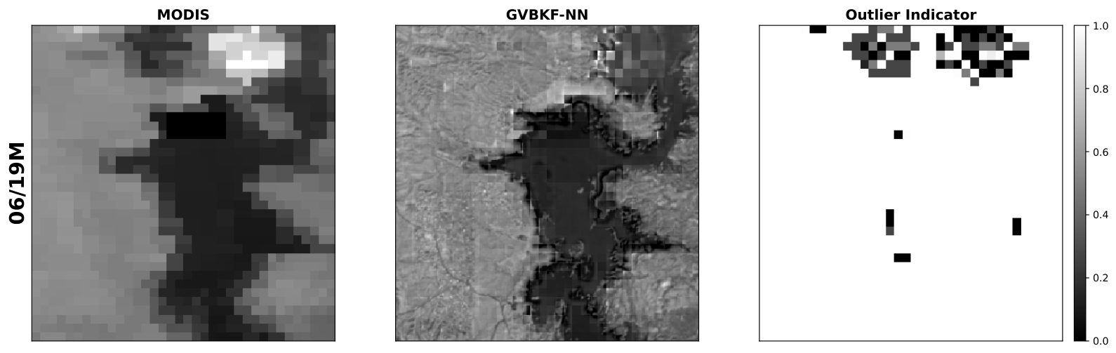
Figure A2 shows the histogram representing the probability of pixel values in the cloudy/cloudless case in different datasets. According to Figure A2, the distribution of the cloudy dataset for the Oroville Dam is far from that of the cloudless one, while the distribution of the cloudy dataset for the Elephant Butte site is almost the same as the cloudless one. Since the outlier model adopted in this work is based on the high magnitude of outlier pixels, this means that the outlier indicator is more likely to be 1 in the Elephant Butte dataset compared with the Oroville Dam dataset, leading to a larger in (15). According to (16), we should initialize hyperparameters as larger but smaller to achieve this goal. In summary, this shows that the hyperparameters of the robust variational image fusion framework have to be adjusted according to the difference in typical values of in-distribution and outlier pixels.
Figure A2.
Histogram showing the distribution of pixel values in the Oroville Dam (top panel) and Elephant Butte (lower panel) images. The blue bars represent pixel values in the cloudless case, while the red bars indicate pixel values in the cloudy case.
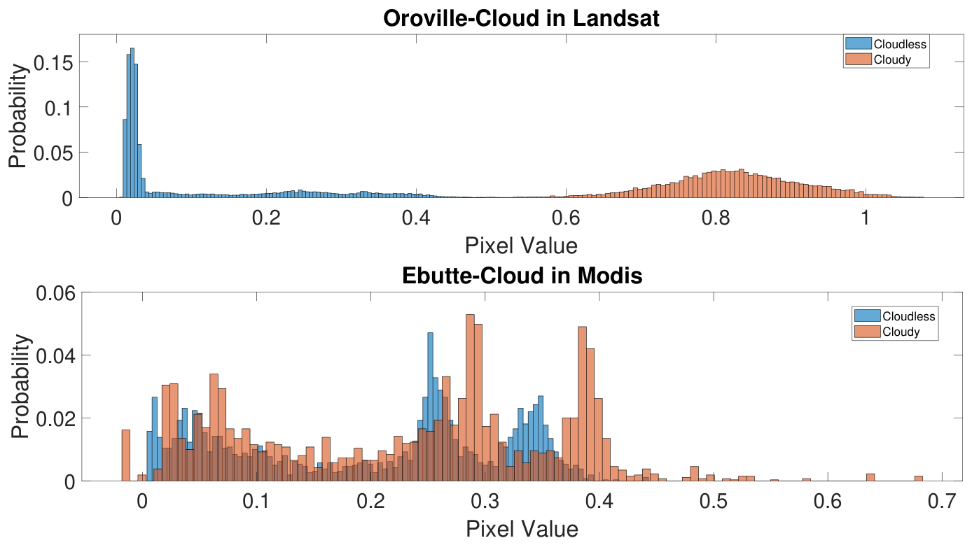
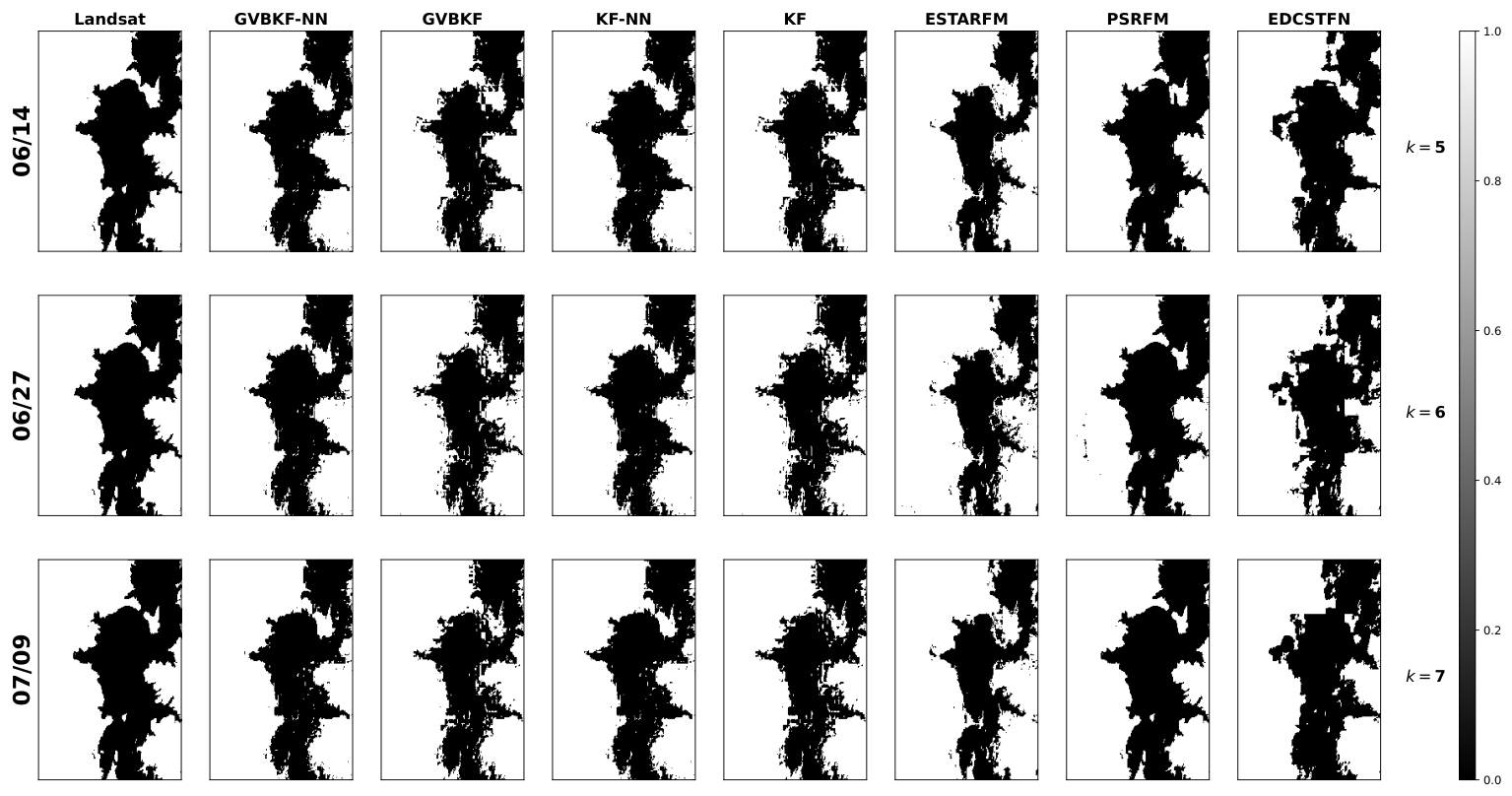
Figure A3 shows fused red reflectance as well as the acquired red-band reflectance values at MODIS and Landsat bands for the Elephant Butte site in the cloudless scenario. In the top labels, acquisition dates represent the acquired date. If the images are processed by the fusion algorithm, we have M for MODIS and L for Landsat, following the date in the top label. As shown in the figure, only the first and last Landsat images were used in the fusion process, while the remaining two images were used as ground truth to measure the performance of different methods. Figure A4 presents the water maps for the ground truth (first column) and all studied algorithms obtained using K-means clustering.
Figure A7 shows the fused red and NIR band results as well as the observations and ground truth in the Oroville Dam site in the cloudless scenario. In the top labels, acquisition dates represent the acquired date. If the images are processed by the fusion algorithm, we have M for MODIS and L for Landsat, following the date in the top label. As shown in the figure, only the first and last Landsat images were used in the fusion process, while the remaining two images were used as ground truth to measure the performance of different methods. We can see that the fused images by all different methods are similar to the Landsat (ground truth) images visually. The upper panel of Figure A8 presents the water maps for all different algorithms based on K-means clustering, with the ground truth shown in the first column, while the lower panel of Figure A8 shows the misclassification maps (i.e., the absolute error between the water maps produced by the studied algorithms and the ground truth). By comparing all the methods, we can see that their results are visually similar.
Figure A3.
Fusion results for the red band from MODIS (band 1) and Landsat (band 4) for the Elephant Butte example in the cloudless case. The first two rows show the observed images at MODIS and Landsat bands. At each time index, the fused images by GVBKF-NN, GVBKF, KF-NN, KF, ESTARFM, PSRFM and EDCSTFN are presented in the following rows. Note that some Landsat images were used solely as ground truth with only the acquisition date as the top label, while images processed by the algorithms are indicated by the top labels, where “M” stands for MODIS and “L” for Landsat.
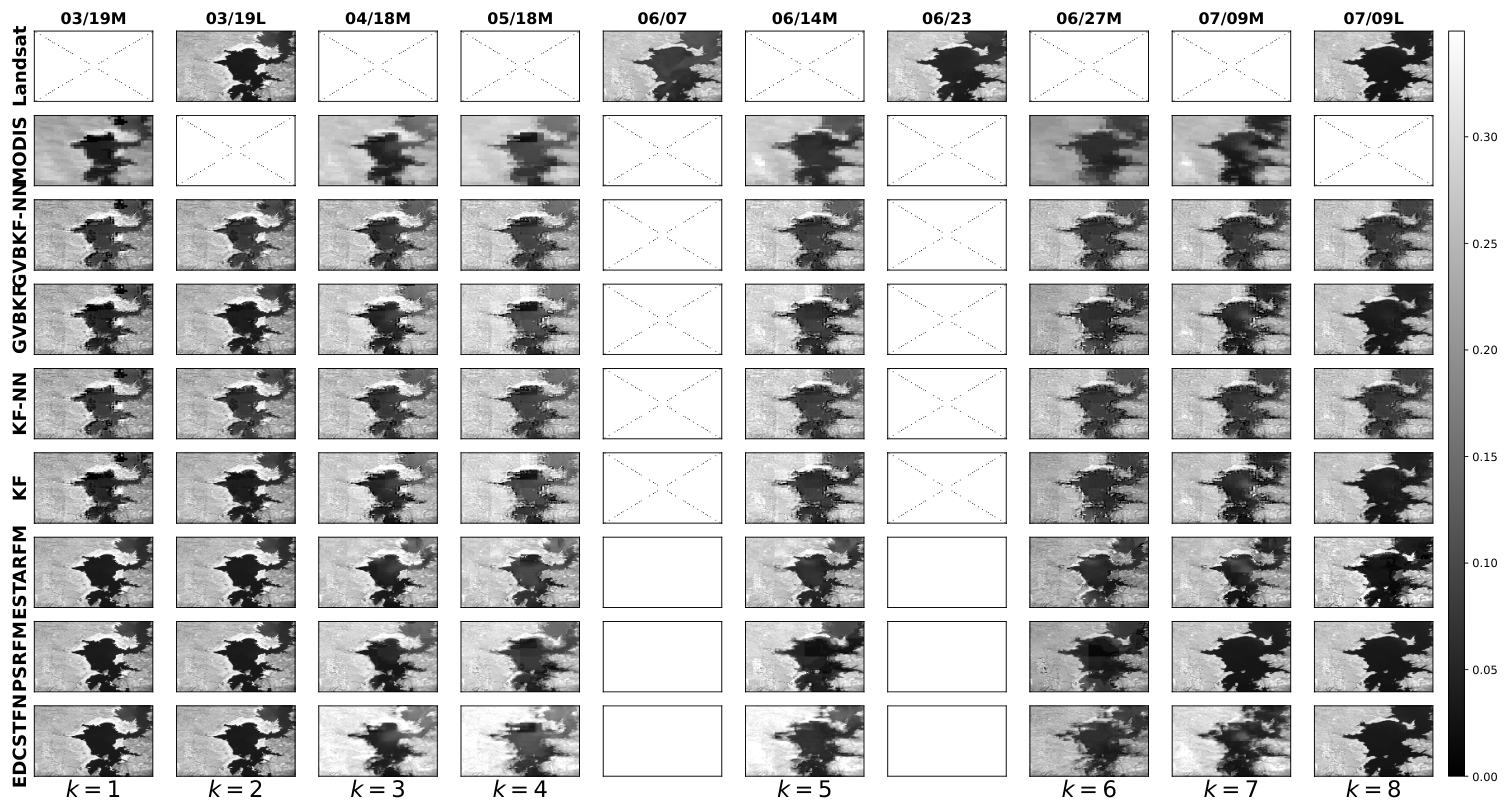
Figure A4.
Water map of the reconstructed images in the Elephant Butte cloudless case based on the K-means clustering strategy. In the plot, 1 represents land, and 0 is a water pixel. Classification maps obtained from Landsat images that are not processed by the algorithms act as the ground truth in the first column.
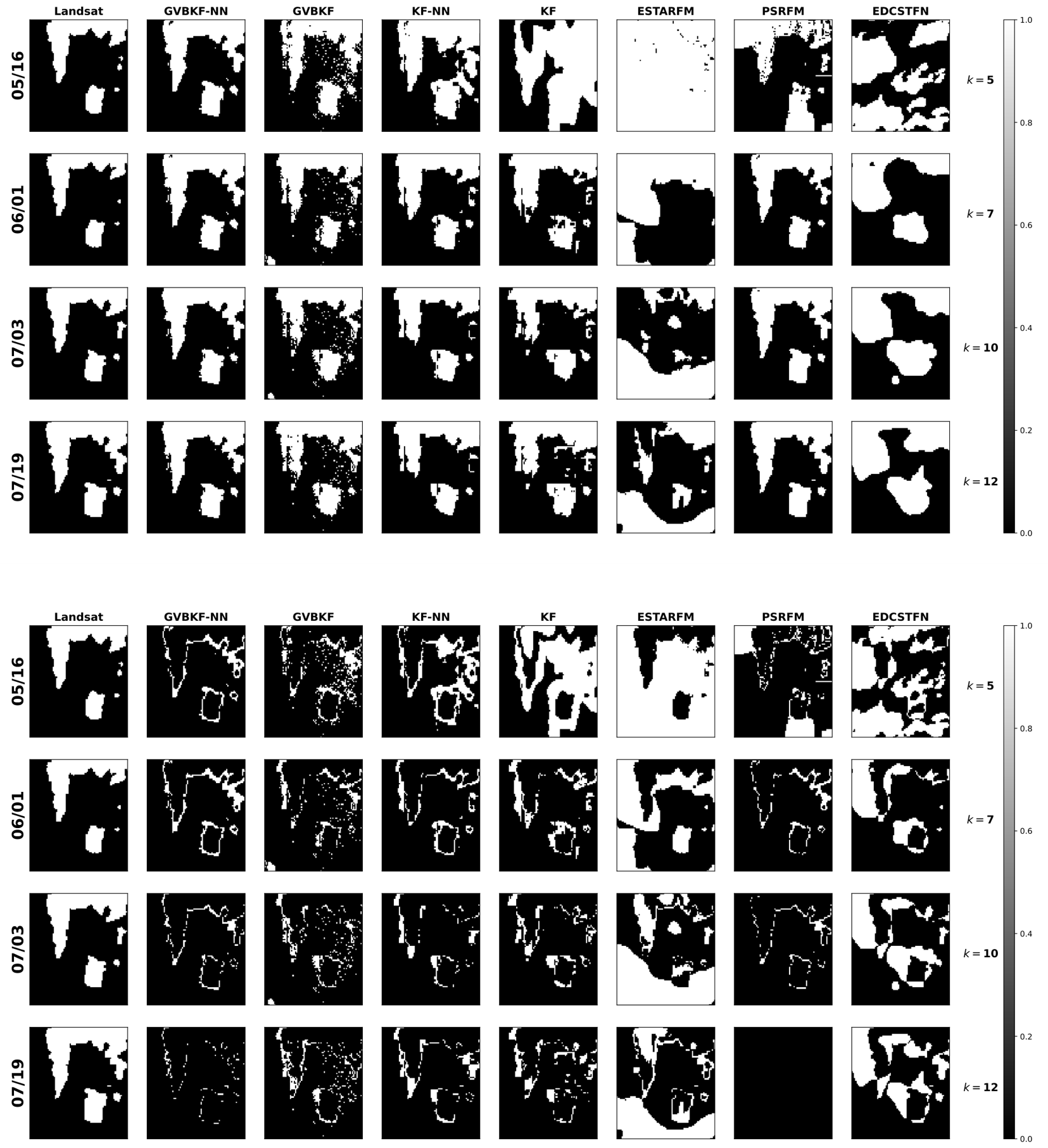
Similarly, Figure A9 shows the fused red reflectance results with the acquired images and ground truth for the Oroville Dam site in the cloudy scenario. The upper panel of Figure A10 presents the water maps for all different algorithms, with the ground truth shown in the first column, based on K-means clustering, while the lower panel of Figure A10 shows the misclassification maps (i.e., the absolute error between the water maps produced by the studied algorithms and the ground truth). Note that the ground truth for 16 May in Figure A10 was obtained by an interpolation method. We can see from the results that the images estimated by the KF, the ESTARFM, the EDCSTFN, and even the PSRFM are heavily influenced by the large cloud cover in the Landsat observation from 05/16. On the other hand, the GVBKF, KF-NN and GVBKF-NN methods exhibit relatively stable performance, keeping the estimated images robust against large cloud cover. This is also seen in the misclassification maps, where as shown in Figure A10, the KF, the ESTARFM, the EDCSTFN, and even the PSRFM present much larger error compared with the other three methods, among which the GVBKF-NN has the smallest number of misclassifications.
Figure A5.
Fusion results for the red band from MODIS (band 1) and Landsat (band 4) for the Elephant Butte example in the cloudy case. The first two rows show the observed images at MODIS and Landsat bands. At each time index, the fused images by GVBKF-NN, GVBKF, KF-NN, KF, ESTARFM, PSRFM and EDCSTFN are presented in the following rows. Note that some Landsat images were used solely as ground truth with only the acquisition date as the top label, while images processed by the algorithms are indicated by the top labels, where “M” stands for MODIS and “L” for Landsat.
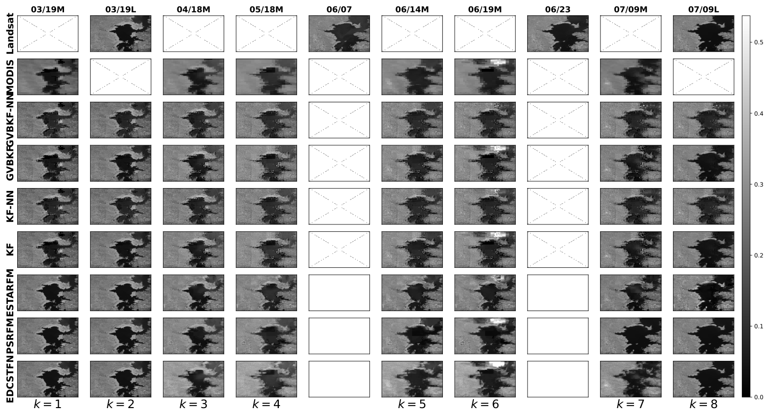
Figure A6.
Water map of the fused images in the Elephant Butte cloudy case based on the K-means clustering strategy. In the plot, 1 represents land, and 0 is a water pixel. Classification maps obtained from Landsat images that are not processed by the algorithms act as the ground truth in the first column.
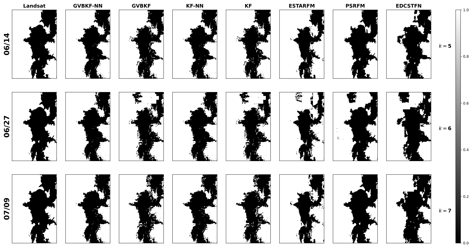
Figure A7.
Fused NIR and red bands from MODIS (upper subfigure for band 2 and lower subfigure for band 1) and Landsat (upper subfigure for band 5 and lower subfigure for band 4) for the Oroville Dam example in the cloudless case using different strategies. The first two rows of the top and bottom subfigures show the observed images at MODIS and Landsat bands. At each time index, the fused images given by GVBKF-NN, GVBKF, KF-NN, KF, ESTARFM, PSRFM and EDCSTFN are presented in the following rows. Note that some Landsat images were used solely as ground truth with only the acquisition date as the top label, while the images used are indicated by the top labels, where “M” stands for MODIS and “L” for Landsat.
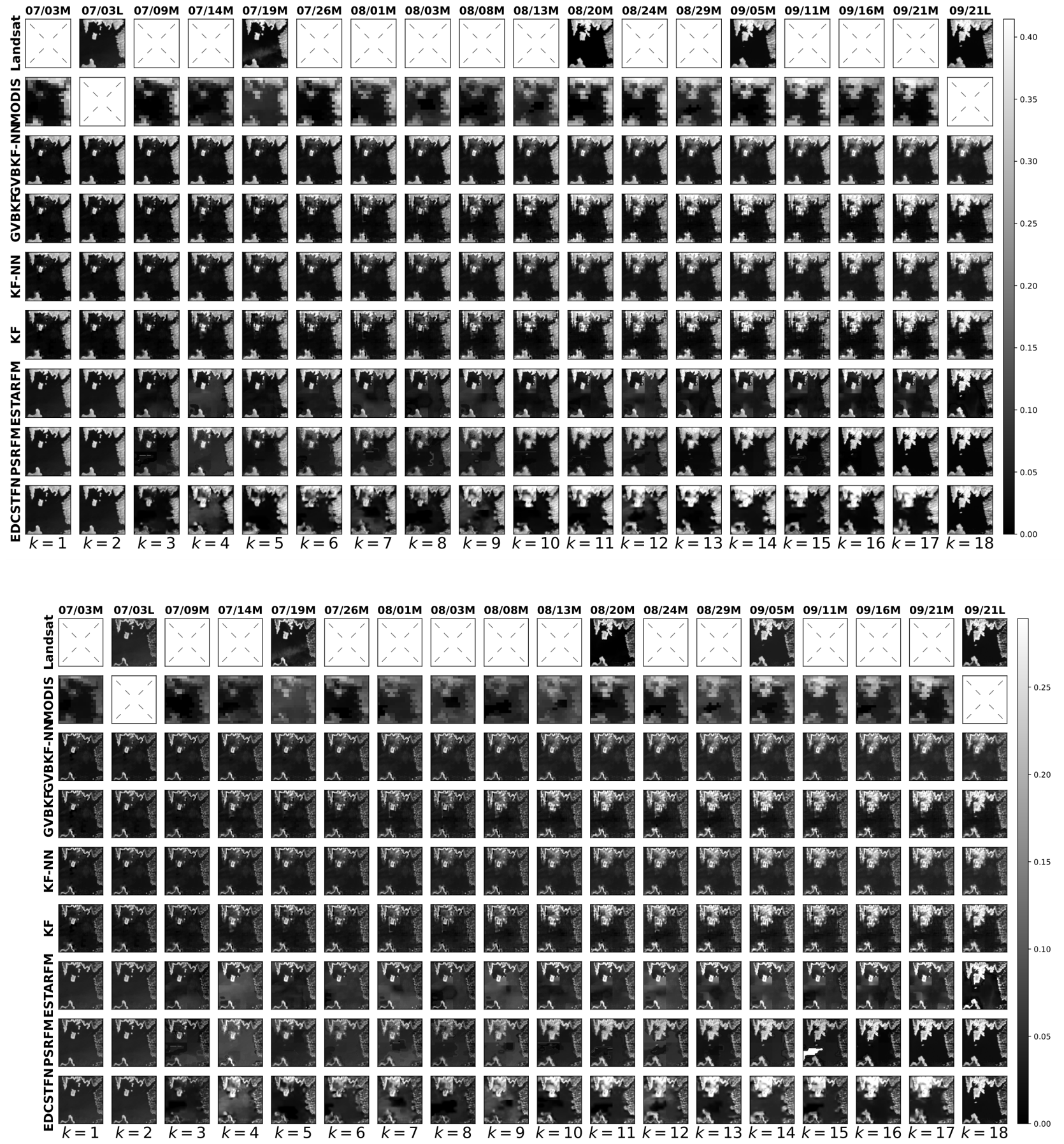
Figure A8.
(Upper Panel) Water map of the fused results in the Oroville Dam cloudless case based on the K-means clustering strategy. In the plot, 1 represents land, and 0 is a water pixel. Classification maps obtained from Landsat images that are not processed by the algorithms act as the ground truth in the first column. (Lower Panel) Absolute error of water map of images based on K-means clustering strategy. In this plot, a 0 pixel value indicates correct classification, and a 1 pixel value indicates misclassification. For comparison, the acquired Landsat images are shown in the first column as the ground truth.
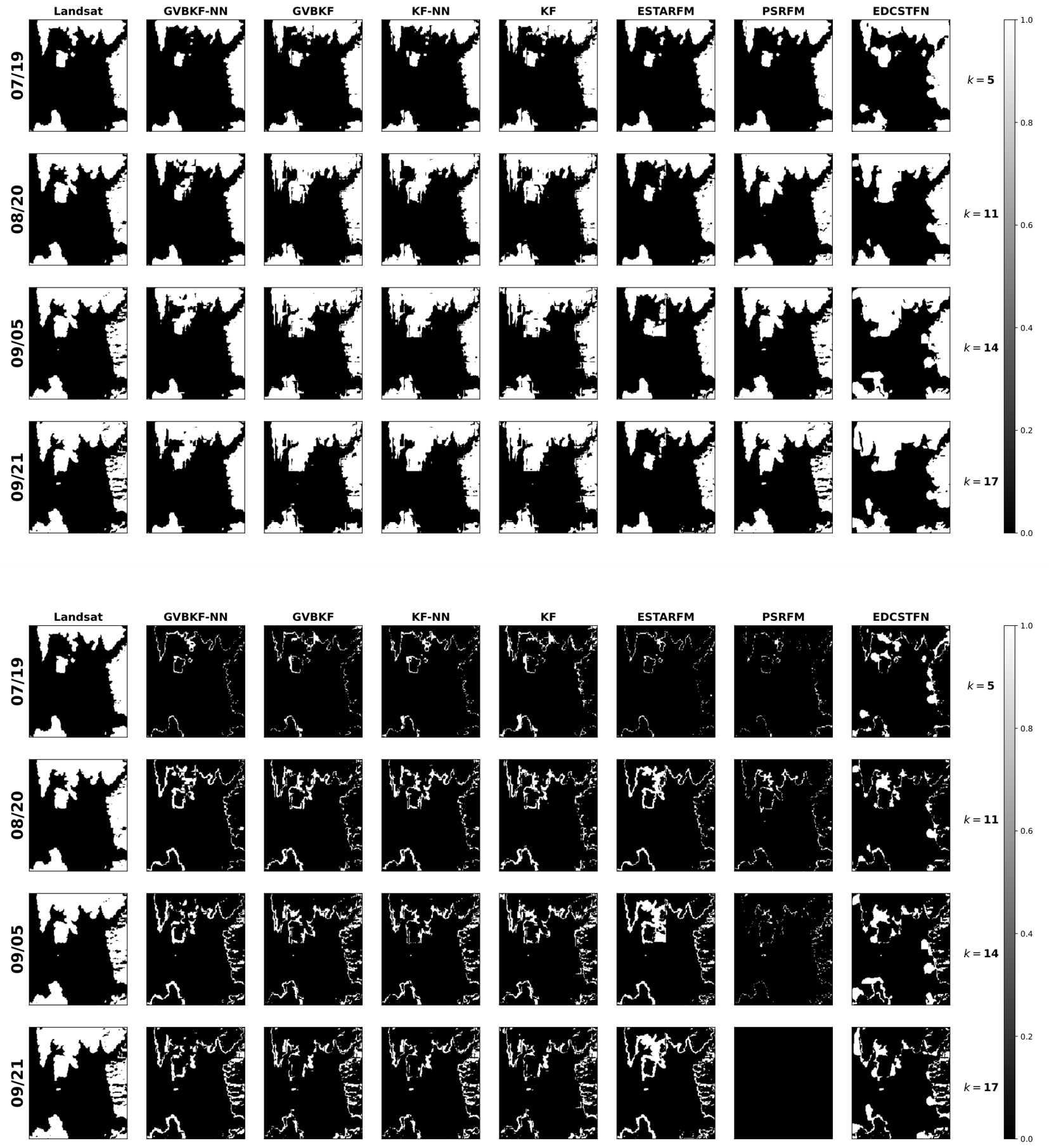
Figure A9.
Fused NIR and red bands from MODIS (upper subfigure for band 2 and lower subfigure for band 1) and Landsat (upper subfigure for band 5 and lower subfigure for band 4) for the Oroville Dam example in the cloudy case using different strategies. The first two rows of the top and bottom subfigures show the observed images at MODIS and Landsat bands. At each time index, the fused images by GVBKF-NN, GVBKF, KF-NN, KF, ESTARFM, PSRFM and EDCSTFN are presented in the following rows. Note that some Landsat images were used solely as ground truth with only the acquisition date as the top label, while images used are indicated by the top labels, where “M” stands for MODIS and “L” for Landsat.
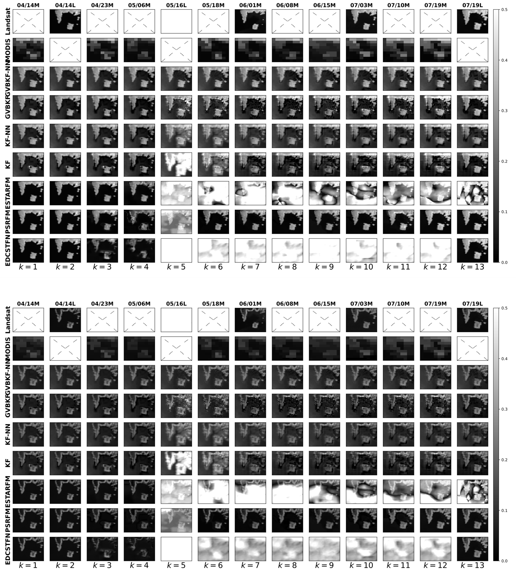
Figure A10.
(Upper Panel) Water map of the fused images in the Oroville Dam example in the cloudy case based on the K-means clustering strategy. In the plot, 1 represents land, and 0 is a water pixel. Classification maps obtained from Landsat images that are not processed by the algorithms act as the ground truth in the first column. (Lower Panel) Absolute error of water map of images based on K-means clustering strategy. In this plot, a 0 pixel value indicates correct classification, and a 1 pixel value indicates misclassification. For comparison, the acquired Landsat images are shown in the first column as the ground truth (the Landsat ground truth from 05/16 is a surrogate one obtained using an interpolation strategy).
References
- Lu, M.; Chen, J.; Tang, H.; Rao, Y.; Yang, P.; Wu, W. Land cover change detection by integrating object-based data blending model of Landsat and MODIS. Remote Sens. Environ. 2016, 184, 374–386. [Google Scholar] [CrossRef] [Scilit]
- Schultz, M.; Clevers, J.G.; Carter, S.; Verbesselt, J.; Avitabile, V.; Quang, H.V.; Herold, M. Performance of vegetation indices from Landsat time series in deforestation monitoring. Int. J. Appl. Earth Obs. Geoinf. 2016, 52, 318–327. [Google Scholar] [CrossRef] [Scilit]
- Gholizadeh, M.H.; Melesse, A.M.; Reddi, L. A comprehensive review on water quality parameters estimation using remote sensing techniques. Sensors 2016, 16, 1298. [Google Scholar] [CrossRef] [Scilit] [PubMed]
- Roy, D.P.; Wulder, M.A.; Loveland, T.R.; Woodcock, C.E.; Allen, R.G.; Anderson, M.C.; Helder, D.; Irons, J.R.; Johnson, D.M.; Kennedy, R.; et al. Landsat-8: Science and product vision for terrestrial global change research. Remote Sens. Environ. 2014, 145, 154–172. [Google Scholar] [CrossRef] [Scilit]
- Wang, Q.; Atkinson, P.M. Spatio-temporal fusion for daily Sentinel-2 images. Remote Sens. Environ. 2018, 204, 31–42. [Google Scholar] [CrossRef] [Scilit]
- Yang, Y.; Anderson, M.C.; Gao, F.; Wood, J.D.; Gu, L.; Hain, C. Studying drought-induced forest mortality using high spatiotemporal resolution evapotranspiration data from thermal satellite imaging. Remote Sens. Environ. 2021, 265, 112640. [Google Scholar] [CrossRef] [Scilit]
- Li, X.; Foody, G.M.; Boyd, D.S.; Ge, Y.; Zhang, Y.; Du, Y.; Ling, F. SFSDAF: An enhanced FSDAF that incorporates sub-pixel class fraction change information for spatio-temporal image fusion. Remote Sens. Environ. 2020, 237, 111537. [Google Scholar] [CrossRef] [Scilit]
- Borsoi, R.A.; Erdogmus, D.; Imbiriba, T. Learning Interpretable Deep Disentangled Neural Networks for Hyperspectral Unmixing. IEEE Trans. Comput. Imaging 2023, 9, 977–991. [Google Scholar] [CrossRef] [Scilit]
- Zhu, X.; Chen, J.; Gao, F.; Chen, X.; Masek, J.G. An enhanced spatial and temporal adaptive reflectance fusion model for complex heterogeneous regions. Remote Sens. Environ. 2010, 114, 2610–2623. [Google Scholar] [CrossRef] [Scilit]
- Xu, S.; Cheng, J. A new land surface temperature fusion strategy based on cumulative distribution function matching and multiresolution Kalman filtering. Remote Sens. Environ. 2021, 254, 112256. [Google Scholar] [CrossRef] [Scilit]
- Li, H.; Duvvuri, B.; Borsoi, R.; Imbiriba, T.; Beighley, E.; Erdoğmuş, D.; Closas, P. Online fusion of multi-resolution multispectral images with weakly supervised temporal dynamics. ISPRS J. Photogramm. Remote Sens. 2023, 196, 471–489. [Google Scholar] [CrossRef] [Scilit]
- Benzenati, T.; Kallel, A.; Kessentini, Y. STF-Trans: A two-stream spatiotemporal fusion transformer for very high resolution satellites images. Neurocomputing 2024, 563, 126868. [Google Scholar] [CrossRef] [Scilit]
- Zhu, C.; Song, X.; Li, Y.; Deng, S.; Zhang, T. A spatial-frequency dual-domain implicit guidance method for hyperspectral and multispectral remote sensing image fusion based on Kolmogorov-Arnold Network. Inf. Fusion 2025, 123, 103261. [Google Scholar] [CrossRef] [Scilit]
- Zhan, Y.; Xiong, Z.; Yuan, Y. Skyeyegpt: Unifying remote sensing vision-language tasks via instruction tuning with large language model. ISPRS J. Photogramm. Remote Sens. 2025, 221, 64–77. [Google Scholar] [CrossRef] [Scilit]
- Ma, J.; Tang, L.; Xu, M.; Zhang, H.; Xiao, G. STDFusionNet: An infrared and visible image fusion network based on salient target detection. IEEE Trans. Instrum. Meas. 2021, 70, 5009513. [Google Scholar] [CrossRef] [Scilit]
- Wang, Z.; Zhou, D.; Li, X.; Zhu, L.; Gong, H.; Ke, Y. Virtual image-based cloud removal for Landsat images. GIScience Remote Sens. 2023, 60, 2160411. [Google Scholar] [CrossRef] [Scilit]
- Siravenha, A.C.; Sousa, D.; Bispo, A.; Pelaes, E. Evaluating inpainting methods to the satellite images clouds and shadows removing. In Proceedings of the Signal Processing, Image Processing and Pattern Recognition: International Conference, Jeju Island, Korea, 8–10 December 2011; Springer: Berlin/Heidelberg, Germany, 2011; pp. 56–65. [Google Scholar]
- Xu, M.; Deng, F.; Jia, S.; Jia, X.; Plaza, A.J. Attention mechanism-based generative adversarial networks for cloud removal in Landsat images. Remote Sens. Environ. 2022, 271, 112902. [Google Scholar] [CrossRef] [Scilit]
- Meraner, A.; Ebel, P.; Zhu, X.X.; Schmitt, M. Cloud removal in Sentinel-2 imagery using a deep residual neural network and SAR-optical data fusion. ISPRS J. Photogramm. Remote Sens. 2020, 166, 333–346. [Google Scholar] [CrossRef] [Scilit] [PubMed]
- Shen, H.; Wu, J.; Cheng, Q.; Aihemaiti, M.; Zhang, C.; Li, Z. A spatiotemporal fusion based cloud removal method for remote sensing images with land cover changes. IEEE J. Sel. Top. Appl. Earth Obs. Remote Sens. 2019, 12, 862–874. [Google Scholar] [CrossRef] [Scilit]
- Zhang, Q.; Yuan, Q.; Li, J.; Li, Z.; Shen, H.; Zhang, L. Thick cloud and cloud shadow removal in multitemporal imagery using progressively spatio-temporal patch group deep learning. ISPRS J. Photogramm. Remote Sens. 2020, 162, 148–160. [Google Scholar] [CrossRef] [Scilit]
- Tan, Z.; Gao, M.; Yuan, J.; Jiang, L.; Duan, H. A Robust Model for MODIS and Landsat Image Fusion Considering Input Noise. IEEE Trans. Geosci. Remote Sens. 2022, 60, 5407217. [Google Scholar] [CrossRef] [Scilit]
- Särkkä, S. Bayesian Filtering and Smoothing; Number 3; Cambridge University Press: Cambridge, UK, 2013. [Google Scholar]
- Sedano, F.; Kempeneers, P.; Hurtt, G. A Kalman filter-based method to generate continuous time series of medium-resolution NDVI images. Remote Sens. 2014, 6, 12381–12408. [Google Scholar] [CrossRef] [Scilit]
- Zhou, F.; Zhong, D. Kalman filter method for generating time-series synthetic Landsat images and their uncertainty from Landsat and MODIS observations. Remote Sens. Environ. 2020, 239, 111628. [Google Scholar] [CrossRef] [Scilit]
- Gao, Z.; Tan, C.; Wu, L.; Li, S.Z. SimVP: Simpler yet better video prediction. In Proceedings of the IEEE/CVF Conference on Computer Vision and Pattern Recognition, New Orleans, LA, USA, 18–24 June 2022; pp. 3170–3180. [Google Scholar]
- Voleti, V.; Jolicoeur-Martineau, A.; Pal, C. MCVD-masked conditional video diffusion for prediction, generation, and interpolation. Proc. Adv. Neural Inf. Process. Syst. 2022, 35, 23371–23385. [Google Scholar]
- Li, H.; Medina, D.; Vilà-Valls, J.; Closas, P. Robust variational-based Kalman filter for outlier rejection with correlated measurements. IEEE Trans. Signal Process. 2020, 69, 357–369. [Google Scholar] [CrossRef] [Scilit]
- Li, W.; Yang, C.; Peng, Y.; Du, J. A pseudo-siamese deep convolutional neural network for spatiotemporal satellite image fusion. IEEE J. Sel. Top. Appl. Earth Obs. Remote Sens. 2022, 15, 1205–1220. [Google Scholar] [CrossRef] [Scilit]
- Chen, Y.; Shi, K.; Ge, Y.; Zhou, Y. Spatiotemporal remote sensing image fusion using multiscale two-stream convolutional neural networks. IEEE Trans. Geosci. Remote Sens. 2021, 60, 4402112. [Google Scholar] [CrossRef] [Scilit]
- Zhou, G.; Tian, C.; Niu, C.; Jing, G.; Miao, H.; Li, Z. Short time cloud-free image reconstruction based on time series images. IEEE J. Sel. Top. Appl. Earth Obs. Remote Sens. 2023, 16, 51–65. [Google Scholar] [CrossRef] [Scilit]
- Li, H.; Borsoi, R.; Imbiriba, T.; Closas, P. A Variational Approach for Robust Online Fusion of Multiresolution Multispectral Images. In Proceedings of the 2024 32nd European Signal Processing Conference (EUSIPCO), Lyon, France, 26–30 August 2024; IEEE: Piscataway, NJ, USA, 2024; pp. 666–670. [Google Scholar]
- Borsoi, R.A.; Costa, G.H.; Bermudez, J.C.M. A new adaptive video super-resolution algorithm with improved robustness to innovations. IEEE Trans. Image Process. 2018, 28, 673–686. [Google Scholar] [CrossRef] [Scilit]
- Oprea, S.; Martinez-Gonzalez, P.; Garcia-Garcia, A.; Castro-Vargas, J.A.; Orts-Escolano, S.; Garcia-Rodriguez, J.; Argyros, A. A review on deep learning techniques for video prediction. IEEE Trans. Pattern Anal. Mach. Intell. 2020, 44, 2806–2826. [Google Scholar] [CrossRef] [Scilit]
- Wang, Y.; Wu, H.; Zhang, J.; Gao, Z.; Wang, J.; Philip, S.Y.; Long, M. PredRNN: A recurrent neural network for spatiotemporal predictive learning. IEEE Trans. Pattern Anal. Mach. Intell. 2022, 45, 2208–2225. [Google Scholar] [CrossRef] [Scilit]
- Rakhimov, R.; Volkhonskiy, D.; Artemov, A.; Zorin, D.; Burnaev, E. Latent video transformer. arXiv 2020, arXiv:2006.10704. [Google Scholar] [CrossRef] [Scilit]
- Franceschi, J.Y.; Delasalles, E.; Chen, M.; Lamprier, S.; Gallinari, P. Stochastic latent residual video prediction. In Proceedings of the International Conference on Machine Learning, Virtual, 13–18 July 2020; PMLR: London, UK, 2020; pp. 3233–3246. [Google Scholar]
- Borsoi, R.A.; Imbiriba, T.; Closas, P. Dynamical Hyperspectral Unmixing with Variational Recurrent Neural Networks. IEEE Trans. Image Process. 2023, 32, 2279–2294. [Google Scholar] [CrossRef] [Scilit]
- Blattmann, A.; Rombach, R.; Ling, H.; Dockhorn, T.; Kim, S.W.; Fidler, S.; Kreis, K. Align your latents: High-resolution video synthesis with latent diffusion models. In Proceedings of the IEEE/CVF Conference on Computer Vision and Pattern Recognition, Vancouver, BC, Canada, 17–24 June 2023; pp. 22563–22575. [Google Scholar]
- Singh, A.; Borsoi, R.A.; Erdogmus, D.; Imbiriba, T. Learning semilinear neural operators: A unified recursive framework for prediction and data assimilation. In Proceedings of the the Twelfth International Conference on Learning Representations (ICLR), Vienna, Austria, 7–11 May 2024. [Google Scholar]
- Jiao, L.; Zhang, X.; Liu, X.; Liu, F.; Yang, S.; Ma, W.; Li, L.; Chen, P.; Feng, Z.; Guo, Y.; et al. Transformer Meets Remote Sensing Video Detection and Tracking: A Comprehensive Survey. IEEE J. Sel. Top. Appl. Earth Obs. Remote Sens. 2023, 16, 1–45. [Google Scholar] [CrossRef] [Scilit]
- Oh, J.; Guo, X.; Lee, H.; Lewis, R.L.; Singh, S. Action-conditional video prediction using deep networks in Atari games. In Proceedings of the Advances in Neural Information Processing Systems, Montreal, QC, Canada, 7–12 December 2015; Volume 28. [Google Scholar]
- Finn, C.; Goodfellow, I.; Levine, S. Unsupervised learning for physical interaction through video prediction. In Proceedings of the Advances in Neural Information Processing Systems, Barcelona, Spain, 5–10 December 2016; Volume 29. [Google Scholar]
- Li, X.; Peng, Q.; Zheng, Y.; Lin, S.; He, B.; Qiu, Y.; Chen, J.; Chen, Y.; Yuan, W. Incorporating environmental variables into spatiotemporal fusion model to reconstruct high-quality vegetation index data. IEEE Trans. Geosci. Remote Sens. 2024, 62, 4401812. [Google Scholar] [CrossRef] [Scilit]
- Arasaratnam, I.; Haykin, S. Cubature Kalman Filters. IEEE Trans. Autom. Control 2009, 54, 1254–1269. [Google Scholar] [CrossRef] [Scilit]
- Closas, P.; Fernandez-Prades, C.; Vila-Valls, J. Multiple quadrature Kalman filtering. IEEE Trans. Signal Process. 2012, 60, 6125–6137. [Google Scholar] [CrossRef] [Scilit]
- Vilà-Valls, J.; Closas, P.; García-Fernández, Á.F. Uncertainty exchange through multiple quadrature Kalman filtering. IEEE Signal Process. Lett. 2016, 23, 1825–1829. [Google Scholar] [CrossRef] [Scilit]
- Vilà-Valls, J.; Closas, P.; García-Fernández, Á.F.; Fernández-Prades, C. Multiple sigma-point Kalman smoothers for high-dimensional state-space models. In Proceedings of the 2017 IEEE 7th International Workshop on Computational Advances in Multi-Sensor Adaptive Processing (CAMSAP), Curacao, Dutch Antilles, 10–13 December 2017; IEEE: Piscataway, NJ, USA, 2017; pp. 1–5. [Google Scholar]
- Gao, B.C. NDWI–A normalized difference water index for remote sensing of vegetation liquid water from space. Remote Sens. Environ. 1996, 58, 257–266. [Google Scholar] [CrossRef] [Scilit]
- Huang, B.; Zhang, H.; Song, H.; Wang, J.; Song, C. Unified fusion of remote-sensing imagery: Generating simultaneously high-resolution synthetic spatial–temporal–spectral earth observations. Remote Sens. Lett. 2013, 4, 561–569. [Google Scholar] [CrossRef] [Scilit]
- Zhong, D.; Zhou, F. A prediction smooth method for blending landsat and moderate resolution imagine spectroradiometer images. Remote Sens. 2018, 10, 1371. [Google Scholar] [CrossRef] [Scilit]
- Tan, Z.; Di, L.; Zhang, M.; Guo, L.; Gao, M. An enhanced deep convolutional model for spatiotemporal image fusion. Remote Sens. 2019, 11, 2898. [Google Scholar] [CrossRef] [Scilit]
- Singh, S.; Singh, H.; Bueno, G.; Deniz, O.; Singh, S.; Monga, H.; Hrisheekesha, P.; Pedraza, A. A review of image fusion: Methods, applications and performance metrics. Digit. Signal Process. 2023, 137, 104020. [Google Scholar] [CrossRef] [Scilit]
- Lv, M.; Song, S.; Jia, Z.; Li, L.; Ma, H. Multi-focus image fusion based on dual-channel Rybak neural network and consistency verification in NSCT domain. Fractal Fract. 2025, 9, 432. [Google Scholar] [CrossRef] [Scilit]
- Saroglu, E.; Bektas, F.; Musaoglu, N.; Goksel, C. Fusion of multisensor remote sensing data: Assessing the quality of resulting images. Int. Arch. Photogram. Rem. Sens. Spatial. Inform. Sci. 2004, 35, 575–579. [Google Scholar]
- Roberts, J.W.; Van Aardt, J.A.; Ahmed, F.B. Assessment of image fusion procedures using entropy, image quality, and multispectral classification. J. Appl. Remote Sens. 2008, 2, 023522. [Google Scholar]
- Saibaba, A.K.; Miller, E.L.; Kitanidis, P.K. Fast Kalman filter using hierarchical matrices and a low-rank perturbative approach. Inverse Probl. 2015, 31, 015009. [Google Scholar] [CrossRef] [Scilit]
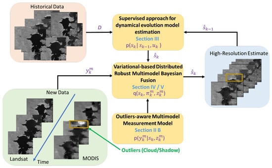
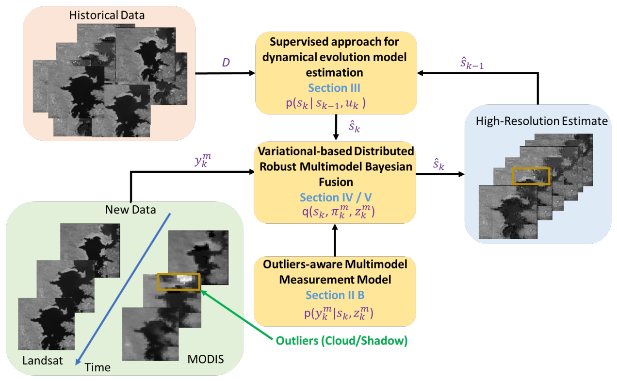
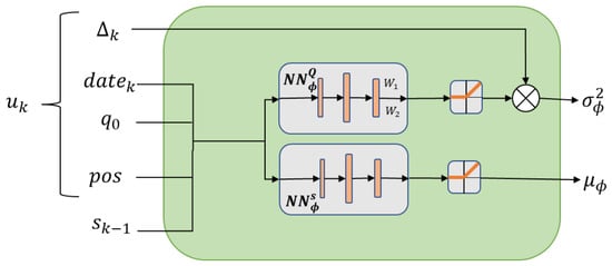
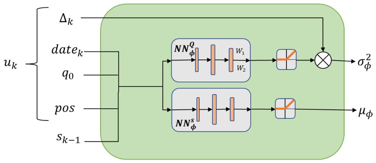
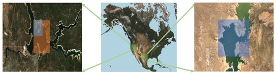
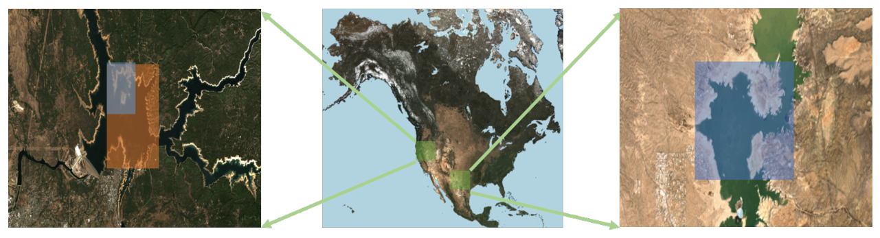
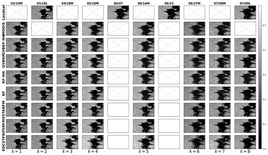
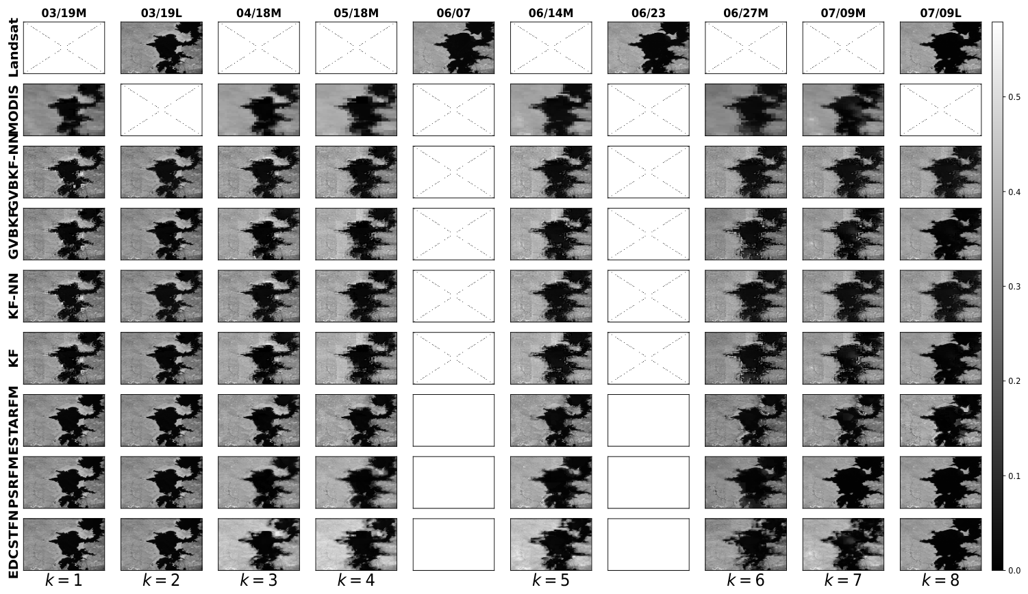
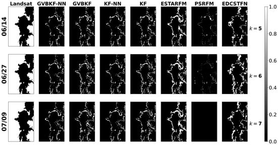
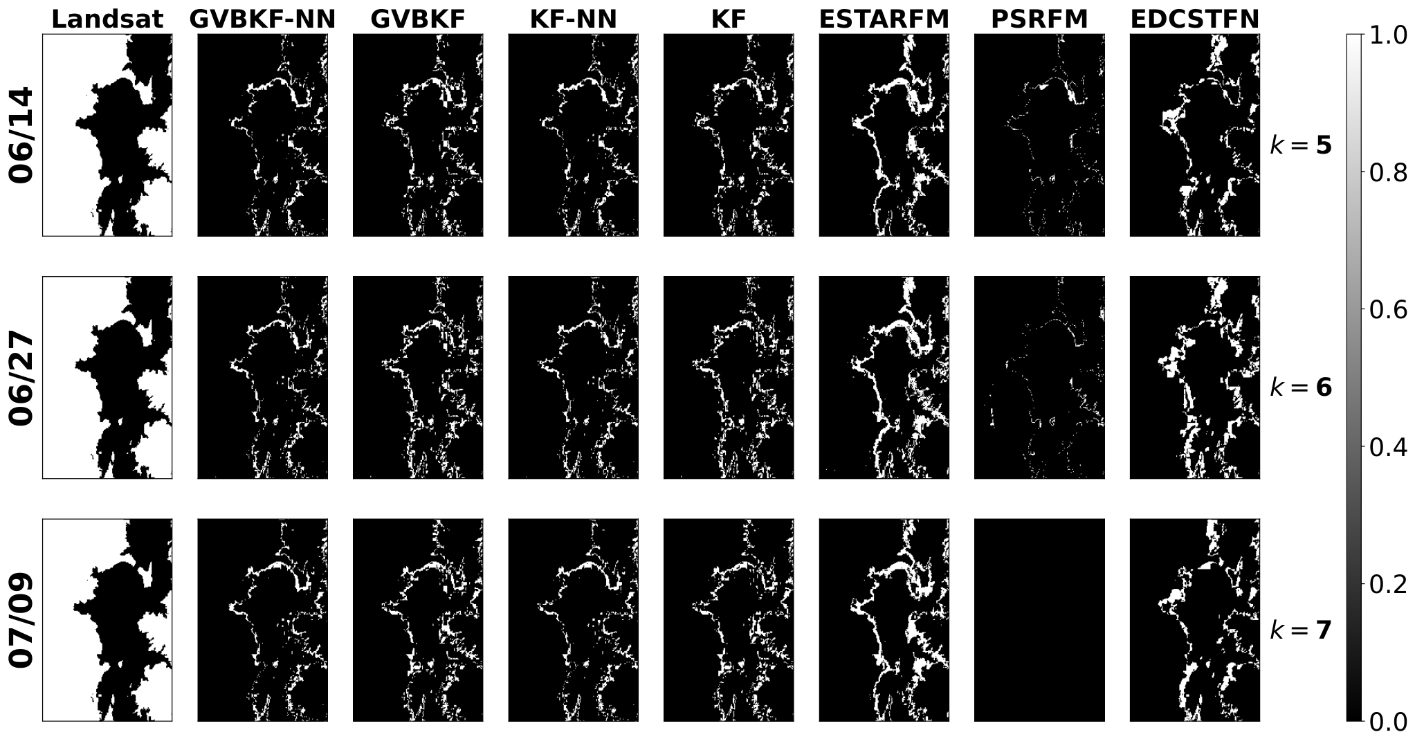
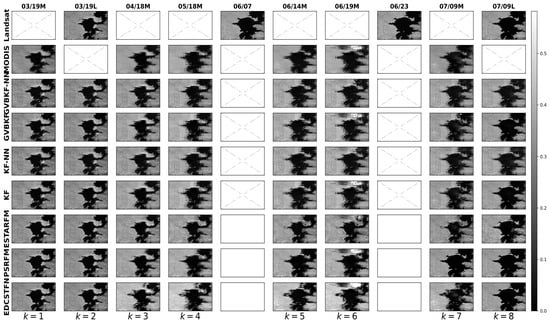
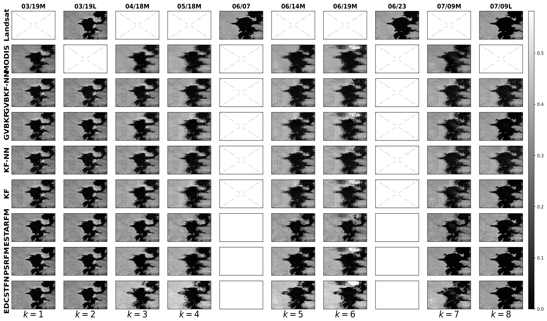
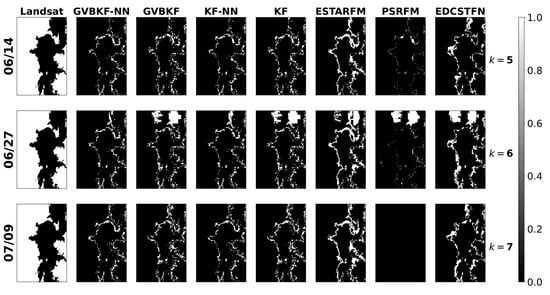
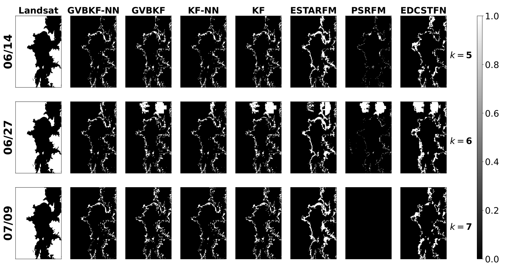

Disclaimer/Publisher’s Note: The statements, opinions and data contained in all publications are solely those of the individual author(s) and contributor(s) and not of MDPI and/or the editor(s). MDPI and/or the editor(s) disclaim responsibility for any injury to people or property resulting from any ideas, methods, instructions or products referred to in the content. |
© 2026 by the authors. Licensee MDPI, Basel, Switzerland. This article is an open access article distributed under the terms and conditions of the Creative Commons Attribution (CC BY) license.