


Highlights
What are the main findings?
- An exploratory top-down framework was established using TROPOMI and a differential evolution algorithm, exhibiting consistent city-scale emission estimation performance ().
- Spatial heterogeneity was identified across Shandong Province, with Jinan, Linyi, and Qingdao identified as the primary anthropogenic hotspots within this seasonal window.
What are the implications of the main findings?
- The implementation of the – relationship as a proxy provides a complementary, high-frequency technical perspective for carbon accounting in complex urban environments.
- The refined city-scale emission maps offer useful data support for characterizing localized emission patterns and evaluating regional carbon mitigation strategies.
Abstract
Since the Industrial Revolution, anthropogenic activities, primarily fossil fuel combustion, have driven a sharp increase in emissions, making them the principal driver of global climate change. Precise monitoring and quantification of emissions are essential for effective greenhouse gas mitigation. Traditional “bottom-up” inventories often suffer from limited timeliness, low spatial resolution, and significant uncertainties. Satellite remote sensing offers an alternative “top-down” approach for emission estimation. Compared to existing sensors, observation satellites provide higher spatiotemporal resolution. Given that and are co-emitted during combustion with a stable relationship, can serve as an effective proxy to indirectly derive emissions. In this study, an exploratory framework for city-scale estimation was developed using TROPOMI column concentrations, MERRA-2 wind fields, EDGAR inventory and the ODIAC inventory. The analysis focused on seven major cities in Shandong Province, China, from April to September 2022. By integrating a wind-rotation technique with a line density model and the differential evolution (DE) algorithm, we derived emissions and atmospheric lifetimes. The relationship was established based on sector-weighted inventory data to quantify fossil-fuel fluxes. The results identify Qingdao, Jinan, and Linyi as emission hotspots, followed by Rizhao, with lower emissions observed in Yantai, Liaocheng, and Jining. Comparison with the ODIAC inventory illustrates that this framework provides a top-down constraint for identifying localized emission characteristics and potential discrepancies in bottom-up datasets. This study offers a complementary tool for near-real-time urban carbon monitoring during the non-heating season.
1. Introduction
Since the Industrial Revolution, human activities, especially the burning of fossil fuels and land-use change, have emitted huge amounts of into the atmosphere. As is a major greenhouse gas, the sharp increase in its concentration is the core factor driving global climate change, which is directly related to a series of severe environmental challenges such as rising global average temperature, rising sea level, and frequent extreme climate events. According to the latest data from the Global Carbon Project, despite global efforts to combat climate change, global energy-related emissions reached a record 36.8 billion tonnes in 2022, only slightly down from their all-time high, and emissions levels are still at record highs overall [1].
The sixth assessment report released by the United Nations Intergovernmental Panel on Climate Change (IPCC) in 2023 once again emphasized that controlling carbon dioxide emissions is a necessary option to mitigate global warming [2]. Major countries around the world signed the Paris Agreement at the 2016 United Nations Climate Change Conference, which stipulates their emission reduction obligations. In 2020, China pledged to the international community to reach peak carbon emissions by 2030 and carbon neutrality by 2060. Carbon monitoring is a necessary means to quantify carbon emissions, and only through effective carbon monitoring can carbon emission data be obtained and the carbon mitigation policies and strategies can be formulated.
The use of fossil fuels related to urban power generation, heating, production, and transportation generates a large amount of greenhouse gas emissions, so cities contribute 70% of the world’s anthropogenic emissions as a major carbon source [3]. According to the 2018 World Urbanization Outlook report, the global population living in cities is expected to increase from 55% in 2018 to 68% in 2050. Cities are area sources of anthropogenic emissions, which lead to a corresponding increase in anthropogenic emissions of carbon dioxide. Therefore, monitoring and evaluating urban carbon emissions is a key basis for us understanding of carbon sources and planning carbon emission reduction measures.
However, traditional emission inventory methods, which are primarily based on “bottom-up” statistical models and rely on reported data on activities such as energy consumption, industrial production processes, etc., have significant limitations. This approach often has lags in reporting (often one to two years), a coarse spatial resolution (usually at the national or provincial level), and uncertainty due to differences in statistical capacity and transparency across countries [4].
In this context, satellite remote sensing technology, as a ’top-down’ observation method, has shown significant potential for independent emission verification. In recent years, with the launch of a series of hyperspectral greenhouse gas observation satellites (such as Japan’s GOSAT and GOSAT-2, the United States’ OCO-2 and OCO-3, and China’s TanSat, Fengyun-3D and Gaofen-5), satellite remote sensing has been able to measure column concentrations with high precision directly from space [5].
Recent studies have increasingly utilized high-resolution satellite data, such as TROPOMI, to quantify urban emissions. For instance, Liu et al. [6] developed a coupled method to map emissions at a resolution across 39 US cities, demonstrating the potential of satellite retrievals to bridge gaps in bottom-up inventories. High-resolution top-down emission inventories have exhibited substantial capabilities in identifying intense area sources such as cities and industrial clusters [7].
To improve the reliability of urban emission quantification, several recent studies have integrated wind rotation techniques with Gaussian fitting functions. For instance, Pommier [8] utilized TROPOMI observations to estimate emissions and lifetimes over three major British urban areas, demonstrating how wind-aligned plume analysis can refine discrepancies between satellite-derived data and bottom-up inventories.
The rotation technique prevents the neutralization of outflow patterns from opposite wind directions [9]. This allows the measurement points to be redistributed along the upwind–downwind direction for simultaneous analysis. Luo et al. [10] developed the SAT-SHIP model, which utilizes TROPOMI observations and varying wind patterns to successfully estimate shipping emissions for 17 major ports in China, demonstrating the feasibility of this approach in handling irregular emission plume signals.
While the use of satellite-derived as a proxy for has been explored in previous studies, achieving stable and localized urban-scale inversions in complex industrial regions like Shandong remains a challenge. The primary contribution of this work lies in the integrated synergy between the differential evolution (DE) algorithm and the line density framework. Unlike traditional local optimization methods that are sensitive to initial conditions, our framework leverages the global search capability of DE to simultaneously optimize multiple spatial parameters. This provides an additional top-down perspective to evaluate the spatial plausibility of the discrepancies found between bottom-up inventories like EDGAR and ODIAC [11].
Compared with —which primarily originates from surface combustion and has a shorter lifetime—estimating emissions using satellite remote sensing is significantly more difficult. This is mainly due to the unique physical and atmospheric properties of . is homogeneously mixed in the atmosphere, and its high background concentration (about 420 ppm) makes it extremely difficult to detect and separate anthropogenic emission signals, which account for only a very small portion of it (typically <1%), leading to greater estimation uncertainty [12].
and have a closely associated relationship in emissions. They are mainly derived from the oxidation reaction of fossil fuels (coal, oil, natural gas) during high-temperature combustion. Although there are differences in emission ratios caused by different fuel types, combustion technologies, and pollution control measures, this rate tends to remain relatively stable within a certain range for specific emission source categories and shorter time scales [13]. Therefore, theoretically, if emissions from satellites can be quantified with high reliability, and the emission ratio of a particular source is known or can be estimated, it is possible to indirectly estimate the emissions of the corresponding source. The advantage of this approach is that satellite sensors that observe (e.g., OMI, TROPOMI) have a longer observation history, higher spatiotemporal resolution (TROPOMI up to ), and higher spatial cover. This allows us to monitor carbon emissions at a finer scale and at a faster frequency [14,15].
At present, the research on estimating emissions using satellite observations has evolved from proof-of-concept studies toward more integrated implementations, showing considerable promise for emission monitoring. Early studies focused on establishing statistical relationships between and concentrations at the regional scale. For example, Reuter et al. [16] analyzed the column concentration correlation between two gases over several urban agglomerations and large point sources around the world using the data of OCO-2 and the data of TROPOMI, and supported the plausibility of using as a proxy index for tracking the spatial distribution of produced by fossil fuel combustion.
With advancements in emission inventory inversion technology, the focus of research has shifted to the direct use of emissions to constrain emissions. Zhang et al. [17] estimated Wuhan’s emissions by combining TROPOMI’s emissions with the preset ratio in the emissions inventory database, and the results exhibited good consistency with the bottom-up inventory data.
Significant progress has been made in research on the point sources, especially coal-fired power plants. Liu et al. [18] developed an algorithm based on the Gaussian diffusion model, using high-resolution TROPOMI data to successfully quantify the emission rates of many large coal-fired power plants in the United States, Europe and China. Recently, Schooling et al. [19] developed a data assimilation framework using TROPOMI to infer European fossil fuel emissions, highlighting the growing potential of using short-lived trace gases to isolate anthropogenic signals from biogenic .
In this study, we plan to use the TROPOMI’s column concentration data to match MERRA-2 wind field data, and utilize the rotational wind direction method to construct the line density distribution of tropospheric column concentrations to estimate surface emissions. Then and emission inventory are used to estimate the emission ratio of and in the cities in the study area, and finally the emissions of the target cities are obtained.
2. Materials and Methods
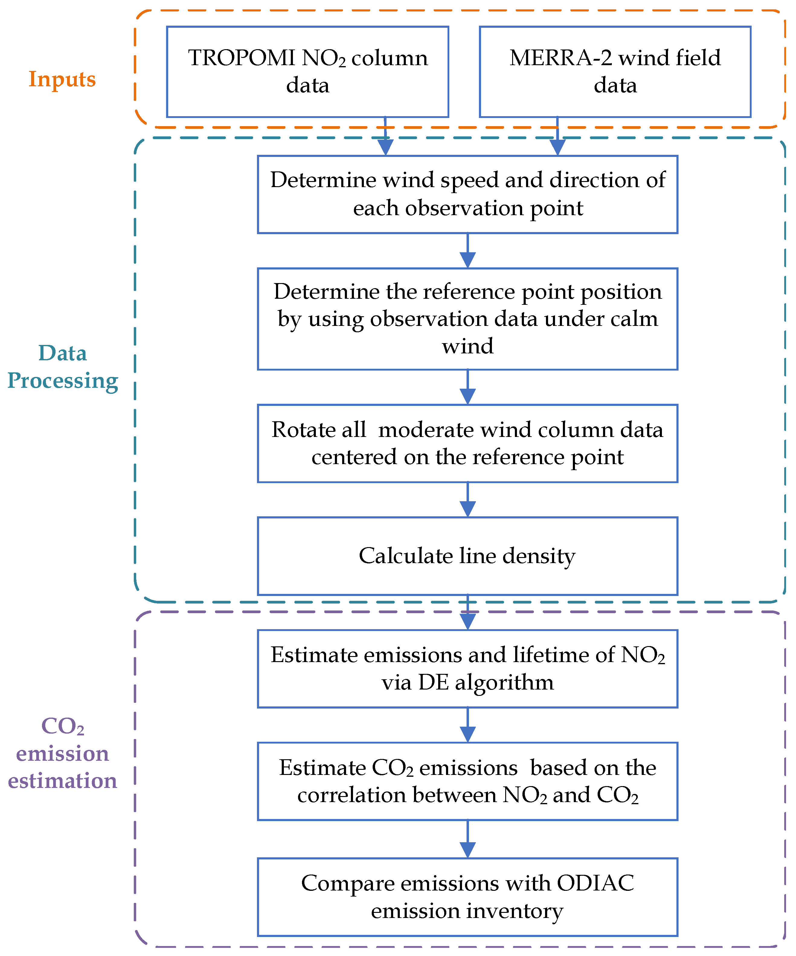
In this study, preprocessing was first performed on TROPOMI column data, MERRA-2 wind field data (M2I1NXASM), EDGAR (v8.0) and ODIAC 2024 emission inventory data. The observations were collocated with the wind field data based on temporal and geographic coordinates, assigning specific wind speed and direction to each data point. The emission center of was estimated using data under calm wind conditions (wind speed ≤ 3 m/s). Subsequently, data under moderate wind speeds (3–10 m/s) were rotated around this emission center and projected onto a standardized northerly wind direction. The line density distribution of the projected data was then calculated. A differential evolution algorithm (DE) was employed to estimate the emissions, lifetime, and background concentration that best fit the line density distribution. Finally, emissions were estimated based on the correlation between and . Figure 1 shows the schematic workflow of the proposed city-scale emission estimation framework.
2.1. TROPOMI Data
TROPOMI (TROPOspheric Monitoring Instrument) is a hyperspectral imager aboard the European Copernicus Sentinel 5 Precursor satellite, which was launched in October 2017. Its core mission is to observe the global tropospheric atmospheric composition with unprecedented spatial resolution, aiming to monitor air quality, the ozone layer and climate forcing factors. The payload is characterized by its extremely high spatial resolution, with a grid in nadir mode, which has been optimized to , significantly surpassing the previous generations of similar sensors (e.g., OMI). This allows TROPOMI to clearly identify emission hotspots such as cities, industrial zones, and even large point sources, laying the foundation for refined emission research [20,21,22].
Figure 1.
Schematic workflow of the proposed city-scale emission estimation framework. The process integrates multi-source data including TROPOMI column and MERRA-2 wind fields. Key methodological steps involve wind direction rotation for plume alignment, line density calculation, and the simultaneous retrieval of emissions and lifetimes using the differential evolution (DE) algorithm. Finally, emissions are estimated based on established – correlations and cross-compared with the ODIAC 2024 emission inventory.
TROPOMI’s high-precision column concentration data have been widely used in the derivation of high-spatial and high-temporal resolution emission inventories. Studies have shown that the emission estimates obtained using TROPOMI data are significantly higher in many rapidly developing regions compared to traditional bottom-up estimation methods, indicating potential systematic underestimations in the latter approach [23].
Additionally, leveraging the co-emission relationship between and , TROPOMI’s data have been successfully used as a “tracer” to estimate the emission flux of cities and point sources in combination with emission factors, providing a new method for independent cross-checking of carbon emissions [24,25,26].
Prior to analysis, TROPOMI tropospheric column data were filtered using rigorous quality control criteria: cloud radiance fraction ≤ 0.3, quality assurance (QA) value ≥ 0.7 (to balance data coverage and precision), solar zenith angle ≤ , and non-negative concentrations. To minimize the impact of extreme values, the interquartile range (IQR) method was employed to identify and remove daily observational outliers. The datasets were initially screened within a broad spatial domain (–N, –E) before being localized to the study areas. This comprehensive filtering process yielded a total of 105,324,377 valid observations across mainland China for the study period.
2.2. MERRA-2 Wind Field Data
The MERRA-2 reanalysis dataset was developed by NASA’s Global Modeling and Assimilation Office (GMAO) to provide comprehensive data on the atmosphere, land, and ocean. The MERRA-2 dataset is an important tool for climate research, weather forecasting, and air quality, including data from different altitude layers, such as humidity, wind speed, precipitation, etc., from the surface to the tropopause. Hourly, daily, and monthly wind field data is available for analysis and study of climate change, climate patterns, and long-term trends [27].
The data used in this study are the U50 and V50 wind speed data of the M2I1NXASM dataset in the MERRA-2 meteorological reanalysis data, and the wind speed components of U and V (east–west and north–south, respectively) are averaged in the vertical direction, with a resolution of and a temporal resolution of 1 h. To couple with TROPOMI’s column concentration data, the MERRA-2 wind speed data were interpolated onto a latitude and longitude grid of . In addition, the reanalysis data for 1 h was interpolated to obtain the vertical stratified wind speed and direction information at the TROPOMI transit time (about 13:30 h).
In this study, the MERRA-2 reanalysis product was selected primarily due to its high temporal resolution (1 h), which provides better alignment with the specific TROPOMI overpass times. While higher spatial resolution products or local meteorological station data were considered, MERRA-2 offers a consistent representation of wind fields well-suited for tracking the transport of tropospheric plumes. Local ground-based observations, although precise at the surface, often fail to represent the effective transport wind across the entire plume height due to surface friction and local turbulence. Therefore, the MERRA-2 wind field at a standardized near-surface level was utilized as a consistent proxy for regional-scale transport modeling. To ensure grid consistency with TROPOMI, the wind fields were remapped using bilinear interpolation, which serves as a spatial collocation operation without introducing additional sub-grid physical information.
2.3. Emission Inventory
EDGAR (Emissions Database for Global Atmospheric Research) is a global authoritative emissions inventory system developed by the European Commission’s Joint Research Centre (JRC) [28,29,30]. It provides the scientific community and policy makers with a set of independent, objective global data on human-induced emissions, characterized by extremely high spatial resolution. The core strength of EDGAR lies in the consistency of its methodology: it uses a unified data processing approach—mainly based on IPCC guidelines—to calculate emissions for all countries around the world, thereby eliminating potential inconsistencies that could arise from the different ways in which countries report their data.
EDGAR covers long series of data since 1970, including all greenhouse gases (GHGs), air pollutants and aerosols. Its data products typically provide high-resolution grid maps of country totals as well as , supporting a wide range of studies from global climate simulations to city-scale air quality forecasts.
The city-scale emissions derived in this study represent an integrated municipal-scale flux, which characterizes the cumulative strength of urban point, area, and line sources. This approach provides a macroscopic estimate of total urban activity rather than a fully source-resolved emission field.
In the latest versions, such as EDGAR v8.0, emissions are finely divided into fossil and bio :
- Fossil : A primary focus of the climate change research. EDGAR works closely with the International Energy Agency (IEA) to estimate emissions from data on industrial activities such as fuel combustion, cement production, metal fabrication and urea production.
- Biogenic : Mainly records carbon emissions from short-term biological cycles (such as biomass fuel combustion) and is often listed separately from fossil carbon in the inventory to better characterize measure carbon cycle impacts.
As a key air pollutant and ozone precursor, emissions are classified in EDGAR in an extremely detailed manner:
- Sectoral analysis: emissions data are highly dependent on combustion technology and end-of-line treatment measures (e.g., SCR denitrification). EDGAR documents emissions in the transport (especially road, aviation and shipping), the power industry and industrial thermal energy production in detail.
- Spatiotemporal characteristics: The database provides monthly or even hourly fluctuations in emissions, which is crucial for simulating regional acid rain, photochemical smog, and assessing the impact of air pollution control policies.
EDGAR is not only an important reference for the global stocktake under the Paris Agreement, but also provides a solid scientific basis for monitoring the global emission reduction process through the combination of satellite remote sensing and underlying statistics.
The Open-Data Inventory for Anthropogenic Carbon dioxide (ODIAC) provides a global high-resolution gridded dataset that quantifies fossil fuel combustion-derived emissions. This dataset innovatively integrates satellite nighttime light observations with emission inventories and geographic information of individual power plants, so as to precisely characterize the spatial distribution of national-scale fossil fuel emissions [31,32].
2.4. Emission Estimation Method
As a key meteorological factor affecting the diffusion and distribution of air pollutants, wind direction directly determines the transport path and deposition area of pollutants in the atmosphere. By analyzing data and determining the dominant trend of wind direction in a specific area, the dispersion pattern of pollutants can be effectively predicted, and then the main pollution source locations can be identified. The data analysis of the dominant wind direction can also help identify potential pollution accumulation areas, prevent and mitigate the occurrence of sudden air pollution events, and provide reliable basic data support for pollution source analysis. This is an important reference value for assessing the contribution of different emission sources to regional air quality and formulating scientific and reasonable pollution control strategies.
Beirle et al. [33] used wind field information to classify data in different downwind directions, and proposed a “line density” method to solve the problem of quantifying emissions from isolated urban sources. The basic assumption of this method is that urban emissions are regarded as approximate point source emissions. Based on satellite remote sensing data, the spatial distribution characteristics of column concentration around the city are mainly affected by the dual influence of point source emission transportation process and primary chemical reaction kinetics.
The introduction of the concept of ’line density’ aims to transform the two-dimensional distribution of concentration into a one-dimensional analysis problem. Before performing the wind-aligned coordinate transformation, a spatial reference point must be defined. In this study, rather than using the municipal administrative center, the reference point was determined based on the column concentration peak observed under calm wind conditions to more accurately represent the actual emission hotspot of each city. Following the coordinate rotation, the original two-dimensional average column volume distribution was simplified into a one-dimensional ‘line density’ representation by integrating the column volume along the cross-wind direction. To minimize potential interference and plume overlap from neighboring cities or industrial clusters, a focused integration sector with a width of 20 km (extending ±10 km from the central plume axis) was implemented. This simplified one-dimensional representation along the wind direction effectively captures the dominant urban emission signal while enhancing the robustness of the fitting process.
The model function (as a function of distance x) is used to fit the observed line density distribution, where E is the total emission; B is the background value of constant column concentration. x is the distance from the observation point to the effective emission center.
The exponential equation is an exponential function that describes the spatial distribution characteristics of atmospheric concentration around isolated cities and their distance-decay relationship with point source emissions under ideal conditions. X denotes the displacement of the emission source center relative to the nominal city center. In the downwind area, when , it is assumed that the pollutants diffuse linearly along the wind direction, and their attenuation process conforms to the first-order chemical reaction law, and the concentration in the urban periphery will decrease exponentially with the increase of distance. In the upwind region, i.e., , .
where is the e-folding distance, which refers to the distance spanned by the reduction of concentration to of the initial value. X is the displacement of the emission source center relative to the nominal city center; The mean lifetime is the quotient of the e-folding distance and the average wind speed downward of the target wind, as shown in the following Equation (3).
The Gaussian equation describes a Gaussian function with a standard deviation , which is used to describe the interference of different factors on the ideal distribution.
The factors affecting the ideal distribution are as follows: (1) Due to geographical location, the wind speed fluctuates in different locations; (2) because cities are not ideal point sources, their emissions present a certain degree of diffusion characteristics in the spatial range; and (3) secondary reaction processes such as photochemical reactions and oxidation reactions that may occur in the atmosphere will change their concentration and distribution characteristics, resulting in deviations between the actual distribution and the ideal distribution.
Under the combined influence of these interference factors, the actual distribution of emission sources in isolated cities is smoother than that of . Therefore, in the model, the actual distribution of around the city is regarded as the convolution result of and to reflect the influence of the above factors on .
The above parameters, including total emissions E, exponential attenuation distance , constant background concentration value B, emission source location X, and standard deviation of Gaussian function , are estimated by non-linear least squares fitting or other algorithms. Since least squares fitting (NLS) is prone to falling into the local minimum, a differential evolution (DE) optimization algorithm is used to estimate these parameters.
In order to efficiently utilize the remote sensing data collected by satellites, a data processing method based on wind direction rotation is adopted. The method uses the position of each TROPOMI pixel to be spatially rotated around the emission source, with the distance from the observation point to the emission source as the rotation radius, and the angle between the wind direction of the observation point and the reference wind direction as the rotation angle. During the data conversion process, the system maintains the wind speed values at each observation point unchanged, while adjusting the direction of wind at all data points to a consistent northward direction. This processing method not only retains the upwind–downwind spatial characteristics of the data points, but more importantly, realizes the unified analysis of the observation data under different wind direction conditions.
Recent advancements in satellite-based emission quantification have emphasized the importance of refined plume modeling. For instance, Tu et al. [34] successfully quantified emissions from coal mining areas in Shanxi by employing a wind-assigned anomaly method. While the line density model originated from point-source quantification, its application to city-scale emissions in this study is based on the “Integrated Source” approximation. In complex urban environments like those in Shandong, emissions from power plants (point), industrial zones (area), and transportation networks (line) often merge into a coherent downwind plume at the scale of the TROPOMI observations (approx. 5–7 km). By applying the DE algorithm, our framework does not assume a single mathematical point; instead, it optimizes the spatial distribution parameters to fit the integrated line density across the wind-aligned cross-sections. This approach effectively treats the urban agglomeration as an extended source with an optimized effective location and decay rate, a common practice in recent satellite-based urban inversions [35,36].
2.5. Differential Evolution Algorithm
The differential evolution algorithm takes the column concentration data and line density model treated by wind direction rotation as inputs, and sets key parameters such as emission flux, background concentration, e-folding distance, and Gaussian function standard deviation as optimization variables. Subsequently, the mutation, crossover, and selection operations are performed iteratively to minimize the difference between the simulated line density and the observed line density, and the optimal parameter set is output to reliably estimate emissions, laying the foundation for subsequent emission estimation.
Differential evolution (DE) is an efficient, population-based heuristic search algorithm proposed by Rainer Storn and Kenneth Price [37]. It is mainly used to solve the global optimization problem of continuous variables, and is popular because of its simple structure, few controlled parameters, and consistent performance in complex search spaces.
The line density model is characterized by high nonlinearity and multi-modality, making traditional gradient-based fitting prone to local optima. As a derivative-free global optimizer, DE has been utilized to identify parameters in atmospheric chemistry inverse modeling [38]. Furthermore, recent studies have highlighted its potential in improving the stability of carbon emission quantification [39].
The core idea of DE is to guide search by vector differences between individuals in a population. The process is divided into four main stages: initialization, mutation, crossover, and selection.
Initialization: As in any other evolutionary algorithm, the vectors of initial population of DE are generated randomly, and then evaluated. The ith individual vector of the population at generation g has D components.
Mutation: This is the essence of DE. The algorithm randomly selects three different individuals in the population, scales the difference between two of them, and synthesizes them with the third to generate a mutant vector . The most common mutation strategy (DE/rand/1) formula is as follows:
where F is the mutation scaling factor (usually between [0, 2]), and , , are different random integer indexes within .
Crossover: In order to increase population diversity, the mutant vector is recombined with the original target vector with a certain probability to generate the trial vector .
Selection: DE adopts a “greedy strategy”. Only if the trial vector is better suited than the current target vector will it make its way to the next generation:
The algorithm’s features include adaptability and ease of use. Adaptability: The size of the differential vector will automatically shrink with the convergence of the population, realizing the transition from global exploration to local exploitation. Simple and easy to use: usually only three parameters are required to adjust the population size , scaling factor F and crossover probability .
2.6. Study Area
Shandong Province is located on the eastern coast of China, in the lower Yellow River basin, and is an important strategic hinterland connecting Beijing-Tianjin-Hebei and the Yangtze River Delta. As one of the top three provinces in China’s total economy, Shandong is not only a major agricultural province, but also a core heavy industry base in the country.
Shandong Province has an extremely complete industrial system, covering high-energy-consuming industries such as refining, steel, aluminum and chemicals. This coal-based energy mix and highly concentrated heavy industry layout make it one of the provinces with the highest and emissions in China. The province’s electricity production is highly dependent on coal-fired thermal power, which provides an ideal observation scenario for using satellite data as a proxy indicator to quantify anthropogenic emissions. Shandong’s emission sources show the characteristics of “combination of point, line and area sources”. Point sources are the densely distributed coal-fired power plants and steel plants. Line sources are the traffic emissions generated by the busy Jiaoji railway and the highly developed highway network. Area sources are the human activities in metropolitan areas with Jinan and Qingdao as the core.
In the context of China’s carbon peaking and carbon neutrality goals, Shandong Province is in a critical period of transformation from high energy consumption to low-carbon. Using high-resolution satellite data such as TROPOMI, the emission changes of key cities in Shandong (such as Jinan, Qingdao, and Yantai) can be derived through the line density method, which can not only evaluate the consistency of the underlying emission inventory, but also provide complementary top-down support for assessing implementation effect of coal-control and emission reduction policies in the province in real time.
The selection of the study period (April to September 2022) is governed by the physical requirements of the -proxy method. First, the high spatial coverage of TROPOMI relative to current sensors allows for urban-scale analysis without complex interpolation. Second, the short atmospheric lifetime of during the non-heating season ensures that observed plumes are representative of localized anthropogenic emissions, minimizing the interference of regional transport. Crucially, this proxy approach effectively isolates fossil-fuel from biogenic sources, as and anthropogenic are co-emitted during combustion. By focusing on the photochemically active season, we circumvent the need for complex chemical transport models, thereby reducing the systematic uncertainties inherent in simulated meteorological and chemical mechanisms.
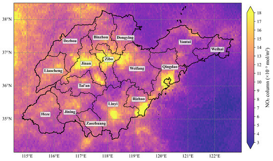
Figure 2 shows the spatial distribution of column concentrations in Shandong Province from April to September 2022, showing a pattern of “high in the west and central area and low in the eastern coast”, and the hotspot areas are highly consistent with the major industrial cities and urban agglomerations.
Figure 2.
Column distribution in Shandong Province during April to September of 2022.
The hotspot areas are mainly concentrated in central, western and southern Shandong, such as Jinan–Zibo–Weifang, Jining–Zaozhuang, and coastal cities such as Qingdao and Rizhao. These areas are the industrial, transportation and populated areas in Shandong Province, and emissions mainly come from industrial coal, motor vehicle exhaust and chemical production.
The areas with moderate concentrations cover most inland cities, such as Linyi, Dezhou, Liaocheng, Tai’an, etc., reflecting the local anthropogenic emission level.
The low-value areas are mainly distributed in the eastern coast of Shandong Province and some mountainous areas. These areas have low industrial density and better pollutant diffusion conditions due to the influence of marine climate, so the concentration is significantly lower.
In this study, seven cities (Jinan, Jining, Liaocheng, Linyi, Qingdao, Rizhao, and Yantai) were selected for carbon emission research in Shandong Province, as these cities have relatively high concentrations and are relatively isolated in location.
3. Results and Discussion
In this study, a data processing method based on wind direction rotation was adopted. The wind speed was divided into two categories for analysis. A calm wind condition was defined as wind speed ≤ 3 m/s, under which the spatial distribution of is dominated by local accumulation rather than horizontal advection. Moderate wind conditions were set to 3–10 m/s, which ensures stable pollutant advection and clear plume formation for emission estimation while avoiding extreme wind speeds (>10 m/s) that would cause rapid pollutant dilution and a significant decrease in the signal-to-noise ratio. The method first used the column concentration distribution under calm wind conditions to determine the reference point position. The position of each observation point under moderate wind speed is rotated in space centered on the reference point, the distance from the observation point to the emission source is the radius of rotation, and the angle between the wind direction of the observation point and the reference wind direction is the rotation angle. During the data conversion process, the system keeps the wind speed value of each observation point unchanged, and adjusts the wind direction of all points to a consistent northward direction. This processing method not only retains the upwind–downwind spatial characteristics of the data points, but more importantly, realizes the unified analysis of the observation data under different wind direction conditions.
3.1. Calculation of Line Density
While the line density model was originally designed for isolated emitters, its application here is justified through the ‘Integrated Source’ approximation. At TROPOMI resolution, diverse emission components within an urban area merge into a coherent downwind plume. Consequently, the DE optimization yields an effective source representation suitable for quantifying the overall municipal emission intensity, albeit without resolving individual industrial contributors.
Firstly, take Linyi City, Shandong Province, as an example for calculation. According to the 2023 Government Work Report of Linyi City, the prevailing wind direction in Linyi is northeasterly, with a corresponding wind direction frequency of 80%, and the average wind speed is 2.5 m/s.
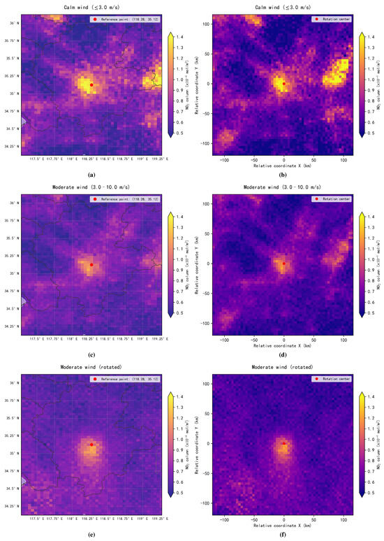
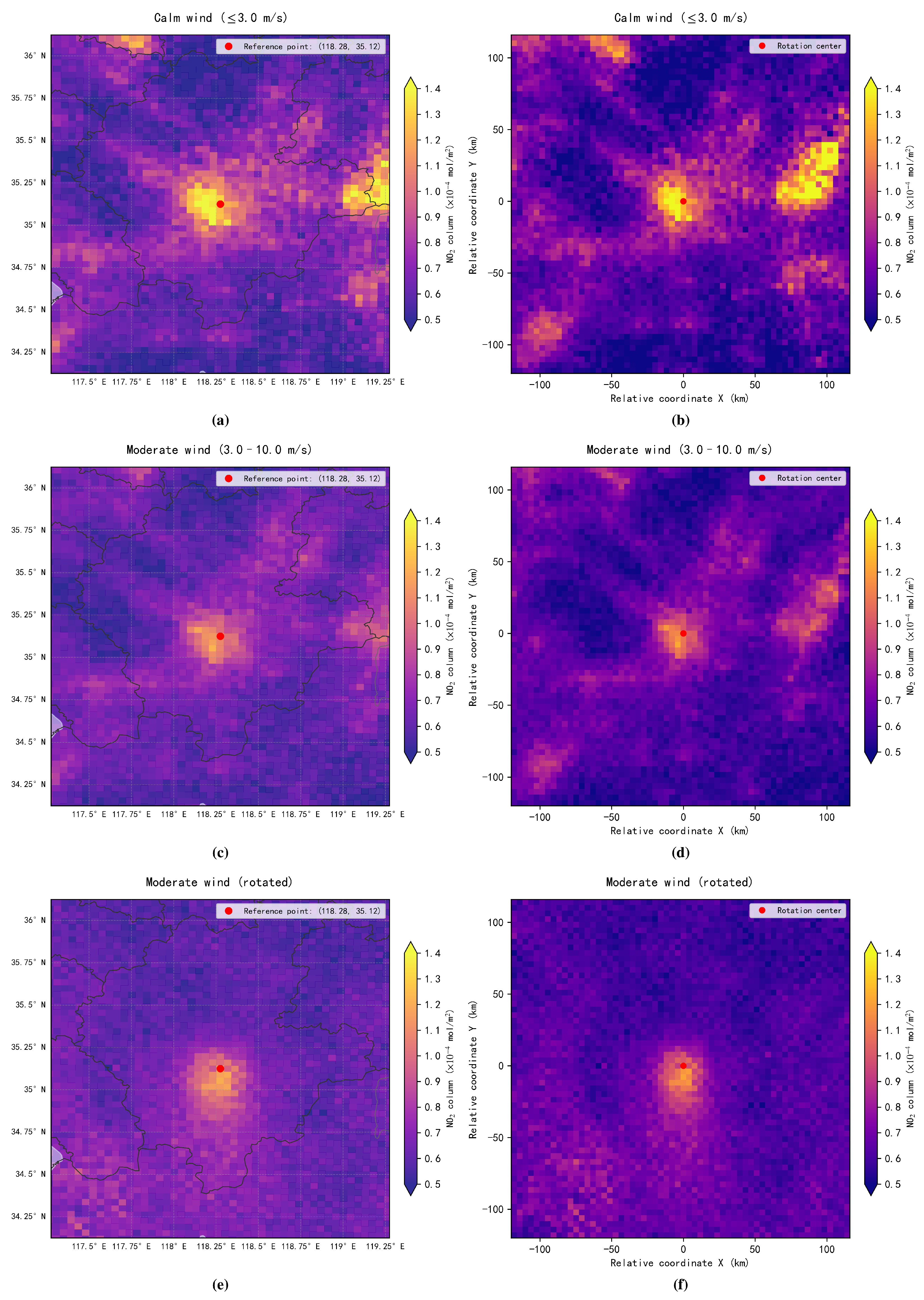
Figure 3 is a schematic diagram of wind direction rotation. Rotating wind direction eliminates the need to analyze the main wind direction of the study area by rotating all wind direction data to one wind direction. In the range of 120 km × 120 km in the study area, the grid resolution of 4 km × 4 km was adopted, and the area weight method was used for data processing.
Figure 3.
Schematic of the wind-rotation and coordinate-mapping process for Linyi. Left panels (a,c,e) show column concentrations under calm, moderate, and rotated-northward wind conditions in the original geographic coordinates. Right panels (b,d,f) display the corresponding distributions mapped onto a standardized Cartesian coordinate system centered at the emission source.
Figure 3a presents the spatial distribution characteristics of the average column concentration of in Linyi City under calm wind conditions from April to September 2022. It can be seen from the figure that the concentration value is spatially decreasing around a specific point. Figure 3c shows the spatial distribution of column concentration under moderate wind speed. Figure 3e exhibits the column concentration distribution when the data is for north-rotating wind conditions. It can be seen that the data for the north-rotating wind direction have the same wind direction, and are distributed in the upwind position (the positive half-axis of y-axis) and downwind position (the negative half-axis of y-axis), respectively, with obvious an northerly wind trend.
To improve the consistency of the emission characteristics, the column concentration data with latitude and longitude as the coordinates will be mapped to the Cartesian coordinate system centered on the reference point so as to realize the standardization of the wind direction of the observation data. Figure 3b,d,e show the spatial distribution pattern of column concentration in Linyi City after coordinate conversion.
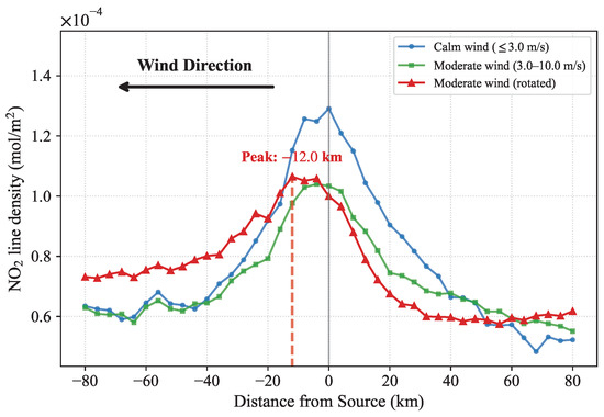
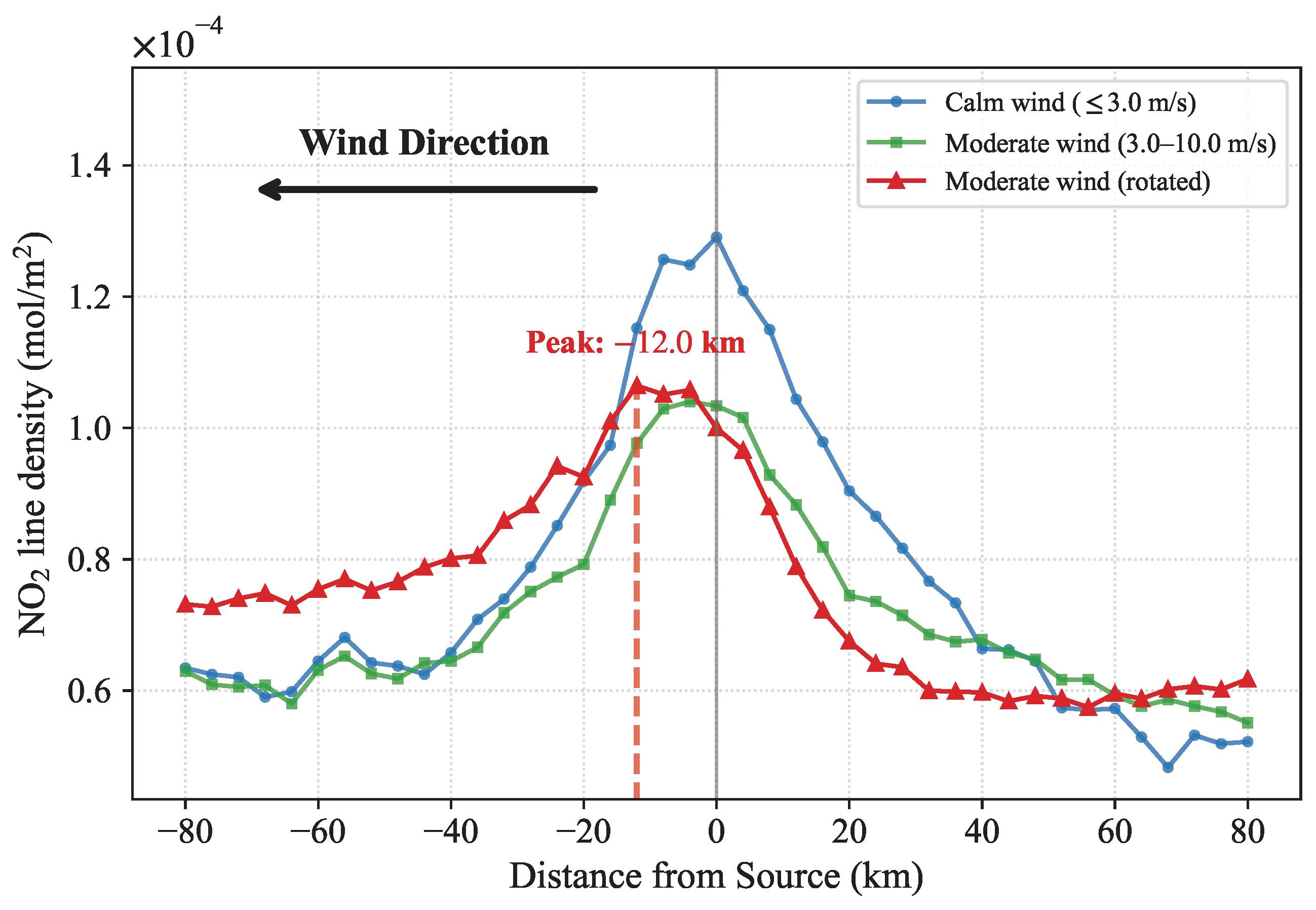
The calculated line density distribution is shown in Figure 4, which presents the line density under conditions of calm wind (blue line), moderate wind speed (green line) and northward-rotating wind (red line) in Linyi City, and the abscissa is the distance from the reference point, that is, the center of rotation. In calm wind conditions (blue line), the maximum value of line density () occurs in the effective emission center. The maximum line density () occurred 4 km south of the effective emission center under north-rotating wind. The line density in the upwind (areas with positive distance) gradually increases with closer to the emission source, and the change is steep. After peaking near the emission source (about −4 km), the line density begins to slowly decrease in the downwind (areas with negative distance), and the change is relatively flat, and finally stabilizes. The change in the position of the maximum line density under the conditions of calm wind and north-rotating wind reflects the diffusion range of the plume.
Figure 4.
Calculated line density distributions in Linyi under various wind conditions. The blue, green, and red lines represent calm wind, moderate wind, and rotated-northward wind conditions, respectively.
In this study, the differential evolution (DE) algorithm was employed for parameter optimization. To balance search breadth and convergence speed, key DE parameters were configured as follows: a total population size , a stochastic scaling factor , a crossover probability , and a maximum of 200 iterations. The process was governed by a termination tolerance of 0.01, ensuring both global exploration and computational efficiency.
The fitting results of the DE algorithm exhibit that the model parameters include emissions (E), background concentration (B), e-folding distance (), pollution source location relative to the nominal geographic center of Linyi (X), the mean () and the standard deviation () of the Gaussian function. The lower and upper limits for the six decision variables were set as and , representing the valid ranges of E, , , X, and B, respectively.
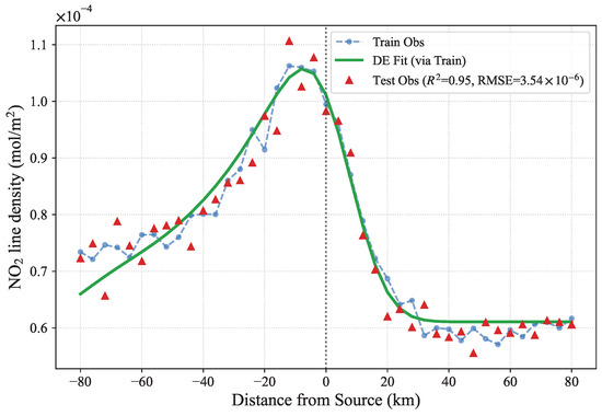
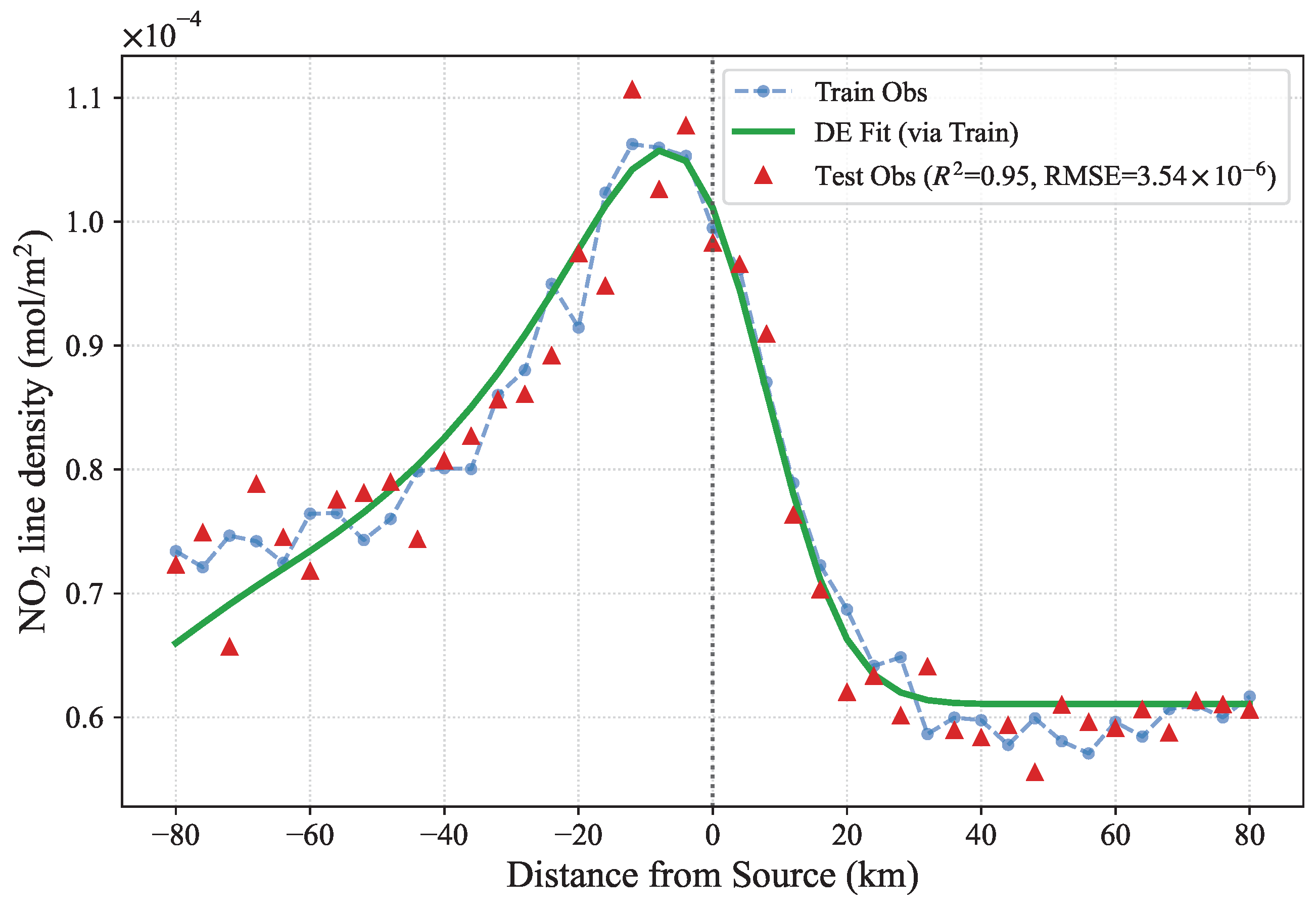
For Linyi City, there were 351,900 data points for moderate wind speeds during the study period. We randomly sampled 80% of the TROPOMI observations as a training set to reconstruct the line density curves and derive the six key parameters. The remaining 20% of the data was used as an independent test set to generate a separate set of observed line density. We then evaluated the model by comparing the fitting curve (derived from the training set) against the observed line density of the test set. As shown in Figure 5, the blue dashed line represents the line density observed from the training set, which were used to derive the six key parameters of the DE model. The solid green line presents the resulting fitting curve based on these training parameters. The red triangles indicate the observed line density from the independent test set. The high (0.95) and low () obtained on the test set indicate that the derived DE parameters exhibit high consistency and generalize well within the test dataset.
Figure 5.
Observed vs. DE-fitted line density for Linyi. Training observations (blue dashed line) were used for parameter optimization (green curve), while independent test observations (red triangles) were used to verify the consistency of the model estimates.
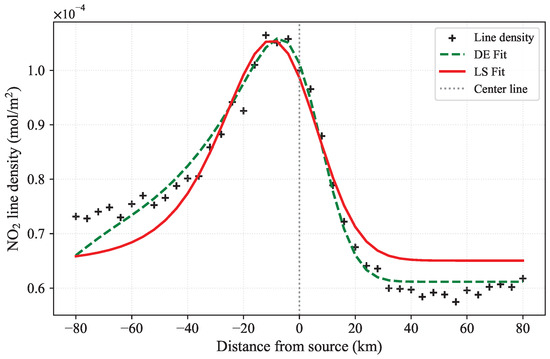
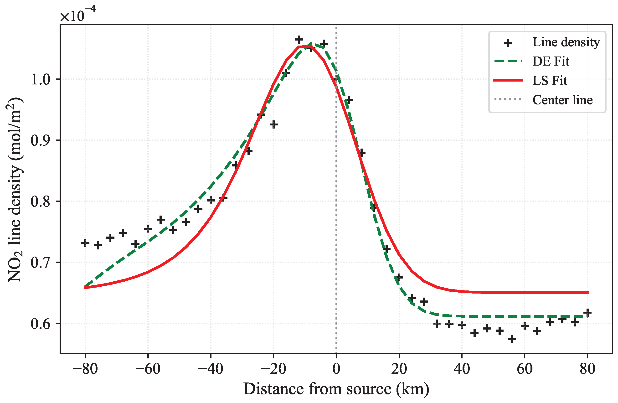
Figure 6 presents the fitting results of the line density model for Linyi City. The black crosses (+) represent the observed line density distribution derived from TROPOMI data after wind direction rotation. To evaluate the performance of the inversion framework, we compared the results of two optimization algorithms: the differential evolution (DE) algorithm (green dashed line) and the conventional non-linear least squares (LS) method (red solid line). The comparison reveals that the DE algorithm exhibits a better alignment to the observed data, particularly in capturing the peak enhancement near the source and the background concentration level, whereas the LS method exhibits a larger discrepancy in capturing the downwind decay gradient. Based on the DE-optimized parameters, the average emission rate for Linyi from April to September 2022 is estimated at . Furthermore, the atmospheric lifetime () is determined to be 5.08 h, derived from the ratio of the fitted e-folding distance () to the average wind speed ().
Figure 6.
Observed and fitted line density profiles for Linyi. Black crosses (+) denote wind-rotated TROPOMI observations. The green dashed line and red solid line represent fitting results using the differential evolution (DE) and non-linear least squares (LS) algorithms, respectively.
In the evaluation of column density fitting performance, the differential evolution (DE) algorithm exhibited enhanced stability and fitting consistency compared to the non-linear least squares (NLS) method. Specifically, the DE algorithm reduced the risk of the model falling into local optima during the simultaneous optimization of emission intensity and atmospheric lifetime, a common challenge for gradient-based NLS methods in non-linear line density fitting. Statistical results indicate that the DE algorithm achieved a high coefficient of determination (), whereas the NLS method only reached 0.896. Furthermore, the Root Mean Square Error (RMSE) for DE was merely , representing a reduction of approximately 48% compared to the NLS value of . These statistical discrepancies directly impact the reliability of the retrieved physical parameters. The NLS method yielded an unrealistically high emission estimate of 8926 tons per month and an excessively short atmospheric lifetime of 2.11 h, both of which are physically inconsistent with actual urban emission characteristics. In contrast, the DE algorithm, as a heuristic search method, effectively avoids the heavy dependence on initial values and the tendency to fall into local optima—common pitfalls for NLS. Consequently, DE exhibits improved physical consistency and greater inversion reliability within complex parameter spaces.
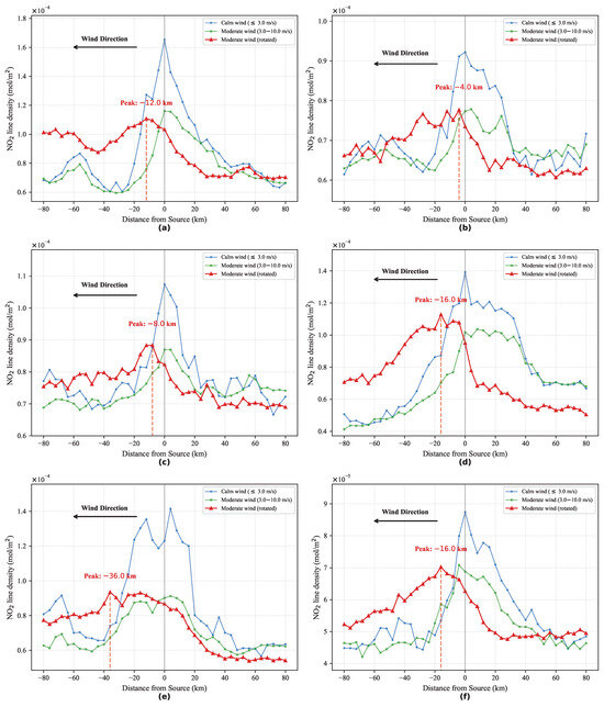
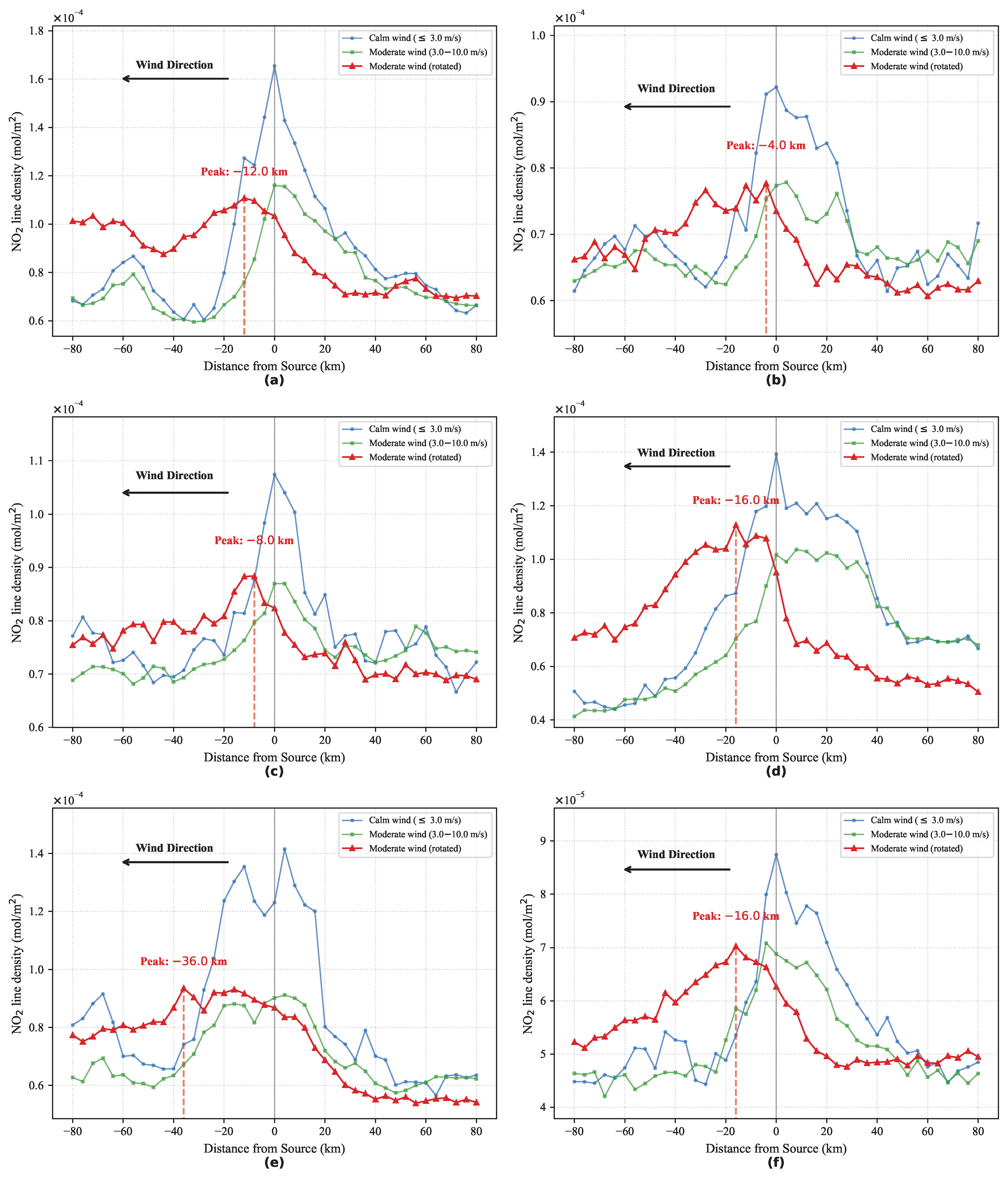
In addition, the line density was calculated for the other six cities in Shandong Province, including Jinan, Jining, Liaocheng, Qingdao, Rizhao and Yantai, under the conditions of calm wind (blue line), moderate wind speed (green line) and north-rotating wind (red line). Figure 7 shows the distribution of line density in the other six cities in Shandong Province. The results show that under calm wind conditions (blue line), the maximum value of line density occurs in the effective emission center. In the condition of north-rotating wind (red line), the maximum value of the line density occurs km south of the effective emission center. Similarly, the changes in the position of the maximum line density under calm wind and north-rotating wind conditions reflect the diffusion range of plumes in different urban areas.
Figure 7.
Calculated line density distributions in the other 6 cities under various wind conditions. The blue, green, and red lines represent calm wind, moderate wind, and north-rotated wind conditions, respectively. (a) Jinan, (b) Jining, (c) Liaocheng, (d) Qingdao, (e) Rizhao, (f) Yantai.
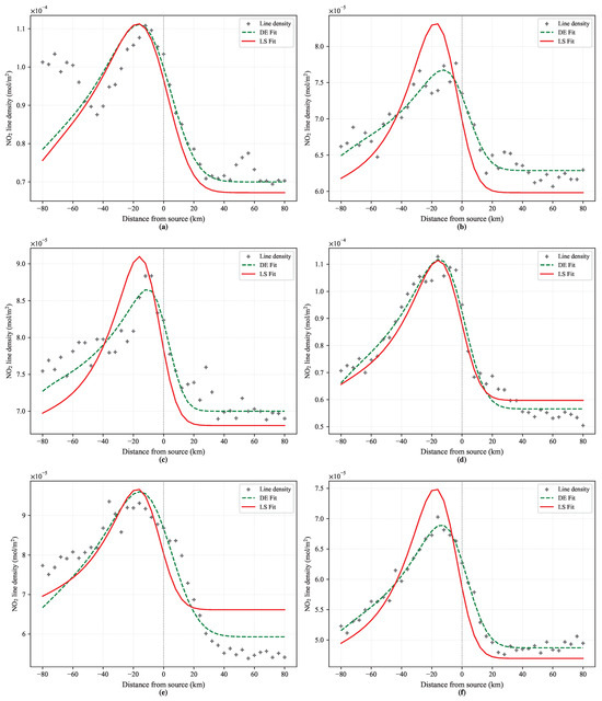
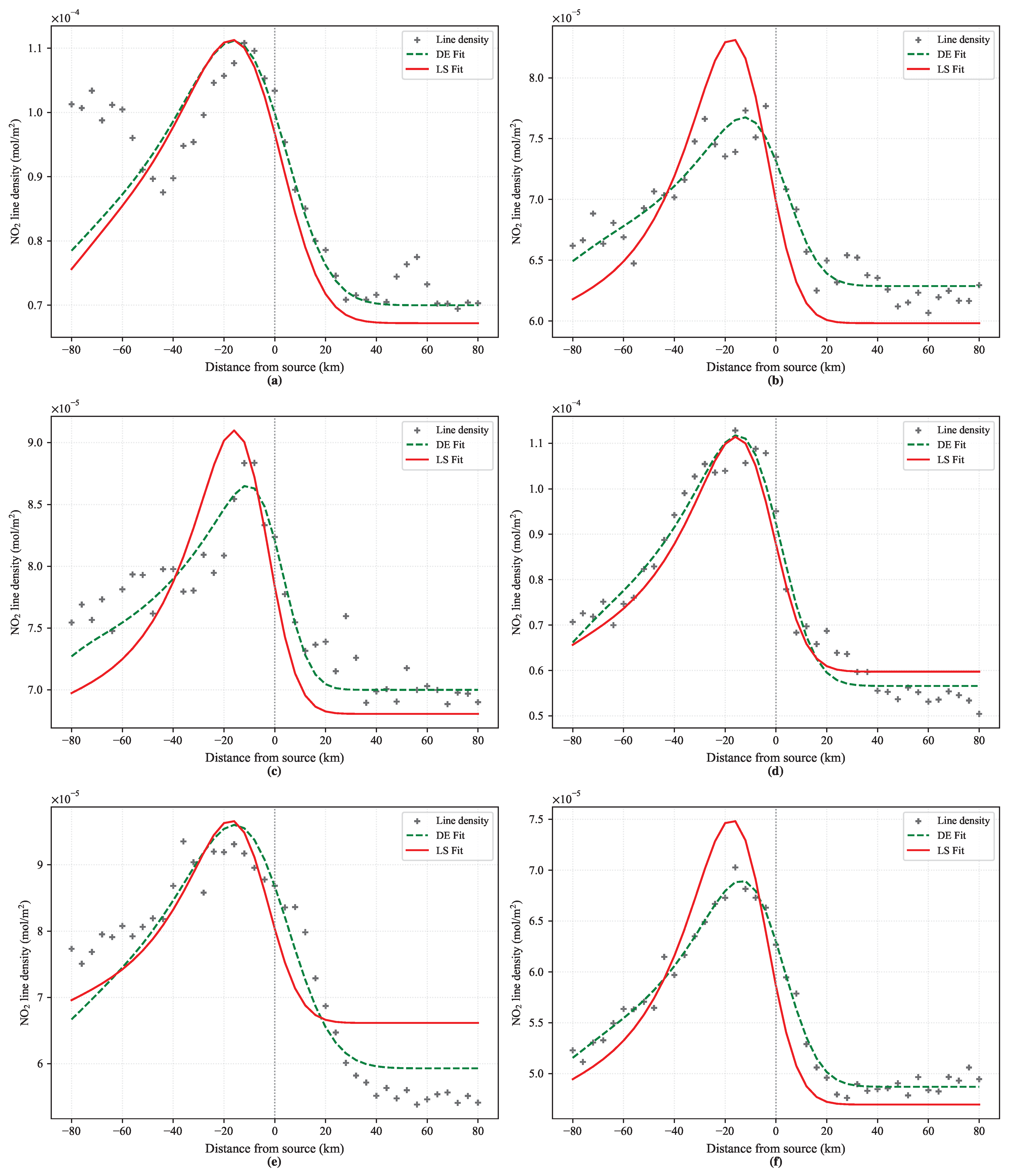
Figure 8 illustrates the line density model for the other six cities, fitted using both the DE and NLS algorithms. The black crosses (+) denote the observed line density obtained after wind direction rotation. The green dashed lines and red solid lines represent the fitting results using the differential evolution (DE) and non-linear least squares (NLS) methods, respectively. The observational data for these cities cover the same period from April to September 2022.
Figure 8.
Observed and fitted line density profiles in other 6 cities. Black crosses (+) denote wind-rotated TROPOMI observations. The green dashed lines and red solid lines represent fitting results using the differential evolution (DE) and non-linear least squares (LS) algorithms, respectively. (a) Jinan, (b) Jining, (c) Liaocheng, (d) Qingdao, (e) Rizhao, (f) Yantai.
3.2. Emission and Lifetimes
Table 1 summarizes the emission intensity () and atmospheric lifetimes (hours) of for seven cities in Shandong Province.
Table 1.
Estimated emissions and the lifetime of in seven cities in Shandong.
Qingdao has the highest emission intensity (), followed by Jinan () and Linyi (), indicating that these cities are the dominant emission sources in the region. In contrast, Jining () and Liaocheng () show relatively low emissions.
In terms of lifetime, Linyi exhibits a shorter lifetime (5.08 h), slightly lower than the 5.3 h presented in another study [36]. Despite its strong emissions, Linyi shows rapid chemical consumption and efficient horizontal dispersion under local meteorological conditions. Jinan and Rizhao show the longest lifetimes (5.56 h), suggesting weaker atmospheric diffusion and easier accumulation of pollutants. Other cities such as Yantai, Qingdao, Jining, and Liaocheng present a lifetime ranging from 4.9 h to 5.55 h.
Overall, the spatial differences in emission intensity in different cities reflect the heterogeneity of industrial and traffic sources, while the lifetime variations are mainly dominated by local meteorological conditions such as wind speed, boundary layer height, and photochemical activity.
3.3. Estimated Emissions and Comparison with Inventory
In this section, we evaluate the consistency of our city-scale emission estimates by comparing them with the ODIAC 2024 inventory. It is important to clarify that the emissions discussed herein specifically refer to anthropogenic fossil emissions, which include emissions from fossil fuel combustion and industrial processes. This dataset excludes biogenic from short-cycle biomass or large-scale biomass burning. Since is co-emitted with during fossil fuel combustion in urban environments, the TROPOMI -based inversion method is inherently most sensitive to fossil-origin carbon sources. This ensures a consistent physical basis for the comparison between our satellite-derived estimates and the ODIAC inventory.
This study obtains emission estimations based on statistical relationships. First, city-level and emission data are obtained from the EDGAR emission inventory. According to the photochemical equilibrium assumption widely used in satellite emissions studies, the conversion factor of 1.32 is used to convert emissions into emissions [33].
Then, a correlation between and emissions in the EDGAR inventory was established. Finally, based on the emissions derived from TROPOMI column concentrations using this relationship, emissions at the city scale were calculated.
In this study, a fixed conversion factor of 1.32 is adopted to estimate total emissions from TROPOMI columns. This value is based on the photochemical steady-state assumption under urban daytime conditions, a practical approximation widely utilized in comparable TROPOMI-based urban plume studies [33]. However, we acknowledge that the relationship is inherently dynamic and can vary with local chemical environments (e.g., and VOCs concentrations), transport time, and plume age. While a fixed ratio provides a consistent baseline for seasonal-scale regional comparisons, it may introduce localized biases compared to time-dependent or chemistry-transport model-based conversion treatments.
Table 2 compares the monthly averaged emissions derived from TROPOMI observations, the EDGAR emissions, the EDGAR emissions, estimated emissions, ODIAC emissions, and the ratio between the emissions estimated and ODIAC inventory across seven cities in Shandong Province.
Table 2.
Monthly averaged emission of and ().
Overall, Qingdao shows the highest TROPOMI-based emission (), followed by Jinan () and Linyi (), indicating that these cities are major emission hotspots in the region. In contrast, Jining exhibits the lowest emission, consistent with its relatively clean industrial structure.
For the estimated emissions, Jinan presents the largest value (), followed by Linyi () and Qingdao (). These cities also show high values in TROPOMI emissions, revealing a spatial consistency between and sources, which mainly come from industrial activities, fossil fuel combustion, and vehicle exhaust.
Cities such as Liaocheng, Jining, and Yantai show moderate levels in both observed and estimated emissions. As expected, Liaocheng displays lower emission levels, with the emission value of , which corresponds to the lower emissions. Due to the large ratio of emission and emission in Rizhao City in the EDGAR inventory, the lowest estimated carbon dioxide emissions among the seven cities were obtained in the case of higher estimated nitrogen dioxide emissions.
The ratios of estimated emissions and the emissions from the ODIAC inventory are between 0.51 and 1.01, with an average value of 0.74. Hence, the ODIAC inventory data across most cities overestimate the emissions. The relative consistency of estimated emissions with the inventory data supports the plausibility of our estimation method based on satellite observations.
3.4. Uncertainty Analysis and Difference Mechanism
This paper estimates the total uncertainty of satellite-derived emissions by formally propagating errors from multiple independent sources. Following the established frameworks of [33,40], the overall uncertainty () is calculated using the root-sum-squared (RSS) method, which assumes that individual error contributors are statistically independent:
The primary contributors to this error budget include:
- TROPOMI Inversion Error (): Based on official validation reports and external cross-comparisons, the precision of tropospheric column concentrations is estimated at 10–20%.
- Wind Field and Transport Error (): By comparing with MERRA-2 local data and performing sensitivity experiments, the overall transport uncertainty is estimated at 15–20%. This comprehensive budget accounts for deviations in wind speed and direction, as well as the specific bias arising from the selection of the 50 m wind (U50M) as the transport proxy.
- to Conversion Error (): Fluctuations in the Leighton ratio under varying photochemical conditions (, VOCs) introduce approximately 15% uncertainty, based on literature-based steady-state approximations.
- Differential Evolution (DE) Optimization Error (): The statistical fitting error of the DE algorithm is evaluated as the standard deviation of multiple optimization runs (with ) and is approximately 10%.
- Inventory-based Conversion Error (): Derived from sector-weighted emission factors in EDGAR, this remains the largest individual error source at approximately 25%.
By applying the RSS propagation formula, the combined city-scale uncertainty is estimated to be 35–45%. Since the conversion relationship is anchored to the EDGAR inventory, the ODIAC inventory functions as an external cross-comparison to assess the physical plausibility of the top-down results, rather than a fully independent absolute validation.
The observed discrepancies between our top-down estimates and the bottom-up inventories suggest several potential driving mechanisms.
First, the “ODIAC vs. EDGAR difference” represents a plausible interpretation of spatial proxy performance; the nighttime light-based proxy used in ODIAC appears to exhibit better spatial alignment with TROPOMI-observed plumes in the Shandong Industrial Corridor compared to the population-based allocation method employed by EDGAR. This may be because light-based proxies more effectively capture concentrated industrial clusters, whereas population density may not directly coincide with heavy industrial emission hotspots.
Second, localized variations in emission source structures—such as the contrast between modern power plants and areas dominated by high-density small-scale boilers—may lead to fluctuations in emission factors. These site-specific characteristics are only partially captured by generalized inventory-based coefficients, contributing to the observed deviations.
Finally, it must be noted that since our conversion relies on the relationship anchored to the EDGAR inventory, the comparison with ODIAC functions as a cross-comparison of spatial plausibility rather than a fully independent absolute validation. This exploratory framework serves to identify spatial discrepancies and provide top-down support for inventory refinement within the identified uncertainty ranges.
Furthermore, variations in the structure of emission sources—such as the contrast between modern power plants in Qingdao and high-density industrial areas dominated by small and medium-sized boilers elsewhere—could lead to localized fluctuations in emission factors. These site-specific characteristics are likely difficult to fully capture using generalized conversion methods, potentially contributing to the remaining discrepancies between top-down estimates and inventory data.
The choice of wind field height is a primary contributor to the budget. In this study, we utilized the MERRA-2 50 m wind (U50M, V50M) as a proxy for the transport of and plumes. While this level captures the horizontal advection near the emission sources, it may represent the lower bound of the effective transport wind speed, as plumes can extend to higher altitudes (e.g., 500 m) where wind speeds are typically higher. Based on the vertical wind profile characteristics in the study area, we estimate that the potential bias introduced by the wind height selection, along with the spatial remapping process, contributes approximately 10–15% to the transport-related uncertainty, forming the bulk of the estimated 15–20% total wind error.
to Conversion Error (): The assumption of a fixed conversion factor (1.32) introduces an estimated uncertainty of approximately 15%. As recent studies indicate that this relationship is sensitive to plume chemistry and meteorological variability, this factor is treated as a site-specific regional approximation rather than a universal constant. Its associated uncertainty is explicitly propagated into the total error budget to account for potential chemical regime shifts across different urban environments.
3.5. Applicability and Limitations
Although the framework constructed in this paper provides reliable top-down constraints for city-scale carbon emission estimation, several inherent limitations must be objectively recognized:
First, the method is highly sensitive to emission intensity and spatial proximity. The line density model relies on identifying significant plume enhancement signals above background concentrations; thus, it is most effective for high-intensity industrial clusters. In areas with lower emission intensity, background noise may interfere with fitting reliability. Additionally, in regions with closely distributed cities, such as the Jinan–Zibo corridor, the “isolated source” assumption may introduce spatial allocation biases. Overlapping plumes in such regions complicate background concentration segmentation, potentially leading to overestimation if signals from adjacent regions are not effectively separated.
Second, the results depend on the quality of meteorological fields and satellite retrievals. Wind field reliability directly affects the plume rotation and integration processes. The spatial resolution of MERRA-2 is relatively coarse compared to TROPOMI observations. Although bilinear interpolation enables grid matching, it cannot provide additional meteorological information at the sub-grid scale. This potential mismatch represents an ongoing source of uncertainty. Furthermore, satellite retrievals often face the challenge of underestimating near-surface , leading to systematic low biases in top-down estimates, as confirmed by recent global studies [35].
Third, the dependence of the derivation process on the EDGAR basal ratio is an inherent limitation of this study. Future improvements will require the introduction of direct observations such as OCO-3 to completely eliminate dependence on inventory scales.
Finally, there are limitations regarding the temporal scope and sectoral differentiation. This study focuses on the non-heating season (April–September) to utilize the short atmospheric lifetime of and minimize biogenic interference. Consequently, it does not cover the full annual cycle or heating-related emissions. Moreover, in the absence of auxiliary tracers, it remains difficult to distinguish specific emission sectors (e.g., transportation vs. industry) within a single urban plume. Future research could incorporate high-resolution spatial kernel functions and multi-species observational data to better characterize complex emission types and bridge the gap between global datasets and localized emission source depictions.
4. Conclusions
This study established a seasonal, satellite-constrained framework for the indirect estimation of city-scale emissions by integrating TROPOMI observations with a differential evolution (DE) optimized line density model. By focusing on the non-heating season (April–September 2022) to minimize confounding factors from domestic heating and complex photochemistry, the main conclusions are as follows:
First, the integration of multi-source data provides a viable approach for cross-verifying emission inventories. By combining high-resolution TROPOMI data with MERRA-2 refined wind fields, the framework enhances the identification of concentrated plume signals. The implementation of wind direction rotation and the DE algorithm effectively automates the simultaneous estimation of emissions and atmospheric lifetimes, providing a computationally efficient tool for regional-scale analysis.
Second, our results highlight significant spatial heterogeneity in emissions across Shandong Province. The identified hotspots in Qingdao, Linyi, and Jinan reflect the localized intensity of industrial activity. The estimated city-scale emissions exhibit higher spatial consistency with patterns and show plausible alignment with established inventories. The observed discrepancies between our top-down estimates and the ODIAC/EDGAR inventories suggest that spatial proxies (e.g., nighttime lights vs. population distribution) may significantly influence regional emission patterns. While our findings suggest that nighttime light-based proxies may align better with observed plumes in this industrial corridor, this remains a plausible inference derived from our observational evidence.
Third, this study acknowledges the inherent uncertainties in top-down inference. The total uncertainty (35–45%) is formally propagated from satellite inversion, wind field selection, and the inventory-anchored conversion ratio. Given the reliance on a fixed conversion factor and the seasonal specificity of the data, this framework should be viewed as a complementary diagnostic tool rather than a stand-alone policy-monitoring system.
In summary, the proposed method offers a valuable exploratory framework that provides top-down support for refining bottom-up inventories and identifying regional emission discrepancies. Future research integrating multi-seasonal data, time-dependent chemistry treatments, and direct observations (such as OCO-3) will be essential to further enhance the absolute accuracy and universal applicability of this top-down accounting solution for global carbon monitoring.
Author Contributions
Conceptualization, J.G. and Y.X.; methodology, Y.X.; software, Y.X.; validation, W.W., B.L. and Y.W.; formal analysis, Y.X.; investigation, Y.X.; resources, J.G.; data curation, Y.X.; writing—original draft preparation, Y.X. and C.D.; writing—review and editing, J.G. and Y.X.; visualization, Y.X.; supervision, J.G.; project administration, J.G.; funding acquisition, J.G. All authors have read and agreed to the published version of the manuscript.
Funding
This research was funded by the Jing-Jin-Ji Regional Integrated Environmental Improvement-National Science and Technology Major Project of Ministry of Ecology and Environment of China (2025ZD1200700), the Open Foundation of Kunyu Mountain Ecological Quality Comprehensive Monitoring Station, Ministry of Ecology and Environment, PRC (NIES-KYS-202501) and the Special Fund of Chinese Central Government for Basic Scientific Research Operations in Commonweal Research Institute (GYZX250103, GYZX250208, GYZX250209).
Institutional Review Board Statement
Not applicable.
Informed Consent Statement
Not applicable.
Data Availability Statement
All datasets used in this study are publicly available. The S5P/TROPOMI observations are available at https://dataspace.copernicus.eu (accessed on 1 May 2026). MERRA-2 reanalysis data are available at https://disc.gsfc.nasa.gov (accessed on 1 May 2026). The EDGAR emission inventory is available at https://edgar.jrc.ec.europa.eu/dataset_ghg80 (accessed on 1 May 2026).
Acknowledgments
The authors would like to thank the European Space Agency (ESA) for providing TROPOMI data, NASA for providing MERRA-2 reanalysis data, and the European Commission’s Joint Research Centre (JRC) for providing EDGAR emission inventory.
Conflicts of Interest
The authors declare no conflicts of interest. The funders had no role in the design of the study; in the collection, analyses, or interpretation of data; in the writing of the manuscript; or in the decision to publish the results.
Abbreviations
The following abbreviations are used in this manuscript:
| DE | Differential Evolution |
| EDGAR | Emissions Database for Global Atmospheric Research |
| ESA | European Space Agency |
| GMAO | Global Modeling and Assimilation Office |
| IPCC | Intergovernmental Panel on Climate Change |
| JRC | Joint Research Centre |
| MERRA-2 | Modern-Era Retrospective analysis for Research and Applications, Version 2 |
| NASA | National Aeronautics and Space Administration |
| ODIAC | Open-Data Inventory for Anthropogenic Carbon dioxide |
| TROPOMI | TROPOspheric Monitoring Instrument |
References
- Friedlingstein, P.; O’Sullivan, M.; Jones, M.W.; Andrew, R.M.; Gregor, L.; Hauck, J.; Le Quéré, C.; Luijkx, I.T.; Olsen, A.; Peters, G.P.; et al. Global Carbon Budget 2022. Earth Syst. Sci. Data 2022, 14, 4811–4900. [Google Scholar] [CrossRef] [Scilit]
- Intergovernmental Panel on Climate Change (IPCC). Climate Change 2021—The Physical Science Basis: Working Group I Contribution to the Sixth Assessment Report of the Intergovernmental Panel on Climate Change; Cambridge University Press: Cambridge, UK, 2023; Available online: https://digitallibrary.un.org/record/3934600?v=pdf (accessed on 19 March 2026).
- Satterthwaite, D. Cities’ contribution to global warming: Notes on the allocation of greenhouse gas emissions. Environ. Urban. 2008, 20, 539–549. [Google Scholar] [CrossRef] [Scilit]
- Andres, R.J.; Boden, T.A.; Bréon, F.-M.; Ciais, P.; Davis, S.; Erickson, D.; Gregg, J.S.; Jacobson, A.; Marl, G.; Miller, J.; et al. A synthesis of carbon dioxide emissions from fossil-fuel combustion. Biogeosciences 2012, 9, 1845–1871. [Google Scholar] [CrossRef] [Scilit]
- Zheng, B.; Chevallier, F.; Ciais, P.; Broquet, G.; Wang, Y.; Lian, J.; Zhao, Y. Observing carbon dioxide emissions over China’s cities and industrial areas with the Orbiting Carbon Observatory-2. Atmos. Chem. Phys. 2020, 20, 8501–8510. [Google Scholar] [CrossRef] [Scilit]
- Liu, F.; Beirle, S.; Joiner, J.; Choi, S.; Tao, Z.; Knowland, K.E.; Smith, S.J.; Tong, D.Q.; Ma, S.; Fasnacht, Z.T.; et al. High-resolution mapping of nitrogen oxide emissions in large US cities from TROPOMI retrievals of tropospheric nitrogen dioxide columns. Atmos. Chem. Phys. 2024, 24, 3717–3728. [Google Scholar] [CrossRef] [Scilit]
- Rey-Pommier, A.; Héraud, A.; Chevallier, F.; Ciais, P.; Christoudias, T.; Kushta, J.; Sciare, J. Global gridded NOx emissions using TROPOMI observations. Earth Syst. Sci. Data 2025, 17, 3329–3351. [Google Scholar] [CrossRef] [Scilit]
- Pommier, M. Estimations of NOx emissions, NO2 lifetime and their temporal variation over three British urbanised regions in 2019 using TROPOMI NO2 observations. Environ. Sci. Atmos. 2023, 3, 408–421. [Google Scholar] [CrossRef] [Scilit]
- Lange, K.; Richter, A.; Burrows, J.P. Variability of nitrogen oxide emission fluxes and lifetimes estimated from Sentinel-5P TROPOMI observations. Atmos. Chem. Phys. 2022, 22, 2745–2767. [Google Scholar] [CrossRef] [Scilit]
- Luo, Z.; He, T.; Yi, W.; Zhao, J.; Zhang, Z.; Wang, Y.; Liu, H.; He, K. Advancing shipping NOx pollution estimation through a satellite-based approach. PNAS Nexus 2024, 3, pgad430. [Google Scholar] [CrossRef] [Scilit] [PubMed]
- Oda, T.; Maksyutov, S. ODIAC Fossil Fuel CO2 Emissions Dataset (Version: ODIAC2024); Center for Global Environmental Research, National Institute for Environmental Studies: Tsukuba, Japan, 2015. [CrossRef]
- Li, H.; Qin, K.; Li, D.; Wang, L.; He, Q.; Cohen, J.B. Monitoring fossil fuel CO2 emissions from co-emitted NO2 observed from space: Progress, challenges, and future perspectives. Front. Environ. Sci. Eng. 2024, 19, 2. [Google Scholar] [CrossRef] [Scilit]
- McDuffie, E.E.; Smith, S.J.; O’Rourke, P.; Tibrewal, K.; Venkataraman, C.; Marais, E.A.; Zheng, B.; Crippa, M.; Brauer, M.; Martin, R.V. A global anthropogenic emission inventory of atmospheric pollutants from sector- and fuel-specific sources (1970–2017). Earth Syst. Sci. Data 2020, 12, 3413–3442. [Google Scholar] [CrossRef] [Scilit]
- Yang, E.G.; Kort, E.A.; Ott, L.E.; Oda, T.; Lin, J.C. Using Space-Based CO2 and NO2 Observations to Estimate Urban CO2 Emissions. J. Geophys. Res. Atmos. 2023, 128, e2022JD037736. [Google Scholar] [CrossRef] [Scilit]
- Fioletov, V.; McLinden, C.A.; Griffin, D.; Krotkov, N.; Liu, F.; Eskes, H. Global seasonal urban, industrial, and background NO2 estimated from TROPOMI satellite observations. Atmos. Chem. Phys. 2025, 25, 575–596. [Google Scholar] [CrossRef] [Scilit]
- Reuter, M.; Buchwitz, M.; Schneising, O.; Krautwurst, S.; O’Dell, C.W.; Richter, A.; Bovensmann, H.; Burrows, J.P. Towards monitoring localized CO2 emissions from space: Co-located regional CO2 and NO2 enhancements observed by the OCO-2 and S5P satellites. Atmos. Chem. Phys. 2019, 19, 9371–9383. [Google Scholar] [CrossRef] [Scilit]
- Zhang, Q.; Liu, Y.; Wang, T.; Zhang, X.; Kang, S.; Chen, B. Quantifying daily NOx and CO2 emissions from Wuhan using satellite observations from TROPOMI and OCO-2. Atmos. Chem. Phys. 2023, 23, 551–563. [Google Scholar] [CrossRef] [Scilit]
- Liu, F.; Duncan, B.N.; Krotkov, N.A.; Lamsal, L.N.; Beirle, S.; Griffin, D.; McLinden, C.A.; Goldberg, D.L.; Lu, Z. A methodology to constrain carbon dioxide emissions from coal-fired power plants using satellite observations of co-emitted nitrogen dioxide. Atmos. Chem. Phys. 2020, 20, 99–116. [Google Scholar] [CrossRef] [Scilit]
- Schooling, C.N.; Feng, L.; Super, I.; Palmer, P.I. Inferring European Fossil Fuel CO2 Emissions using TROPOMI NO2 Data and Sector-Based NOx:CO2 Emission Ratios. EGUsphere 2026, 2026, 1–23. [Google Scholar] [CrossRef] [Scilit]
- Veefkind, J.P.; Aben, I.; McMullan, K.; Förster, H.; de Vries, J.; Otter, G.; Claas, J.; Eskes, H.J.; de Haan, J.F.; Kleipool, Q.; et al. TROPOMI on the ESA Sentinel-5 Precursor: A GMES mission for global observations of the atmospheric composition for climate, air quality and ozone layer applications. Remote Sens. Environ. 2012, 120, 70–83. [Google Scholar] [CrossRef] [Scilit]
- Van Geffen, J.; Boersma, K.F.; Eskes, H.; Sneep, M.; ter Linden, M.; Zara, M.; Veefkind, J.P. S5P TROPOMI NO2 slant column retrieval: Method, stability, uncertainties and comparisons with OMI. Atmos. Meas. Tech. 2020, 13, 1315–1335. [Google Scholar] [CrossRef] [Scilit]
- Copernicus Sentinel-5P; European Space Agency (ESA). TROPOMI Level 2 Nitrogen Dioxide Total Column Products (Version 02); European Space Agency (ESA): Paris, France, 2021. [Google Scholar] [CrossRef] [Scilit]
- Kong, Y.; Wang, Y.; Zhang, X.; Li, R.; Chen, J. Tracking daily NOx emissions from an urban agglomeration based on TROPOMI NO2 and a local ensemble transform Kalman filter. Atmos. Chem. Phys. 2025, 25, 5959–5976. [Google Scholar] [CrossRef] [Scilit]
- Jia, Y.; Liu, C.; Xing, C.; Hu, Q.; Tan, W. Estimating daily NOx and CO2 emissions in typical megacities of east China using TROPOMI NO2 observations. Atmos. Environ. 2025, 359, 121377. [Google Scholar] [CrossRef] [Scilit]
- Fuentes Andrade, B.; Buchwitz, M.; Reuter, M.; Bovensmann, H.; Richter, A.; Boesch, H.; Aben, I. A method for estimating localized CO2 emissions from co-located satellite XCO2 and NO2 images. Atmos. Meas. Tech. 2024, 17, 1145–1173. [Google Scholar] [CrossRef] [Scilit]
- Santaren, D.; Broquet, G.; Bréon, F.M.; Chevallier, F.; Kuhlmann, G.; Marshall, J. Benchmarking data-driven inversion methods for the estimation of local CO2 emissions from synthetic satellite images of XCO2 and NO2. Atmos. Meas. Tech. 2025, 18, 211–239. [Google Scholar] [CrossRef] [Scilit]
- Gelaro, R.; McCarty, W.; Suárez, M.J.; Todling, R.; Molod, A.; Takacs, L.; Randles, C.A.; Darmenov, A.; Bosilovich, M.G.; Reichle, R.; et al. The Modern-Era Retrospective Analysis for Research and Applications, Version 2 (MERRA-2). J. Clim. 2017, 30, 5419–5454. [Google Scholar] [CrossRef] [Scilit] [PubMed]
- Crippa, M.; Guizzardi, D.; Pagani, F.; Banja, M.; Muntean, M.; Schaaf, E.; Monforti-Ferrario, F.; Banja, M.; Olivier, J.G.J.; Grassi, G.; et al. GHG Emissions of All World Countries; JRC Scientific and Policy Report; Publications Office of the European Union: Luxembourg, 2024. [Google Scholar] [CrossRef]
- Crippa, M.; Guizzardi, D.; Pagani, F.; Schiavina, M.; Melchiorri, M.; Pisoni, E.; Graziosi, F.; Muntean, M.; Maes, J.; Dijkstra, L.; et al. Insights into the spatial distribution of global, national, and subnational greenhouse gas emissions in the Emissions Database for Global Atmospheric Research (EDGAR v8.0). Earth Syst. Sci. Data 2024, 16, 2811–2830. [Google Scholar] [CrossRef] [Scilit]
- Banja, M.; Crippa, M.; Guizzardi, D.; Rossi, S.; Pagani, F.; Muntean, M.; Schaaf, E. A comparative analysis of EDGAR and UNFCCC GHG emissions inventories: Insights on trends, methodology and data discrepancies. Earth Syst. Sci. Data 2025, 17, 6461–6486. [Google Scholar] [CrossRef] [Scilit]
- Oda, T.; Maksyutov, S. A very high-resolution (1 km × 1 km) global fossil fuel CO2 emission inventory derived using a point source database and satellite observations of nighttime lights. Atmos. Chem. Phys. 2011, 11, 543–556. [Google Scholar] [CrossRef] [Scilit]
- Oda, T.; Maksyutov, S.; Andres, R.J. The Open-source Data Inventory for Anthropogenic CO2, version 2016 (ODIAC2016): A global monthly fossil fuel CO2 gridded emissions data product for tracer transport simulations and surface flux inversions. Earth Syst. Sci. Data 2018, 10, 87–107. [Google Scholar] [CrossRef] [Scilit]
- Beirle, S.; Boersma, K.F.; Platt, U.; Lawrence, M.G.; Wagner, T. Megacity Emissions and Lifetimes of Nitrogen Oxides Probed from Space. Science 2011, 333, 1737–1739. [Google Scholar] [CrossRef] [Scilit]
- Tu, Q.; Hase, F.; Qin, K.; Cohen, J.B.; Khosrawi, F.; Zou, X.; Schneider, M.; Lu, F. Quantifying CH4 emissions from coal mine aggregation areas in Shanxi, China, using TROPOMI observations and the wind-assigned anomaly method. Atmos. Chem. Phys. 2024, 24, 4875–4894. [Google Scholar] [CrossRef] [Scilit]
- Beirle, S.; Borger, C.; Dörner, S.; Eskes, H.; Kumar, V.; de Laat, A.; Wagner, T. Catalog of NOx emissions from point sources as derived from the divergence of the NO2 flux for TROPOMI. Earth Syst. Sci. Data 2021, 13, 2995–3012. [Google Scholar] [CrossRef] [Scilit]
- Liu, F.; Beirle, S.; Zhang, Q.; Dörner, S.; He, K.; Wagner, T. NOx lifetimes and emissions of cities and power plants in polluted background estimated by satellite observations. Atmos. Chem. Phys. 2016, 16, 5283–5298. [Google Scholar] [CrossRef] [Scilit]
- Storn, R.; Price, K. Differential Evolution—A Simple and Efficient Heuristic for global Optimization over Continuous Spaces. J. Glob. Optim. 1997, 11, 341–359. [Google Scholar] [CrossRef] [Scilit]
- Penenko, A.V.; Konopleva, V.S.; Penenko, V.V. Inverse modeling of atmospheric chemistry with a differential evolution solver: Inverse problem and Data assimilation. IOP Conf. Ser. Earth Environ. Sci. 2022, 1023, 012015. [Google Scholar] [CrossRef] [Scilit]
- Zhang, L.; Lu, G.; Yan, X.; Xia, P.; Chen, Z.; Wu, D. A differential evolution optimized hybrid XGBoost for accurate carbon emission prediction. Environ. Model. Softw. 2025, 193, 106627. [Google Scholar] [CrossRef] [Scilit]
- Zheng, B.; Cohen, J.B.; Lu, L.; Hu, W.; Tiwari, P.; Lolli, S.; Garzelli, A.; Su, H.; Qin, K. How can we trust TROPOMI based methane emissions estimation: Calculating emissions over unidentified source regions. Atmos. Chem. Phys. 2026, 26, 1931–1946. [Google Scholar] [CrossRef] [Scilit]

Disclaimer/Publisher’s Note: The statements, opinions and data contained in all publications are solely those of the individual author(s) and contributor(s) and not of MDPI and/or the editor(s). MDPI and/or the editor(s) disclaim responsibility for any injury to people or property resulting from any ideas, methods, instructions or products referred to in the content. |
© 2026 by the authors. Licensee MDPI, Basel, Switzerland. This article is an open access article distributed under the terms and conditions of the Creative Commons Attribution (CC BY) license.