


Abstract
The advent of satellite-borne machine learning hardware accelerators has enabled the onboard processing of payload data using machine learning techniques such as convolutional neural networks (CNNs). A notable example is using a CNN to detect the presence of clouds in the multispectral data captured on Earth observation (EO) missions, whereby only clear sky data are downlinked to conserve bandwidth. However, prior to deployment, new missions that employ new sensors will not have enough representative datasets to train a CNN model, while a model trained solely on data from previous missions will underperform when deployed to process the data on the new missions. This underperformance stems from the domain gap, i.e., differences in the underlying distributions of the data generated by the different sensors in previous and future missions. In this paper, we address the domain gap problem in the context of onboard multispectral cloud detection. Our main contributions lie in formulating new domain adaptation tasks that are motivated by a concrete EO mission, developing a novel algorithm for bandwidth-efficient supervised domain adaptation, and demonstrating test-time adaptation algorithms on space deployable neural network accelerators. Our contributions enable minimal data transmission to be invoked (e.g., only 1% of the weights in ResNet50) to achieve domain adaptation, thereby allowing more sophisticated CNN models to be deployed and updated on satellites without being hampered by domain gap and bandwidth limitations.
1. Introduction
Space provides a useful vantage point for monitoring large-scale trends on the surface of the Earth. For that reason, numerous Earth observation (EO) satellite missions have been launched or are being planned. By Novaspace’s estimate [1], the number of EO satellites will grow by 190% between 2024 and 2033. Typical EO satellites carry multispectral or hyperspectral sensors that measure the electromagnetic radiations emitted or reflected from the surface, which are then processed to form data cubes. These data cubes are the valuable inputs to various EO applications.
Many EO satellites also process the data captured by the multi/hyperspectral imagers, however, this has hitherto been limited to low-level preprocessing tasks, such as data enhancement and compression. Recently, the advent of satellite-borne hardware accelerators for machine learning inference has opened up the possibility of more advanced processing. A notable example is the PhiSat-1 mission [2], which carries the HyperScout-2 payload [3]. The payload consists of a hyperspectral imager and the Eyes of Things (EoT) “AI on-board” [4], which executes a convolutional neural network (CNN) called CloudScout [5,6] to perform cloud detection on the collected EO measurements. The result informs whether the geographic area in the field of view is under significant cloud cover, and only clear-sky data cubes are downlinked to optimise bandwidth utilisation.
Generally speaking, new missions that employ new sensors (e.g., HyperScout 2) typically do not have enough representative datasets to train a CNN model. An intuitive solution is to use data captured from a previous satellite mission to train the model (e.g., the CloudScout model was trained on data from Sentinel-2 [5,7]). This workaround, however, will introduce another problem called domain gap or domain shift [8], whereby the seemingly similar data from the training and testing domains actually differ significantly in their underlying distributions. The domain gap problem will cause the trained CNNs to perform poorly in the deployed environment. Section 1.1 and Section 1.2 describe the domain gap problem in the context of satellite-borne machine learning in more detail.
1.1. What Is the Domain Gap Problem?
The domain gap refers to the difference between the distribution of source-domain data (or simply source data, i.e., data used for training a model) and the distribution of target-domain data (or simply target data, i.e., data encountered in the field). This gap arises from a shift in the target distribution relative to the source distribution, i.e.,
- deviating from in what is known as the covariate shift,
- or less commonly, deviating from , or deviating from ,
where the subscripts s and t denote the source and target domains, x and y denote data and label, respectively. For a significant domain gap, a model that performs well on the source data may fail to generalise to target data; see Figure 1. The domain gap thus poses a fundamental problem that challenges the general performance of machine learning techniques.
Figure 1.
An illustration of the the multispectral domain gap problem. Every multispectral image is a multidimensional data point. A cloud detector maps each of these multidimensional data points to a binary cloudy/non-cloudy label. To facilitate visualisation, each image is represented by a two-dimensional data point. For images in the Sentinel-2 domain, for example, the left plot shows a hypothetical data distribution, based on whether a Sentinel-2-trained cloud detector classifies images as cloudy (‘x’) or noncloudy (‘o’). The Sentinel-2-trained cloud detector would, however, be poor at distinguishing the cloudy (‘x’) and noncloudy (‘o’) images distributed in the right plot, which visualises the hypothetical data distribution for Landsat 9. In the figure above, without domain adaptation, a Sentinel-2-trained cloud detector correctly classifies the sample cloudy image on the left but incorrectly classifies the sample cloudy image on the right. See Section 8.1 for quantitative results confirming the presence of multispectral domain gaps.
Of interest in this article is the domain gap problem plaguing multi/hyperspectral imaging in EO missions. A multispectral imager is a digital imaging device that captures spectral data with more than three channels or bands of wavelengths [9]. A hyperspectral imager also uses more than three channels, but while a multispectral imager deals with spaced spectral bands, a hyperspectral imager deals with narrow spectral bands over a contiguous spectral range, producing a spectrum for every image pixel [10].
In the context of multi/hyperspectral imaging for EO missions, the domain gap can arise from such factors as the following:
- Sensor variations: Significant variations in sensor characteristics can occur between different models, especially when newer models are typically designed to improve upon older ones. For example, the multispectral instrument for the Sentinel-2 mission was designed to provide continuity of data products from the Landsat and SPOT missions, but it has narrower spectral bands compared to those used in the Landsat and SPOT missions to limit the influence of atmospheric constituents [11]. Even sensors of the same build can exhibit variations in many aspects; these aspects are discussed in detail in Appendix A.
- Environmental variations: Multi/hyperspectral measurements depend significantly on environmental conditions, and the conditions encountered during testing may not have been recorded in the training dataset. For example, plant phenotyping features in hyperspectral data vary with solar zenith angle, solar irradiation, temperature, humidity, wind speed and other environmental conditions [12]; these conditions may differ between the times when a plant feature prediction model is trained and when it is tested.
- Nature of manufacturing: EO sensors including multi/hyperspectral imagers are specialised instruments typically manufactured in low volumes. Nontrivial variations can also occur across different builds of the same sensor model due to manufacturing irregularities.
All the factors above collectively contribute to nontrivial differences in the data distributions. See Section 8.1 for concrete examples. Note that the domain gap problem exists regardless of what machine learning model or architecture is being used.
1.2. Challenges to Domain Adaptation in Satellite-Borne Machine Learning
One way to counter the negative effects of the domain gap is to apply domain adaptation methods. These methods aim to make a model more robust to changes in data distribution between the source domain (where the model was trained) and the target domain (where the model is deployed). Section 2.2 provides a survey of these methods. However, there are major challenges to the application of domain adaptation to satellite-borne machine learning:
- Edge compute devices for satellite-borne machine learning are still much more limited in terms of compute capability relative to their desktop counterparts. For example, the EoT AI board [4], which features an Intel Myriad 2 vision processing unit (VPU), is targeted for accelerating machine learning inference. Furthermore, the onboard central processing unit (CPU) is typically catered for data acquisition and processing activities [6], not for training machine learning systems or using domain adaptation techniques that are computationally costly to run.
- The operational constraints of a space mission, particularly limited, unreliable and/or asymmetrical downlink/uplink bandwidths, lead to obstacles in data communication that affects domain adaptation, e.g., difficulties in procuring labelled target-domain data and remote updating of the model deployed in space.
Section 3 further discusses the challenges in the context of a concrete EO mission. We stress that the existing works on domain adaptation in EO or remote sensing applications (see Section 2.2) have not addressed the challenges above.
1.3. Our Contributions
In this study, we investigate domain adaptation for satellite-borne machine learning, specifically for the task of multispectral cloud detection. Our main contributions are the following:
- We propose novel task definitions for domain adaptation, which we named offline adaptation and online adaptation, that are framed in the setting of an EO mission that conducts onboard machine learning inference.
- For offline adaptation, we propose a supervised domain adaptation (SDA) technique that allows a satellite-borne CNN to be remotely updated while consuming only a tiny fraction of the uplink bandwidth.
- For online adaptation, we demonstrate test-time adaptation (TTA) on a satellite-borne CNN hardware accelerator, specifically, the Ubotica CogniSAT-XE1 [13]. This shows that CNNs can be updated on realistic space hardware to account for the multispectral domain gap.
Our study greatly improves the viability of satellite-borne machine learning, including dealing with the inevitable problem of the domain gap in multi/hyperspectral EO applications.
2. Related Work
In this section, we review the related works on cloud detection in EO data and onboard processing (Section 2.1), and domain adaptation in remote sensing applications is also surveyed (Section 2.2).
2.1. Cloud Detection in EO Data
A multi/hyperspectral imager produces, for each “capture”, a data cube consisting of two spatial dimensions with as many channels as spectral bands in the sensor. Cloud coverage diminishes the information content of a data cube. Since 66–70% of the Earth’s surface is cloud-covered at any given time [14,15], dealing with clouds in EO data is essential. Two major goals are as follows:
- Cloud detection, where typically the location and extent cloud coverage in a data cube are estimated;
- Cloud removal [16,17,18], where the values in the spatial locations occluded by clouds are restored.
Since our work relates to the former goal, the rest of this subsection is devoted to cloud detection.
Cloud detection assigns a cloud probability or cloud mask to each pixel of a data cube. The former indicates the likelihood of cloudiness at each pixel, while the latter indicates discrete levels of cloudiness at each pixel [19]. In the extreme case, a single binary label (cloudy or not cloudy) is assigned to the whole data cube [5]; our work focusses on this special case of cloud detection.
Cloud detectors use either hand-crafted features or deep features. Early cloud detectors use hand-crafted features such as the normalised difference cloud index (NDCI) [20] and Function of mask (Fmask) [21]. For example, a pixel with an NDCI value between two fixed thresholds, under additional conditions, can be classified as a cloudy pixel [22]. However, fixed thresholds are empirically determined and may suffer from local biases [23]. Consequently, cloud detectors using fixed thresholds tend to have location-dependent performance and do not generalise well [24].
Cloud detectors using deep features are of particular interest because the methods have shown state-of-the-art performance [25,26], outperforming threshold-based methods for areas with complex surfaces [23]. The deep features are extracted from data via a series of hierarchical layers in a deep neural network (DNN), where the highest-level features serve as optimal inputs (in terms of some loss function) to a classifier, enabling discrimination of subtle inter-class variations and high intra-class variations [27]. The majority of cloud detectors that use deep features are based on an extension or variation of Berkeley’s fully convolutional network architecture [28,29], which was designed for pixel-wise semantic segmentation and demands nontrivial computing resources. For example, [30] is based on SegNet [31], while [14,25,26,32,33,34] are based on U-Net [35], all of which were not designed for onboard implementation.
Onboard cloud detectors can be traced back to the thresholding-based Hyperion cloud cover algorithm [36], which operated on six of the hyperspectral bands of the EO-1 satellite. Li et al.’s onboard cloud detector [15] uses hand-crafted features, but no experimental feasibility results were reported. Arguably, the first DNN-based onboard cloud detector is CloudScout [5]. Table 1 compares CloudScout with other more recent onboard cloud detectors. All of these detectors use the Intel Myriad 2 VPU, but none of them perform domain adaptation. Basing our work on the original CloudScout [5] rather than the newer version [6], which has lower capacity, enables us to process higher resolution tensors and be less susceptible to adversarial attacks [37].
Table 1.
Comparing onboard cloud detectors.
Relevant to onboard processing but not cloud detection, Mateo-Garcia et al. [42] experimented with histogram matching but settled on offline retraining for supervised domain adaptation (see Section 2.2).
2.2. Domain Adaptation in Remote Sensing Applications
Domain generalisation refers to the learning of invariant representations using data from multiple source domains to achieve generalisation to any out-of-distribution data in the target domain [43]. When target data become available, domain adaptation rather than domain generalisation can be used. As the recent surveys [43,44,45,46,47,48,49,50] reveal, there is a wide variety of domain adaptation methods, but the two main types that have been applied to remote sensing thus far are SDA and unsupervised domain adaptation (UDA).
SDA methods use labelled data in both the source and target domains [51], although the quantity of labelled data in the target domain is typically smaller. Algorithmic building blocks include fine-tuning, data augmentation and ensemble learning [52]. Sample applications of SDA to multispectral image classification are compared in Table 2. None of these applications systematically considered the bandwidth efficiency of model updates. For example, none have considered uplinking a partial model as per Section 6.1—instead of a full model—to a satellite, with negligible impact on model performance.
Semi-supervised domain adaptation (SSDA) targets the scenario where there is a small amount of labelled data but a good amount of unlabelled data in the target domain [45]. The appeal of SSDA wanes [53] as UDA rapidly advances.
Table 2.
Applications of SDA and UDA to multi/hyperspectral image classification. References with an asterisk (*) are specifically about cloud detection.
UDA methods use labelled data in the source domain but only unlabelled data in the target domain [51]. UDA methods based on deep learning can automate the learning of transferable features and can be used in two broad scenarios [48]:
- When source data are available for adapting the model to the target domain, this type of UDA is so-called conventional.
- When the source data are unavailable but a source model is available to be adapted to the target domain, this type of UDA is called source-free (unsupervised) domain adaptation (SFDA), or equivalently TTA. In theory, source-free supervised domain adaptation is feasible but practically meaningless. TTA is further discussed in Section TTA.
A common technique employed by conventional UDA schemes is alignment, i.e., transforming either raw inputs or features such that the resultant probability distributions (marginal or/and conditional) in the source and target domains are as close as possible [8,52]. The closeness of distributions can be quantified with a divergence measure, e.g., Kullback–Leibler divergence [68]. At least two classes of deep, conventional UDA methods are discernible [44,46]:
- Discrepancy-based methods perform statistical divergence alignment [45], i.e., match marginal or/and conditional distributions between domains by integrating into a DNN adaptation layer designed to minimise domain discrepancy in a latent feature space. See [46] for a survey of applications of discrepancy-based UDA to EO image classification.
- Adversarial-learning methods learn transferable and domain-invariant features through adversarial learning. A well-known method is using a domain-adversarial neural network (DANN) [58], which comprises a feature extractor network connected to a label predictor and a domain classifier. Training the network parameters to (i) minimise the loss of the label predictor but (ii) maximise the loss of the domain classifier promotes the emergence of domain-invariant features. See [46] for a survey of applications of adversarial-learning UDA to EO image classification.
Sample applications of UDA to cloud detection are compared in Table 2. None of the methods covered so far are applicable when (i) target data are unavailable during training, and (ii) source data are unavailable during knowledge transfer. Instead, TTA becomes necessary.
TTA
TTA is UDA without access to the source data. Multiple classifications [43,48,50] of TTA methods exist but the types of interest here are white-box (where model parameters are accessible for adaptation) and online (where unlabeled target data are ingested in a stream and processed once). Examples of white-box online TTA include:
- Test-time Entropy Minimization (Tent) [69]: This method adapts a probabilistic and differentiable model by minimising the Shannon entropy of its predictions. For each batch normalisation (BN) [70] layer in a DNN, Tent updates (i) the normalisation statistics in the forward pass, and (ii) the affine transformation parameters in the backward pass. See Section 6.2.2 for more details.
- Dynamic Unsupervised Adaptation (DUA) [71]: This method modulates the “momentum” of BN layers with a decay parameter, which helps stabilise the adaptation process. See Section 6.2.1 for more details. DUA shows similar adaptation performance to Tent [71].
There is a lack of reported works on applying TTA to EO applications; this shortage accentuates the novelty of our work. Table 2 includes two sample applications of TTA to multi/hyperspectral image classification, but of the TTA methods used, (i) contrastive prototype generation and adaptation (CGPA) entails offline optimisation over multiple epochs, and (ii) attention-guided prompt tuning requires a resource-intensive vision foundation model, unlike the efficient DUA-based and Tent-based online methods in Section 6.2.1 and Section 6.2.2.
3. Domain Adaptation Tasks for EO Mission
In this section, we describe two domain adaptation tasks—offline (Section 3.3.1) and online adaptation (Section 3.3.2)—for satellite-borne machine learning applications. The significance of our formulations derives from framing the formulations in the context of a concrete EO mission that has successfully demonstrated an onboard machine learning task. We thus begin by describing the mission context (Section 3.1) before defining the domain adaptation tasks.
3.1. Cloud Detection on PhiSat-1
The aim of the PhiSat-1 nanosatellite mission is to demonstrate the feasibility and usefulness in bringing AI on board a satellite [2]. It involves the use of a CNN called CloudScout [5] to perform cloud detection on data cubes captured by the hyperspectral imaging payload. More formally, preprocessing is first performed on the output of the hyperspectral imager (e.g., radiometric and geometric corrections, stacking and alignment, as well as band selection and normalisation) to yield a data cube x. The CNN-based cloud detector can be formalised as the function such that the assigned label
In the case where , x is discarded (precluded from being transmitted to ground), the weights define the function implemented by f; details of the CNN architecture are provided in Section 5. In PhiSat-1, the CNN is executed on the EoT AI board, particularly the embedded Intel Myriad 2 VPU, which was experimentally proven to be able to withstand the harshness of the space environment [72].
3.2. Pre-Deployment Model Training
Prior to deployment and launch, is trained on a labelled dataset , where each is a preprocessed data cube and is the corresponding ground-truth label. is called the source dataset as it is collected from a relevant source domain, e.g., from a previous EO mission. The details on building and training are provided in Section 4 and Section 5, respectively. Note that the training is conducted on the ground, e.g., on a graphics processing unit (GPU) workstation. Once trained, we obtain a source cloud detector parameterised by source weights , which is then deployed onto the satellite and launched into orbit. We distinguish between two copies of the model: and , i.e., the deployed and ground versions. Both versions are identical at the time of deployment. The steps from pre-deployment model training to launch are depicted in Figure 2.
Figure 2.
Pre-deployment model training involves supervised training using labelled source data from a ground station equipped with a GPU-based computer. Once trained, the model is deployed onto the satellite and launched into orbit.
3.3. Post-Deployment Domain Adaptation
Due to the domain gap, it is expected that will not be accurate when applied to the data collected in orbit, i.e., data in the target domain. Thus, it is necessary to perform domain adaptation on to obtain a target cloud detector parameterised by target weights . To this end, a new unlabelled dataset (called the unlabelled target dataset) is collected onboard.
3.3.1. Offline Adaptation
Offline adaptation assumes the ability to downlink . We can thus label (e.g., via manual labelling) and form the labelled target dataset . Details on building are provided in Section 4. A straightforward approach to domain adaptation is to update on to obtain , which amounts to conducting SDA (see Section 2.2). Then, is updated by uplinking to remotely replace . The steps from downlinking to uplinking are depicted in Figure 3.
Figure 3.
Post-deployment, target data are collected and downlinked to a ground station. Offline adaptation is then performed at the ground station, followed by uplinking of the model updates to the satellite.
However, the ability to downlink does not imply the ability to uplink , particularly if the architecture of f is complex; for example, ResNet50 with ≈23 M single-precision floating-point (FP32) weights has a memory footprint of 94.37 MB. This is because many satellite communication bandwidths are asymmetrical [73], in that larger bandwidths are allocated for downlinking to support large-volume telemetry, while much smaller bandwidths are allocated for uplinking since telecommand traffic is sparser. Indeed, PhiSat-1 restricts the maximum memory footprint of f to 5 MB to permit the model to be remotely updated [5]. However, this limits the learning capacity of f, which could reduce its accuracy and increase its susceptibility to adversarial attacks [37].
To alleviate the uplink restrictions on model size, it is vital to perform SDA in a bandwidth-efficient manner. This can be achieved by restricting the number of individual weights of that are changed when updating on . Then, only a small number of refined weights are uplinked to remotely update . The problem is summarised as follows:
| Problem 1: Bandwidth-efficient SDA |
| Given labelled target dataset and source cloud detector , update using by making as few changes to the source weights as possible. |
In Section 6.1, we describe a solution to Problem 1 that enables only a small fraction of the weights to be updated without noticeable impacts to cloud detection accuracy. This enables large models to be used and remotely updated through the thin uplink channel.
3.3.2. Online Adaptation
Online adaptation directly updates on aboard the satellite. Therefore, it does not require downlinking to ground. The source dataset is also assumed to be unavailable on the satellite due to lack of storage. Hence, the problem is an instance of TTA (see Section TTA).
An important requirement of online adaptation is a suitable runtime environment on satellite-borne edge compute devices that can execute the TTA algorithm. A runtime environment that stores a full-fledged machine learning framework (e.g., PyTorch [74]) and its associated dependencies can require up to several gigabytes of disk space. Such resources are not available on edge devices. Furthermore, the runtime environment may need to be updated during the life of the mission due to bug patches. Uplinking these updates may also not be possible, especially for large runtime environments. The problem is summarised as follows:
| Problem 2: TTA on satellite hardware |
| Given unlabelled target dataset and source cloud detector , update using in a runtime environment suitable for satellite-borne edge compute hardware. |
In Section 6.2, we describe our steps to execute state-of-the-art TTA algorithms on a testbed that simulates the compute payload of a EO satellite. This establishes the viability of TTA on space hardware.
4. Constructing the Multispectral Datasets
In this section, we provide details of constructing the labelled source dataset and labelled target dataset .
4.1. Sentinel-2
The Sentinel-2 data were selected because they were used to train the original CloudScout [5] model. The Sentinel-2 Cloud Mask Catalogue [75] contains cloud masks for 513 Sentinel-2A Level-1C top-of-atmosphere (TOA) reflectance [7] data cubes (1024 × 1024 pixels), collected from a variety of geographical regions. Each data cube, which includes 13 spectral bands, was resampled to a spatial resolution of 20 m (if not already at that resolution) using bilinear interpolation (the same method used by Sen2Like [76]). Following [5], the data cubes were spatially divided into 2052 data (sub)cubes of 512 × 512 pixels each.
4.2. Landsat 9
Together, the Landsat and Sentinel-2 programs are globally renowned as the flagship programs for medium-resolution land imaging [77]. As shown in Table 3, Landsat 9 and Sentinel-2 have 8 bands that closely overlap in terms of central wavelength and bandwidth. Thus, Landsat 9 and Sentinel-2 data were selected for their significance and also for their overlapping bands, which allowed us to assess whether aligning their characteristics as closely as possible could reduce any domain gap between the datasets. We shall see in Section 8.1 that despite this “artificial” alignment, a domain gap demonstrably exists. Note that the choice of Sentinel-2 and Landsat 9 distinguishes our study from the prior studies in Table 2.
Table 3.
Spectral bands of Sentinel-2 (equipped with Multispectral Instrument) [7] and Landsat 9 (equipped with Operational Land Imager 2 and Thermal Infrared Sensor 2) [78]: blue text indicates the 8 bands that closely overlap between the two datasets in terms of central wavelength (CW) and bandwidth (BW).
Landsat 9 data products consist of data cubes with 11 spectral bands and spatial resolutions of 15 m, 30 m and 100 m. Cloud masks are also provided. The data cubes were preprocessed in a similar manner as in [75] by first converting the quantised and calibrated scaled digital numbers () to TOA reflectances using the formula
where R is the TOA reflectance before sun angle correction, M is the band-specific multiplicative rescaling factor from the metadata (i.e., REFLECTANCE_MULT_BAND_X, where X is the band number), and A is the band-specific additive rescaling factor from the metadata (i.e., REFLECTANCE_ADD_BAND_X). To correct for the sun angle, the following formula was applied:
where is the corrected TOA reflectance, and is the local sun elevation angle from the metadata (i.e., SUN_ELEVATION, specific to each data product). After correction, all bands were resampled (if necessary) to a spatial resolution of 30 m using bilinear interpolation. Finally, the data cubes were divided into 2000 data (sub)cubes of 512 × 512 pixels each.
4.3. Ground-Truth Labels and Their Usage
For the source domain, if Sentinel-2 data are used, then Landsat 9 data are used for the target domain. Likewise, if Landsat 9 data are used for the source domain, then Sentinel-2 data are used for the target domain.
To train the source cloud detector (Section 3.2), source data cubes were assigned a binary label (cloudy vs. not cloudy) by thresholding the number of cloudy pixels in the cloud masks. We followed [5] by applying thresholds of 30% and 70% to produce labelled source datasets and , respectively. Each of and was further divided into training and testing sets.
To adapt the source cloud detector in the offline adaptation setting (Section 3.3.1), target data cubes were assigned a binary label by applying a 70% cloudiness threshold on the cloud masks to produce a labelled target dataset . This dataset was further divided into training and testing sets. Recall in the online setting (Section 3.3.2), an unlabelled target dataset is only required for adaptation.
5. Building the Cloud Detector
In this section, we provide details of the steps involved in the pre-deployment model training stage (Section 3.2). More specifically, we describe the CNN architectures used for onboard cloud detection (Section 5.1) and the training procedure for the source cloud detector (Section 5.2).
5.1. CNN Architectures for Cloud Detection
One real-world example of a satellite-borne CNN-based cloud detector is Cloud-Scout [5]. As shown in Figure 4, the architecture is made up of two core layers: feature extraction and classification. The feature extraction layer is made up of 4 blocks of convolutional layers, each having a different number of filters, kernel sizes, batch normalisation and pooling operators, and rectified linear unit (ReLU) activations, whereas the classification layer is made up of two fully connected layers with ReLU activations. The CNN takes as inputs 3 bands of the preprocessed data cube and outputs a binary response of whether the data cube is cloudy or not cloudy.
Figure 4.
The CloudScout [5] architecture.
The use of 3 bands to perform cloud detection was simply due to a limitation in the compiler for the EoT AI board, where only inputs with a maximum of 3 bands are supported. However, in Section 8.1, we investigate the effects of the domain gap by (i) increasing the number of bands to 8, which is the number of overlapping bands between Sentinel-2 and Landsat 9; and (ii) using a more sophisticated CNN architecture, namely, ResNet50 [79]. Table 4 provides details of the cloud detectors that we investigated.
Table 4.
Comparing cloud detectors in terms of (i) memory footprint (in MB using FP32 weights), (ii) number of input bands, (iii) number of weights in the convolutional (CONV) layer, (iv) number of weights in the BN layer and (v) number of weights in the fully connected (FC) layer.
5.2. Training Cloud Detectors
Following [5], a two-stage supervised training procedure was performed on the cloud detector parameterised by , where denotes the weights in the feature extraction layer and denotes the weights in the classification layer. Training commenced by optimising and on the training set of to allow the feature extraction layer to recognise “cloud shapes”:
where L is the binary cross-entropy loss function. Then, was optimised on the training set of to fine-tune the classification layer while freezing the weights in the feature extraction layer:
Other training specifications such as learning rate and its decay schedule, as well as loss function modifications, followed [5]. Once trained, a source cloud detector was obtained, where . In Section 7, we describe how the performance of was evaluated.
6. Adapting the Cloud Detector to the Target Domain
In this section, we provide details of the steps involved in the post-deployment domain adaptation stage (Section 3.3). More specifically, we provide details of our proposed bandwidth-efficient SDA algorithm for offline adaptation (Section 6.1) and our solution for TTA on satellite hardware to achieve online adaptation (Section 6.2).
6.1. Bandwidth-Efficient SDA
To solve Problem 1 in Section 3.3.1, we leveraged the Fisher-Induced Sparse uncHanging (FISH) Mask [80] to select a small (or sparse) subset of denoted by (i.e., ) that are considered to be the “most important” weights to update during the adaptation process. The “most important” weights are those with significant empirical Fisher information, which, as per Equation (4), is a sum of the squares of gradients. Large gradients indicate that adjustments to these weights cause significant changes in the loss function. Therefore, updating these weights will likely reduce loss and improve model performance.
First, as per Algorithm 1, we measured the empirical Fisher information (vector) of :
where is the total number of training samples of , and ∇ is the gradient operator. Recall that is the ground copy of the source cloud detector. Equation (4) computes the vector , and the importance of is represented by a large value . Then, given a desired mask sparsity levell, the subset was obtained by selecting weights with the top l-highest Fisher values (i.e., the “most important” weights):
Next, was updated on as
while the remaining weights were frozen. Lastly, was obtained by setting . This algorithm allows us to uplink only to update .
| Algorithm 1 Bandwidth-efficient SDA using FISH Mask |
for to do ▹ are parameters of ▹ Initialise ith element of empirical Fisher information vector for to do Get sample and associated ground-truth label end for end for parameters corresponding to the l largest elements of ▹l is mask sparsity level solution of Equation (6) ▹ gets uplinked to update |
The computational complexity associated with Equation (4) is differentiation operations. The computational complexity of Equation (5) is negligible compared to that of Equation (4). Thus, excluding forward propagation and backward propagation, the computational complexity of the FISH Mask algorithm is differentiation operations.
We show in Section 8.2.1 that updating only 25% of the total weights of CloudScout, or 1% of the total weights of ResNet50, is sufficient to achieve similar levels of performance as updating 100% of the weights.
6.2. TTA on Satellite Hardware
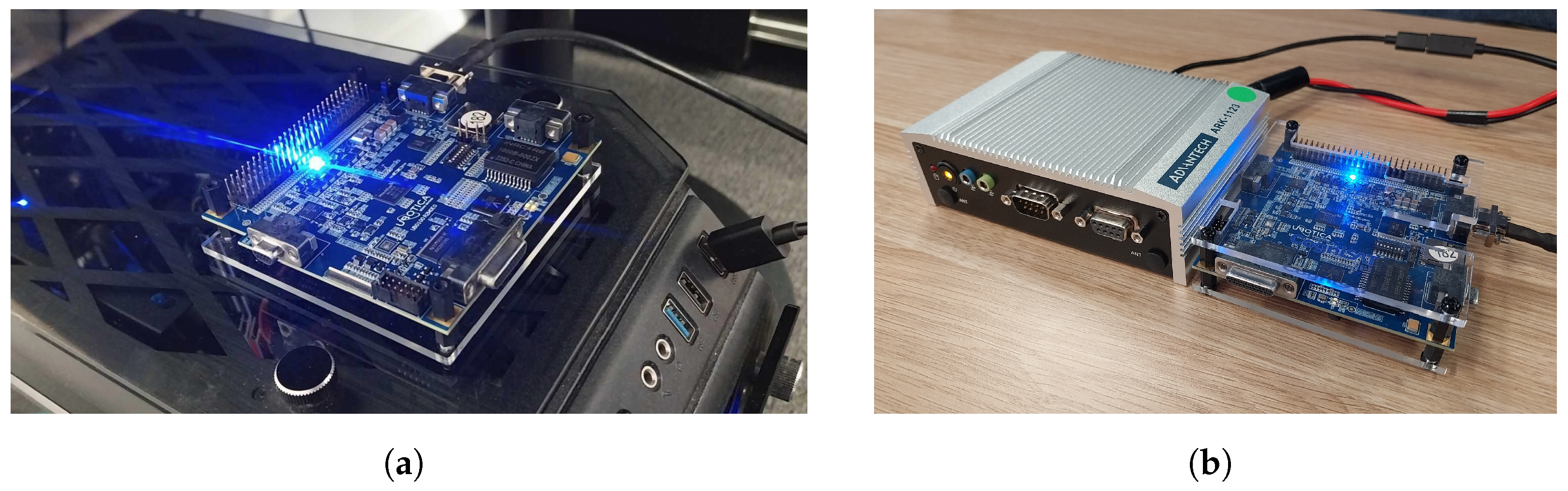
To solve Problem 2 in Section 3.3.2, we built and ran an ONNX Runtime (ORT) [81] on a standard Linux desktop connected to a Ubotica CogniSAT-XE1 (“XE1” for short) [13] via USB (see Figure 5a):
- The XE1 is a low-power edge processing device designed for SmallSat and CubeSat missions. It features the Intel Myriad 2 VPU and its main purpose is to accelerate machine learning inference.
- ORT was selected since it only requires ≈ 18.1 MB (version 1.15) of disk space and supports a wide range of operating systems and programming languages.
Prior to deploying onto the satellite in the pre-deployment model training phase (see Figure 2), the model was converted to the ONNX format, which was then used to generate training artefacts (i.e., training, evaluation and optimiser ONNX models, as well as checkpoint states). As Figure 6 shows, these training artefacts were then deployed onto the satellite for executing the TTA algorithms on CPU. For emulating the CPU aboard the HyperScout-2 hyperspectral imager, an Advantech ARK-1123L [82] embedded computer was used. Post-deployment model testing was performed on (i) the XE1 connected to the Linux desktop (Figure 5a) and (ii) the XE1 connected to the ARK-1123L (Figure 5b).
Figure 6.
Training artefacts and target data are used in online adaptation, which is executed on the CPU of an embedded computer aboard the satellite (in orbit). Inference is then executed on a VPU-based device.
Figure 5.
Hardware platforms used in this study. (a) Cloud detectors are trained on a Linux desktop before they are deployed onto the Ubotica CogniSAT-XE1. (b) Post-deployment, the Advantech ARK-1123L and Ubotica CogniSAT-XE1 perform TTA and cloud detection, respectively.
One well-known TTA approach [69,71,83,84] is to update the BN layers of a deep network, which, in our case, is the source cloud detector , in an unsupervised manner, using, in our case, the unlabelled target dataset . The role of BN is to normalise the intermediate outputs of each layer to zero mean and unit variance. However, this normalisation effect breaks when the source and target distributions significantly differ. As described in Algorithm 2, TTA is executed by the function but only when a batch of target samples is collected and reaches a certain (predefined) size . This function is implemented using dynamic unsupervised adaptation (DUA) [71] (see Section 6.2.1) and, alternatively, test-time entropy minimisation (Tent) [69] (see Section 6.2.2), since both methods are efficient in terms of computing power (i.e., they do not rely on supervision or processing of source data) and memory usage (i.e., they do not rely on source data or a large batch of target data to be saved on the compute hardware of the satellite).
| Algorithm 2 TTA algorithm |
▹ Copy source weights to target weights ▹ Initialise current batch for to do if then end if end for |
6.2.1. DUA
DUA [71] updates the running means and running variances of the BN layers of . More concretely, let us define , , and m as the running means, running variances and momentum of an arbitrary BN layer of , respectively. Furthermore, let and be the mean and variance of the batch . DUA first updates the momentum of the BN layer,
where is the predefined momentum decay parameter and defines the lower bound of the momentum. Then, the running mean and running variance are updated as
The main idea of DUA is to gradually decay the momentum m, because a fixed momentum can demonstrably destabilise or slow down the convergence of the adaptation process [71].
The computational complexity of DUA is dominated by the computation of and in Equations (8) and (), which requires expectation operations for each BN layer. Thus, the computational complexity of DUA is expectation operations, where is the number of BN layers.
6.2.2. Tent
Similar to DUA [71], Tent [69] also updates the the BN layers of but with one minor difference—the affine transformation parameters are also updated. Recall and are the running mean and running variance of an arbitrary BN layer of . We further denote and as the affine transformation parameters of the BN layer. Given batch , Tent [69] first estimates the Shannon entropy loss:
where C is total number of classes, is the prediction of , and is the predicted probability of of class c. Tent comprises as many iterations as the number of samples in a batch, where each iteration consists of a forward pass and a backward pass. During a forward pass, the normalisation statistics for each BN layer are estimated/updated. A backward pass follows the prediction for the current batch. During a backward pass, the transformation parameters are updated, so the updated parameters only affect the next batch. In summary, each BN layer is updated in terms of
In contrast to DUA [71], Tent [69] uses a fixed momentum, and the normalisation statistics , are recalculated from scratch on the target data.
Excluding forward propagation and backward propagation, the computational complexity of Tent in one epoch, like that of DUA, is expectation operations, where is the number of BN layers.
7. Evaluation Platforms and Metrics
In order to execute a cloud detector on the XE1 (introduced in Section 6.2), the model format must be converted to the Ubotica neural network (UNN) format. This conversion involves 3 steps:
- Export the model to the ONNX format.
- Convert the generated ONNX files to the OpenVINO Intermediate Representation format.
- Convert the OpenVINO Intermediate Representation to the Ubotica Neural Network (UNN) format.
Note that Step 2 also quantises from FP32 to FP16, which is required to run inference on the Intel Myriad 2 VPU. The inference performance of on a dataset is evaluated based on two metrics:
- Accuracy (ACC) of ,where is the indicator function, and . The higher the test accuracy means the higher predicts the correct class label. This helps in increasing the quality of each prediction, especially in challenging situations, e.g., clouds on ice or clouds on salt-lake.
- False positive (FP) rate of ,The lower the FP rate means the less incorrectly predicts non-cloudy data cubes as cloudy, which helps avoid discarding clear-sky data cubes.
False negatives refer to the cases where cloudy images are misclassified as non-cloudy, resulting in downlinking cloudy images. As false negatives do not directly lead to data loss, whereas false positives do, false negatives are not as disruptive as false positives. Nevertheless, for the experiments on Ubotica CogniSAT-XE1 reported in Section 8.3, false negative rates are available through the confusion matrices in Appendix B.
The inference performance of on source and target datasets (Section 4.3) can be evaluated by substituting with and respectively. In principle, the inference performance is to be evaluated on the XE1 since it is the target device of interest. However, we found based on preliminary testing that there were minute differences in ACC and FP rate when we evaluated with FP32 weights on a Linux desktop and FP16 weights on the XE1.
8. Results
In this section, we first empirically establish the presence of a nontrivial domain gap in the multispectral cloud detection task (Section 8.1). Then, we evaluate the performance of the proposed algorithms for offline and online domain adaptation (Section 8.2).
8.1. Domain Gap in Multispectral Data
We trained the cloud detector in Table 4 on the source dataset and evaluated their performance on the target dataset, without domain adaptation. For cloud detectors trained on three bands, we selected (i) bands 1, 2, 8a of Sentinel-2 and (ii) bands 1, 2, 5 of Landsat 9. Otherwise, we used the eight shared bands of Sentinel-2 and Landsat 9. The different combinations of model settings are indicated by the naming convention
where
- ARCH is the architecture of either CloudScout or ResNet50,
- NUMBANDS is either 3 or 8,
- SOURCE is either S2 for Sentinel-2 or L9 for Landsat 9.
For example, CloudScout-8-L9 refers to training the CloudScout architecture with eight bands on Landsat 9 defined as the source domain. The different datasets used to evaluate the source cloud detectors are indicated by the naming convention:
where
- SAT is either S2 for Sentinel-2 or L9 for Landsat 9,
- SET is either TRAIN for training set or TEST for testing set.
For example, S2-TEST means the testing set consisting of Sentinel-2 data. Note that the training and testing sets have ground-truth labels obtained by applying a 70% threshold to the cloud masks. The major findings that can be observed from the results in Table 5 are as follows:
- The domain gap is more prominent in cloud detectors trained on eight bands compared to their three-band counterparts; observe the difference in performance between CloudScout-3-S2 (ACC/FP of 66.40%/0.80%) and CloudScout-8-S2 (ACC/FP of 52.00%/ 48.00%) evaluated on the L9-TEST.
- The domain gap appears to be smaller in ResNet50 than CloudScout; observe the difference in performance between CloudScout-3-S2 (ACC/FP of 66.40%/0.80%) and ResNet50-3-S2 (ACC/FP of 90.80%/1.60%) evaluated on L9-TEST.
- Overall, the effects of the domain gap are significant, since it prevents machine learning models from performing as required by EO mission standards, e.g., CloudScout [5] requires a minimum ACC of 85% and maximum FP of 1.2%.
The results were obtained by training and evaluating cloud detectors with FP32 weights on a Linux desktop since quantising the weights to FP16 was found to have negligible effects on performance when evaluated on the XE1. The results also confirm the necessity of domain adaptation.
Table 5.
Model performance of cloud detectors without domain adaptation. GAP is the absolute difference in performance between the testing sets of Sentinel-2 and Landsat 9. The red text and green text show negative and positive effects on performance, respectively.
8.2. Ablation Studies
We present ablation studies in order to examine the approaches we employed for offline and online adaptation more carefully. These studies were also performed on cloud detectors with FP32 weights on a Linux desktop.
8.2.1. Bandwidth-Efficient SDA
The FISH Mask [80] was applied to the source cloud detectors (Section 8.1) with varying mask sparsity levels and optimisation conducted over a fixed number of 300 epochs. The entire training set of the target dataset was used to estimate the Fisher information of each weight.
We found that only a small subset of weights were required to achieve similar model performance as updating 100% of the weights. Specifically, Figure 7a suggests that for CloudScout models, only 25% of the total weights need to be updated, whereas Figure 7b suggests that for ResNet50 models, only 1% are needed. While a higher mask sparsity level generally leads to a higher adaptation performance, CloudScout-3-S2 and CloudScout-8-L9 give us two examples of how updating 25% of the weights provides better adaptation than updating all the weights (see Figure 7a). These counter-intuitive results can be explained through the number of variables in optimisation problem (6): more optimisation variables could require more epochs to converge to a good local solution, so for the same number of epochs, fewer optimisation variables could lead to a better local solution.
Figure 7.
Effects of FISH Mask on cloud detectors for different mask sparsity levels. SOURCE ONLY refers to training cloud detectors only on source data. FC ONLY means that only the weights in the FC layers were updated.
The results indicate the usefulness of the FISH Mask in alleviating the uplink restrictions on model size, although this applies only to offline adaptation (Section 3.3.1), which assumes a labelled target dataset.
8.2.2. TTA on Satellite Hardware: DUA
Of the two proposed TTA methods, DUA [71] was first applied to CloudScout-3-S2 and evaluated for different numbers of samples used for adaptation. The effect of data augmentation on DUA was also evaluated by generating batches of augmented samples—one batch from each test sample—and using the generated batches for adaptation.
Number of samples: Figure 8a shows the effects of varying the number of samples used to update CloudScout-3-S2 to Landsat 9. We found that ACC saturates at 16 samples; this trend is consistent with Mirza et al.’s observations [71]. The optimal number of samples corresponds to the point of diminishing returns for ACC, because past this point, the FP rate continues to rise. The ordering of the incoming samples holds little significance as it has negligible impact on model performance; this again confirms Mirza et al.’s observations [71]. These results demonstrate the memory-efficiency of DUA, as peak performance is achievable using a small amount of unlabelled target data. This efficiency can be attributed to these key factors:
Figure 8.
Effects of DUA on CloudScout-3-S2. SOURCE ONLY refers to CloudScout-3-S2 trained only on source data. Error bars represent standard deviations over 10 runs with different random seeds. (a) Model performance for different numbers of test samples without data augmentation. (b) Model performance for different augmentation batch sizes and a fixed number of 16 batches (one batch for each test sample).
- DUA utilises models pretrained on source-domain data. This pre-training helps a model learn general features that are often shared across different domains. As a result, the model requires only minor adjustments to adapt to the target domain, avoiding the need for a large amount of new data.
- The statistics of the source and target domain, such as the mean and variance, may exhibit a high degree of similarity. When these statistics are closely aligned, a model is efficiently transferable across domains, i.e., the model parameters can be adapted to a new domain using few new samples.
Data augmentations: Each sample is augmented by random horizontal flipping, cropping and rotation. The term “augmentation batch size” refers to the number of augmented samples in a batch. Figure 8b shows the effects of varying the augmentation batch size. Contrary to [71], we found that increasing the augmentation batch size does not provide further improvements in model performance. This is good news because it eliminates the need for data augmentation and thus reduces the time and computational efforts of DUA to perform adaptation.
8.2.3. TTA on Satellite Hardware: Tent
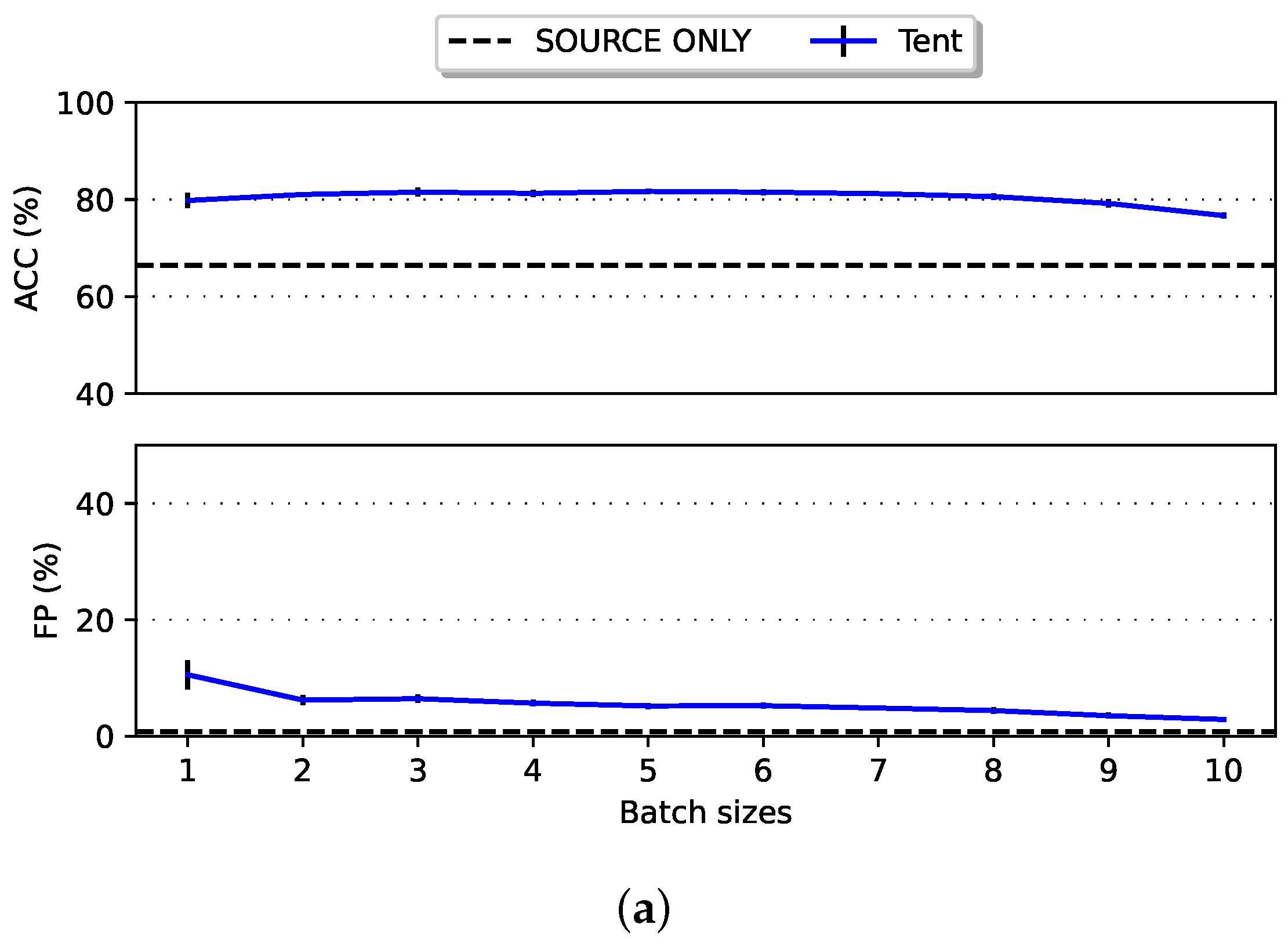
Next, Tent [69] was applied to CloudScout-3-S2 and evaluated for different batch sizes and numbers of epochs.
Batch size: Figure 9a shows the effects of varying the batch size. We found that a batch size of 8 gives the best balance in performance in terms of increasing ACC and decreasing FP. Balancing batch size is critical for achieving optimal performance with Tent due to the following reasons:
- Small batches provide noisier gradient estimates because each batch is less representative of the overall data distribution. This noise in the gradient estimates can lead to more erratic updates to the model weights, causing oscillations in the loss curve, where the loss may fluctuate rather than decrease smoothly. Consequently, this instability in the training process can be observed to have produced spread in the ACC and FP.
- Larger batches provide more stable and accurate gradient estimates, which can lead to a smoother path to convergence and fewer FPs. However, as the results show, increasing the batch size too much can degrade the ACC on data aligned with the source distribution; this performance degradation is known as error accumulation and catastrophic forgetting in the literature [43].
Similar to DUA, Tent is also memory-efficient since it does not need to wait for a large batch of target data.
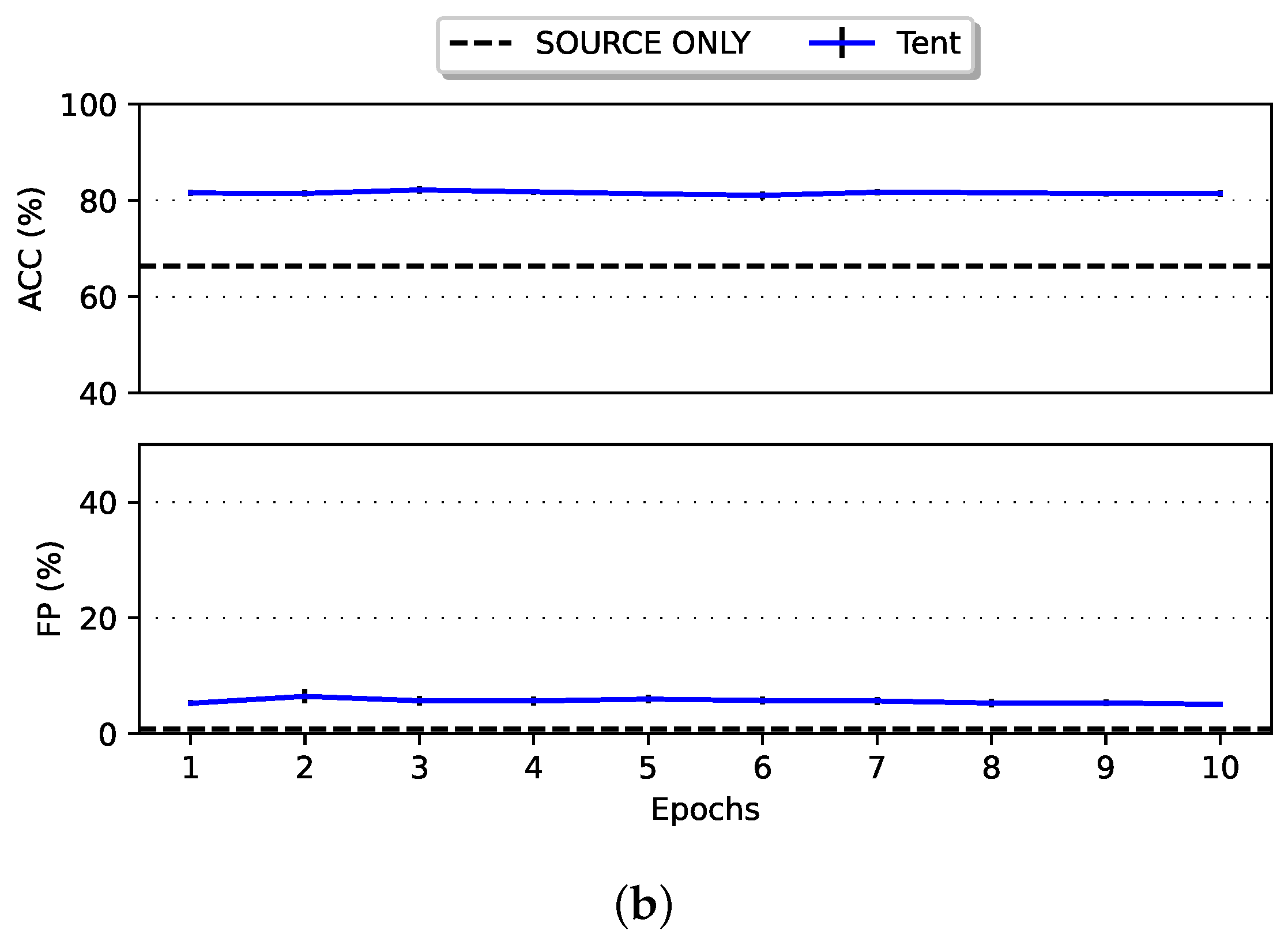
Number of epochs: A total of 250 test-time samples were processed every epoch. Figure 9b shows no further improvements in performance beyond 1 epoch. This is good news because it eliminates the need to cycle through the same samples more than once and thus, reduces the time and computational efforts of Tent to perform adaptation to its maximum ability.
Figure 9.
Effects of Tent on CloudScout-3-S2. SOURCE ONLY refers to CloudScout-3-S2 trained only on source data. Error bars represent standard deviations over 10 runs with different random seeds. (a) Model performance for different batch sizes and a fixed number of 1 epoch. (b) Model performance for different numbers of epochs and a fixed batch size of 8.
Lastly, we applied both TTA methods—DUA and Tent—on the remaining source cloud detectors (Section 8.1). As shown in Figure 10, Tent outperforms DUA in most cases but only by a slight margin. This was expected since DUA only updates the normalisation statistics in the BN layers. However, Tent requires more computational resources since it needs to perform backpropagation to update the affine transformation parameters.
Figure 10.
Effects of DUA and Tent on the cloud detectors in Table 5. SOURCE ONLY refers to training cloud detectors only on source data. Error bars represent standard deviations over 10 runs with different random seeds. (a) Model performance of the cloud detectors in Table 5a. (b) Model performance of the cloud detectors in Table 5b.
8.3. Performance on Ubotica CogniSAT-XE1
Once the source and target cloud detectors have been obtained, we executed them on the Ubotica CogniSAT-XE1 [13] and evaluated their performance. The effects of domain adaptation by the proposed methods are visualised in Figure 11. Table 6a shows the ACC and FP results for the Sentinel-2-trained cloud detectors before and after domain adaptation, as well as the memory footprints and inference times of the cloud detectors. Table 6b shows the same types of results as Table 6a but for Landsat-9-trained cloud detectors. Appendix B supplements Table 6 with confusion matrices that facilitate the calculation of additional metrics such as precision, recall and F1-score. Table 7 zooms in on the execution times of the TTA methods for the Sentinel-2-trained cloud detectors, as measured on the Advantech ARK-1123L [82] embedded computer, where 16 test-time samples were used for DUA and a batch size of 1 was used for Tent.
Figure 11.
Visualisation of CloudScout-3-S2 performing cloud detection on multispectral data from Landsat 9, where the subcaptions specify the domain adaptation methods for which the subsequent statements are valid. (Top) Cloudy images (a–c) are misclassified as not cloudy before domain adaptation but are correctly classified as cloudy after domain adaptation. (Bottom) Non-cloudy images (d–f) are misclassifed as cloudy before domain adaptation but are correctly classified as not cloudy after domain adaptation. (a) FISH Mask, DUA and Tent. (b) Fish Mask and DUA. (c) Fish Mask and Tent. (d) FISH Mask. (e) DUA. (f) Tent.
Table 6.
Model performance of the source cloud detectors in Table 5 with domain adaptation (FISH Mask, DUA and Tent) and without domain adaptation (SOURCE ONLY) on the Ubotica CogniSAT-XE1. Red text and green text show the negative and positive effects on performance, respectively. Comparison also includes (i) memory footprint (in MB using FP16 weights), and (ii) inference time (in ms per sample).
Table 7.
Execution time (s) of TTA methods for source cloud detectors in Table 5a on the Advantech ARK-1123L embedded computer. For Tent, the embedded computer ran out of memory for any batch size larger than 1.
Our results confirm the following:
- For offline adaptation, we can solve Problem 1 in Section 3.3.1 by employing the FISH Mask and, thereby, enabling more sophisticated models to be deployed and updated remotely through the thin uplink channel. As expected, we found that this adaptation approach outperforms the TTA approaches by a large margin. Note that CloudScout and ResNet50 models with a mask sparsity level of 25% and 1%, respectively, were only evaluated here.
- For online adaptation, while Tent has a slight performance advantage in ACC over DUA, the advantage does not extend to FP rate, and furthermore, Tent is 60–100% more computationally expensive than DUA. Nevertheless, both TTA methods are evidently viable on satellite-borne edge compute hardware.
Other findings from our results are as follows:
- Quantising the weights from FP32 to FP16 had negligible effects on model performance, as well as the added benefit of reducing the memory footprint by two-fold.
- ResNet50 models had a faster inference time (per sample) than CloudScout models, which is surprising since they are ≈18× larger in size.
9. Discussion
In this section, we discuss some limitations of the experimentation and proposed domain adaptation methods, as well as some potential extensions of the methods.
9.1. Preprocessing
The impact of data preprocessing on the domain gap and domain adaptation has not been explored. Relevant to our study, in aspects of preprocessing, are multiple projects “harmonising” Landsat and Sentinel-2 EO data into a single analysis-ready “virtual constellation” dataset [76,77]. Harmonisation involves applying a range of geometric, atmospheric, spectral and directional effect correction operations to data products from multiple sources to create a time-series dataset suitable for continuous Earth surface monitoring [76,77]. These harmonisation operations can potentially be used to provide training data for onboard cloud detectors, with the benefit of reducing the domain gap better than the preprocessing steps described in Section 4, but this hypothesis has yet to be systematically explored.
9.2. Experimentation
As shown in Figure 5, three main hardware platforms were involved in this study:
- A Ubotica CogniSAT-XE1 (XE1) [13]: In an EO mission, this is responsible for model inferencing. The experimental results in Table 6 were obtained on this platform.
- An Advantech ARK-1123L [82]: In an EO mission, this is responsible for TTA. The experimental results in Table 7 were obtained on this platform.
- A Linux desktop: In an EO mission, this is limited to model training, but since there were minute differences in ACC and FP rate between a desktop-hosted version and an XE1-hosted version of the same model, the experimental results on ACC and FP rate in Figure 7, Figure 8, Figure 9, Figure 10 and Figure 11 were obtained on a Linux desktop. Realism was compromised in this setting, but the domain adaptation methods were evaluated and compared on an equal footing.
No UDA schemes were included in our experimentation because once target-domain data are downlinked, performing UDA using the unlabelled target data and subsequently updating the satellite-borne model partially (rather than fully) using FISH Mask predictably produces lacklustre results.
9.3. Performance of TTA
Our results in Section 8.3 show that even though DUA and Tent can reduce the domain gap, their effectiveness fails to match that of SDA using FISH Mask; compare the performances of DUA and Tent in Figure 10 to the upper-bound performance of FISH Mask (applied to source cloud detectors at a mask sparsity level of 100%) in Figure 7a. At this stage, the TTA methods may not be effective enough to be recommended for online adaptation (i.e., onboard updating of machine learning models). Updating other layers of the model, in addition to the batch normalisation layers, in an unsupervised manner could enhance the performance of TTA methods, but how to perform this update remains an open problem.
9.4. Extension to Hyperspectral Applications
Although the work reported so far was conducted on multispectral rather than hyperspectral data, the number of spectral bands (dimensionality) is not a limiting factor for either CloudScout or the domain adaptation methods. For example, adding one spectral band requires adding one input channel to the first convolutional layer of CloudScout, although more convolutional layers and weights per layer may need to be added to maintain the same performance. The proposed domain adaptation methods will work on any CNN architecture and are independent of the number of bands used. The preceding statements, however, are not meant to downplay the challenges associated with the infamous “curse of dimensionality” or Hughes phenomenon [85]. Furthermore, as energy is spread out over more bands, the signal-to-noise ratio (SNR) per band suffers [86]. Depending on the sensor characteristics and mission requirements, denoising (i.e., noise reduction) may be a necessary preprocessing step before cloud detection [15]. In summary, enhancing the proposed methods to process hyperspectral data requires a straightforward albeit nontrivial extension of said methods. Nevertheless, representative or real-world performance of the enhanced/extended methods on hyperspectral data can only be evaluated using a more capable VPU than what is available for our current investigation.
9.5. Adapting to Constraints
Real-world scenarios are rife with challenging operational constraints, which EO missions need to adapt to in order to maximise return on investment. These constraints include the following [87]:
- Energy constraint: Onboard machine learning can be computationally intensive and thus power-hungry, but EO satellites typically rely on photovoltaics and battery storage for energy supply. To avoid the risk of unrecoverable energy depletion, it is crucial to monitor the state of charge (SoC) of the battery and only perform power-hungry computation such as onboard updating of machine learning models when the SoC is at a sustainable level.
- Downlink bandwidth constraint: The time during which a satellite and a ground station are within communication range of each other, allowing the satellite to downlink its data to the ground station, is known as the communication window. The size of the communication window, the capacity of the communication channel (e.g., RF, optical) and environmental effects (e.g., multipath, atmospheric turbulence, space weather) determine the amount of data that can be downlinked; if this amount is less than how much the satellite needs to downlink, then the satellite should selectively downlink the data that improve domain adaptation the most. The detail of the selection strategy is a topic of our ongoing research.
- Uplink bandwidth constraint: The fact that uplink bandwidth is more limited than downlink bandwidth, as mentioned in Section 3.3.1, incentivises further conservation of uplink bandwidth by the bandwidth-efficient SDA method proposed in Section 6.1. A naive application of the proposed SDA method could see the ground station (i) executing the FISH Mask algorithm on the labelled target dataset to update the model weights and (ii) uploading the updated model weights defined by Equation (6) to the EO satellite during every communication window. However, valuable uplink bandwidth can be conserved if the FISH Mask algorithm is only executed on whenever the sum of losses exceeds a certain threshold. How this threshold can be set for a desired trade-off between domain gap and bandwidth usage is another topic of our ongoing research.
In summary, the proposed domain adaptation methods can be extended to account for the preceding constraints.
10. Conclusions and Future Study
We showed the existence of the domain gap when training a real-world CNN-based multispectral cloud detector on data from one EO mission and evaluating it on data from another mission. To address the domain gap, we proposed domain adaptation tasks framed in two different settings of an EO mission: (i) offline adaptation and (ii) online adaptation. For offline adaptation, our results show that only a small fraction of weights need to be updated (in a supervised manner) without noticeable impacts on performance. This enables more sophisticated and robust models to be deployed and remotely updated. Whereas for online adaptation, our results show the viability of test-time adaptation algorithms on space hardware. This enables us to directly update models onboard in an unsupervised manner. The collection of results and insights reported in this paper should provide a timely reference for EO mission planners who are increasingly interested in satellite-borne machine learning. Our source code is publicly available at: https://github.com/andrewpatrickdu/domain-adaptation-cloud-detection (accessed on 11 September 2024).
For future work, we plan on: (i) investigating other means of performing online adaptation that can satisfy the requirements in accordance with EO mission standards and (ii) showing how our work can be extended to hyperspectral EO applications by simply increasing the number of spectral bands for the cloud detection and domain adaptation algorithms. However, representative or real-world performance of the enhanced/extended algorithms on hyperspectral data cubes can only be evaluated using a significantly more capable compute payload than what is available for our current investigation.
Author Contributions
Conceptualisation, A.D., A.-D.D. and T.-J.C.; data curation, A.D.; formal analysis, A.D.; funding acquisition, T.-J.C.; investigation, A.D. and Y.W.L.; methodology, A.D., A.-D.D., Y.W.L. and T.-J.C.; project administration, T.-J.C.; software, A.D.; supervision, A.-D.D., Y.W.L. and T.-J.C.; validation, A.D.; visualisation, A.D.; writing—original draft, A.D.; writing—review and editing, A.D., A.-D.D., Y.W.L. and T.-J.C. All authors have read and agreed to the published version of the manuscript.
Funding
This research was partially funded by SmartSat CRC, Research Program 2: Advanced Satellite Systems, Sensors and Intelligence. Tat-Jun Chin is SmartSat CRC Professorial Chair of Sentient Satellites.
Data Availability Statement
Datasets Sentinel-2-Cloud-Mask-Catalogue and Landsat-9-Level-1 are available at https://universityofadelaide.box.com/s/f60mhnbv8tbysgxrv9dps3v6zoazg0ic (accessed on 11 September 2024).
Conflicts of Interest
The authors declare no conflict of interest.
Acronyms
The following acronyms are used in this manuscript. Note common nouns are in lower case, whereas names are capitalised.
| ACC | accuracy |
| BN | batch normalisation |
| CNN | convolutional neural network |
| CPGA | contrastive prototype generation and adaptation |
| CPU | central processing unit |
| DANN | domain-adversarial neural network |
| DNN | deep neural network |
| DUA | dynamic unsupervised adaptation |
| EO | Earth observation |
| FISH | Fisher-Induced Sparse uncHanging |
| Fmask | Function of mask |
| FP | false positive |
| GPU | graphics processing unit |
| NDCI | normalised difference cloud index |
| ReLU | rectified linear unit |
| SDA | supervised domain adaptation |
| SNR | signal-to-noise ratio |
| SoC | state of charge |
| SSDA | semi-supervised domain adaptation |
| Tent | test-time entropy minimisation |
| TOA | top-of-atmosphere |
| TTA | test-time adaptation |
| UDA | unsupervised domain adaptation |
| UNN | Ubotica neural network |
| VPU | vision processing unit |
Appendix A. Additional Details on Sensor Variations
The information here continues from Section 1.1 on the different aspects sensors (even from the same build) can differ in:
- Spectral band and spectral response: A spectral band is defined by (i) its wavelength range and (ii) the spectral response over this range. Spectral response is photocurrent level per incident light level, measured in ampere per watt, as a function of wavelength [88]. Wavelength ranges are typically selected to maximise object-to-background contrast; for example, Sentinel-2 uses a narrow band at 865 nm because iron-oxide soil exhibits an absorption band in the 850–900 nm region [11,89]. However, imagers configured to observe the same wavelength ranges can exhibit different spectral responses.
- Spatial resolution: This is a measure of the smallest angular or linear separation between two objects that can be resolved by the imager [89]. Equivalently, the spatial resolution is the area on the ground each pixel occupies. Spatial resolution can vary from one spectral band to another. Furthermore, imagers with the same spectral bands can provide different spatial resolutions.
- SNR: For a spectral band, the SNR is the mean of the measured radiances divided by their standard deviation [90]. Among the factors that determine the SNR are the sources of shot noise and thermal noise in the photodetector–preamplifier circuit [88]. SNR can vary from one spectral band to another. Imagers with the same spectral bands can have different SNRs.
- Calibration error and instrument drift: Imagers with the same spectral bands can be subject to different calibration errors and instrument drift characteristics. For example, brightness temperature data obtained from different geostationary meteorological satellites have been observed to vary for the same/similar scenes not only due to differences in the spectral characteristics but also due to calibration errors and sensor drift among these satellites [91].
Appendix B. Additional Results on Ubotica CogniSAT-XE1
In addition to the values of ACC and FP rate in Table 6, the confusion matrices in Table A1, Table A2, Table A3, Table A4, Table A5, Table A6, Table A7 and Table A8 below, also obtained on the Ubotica CogniSAT-XE1, facilitate the calculation of precision, recall and F1-score. For example, in Table A1, FISH Mask has
- precision ,
- recall (note false negative rate = 1 − recall),
- F1-score .
Table A1.
Confusion matrices supplementing Table 6a for CloudScout-3-S2 evaluated on L9-TEST, without domain adaptation (SOURCE ONLY) and with domain adaptation (FISH Mask, DUA and Tent).
Table A2.
Confusion matrices supplementing Table 6a for CloudScout-8-S2 evaluated on L9-TEST, without domain adaptation (SOURCE ONLY) and with domain adaptation (FISH Mask, DUA and Tent).
Table A3.
Confusion matrices supplementing Table 6a for ResNet50-3-S2 evaluated on L9-TEST, without domain adaptation (SOURCE ONLY) and with domain adaptation (FISH Mask, DUA and Tent).
Table A4.
Confusion matrices supplementing Table 6a for ResNet50-8-S2 evaluated on L9-TEST, without domain adaptation (SOURCE ONLY) and with domain adaptation (FISH Mask, DUA and Tent).
Table A5.
Confusion matrices supplementing Table 6b for CloudScout-3-L9 evaluated on S2-TEST, without domain adaptation (SOURCE ONLY) and with domain adaptation (FISH Mask, DUA and Tent).
Table A6.
Confusion matrices supplementing Table 6b for CloudScout-8-L9 evaluated on S2-TEST, without domain adaptation (SOURCE ONLY) and with domain adaptation (FISH Mask, DUA and Tent).
Table A7.
Confusion matrices supplementing Table 6b for ResNet50-3-L9 evaluated on S2-TEST, without domain adaptation (SOURCE ONLY) and with domain adaptation (FISH Mask, DUA and Tent).
Table A8.
Confusion matrices supplementing Table 6b for ResNet50-8-L9 evaluated on S2-TEST, without domain adaptation (SOURCE ONLY) and with domain adaptation (FISH Mask, DUA and Tent).
References
- Euroconsult. Earth Observation Satellites Set to Triple over the Next Decade. 2024. Available online: https://www.euroconsult-ec.com/press-release/earth-observation-satellites-set-to-triple-over-the-next-decade/ (accessed on 11 September 2024).
- European Space Agency. PhiSat-1 Nanosatellite Mission. In Satellite Missions Catalogue, eoPortal; European Space Agency: Paris, France, 2020. [Google Scholar]
- Esposito, M.; Conticello, S.S.; Pastena, M.; Domínguez, B.C. In-orbit demonstration of artificial intelligence applied to hyperspectral and thermal sensing from space. In Proceedings of the CubeSats and SmallSats for Remote Sensing III, San Diego, CA, USA, 11–12 August 2019; Pagano, T.S., Norton, C.D., Babu, S.R., Eds.; International Society for Optics and Photonics. SPIE: Philadelphia, PA, USA, 2019; Volume 11131, p. 111310C. [Google Scholar] [CrossRef] [Scilit]
- Deniz, O.; Vallez, N.; Espinosa-Aranda, J.L.; Rico-Saavedra, J.M.; Parra-Patino, J.; Bueno, G.; Moloney, D.; Dehghani, A.; Dunne, A.; Pagani, A.; et al. Eyes of Things. Sensors 2017, 17, 1173. [Google Scholar] [CrossRef] [Scilit] [PubMed]
- Giuffrida, G.; Diana, L.; de Gioia, F.; Benelli, G.; Meoni, G.; Donati, M.; Fanucci, L. CloudScout: A Deep Neural Network for On-Board Cloud Detection on Hyperspectral Images. Remote Sens. 2020, 12, 2205. [Google Scholar] [CrossRef] [Scilit]
- Giuffrida, G.; Fanucci, L.; Meoni, G.; Batič, M.; Buckley, L.; Dunne, A.; van Dijk, C.; Esposito, M.; Hefele, J.; Vercruyssen, N.; et al. The Φ-Sat-1 Mission: The First On-Board Deep Neural Network Demonstrator for Satellite Earth Observation. IEEE Trans. Geosci. Remote Sens. 2022, 60, 5517414. [Google Scholar] [CrossRef] [Scilit]
- ESA. S2 Mission: Overview of Sentinel-2 Mission. SentiWiki. 2021. Available online: https://sentiwiki.copernicus.eu/web/s2-mission (accessed on 27 August 2024).
- Kouw, W.M.; Loog, M. An introduction to domain adaptation and transfer learning. arXiv 2019, arXiv:1812.11806. [Google Scholar] [CrossRef] [Scilit]
- ISO 24585-1:2023; Graphic Technology—Multispectral Imaging Measurement and Colorimetric Computation for Graphic Arts and Industrial Application—Part 1: Parameters and Measurement Methods. ISO: Geneva, Switzerland, 2023.
- Hagen, N.A.; Kudenov, M.W. Review of snapshot spectral imaging technologies. Opt. Eng. 2013, 52, 090901. [Google Scholar] [CrossRef] [Scilit]
- European Space Agency. Sentinel-2 User Handbook; Issue 1 Rev 2; European Space Agency: Paris, France, 2015. [Google Scholar]
- Ma, D.; Rehman, T.U.; Zhang, L.; Maki, H.; Tuinstra, M.R.; Jin, J. Modeling of Environmental Impacts on Aerial Hyperspectral Images for Corn Plant Phenotyping. Remote Sens. 2021, 13, 2520. [Google Scholar] [CrossRef] [Scilit]
- Ubotica. CogniSAT-XE1: AI and Computer Vision Edge Computing Platform Overview. 2023. Available online: https://ubotica.com/ubotica-cognisat-xe1/ (accessed on 7 February 2023).
- Jeppesen, J.H.; Jacobsen, R.H.; Inceoglu, F.; Toftegaard, T.S. A cloud detection algorithm for satellite imagery based on deep learning. Remote Sens. Environ. 2019, 229, 247–259. [Google Scholar] [CrossRef] [Scilit]
- Li, H.; Zheng, H.; Han, C.; Wang, H.; Miao, M. Onboard Spectral and Spatial Cloud Detection for Hyperspectral Remote Sensing Images. Remote Sens. 2018, 10, 152. [Google Scholar] [CrossRef] [Scilit]
- Li, X.; Wang, L.; Cheng, Q.; Wu, P.; Gan, W.; Fang, L. Cloud removal in remote sensing images using nonnegative matrix factorization and error correction. ISPRS J. Photogramm. Remote Sens. 2019, 148, 103–113. [Google Scholar] [CrossRef] [Scilit]
- Meraner, A.; Ebel, P.; Zhu, X.X.; Schmitt, M. Cloud removal in Sentinel-2 imagery using a deep residual neural network and SAR-optical data fusion. ISPRS J. Photogramm. Remote Sens. 2020, 166, 333–346. [Google Scholar] [CrossRef] [Scilit]
- Zi, Y.; Xie, F.; Zhang, N.; Jiang, Z.; Zhu, W.; Zhang, H. Thin Cloud Removal for Multispectral Remote Sensing Images Using Convolutional Neural Networks Combined with an Imaging Model. IEEE J. Sel. Topics Appl. Earth Observ. Remote Sens. 2021, 14, 3811–3823. [Google Scholar] [CrossRef] [Scilit]
- Sinergise Laboratory. Cloud Masks. In Sentinel Hub User Guide; Sinergise Laboratory: Ljubljana, Slovenia, 2021. [Google Scholar]
- Marshak, A.; Knyazikhin, Y.; Davis, A.B.; Wiscombe, W.J.; Pilewskie, P. Cloud-vegetation interaction: Use of normalized difference cloud index for estimation of cloud optical thickness. Geophys. Res. Lett. 2000, 27, 1695–1698. [Google Scholar] [CrossRef] [Scilit]
- Zhu, Z.; Woodcock, C.E. Object-based cloud and cloud shadow detection in Landsat imagery. Remote Sens. Environ. 2012, 118, 83–94. [Google Scholar] [CrossRef] [Scilit]
- Tang, B.H.; Shrestha, B.; Li, Z.L.; Liu, G.; Ouyang, H.; Gurung, D.R.; Giriraj, A.; Aung, K.S. Determination of snow cover from MODIS data for the Tibetan Plateau region. Int. J. Appl. Earth Obs. Geoinf. 2013, 21, 356–365. [Google Scholar] [CrossRef] [Scilit]
- Li, Z.; Shen, H.; Weng, Q.; Zhang, Y.; Dou, P.; Zhang, L. Cloud and cloud shadow detection for optical satellite imagery: Features, algorithms, validation, and prospects. ISPRS J. Photogramm. Remote Sens. 2022, 188, 89–108. [Google Scholar] [CrossRef] [Scilit]
- Mahajan, S.; Fataniya, B. Cloud detection methodologies: Variants and development—A review. Complex Intell. Syst. 2020, 6, 251–261. [Google Scholar] [CrossRef] [Scilit]
- López-Puigdollers, D.; Mateo-García, G.; Gómez-Chova, L. Benchmarking Deep Learning Models for Cloud Detection in Landsat-8 and Sentinel-2 Images. Remote Sens. 2021, 13, 992. [Google Scholar] [CrossRef] [Scilit]
- Liu, Y.; Wang, W.; Li, Q.; Min, M.; Yao, Z. DCNet: A Deformable Convolutional Cloud Detection Network for Remote Sensing Imagery. IEEE Geosci. Remote Sens. Lett. 2021, 19, 8013305. [Google Scholar] [CrossRef] [Scilit]
- Li, S.; Song, W.; Fang, L.; Chen, Y.; Ghamisi, P.; Benediktsson, J.A. Deep learning for hyperspectral image classification: An overview. IEEE Trans. Geosci. Remote Sens. 2019, 57, 6690–6709. [Google Scholar] [CrossRef] [Scilit]
- Long, J.; Shelhamer, E.; Darrell, T. Fully Convolutional Networks for Semantic Segmentation. In Proceedings of the IEEE Conference on Computer Vision and Pattern Recognition, Boston, MA, USA, 7–12 June 2015; pp. 3431–3440. [Google Scholar]
- Shelhamer, E.; Long, J.; Darrell, T. Fully Convolutional Networks for Semantic Segmentation. IEEE Trans. Pattern Anal. Mach. Intell. 2017, 39, 640–651. [Google Scholar] [CrossRef] [Scilit]
- Li, Z.; Shen, H.; Cheng, Q.; Liu, Y.; You, S.; He, Z. Deep learning based cloud detection for medium and high resolution remote sensing images of different sensors. ISPRS J. Photogramm. Remote Sens. 2019, 150, 197–212. [Google Scholar] [CrossRef] [Scilit]
- Badrinarayanan, V.; Kendall, A.; Cipolla, R. SegNet: A Deep Convolutional Encoder-Decoder Architecture for Image Segmentation. IEEE Trans. Pattern Anal. Mach. Intell. 2017, 39, 2481–2495. [Google Scholar] [CrossRef] [Scilit] [PubMed]
- Mohajerani, S.; Krammer, T.A.; Saeedi, P. A Cloud Detection Algorithm for Remote Sensing Images Using Fully Convolutional Neural Networks. In Proceedings of the 2018 IEEE 20th International Workshop on Multimedia Signal Processing (MMSP), Vancouver, BC, Canada, 29–31 August 2018. [Google Scholar] [CrossRef] [Scilit]
- Yang, J.; Guo, J.; Yue, H.; Liu, Z.; Hu, H.; Li, K. CDnet: CNN-Based Cloud Detection for Remote Sensing Imagery. IEEE Trans. Geosci. Remote Sens. 2019, 57, 6195–6211. [Google Scholar] [CrossRef] [Scilit]
- Zhang, J.; Wang, Y.; Wang, H.; Wu, J.; Li, Y. CNN Cloud Detection Algorithm Based on Channel and Spatial Attention and Probabilistic Upsampling for Remote Sensing Image. IEEE Trans. Geosci. Remote Sens. 2021, 60, 5404613. [Google Scholar] [CrossRef] [Scilit]
- Ronneberger, O.; Fischer, P.; Brox, T. U-Net: Convolutional Networks for Biomedical Image Segmentation. In Proceedings of the Medical Image Computing and Computer-Assisted Intervention—MICCAI 2015, Munich, Germany, 5–9 October 2015; pp. 234–241. [Google Scholar] [CrossRef] [Scilit]
- Griffin, M.; Burke, H.; Mandl, D.; Miller, J. Cloud cover detection algorithm for EO-1 Hyperion imagery. In Proceedings of the IEEE International Geoscience and Remote Sensing Symposium, Toulouse, France, 21–25 July 2003; Volume 1, pp. 86–89. [Google Scholar] [CrossRef] [Scilit]
- Du, A.; Law, Y.W.; Sasdelli, M.; Chen, B.; Clarke, K.; Brown, M.; Chin, T.J. Adversarial Attacks against a Satellite-borne Multispectral Cloud Detector. In Proceedings of the 2022 International Conference on Digital Image Computing: Techniques and Applications (DICTA), Sydney, Australia, 30 November–2 December 2022. [Google Scholar] [CrossRef] [Scilit]
- Růžička, V.; Mateo-García, G.; Bridges, C.; Brunskill, C.; Purcell, C.; Longépé, N.; Markham, A. Fast model inference and training on-board of Satellites. In Proceedings of the International Geoscience and Remote Sensing Symposium, Pasadena, CA, USA, 16–21 July 2023. [Google Scholar]
- Růžička, V.; Vaughan, A.; De Martini, D.; Fulton, J.; Salvatelli, V.; Bridges, C.; Mateo-Garcia, G.; Zantedeschi, V. RaVÆn: Unsupervised change detection of extreme events using ML on-board satellites. Sci. Rep. 2022, 12, 16939. [Google Scholar] [CrossRef] [Scilit]
- D-Orbit. Dashing through the Stars Mission Booklet. 2023. Available online: https://www.dorbit.space/media/3/97.pdf (accessed on 25 April 2023).
- Kingma, D.P.; Welling, M. Auto-Encoding Variational Bayes. version 11. arXiv 2022, arXiv:1312.6114. [Google Scholar]
- Mateo-Garcia, G.; Veitch-Michaelis, J.; Purcell, C.; Longepe, N.; Reid, S.; Anlind, A.; Bruhn, F.; Parr, J.; Mathieu, P.P. In-orbit demonstration of a re-trainable machine learning payload for processing optical imagery. Sci. Rep. 2023, 13, 10391. [Google Scholar] [CrossRef] [Scilit]
- Liang, J.; He, R.; Tan, T. A Comprehensive Survey on Test-Time Adaptation Under Distribution Shifts. In International Journal of Computer Vision; Springer: Berlin/Heidelberg, Germany, 2024. [Google Scholar] [CrossRef] [Scilit]
- Farahani, A.; Voghoei, S.; Rasheed, K.; Arabnia, H.R. A Brief Review of Domain Adaptation. In Proceedings of the Advances in Data Science and Information Engineering; Stahlbock, R., Weiss, G.M., Abou-Nasr, M., Yang, C.Y., Arabnia, H.R., Deligiannidis, L., Eds.; Springer: Cham, Switzerland, 2021; pp. 877–894. [Google Scholar]
- Liu, X.; Yoo, C.; Xing, F.; Oh, H.; Fakhri, G.E.; Kang, J.W.; Woo, J. Deep Unsupervised Domain Adaptation: A Review of Recent Advances and Perspectives. Apsipa Trans. Signal Inf. Process. 2022, 11, e25. [Google Scholar] [CrossRef] [Scilit]
- Peng, J.; Huang, Y.; Sun, W.; Chen, N.; Ning, Y.; Du, Q. Domain Adaptation in Remote Sensing Image Classification: A Survey. IEEE J. Sel. Topics Appl. Earth Observ. Remote Sens. 2022, 15, 9842–9859. [Google Scholar] [CrossRef] [Scilit]
- Zhang, L.; Gao, X. Transfer Adaptation Learning: A Decade Survey. IEEE Trans. Neural Netw. Learn. Syst. 2022, 35, 23–44. [Google Scholar] [CrossRef] [Scilit]
- Fang, Y.; Yap, P.T.; Lin, W.; Zhu, H.; Liu, M. Source-free unsupervised domain adaptation: A survey. Neural Netw. 2024, 174, 106230. [Google Scholar] [CrossRef] [Scilit] [PubMed]
- Singhal, P.; Walambe, R.; Ramanna, S.; Kotecha, K. Domain Adaptation: Challenges, Methods, Datasets, and Applications. IEEE Access 2023, 11, 6973–7020. [Google Scholar] [CrossRef] [Scilit]
- Li, J.; Yu, Z.; Du, Z.; Zhu, L.; Shen, H.T. A Comprehensive Survey on Source-Free Domain Adaptation. IEEE Trans. Pattern Anal. Mach. Intell. 2024, 46, 5743–5762. [Google Scholar] [CrossRef] [Scilit] [PubMed]
- Kellenberger, B.; Tasar, O.; Bhushan Damodaran, B.; Courty, N.; Tuia, D. Deep Domain Adaptation in Earth Observation. In Deep Learning for the Earth Sciences; John Wiley & Sons, Ltd.: Hoboken, NJ, USA, 2021; Chapter 7; pp. 90–104. [Google Scholar] [CrossRef] [Scilit]
- Zhou, K.; Liu, Z.; Qiao, Y.; Xiang, T.; Loy, C.C. Domain Generalization: A Survey. IEEE Trans. Pattern Anal. Mach. Intell. 2023, 45, 4396–4415. [Google Scholar] [CrossRef] [Scilit] [PubMed]
- Lucas, B.; Pelletier, C.; Schmidt, D.; Webb, G.I.; Petitjean, F. A Bayesian-inspired, deep learning-based, semi-supervised domain adaptation technique for land cover mapping. Mach. Learn. 2023, 112, 1941–1973. [Google Scholar] [CrossRef] [Scilit]
- Shendryk, Y.; Rist, Y.; Ticehurst, C.; Thorburn, P. Deep learning for multi-modal classification of cloud, shadow and land cover scenes in PlanetScope and Sentinel-2 imagery. ISPRS J. Photogramm. Remote Sens. 2019, 157, 124–136. [Google Scholar] [CrossRef] [Scilit]
- Mateo-García, G.; Laparra, V.; López-Puigdollers, D.; Gómez-Chova, L. Transferring deep learning models for cloud detection between Landsat-8 and Proba-V. ISPRS J. Photogramm. Remote Sens. 2020, 160, 1–17. [Google Scholar] [CrossRef] [Scilit]
- Segal-Rozenhaimer, M.; Li, A.; Das, K.; Chirayath, V. Cloud detection algorithm for multi-modal satellite imagery using convolutional neural-networks (CNN). Remote Sens. Environ. 2020, 237, 111446. [Google Scholar] [CrossRef] [Scilit]
- Chen, L.C.; Papandreou, G.; Kokkinos, I.; Murphy, K.; Yuille, A.L. DeepLab: Semantic Image Segmentation with Deep Convolutional Nets, Atrous Convolution, and Fully Connected CRFs. IEEE Trans. Pattern Anal. Mach. Intell. 2018, 40, 834–848. [Google Scholar] [CrossRef] [Scilit]
- Ganin, Y.; Ustinova, E.; Ajakan, H.; Germain, P.; Larochelle, H.; Laviolette, F.; March, M.; Lempitsky, V. Domain-Adversarial Training of Neural Networks. J. Mach. Learn. Res. 2016, 17, 1–35. [Google Scholar]
- Mateo-García, G.; Laparra, V.; López-Puigdollers, D.; Gómez-Chova, L. Cross-sensor adversarial domain adaptation of Landsat-8 and Proba-V images for cloud detection. IEEE J. Sel. Topics Appl. Earth Observ. Remote Sens. 2021, 14, 747–761. [Google Scholar] [CrossRef] [Scilit]
- Zhu, J.Y.; Park, T.; Isola, P.; Efros, A.A. Unpaired Image-To-Image Translation Using Cycle-Consistent Adversarial Networks. In Proceedings of the IEEE International Conference on Computer Vision (ICCV), Venice, Italy, 22–29 October 2017. [Google Scholar] [CrossRef] [Scilit]
- Gao, X.; Zhang, G.; Yang, Y.; Kuang, J.; Han, K.; Jiang, M.; Yang, J.; Tan, M.; Liu, B. Two-Stage Domain Adaptation Based on Image and Feature Levels for Cloud Detection in Cross-Spatiotemporal Domain. IEEE Trans. Geosci. Remote Sens. 2024, 62, 5610517. [Google Scholar] [CrossRef] [Scilit]
- Tarvainen, A.; Valpola, H. Mean teachers are better role models: Weight-averaged consistency targets improve semi-supervised deep learning results. In Proceedings of the Advances in Neural Information Processing Systems, Long Beach, CA, USA, 4–9 December 2017; Guyon, I., Luxburg, U.V., Bengio, S., Wallach, H., Fergus, R., Vishwanathan, S., Garnett, R., Eds.; Curran Associates, Inc.: Nice, France, 2017; Volume 30. [Google Scholar]
- Xu, Z.; Wei, W.; Zhang, L.; Nie, J. Source-free domain adaptation for cross-scene hyperspectral image classification. In Proceedings of the IGARSS 2022–2022 IEEE International Geoscience and Remote Sensing Symposium, Kuala Lumpur, Malaysia, 17–22 July 2022; pp. 3576–3579. [Google Scholar] [CrossRef] [Scilit]
- Li, Y.; Zhang, H.; Shen, Q. Spectral–Spatial Classification of Hyperspectral Imagery with 3D Convolutional Neural Network. Remote Sens. 2017, 9, 67. [Google Scholar] [CrossRef] [Scilit]
- Qiu, Z.; Zhang, Y.; Lin, H.; Niu, S.; Liu, Y.; Du, Q.; Tan, M. Source-free Domain Adaptation via Avatar Prototype Generation and Adaptation. In Proceedings of the Thirtieth International Joint Conference on Artificial Intelligence, IJCAI-21, Montreal, QC, Canada, 19–27 August 2021; pp. 2921–2927. [Google Scholar] [CrossRef] [Scilit]
- Gao, K.; You, X.; Li, K.; Chen, L.; Lei, J.; Zuo, X. Attention Prompt-Driven Source-Free Adaptation for Remote Sensing Images Semantic Segmentation. IEEE Geosci. Remote. Sens. Lett. 2024, 21, 6012105. [Google Scholar] [CrossRef] [Scilit]
- Xiao, T.; Liu, Y.; Zhou, B.; Jiang, Y.; Sun, J. Unified Perceptual Parsing for Scene Understanding. In Proceedings of the Computer Vision—ECCV 2018: 15th European Conference, Munich, Germany, 8–14 September 2018; Proceedings, Part V. Springer: Berlin/Heidelberg, Germany, 2018; pp. 432–448. [Google Scholar] [CrossRef] [Scilit]
- Kullback, S.; Leibler, R.A. On Information and Sufficiency. Ann. Math. Stat. 1951, 22, 79–86. [Google Scholar] [CrossRef] [Scilit]
- Wang, D.; Shelhamer, E.; Liu, S.; Olshausen, B.; Darrell, T. Tent: Fully test-time adaptation by entropy minimization. In Proceedings of the International Conference on Learning Representations, Virtual, 3–7 May 2021. [Google Scholar]
- Ioffe, S.; Szegedy, C. Batch Normalization: Accelerating Deep Network Training by Reducing Internal Covariate Shift. In Proceedings of the 32nd International Conference on Machine Learning, Lille, France, 6–11 July 2015; Volume 37, pp. 448–456. [Google Scholar]
- Mirza, M.J.; Micorek, J.; Possegger, H.; Bischof, H. The norm must go on: Dynamic unsupervised domain adaptation by normalization. In Proceedings of the IEEE/CVF Conference on Computer Vision and Pattern Recognition, New Orleans, LA, USA, 18–24 June 2022; pp. 14765–14775. [Google Scholar]
- Furano, G.; Meoni, G.; Dunne, A.; Moloney, D.; Ferlet-Cavrois, V.; Tavoularis, A.; Byrne, J.; Buckley, L.; Psarakis, M.; Voss, K.O.; et al. Towards the use of artificial intelligence on the edge in space systems: Challenges and opportunities. IEEE Aerosp. Electron. Syst. Mag. 2020, 35, 44–56. [Google Scholar] [CrossRef] [Scilit]
- Papadimitriou, P.; Tsaoussidis, V. On TCP performance over asymmetric satellite links with real-time constraints. Comput. Commun. 2007, 30, 1451–1465. [Google Scholar] [CrossRef] [Scilit]
- PyTorch Foundation. PyTorch. 2023. Available online: https://pytorch.org (accessed on 25 April 2023).
- Francis, A.; Mrziglod, J.; Sidiropoulos, P.; Muller, J.P. Sentinel-2 Cloud Mask Catalogue (Version 1). Dataset under CC BY 4.0 license at 2020. Available online: https://zenodo.org/records/4172871 (accessed on 3 April 2023).
- Saunier, S.; Pflug, B.; Lobos, I.M.; Franch, B.; Louis, J.; De Los Reyes, R.; Debaecker, V.; Cadau, E.G.; Boccia, V.; Gascon, F.; et al. Sen2Like: Paving the Way towards Harmonization and Fusion of Optical Data. Remote Sens. 2022, 14, 3855. [Google Scholar] [CrossRef] [Scilit]
- Claverie, M.; Ju, J.; Masek, J.G.; Dungan, J.L.; Vermote, E.F.; Roger, J.C.; Skakun, S.V.; Justice, C. The Harmonized Landsat and Sentinel-2 surface reflectance data set. Remote Sens. Environ. 2018, 219, 145–161. [Google Scholar] [CrossRef] [Scilit]
- NASA. Landsat 9 | Landsat Science. 2023. Available online: https://landsat.gsfc.nasa.gov/satellites/landsat-9/ (accessed on 3 April 2023).
- He, K.; Zhang, X.; Ren, S.; Sun, J. Deep residual learning for image recognition. In Proceedings of the IEEE Conference on Computer Vision and Pattern Recognition, Las Vegas, NV, USA, 27–30 June 2016; pp. 770–778. [Google Scholar]
- Sung, Y.L.; Nair, V.; Raffel, C.A. Training Neural Networks with Fixed Sparse Masks. In Proceedings of the Advances in Neural Information Processing Systems, Online, 6–14 December 2021; Ranzato, M., Beygelzimer, A., Dauphin, Y., Liang, P., Vaughan, J.W., Eds.; Curran Associates, Inc.: Nice, France, 2021; Volume 34, pp. 24193–24205. [Google Scholar]
- Microsoft. ONNX Runtime: Accelerated GPU Machine Learning. 2023. Available online: https://onnxruntime.ai/ (accessed on 7 June 2023).
- Advantech. ARK-1123L: Intel® Atom E3825 SoC with Dual COM and GPIO Palm-Size Fanless Box PC. 2024. Available online: https://www.advantech.com/en-au/products/1-2jkbyz/ark-1123l/mod_16fa2125-2758-438f-86d2-5763dfa4bc47 (accessed on 20 August 2024).
- Li, Y.; Wang, N.; Shi, J.; Liu, J.; Hou, X. Revisiting Batch Normalization For Practical Domain Adaptation. In Proceedings of the ICLR Workshop, Toulon, France, 24–26 April 2017. [Google Scholar]
- Schneider, S.; Rusak, E.; Eck, L.; Bringmann, O.; Brendel, W.; Bethge, M. Improving robustness against common corruptions by covariate shift adaptation. In Proceedings of the Advances in Neural Information Processing Systems, Omline, 6–12 December 2020; Curran Associates, Inc.: Nice, France, 2020; Volume 33, pp. 11539–11551. [Google Scholar]
- Hughes, G. On the mean accuracy of statistical pattern recognizers. IEEE Trans. Inf. Theory 1968, 14, 55–63. [Google Scholar] [CrossRef] [Scilit]
- Rasti, B.; Scheunders, P.; Ghamisi, P.; Licciardi, G.; Chanussot, J. Noise Reduction in Hyperspectral Imagery: Overview and Application. Remote Sens. 2018, 10, 482. [Google Scholar] [CrossRef] [Scilit]
- Gómez, P.; Östman, J.; Shreenath, V.M.; Meoni, G. PAseos Simulates the Environment for Operating multiple Spacecraft. arXiv 2023, arXiv:2302.02659. [Google Scholar] [CrossRef] [Scilit]
- Dakin, J.P.; Brown, R.G. (Eds.) Handbook of Optoelectronics: Concepts, Devices, and Techniques Volume 1, 2nd ed.; Series in Optics and Optoelectronics; CRC Press, Taylor & Francis Group: Boca Raton, FL, USA, 2018. [Google Scholar]
- Jensen, J.R. Remote Sensing of the Environment: An Earth Resource Perspective, 2nd ed.; Pearson Education Limited: Harlow, UK, 2014. [Google Scholar]
- U.S. Geological Survey (USGS). Landsat Project Science Office at the Earth Resources Observation and Science (EROS) Center and the National Aeronautics and Space Administration (NASA) Landsat Project Science Office at NASA’s Goddard Space Flight Center (GSFC). In Landsat 9 Data Users Handbook; LSDS-2082 Version 1.0; U.S. Geological Survey: Menlo Park, CA, USA, 2022. [Google Scholar]
- Janowiak, J.E.; Joyce, R.J.; Yarosh, Y. A Real-Time Global Half-Hourly Pixel-Resolution Infrared Dataset and Its Applications. Bull. Am. Meteorol. Soc. 2001, 82, 205–218. [Google Scholar] [CrossRef] [Scilit]
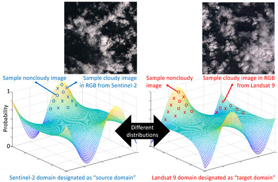
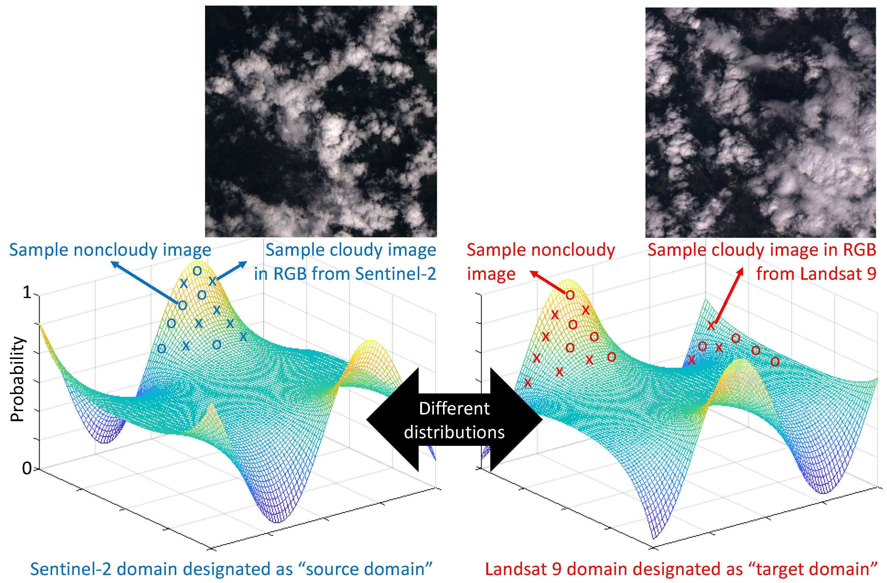
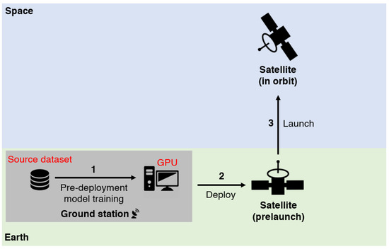
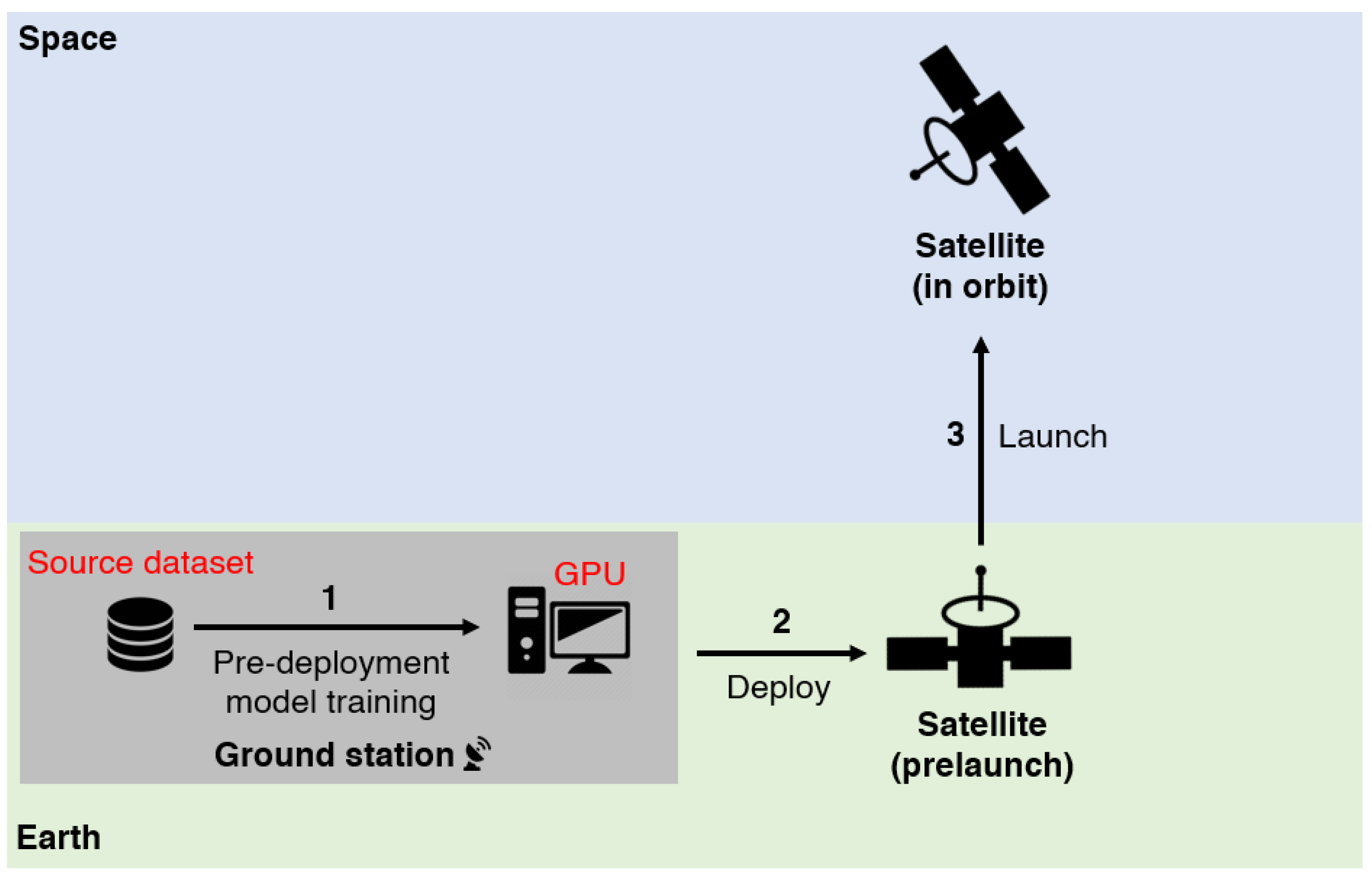
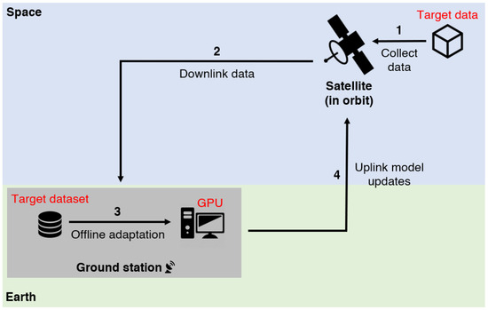
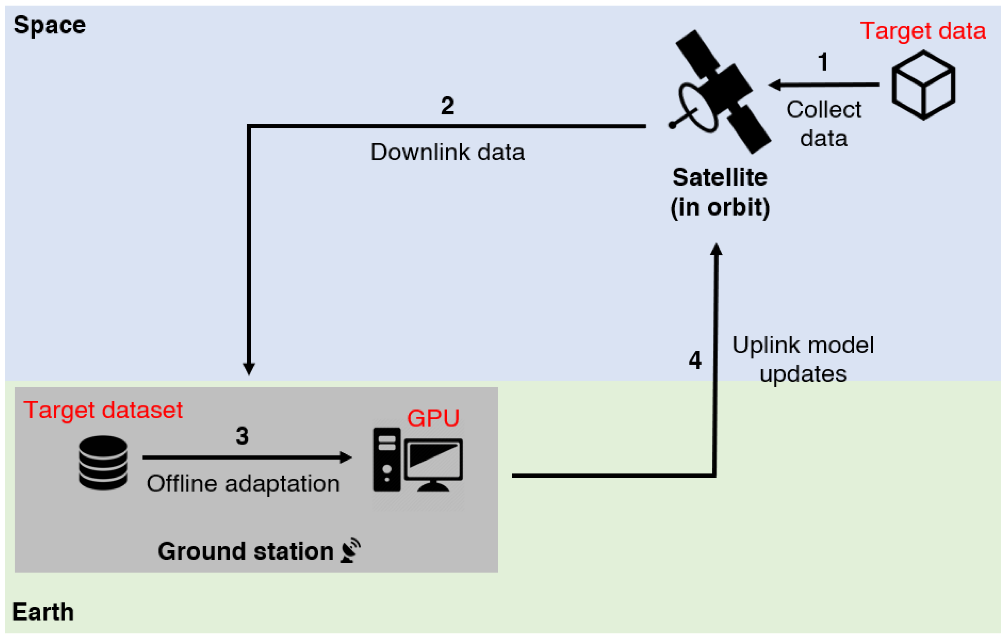
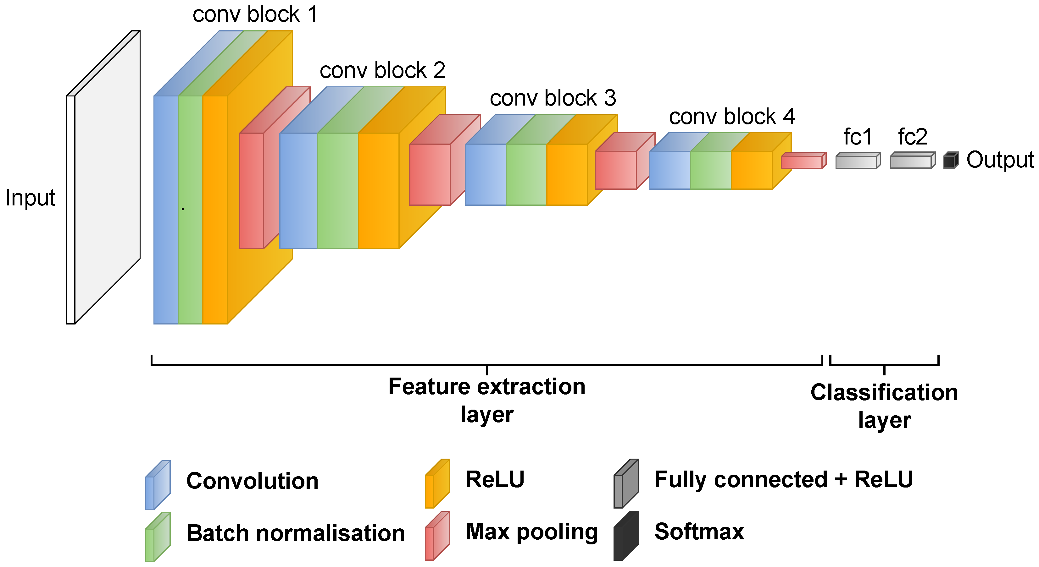
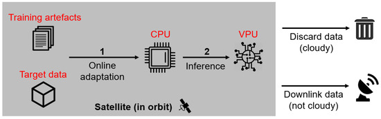
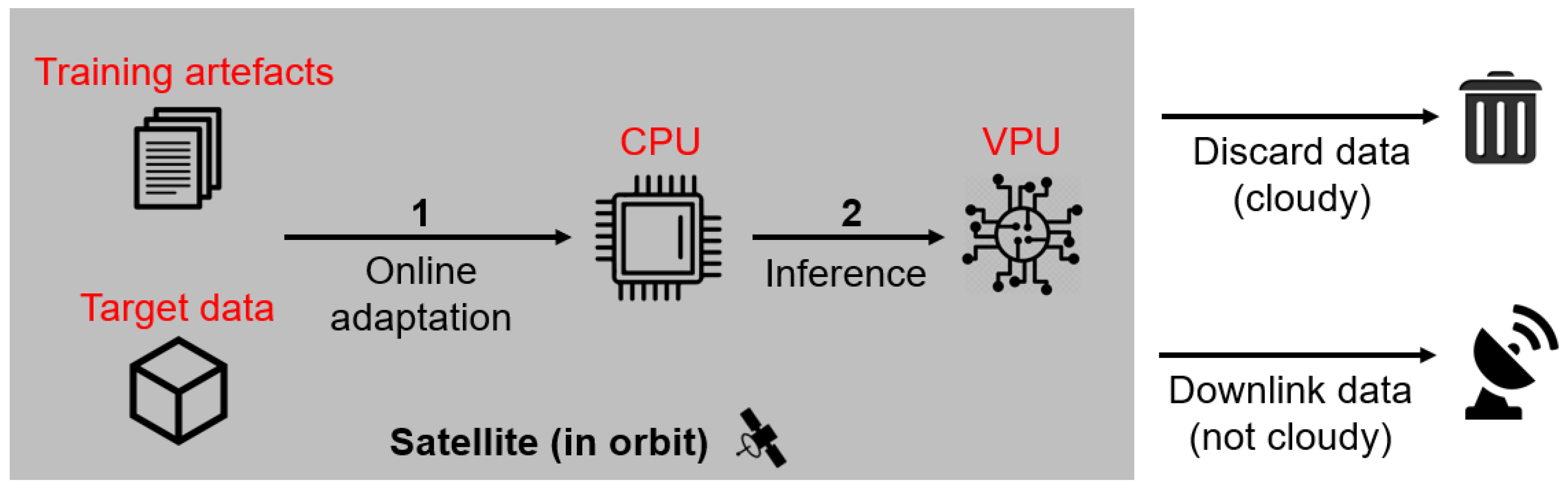
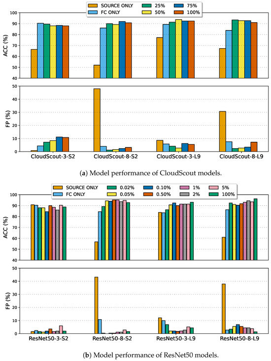
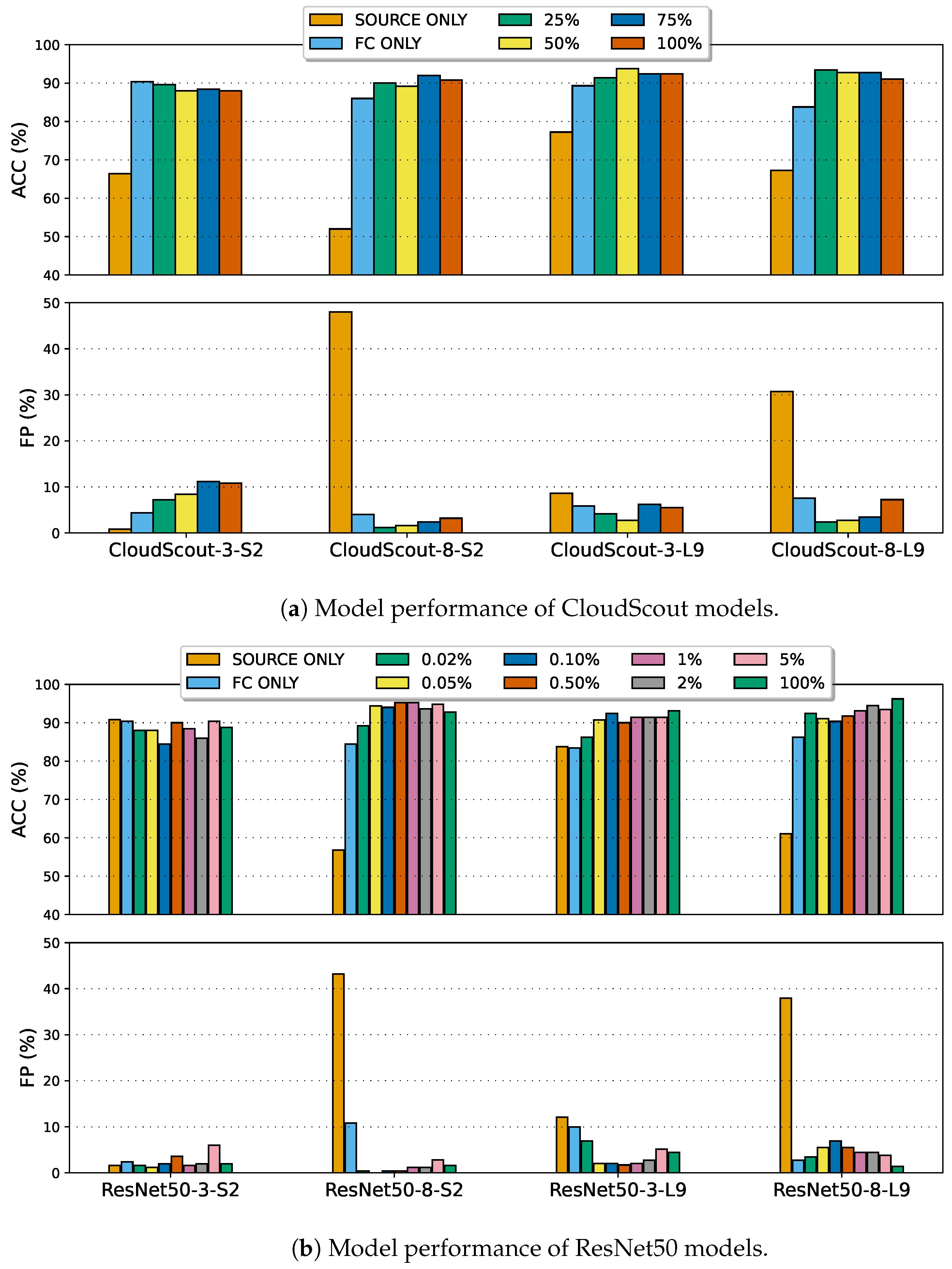
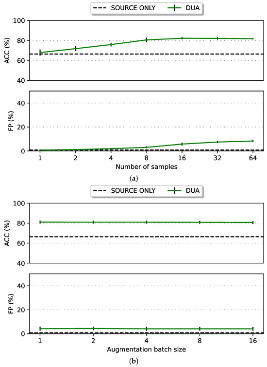
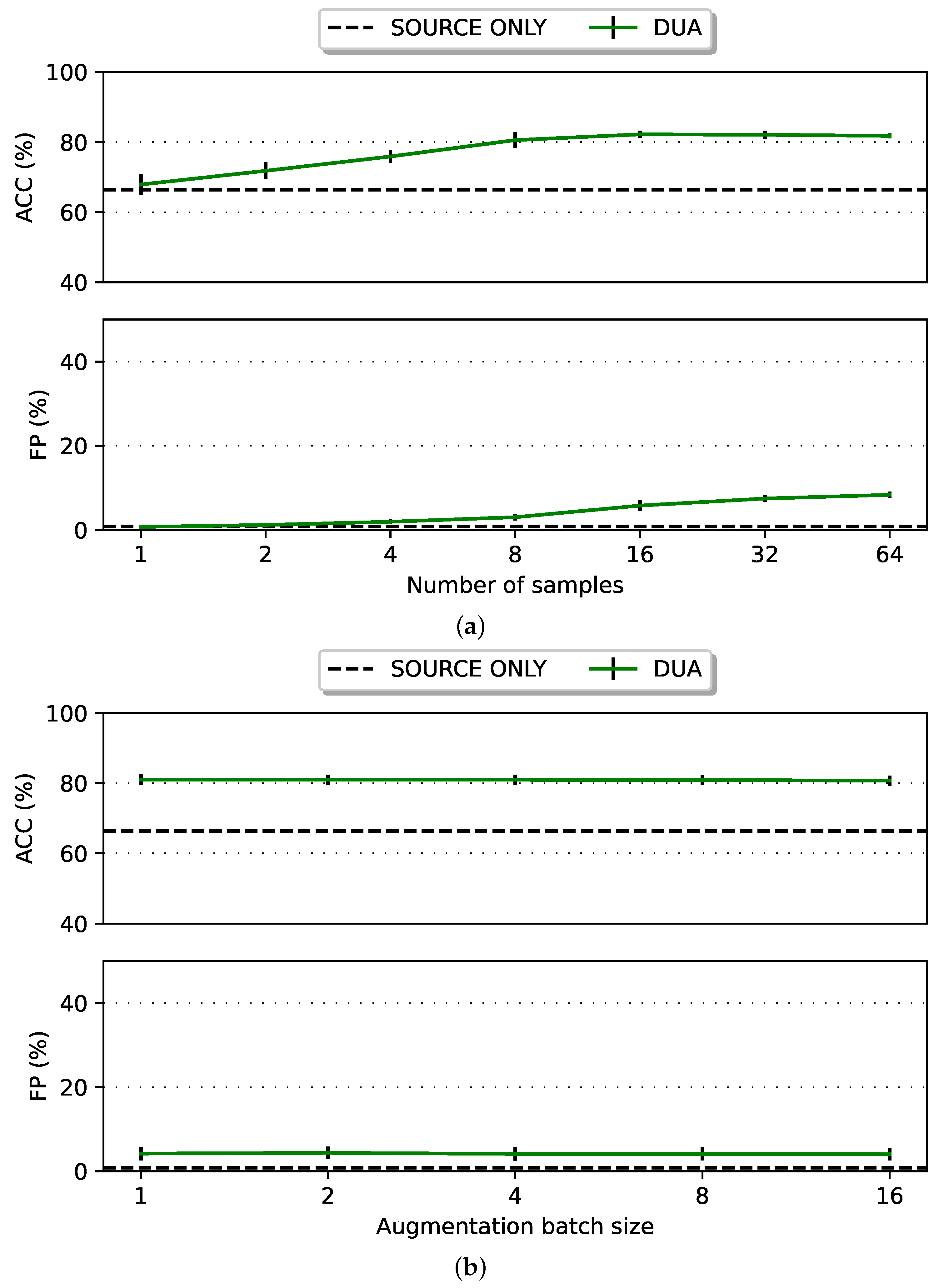
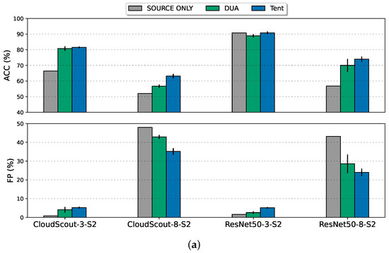
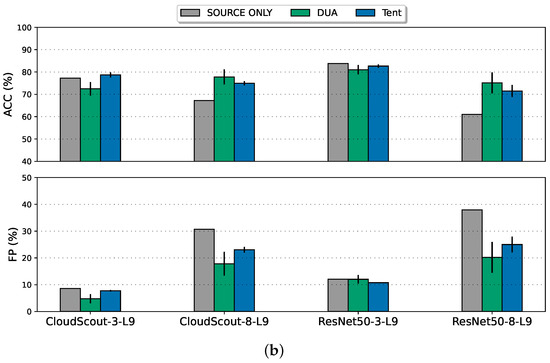
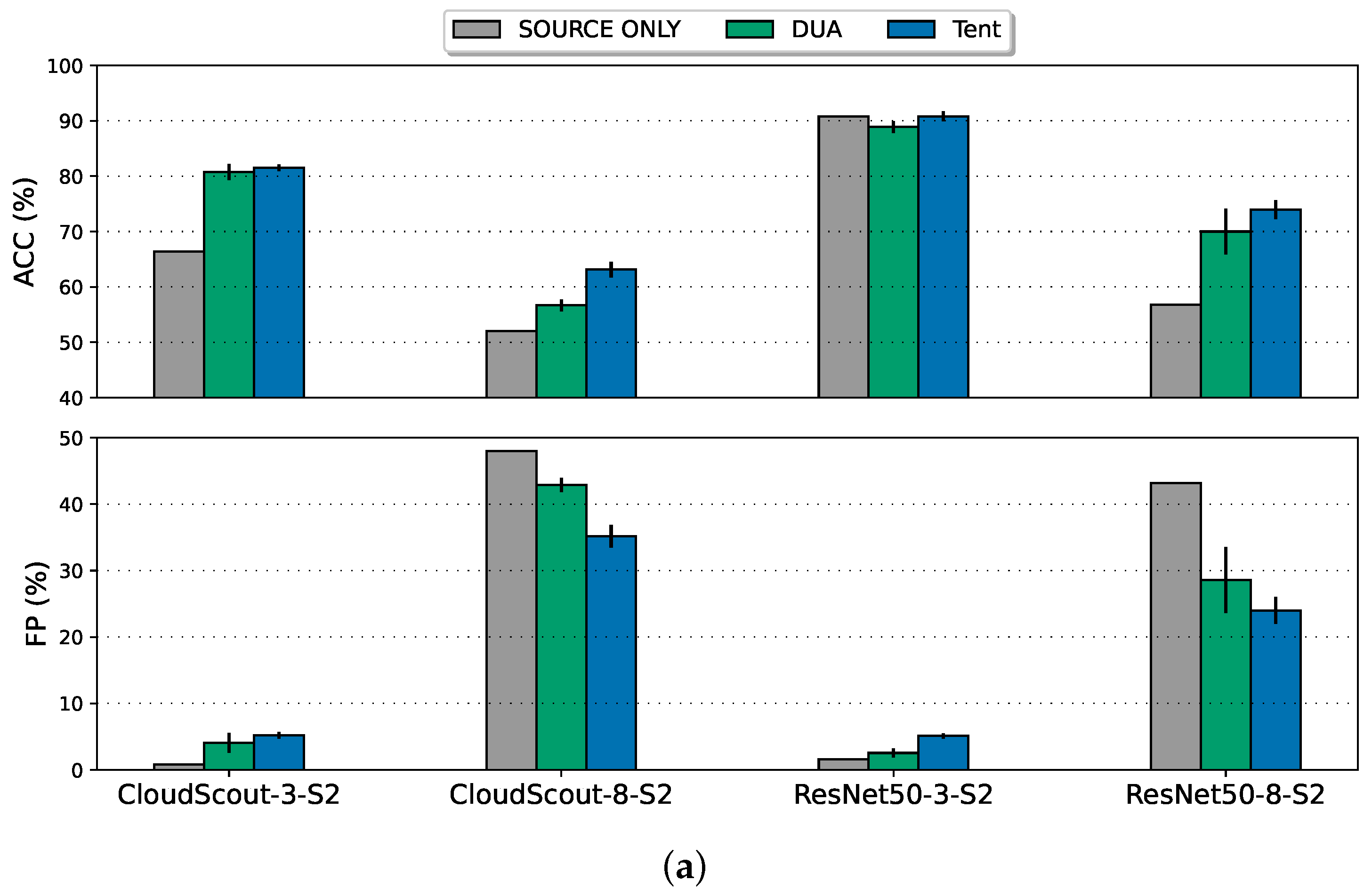
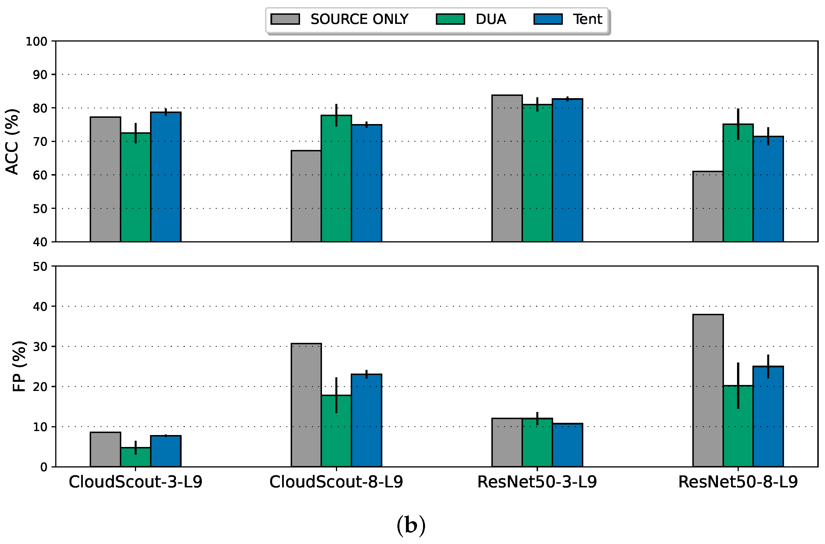
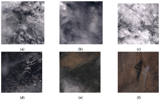
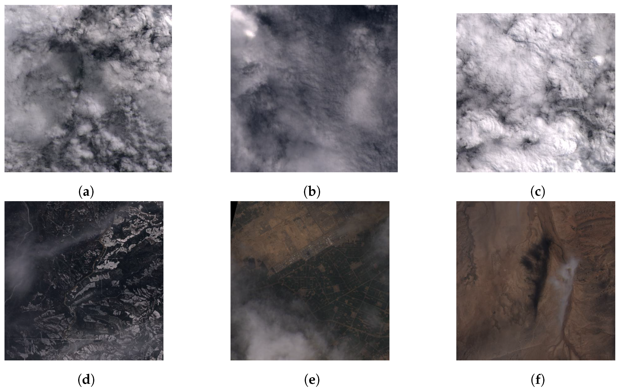

Disclaimer/Publisher’s Note: The statements, opinions and data contained in all publications are solely those of the individual author(s) and contributor(s) and not of MDPI and/or the editor(s). MDPI and/or the editor(s) disclaim responsibility for any injury to people or property resulting from any ideas, methods, instructions or products referred to in the content. |
© 2024 by the authors. Licensee MDPI, Basel, Switzerland. This article is an open access article distributed under the terms and conditions of the Creative Commons Attribution (CC BY) license (https://creativecommons.org/licenses/by/4.0/).