Efficient Lightweight Surface Reconstruction Method from Rock-Mass Point Clouds

Abstract

As for rock numerical calculation and stability analysis, it is essential to build a numerical model of rock mass with concise and accurate structure information through the three-dimensional surface reconstruction of rock-mass point clouds. However, the current research on lightweight surface reconstruction of non-artificial objects is very limited. In this paper, an efficient lightweight surface reconstruction method for rock-mass point clouds is proposed. Firstly, the input point cloud is segmented to obtain the plane primitives. In this process, the recognition of texture information and the complete over-segmentation of effective information play a vital role in the high-precision segmentation of rock surfaces. Secondly, the boundaries of all planes are reorganized according to the obvious connectivity in the segmentation results, so as to realize the assembly of the model, while solving all collision problems. Finally, an integer programming model is constructed to screen the best closure scheme of each plane, thus ensuring the best outcome of the reconstruction. In this study, seven groups of natural rock-mass point clouds are used to validate the proposed method. As suggested by the experimental results, this algorithm is effective in compressing the point cloud data of rock mass, to generate a watertight numerical model that can be directly used for simulation calculation. In addition, this method has strong robustness to noise and can effectively deal with highly corrupted rock-mass point cloud data.

1. Introduction

Whether an artificial target or a natural target, it is of great significance to obtain its structure information. The acquisition of structural information can be realized by surface reconstruction of point cloud data of the target. However, point cloud data of some nature targets may carry a certain amount of unavoidable texture information and noise. For this reason, it is usually inadvisable to retain all the details of the original point cloud in the reconstruction results for some large-scale reconstruction tasks [1,2,3], because the highly complex mesh structure can affect the efficiency and accuracy of subsequent operations. In recent years, lightweight surface reconstruction technology has attracted extensive attention in the field of computer vision and information processing.

Lightweight surface reconstruction refers to the technology of constructing a simple mesh model to represent the target surface structure. Different from dense mesh reconstruction technology, lightweight surface reconstruction only focuses on the main structure information of the target. Therefore, it can better filter the texture information and simplify the complexity of the model. At present, the available lightweight surface reconstruction methods are mainly to process artificial targets (buildings and man-made models) [1,2,4,5,6,7,8], for the purpose of extracting the contour information of the object and achieving data compression. In respect of rock-mass engineering, the significance of constructing a rock mass model with simple and accurate surface information goes further than that. Such methods as block theory [9] and discontinuous deformation analysis [10] have been demonstrated as effective in carrying out analysis of the rock masses for their stability [11]. In this process, it is essential to adopt a concise numerical model with accurate surface information (without texture information) as input. In particular, to carry out the subsequent block cutting process smoothly, the constructed rock mass model shall be made as simple as possible, without any highly complex grid structure (extremely small angle). Therefore, the lightweight surface reconstruction of rock mass point clouds is not only a problem needing to be solved for computer vision, but plays a significant role in the related numerical simulation calculations in the geotechnical field. Up to now, however, there is still limited research on the lightweight surface reconstruction of natural targets.

Laser scanning technology has the characteristics of high precision and non-contact, so it is widely used in the acquisition of natural rock mass data. However, different from the reconstruction of buildings, there are some special cases that should be considered and solved when processing point cloud data of natural targets, which can be summarized in the following three respects. First of all, due to geographical limits, natural conditions, and other influencing factors, it is practically difficult to ensure the quality of data on the rock-mass point cloud as collected from nature. In addition, the surface structure in some regions is extremely irregular, which can cause a further loss of surface information during surface segmentation. Therefore, how to deal with highly corrupted data is the key problem to be solved in rock mass surface reconstruction. Secondly, due to the complexity of surface structure, some errors need to be accommodated during the process of rock-mass surface segmentation, which may result in a deviation between the plane parameters and the real surface information to some extent. Due to the varying degrees of deviation between planes, there are various collision problems that may arise from the reconstruction. Finally, the boundaries of rock surface structural planes are usually irregular, which means that the shape information of boundaries is unfit for direct use in the reconstruction of the model. On the contrary, careful consideration shall be given to the simplification of these irregular shapes to ensure the simplicity of the model.

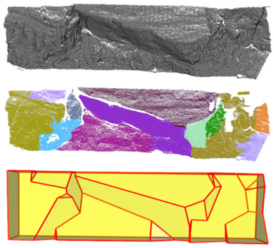
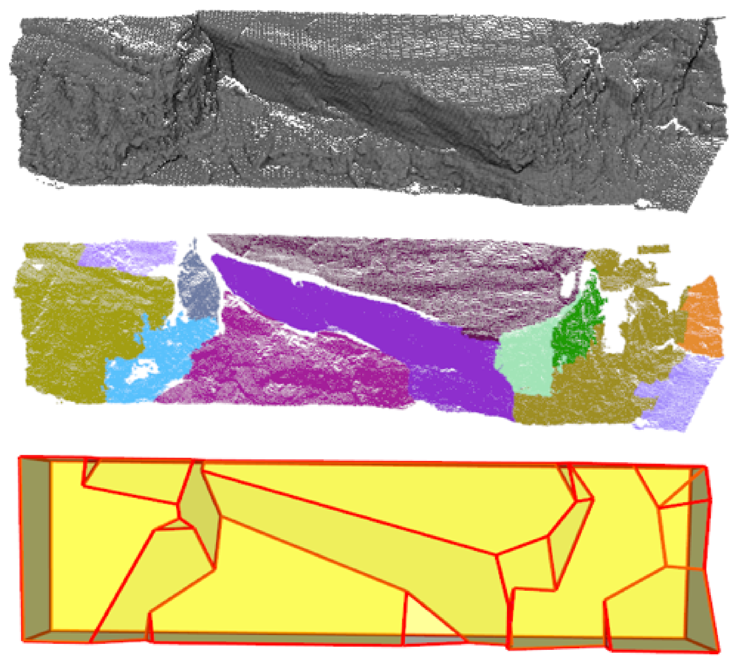
In order to address the above-mentioned problems, a lightweight surface reconstruction method is proposed in this paper from rock-mass point clouds. Figure 1 shows an example of reconstruction. For each input point cloud, a surface segmentation method based on supervoxel is adopted to determine initial planar primitives. In order to make the generated model watertight, the segmentation result is added with an outer bounding box. In the process of generating the basic model, the line segments and their initial lengths in the model are obtained based on the connectivity of the patches and their true edge information. The corner points determined to exist in the model are calculated to complete the closure of local areas. Then, in order to determine the boundaries of missing areas, boundary prediction is performed. The coverage rate and the matching rate are taken as indicators to measure the results of boundary prediction in each plane. The final result of reconstruction is obtained through triangle segmentation of holes.

Figure 1. Algorithm flowchart. (a) Input point cloud. (b) Surface over-segmentation result. (c) Segmentation result. (d) Basic model. (e) Plane closure. (f) Reconstruction result.

The contributions of this paper are detailed as follows:

• A framework of lightweight surface reconstruction was proposed, which is effective in processing the natural rock-mass point cloud to construct a numerical model with accurate and concise surface information;
• A solution to rock mass surface segmentation based on supervoxel was proposed, which can realize the effective segmentation of complex rock surface;
• The hole search problem in a 3D point cloud was converted into the boundary prediction of 2D planes. An integer programming model was constructed to perform boundary prediction, so as to ensure the water-tightness of the model and the effectiveness of reconstruction.

This paper is structured as follows. The related work is introduced in Section 2. In Section 3, the proposed method is detailed. Then, the experimental results are presented and discussed in Section 4. Section 5 concludes the study, with a summary made and the future direction of research indicated.

2. Related Work

Over the past few decades, there has been plenty of research conducted on the surface reconstruction of point cloud for obtaining a dense mesh model of the target [12,13,14,15]. However, the model constructed using the above algorithm is often highly complex in structure and carries no clear structural plane information of the target. In recent years, there has been widespread attention brought to the extraction of geometric primitives from the point cloud and assembling them for the building of a simple polygonal mesh model. In this section, our focus is placed mainly on primitive extraction and primitive-based surface reconstruction.

Primitive extraction. In this part, we aim to achieve the effective segmentation of the target surface for extracting high-quality primitives. Currently, RANSAC [16] has been demonstrated as effective in segmenting the surface of buildings and artificial models [4]. In practice, the performance of RANSAC is determined by the probability that the optimal solution is obtained by a single sampling. It is supposed that there are N points in the whole set of points and the maximum plane (the best plane) is comprised of n points. Let P indicate the probability that one sample can be used to obtain the best plane, as shown in Equation (1).

$$P={\left(\frac{n}{N}\right)}^3.$$

(1)

That is to say, RANSAC is high efficient in dealing with simple structures. However, the segmentation of rock mass surface is obviously a more challenging task. Since the rock surface is rough and unpredictable, the complex surface structure of rock mass and a large amount of noise information will lead to a significant deterioration in the performance of RANSAC.

In order to improve the outcome of rock mass segmentation, there have been some novel methods of rock mass surface segmentation proposed. For example, Riquelme et al. [17] conducted principal component analysis to determine the coplanarity of adjacent points, based on which high-precision segmentation was achieved by Hough Transform (DSE). Leng et al. [18] proposed a multi-scale rock surface detection method based on HT and Region Growing(HT-RG), which is effective in dealing with the surface structures of different scales. Due to the high computational cost of HT, however, it is difficult to achieve high-efficiency segmentation using the above two methods. At present, the use of voxel segmentation to achieve the partial structured of the point cloud is an effective solution to improve the performance of the algorithm. For instance, Hu et al. [19] put forward an efficient method of detection, where RANSAC was applied to perform coplanarity detection locally. The final result was obtained through regional growth. Based on the detection of local coplanarity, Liu et al. [20] used HT for calculating the main direction to obtain the seed patch, thus improving the accuracy of regional growth(MOE). However, the coplanarity detection based on voxels is ineffective in constraining the effective information with a high degree of dispersion. Consequently, it is difficult to achieve high-precision detection using these methods.

In the reconstruction process, careful consideration shall be given to both the efficiency and precision of segmentation. Thus, our focus is placed on filtering the noise inside the patch and ensuring that the effective information in the point cloud is completely structured before the global calculation is performed.

Primitive-based surface reconstruction. The surface structure of the rock mass is distinctively irregular and unpredictable. For this reason, this article gives consideration neither to the potential relationship between primitives (such as parallel and orthogonal), nor to the repetitive structure or composite structure in the point cloud [5,21,22,23,24,25]. The methods used to assemble planar shapes into a simple mesh can be divided into two categories, which are the connectivity method and the slicing method.

Connectivity methods can be adopted to achieve model assembly according to the exact shape of patches and the connectivity relationship between patches. Therefore, this method is demanding on the shape of planes. Processing and assembling basic primitives are the two main steps in applying the connectivity method. Schindler et al. [26] proposed a new method of surface model reconstruction for the artificial environment, with a complete 3D segmentation framework provided. Under this framework, the relationship between planes was parameterized and classified, while the reconstruction goal was not limited to the orthogonal relationship. Arikan et al. [27] obtained effective vertices by simplifying the plane. With the effective vertices in the region paired under the restriction of the constraint set, the adjacent patches can be closed. For the missing areas in the data, manual intervention was performed to carry out the repair. Alliez et al. [28] classified the points, and then preserved the region with special structure in the point cloud(such as the corner) under Delaunay triangulation. In the meantime, a minimum cut formula combining structure, geometry, and visibility was proposed to achieve high-quality reconstruction. Holzmann et al. [29] used dense triangular meshes to repair the missing parts for ensuring the water-tightness of the constructed model.

Though the existing connectivity methods are capable to achieve efficient building reconstruction, they can hardly deal with the rock mass in an effective way. Since most rock mass planes show no regularity in shape, it is difficult to assemble connected primitives by means of their shape information. In addition, it is also an open problem to obtain the simplified grid representation of information loss regions. In this study, our focus is placed on addressing the dependence of the connectivity method on shape information and ensuring the model is watertight.

Slicing methods ignore the shape information of the plane, since all the points and boundaries in the output mesh are obtained through the parameter calculation. Thus, these methods are made more robust to complex data. Chauve et al. [30] were the first to propose an algorithm intended to automatically achieve concise and idealized 3D representation from the unstructured point data of real scenes. When primitives are processed, the slicing method can be used to address the structure loss caused by occlusion. Similarly, Verdie et al. [31] performed plane cutting using line segments obtained by point cloud fitting, which can simplify the contour of the model and solve the simple problem of information loss. After the plane contained in the scene was identified, Mura et al. [32] obtained the 3D complex of the target by means of plane expansion, based on which the volume reconstruction of the room was realized. Furthermore, a more efficient and robust method of point cloud lightweight reconstruction was proposed by Nan et al. [4] According to this method, all planes would be extended freely in the bounding box to obtain several slices. Then, the output model is constructed by screening all possible models. Coverage rate, matching rate and model complexity are used to assess the quality of the model. However, the performance of this method is constrained by its high computation cost when complex structures are dealt with. In addition, the constructed model might be made erroneous due to the high corruption of inputted data. On this basis, Bauchet et al. [33] proposed a dynamic reconstruction method. Rather than decomposing the space completely, it adopts gradual extension. The extension would be terminated after a collision. Though the above methods solve the high computing cost incurred by the algorithm effectively, the reconstruction error caused by the high corruption of the data persists.

During the process of rock mass surface reconstruction, it is common and inevitable to suffer data damage due to various factors. At the same time, the cumulative error may lead to the collision between planes. In the process of rock mass surface reconstruction, the above problems need to be carefully considered and solved.

3. Methodology

The method proposed in this study involves three main steps. Firstly, plane primitives are extracted through the surface segmentation of rock point clouds. Then, basic models are constructed using the edge information of the plane and the connection relationship between planes. Finally, the missing boundaries in the model are predicted to conduct the search and reconstruction of information-missing areas.

3.1. Surface Segmentation

Coplanarity detection. At the start of the algorithm, the coplanarity detection method based on voxel segmentation is adopted, which is effective in distinguishing obvious planes and discrete information. RANSAC is relied on to carry out a search for the best plane in each local space. It is worth noting that, in each local space, coplanarity detection can be performed repeatedly if there are sufficient remaining points. The first obtained patch is taken as a growth unit, while the rest facets are merged into the adjacent similar growth units.

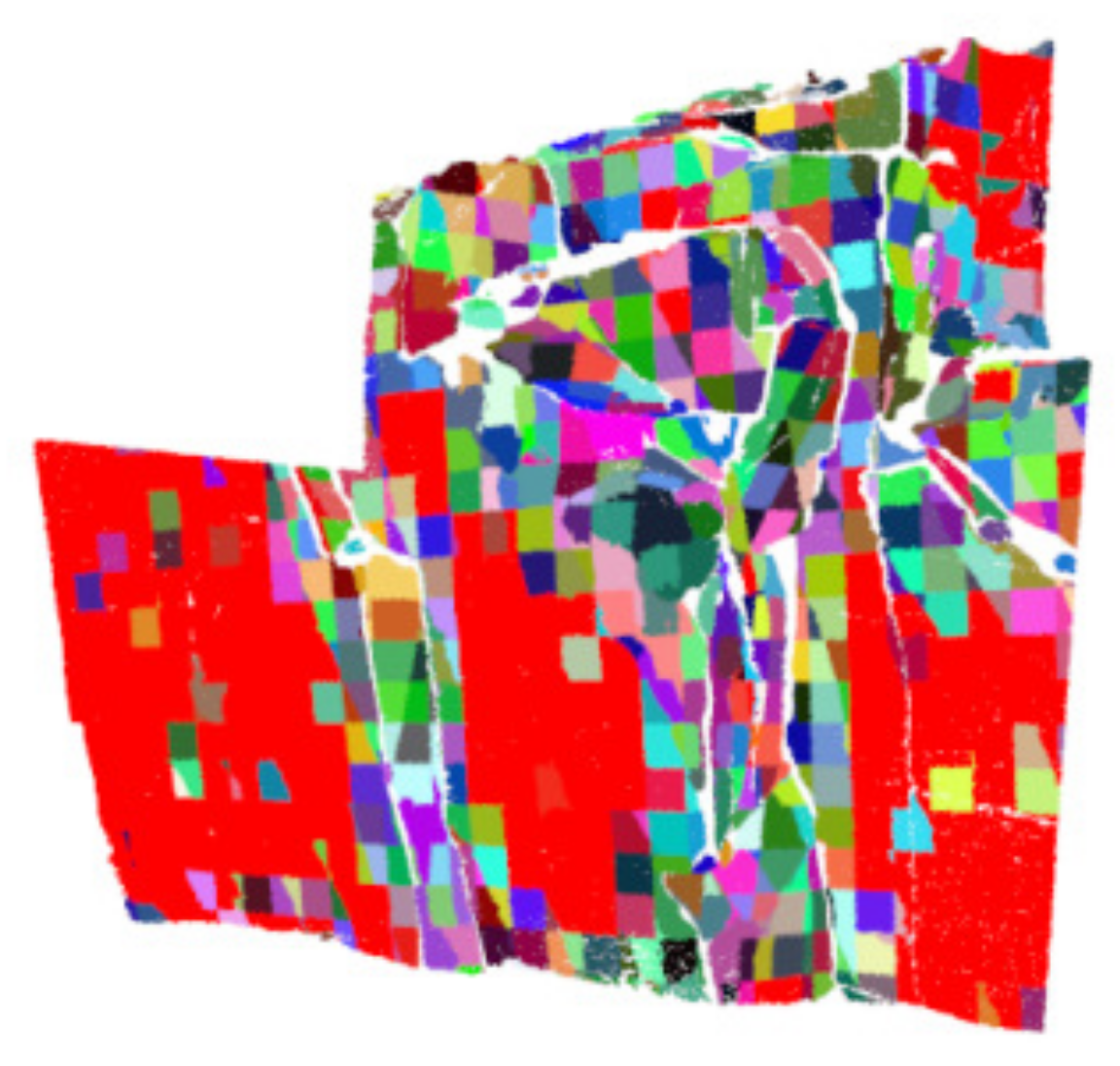
Texture information identification. In this paper, the identification of internal texture information is achieved by determining the position of discrete information. To achieve this purpose, a virtual region growth is performed for each growth unit to determine whether the patch can form a potential plane with all adjacent patches. In the case of successful growth, the growth unit is treated as an internal patch. The discrete information around the patch will be regarded as texture information rather than structure information, and will be ignored in the subsequent calculation process. The red area shown in Figure 2 is made up of the recognized internal patches.

Figure 2. Supervoxel segmentation in the boundary. Supervoxel patches are colored.

Supervoxel segmentation. After the internal noise is filtered, the supervoxel is used to process the discrete information accurately. More specifically, with each growth unit as a seed, the surrounding discrete information is incorporated into the seed depending on the exact judgment conditions including distance and angle. Furthermore, in order to ensure the effectiveness of the above process, it is necessary to ensure that the parameters of the growth unit do not change significantly. In this case, an effective growth is required to meet some additional conditions, as shown in Equation (2).

$$P_n=\underset{P_o}{argmax}\left|\{p\left|p\in P_o,\angle (\overrightarrow{n}\left(P_o\right),\overrightarrow{n}\left(P\right))\right.<\theta \}\right|,$$

(2)

where $P_n$ represents the final growth result, P denotes the initial patch, and $P_o$ refers to the result after a growth. That is to say, the growth result with the largest number of points is retained when the angle change falls below the threshold. The above-mentioned process can be achieved through iterative growth and the updating to growth parameters.

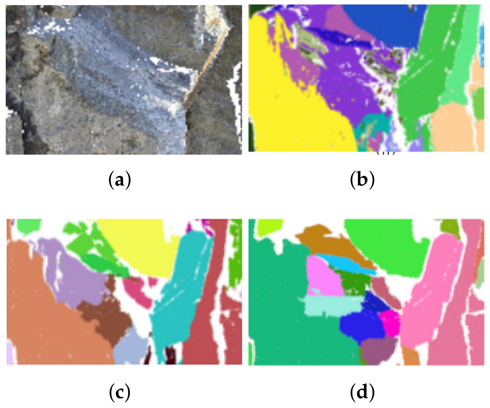
The essence of supervoxel segmentation is to achieve complete over-segmentation of surface structure and ensure complete structuring of effective structural information. Figure 3 shows the significance of structuring point clouds for dealing with complex surface structures. As more information gets integrated into the structured point cloud, the performance of the algorithm shows a significant improvement. Due to the achievement made in the complete over segmentation, there is more detailed information that can be retained.

Figure 3. Segmentation results under different structural degrees. (a) A surface area without clear boundaries. (b) Unstructured. (c) Semi-structured. (d) Completely structured.

Region Growing. After supervoxel segmentation, the surface segmentation problem is converted into a patch combination problem. The final result of segmentation is obtained by combining super voxel patches. Notably, the internal patches can be taken as seeds preferentially during growth, which lays a solid foundation of growth for the whole process. The segmentation process and reconstruction process conducted in our method are closely related to each other. As part of the adaptive adjustment, the setting of growth parameters will be discussed later(as shown in Section 3.2).

3.2. Basic Model Generation

Boundary reconstruction. Given that the shape information of the primitive contributes little to the initial stage of rock mass reconstruction, the boundaries of a primitive should be reconstructed. More specifically, these two planes are potentially continuous if there are only two planes in the local space. In order not to miss all possible potential relationships, multi-scale voxel division is performed to carry out search repeatedly. Suppose U is the set of connection relations as obtained by plane P after the i-th search, then the final connection relation set $U_f$ of P can be calculated using Equation (3):

$$U_f=U_1\cup U_2\cup U_3...\cup U_i.$$

(3)

Suppose Q is an element of $U_f$, then the intersection line of P and Q can be calculated. By calculating the minimum distance between the plane and the intersection line l, it can be determined whether the intersection line exists (as shown in Equation (4)).

$$\left\{\begin{array}{c}\underset{p\in P}{min}d(p,l)<d_h\\ \underset{q\in Q}{min}d(q,l)<d_h,\end{array}\right.$$

(4)

where p and q represent points in the plane, and $d_h$ refers to the threshold. At the time of boundary reconstruction, only the intersection line that satisfies Equation (4) can be retained. Thus, some approximately parallel structures can be excluded.

Furthermore, the initial length of each intersection line is calculated according to the edge information of related planes. Let $P_l$ denote the part related to the straight line l in the edge information of the plane P, which can be expressed as Equation (5).

$$P_l=\left\{p\left|d(p,l)<d_h,p\in P\right.\right\}$$

(5)

Let $P_w$ denote the vertical projection of $P_l$ on l. Similarly, the relevant information $Q_l$ and $Q_w$ of patch Q can be obtained as well. Only when Equation (6) is satisfied, can the connectivity between a set of patches be considered reliable and obvious.

$$\left|P_w\cap Q_w\right|>L_h,$$

(6)

where $L_h$ indicates the threshold. In the final boundary set, only the intersection lines calculated by the clear connection relation are retained, with the effective range of the intersection lines treated as the coincident part of the projection.

During our process of reconstruction, the assembly of primitives is carried out in the first place. However, the boundary structure of each plane is made open at present, as shown in Figure 4b. This problem will be resolved gradually in the follow-up process.

Figure 4. Basic model generation. (a) The connectivity information of a plane and related edge information. (b) Boundary reconstruction. (c) Corner calculation. The black circle area in the figure is closed by adding triangular patches.

Corner calculation. The corner points in the model are obtained by calculating the common points of the three planes which conform to the connection relationship. Then, one endpoint of the intersection line is extended to the corner for completing the local closure. In particular, when the extended distance is made overly long by cumulative error, this local region is closed by adding a triangular patch. It is worth noting that the local space created by the selected three endpoints does not contain other structures is the premise of corner calculation.

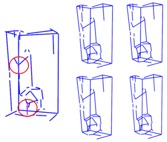
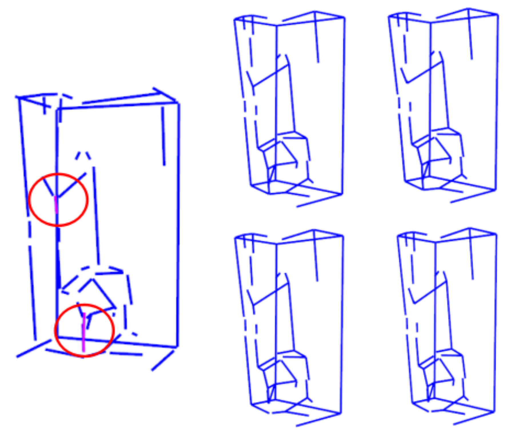
In case of an intersection or potential intersection in the boundary set, then the selection of endpoints will become problematic (as shown in Figure 5a). In this study, all possible results are retained, which means there are multiple candidate models preserved after corner calculation (as shown in Figure 6). During subsequent boundary prediction, different corner selections will lead to the difference of the shape to the final boundary (Figure 5c,d); this shape information will be used as the basis for screening the optimal reconstruction results. In practice, an inappropriate endpoint selection can lead to the failure of boundary prediction in many cases (Figure 5e).

Figure 5. Corner selection. The red point is the corner obtained by calculation. The green dotted line is the boundary obtained after subsequent boundary prediction. (a) An example of potential intersection. (b) A potential intersection in a set of boundaries. (c) Let D to perform corner calculation. (d) Let C to perform corner calculation. (e) A wrong boundary prediction result.

Figure 6. Some basic models generated due to the corner selection. Collision areas are shown in the red area on the left.

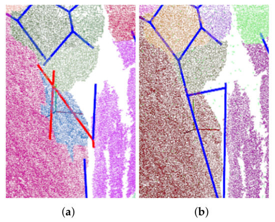
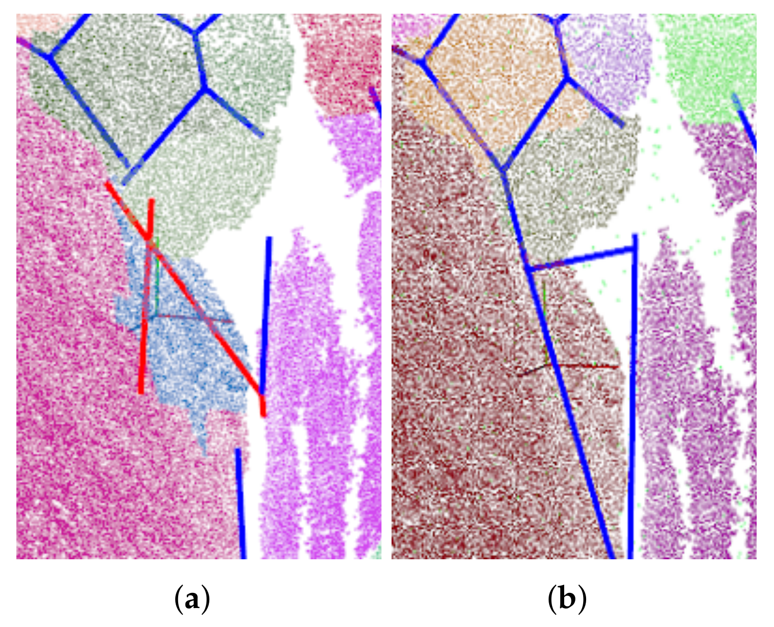
Adaptive adjustment (Collision detection). Due to the impact of cumulative error, there is a real possibility that collisions occur between planes. After boundary reorganization, the collision occurring between patches is indicated by the crossing of boundaries. During actual corner calculation, some collisions can be resolved, but those collisions failing to meet the conditions of corner calculation must be repaired through adaptive adjustment. Herein, it is proposed to divide the frequently-used parameter interval of supervoxel merged into the high-precision initial segmentation interval (used in region growing) and adaptive interval. The segmentation results obtained using the initial segmentation parameters are referenced to perform the first boundary reconstruction. In the area of collision, the similarity of the involved planes is calculated through Equation (7).

$$P_s=\sqrt{{\left(\frac{m_a}{M_c}\right)}^2+{\left(\frac{n_a}{N_c}\right)}^2},$$

(7)

where $m_a$ and $n_a$ represent the actual angle and distance deviation, while $M_c$ and $N_c$ refer to the thresholds. Within the range of adaptive threshold, a more similar set of planes should be merged (as shown in Figure 7). The supervoxel segmentation and division of parameter interval are purposed to eliminate the risk of under-segmentation from the reconstruction process. Therefore, all collision problems encountered in the reconstruction process can be attributed to over-segmentation.

Figure 7. Adaptive adjustment. (a) An example of the collision area. (b) The reconstruction result without collision.

In essence, adaptive adjustment is purposed to adjust the segmentation results according to the current state of reconstruction. After the adjustment, the composition of the plane set and the connection relationship could have changed, which makes it necessary to recalculate the boundary information of each plane. The effective basic model free from intersection problems can be constructed by one-off iteration or multiple iterations.

It should be noted that not all collision problems can be solved by adaptive adjustment, because the rock surface is completely irregular. Thus, when multiple groups of collision problems exist in a local region, manual intervention is still necessary.

3.3. Model Closure

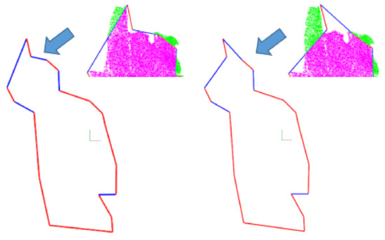
Boundary prediction. In this section, the missing boundary is predicted according to the exact shape of the patch and the available model information. For each plane, all of the non-corner endpoints in the boundary set are extracted and paired, with each pair of points connected by a line. Among all possible pairings, the pairing results which are completely connected but with no intersection are retained. Moreover, the final boundary set of P is determined according to the current state of the point cloud. In this method, there are two indicators used to assess the quality of a new group of boundary, including coverage rate and matching rate.

The coverage rate indicates the ability of the area formed by the new boundary to cover the original data. Let G represent a set of feasible new boundaries as obtained by boundary prediction and $P_n$ represent the set of points contained in G, then the coverage rate of $P_n$ can be calculated using Equation (8).

$$C=\frac{\left|\left\{p\left|p\in P_n,p\in P\right.\right\}\right|}{\left|\{p\in P\}\right|},$$

(8)

where p represents the point in the original point set P. In general, the effectiveness of reconstruction can be ensured by maintaining patch coverage.

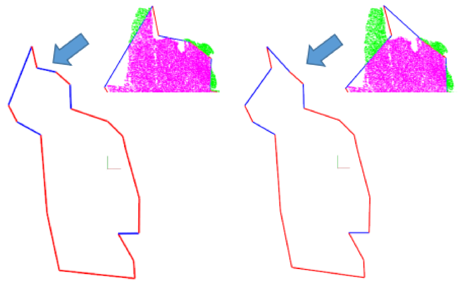
Since some boundary sets with high coverage may create some redundant space, it is worthwhile to consider introducing the matching rate to address this problem. In order for a fast search of the boundary distant from the original data, all parts of the boundary set which are tangent or intersect with the point cloud are considered as matching (as shown in Figure 8). Therefore, the matching rate can be calculated using Equation (9).

$$M=\frac{\{L_m\left|\underset{p\in P}{min}d(p,L_m)<L_h,L_m\in G\right.\}}{G},$$

(9)

where $L_m$ represents the matching part of G. In order to calculate $L_m$, it is necessary to determine the range of the line segment that matches the data by performing a fixed radius search of each point in the plane. To simplify the calculation process, the matching length of a line segment is obtained via equidistant sampling.

Figure 8. Two sets of feasible boundary sets. When the coverage is close, the boundary set that produces less redundant space will be selected. (Left): M =95.6%,C = 94.9%. (Right): M = 95.1%, C = 93.4%.

Based on the above information, the integer programming model intended to perform boundary prediction can be expressed as Equation (10).

$$\begin{array}{c}\underset{X}{min}{\lambda }_c·C+{\lambda }_m·M\hfill \\ s.t.\left\{\begin{array}{c}{\displaystyle \sum _{j\in P_b}}{x}_{ij}=1,\forall i\in P_a\hfill \\ d(x_{ij},g)>0,\forall x_{ij}=1,g\in G_l\hfill \\ \left|G_n\right|=\left|P\right|\hfill \\ x_{ij}\in \{0,1\},\forall i\in P_a,j\in P_b,\hfill \end{array}\right.\hfill \end{array}$$

(10)

where $P_a$ represents the set of non-corner points of a plane. With a point $x_i$ in $P_a$ selected, $P_b$ represents the set of points that are possible to match $x_i$ (excluding itself and the points connected with $x_i$ in the original boundary set). ${\displaystyle \sum _{j\in P_b}}{x}_{ij}$ is used to count the number of times that $x_i$ is used in each round of pairing. $G_l$ represents the segment in G that has no common vertex with segment $x_{ij}$. $G_n$ refers to the set of connected points searched with any point as the starting point. The hard constraint in the formula is purposed to ensure that the final boundary set is not in an intersection and closed. Due to the limited number of non-corner points, the model can be solved quickly without any solver.

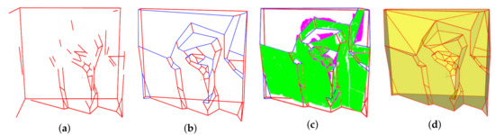
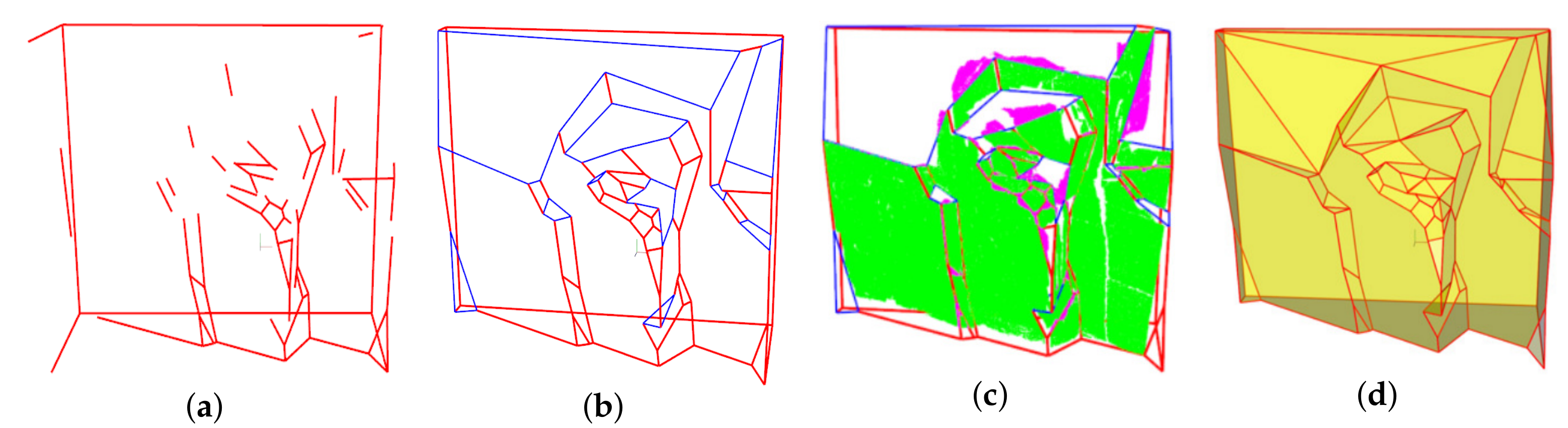
After optimization, the best set of boundaries can be obtained for each patch. When the boundary prediction is completed for all planes, the holes in the point cloud can be identified (as shown in Figure 9b). It is worth noting that in case of multiple candidate models, the global coverage and matching rate of each model shall be calculated to screen out the best outcome of the reconstruction.

Figure 9. Results of boundary prediction. The blue line segment represents the boundary obtained by prediction.(a) A basic model. (b) The best prediction result. (c) Effectiveness test. Covered points (green): 255,157. Remaining points (purple): 21,051. (d) The reconstruction result.

Model recovery and triangulation. After boundary prediction, there are some points in the point cloud that can not be covered by the model (as shown in Figure 9c). Among them, local information loss is made inevitable if it results from boundary reconstruction (cut by the red line). On the contrary, the information loss caused by boundary prediction can be repaired by means of model recovery. The process of repair is simple, just simplify the outer boundary of the uncovered point set and assemble it on the model. It is obviously easier to introduce explicit structure into the model than to deal with redundant faces, which is the reason why the boundary is allowed to appear inside the plane when the matching rate is calculated. Finally, the hole is triangulated to ensure that the final model is watertight.

4. Results and Discussion

This method was implemented in C++, and the Point Cloud Library [34] was used to process the point cloud. In this section, there are multiple groups of natural point clouds used to validate the proposed algorithm. All experiments were carried out on i7-7700, 3.60 Ghz and 4.00 GB ram without any parallel operation.

4.1. Datasets

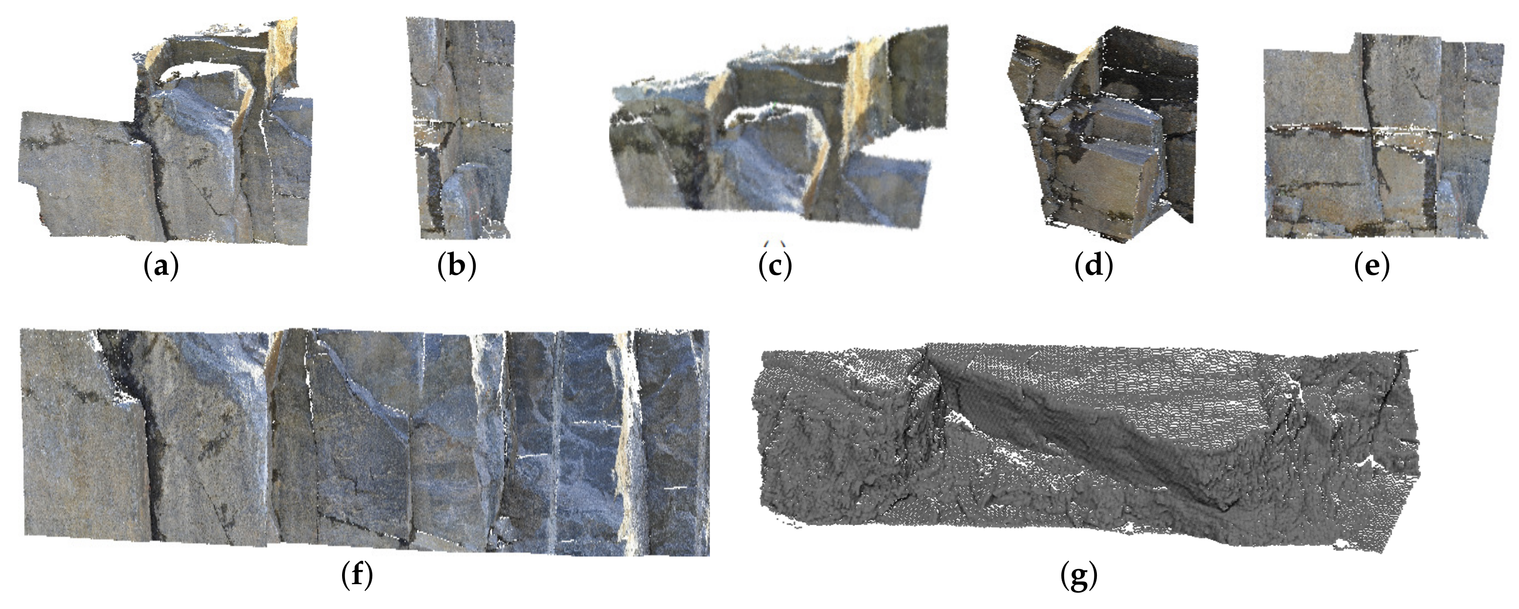
In this study, seven groups of natural rock mass point clouds are used as experimental data (as shown in Figure 10). The details of all data sets are shown in Table 1. The first six groups of data are from Rockbench repository [35], as obtained in Canada using Leica hds6000 scanner. The seventh group of data comes from the mountain dataset released by Wuhan University [36], which is collected by Scanstation C5 in the natural mountain. Specifically, Rock 1 has a complex surface structure, so it is used to test the effectiveness of the surface segmentation method. The reasons for the loss of surface information in Rock 2, Rock 3 and Rock 4 are different, so they are used to verify the effectiveness of the reconstruction method proposed in this paper in various situations. We performed comparative experiments using Rock 3 and Rock 5. In addition to the loss of a large amount of surface information, the former also has a more complex surface structure. The latter has good data quality and relatively simple surface structures. Rock 6 is used to demonstrate the ability of this method to process large-scale data and clarify the parameter adjustment required. Finally, Rock 7 is used to verify the effectiveness of the method on the mountain dataset.

Figure 10. Seven datasets. (a) Rock 1. (b) Rock 2. (c) Rock 3. (d) Rock 4. (e) Rock 5. (f) Rock 6. (g) Rock 7.

Table 1. Basic infomation of all datasets.

Data	Number of Points	Bounding Box
Rock1	$\mathrm{302,737}$	$27.13\ast 22.91\ast 10.38$
Rock2	$\mathrm{48,972}$	$10.21\ast 19.04\ast 6.19$
Rock3	$\mathrm{312,659}$	$28.8\ast 13.1\ast 11.9$
Rock4	$\mathrm{85,377}$	$9.5\ast 12.75\ast 4.66$
Rock5	$\mathrm{112,465}$	$23.81\ast 19.08\ast 6.19$
Rock6	$\mathrm{178,550}$	$48.5\ast 9.5\ast 6.84$
Rock7	$\mathrm{82,481}$	$11.6\ast 15.1\ast 5.1$

4.2. Parameter Settings

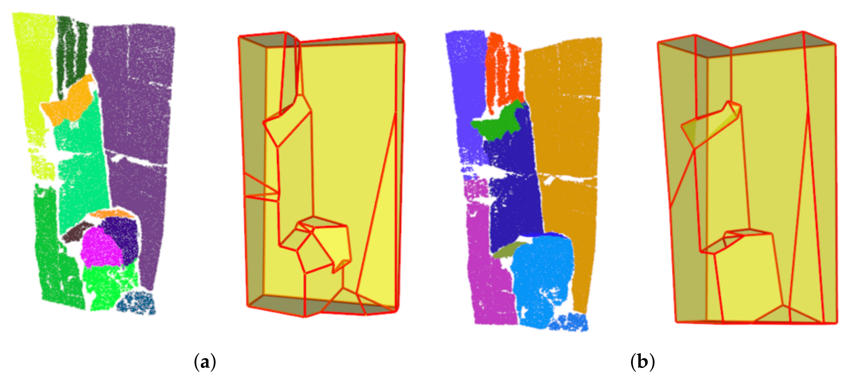
The main parameters involved in this method are the angle and distance thresholds used in the surface segmentation process. The valid range of parameters is from local (coplanarity detection) to neighborhood (supervoxel segmentation) to global (region growing and adaptive adjustment). Coplanarity detection is a critical step in surface segmentation, and high-precision parameters must always be used to ensure that surface structures can be over-segmented. The parameters used for supervoxel segmentation need to be slightly larger than those used for coplanarity detection, which helps to improve the effectiveness of surface segmentation (improve recall rate). The complexity of the final generated model is controlled by the parameters used in the process of region growing. The function of these parameters is to determine whether two or more supervoxel patches should be merged. The higher the accuracy of the parameters used for regional growth, the more complex the generated model will be and the more detailed information will be obtained (as shown in Figure 11). A simpler model can be obtained by using a larger threshold parameter. Although some structural information will be lost, the possibility of collision in the reconstruction process will be reduced. Therefore, it is necessary to use larger region growing parameters when processing large-scale data (Rock 6) or data with rough surfaces (Rock 7). The meaning and recommended value range of the main parameters involved in the method are shown in Table 2.

Figure 11. Segmentation and reconstruction results obtained using different region growing parameters. (a) $gro{w}_{dis}=0.18$, $gro{w}_{ang}={13}^{\circ }$. (b) $gro{w}_{dis}=0.23$, $gro{w}_{ang}={18}^{\circ }$.

Table 2. Information of parameters.

Stage	Parameters	Configuration Method	Meaning
Surface segmentation	$ra{n}_{dis}$	$0.08$–$0.12$ (m)	distance threshold of coplanarity detection
	$ra{n}_{ang}$	8–12°	angle threshold of coplanarity detection
	$supe{r}_{dis}$	$0.13$–$0.2$ (m)	distance threshold of supervoxel segmentation
	$supe{r}_{ang}$	13–${20}^{\circ }$	angle threshold of supervoxel segmentation
	$gro{w}_{dis}$	$0.13$–$0.23$ (m)	distance threshold of region growing
	$gro{w}_{ang}$	13–${23}^{\circ }$	angle threshold of region growing
Edge information calculation	$d_h$	$0.1$–$0.3$ (m)	radius length of boundary information search
	$M_c$	$0.18$–$0.25$ (m)	distance threshold of adaptive adjustment
	$N_c$	18–${25}^{\circ }$	distance threshold of adaptive adjustment
Model closure	$L_h$	$0.1$–$0.3$ (m)	distance threshold for matching degree calculation

4.3. Surface Segmentation Results

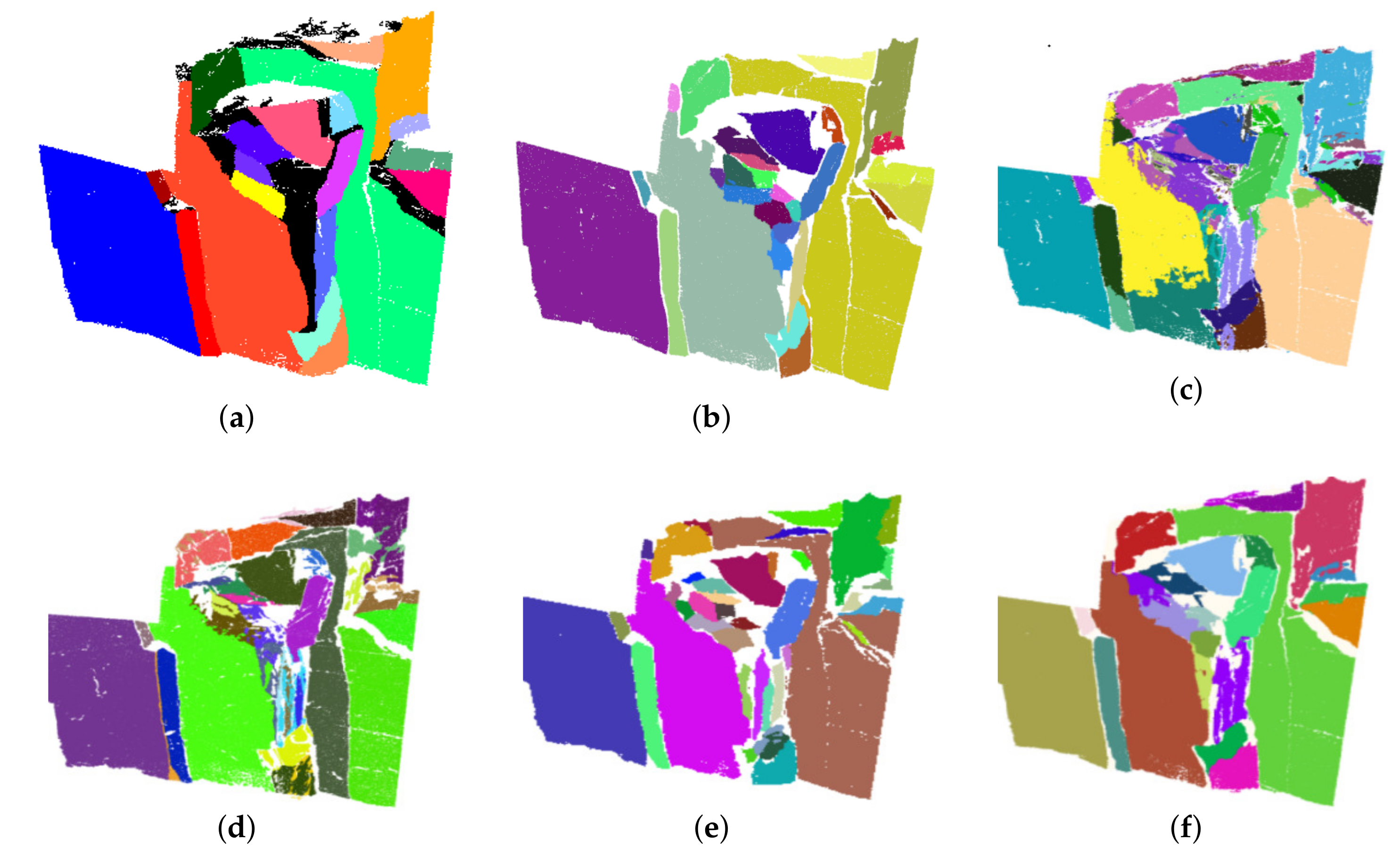
In this paper, we use Rock 1 to test and verify the surface segmentation method. The surface structure of Rock 1 is complex. In addition to large and clear structural planes, some small structural planes and transition planes are also concentrated in the data center. For quantitative comparison, we marked the surface structure of Rock 1. It is worth noting that the reference point cloud comprehensively considers the marking results of five researchers in the field of rock mass engineering and computer vision. In the final reference point cloud, some transition surface areas (black area) that were more controversial during the labeling process were not included. Therefore, the final reference point cloud is composed of structural surfaces with better planarity. In addition, we verified the structural surfaces in the reference point cloud using RANSAC to ensure the validity of the reference data. In the meantime, HT-RG [18], DSE [17], MOE [19] and PCL-RAN [20] (Ransac) were adopted as comparison methods.

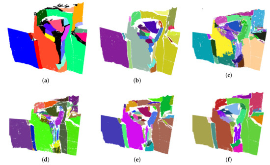
Figure 12 shows the segmentation results of Rock1 using different methods. Meanwhile, an evaluation system including accuracy, recall, and F1 [19] is employed to quantify the difference between the results and the reference point cloud. Table 3 lists the quantitative evaluation results produced using each method. The experimental results show that this method has obvious advantages in extracting clear structural planes. Since this method uses the over-segmentation strategy to segment the surface information, it has less under-segmentation and boundary problems while obtaining higher detection accuracy. By observing the segmentation results, it can be found that this method also realizes effective segmentation for some large transition surface areas (black areas), which can significantly improve the effectiveness of the method in processing more complex mountain data. Meanwhile, the efficiency of our algorithm (as shown in Table 4) is deemed acceptable. The reconstruction result of Rock 1 is shown in Figure 9.

Figure 12. Segmentation results. (a) Reference point clouds. (b) Ours. (c) PCL-RAN. (d) DSE. (e) HTRG. (f) MOE.

Table 3. Detection Results of Rock 1.

Method	Accuracy	Recall	F1
PCL-RAN	$79.5\%$	$83.3\%$	$81.4\%$
DSE	$85.4\%$	$79.5\%$	$83.5\%$
HTRG	$93.2\%$	$89.3\%$	$91.5\%$
MOE	$91.9\%$	$91.6\%$	$91.8\%$
Ours	$94.8\%$	$94.2\%$	$94.5\%$

Table 4. Execution time for different rocks (s).

Method Name	Rock1	Rock2	Rock3
PCL-RAN	$47.60$	$8.17$	$44.48$
DSE	$388.76$	$44.15$	$341.32$
HTRG	$198.41$	$29.17$	$164.78$
MOE	$2.13$	$1.12$	$2.56$
Ours	$9.47$	$3.27$	$8.15$

4.4. Robustness Test

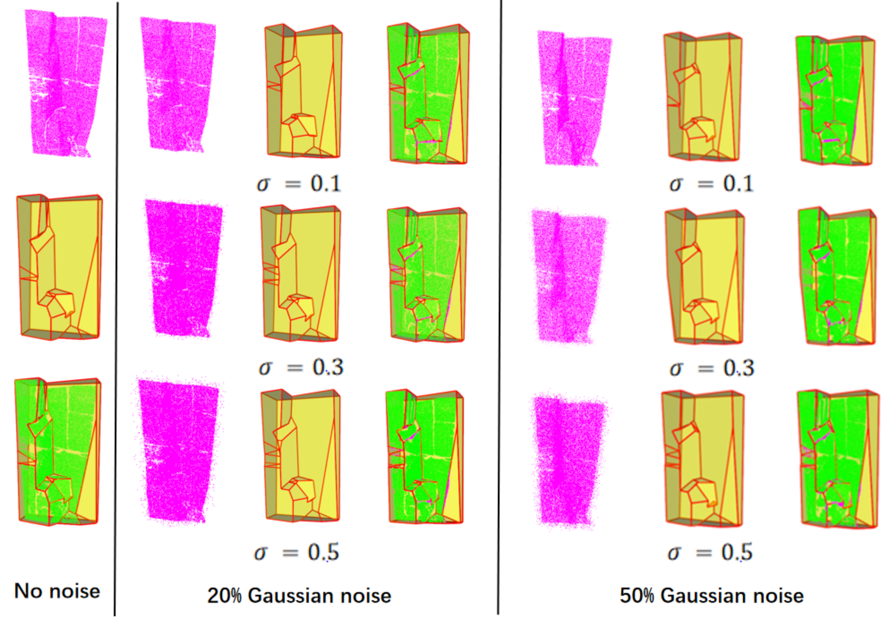
Firstly, we test the ability of this method to process noise data. For quantitative comparison, we take the reconstruction result and effective region of Rock 2 in the noise-free state as the reference value. Then, the effective area in the reconstruction results obtained under different noise conditions is taken as the real value. By calculating the RMSE of the reference value and the real value, the disturbance of noise to the reconstruction results is observed. RMSE can be calculated by Equation (11).

$$RMSE=\sqrt{\frac{1}{N}\sum _{i=1}^N{(p_i-{p_i}^{\prime })}^2}.$$

(11)

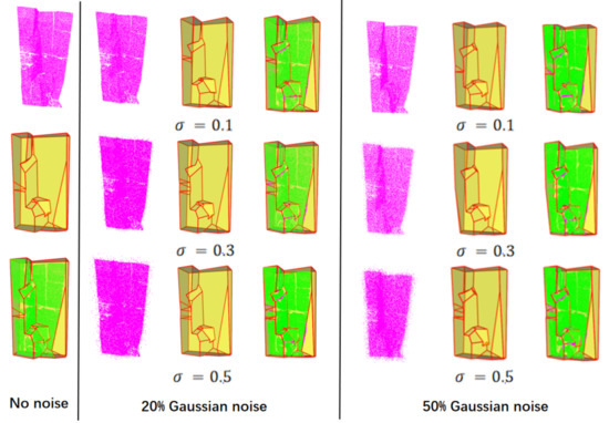
The reconstruction results under different noise conditions are shown in Figure 13. It can be seen from the figure that under different noise conditions, the main structure of the reconstruction results is basically the same and will not change significantly due to the noise data. The calculation results of RMSE under different noise conditions are shown in Table 5. With the increase of the number and level of noise, the impact of noise on the reconstruction process will be more obvious, but the error will be maintained in an acceptable range. The reason why the method proposed in this paper can effectively process noise data is that RANSAC is used as the local coplanarity detection method, and high-precision parameters are used for detection, which significantly improves the sensitivity and robustness of this method to noise.

Figure 13. Noise test. The three types of data in the figure represent the input data (in red), reconstruction result (in yellow) and effective region (in green).

Table 5. The information of noise test.

Noise	Parameters	RMSE
20% Gaussian noise	$\sigma =0.1$	$2.81$e$-02$
	$\sigma =0.3$	$2.86$e$-02$
	$\sigma =0.5$	$2.92$e$-02$
50% Gaussian noise	$\sigma =0.1$	$3.71$e$-02$
	$\sigma =0.3$	$4.24$e$-02$
	$\sigma =0.5$	$4.32$e$-02$

In addition, we further verify the effectiveness of this method in dealing with data with poor data quality. There are three main reasons for the poor quality of rock mass point cloud data. Firstly, there may be some concave structures on the rock mass surface, which makes some surfaces unable to be obtained due to occlusion. Secondly, the integrity of the data will be affected by the acquisition location. For example, when collecting data on the ground, it may be difficult to obtain surface information parallel to the ground. Finally, when part of the rock mass surface has no planarity, it is difficult to obtain effective structural information from this area, which will result in incomplete information included in the surface segmentation results. The above three cases will lead to the loss of surface information, and the loss of surface information may involve the loss of the whole plane, rather than the small holes in the plane.

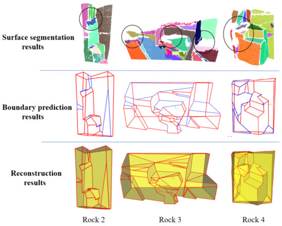
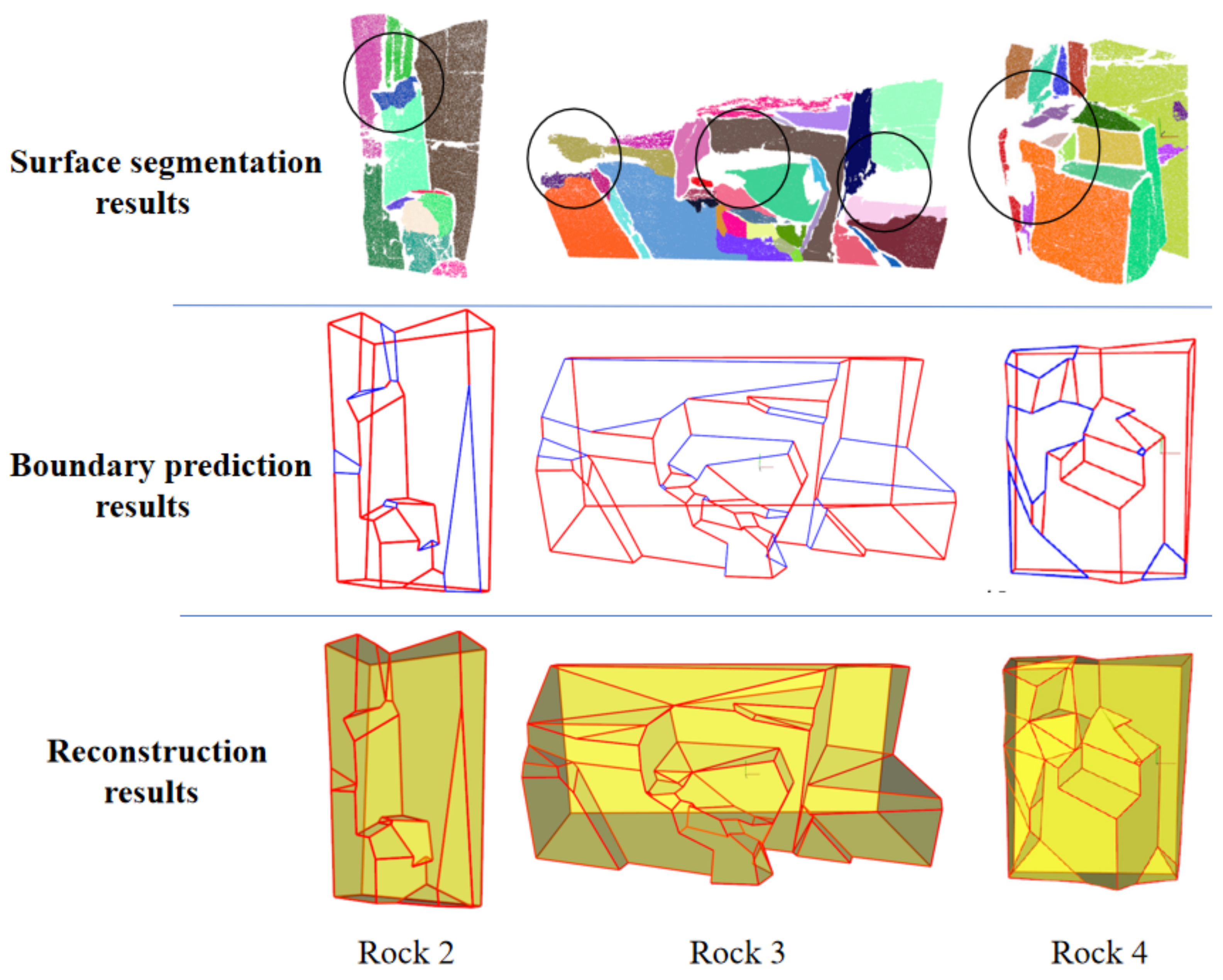
Therefore, we use Rock 2, Rock 3 and Rock 4 to represent the above three situations respectively. The boundary prediction results of information loss areas and final reconstruction results of each point cloud are shown in Figure 14. In this paper, on the basis of generating the basic model, the boundary prediction method based on an integer programming model is implemented, which can effectively deal with the loss of plane information caused by occlusion (Rock 2) and acquisition location (Rock 3). For the problem of missing information in the surface segmentation results caused by surface irregularities (Rock 4), this method can use a simple triangular mesh representation to repair holes, generate a closed model, and ensure the effectiveness of surface reconstruction in other areas.

Figure 14. Tests on datasets with poor data quality. Obvious information loss areas are marked by black circles.

4.5. Reconstruction Results

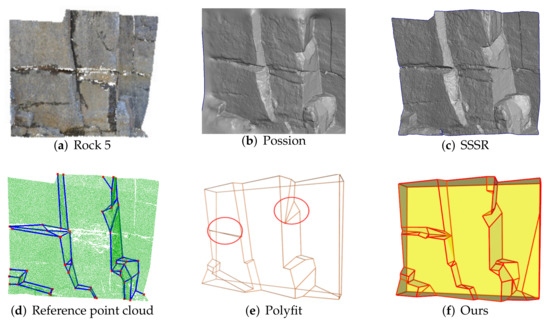
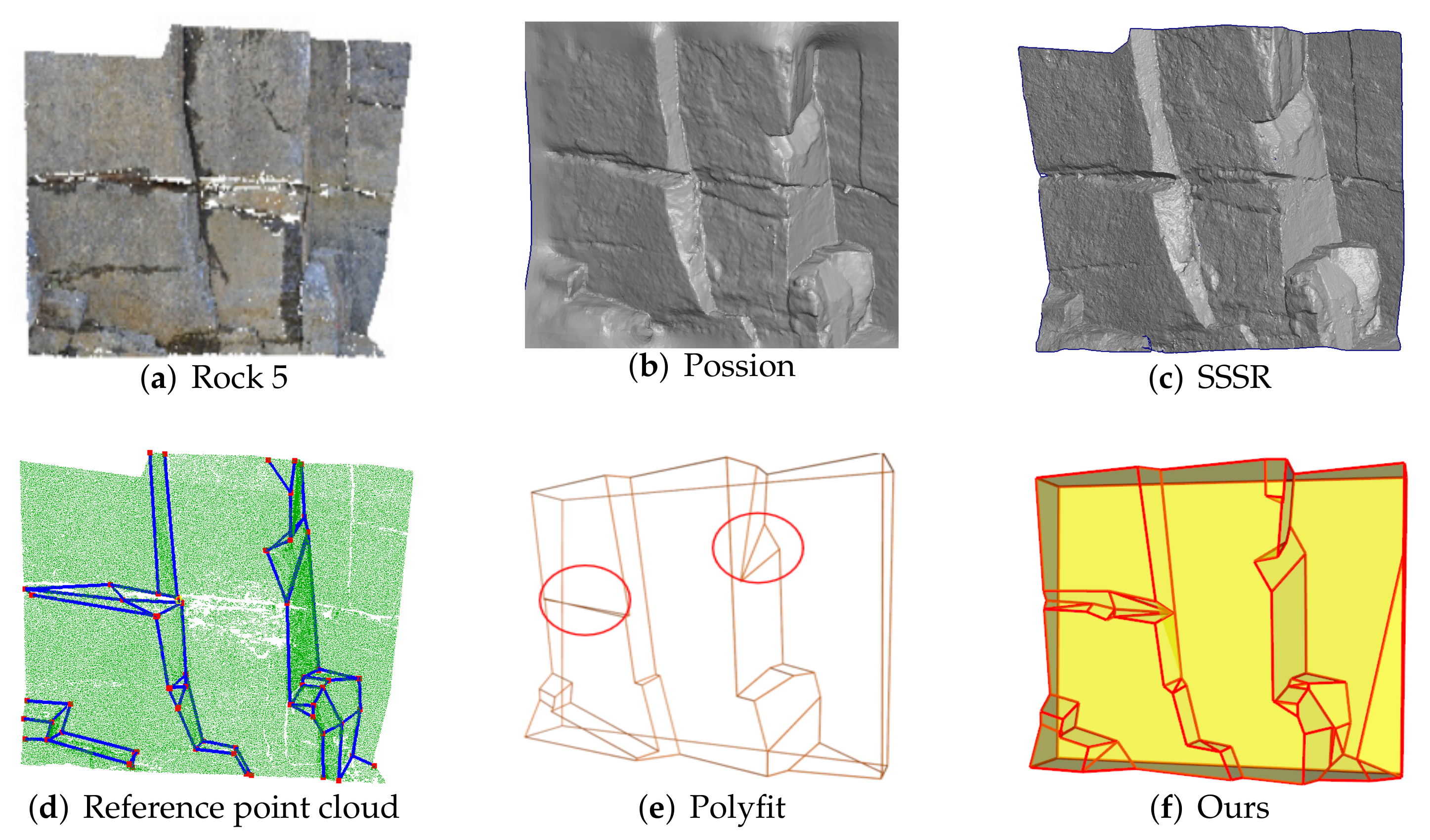
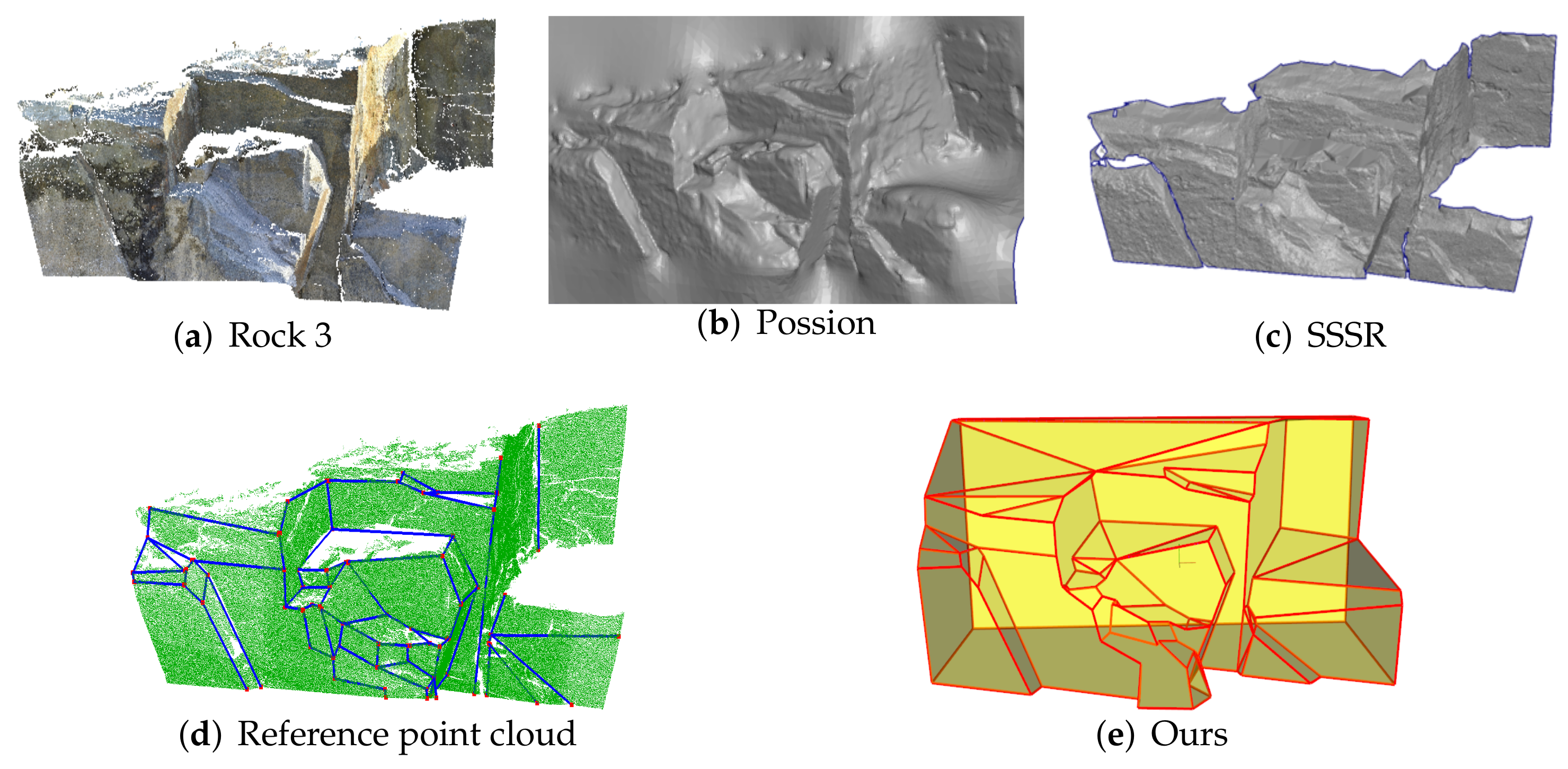
In this section, we will show the reconstruction results of multiple sets of data. In order to better reflect the performance advantages of this method, we have selected three methods for comparative experiments. Among them, Poisson [12] and SSSR [13] are two dense surface reconstruction methods. The former is widely used in a large number of tasks related to 3D reconstruction, while the latter has higher reconstruction efficiency and good reconstruction accuracy. In addition, since most of the current lightweight surface reconstruction methods are aimed at artificial target data, we choose Polyfit with strong generalization ability as the comparison method of lightweight surface reconstruction. Meanwhile, two sets of rock mass data were used for comparative experiments. Relatively speaking, Rock 5 has better data quality and simpler surface structure, while Rock 3 has poor data quality, and contains some smaller structural surfaces and transition surfaces.

Moreover, in order to better evaluate the results of lightweight reconstruction, we have marked the clear structure information contained in Rock 3 and Rock 5. It should be noted that the marking results are jointly completed by four researchers in the geotechnical field and computer vision field, and refer to the detection results of various plane detection methods, so as to make the topology contained in the marking results as accurate as possible. In this paper, we use topological accuracy as the main index to evaluate the results of lightweight reconstruction. The calculation method of topology accuracy is as follows. Using all corners in the reference point cloud to search the corresponding points (the nearest point within a certain range) in the reconstruction results. If the two endpoints of a line segment in the reference point cloud both have points corresponding to them in the reconstruction results, and the corresponding points have the same connection relationship, the topology is considered to be matched. Topology accuracy is obtained by calculating the ratio of the number of matching topologies to the total number of topologies. It should be noted that the topological accuracy is only for the lightweight surface reconstruction method. In addition, the data compression ratio is the ratio of the number of points in the original point cloud to the number of points in the model. The reconstruction results of Rock 5 and Rock 3 obtained by each method are shown in Figure 15 and Figure 16. Table 6 summarizes information about reconstruction.

Figure 15. Reconstruction results of Rock 5.

Figure 16. Reconstruction results of Rock 3.

Table 6. Details of Rock 5 and Rock 3 reconstruction results.

Data	Method	Number of Points	Number of Faces	Data Compression Ratio	Is it Closed	Time Consuming	Topological Accuracy
Rock 5	Possion	69,755	139,133	1.994	No	4.5 s	✕
	SSSR	112,006	223,557	1.004	No	2.8 s	✕
	Polyfit	45	26	2499.222	Yes	14.7 s	47%
	Ours	76	52	1479.801	Yes	12.44 s	82.3%
Rock 3	Possion	45,828	91,430	6.821	No	6.8 s	✕
	SSSR	310,740	620,376	1.006	No	3.6 s	✕
	Polyfit	✕	✕	✕	✕	✕	✕
	Ours	71	90	4403.647	Yes	17.83 s	82.6%

In general, dense reconstruction methods show high efficiency and the ability to preserve all details. However, considering that the purpose of surface reconstruction of the rock mass is to provide input data for engineering calculations and related simulation tasks, weak texture information does not need to be preserved in the final reconstruction results. While the dense reconstruction algorithm obviously does not have the ability to effectively filter the texture information and retain the effective main structure. It is noteworthy that, during the collection of the rock-mass point cloud, there is only one side of the surface information that can be obtained in many cases. The current dense reconstruction methods and some methods to simplify the dense mesh [37,38] usually do not consider reconstructing an open point cloud into a watertight model, which further explains why the models reconstructed by these methods are not suitable for some numerical simulation methods (key blocks).

The lightweight reconstruction method has good data compression ability, can effectively filter the texture information, and can generate a watertight model, which is more suitable for the reconstruction task in engineering calculation. By observing the reconstruction results of Rock 5, it can be found that Polyfit is also an effective solution for areas with simple structure and good data quality. However, in some concave regions, Polyfit may lead to inaccurate reconstruction results. The loss of information caused by occlusion makes Polyfit ineffective in the reconstruction of concave areas, which leads to a significant reduction in topology accuracy (47%). Unlike Rock 5, Polyfit cannot effectively reconstruct Rock 3, mainly for the following two reasons. First, the data quality of Rock 3 is much worse. After performing plane extension and cutting, effective cutting (even wrong cutting) can not be found in a large number of information missing areas, resulting in the collapse of the program. In fact, the inability to deal with data corruption caused by various reasons is the main problem encountered by Polyfit and its improved algorithm [33]. Second, when the structural plane set contains a large number of structural planes or transition planes with similar parameters, a large number of cutting planes will be generated in the process of global expansion, resulting in a sharp increase in the computational cost.

The method proposed in this paper can effectively filter the texture information in the point cloud under the premise of ensuring high topological accuracy, and generate a watertight model that can be directly used in engineering calculations and numerical simulations. Furthermore, the method has significant advantages in handling highly corrupted data.

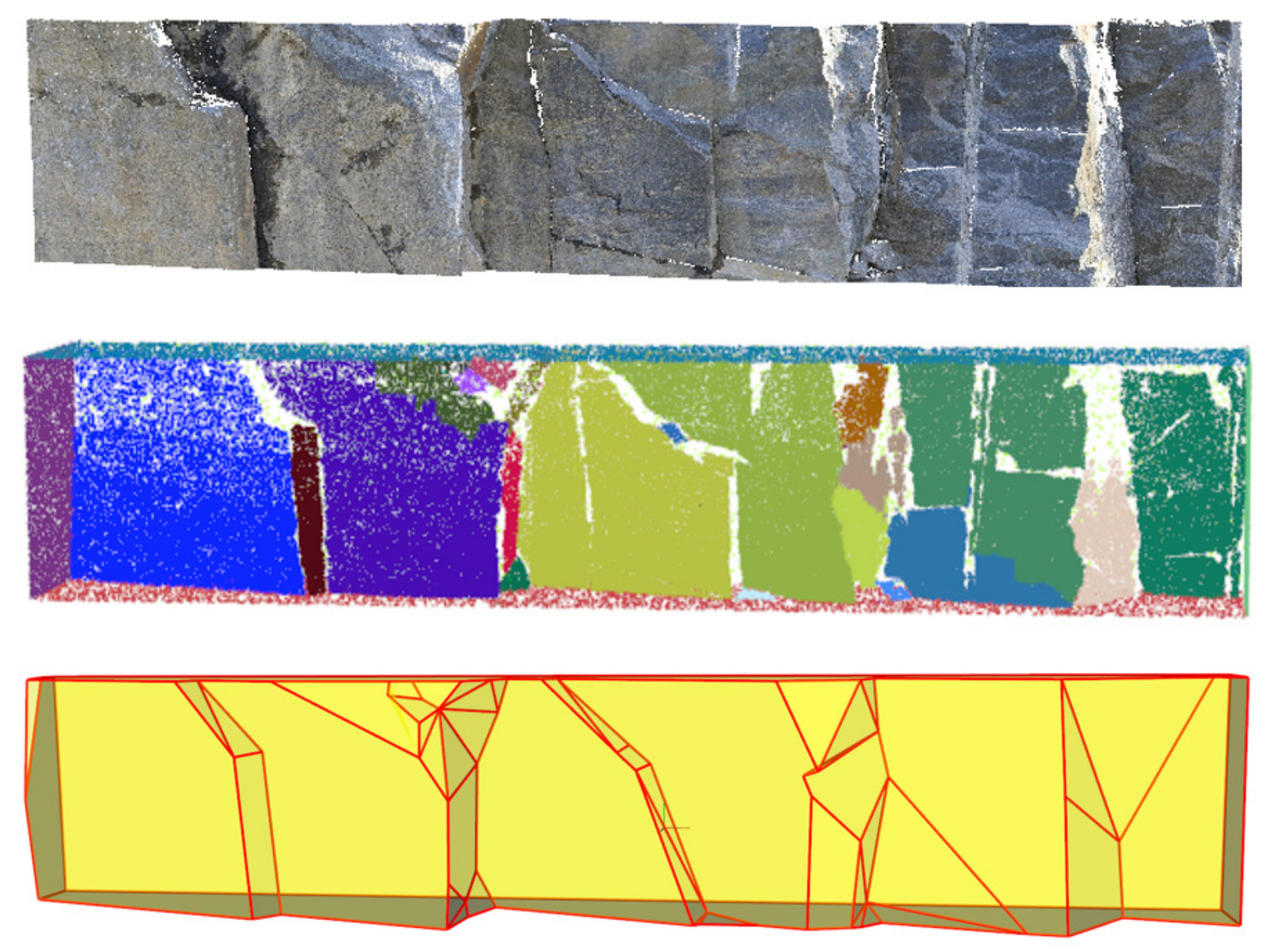
In addition, in order to show the performance of the method more comprehensively, we provide the reconstruction results of the other two groups of data. The reconstruction result of Rock 6 is shown in Figure 17. When dealing with the rock mass data with large size or including multiple groups of continuous structural planes (Rock 6), large region growth parameters should be used to avoid too many collision problems ($gro{w}_{dis}=0.21$, $gro{w}_{ang}={16}^{\circ }$). Therefore, compared with other reconstruction results, the reconstruction result of Rock 6 may lose some structural information. In fact, if more accurate reconstruction results are needed, it is suggested to reconstruct large-scale complex data in segments.

Figure 17. Reconstruction results of Rock 6.

Rock 7 is a set of data from the mountain dataset of Wuhan University. Unlike rock mass data, mountain data usually do not contain a large number of smooth structural planes. For mountain data with rough surfaces, it is still recommended to use larger region growing parameters for reconstruction to reduce the complexity of the model ($gro{w}_{dis}=0.23$, $gro{w}_{ang}={18}^{\circ }$). The reconstruction result of Rock 7 is shown in Figure 18. By observing the input data and reconstruction results of Rock 7, it can be found that the obvious structural information (surface structure changes) in the input data can be effectively extracted and finally presented in the model, which proves the effectiveness of this method in the mountain dataset. The time consumption of all rock mass data reconstruction and the basic information of each model are shown in Table 7.

Figure 18. Reconstruction results of Rock 7.

Table 7. Reconstruction information of all rocks.

Data	Segmentation Time	Reconstruction Time	Structural Planes	Model Planes
Rock 1	$9.47$ s	$11.4$ s	32	64
Rock 2	$3.27$ s	$5.13$ s	12	28
Rock 3	$8.31$ s	$9.52$ s	32	63
Rock 4	$3.51$ s	$7.76$ s	15	43
Rock 5	$6.32$ s	$6.12$ s	24	71
Rock 6	$8.02$ s	$9.27$ s	20	54
Rock 7	$5.11$ s	$4.12$ s	12	26

4.6. Application

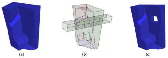
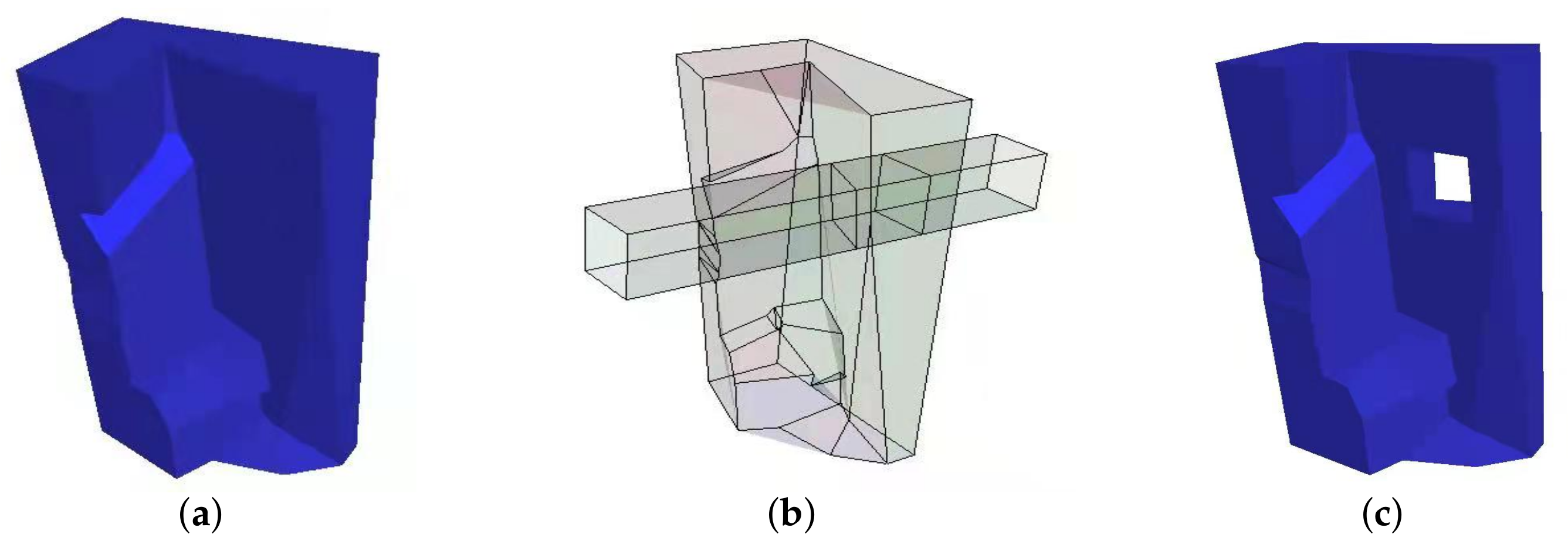
The reconstructed model can be used in the numerical simulation of engineering calculations, such as slopes and tunnels. In the actual engineering calculation, the model will be used as the input data of numerical simulation together with the actual engineering or geological conditions. Figure 19 shows a simple model example of adding a tunnel to the rock mass. After adding the size information of the tunnel to the rock mass model, the initial closed model will be further cut to form a new closed block. This information can be used in the rationality calculation of tunnel design. In addition, by adding fault information to the rock mass model and further dividing the rock mass model, the whole block can be cut into several closed sub-blocks (this is why the generated rock mass model needs to be watertight), then the stability of the rock mass can be analyzed by using block theory and discontinuous theory. In fact, when large-scale rock engineering calculation is carried out, minor changes in rock surface structure (surface texture and slight concave–convex changes) are usually not considered. On the contrary, too complex structures will make the subsequent further segmentation process difficult to perform. Therefore, in the above applications, a closed and concise numerical model of rock mass is essential.

Figure 19. Example of adding tunnel information to rock mass model (a) Input model. (b) Add tunnel information. (c) Block after cutting.

5. Conclusions

This paper focuses on the efficient lightweight surface reconstruction method of rock mass point cloud. Different from the man-made target, a large amount of texture information and inevitable data loss on the surface of rock mass are two difficulties to be solved during rock-mass point cloud surface reconstruction. Considering the above factors, this paper proposes a lightweight surface reconstruction method, which can generate a rock-mass numerical model with concise and accurate surface structure information. The generated model can be directly used for numerical simulation.

In this paper, seven groups of rock mass data are used to verify the proposed algorithm, and sufficient comparative experiments are carried out. This method can realize efficient lightweight surface reconstruction of rock-mass point cloud within high topological accuracy.It is worth mentioning that we effectively solve the collision problem caused by accumulated errors during surface reconstruction. In addition, we have analyzed and tested the problem of data corruption caused by many situations to ensure the effectiveness of the algorithm in dealing with highly corrupted data.

The proposed method constructs a watertight rock mass model by adding a rectangular bounding box, which may result in a certain number of redundant faces in the generated model. These redundant surfaces will not affect the numerical simulation but will bring some visual differences. In addition, when the outer boundary of the input data is too irregular, it becomes more difficult to add connectivity information to the bounding box. Therefore, the related problems involving bounding boxes can be further studied. At the same time, in order to avoid too many iterations during adaptive adjustment, appropriate human intervention is still necessary when dealing with some complex data. Finally, when this method deals with large-scale rock mass data, it is difficult to obtain high-precision reconstruction results. Therefore, how to reasonably decompose the large-scale reconstruction task into several sub-tasks and combine multiple sub-models to obtain high-precision reconstruction results deserves further study.

References

- Bouzas, V.; Ledoux, H.; Nan, L. Structure-aware building mesh polygonization. ISPRS-J. Photogramm. Remote Sens. 2020, 167, 432–442. [Google Scholar] [CrossRef] [Scilit]
- Cui, Y.; Li, Q.; Yang, B. Automatic 3-d reconstruction of indoor environment with mobile laser scanning point clouds. IEEE J. Sel. Top. Appl. Earth Observ. Remote Sens. 2019, 99, 1–14. [Google Scholar] [CrossRef] [Scilit]
- Turner, E.; Cheng, P.; Zakhor, A. Fast, automated, scalable generation of textured 3d models of indoor environments. IEEE J. Sel. Top. Appl. Earth Observ. Remote Sens. 2015, 9, 409–421. [Google Scholar] [CrossRef] [Scilit]
- Nan, L.; Wonka, P. Polyfit: Polygonal surface reconstruction from point clouds. In Proceedings of the 2017 IEEE International Conference on Computer Vision (ICCV), Venice, Italy, 22–29 October 2017; pp. 2372–2380. [Google Scholar]
- Li, Y.; Wu, X.; Chrysathou, Y. Globfit: Consistently fitting primitives by discovering global relations. ACM Trans. Graph. 2011, 30, 1–12. [Google Scholar]
- Ikehata, S.; Yang, H.; Furukawa, Y. Structured indoor modeling. In Proceedings of the 2015 IEEE International Conference on Computer Vision (ICCV), Santiago, Chile, 7–13 December 2015; pp. 1323–1331. [Google Scholar]
- Zhou, Q.; Neumann, U. 2.5d dual contouring: A robust approach to creating building models from aerial lidar point clouds. In Proceedings of the 11th European Conference on Computer Vision (ECCV), Heraklion, Greece, 5–11 September 2010; pp. 115–128. [Google Scholar]
- Li, M.; Nan, L. Feature-preserving 3D mesh simplification for urban buildings. ISPRS-J. Photogramm. Remote Sens. 2021, 173, 135–150. [Google Scholar] [CrossRef] [Scilit]
- Blackwood, R. Block theory and its application to rock engineering. Eng. Geol. 1988, 26, 103–105. [Google Scholar] [CrossRef] [Scilit]
- Shi, G. Discontinuous deformation analysis: A new numerical model for the statics and dynamics of deformable block structures. Eng. Comput. 1992, 9, 157–168. [Google Scholar] [CrossRef] [Scilit]
- He, L.; Zhao, Z. Development of three-dimensional numerical manifold method for jointed rock slope stability analysis. Int. J. Rock Mech. Min. Sci. 2012, 64, 22–35. [Google Scholar] [CrossRef] [Scilit]
- Kazhdan, M.; Bolitho, M.; Hoppe, H. Poisson surface reconstruction. Symp. Geom. Process. 2006, 7, 61–70. [Google Scholar]
- Boltcheva, D.; Levy, B. Simple and Scalable Surface Reconstruction; Research Report; LORIA—Université de Lorraine, INRIA Nancy: Villers-lès-Nancy, France, 2016; Available online: https://hal.archives-ouvertes.fr/hal-01349023/ (accessed on 30 December 2021).
- Hoppe, H. Surface reconstruction from unorganized points. ACM Trans. Graph. 1992, 26, 71–78. [Google Scholar]
- Curless, B.; Levoy, M. Surface reconstruction from unorganized points. In Proceedings of the 23rd Annual Conference on COMPUTER Graphics and Interactive Techniques, New York, NY, USA, 23–28 July 1996; pp. 303–312. [Google Scholar]
- Fischler, M.; Bolle, R. Random sample consensus: A paradigm for model fitting with applications to image analysis and automated cartography. Commun. ACM 1981, 24, 381–395. [Google Scholar] [CrossRef] [Scilit]
- Riquelme, A.; Abellan, A.; Jaboyedoff, M. A new approach for semi-automatic rock mass joints recognition from 3d point clouds. Comput. Geosci. 2014, 68, 35–52. [Google Scholar] [CrossRef] [Scilit]
- Leng, X.; Xiao, J.; Wang, Y. A multi-scale plane-detection method based on the hough transform and region growing. Photogramm. Rec. 2016, 31, 166–192. [Google Scholar] [CrossRef] [Scilit]
- Liu, L.; Xiao, J.; Wang, Y. Major orientation estimation-based rock surface extraction for 3d rock-mass point clouds. Remote Sens. 2019, 11, 635. [Google Scholar] [CrossRef] [Scilit]
- Hu, L.; Xiao, J.; Wang, Y. Efficient and automatic plane detection approach for 3-D rock mass point clouds. Multimed. Tools Appl. 2019, 1, 1–26. [Google Scholar] [CrossRef] [Scilit]
- Jiang, H.; Xiao, J. A linear approach to matching cuboids in rgbd images. In Proceedings of the 2013 IEEE Conference on Computer Vision and Pattern Recognition, Washington, DC, USA, 23–28 June 2013; pp. 2171–2178. [Google Scholar]
- Li, M.; Nan, L.; Smith, N. Reconstructing building mass models from uav images. Comput. Graph. 2016, 54, 84–93. [Google Scholar] [CrossRef] [Scilit]
- Li, M.; Wonka, P.; Nan, L. Manhattan-world urban reconstruction from point clouds. In Proceedings of the European Conference on Computer Vision, Amsterdam, The Netherlands, 8–16 October 2016; pp. 54–69. [Google Scholar]
- Huang, J.; Jiang, T.; Shi, Z. L1-based construction of polycube maps from complex shapes. Trans. Graph. 2014, 33, 1–11. [Google Scholar]
- Vanegas, C.; Aliaga, D.; Benes, B. Automatic extraction of manhattan-world building masses from 3d laser range scans. IEEE Trans. Vis. Comput. Graph. 2012, 18, 1627–1637. [Google Scholar] [CrossRef] [Scilit] [PubMed]
- Schindler, F.; Wörstner, W.; Frahm, J. Classification and reconstruction of surfaces from point clouds of man-made objects. In Proceedings of the 2011 IEEE International Conference on Computer Vision, Barcelona, Spain, 6–13 November 2011; pp. 257–263. [Google Scholar]
- Arikan, M.; Schwarzler, M.; Flory, S. O-snap: Optimization-based snapping for modeling architecture. ACM Trans. Graph. 2013, 32, 1–15. [Google Scholar] [CrossRef] [Scilit]
- Lafarge, F.; Alliez, P. Surface reconstruction through point set structuring. Comput. Graph. Forum. 2013, 32, 225–254. [Google Scholar] [CrossRef] [Scilit]
- Holzmann, T.; Maurer, M.; Bischof, H. Semantically aware urban 3d reconstruction with plane-based regularization. In Proceedings of the 2018 European Conference on Computer Vision, Munich, Germany, 8–14 September 2018; pp. 487–503. [Google Scholar]
- Chauve, A.; Labatut, P.; Pons, J. Robust piecewise-planar 3d reconstruction and completion from large-scale unstructured point data. In Proceedings of the 2010 IEEE Conference on Computer Vision and Pattern Recognition, San Francisco, CA, USA, 13–18 June 2010; pp. 1261–1268. [Google Scholar]
- Verdie, Y.; Lafarge, F.; Alliez, P. Lod generation for urban scenes. ACM Trans. Graph. 2015, 34, 1–14. [Google Scholar] [CrossRef] [Scilit]
- Mura, C.; Mattauschand, O.; Pajarola, R. Piecewise-planar reconstruction of multi-room interiors with arbitrary wall arrangements. Comput. Graph. Forum. 2016, 35, 179–188. [Google Scholar] [CrossRef] [Scilit]
- Bauchetand, J.; Lafarge, F. Kinetic shape reconstruction. ACM Trans. Graph. 2020, 38, 1–14. [Google Scholar] [CrossRef] [Scilit]
- Rusu, R.; Cousins, S. 3d is here: Point cloud library(pcl). In Proceedings of the 2011 IEEE International Conference on Robotics and Automation, Shanghai, China, 9–13 May 2011; pp. 1–4. [Google Scholar]
- Lato, M.; Bevan, B.; Kemeny, J. Rock bench: Establishing a common repository and standards for assessing rockmass characteristics using lidar and photogrammetry. Comput. Geosci. 2013, 50, 106–114. [Google Scholar] [CrossRef] [Scilit]
- Dong, Z.; Yang, B. A novel binary shape context for 3d local surface description. ISPRS J. Photogramm. Remote Sens. 2017, 130, 431–452. [Google Scholar] [CrossRef] [Scilit]
- Salinas, D.; Lafarge, F.; Alliez, P. Structure-aware mesh decimation. Comput. Graph. Forum. 2015, 34, 211–227. [Google Scholar] [CrossRef] [Scilit]
- Chen, D.; Sitthi, P. Computing and fabricating multiplanar models. Comput. Graph. Forum. 2015, 32, 305–315. [Google Scholar] [CrossRef] [Scilit]
Publisher’s Note: MDPI stays neutral with regard to jurisdictional claims in published maps and institutional affiliations. |
© 2022 by the authors. Licensee MDPI, Basel, Switzerland. This article is an open access article distributed under the terms and conditions of the Creative Commons Attribution (CC BY) license (https://creativecommons.org/licenses/by/4.0/).