Abstract
Even though research has shown that the spectral parameters of yellow-edge, red-edge and NIR (near-infrared) shoulder wavelength regions are able to estimate green cover and leaf area index (LAI), a large amount of dead materials in grasslands challenges the accuracy of their estimation using hyperspectral remote sensing. However, the exact impact of dead vegetation cover on these spectral parameters remains unclear. Therefore, we evaluated the influences of dead materials on the spectral parameters in the wavelength regions of yellow-edge, red-edge and NIR shoulder by comparing normalized difference vegetation indices (NDVI) including the common red valley at 670 nm and NDVI using the red valley extracted by a new statistical method. This method, based on the concept of segmented linear regression, was developed to extract the spectral parameters and calculate NDVI automatically from the hyper-spectra. To fully understand the impact of dead cover on the spectral parameters (i.e., consider full coverage combinations of green vegetation, dead materials and bare soil), both in situ measured and simulated hyper-spectra were analyzed. The impact of dead cover on LAI estimation by those spectral parameters and NDVI were also evaluated. The results show that: (i) without considering the influence of bare soil, dead materials decreases the slope of red-edge, the slope of NIR shoulder and NDVI, while dead materials increases the slope of yellow-edge; (ii) the spectral characteristics of red valley disappear when dead cover exceeds 67%; (iii) large amount of dead materials also result in a blue shift of the red-edge position; (iv) accurate extraction of the red valley position enhances LAI estimation and reduces the influences of dead materials using hyperspectral NDVI; (v) the accuracy of LAI estimation using the slope of yellow-edge, the slope of red-edge, red-edge position and NDVI significantly drops when dead cover exceeds 72.3–74.5% (variation among indices).
1. Introduction
Dead material (non-photosynthetic vegetation: NPV; including standing dead tissue and litter) is a prominent component of grasslands, especially in relatively undisturbed swards in arid or semi-arid climate regions [1]. Dead material, a vital transfer phase of energy, carbon and nutrition from plants to soil [2], has large impact on water infiltration [3], evaporation [4], species composition [5] and grassland productivity [6]. However, too much accumulation of NPV can reduce grassland productivity because dense litter layers impede seed germination [7] and standing dead plants compete for space with green vegetation [1].
In grasslands, the ability of remote sensing to evaluate vegetation cover, biomass and productivity has been demonstrated in many studies [8,9,10,11,12,13,14,15,16,17]. For hyperspectral remote sensing, the spectral characteristics of green, red, red-edge and near-infrared (NIR) regions are sensitive to grassland vegetation growth [18,19] and are widely used in monitoring green cover [9], leaf area index (LAI) [20], biomass [21] and ecological characteristics [22]. The parameters of yellow-edge [23], red-edge [24], NIR shoulder [20] and various vegetation indices (e.g., the most popular vegetation index [25]: NDVI (Normalized difference vegetation Index)) [20] indicate the spectral characteristics of the four wavelength regions. However, the estimation accuracy of LAI or green cover is unstable in grasslands, especially the grassland with large amounts of dead materials [25]. Previous studies also discovered that total biomass has a positive relationship with NDVI when dead cover is low but has no significant relationship with NDVI when dead cover is large [1]. Therefore, it is significant to explore how dead materials influence the spectral parameters of the four wavelength regions of green, red, red-edge and NIR shoulder (i.e., those spectral parameters are well documented to be sensitive to grassland growth [8,9,10,11,12,13,14,15,16,17]).
Red-edge parameters, including red-edge position (REP), red-edge amplitude (REA) and red-edge area [26,27], are the most popular indices for detecting the biophysical characteristics of vegetation growth, including chlorophyll content [27], LAI [24], biomass [28], nitrogen status [29], growth stage [30,31] and vegetation response to stress and disturbance [27,32,33]. Red-edge parameters also enhance the separation among vegetation types [28,34] and different ground features [28]. The satellite (RapidEye, WorldView-2/3, Sentinel-2 and Gaofen-6) imagery, designed with red-edge bands, is helpful to improve classification accuracy and enhance LAI estimation by migrating saturation issues [28,35,36,37,38]. Although, comparing to vegetation indices, red-edge parameters are less sensitive to the changes in specific biophysical factors (vegetation type, canopy structure and soil cover) and environment conditions (site condition, atmospheric effects, irradiance and solar zenith angle) [29,39]. Wei et al.’s research indicates that the red-edge parameters are affected by the underlying surface in arid grasslands [23]. However, it remains unclear exactly how dead materials, a large component of native grasslands, influence red-edge parameters. In addition to red-edge and yellow-edge parameters [29], the NIR shoulder [20] and red absorption valley [33] are rarely used in vegetation monitoring.
Therefore, the aim of this study is to explore the impact of dead materials on yellow-edge parameters, red absorption valley, red-edge parameters and NIR shoulder, as well as NDVI, for a better understanding of grassland monitoring using spectral signals in the green, red, red-edge and NIR wavelength regions. Our objectives were to: (1) develop a mathematic method to extract spectral parameters of yellow-edge, red valley, red-edge and NIR shoulder, (2) explore the impact of dead materials on those spectral parameters and hyperspectral NDVI (i.e., including NDVI calculated by the common red valley at 670 nm and the accurate red valley extracted by the developed method), and (3) to assess how NPV influences the accuracy of LAI estimation by the spectral parameters or the two types hyperspectral NDVI in grassland ecosystems.
2. Materials and Methods
2.1. Study Area
Our study was conducted in the West Block of Grasslands National Park (GNP) and the surrounding pastures (Figure 1a) in the mixed prairie region, Canada [40]. Grasslands in GNP have large amount of dead material accumulation because it has been managed under low disturbance since it was first designated as a national park in 1984 [41]. The climate of GNP is characterized as a semi-arid climate, with a 3.4 °C annual mean temperature and 340 mm annual precipitation [25]. The heterogeneity of dead cover in GNP compared to surrounding pastures with greater disturbance provided a meaningful contrast, which makes GNP a suitable study area for this research. However, due to the nature of mixed-grass prairie, areas of high green cover [1] are absent (Table 1), preventing a complete range of spectral parameters in the yellow-edge, red valley, red-edge and NIR shoulder regions as dead cover ranged from 0–100%. Therefore, we added a secondary study area, a subalpine meadow in Wuyishan National Park (WNP; Figure 1b) in the subtropical monsoon humid climate region of China [42]. Due to high precipitation (approximate 2800 mm per year) and warm temperature (a 9 °C annual mean temperature) [43], this subalpine meadow has high green vegetation cover during the peak growing season (Table 1). The grasslands in GNP are dominated by western wheatgrass (Agropyron smithii Rydb.), northern wheatgrass (Agropyron dasystachym), needle-and-thread grass (Stipa comata Trin. & Rupr.) and blue grama grass (Bouteloua gracilis (HBK) Lang. ex Steud.) [25]; the subalpine meadow in WNP is dominated by Miscanthus sinensis, Deyeuxia arundinacea and Molinia japonica [42].
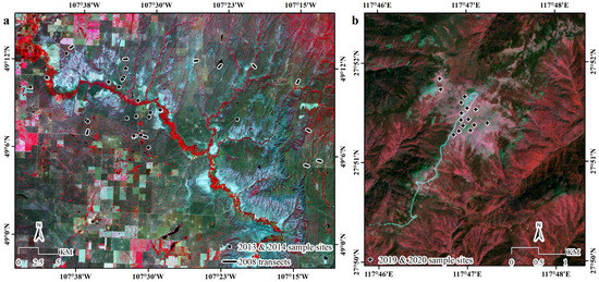
Figure 1.
Study area: (a) Grasslands National Park (GNP) and the surrounding pastures (the background image is a Sentinel-2 scene acquired on 17 July 2017, with a standard false color composition (near-infrared, red and green band in red, green, and blue channel, respectively)); (b) subalpine meadow in Wuyishan National Park (the background image is a Sentinel-2 scene acquired on 19 September 2019, with a standard false color composition).

Table 1.
Description of the field collected in both Grasslands National Park (GNP) and Wuyishan National Park (WNP).
2.2. Data Collection
Fieldwork in GNP and the surrounding pastures was conducted during peak growing season (late June to early July) of 2008, 2013 and 2014. Twelve transects in 2008, 9 sites in 2013 and 12 sites in 2014 were sampled based on a stratified random design and accessibility (Figure 1a). Twenty quadrats (i.e., size: 50 m × 50 m) were set up along a 100 m × 100 m plot with 10 m interval at each site, while 128 quadrats (i.e., size: 50 m × 50 m) were set up along each transect with 3 m interval (see the detailed quadrat design in the reference [1]). Nine sites in 2019 and 12 sites in 2020 were selected based on the stratified random design in the subalpine meadow in WNP (Figure 1b). The quadrat design was similar to the sites sampled in GNP.
The percentage cover of green grass, forb, shrub, standing dead, litter, lichen, moss, bare soil and rock were estimated by observation in each quadrat. For each quadrat, the hyperspectral reflectance was measured by analytical spectral devices (ASD) field-portable FieldSpec®Pro Spectroradiometer (Malvern Panalytical Ltd., Malvern, UK) (wavelength from 350 nm to 2500 nm) and ASD FieldSpec®Handheld 2 Spectroradiometer (wavelength from 325 nm to 1075 nm) for GNP and WNP, respectively. The hyperspectral reflectance was collected on sunny days with clear skies between 10 a.m. and 2 p.m. (i.e., the optimal time period for taking reflectance measurement is within ±2 h of local noon because the interval between the reflectance measurement is a function of the change rate of the solar elevation angle). Before collecting reflectance data, the ASD instrument was calibrated using a white reference with a time interval of 15–20 min. For each quadrat, three measurements of the reflectance were collected from one meter above the grassland canopy in a nadir view (i.e., downward facing). LAI was measured using a Li-cor LAI-2000 (LI-COR, Lincoln, NE, USA) and LAI-2200 for GNP and WNP, respectively, with one above canopy measurement in a shadow region, and six below canopy measurements within each quadrat (see the descriptive statistics of all the field collected data in Table 1).
2.3. Automatic Extraction of Spectral Parameters of Yellow-Edge, Red-Edge and NIR Shoulder
The hyperspectral data analyzed for this study covered the wavelength region of yellow-edge, red-edge ad NIR shoulder (600–900 nm). The spectral parameters of yellow-edge, red-edge and NIR shoulder are the slope of yellow-edge, red valley position, the slope of red-edge, red-edge position and the slope of NIR shoulder (Table 2). The spectral reflectance of the vegetation in the 600–900 nm region appears as three broken-lines, representing yellow-edge, red-edge and NIR shoulder (Figure 2). Previous studies reported slightly different wavelength regions of yellow-edge and red-edge (e.g., 560–640 nm [23] or 550–580 nm [29,44] for yellow-edge, and 680–760 nm [23,29], 670–780 nm [18,34,39] or 670–750 nm [44] for red-edge). Therefore, it is important to capture the accurate turning points between yellow-edge and red-edge, and between red-edge and NIR shoulder before extracting the spectral parameters in these three wavelength regions. A segmented linear relationship is a broken-line relationship with two or more straight lines joined by one or more points which are named turning points, change-points, or thresholds [1]. The segmented linear model is often used to identify thresholds or turning points in a broken-line relationship [42]. In this study, segmented linear regression was applied to capture the thresholds of wavelength for separating yellow-edge, red-edge and NIR shoulder (i.e., wavelength as an independent variable and reflectance as response variable; Figure 2) using the Segmented package in R software (R Core Team (2013). R: A language and environment for statistical computing. R Foundation for Statistical Computing, Vienna, Austria. URL http://www.R-project.org/ (assessed on 21 November 2021)). The two turning points identified by the results of segmented linear regression are R segmentation (i.e., the change-point between yellow-edge and red-edge; Table 2 and Figure 2) and NIR segmentation (i.e., the change-point between red-edge and NIR shoulder; Table 2 and Figure 2). Definitions of the yellow-edge, red-edge and NIR wavelength regions are found in Table 2 and Figure 2. Red-edge position was originally defined as the wavelength of the inflection point in the red-edge region [45], thus, red-edge position is the wavelength at the midpoint while the wavelength region of red-edge is accurately delineated. The wavelength region of the red-edge from the results of segmented linear regression occurred between R segmentation to NIR segmentation (Figure 2). Therefore, red-edge position was calculated as the average wavelength of R segmentation and NIR segmentation (Table 2). Based on the two change-points, the spectral reflectance was separated into three datasets, and a linear regression model was applied to each. The slope of each linear regression model is the slope of yellow-edge, red-edge or NIR shoulder (details in Table 2). A minimum reflectance was sought in the wavelength region from 650 nm to R segmentation to identify the red valley position (Table 2). All the steps of this automatic extraction method were written using a “for loop” in R software (see Supplementary Material).
Table 2.
Spectral parameters of yellow-edge, red-edge and NIR shoulder.
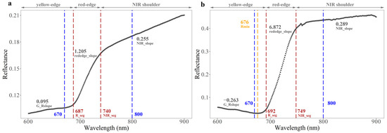
Figure 2.
Illustration of a novel method for extracting spectral parameters of yellow-edge, red-edge and NIR shoulder (G_Rslope, rededge_slope, NIR_slope, Rmin, R_seg and NIR_seg refer to the slope of yellow-edge, the slope of red-edge, the slope of NIR shoulder, red valley position, R segmentation and NIR segmentation, respectively): (a) Spectra collected in Grassland National Park (GNP), Canada (i.e., Red valley position is not detected due to the impact of dead materials); (b) Spectra measured in the subalpine meadow in Wuyishan National Park (WNP), China.
Even though the data collected in both study areas contain a variety combination of green cover, dead cover and bare soil cover, it still lacks some samples with high coverage of bare soil. For fully understanding the impact of dead cover on the spectral parameters, simulated spectral reflectance based on the lab measured spectra of bare soil, green grass and dead materials (samples were collected in GNP) based on the linear spectral mixture analysis (Equation (1)) were also analyzed in this study. In total, 231 hyper-spectra were simulated at 5% intervals of bare soil, dead and green covers in the range of 0–100% (i.e., all combination of the coverage of bare soil, dead materials and green vegetation were considered with 5% coverage interval). In addition, the analysis results of the simulated data could also be used for validating the results based on the in situ measured data.
where is the simulated hyper-spectra; , and refer to the percentage coverage of green vegetation, dead materials and bare soil, respectively; , andrefer to the lab measured hyper-spectra of green grass, dead grass and bare soil, respectively.
2.4. The Relationship between Dead Cover and the Spectral Parameters of Yellow-Edge, Red-Edge and NIR Shoulder
To fully understand how dead cover contributes to the spectral parameters of yellow-edge, red-edge and the NIR shoulder (see Table 2), the relationship between dead cover and each spectral parameter was plotted using a scatterplot with the ggplot2 library in R software. The relationship between dead cover and each spectral parameter was also analyzed using a linear model (lm() function in R software) where green and bare soil cover is set to 0%. For comparation of spectral parameters (Table 2), two type NDVI (hyperspectral NDVI (Equation (2) [46]) and NDVI using the reflectance of red valley (Equation (3)) was calculated and the relationship between dead cover and the two NDVI was analyzed.
where , and refer to the reflectance in the wavelength of 800 nm, 670 nm and red valley position (Table 2) of the field collected or simulated hyperspectral data, respectively.
To evaluate the contribution of dead cover, green cover and bare soil cover on the spectral parameters (Table 2), a multiple linear regression model was applied (i.e., the different spectral parameters as the response variable, while dead cover, green cover and bare soil cover as the explanatory variables). The column “Sum Sq” in the ANOVA table (one part of the results from linear model in R software) contains the variation of response variable (i.e., the spectral parameters) explained by each explanatory variable and the unexplained variation of the response variables due to residuals (i.e., the summary of explained variation by all three explanatory variables and unexplained variation from residuals is the variation of the response variable). Then the contribution of each explanatory variable was calculated by the percentage of the variation explained by the explanatory variable (Equation (4)).
where “Explained variation” is the contribution of each explanatory variable on the spectral parameter; “Sum Sq” is the explained variation of the response variable by each explanatory variable in the multiple linear model; “Total Sum Sq” is the total variation of the response variable.
2.5. The Imapct of NPV on LAI Estimation by the Spectral Parameters
To test the influence of NPV on the LAI estimation with spectral parameters (Table 2), a linear regression model was built for LAI independently varying the spectral parameters; a segmented linear regression (i.e., with dead cover as independent variable and the residual of the linear regression model of LAI estimation as the response variable) was applied to determine the thresholds for dead cover as the accuracy of LAI estimation changed. Finally, the correlation between the residuals and dead cover was analyzed after datasets were separated by dead cover thresholds for each model. All statistical analyses were conducted in R software.
3. Results
3.1. The Relationship of the Spectral Parameters of Yellow-Edge, Red-Edge and NIR Shoulder with Dead Cover
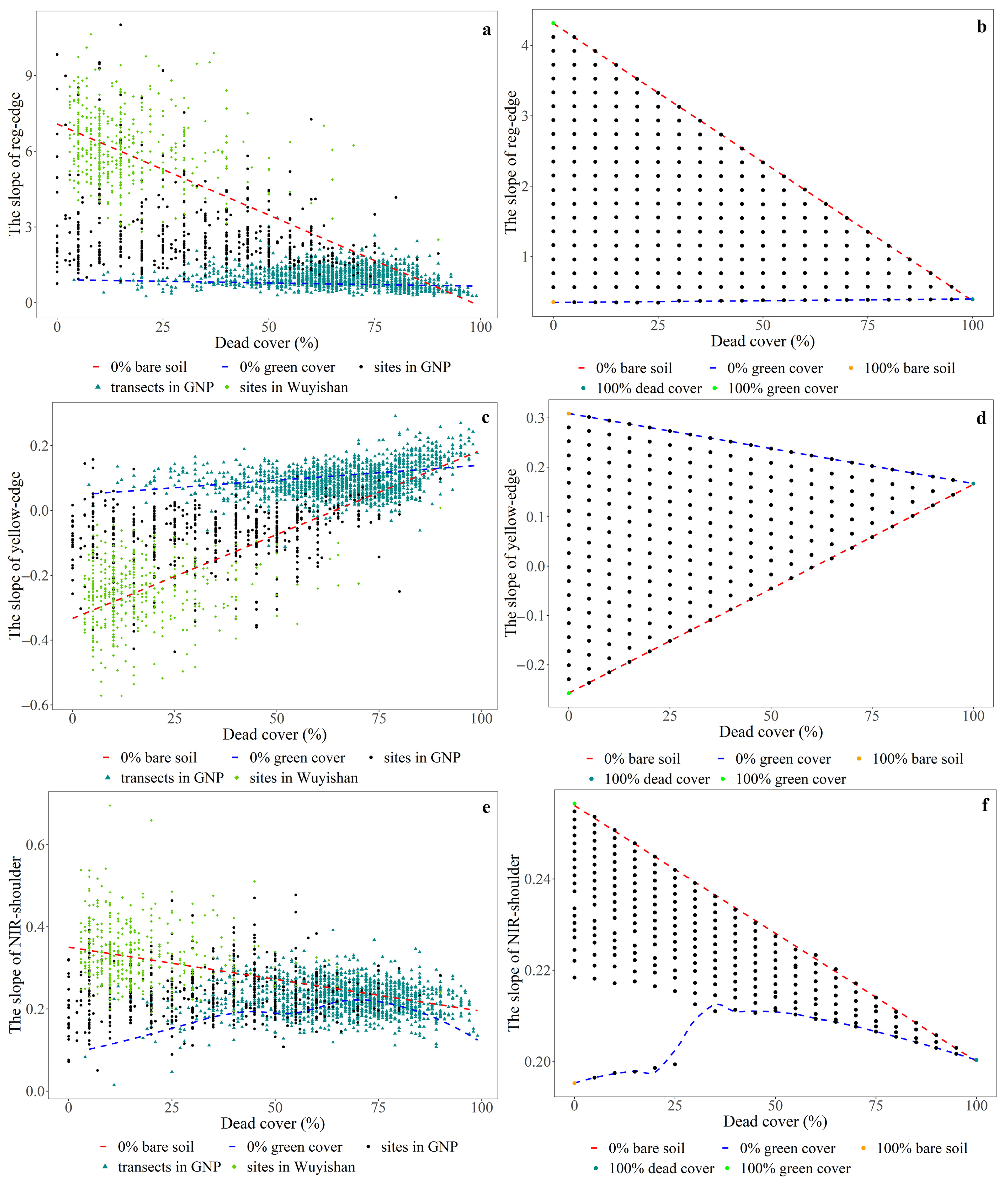
Both in situ measured and simulated spectra show similar patterns for the relationship of dead cover to red-edge slope, yellow-edge slope and the NIR shoulder slope (Figure 3). If only two components (i.e., green vegetation and dead material) occur in grasslands, dead cover has a negative linear relationship with the red-edge slope (red dashed line in Figure 3a,b; results based on field measured data: R2 = 0.763, p < 0.001, slope = −0.07, Figure 3a; results based on simulated spectra: R2 = 1, p < 0.001, slope = −0.04, Figure 3b) and slope of the NIR shoulder (red dashed line in Figure 3e,f; results based on in situ measured data: R2 = 0.389, p < 0.001, slope = −0.0016, Figure 3e; results based on simulated spectra: R2 = 0.999, p < 0.001, slope = −0.0006, Figure 3f), and a positive linear relationship with the yellow-edge slope (red dashed line in Figure 3c,d; results based on in situ measured data: R2 = 0.761, p < 0.001, slope = 0.0005, Figure 3c; results based on simulated spectra: R2 = 1, p < 0.001, slope = 0.0004, Figure 3d). With some dead cover, the increasing cover of bare soil reduces the slope of red-edge and the slope of NIR shoulder (Figure 3a,b,e,f), but increases the yellow-edge slope (Figure 3c,d). The yellow-edge slope is larger than zero when dead cover is greater than 64.19% or 60.88% based on the in situ measured or simulated spectra, respectively (i.e., the threshold is calculated based on the equation of red dashed line when the slope of yellow-edge equals to zero; Figure 3c,d). If only two components (i.e., bare soil and dead material) occur in grasslands, dead cover does not appear to have significant linear relationship with the slope of red-edge, yellow-edge or NIR shoulder (blue dash line in Figure 3). Among the slope of red-edge, yellow-edge and NIR shoulder, dead materials have highest impact on the slope of yellow-edge (0.0626%, Table 3), and lowest effects on the slope of NIR shoulder (0.003%, Table 3).
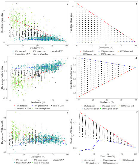
Figure 3.
Relationships between the slope of red-edge, yellow-edge, NIR shoulder and dead cover (“sites in GNP”, “transects in GNP” and “sites in Wuyishan” refer to the quadrat data collected in the sample sites in Grassland national park (GNP), in the transects in GNP, and in the sample sites in Wuyishan National Park (WNP), respectively; the red dash line refer to the linear relationship in the situation when the coverage of bare soil equals to 0%; the blue dash line means the relationship in the situation when green cover equals to 0%). The relationship between the slope of red-edge (a), yellow-edge (c), NIR shoulder (e) from in situ measured hyper-spectra and dead cover; the relationship between the slope of red-edge (b), yellow-edge (d), NIR shoulder (f) from simulated hyper-spectra and dead cover.
Table 3.
Contribution of the coverage of dead materials, green vegetation and bare soil to different spectral parameters.
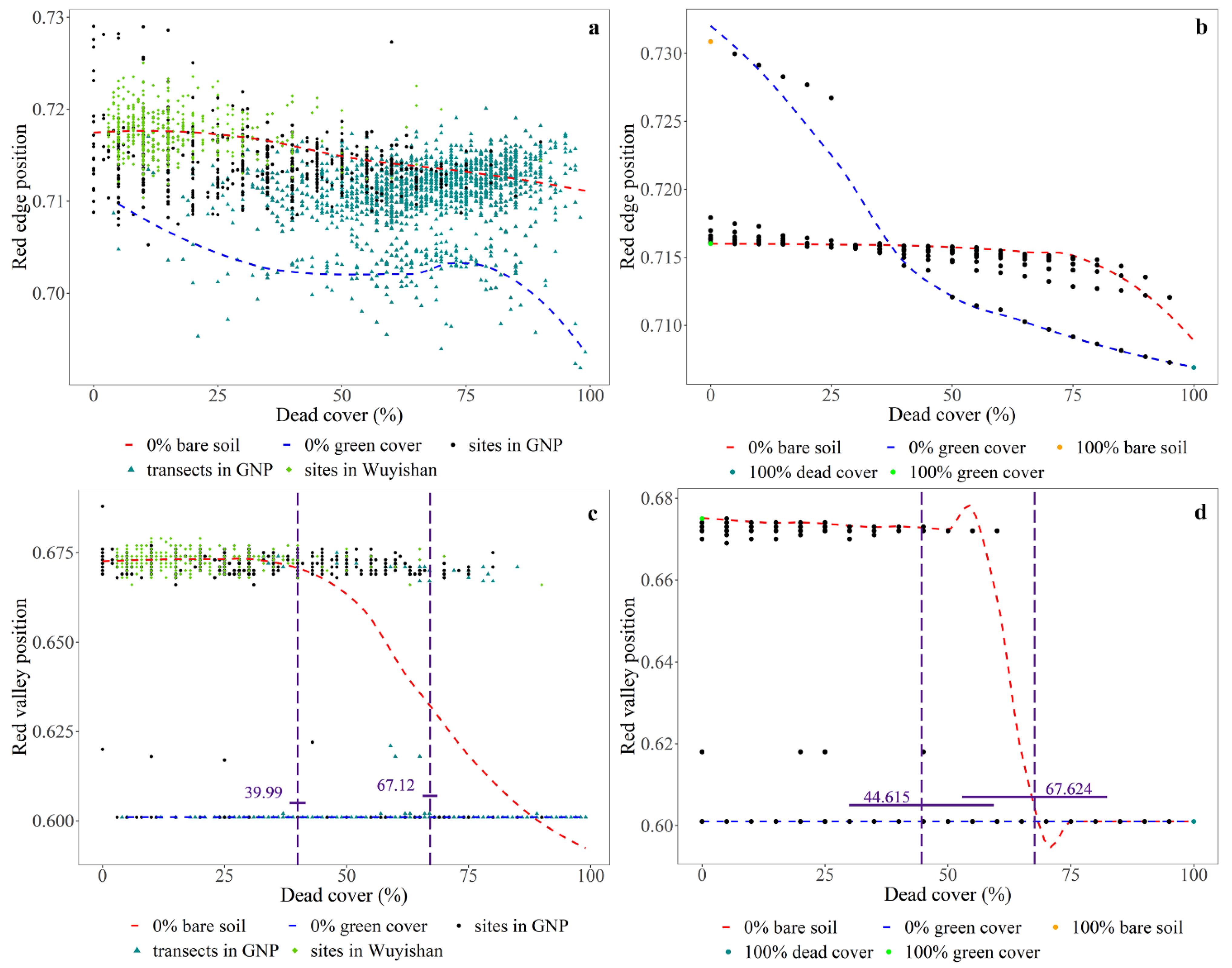
No clear red valley position appears while dead cover reaches a threshold (67.12% or 67.62% (p < 0.001) calculated by the segmented linear regression based on in situ measured spectra and simulated spectra, respectively; Figure 4c,d). High cover of bare soil would cause the same phenomena with no clear red valley position (Figure 4c,d). Comparing to bare soil (1.116%, Table 3), dead materials have slightly lower influences on red valley position (0.919%, Table 3).
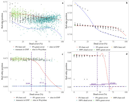
Figure 4.
The relationship between red-edge position, red valley position and dead cover (“sites in GNP”, “transects in GNP” and “sites in Wuyishan” refer to the quadrat data collected in the sample sites in Grassland national park (GNP), in the transects in GNP, and in the sample sites in Wuyishan National Park (WNP), respectively; the red dash line refer to the linear relationship in the situation when the coverage of bare soil equals to 0%; the blue dash line means the relationship in the situation when green cover equals to 0%). The relationship between red-edge position (a), red valley position (c) from field measured hyper-spectra and dead cover; the relationship between red-edge position (b), red valley position (d) from simulated hyper-spectra and dead cover.
3.2. The Relationship between NDVI and Dead Cover
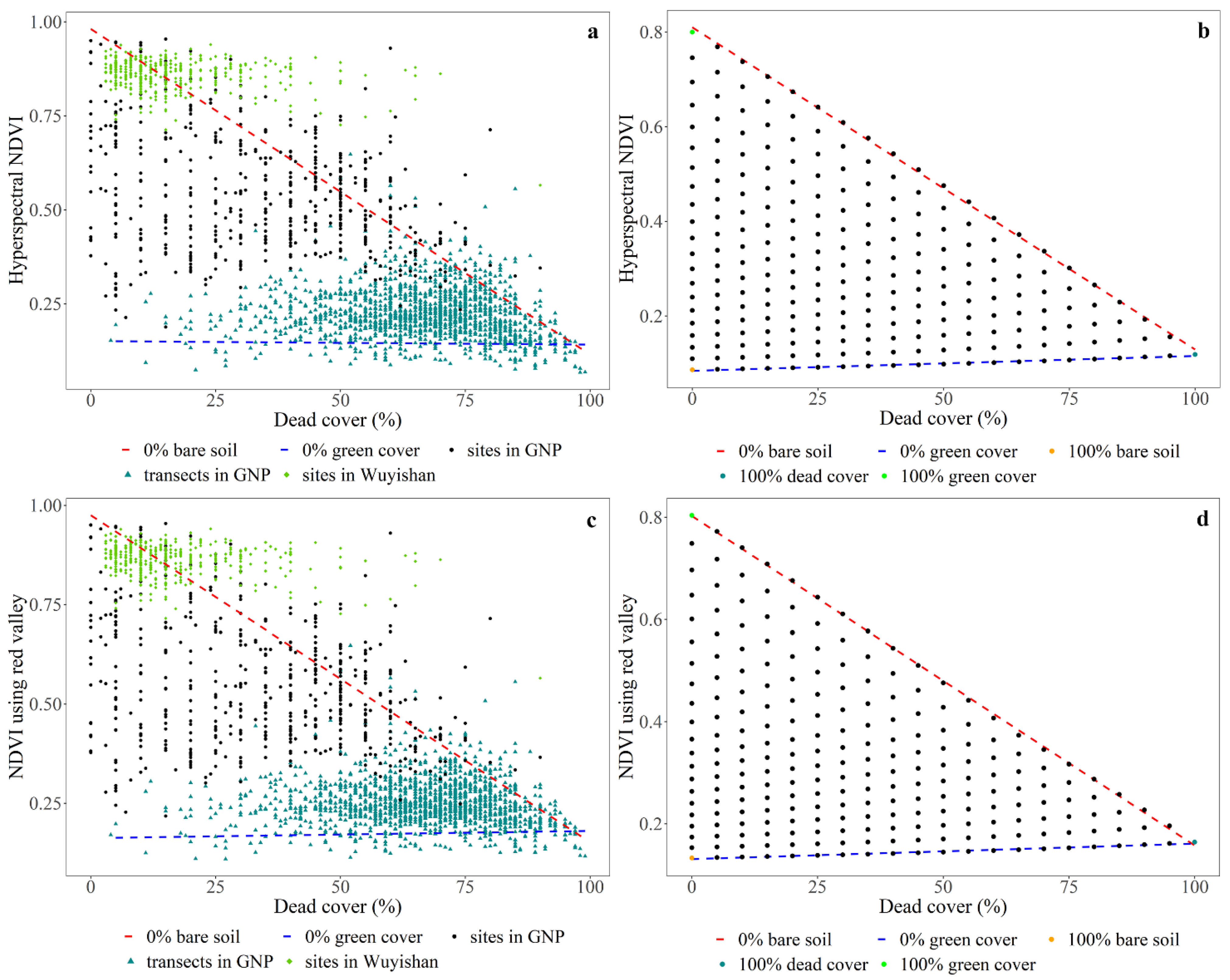
The triangular shape of the scatter plot indicates the relationship between NDVI and dead cover (Figure 5). The points in the upper part are the quadrats with less bare soil cover, while the lower points are in quadrats with higher bare soil cover (Figure 5).
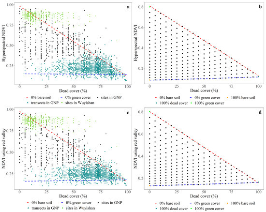
Figure 5.
The relationship between NDVI and dead cover (“sites in GNP”, “transects in GNP” and “sites in Wuyishan” refer to the quadrat data collected in the sample sites in Grassland national park (GNP), in the transects in GNP, and in the sample sites in Wuyishan National Park (WNP), respectively; the red dash line refer to the linear relationship in the situation when the coverage of bare soil equals to 0%; the blue dash line means the relationship in the situation when green cover equals to 0%): (a) The relationship between field measured hyperspectral NDVI and dead cover; (b) the relationship between simulated hyperspectral NDVI and dead cover; (c) the relationship between field measured NDVI using red valley and dead cover; (d) the relationship between simulated NDVI using red valley and dead cover.
When bare soil cover equals zero, NDVI has a negative linear relationship with dead cover (i.e., either NDVI calculated based on in situ measured spectra or simulated spectra of the same phenomena; red dashed line in Figure 5; results based on hyperspectral NDVI from in situ measured data: R2 = 0.878, p < 0.001, slope = −0.0087, Figure 5a; results based on NDVI using red valley from in situ measured data: R2 = 0.878, p < 0.001, slope = −0.0082, Figure 5c; results based on hyperspectral NDVI from the simulated spectra: R2 = 0.999, p < 0.001, slope = −0.0068, Figure 5b; results based on NDVI using red valley from the simulated spectra: R2 = 0.999, p < 0.001, slope = −0.0064, Figure 5c). However, NDVI does not have significant linear relationship with dead cover when green cover equals to 0% (i.e., only bare soil and dead materials cover the grasslands; blue dash line in Figure 5). When some dead cover occurs, NDVI decreases as bare soil cover increases (Figure 5). Comparing to hyperspectral NDVI, NDVI using red valley decreased the impact of dead materials on NDVI (Table 3; the contribution of dead materials on hyperspectral NDVI and NDVI using red valley are 0.465% and 0.389%, respectively).
3.3. Influence of Dead Cover on LAI Estimation by NDVI and Spectral Parameters of Yellow-Edge, Red-Edge and NIR Shoulder and Dead Cover
Among all indices, NDVI has the strongest linear relationship with LAI (Table 4). The hyperspectral NDVI calculated by the reflectance of red valley significantly enhances LAI estimation in grasslands (Table 4). According to both R2 and RMSE (Root Mean Square Error), LAI has a stronger relationship with the red-edge slope, followed by the yellow-edge slope and is weakest with the NIR shoulder slope (Table 4; see the correlation coefficients among different spectral parameters and LAI in Table A1; see the scatter plots with linear regression model between LAI and different spectral parameters in Figure A2). Red-edge position has a significant positive relationship with LAI (Table 4), which indicates that higher LAI would cause red-edge position shifts to higher wavelengths. The residuals of all linear regression models for LAI estimation show significant positive correlation coefficients with dead cover when dead cover exceeds a given threshold (Table 4).
Table 4.
The impact of dead cover on LAI estimation by different spectral parameters.
4. Discussion
4.1. The Influence of Dead Materials on the Spectral Parameters of Yellow-Edge, Red-Edge and NIR Shoulder
Dead cover has a fan shape relationship with the slope of red-edge, yellow-edge and NIR shoulder (Figure 3), and NDVI (Figure 5) due to the influence of bare soil. Both bare soil and dead materials result in lower slope of red-edge and NIR shoulder, higher slope of yellow-edge, and lower NDVI (Figure 3 and Figure 5). This appears to be because bare soil has similar spectral characteristics in the wavelength region of yellow-edge, red-edge and NIR shoulder [47,48]. With some dead material on the ground, the spectral parameters and NDVI varies among green cover and bare soil cover (Figure 3 and Figure 5). Normally, the grassland sampling design does not contain a full range of green vegetation, dead material and bare soil coverage, thus the statistical relationship between spectral parameters and dead cover, or between the spectral parameters and green cover is unstable [1,25]. For example, results are weaker using just field data collected in GNP (Figure A1) because GNP sites do not have full cover of green vegetation. Nevertheless, GNP contains samples with full data range of dead cover. Based on the in situ data measured in both GNP and WNP, dead materials contribute more on the slope of red-edge and NDVI than bare soil, while dead materials accounts less on the slope of yellow-edge than bare soil (Table 3).
The relationship between dead cover and the spectral parameters extracted from in situ measured hyper-spectra and simulated hyper-spectra differ slightly (Figure 3, Figure 4 and Figure 5). This appears to be because the in situ measured hyper-spectra do not contain samples with a high cover of bare soil (i.e., approaching 100%) as with simulated hyper-spectra. This difference is distinct in the red-edge position (Figure 4a,b). Due to a lack of field samples with high bare soil cover, the relationship between red-edge position did not reveal the impact of bare soil cover on red-edge position (Figure 4a) as the analysis results using simulated hyper-spectra (Figure 4b). The results from simulated hyper-spectra show the red-edge position shifts to the longer wavelength significantly due to high bare soil cover and low green cover (Figure 4b: blue dash line). This finding is consistent with research conducted in heavily grazing grasslands in northern Tibet, where greater bare soil exposure and less green cover caused a red-edge position move to a longer wavelength [49]. Without considering the influence of bare soil cover, the red-edge position is around 715 nm (Figure 4b). However, the red-edge position has a blue shift (i.e., move to shorter wavelength). Similar phenomena were found in the analysis of field measured spectra (Figure 4a), and previous research suggests that the red-edge position of yellow leaves is in the lower wavelength than that of green leaves [50].
The red absorption valley is a characteristic of green vegetation in hyper-spectral data [23,51]. The results of this study show that high cover of dead materials has a strong impact on the red valley position (Figure 4c,d). Dead materials do not have a significant influence on red-valley position with dead cover in the range of 0 to 39.99% (Figure 4c; range from 0 to 44.615% based on simulated spectra, Figure 4d). The impact of dead materials on the red valley position varies from bare soil cover with dead cover in the range from 39.99% to 67.12% (Figure 4c; range from 44.615% to 67.624% based on simulated spectra, Figure 4d). Finally, dead materials with high cover exceeding 67.12% (Figure 4c; 67.624% from the simulated spectra, Figure 4d) override green vegetation for the spectral signal of the red absorption valley. Without considering the spectra that do not have the red absorption valley signal (i.e., either high bare soil cover or high dead cover), higher green cover results in the red shift of red valley position (Figure 6; the results from ANOVA test (the analysis of variance) show significant difference (p < 0.001) of green cover among different level of red valley position), while higher bare soil cover results in blue shift of the red valley position (Figure 6; the results from ANOVA test show significant difference (p < 0.001) of bare soil cover among different level of red valley position). However, dead materials do not have clear effects on red valley position within this data range (Figure 6). Hence, the shift of red valley position is not sensitive to dead cover unless the dead cover is high enough to eliminate the spectral signal of the red absorption valley (i.e., the results from ANOVA test and post hoc test also indicate that only dead cover for the red valley position of 0.672 and 0.674 are significantly different).
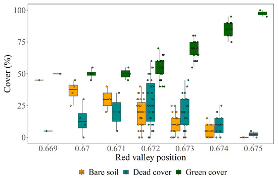
Figure 6.
The influence of dead materials, green vegetation and bare soil on the red valley position based on the simulated hyper-spectra (i.e., only the spectra with clear red absorption characteristics were included in the analysis).
4.2. The Impact of Dead Cover on LAI Estimation
The results of this study indicate that NDVI is superior to the spectral parameters of yellow-edge, red-edge and NIR shoulder for LAI estimation in grasslands. Previous research also shows that vegetation indices calculated using NIR and red band reflectance are more functional than red-edge parameters in grasslands [52]. In mixed grasslands, dead materials or bare soil would cause a slight shift in the red valley position, moving it away from 670 nm (i.e., the common red valley position used in hyperspectral NDVI; Equation (1)). It would enhance the accuracy of NDVI-based LAI estimation to use the accurate reflectance of red valley (Table 4). In addition, NDVI using red valley reduces the effects of dead materials which is superior to the hyperspectral NDVI using the reflectance in 670 nm (Table 3).
We identified two error sources for LAI estimation using NDVI or spectral parameters of yellow-edge, red-edge and NIR shoulder. One was the impact of dead material on in situ measurement of LAI, and a second was the influence of dead material on spectral parameters and NDVI. Plant canopy measuring devices (e.g., Li-cor LAI-2000 and Li-cor LAI-2200 plant canopy analyzer), capturing solar radiation intercepted by the vegetation canopy, are the most popular field method for LAI measurement [53,54,55]. However, research has found that dead materials (i.e., standing dead materials without litter) also contributes to LAI measured by the plant canopy devices, albeit with a smaller contribution than green vegetation [25,56]. Dead material also contributes to NDVI and spectral parameters (e.g., simulated NDVI using red valley is 0.8, 0.16 and 0.13 for 100% green cover, 100% dead cover and 100% bare soil cover, respectively; Figure 5d). Therefore, the linear regression model for LAI estimation becomes less accurate after dead cover exceeds a certain threshold (Table 4). The data range of dead cover is critical for LAI estimation based on the outcomes of our LAI estimation models using NDVI or the spectral parameters of red-edge, yellow-edge and NIR shoulder.
5. Conclusions
Our findings highlight six novel phenomena of spectral grassland measurement: (1) Dead cover has a fan shape relationship with the red-edge slope, the yellow-edge slope, the NIR shoulder slope and NDVI relative to bare soil cover; (2) without considering bare soil cover, dead cover has a positive linear relationship with the yellow-edge slope, a negative linear relationship with the red-edge slope, the NIR shoulder slope and NDVI; (3) the spectral signal of red valley disappears when dead cover exceeds 67%, indicating the spectral characteristics of green vegetation in the wavelength region of yellow-edge is no longer distinct when dead cover is high; (4) large amounts of dead material cause red-edge position shifts to shorter wavelengths (i.e., a blue shift); (5) hyperspectral NDVI, NDVI using the red valley, the yellow-edge slope, the red-edge slope, and red-edge position are all significant spectral indices for LAI estimation, but the estimation accuracy decrease significant when dead cover exceeds 72.3–74.5%; (6) accurate extraction of the red valley position reduces the impact of dead materials and enhances the accuracy of LAI estimation when using hyperspectral NDVI.
Supplementary Materials
The following supporting information can be downloaded at: https://www.mdpi.com/article/10.3390/rs14133031/s1, the script written in R for extracting the spectral parameters in the wavelength region of yellow-edge, red-edge and NIR shoulder automatically from the hyper-spectra.
Author Contributions
Conceptualization, D.X. and W.X.; methodology, D.X.; validation, D.X. and Y.L.; formal analysis, D.X. and Y.L.; investigation, D.X., Y.L. and X.G.; writing—original draft preparation, D.X.; writing—review and editing, D.X., W.X. and X.G.; supervision, W.X.; funding acquisition, W.X. and D.X. All authors have read and agreed to the published version of the manuscript.
Funding
This research was funded by the National Natural Science Foundation of China (41971328), the Science and Technology Program Project Funds of Sichuan Province (2022YFS0490) and the Six Talent Peaks Program of Jiangsu Province (TD-XYDXX-006).
Data Availability Statement
The data presented in this study are available on request from the corresponding author. The data are not publicly available due to the privacy of national parks.
Acknowledgments
The authors would like to acknowledge Wuyishan National Park and Grasslands National Park for the logistical support, and all the field crew for the field data collection. We also acknowledge John Wilmshurst for editing and polishing the English for this manuscript.
Conflicts of Interest
The authors declare no conflict of interest.
Appendix A
Analysis of data collected in GNP only (including the field data collected in situ and transects) based on methods developed in this study.
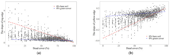
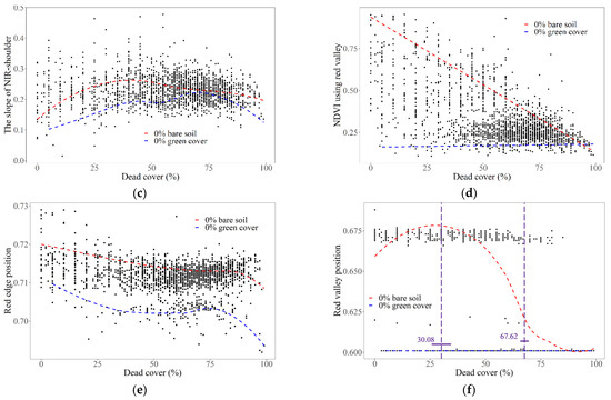
Figure A1.
The relationship between dead cover and the spectral parameters. The relation between dead cover and the slope of red-edge (a), yellow-edge (b), NIR shoulder (c), NDVI using red valley (d), red-edge position (e) and red valley position (f) extracted from field measured hyper-spectra.
Figure A1.
The relationship between dead cover and the spectral parameters. The relation between dead cover and the slope of red-edge (a), yellow-edge (b), NIR shoulder (c), NDVI using red valley (d), red-edge position (e) and red valley position (f) extracted from field measured hyper-spectra.

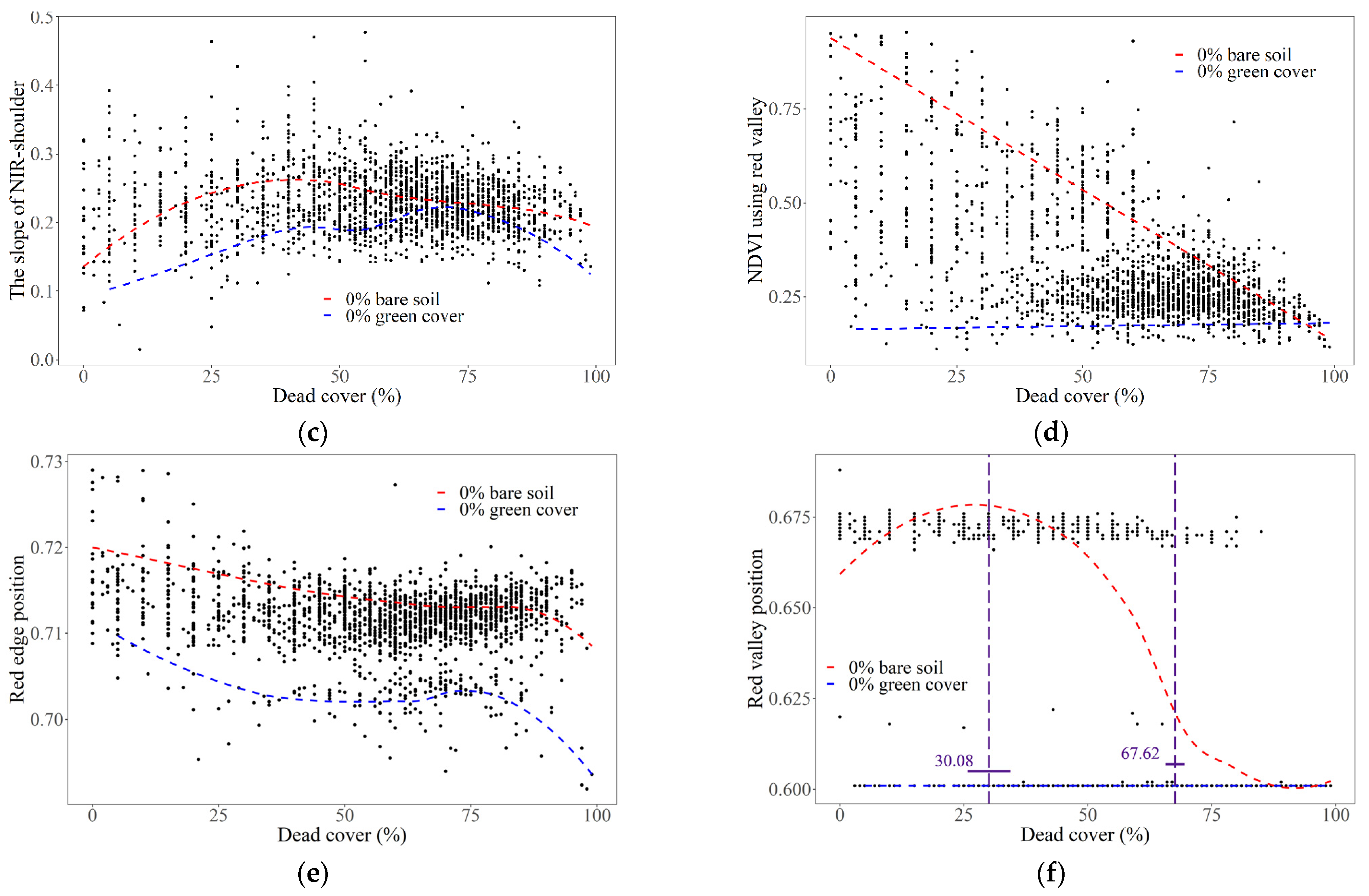
Table A1.
Correlation matrix between LAI and different spectral metrics.
Table A1.
Correlation matrix between LAI and different spectral metrics.
| The Slope of Yellow-Edge | The Slope of Red-Edge | The Slope of NIR Shoulder | Hyperspectral NDVI | NDVI Using Red Valley | LAI | Red-Edge Position | |
|---|---|---|---|---|---|---|---|
| The slope of yellow-edge | −0.94 * | −0.60 * | −0.94 * | −0.94 * | −0.71 * | −0.53 * | |
| The slope of red-edge | 0.70 * | 0.95 * | 0.95 * | 0.76 * | 0.63 * | ||
| The slope of NIR shoulder | 0.65 * | 0.65 * | 0.45 * | 0.41 * | |||
| Hyperspectral NDVI | 1 * | 0.78 * | 0.68 * | ||||
| NDVI using red valley | 0.79 * | 0.69 * | |||||
| LAI | 0.63 * | ||||||
| Red-edge position |
* p < 0.001.
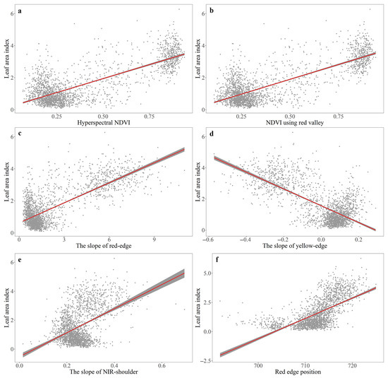
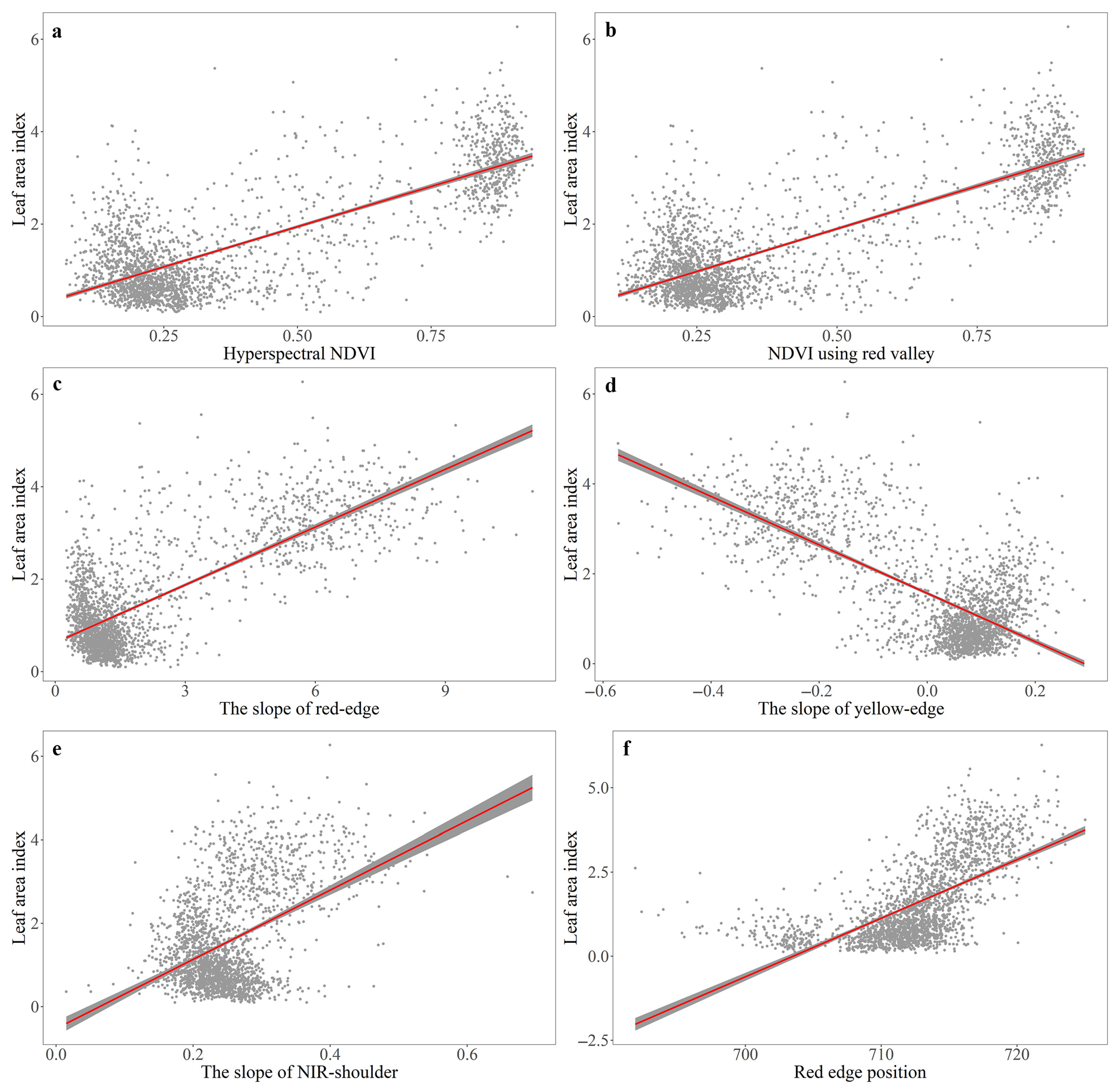
Figure A2.
Linear regression models for LAI (leaf area index) estimation. The relation between LAI and hyperspectral NDVI (a), NDVI using red valley (b), the slope of red-edge (c), yellow-edge (d), the slope of NIR shoulder (e) and red-edge position (f).
Figure A2.
Linear regression models for LAI (leaf area index) estimation. The relation between LAI and hyperspectral NDVI (a), NDVI using red valley (b), the slope of red-edge (c), yellow-edge (d), the slope of NIR shoulder (e) and red-edge position (f).
References
- Xu, D.D.; Guo, X.L.; Li, Z.Q.; Yang, X.H.; Yin, H. Measuring the dead component of mixed grassland with Landsat imagery. Remote Sens. Environ. 2014, 142, 33–43. [Google Scholar] [CrossRef]
- Novara, A.; Ruehl, J.; La Mantia, T.; Gristina, L.; La Bella, S.; Tuttolomondo, T. Litter contribution to soil organic carbon in the processes of agriculture abandon. Solid Earth 2015, 6, 425–432. [Google Scholar] [CrossRef] [Green Version]
- Eckstein, R.L.; Donath, T.W. Interactions between litter and water availability affect seedling emergence in four familial pairs of floodplain species. J. Ecol. 2005, 93, 807–816. [Google Scholar] [CrossRef]
- Guerschman, J.P.; Hill, M.J.; Renzullo, L.J.; Barrett, D.J.; Marks, A.S.; Botha, E.J. Estimating fractional cover of photosynthetic vegetation, non-photosynthetic vegetation and bare soil in the Australian tropical savanna region upscaling the EO-1 Hyperion and MODIS sensors. Remote Sens. Environ. 2009, 113, 928–945. [Google Scholar] [CrossRef]
- Patrick, L.B.; Fraser, L.H.; Kershner, M.W. Large-scale manipulation of plant litter and fertilizer in a managed successional temperate grassland. Plant Ecol. 2008, 197, 183–195. [Google Scholar] [CrossRef]
- Deutsch, E.S.; Bork, E.W.; Willms, W.D. Separation of grassland litter and ecosite influences on seasonal soil moisture and plant growth dynamics. Plant Ecol. 2010, 209, 135–145. [Google Scholar] [CrossRef]
- Bonanomi, G.; Caporaso, S.; Allegrezza, M. Effects of nitrogen enrichment, plant litter removal and cutting on a species-rich Mediterranean calcareous grassland. Plant Biosyst. 2009, 143, 443–455. [Google Scholar] [CrossRef]
- Chen, J.; Yi, S.; Qin, Y.; Wang, X. Improving estimates of fractional vegetation cover based on UAV in alpine grassland on the Qinghai-Tibetan Plateau. Int. J. Remote Sens. 2016, 37, 1922–1936. [Google Scholar] [CrossRef]
- Ge, J.; Meng, B.; Liang, T.; Feng, Q.; Gao, J.; Yang, S.; Huang, X.; Xie, H. Modeling alpine grassland cover based on MODIS data and support vector machine regression in the headwater region of the Huanghe River, China. Remote Sens. Environ. 2018, 218, 162–173. [Google Scholar] [CrossRef]
- He, Y.; Yang, J.; Guo, X. Green Vegetation Cover Dynamics in a Heterogeneous Grassland: Spectral Unmixing of Landsat Time Series from 1999 to 2014. Remote Sens. 2020, 12, 3826. [Google Scholar] [CrossRef]
- Jin, Y.; Yang, X.; Qiu, J.; Li, J.; Gao, T.; Wu, Q.; Zhao, F.; Ma, H.; Yu, H.; Xu, B. Remote Sensing-Based Biomass Estimation and Its Spatio-Temporal Variations in Temperate Grassland, Northern China. Remote Sens. 2014, 6, 1496–1513. [Google Scholar] [CrossRef] [Green Version]
- Meng, B.; Ge, J.; Liang, T.; Yang, S.; Gao, J.; Feng, Q.; Cui, X.; Huang, X.; Xie, H. Evaluation of Remote Sensing Inversion Error for the Above-Ground Biomass of Alpine Meadow Grassland Based on Multi-Source Satellite Data. Remote Sens. 2017, 9, 372. [Google Scholar] [CrossRef] [Green Version]
- Sakowska, K.; MacArthur, A.; Gianelle, D.; Dalponte, M.; Alberti, G.; Gioli, B.; Miglietta, F.; Pitacco, A.; Meggio, F.; Fava, F.; et al. Assessing Across-Scale Optical Diversity and Productivity Relationships in Grasslands of the Italian Alps. Remote Sens. 2019, 11, 614. [Google Scholar] [CrossRef] [Green Version]
- Shang, E.; Xu, E.; Zhang, H.; Liu, F. Analysis of Spatiotemporal Dynamics of the Chinese Vegetation Net Primary Productivity from the 1960s to the 2000s. Remote Sens. 2018, 10, 860. [Google Scholar] [CrossRef] [Green Version]
- Wang, G.; Liu, S.; Liu, T.; Fu, Z.; Yu, J.; Xue, B. Modelling above-ground biomass based on vegetation indexes: A modified approach for biomass estimation in semi-arid grasslands. Int. J. Remote Sens. 2019, 40, 3835–3854. [Google Scholar] [CrossRef]
- You, Y.; Wang, S.; Ma, Y.; Wang, X.; Liu, W. Improved Modeling of Gross Primary Productivity of Alpine Grasslands on the Tibetan Plateau Using the Biome-BGC Model. Remote Sens. 2019, 11, 1287. [Google Scholar] [CrossRef] [Green Version]
- Zhai, D.; Gao, X.; Li, B.; Yuan, Y.; Jiang, Y.; Liu, Y.; Li, Y.; Li, R.; Liu, W.; Xu, J. Driving Climatic Factors at Critical Plant Developmental Stages for Qinghai-Tibet Plateau Alpine Grassland Productivity. Remote Sens. 2022, 14, 1564. [Google Scholar] [CrossRef]
- Hoeppner, J.M.; Skidmore, A.K.; Darvishzadeh, R.; Heurich, M.; Chang, H.C.; Gara, T.W. Mapping Canopy Chlorophyll Content in a Temperate Forest Using Airborne Hyperspectral Data. Remote Sens. 2020, 12, 3573. [Google Scholar] [CrossRef]
- Zhang, A.W.; Hu, S.X.; Zhang, X.Z.; Zhang, T.P.; Li, M.N.; Tao, H.Y.; Hou, Y. A Handheld Grassland Vegetation Monitoring System Based on Multispectral Imaging. Agriculture 2021, 11, 1262. [Google Scholar] [CrossRef]
- Imran, H.A.; Gianelle, D.; Rocchini, D.; Dalponte, M.; Martin, M.P.; Sakowska, K.; Wohlfahrt, G.; Vescovo, L. VIS-NIR, Red-Edge and NIR-Shoulder Based Normalized Vegetation Indices Response to Co-Varying Leaf and Canopy Structural Traits in Heterogeneous Grasslands. Remote Sens. 2020, 12, 2254. [Google Scholar] [CrossRef]
- Polley, H.W.; Yang, C.H.; Wilsey, B.J.; Fay, P.A. Spectrally derived values of community leaf dry matter content link shifts in grassland composition with change in biomass production. Remote Sens. Ecol. Conserv. 2020, 6, 344–353. [Google Scholar] [CrossRef]
- Blackburn, R.C.; Barber, N.A.; Farrell, A.K.; Buscaglia, R.; Jones, H.P. Monitoring ecological characteristics of a tallgrass prairie using an unmanned aerial vehicle. Restor. Ecol. 2021, 29, e13339. [Google Scholar] [CrossRef]
- Wei, H.D.; Yang, X.M.; Zhang, B.; Ding, F.; Zhang, W.X.; Liu, S.Z.; Chen, F. Hyper-spectral characteristics of rolled-leaf desert vegetation in the Hexi Corridor, China. J. Arid Land 2019, 11, 332–344. [Google Scholar] [CrossRef] [Green Version]
- Zhang, T.; Jiang, X.D.; Jiang, L.L.; Li, X.R.; Yang, S.B.; Li, Y.X. Hyperspectral Reflectance Characteristics of Rice Canopies under Changes in Diffuse Radiation Fraction. Remote Sens. 2022, 14, 285. [Google Scholar] [CrossRef]
- Xu, D.D.; An, D.S.; Guo, X.L. The Impact of Non-Photosynthetic Vegetation on LAI Estimation by NDVI in Mixed Grassland. Remote Sens. 2020, 12, 1979. [Google Scholar] [CrossRef]
- Jiang, S.; Wang, F.; Shen, L.M.; Liao, G.P. Local detrended fluctuation analysis for spectral red-edge parameters extraction. Nonlinear Dyn. 2018, 93, 995–1008. [Google Scholar] [CrossRef]
- Liu, C.; Hu, Z.H.; Kong, R.; Yu, L.F.; Wang, Y.Y.; Chen, S.T.; Zhang, X.S. Hyperspectral characteristics and leaf area index monitoring of rice (Oryza sativa L.) under carbon dioxide concentration enrichment. Spectrosc. Lett. 2021, 54, 231–243. [Google Scholar] [CrossRef]
- Kang, Y.; Meng, Q.; Liu, M.; Zou, Y.; Wang, X. Crop Classification Based on Red Edge Features Analysis of GF-6 WFV Data. Sensors 2021, 21, 4328. [Google Scholar] [CrossRef]
- Lin, Y.H.; Shen, H.F.; Tian, Q.J.; Gu, X.F. Improving leaf area index retrieval using spectral characteristic parameters and data splitting. Int. J. Remote Sens. 2020, 41, 1741–1759. [Google Scholar] [CrossRef]
- Sun, Q.; Gu, X.H.; Sun, L.; Yang, G.J.; Zhou, L.F.; Guo, W. Dynamic change in rice leaf area index and spectral response under flooding stress. Paddy Water Environ. 2020, 18, 223–233. [Google Scholar] [CrossRef]
- Gao, J.L.; Liang, T.G.; Yin, J.P.; Ge, J.; Feng, Q.S.; Wu, C.X.; Hou, M.J.; Liu, J.; Xie, H.J. Estimation of Alpine Grassland Forage Nitrogen Coupled with Hyperspectral Characteristics during Different Growth Periods on the Tibetan Plateau. Remote Sens. 2019, 11, 2085. [Google Scholar] [CrossRef] [Green Version]
- Zheng, J.J.; Li, F.; Du, X. Using Red Edge Position Shift to Monitor Grassland Grazing Intensity in Inner Mongolia. J. Indian Soc. Remote Sens. 2018, 46, 81–88. [Google Scholar] [CrossRef]
- Yang, F.F.; Liu, S.P.; Wang, Q.Y.; Liu, T.; Li, S.J. Assessing Waterlogging Stress Level of Winter Wheat from Hyperspectral Imagery Based on Harmonic Analysis. Remote Sens. 2022, 14, 122. [Google Scholar] [CrossRef]
- Klein, D.; Menz, G. Monitoring of seasonal vegetation response to rainfall variation and land use in East Africa using ENVISAT MERIS data. In Proceedings of the 25th IEEE International Geoscience and Remote Sensing Symposium (IGARSS 2005), Seoul, Korea, 25–29 July 2005; IEEE: Piscataway, NJ, USA, 2005; pp. 2884–2887. [Google Scholar]
- Sibanda, M.; Mutanga, O.; Rouget, M. Testing the capabilities of the new WorldView-3 space-borne sensor’s red-edge spectral band in discriminating and mapping complex grassland management treatments. Int. J. Remote Sens. 2017, 38, 1–22. [Google Scholar] [CrossRef]
- Zhu, Y.H.; Liu, K.; Liu, L.; Myint, S.W.; Wang, S.G.; Liu, H.X.; He, Z. Exploring the Potential of WorldView-2 Red-Edge Band-Based Vegetation Indices for Estimation of Mangrove Leaf Area Index with Machine Learning Algorithms. Remote Sens. 2017, 9, 1060. [Google Scholar] [CrossRef] [Green Version]
- Schuster, C.; Foerster, M.; Kleinschmit, B. Testing the red edge channel for improving land-use classifications based on high-resolution multi-spectral satellite data. Int. J. Remote Sens. 2012, 33, 5583–5599. [Google Scholar] [CrossRef]
- Kim, H.-O.; Yeom, J.-M. Effect of red-edge and texture features for object-based paddy rice crop classification using RapidEye multi-spectral satellite image data. Int. J. Remote Sens. 2014, 35, 7046–7068. [Google Scholar] [CrossRef]
- Gholizadeh, A.; Misurec, J.; Kopackova, V.; Mielke, C.; Rogass, C. Assessment of Red-Edge Position Extraction Techniques: A Case Study for Norway Spruce Forests Using HyMap and Simulated Sentinel-2 Data. Forests 2016, 7, 226. [Google Scholar] [CrossRef] [Green Version]
- Guo, X.L.; Wilmshurst, J.F.; Li, Z.Q. Comparison of Laboratory and Field Remote Sensing Methods to Measure Forage Quality. Int. J. Environ. Res. Public Health 2010, 7, 3513–3530. [Google Scholar] [CrossRef]
- Guo, X.; Wilmshurst, J.; McCanny, S.; Fargey, P.; Richard, P. Measuring Spatial and Vertical Heterogeneity of Grasslands Using Remote Sensing Techniques. J. Environ. Inform. 2004, 3, 24–32. [Google Scholar] [CrossRef] [Green Version]
- Xu, D.D.; Geng, Q.H.; Jin, C.S.; Xu, Z.K.; Xu, X. Tree Line Identification and Dynamics under Climate Change in Wuyishan National Park Based on Landsat Images. Remote Sens. 2020, 12, 2890. [Google Scholar] [CrossRef]
- Li, M.; Zheng, Y.; Fan, R.R.; Zhong, Q.L.; Cheng, D.L. Scaling relationships of twig biomass allocation in Pinus hwangshanensis along an altitudinal gradient. PLoS ONE 2017, 12, e0178344. [Google Scholar] [CrossRef] [PubMed]
- Lin, F.F.; Guo, S.; Tan, C.W.; Zhou, X.G.; Zhang, D.Y. Identification of Rice Sheath Blight through Spectral Responses Using Hyperspectral Images. Sensors 2020, 20, 6243. [Google Scholar] [CrossRef] [PubMed]
- Li, D.; Tian, L.; Wan, Z.F.; Jia, M.; Yao, X.; Tian, Y.C.; Zhu, Y.; Cao, W.X.; Cheng, T. Assessment of unified models for estimating leaf chlorophyll content across directional-hemispherical reflectance and bidirectional reflectance spectra. Remote Sens. Environ. 2019, 231, 111240. [Google Scholar] [CrossRef]
- Wu, C.; Niu, Z.; Tang, Q.; Huang, W. Estimating chlorophyll content from hyperspectral vegetation indices: Modeling and validation. Agric. Forest Meteorol. 2008, 148, 1230–1241. [Google Scholar] [CrossRef]
- Asner, G.P.; Lobell, D.B. A biogeophysical approach for automated SWIR unmixing of soils and vegetation. Remote Sens. Environ. 2000, 74, 99–112. [Google Scholar] [CrossRef]
- Ustin, S.L.; Valko, P.G.; Kefauver, S.C.; Santos, M.J.; Zimpfer, J.F.; Smith, S.D. Remote sensing of biological soil crust under simulated climate change manipulations in the Mojave Desert. Remote Sens. Environ. 2009, 113, 317–328. [Google Scholar] [CrossRef]
- Duan, M.J.; Gao, Q.Z.; Wan, Y.F.; Li, Y.; Guo, Y.Q.; Ganzhu, Z.B.; Liu, Y.T.; Qin, X.B. Biomass estimation of alpine grasslands under different grazing intensities using spectral vegetation indices. Can. J. Remote Sens. 2011, 37, 413–421. [Google Scholar] [CrossRef]
- Jiang, C.; Chen, Y.; Wu, H.; Li, W.; Zhou, H.; Bo, Y.; Shao, H.; Song, S.; Puttonen, E.; Hyyppae, J. Study of a High Spectral Resolution Hyperspectral LiDAR in Vegetation Red Edge Parameters Extraction. Remote Sens. 2019, 11, 2007. [Google Scholar] [CrossRef] [Green Version]
- Chen, J.; Gu, S.; Shen, M.G.; Tang, Y.H.; Matsushita, B. Estimating aboveground biomass of grassland having a high canopy cover: An exploratory analysis of in situ hyperspectral data. Int. J. Remote Sens. 2009, 30, 6497–6517. [Google Scholar] [CrossRef]
- Liu, Z.-Y.; Huang, J.-F.; Wu, X.-H.; Dong, Y.-P. Comparison of vegetation indices and red-edge parameters for estimating grassland cover from canopy reflectance data. J. Integr. Plant Biol. 2007, 49, 299–306. [Google Scholar] [CrossRef]
- Liu, X.H.; Wang, L. Feasibility of using consumer-grade unmanned aerial vehicles to estimate leaf area index in Mangrove forest. Remote Sens. Lett. 2018, 9, 1040–1049. [Google Scholar] [CrossRef]
- Zhang, J.; Yang, C.H.; Zhao, B.Q.; Song, H.B.; Hoffmann, W.C.; Shi, Y.Y.; Zhang, D.Y.; Zhang, G.Z. Crop Classification and LAI Estimation Using Original and Resolution-Reduced Images from Two Consumer-Grade Cameras. Remote Sens. 2017, 9, 1054. [Google Scholar] [CrossRef] [Green Version]
- Lin, Q.A.; Huang, H.G.; Yu, L.F.; Wang, J.X. Detection of Shoot Beetle Stress on Yunnan Pine Forest Using a Coupled LIBERTY2-INFORM Simulation. Remote Sens. 2018, 10, 1133. [Google Scholar] [CrossRef] [Green Version]
- Li, Z.Q.; Guo, X.L. A suitable vegetation index for quantifying temporal variation of leaf area index (LAI) in semiarid mixed grassland. Can. J. Remote Sens. 2010, 36, 709–721. [Google Scholar] [CrossRef]


Publisher’s Note: MDPI stays neutral with regard to jurisdictional claims in published maps and institutional affiliations. |
© 2022 by the authors. Licensee MDPI, Basel, Switzerland. This article is an open access article distributed under the terms and conditions of the Creative Commons Attribution (CC BY) license (https://creativecommons.org/licenses/by/4.0/).