Abstract
The star tracker is a prerequisite device to realize high-precision attitude determination for a spacecraft. However, due to the errors in optical lens machining, optical path assembly, and temperature alternation, optical instruments suffer from some amount of optical geometric distortion, resulting in declining star tracker accuracy. The on-orbit distortion correction of star images is indispensable for precise performance. In this paper, a novel single-layer 2D Legendre neural network (2DLNN) to automatically correct the geometric distortion of the star tracker is proposed. An offline training method grounded on batch star images and an online training algorithm based on sequential star images are designed, respectively. The 2DLNN realizes the ground-based and on-orbit online correction of optical geometric distortion for the star tracker. The 2DLNN features self-learning, lifelong learning, and good adaptability. The single-layer neural network is simple, quick convergence, which is suitable for on-orbit implementation. The simulations demonstrate that the average distortion error can be reduced to less than 0.04 px after ground-based training. In the earth-orientation mode of the LEO satellite, the on-orbit sequential training algorithm can converge in 2500 star images under 1 frame/s. The proposed 2DLNN can achieve high-precision correction at the sub-pixel level, effectively improving the star tracker’s attitude determination accuracy.
1. Introduction
Star trackers are the most accurate attitude measurement instruments for spacecraft. They are widely applied in multiple fields and missions, such as self-contained navigation, environmental monitoring, global communication, national security, and deep-space exploration [1,2,3,4,5]. In recent years, with the release and implementation of satellite constellations [6,7], the developing trend of star trackers is miniaturization and low cost. However, the requirements for star trackers are surging rather than falling, which brings greater challenges to star trackers.
Regardless of the the craftsmanship of the optical system of the star tracker, all-optical instruments, whether ground-based or space-based, suffer from some amount of optical geometric distortion. Optical lenses with a large field of view (FOV) will generate a large amount of nonlinear distortion, and the distortion can reach more than two pixels at the image plane edge. These distortions have multiple origins that induce different behavior. They may be static, resulting from unavoidable errors in the shape and placement of the optics or from the imperfect fabrication of the detectors. In general, laboratory calibration and testing are conducted to obtain true values of all parameters, and these errors contribute little to the distortion of the star images [8,9,10,11,12,13].
Distortion may be dynamic; many factors, such as intense vibration during launching, component aging, temperature effects [14,15,16] and a variable environment during operation, alter the systematic errors and change the camera parameters on orbit [17,18], resulting in the star spot imaging being uneven in energy distribution and asymmetrical shape. Star trackers use a detector with a rolling shutter, usually active pixel sensors (APS). Under dynamic conditions, it is well-known that the detected star image is deformed. The centroid of the starspot is shifted [19,20,21]. Consequently, the accuracy of extracting the centroid is directly impacted. To guarantee and ensure the attitude accuracy and the safety of the spacecraft, it is essential to establish and optimize the distorted models to complete the correction of distorted star images.
The on-orbit calibration or distortion correction for spacecraft attitude star trackers was first proposed by Samaan [22], in which the method makes use of residuals between measured inter star cosine angles and the inter star cosine angles between the corresponding cataloged stars to learn the calibration corrections on orbit. The approach makes use of the truth that inter star angles are an invariant of rotational transformations. Therefore the correction process is naturally divided into two major parts, calibration of the principal point offset and focal length and then calibration of the focal plane distortions.
Based on Samaan’s method, various on-orbit calibration algorithms have been developed. The attitude-dependent methods [23,24,25,26], gyroscopes, infrared horizon sensors, sun sensors and other attitude devices are required to determine the initial attitude information first. However, the error of the star tracker frame attitude affects the correction inevitably. Thus, the attitude-independent approach has been proposed. Many attitude-independent algorithms estimate the star tracker optical parameters by directly utilizing the star coordinate in the star image plane and the corresponding star vector in the inertial coordinate frame. The most commonly used of these methods are the least-squares method and the Kalman Filter algorithm [17,18,22,23,27,28,29,30,31,32,33].
In these methods, the simple second-order radial distortion model is considered. To correct the starspot position error caused by the rolling shutter exposure, the authors of [20] used a first-order approximation of the real motion of the stars across the detector. The proposed strategy set the centroids to the same time instant. In Ref [21], the authors corrected the starspot position at an asynchronous time to the same time based on time-domain constraints. The focal length errors and the principal point will affect the accuracy of star identification, and the above methods are based on the assumption that the principal point and focal length change greatly. In this paper, the errors caused by the change of principal point are considered systematic errors, and the random error is not considered.
Methods based on polynomial fitting have been developed to correct other complex distortions. Ordinary polynomials fit the mapping relationship between distorted stars and reference stars. Wei [34] used the improved genetic algorithm to obtain the optimal coefficient, while Liu [35] utilized machine learning to solve the polynomial fitting. However, according to the author of the paper [36], it has been proven that the solution of ordinary polynomials is the system of linear equations, known as the normal equations.
As the order or the numbers of polynomials increases, however, solving a large system of equations becomes unstable and inaccurate. Compared with ground-based correction, the biggest problem of on-orbit correction is that the types of distortion are often unknown. Some distortions are stable, such as radial distortion and tangential distortion caused by the change of the optical system parameters. There are also some image distortions caused by other factors, such as perspective distortion.
We aim to design an algorithm that can automatically correct the star coordinates of the on-orbit star tracker and is insensitive to the type of image distortion. In this paper, a novel on-orbit geometric distortion correction method that combines 2D Legendre polynomials and a neural network is proposed. To avoid the problem of instability and inaccuracy, 2D normalized Legendre polynomials that are orthogonal polynomials are used to replace the ordinary polynomials. A 2D Legendre neural network (2DLNN) is constructed to obtain the optimal coefficient of the Legendre polynomial.
The neural network has strong adaptability and fast convergence speed, and can also correct any distorted star images. For the different distortions that may occur in the lifelong period of on-orbit star trackers, we can adaptively learn the distortion model by adjusting the number of neurons. Simulations and experiments are conducted to show effectiveness and superiority. The proposed correction method has the potential to become a universal geometric distortion correction framework for star trackers.
Our main contribution is to propose learning-based methods to correct a wide range of geometric distortions of star trackers blindly. More specifically, we propose:
- A single-layer 2D Legendre neural network, which learns the coefficients of 2D Legendre polynomial.
- An offline training method grounded on the batch star images, which realizes the initial correction of the star tracker.
- An on-orbit online learning algorithm based on the sequential star images, which realizes lifelong autonomous distortion correction of the star tracker.
The paper is organized as follows. In Section 2, measurement models related to the star tracker are described. In Section 3, the architectures of 2DLNN are described. Two training methods of offline and online learning are given in detail. In Section 4, the simulation results are shown, and in Section 5, our conclusions and final remarks are reported.
2. Measurement Model of the Star Tracker
2.1. Ideal Model
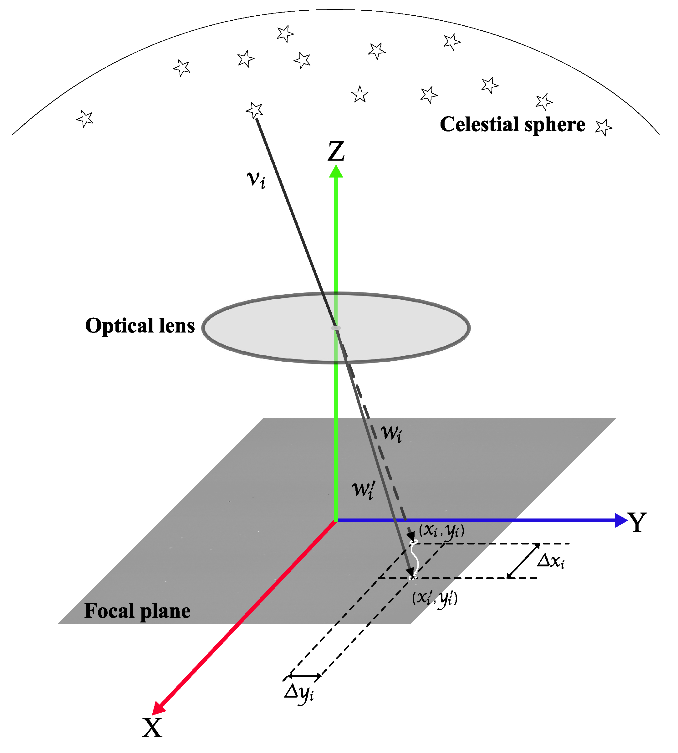
The star tracker is designed to measure the stars’ direction vector. The ideal measurement model of the star tracker can be considered as a pinhole imaging system [1], as shown in Figure 1.
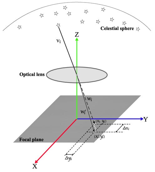
Figure 1.
Pinhole imaging system and real star tracker measurement model. Under the ideal condition, the centroid of stars is in the pinhole imaging system. Due to noise and distortion, there are inevitable errors in the real star tracker measurement model. The real centroid is . The real imaging system is based on the pinhole imaging system.
The i- measurement star vector in imaging frame can be expressed by Equation (1),
where is the i- star centroid, and f is the focal length of the optical system.
The relationship between and can be expressed as follows,
where is the direction vector of the navigation star, and A is the attitude matrix of the star tracker. When the number of navigation stars exceeds two, the attitude matrix can be estimated by the QUEST [37,38] algorithm.
2.2. Typical Star Image Distortion Model
The existence of errors and noise in the optical imaging system is inevitable. Noise in the CMOS APS sensor is a combination of dark current, single point noise, Gaussian readout noise, Poisson noise, fixed pattern noise, etc. [39]. The aberrations in the optical system usually consist of radial distortion [40], tangential distortion [41], thin prism distortion [42] and image transformation [43]. Due to the various influencing factors in space, the optical system parameters may change, and various types of geometric distortion will inevitably occur in star images. Hence, the pinhole model cannot fit with real star imaging exactly.
The relationship between the distorted star spot coordinates and the real star spot coordinates can be expressed by Equation (3),
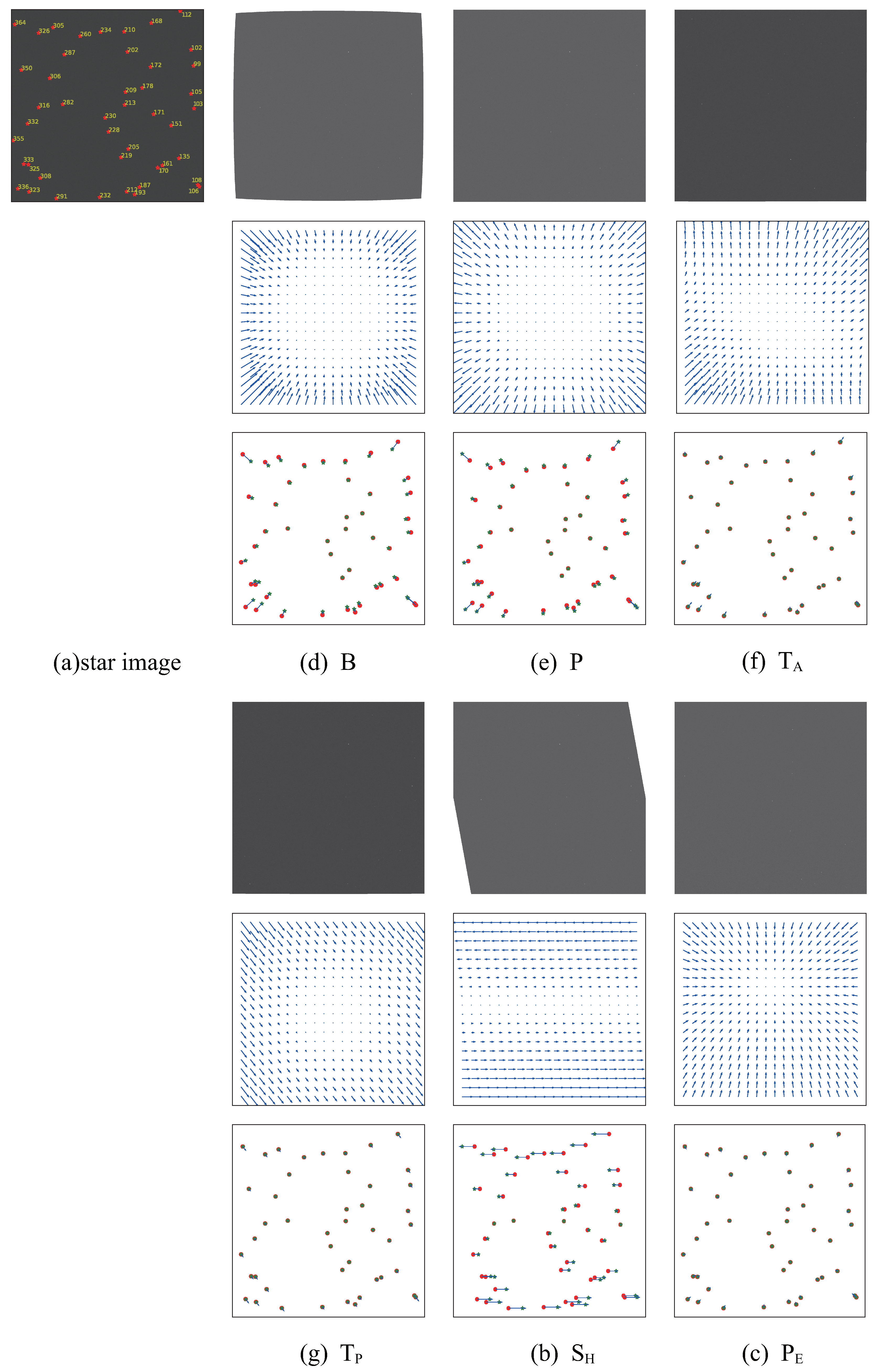
where is the distorted magnitude of star coordinates caused by the change in the parameters of the star tracker. In this paper, five distortions and their causes are briefly described. The manifold distorted star images, the distorted flow of pixels, and the changing of starspot coordinates are shown in Figure 2. Several common distortions of the on-orbit star tracker are shown below.
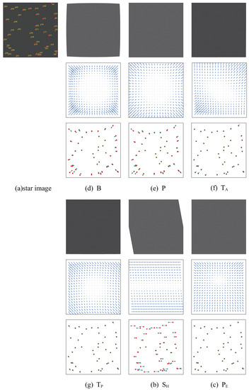
Figure 2.
Various optical distortions models, (a) the star image without distortion and star images with distortion of (b) shear, (c) perspective, (d) barrel, (e) pincushion, (f) tangential and (g) thin prism. The second line is the distortion flow of pixels for various distortion models. The third line is the distortion flow of the starspot position.
- Radial DistortionThe vertical magnification of the optical system in different fields of view is different. The light is more crooked from the center to the edge of the lens, which results in radial distortion and is the main source of distortion. The expression of radial distortion is shown in Equation (4),where n is the order of Taylor expansion, is the distance of the distortion star and the center of the image plane, and is the i- radial distortion coefficient. Barrel distortion typically has a negative term for , whereas pincushion distortion will have a positive value.
- Tangential DistortionThe coaxial error of the optical components in the optical system leads to tangential distortion, and the expression of this type of distortion is shown in Equation (5),where and are the tangential distortion coefficients.
- Thin Prism DistortionThe thin prism distortion is caused by the tilt of the optical component, which is equivalent to inserting a thin prism into a non tilted optical component. The thin prism distortion can be expressed by Equation (6),where and are the thin prism distortion coefficients.
Generally, typical distortions of the star trackers are often a superposition of the three distortions described above. Image transformation is also considered in this paper to test the extendability and adaptability of the proposed method. Different image transformations can be expressed as follows,
- Shear Distortionwhere and are the coefficients of shear distortion.
- Perspective DistortionPerspective distortion can be regarded as an imaging plane transformed into a new imaging plane [8], and the relationship between two imaging planes is transformed by a transformation matrix.where are the elements of the transformation matrix.
2.3. Legendre Polynomial Distorted Modeling
The coordinate of measured star i is noted as , the corresponding reference coordinate of star i is , by using the distortion function as ,
where and are the j- distortion model of X direction and Y direction, respectively.
Here, we can use different functions to describe the distortion of the star images. Most commonly, 2D polynomials up to third or fifth order, depending on the authors, are used as image distortion models. For example, Wei [34] used a third-order polynomial fitting to correct distortion. The improved genetic algorithm was adopted to obtain the optimal solutions. Liu [35] used machine learning to solve the coefficients of ordinary polynomials. However, polynomials are unstable and inaccurate for solving a large system of equations.
To avoid this, orthogonal polynomials should be used. The authors of [44] compared the efficiency of different models: 2D Cartesian polynomials, bivariate B-spline, and 2D Legendre polynomial. They concluded that the 2D Legendre polynomial basis provides faster convergence and lower residuals. Simultaneously, the authors of [45] defined an orthogonal polynomial, which is well adapted to describe the distortion on square images. Finally, the ascending polynomial degree organization of the basis is convenient for characterizing the distortion using a limited number of modes.
Each Legendre polynomial is an n- degree polynomial and may be expressed in one dimension by Equation (11),
As each mode contains the same amount of distortion in both directions (x and y), the polynomials need to be normalized. The final basis of 2D Legendre polynomials can be expressed by Equation (12),
where is the number of modes considered, it determines the dimension of the vector and can be calculated by Equation (13),
where n is the order of the Legendre polynomial, and is the n- degree normalized Legendre polynomial,
Hereafter, the mode of every Legendre polynomial can be expressed by Equation (17),
finally, the coordinates of the i- star in the j- frame, on which a distortion function and can be written as Equation (18),
where and are referred to as the distortion coefficients of the X and Y directions, respectively.
The statistical properties of the noise that we should consider to build the distortion model must be consistent with the noise present in the measurement of star positions. We assume here a noise that follows a Gaussian white noise. The final distortion model is
where is the observation error caused by imaging noise and other factors, which is regarded as the independent Gaussian noise.
3. Legendre Neural Network
The fully-connected neural network implicitly learns the relationship between the camera and the global coordinate system [33], which is proven effective; however, the structure is complicated. Traditional neural networks have drawbacks, such as difficulty determining initial weights and the number of layers and neurons. In general, the convergence time is also long when trained by the backpropagation algorithm.
In the previous section, we defined the direct model. To solve the distortion problem, we now aim to inverse this model by minimizing a criterion. In this paper, a single-layer neural network based on the Legendre polynomial is developed to avoid the problems of traditional neural networks and is named 2DLNN. The single-layer neural network is simple enough to reduce the calculation time to implement the distortion correction algorithm in orbit.
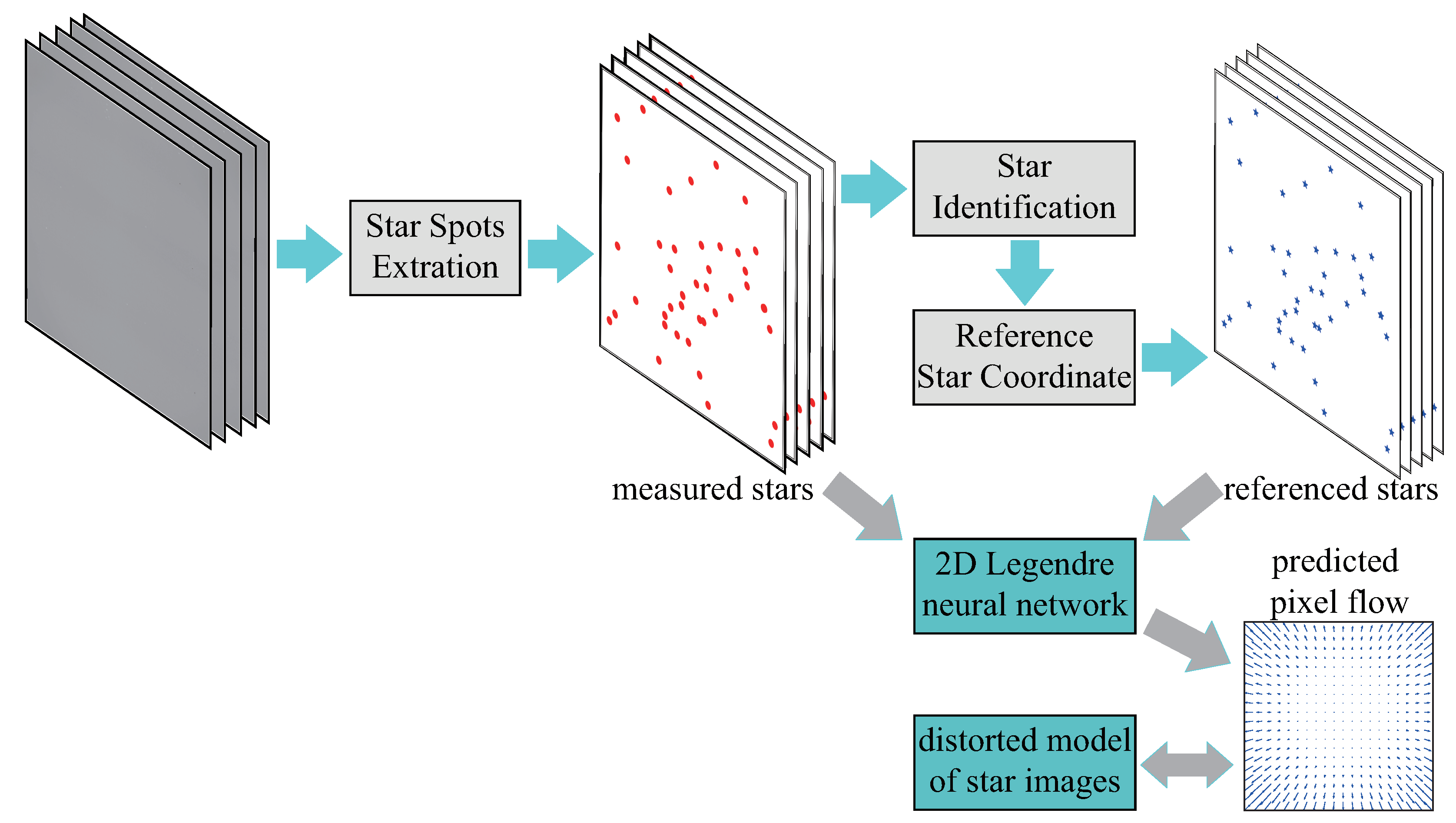
No complicated activation function is included, making it possible to have a rapid response to obtain the results from the input data. The hyper-parameters of the network do not require much tuning. In addition, the authors of [46,47] had proven that a function could be approximated by an orthogonal function set (such as the Legendre function), and the coefficients are unique and bounded. Orthogonal polynomials functions have recursive properties to determine their expansion terms. The flow chart of the geometric distortion correction method based on 2DLNN is shown in Figure 3.

Figure 3.
On-orbit geometric distortion correction procedures.
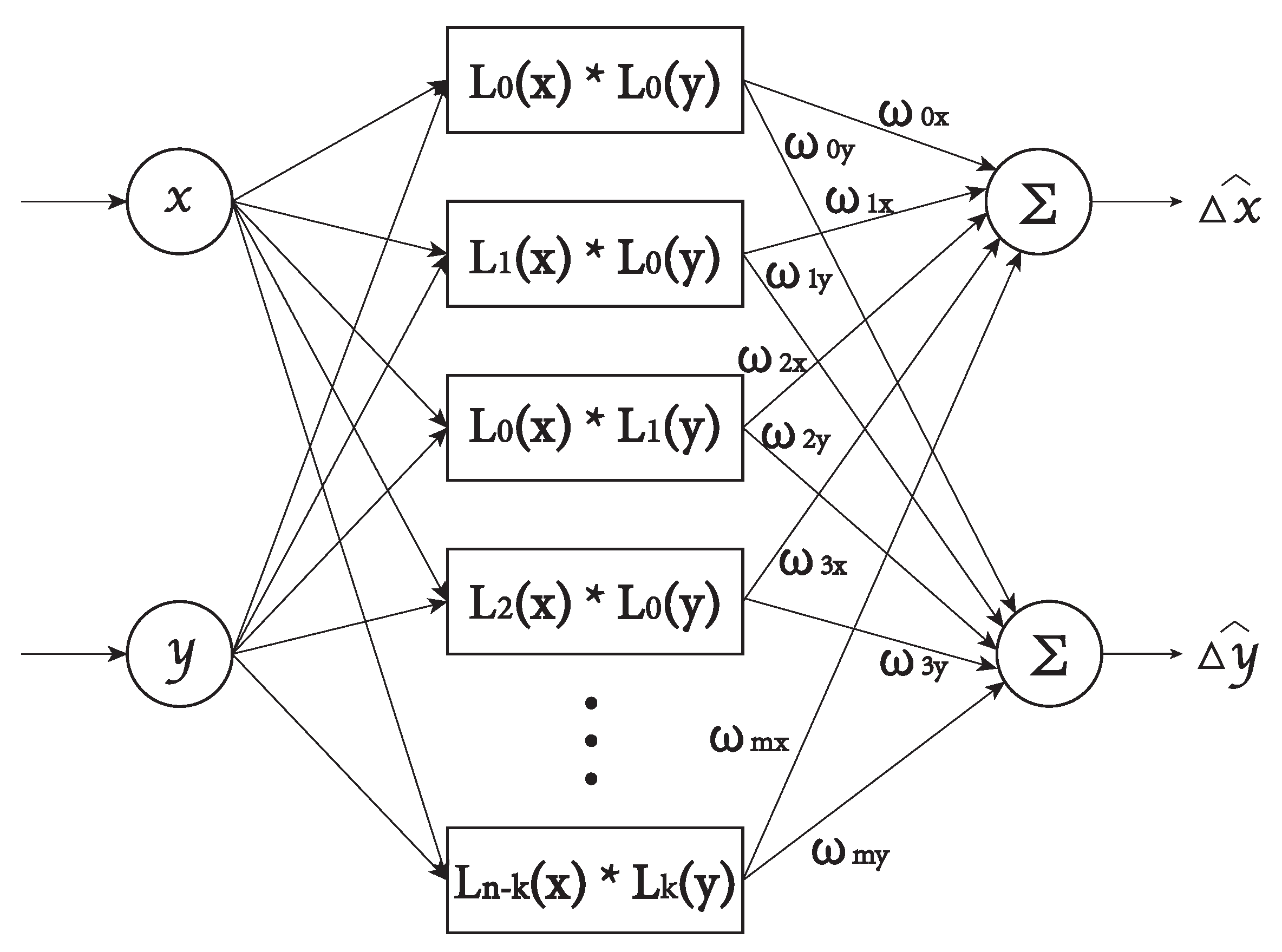
3.1. Network Architectures
In this paper, the optimal coefficients of the Legendre polynomial are solved to fit the distortion of star images. The distortion modeling of the star images can be described as Equation (19), are the parameters that need to be estimated. The input of the 2DLNN is the coordinates of measuring stars, the output is the offset of coordinates between the measured stars centroid and the centroid of reference stars. Consequently, the 2D Legendre neural network is constructed to learn the mapping of measuring stars’ coordinates and coordinates offset. The estimation offset is the 2D vector field that specifies where pixels in the star image with distortion should move to find the corrected coordinates.
According to Equation (19), a single-layer Legendre neural network as shown in Figure 4 can be built.
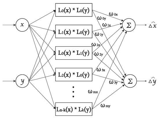
Figure 4.
The structure of the Legendre neural network.
The 2DLNN is trained to minimize the error between the estimated displacement of coordinates and the position offset. The offset is the distance between measuring stars and reference stars. Equation (19) can be abbreviated as Equation (20),
The 2DLNN can be expressed by Equation (21), taking the distortion in the x direction as an example, and the distortion in the y direction can be obtained in the same way.
where is the estimation error of starspot position, is the estimated coefficients of 2D Legendre polynomials.
According to Figure 4, the input of the network is the measuring starspot coordinates , and the output is the coordinate offset . The processing elements are duplicated from the expansion terms of the normalized Legendre polynomials. The n- processing element is identical to the n- expansion term of the 2D normalized Legendre polynomials.
The weights concatenating the mid-layer and the out-layer are needed to update. The single-layer neural network has two sets of adjustable weights which are , and these weights will be trained to approach the desired weights or coefficients in the Equation (19) by the training algorithm. Since each output has unique and independent weights, the two sets of weights can be trained separately.
3.2. Ground-Based Batch Learning
After having built the 2D normalized Legendre neural network, it is necessary to find a method to adjust the weights to approach the desired weights W defined in Equation (20). The training method of 2DLNN in the ground-based calibration is introduced first. The star images can be captured from random areas of the sky, and the distribution of stars is easier to cover the whole field of view of the star tracker, which is conducive to learning the global distortion model of the star image. Therefore, it is a point-to-point training method in the ground-based experiment, which learns the mapping from the whole star image datasets.
The loss is defined as Equation (23),
The gradient descent algorithm is adopted for the weights update. According to the chain rule, the extreme value of can be obtained by calculating the first-order partial differential of , as shown in Equation (24),
The Adam algorithm [48] is adopted to update the weights of 2DLNN. Adam has the attractive benefits of being straightforward to implement with low memory requirements, and the hyper-parameters have intuitive interpretation and typically require little tuning. It is suitable for on-orbit applications. Its convergence has been proven theoretically. Therefore, the weights updating of 2DLNN can be expressed by Equation (25),
where is the forgetting factor, and are the parameters of Adam. is a positive gain, referred to as the learning rate or step size. Equation (25) is the training algorithm used to train the weights. The author of Adam proved that would decrease gradually and reach a stable status. The Adam is described more fully in the Appendix A Equation (A1); however, a brief summary is given here.
3.3. On-Orbit Online Learning
Due to the limitation of satellite storage, the star tracker cannot store a large number of star images and starspot coordinates. It is unrealistic to use the point-to-point training method for the on-orbit star tracker. We first calculate the starspot coverage rate at a specific time for the star tracker orbiting the earth. Then, the online training method is proposed.
3.3.1. Coverage of Star Spot
It is impossible to verify the algorithm directly on orbit, we simulate the state of the star tracker orbiting the earth. To ensure that the proposed method can learn the distortion model of the whole focal plane, stars in a period need to cover most of the star image. The coverage rate of starspot is expressed by a ratio of the area covered by stars in FOV to the area of the entire focal plane in time t, as shown in Equation (26),
where is the area of the contour profile (not convex hull) of all stars within the time interval t, is the area of the focal plane, and the unit of them is .
The star images are photoed along the orbit. The Monte Carlo algorithm is used to calculate the average star coverage rate in the time t, which is shown in Table 1. The sampling time is 1 s, and the orbit is the Starlink (altitude: 550 km, inclination: 53°), and the right ascension and declination of the orbit are generated from the System Tool Kit (STK) software.

Table 1.
Average coverage rate of star spot for different times.
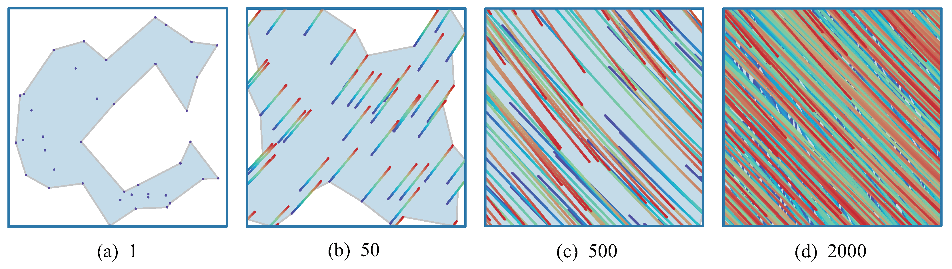
The superposition of starspots in FOV at a different time is shown in Figure 5. They are collected along the Starlink orbit, and the sampling start is determined by the Monte Carlo method. Scatters with the same colors represent stars from the same star image. The coverage area is the envelope of these superimposed stars, as shown in Figure 5a the pale blue background. The coverage rate of stars increases with the increase of star images. Although the coverage rate of 500 frames is high, there are obvious holes in the envelope, and the superposition of 2000 frames covers the entire FOV.
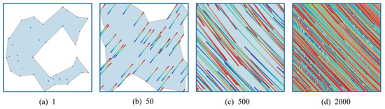
Figure 5.
Stars distribution for different sampling time: (a) the stars distribution in 1 s, where the green background is the profile of the superposed star spots. (b–d) the stars in 50 s, 500 s and 2000 s, respectively.
The stars can be regarded as passing through the FOV of the star tracker at a certain angular velocity. In the engineering application, the probability of starspot being correctly identified increases when the stars are in a position with less distortion, and the correctly identified stars can be tracked in real-time. When the tracked star moves to a position with large distortion, it can continue to be used for distortion correction. In Figure 5, it can be seen that the stars enter the FOV from multiple directions so that 2DLNN can learn and correct the global distortion.
3.3.2. On-Orbit Learning Algorithm
The geometric distortion correction of the on-orbit star tracker is implemented frame-to-frame along the orbit. The loss should be determined by the root mean square error (RMSE) of all correctly identified stars in each frame of the star image. The loss is expressed by Equation (27),
where N is the number of correctly identified stars in a single star image, i represents the centroid coordinates of i- measuring star, and N is different in each star image.
The gradient of online training can be also obtained according to the chain rule, which is expressed by Equation (28),
The optimal coefficient of the 2D Legendre polynomial is obtained by calculating the minimum gradient of the loss.
3.4. Optimum Order of the Legendre Polynomial
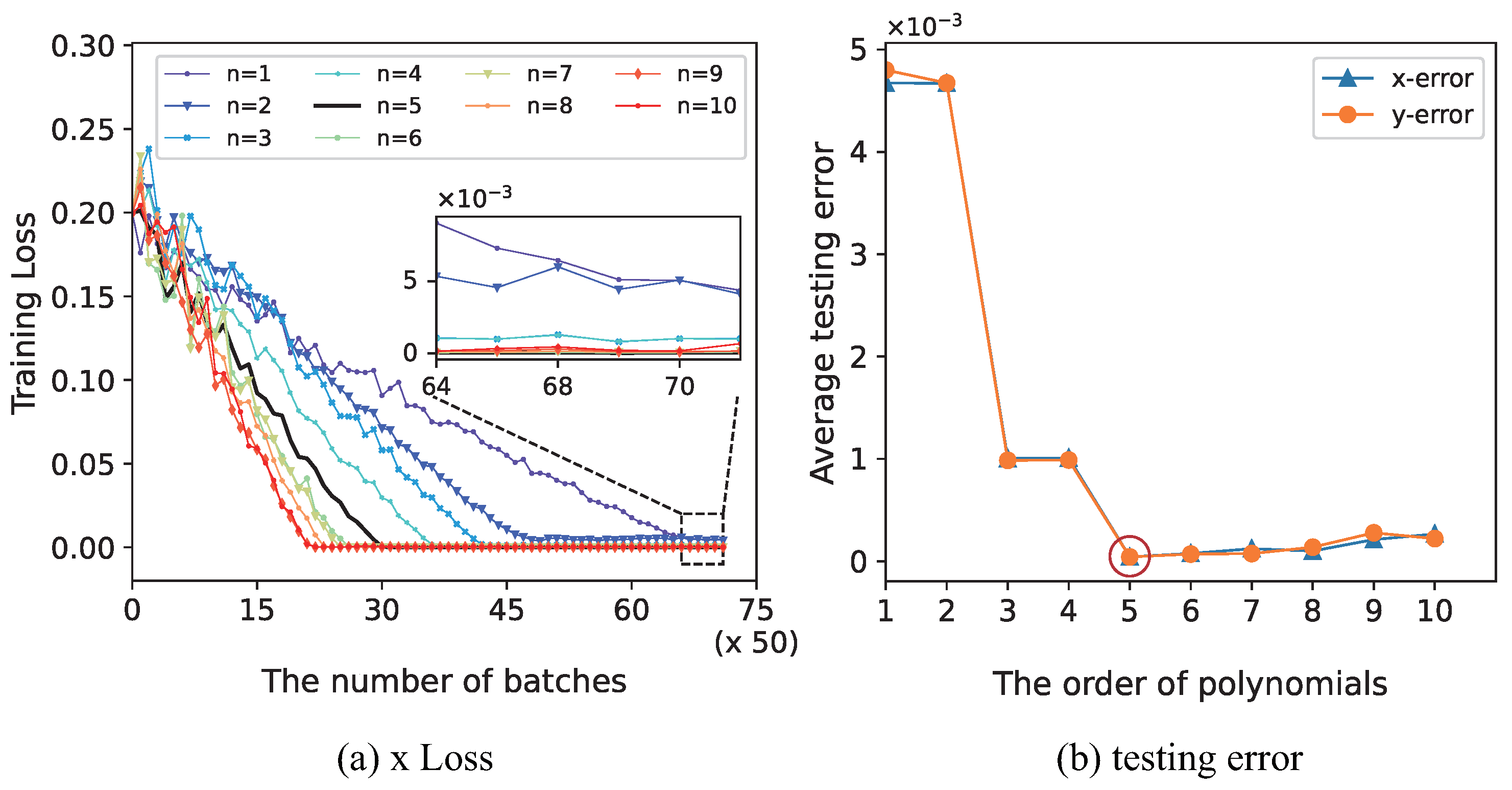
The orders of the Legendre polynomial will have an impact on the results of 2DLNN. The order determines the number of neurons in the neural network, which directly impacts the ability of distortion correction. If the order is too small, the star tracker distortion model cannot completely be expressed by the Legendre polynomials. If there are too many neurons, the network structure is large, and the dataset would not be enough to fit the network. Therefore, it is necessary to find a suitable order for the better ability of 2DLNN.
We analyze the influence of polynomial order on training results. Taking radial distortion as an example, 2DLNN with orders increasing from 1 to 10 are trained, respectively. The corresponding network is applied to the testing dataset. The training results of different orders are shown in Figure 6.
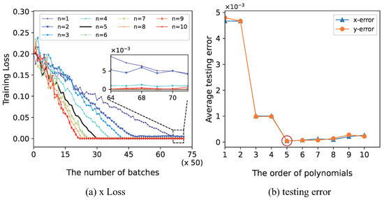
Figure 6.
The training loss and the average testing error for different orders of the 2D Legendre neural network: (a) the training loss at x-axis direction and (b) the average testing error at x-axis and y-axis direction. The optimum order should be the black curve in diagram (a) and the red circle in diagram (b).
Figure 6a is the result of the training dataset, and Figure 6b is the performance of the corresponding network on the testing dataset. When the order is small, the rate of convergence of 2DLNN is slow. The low-order 2DLNN is not convergent on the testing data, indicating that the low-order 2DLNN is underfitting. When the order is 5 or larger, the error remains the minimum on training data (black curve in Figure 6a) and testing data (red circle in Figure 6b). In practical application, the common orders in the optical distortion model are 4 to 6. Considering the time and memory complexity, the optimum order of the 2DLNN should be 5.
3.5. Pseudocode
We summarize our methods for geometric distortion correction of star images in Appendix B Algorithm A1.
4. Experiment and Analysis
Several sets of experiments were designed to verify the validity of the proposed method. They are ground-based and on-orbit experiments. The star images can be captured from random or continuous sky regions in the real night sky observation experiment. The stars in the star images from random sky areas are uniformly distributed, and the numbers are enough for batch learning. The star images obtained from the continuous sky areas were generated along the orbit, which is suitable for frame-to-frame online learning. In the earth-orientation mode of the LEO satellite, the star images generated along the orbit were used to analyze the implementation of the on-orbit training method.
The measurement model was adopted from Figure 1 in Section 2.1. The parameters of the star tracker utilized in the experiments are shown in Table 2. The optical system distortion (radial distortion, tangential distortion and thin prism distortion) and image transformation (shear transformation and perspective transformation) were tested, respectively. The parameters of various distortions are shown in Table 3 and Table 4, the distortion model is adopted in Section 2.2.
Table 2.
Star tracker parameters.
Table 3.
Parameters of optical system distortion.
Table 4.
Parameters of star image transformation.
All experiments and algorithms were simulated in PyCharm CE (V2021.3) with Python 3.8 & Pytorch on a PC with a 2.30 GHz Intel Xeon Gold 6139 CPU of 32 GB RAM, NVIDIA Quadro P4000 GPU of 8 GB RAM and Windows 10 operational system.
4.1. Training Dataset of Star Images
Since real star images are rarely downloaded from on-orbit star trackers, it is unrealistic to use real star images as datasets. In this paper, the star image datasets were collected and generated based on the real on-orbit star tracker parameters. At the same time, the star images datasets were mixed with star images obtained in other ways. The parameters setting of the star tracker in the datasets were the same. The star image datasets are mainly composed as follows.
- Inspired by the literature [18], star images can be captured randomly from Starry Night, a professional and powerful astronomical software, and the digital platform is utilized to obtain the distorted data.
- According to the parameters of the real on-orbit star tracker, the method [49] for generating simulation star images was adopted. Random background noise and random position noise were added to these star images.
- Star images were taken from the real night sky observation experiments, using the star trackers’ parameters in Table 2.
Star images were distorted according to the real distortion model of the star tracker in orbit, which is mainly caused by the change in optical system parameters. The star spot extraction algorithm [39,50,51,52] and the star identification algorithm [53,54,55] were adopted to obtain navigation stars. Then, the transfer matrix from celestial sphere frame to star tracker frame can be calculated using QUEST [37,38] or TRIAS [56] method. The reference starspot coordinates can be obtained through the coordinate transforming equations. The offset distance between the measured starspots and the reference starspots was used as the training label of 2DLNN. Meanwhile, the stars’ centroid coordinates were used as the training data.
The datasets were divided into three parts: ground-based star images from random sky areas (named after GRD) and continuous sky areas (named after GCD). The on-orbit star images along the Starlink orbit (named after OD).
4.2. Simulation of Ground-Based Correction
There is no need to select specific starspots; all available stars in the star images can participate in network model fitting. In the ground-based experiment, we combine the available star coordinates into a complete dataset (namely GRD and GCD). The centroid coordinates of the stars obtained from the distorted star images were used as the input of 2DLNN. Meanwhile, the coordinate offsets were used as the training label. The error will be trained to the minimum. The dataset is randomly divided into training and testing datasets according to the ratio of 8:2.
The hyper-parameters of the 2DLNN were: , . The order of the Legendre polynomial is ; hence, the number of neurons of the Legendre neural network is . Six distortion models were simulated, and the network structure was the same. The only difference is the input and output data and the weight of the trained model (i.e., the coefficient of Legendre polynomial).
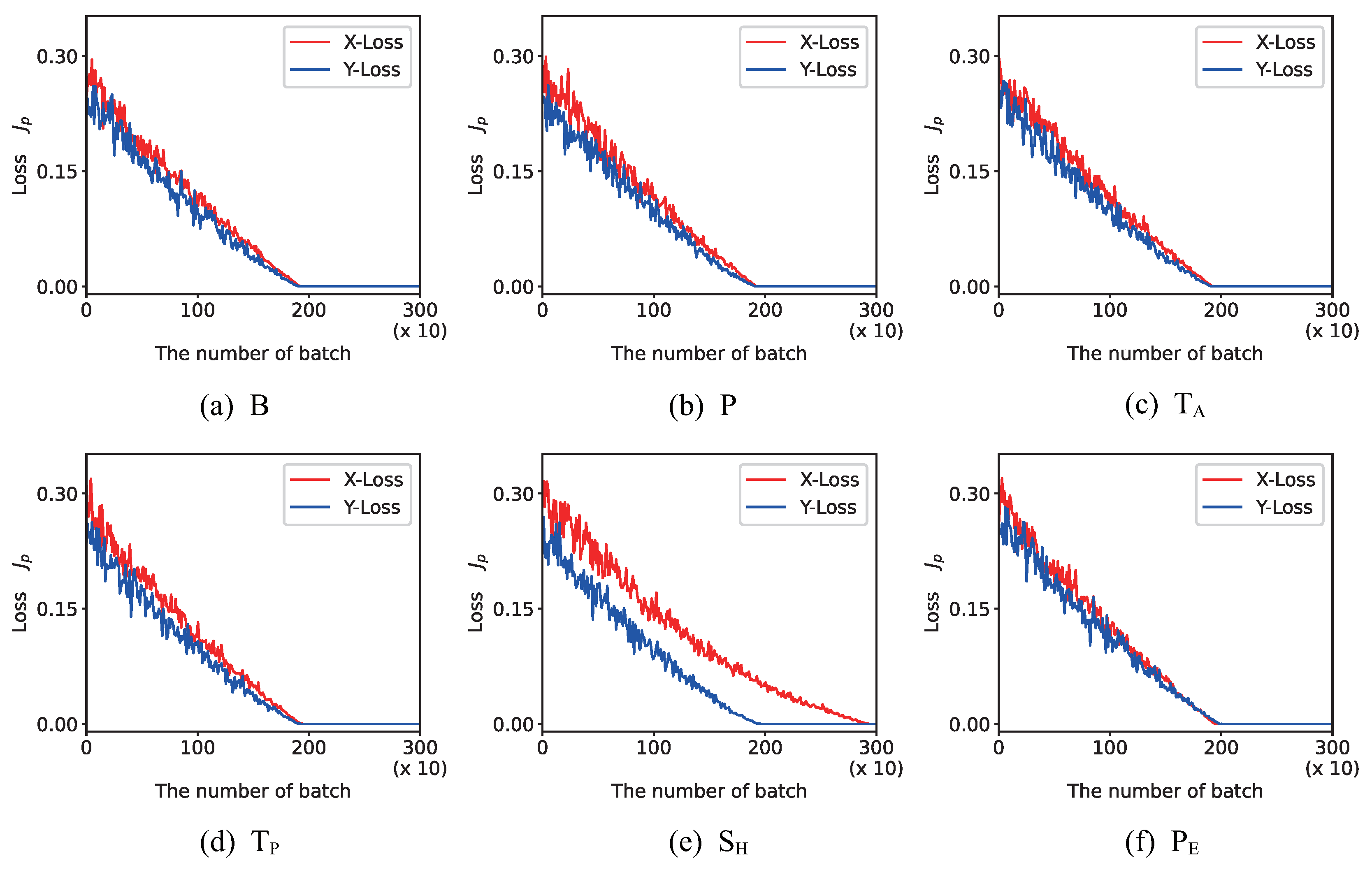
The distortion correction is first implemented for the dataset GRD. The stars in the FOV of the star tracker are evenly distributed, which is conducive to learning the global distortion of the star image. The training process is shown in Figure 7.
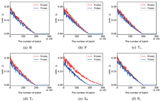
Figure 7.
The Loss for different geometric distortions of star images captured from a different area of the sky randomly: (a) B (barrel), (b) P (pincushion), (c) (tangential), (d) (thin prism), (e) (shear) and (f) (perspective). The abscissa axis is the batch size, which is 128. The initial weights of different distortions were the same.
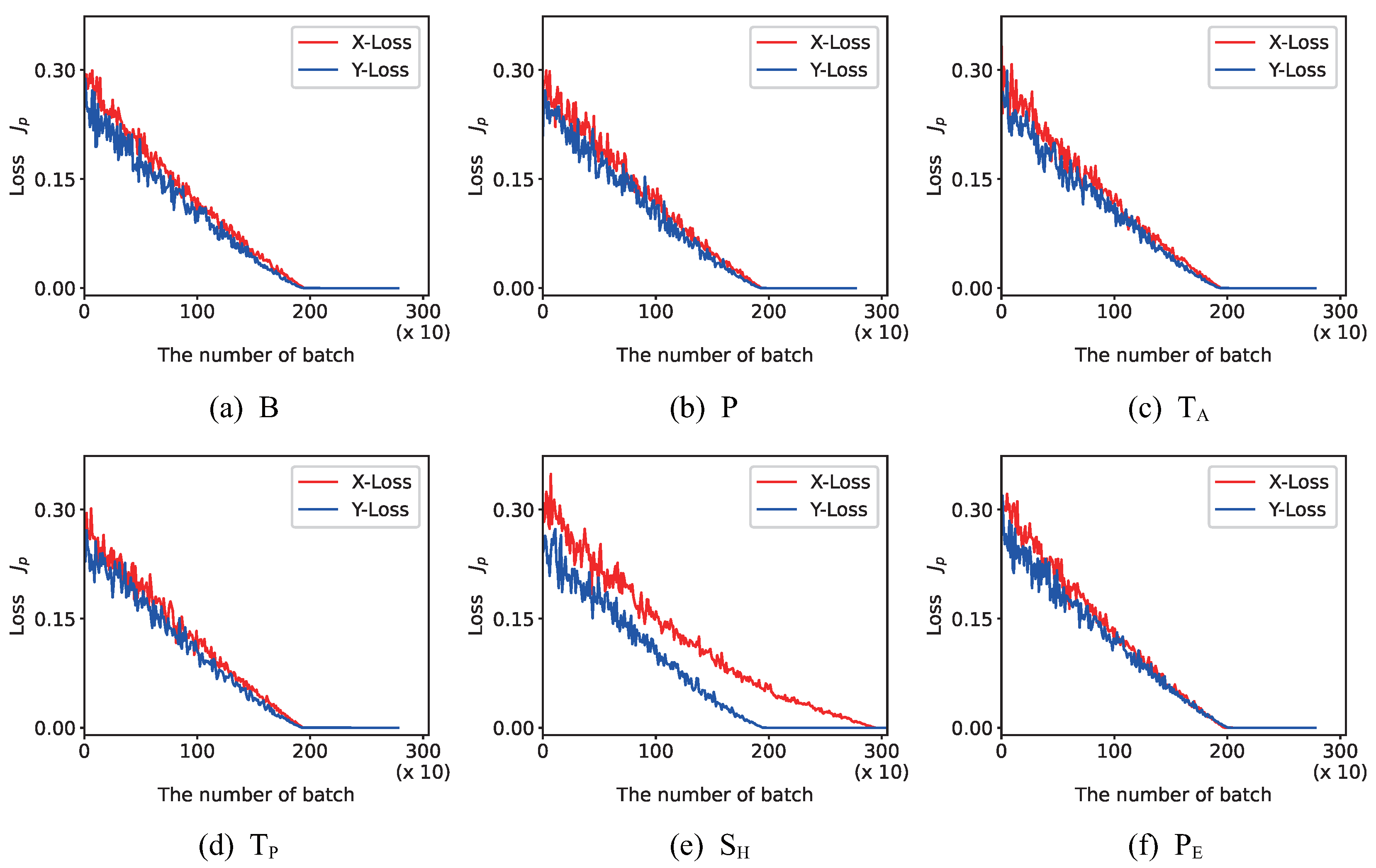
Similarly, batch learning was implemented to train the distortion model with the dataset GCD. The training process is shown in Figure 8.
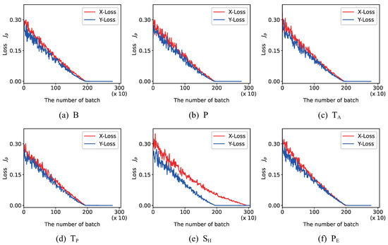
Figure 8.
The Loss for different types of geometric distortions of star images generated along the earth orbit: (a) B (barrel), (b) P (pincushion), (c) (tangential), (d) (thin prism), (e) (shear) and (f) (perspective). The abscissa axis is the batch size, which is 128. The initial weights of different distortions were the same.
The initial weights of 2DLNN were the same for the different distortions. It can be seen from Figure 7 that the initial estimation errors are different due to different distortion models. The initial weights can be randomly generated or obtained through a swarm intelligence optimization approach, such as the sparrow search algorithm (SAA [57]). After training, the estimation error of the model will converge to less than (normalized pixel).
Figure 8 considers the possibility of on-orbit implementation. We will discuss on-orbit distortion correction in Section 4.3. The ground-based experiment demonstrates that the method can fit different distortions, and the star position error can reduce to a small value after correction. The weight, trained by the ground-based experiment, can be used as the initial values of on-orbit correction. However, with different environments between ground and on-orbit, it is not easy to obtain on-orbit parameters beforehand in the laboratory. Therefore, on-orbit distortion correction is online continuation learning.
4.3. Simulation of On-Orbit Correction
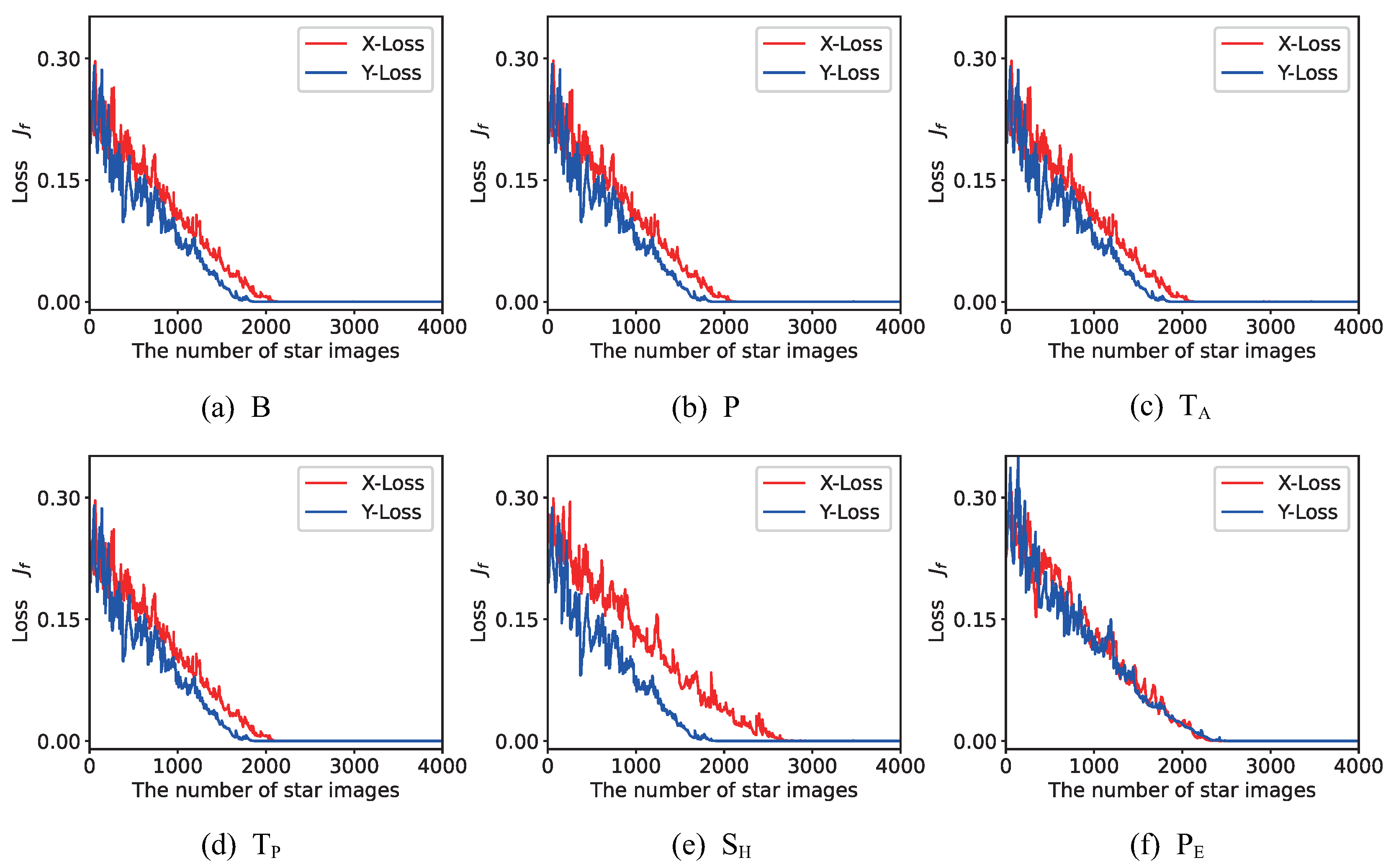
Based on the conclusion in Section 3.3.1, the dataset OD is adopted to train the on-orbit distortion model. Unlike the ground-based experiment, the on-orbit geometric distortion correction is frame-to-frame training. The on-orbit training method of 2DLNN is Equation (27), and the training process is shown in Figure 9.
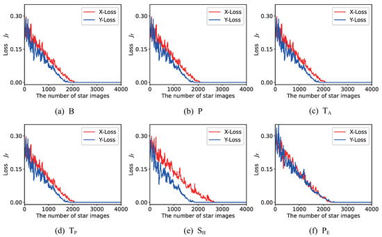
Figure 9.
The Loss for different geometric distortions of star images simulated along the starlink orbit: (a) B (barrel), (b) P (pincushion), (c) (tangential), (d) (thin prism), (e) (shear) and (f) (perspective). The initial weights of different distortions were the same.
From Figure 9, considering the resource needed for correction, about 2000 to 2200 images are needed in the rough correction. Less than 2500 star images are needed totally to achieve satisfactory correction results. Also, taking radial distortion as an example, the average running time required to train a single star image only using CPU is ms, which is suitable for on-orbit execution.
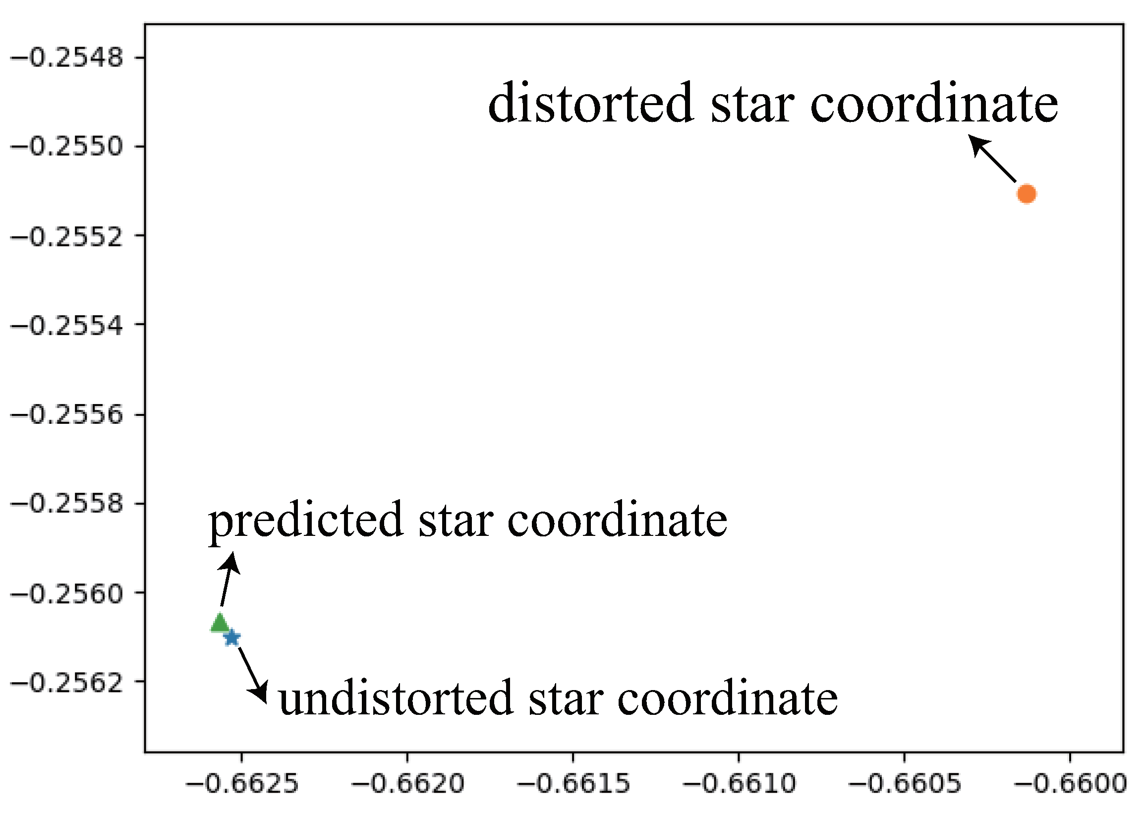
The results of the geometric distortion correction for a single star spot are shown in Figure 10, the star spot is intercepted from the radial distortion star image. For the original distortion, the distance between the observed star and the reference star is 2.683 pixels. After correction, the star position error is 0.048 pixels, and the relative error of star position can be reduced by (2.683 − 0.048)/2.683 × . It shows that the proposed geometric distortion correction algorithm is effective and accurate.

Figure 10.
Star coordinates of undistorted star spot (🟉), distorted star spot (○) and predicted star spot (△). The coordinates are all normalized to [−1, 1].
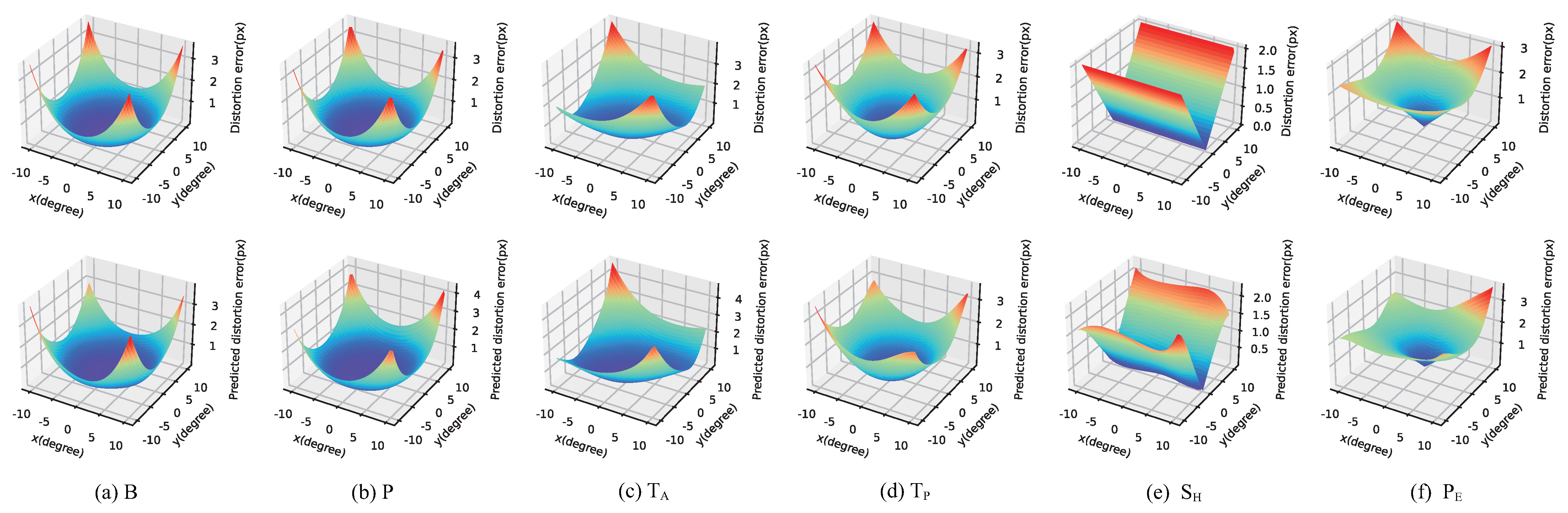
The predicted distortion flow of the image plane is shown in Figure 11. The first line is the distortion flow of the focal plane before correction, and the second line is the distortion flow learned by the proposed method. The average coordinate error of starspot is shown in Table 5. At the edge of the star image plane, the distortion caused by the optical system is about 2 pixels, while the maximum distortion of image transformation is about 3 pixels. After correction using the proposed algorithm, the star position error can be less than pixels. It indicates that the proposed method successfully predicts and corrects the star position error. In addition, for other unknown distortion models, such as distortion composed of a set of basal errors or other irregular distortions, the 2D Legendre neural network can also learn the distortion mapping.
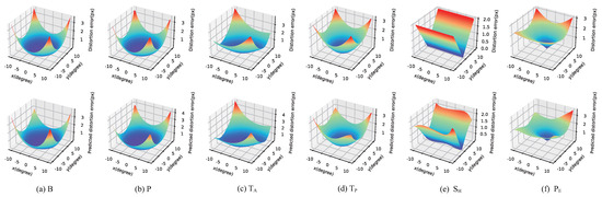
Figure 11.
The distortion error before correction and the predicted distortion flow for different distortions: (a) B (barrel), (b) P (pincushion), (c) (tangential), (d) (thin prism), (e) (shear) and (f) (perspective).
Table 5.
Average position error of different models.
4.4. Comparison with Previous Techniques
Piecewise linear mapping algorithm based on Delaunay triangulation [58], ordinary polynomial mapping method based on improved genetic algorithm [34] were applied to the geometric distortion correction of star images. The previous techniques were implemented on the radial distortion of the star tracker optical system. We only compared the distortion caused by the change of the star tracker optical system parameters, that is, radial distortion (B and P), tangential distortion (), and thin prism distortion ().
The imaging data and the star spot coordinates in the comparison experiments were the same. The average position error and execution time of three methods after correction for different distortion models are shown in Table 6, which are calculated in the direction of x and y, respectively. It can be seen that the proposed method has significant advantages in correcting the position of starspots and star images. The average execution time is quick, which is suitable for onboard implementation.
Table 6.
Average position error of different methods and average time consumed.
5. Conclusions
The star tracker is a prerequisite device to realize high-precision attitude determination for a spacecraft. However, star tracker accuracy is often influenced by optical lens machining, optical path assembly, and temperature alternation errors. Optical lens parameter changes and image distortion will have an impact on the accuracy of the star tracker. To improve the accuracy of the star tracker and the availability of star images, a novel general framework based on 2DLNN for the geometric distortion correction of on-orbit star images was proposed. An offline training method grounded on batch star images and an online training algorithm based on sequential star images were designed, respectively.
2DLNN is a single-layer neural network with fast convergence, self-learning, lifelong learning, and good adaptability, and it is suitable for on-orbit implementation. The simulations demonstrate that the average position error of distortion can be reduced to less than 0.04 px after correction. In the earth-orientation mode of the LEO satellite, the on-orbit sequential training algorithm can converge in 2500 star images under the condition of . The proposed method has the potential to become a general framework for the geometric distortion correction for star images. The method proposed in this paper can be extended to the image correction of satellite-carried optical sensors and real night observation experiments.
Author Contributions
Conceptualization, C.S., R.Z. and Y.Y.; Investigation, C.S., R.Z. and Y.Y.; Methodology, C.S. and R.Z.; Project administration, R.Z. and X.L.; Supervision, C.S. and R.Z.; Writing—review and editing, C.S. and R.Z. All authors have read and agreed to the published version of the manuscript.
Funding
This research received no external funding.
Data Availability Statement
Not applicable.
Acknowledgments
We gratefully acknowledge the support of the Innovation Academy For Microsatellites of Chinese Academy of Sciences. We also thank the engineers who helped us set up the experimental equipment. We thank LXH for her encouragement and help.
Conflicts of Interest
The authors declare no conflict of interest.
Abbreviations
The following abbreviations are used in this manuscript:
| 2DLNN | 2D Legendre Neural Network |
| B | Barrel distortion |
| P | Pincushion distortion |
| Tangential distortion | |
| Thin Prism distortion | |
| Shear transformation | |
| Perspective transformation |
Appendix A
Adam combines the advantages of AdaGrad [59] and RMSProp [60]. It comprehensively considers the first-order and second-order moment of the gradients and calculates the step of gradient updating.
The variables in the Equation (25) are as follows,
where m is the exponential moving average of gradients, is the exponential decay rate for the first moment estimates. v is the exponential moving average of square gradients, , the exponential decay rate for the second-moment estimates. and indicate that the gradient is corrected to reduce the impact of deviation on the initial stage of training. , is a very small number to prevent any division by zero in the implementation.
Appendix B
Geometric Distortion Correction Using 2D Legendre Neural Network.
| Algorithm A1 2DLNN |
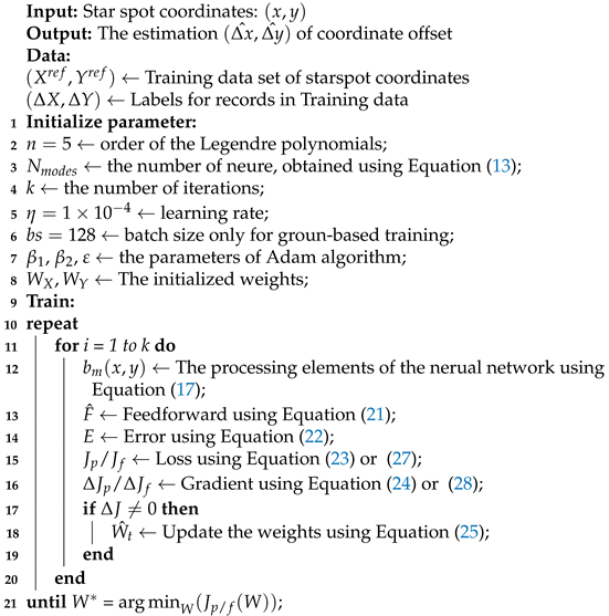 |
References
- Liebe, C.C. Accuracy performance of star trackers-a tutorial. IEEE Trans. Aerosp. Electron. Syst. 2002, 38, 587–599. [Google Scholar] [CrossRef]
- Liebe, C.C.; Gromov, K.; Meller, D.M. Toward a stellar gyroscope for spacecraft attitude determination. J. Guid. Control Dyn. 2004, 27, 91–99. [Google Scholar] [CrossRef]
- Spiller, D.; Magionami, E.; Schiattarella, V.; Curti, F.; Facchinetti, C.; Ansalone, L.; Tuozzi, A. On-orbit recognition of resident space objects by using star trackers. Acta Astronaut. 2020, 177, 478–496. [Google Scholar] [CrossRef]
- Yang, Y.; Zhang, C.; Lu, J.; Zhang, H. The Optical Reference Error Analysis and Control Method in Ground Validation System of Stellar-Inertial Integration. IEEE Sens. J. 2019, 19, 670–678. [Google Scholar] [CrossRef]
- Tan, W.; Qin, S.; Myers, R.M.; Morris, T.J.; Jiang, G.; Zhao, Y.; Wang, X.; Ma, L.; Dai, D. Centroid error compensation method for a star tracker under complex dynamic conditions. Opt. Express 2017, 25, 33559–33574. [Google Scholar] [CrossRef]
- Arnas, D.; Linares, R. Uniform Satellite Constellation Reconfiguration. J. Guid. Control Dyn. 2022, 1–14. [Google Scholar] [CrossRef]
- Arnas, D.; Linares, R. On the Theory of Uniform Satellite Constellation Reconfiguration. arXiv 2021, arXiv:2110.07817. [Google Scholar]
- Sun, T.; Xing, F.; You, Z. Optical system error analysis and calibration method of high-accuracy star trackers. Sensors 2013, 13, 4598–4623. [Google Scholar] [CrossRef]
- Wei, X.; Zhang, G.; Fan, Q.; Jiang, J.; Li, J. Star sensor calibration based on integrated modelling with intrinsic and extrinsic parameters. Measurement 2014, 55, 117–125. [Google Scholar] [CrossRef]
- Xiong, K.; Wei, X.; Zhang, G.; Jiang, J. High-accuracy star sensor calibration based on intrinsic and extrinsic parameter decoupling. Opt. Eng. 2015, 54, 34112. [Google Scholar] [CrossRef]
- Zhang, C.; Niu, Y.; Zhang, H.; Lu, J. Optimized star sensors laboratory calibration method using a regularization neural network. Appl. Opt. 2018, 57, 1067–1074. [Google Scholar] [CrossRef]
- Ye, T.; Zhang, X.; Xie, J.F. Laboratory calibration of star sensors using a global refining method. J. Opt. Soc. Am. Opt. Image Sci. Vis. 2018, 35, 1674–1684. [Google Scholar] [CrossRef]
- Fan, Q.; He, K.; Wang, G. Star sensor calibration with separation of intrinsic and extrinsic parameters. Opt. Express 2020, 28, 21318–21335. [Google Scholar] [CrossRef]
- Liu, H.B.; Tan, J.C.; Hao, Y.C.; Hui, J.; Wei, T.; Yang, J.K. Effect of ambient temperature on star sensor measurement accuracy. Opto-Electron. Eng. 2008, 35, 40. [Google Scholar]
- Liwei, L.; Zijun, Z.; Qian, X.; Liang, W. Study on BP neural network model of optical system parameters based on temperature variation. In Proceedings of the 2019 14th IEEE International Conference on Electronic Measurement & Instruments (ICEMI), Changsha, China, 1–3 November 2019; pp. 930–935. [Google Scholar]
- Liang, W.; Chao, H.; Kaixuan, Z.; Qian, X. On-Orbit Calibration of Star Sensor under Temperature Variation. In Proceedings of the 2021 6th International Symposium on Computer and Information Processing Technology (ISCIPT), Changsha, China, 11–13 June 2021; pp. 532–535. [Google Scholar]
- Wang, J.-Q.; Liu, H.-B.; Tan, J.-C.; Yang, J.-K.; Jia, H.; Li, X.-J. Autonomous on-orbit calibration of a star tracker camera. Opt. Eng. 2011, 50, 023604. [Google Scholar] [CrossRef]
- Zhang, H.; Niu, Y.; Lu, J.; Zhang, C.; Yang, Y. On-orbit calibration for star sensors without priori information. Opt. Express 2017, 25, 18393–18409. [Google Scholar] [CrossRef]
- Curti, F.; Spiller, D.; Ansalone, L.; Becucci, S.; Procopio, D.; Boldrini, F.; Fidanzati, P.; Sechi, G. High angular rate determination algorithm based on star sensing. Adv. Astronaut. Sci. Guid. Navig. Control. 2015, 154, 12. [Google Scholar]
- Schiattarella, V.; Spiller, D.; Curti, F. Star identification robust to angular rates and false objects with rolling shutter compensation. Acta Astronaut. 2020, 166, 243–259. [Google Scholar] [CrossRef]
- He, L.; Ma, Y.; Zhao, R.; Hou, Y.; Zhu, Z. High Update Rate Attitude Measurement Method of Star Sensors Based on Star Point Correction of Rolling Shutter Exposure. Sensors 2021, 21, 5724. [Google Scholar] [CrossRef]
- Samaan, M.A.; Griffith, T.S.; Singla, P.; Junkins, J.L. Autonomous on-Orbit Calibration Of Star Trackers. In Proceedings of the Core Technologies for Space Systems Conference (Communication and Navigation Session), New York, NY, USA, 5–16 May 2001. [Google Scholar]
- Singla, P.; Griffith, D.T.; Crassidis, J.L.; Junkins, J.L. Attitude determination and autonomous on-orbit calibration of star tracker for the gifts mission. Adv. Astronaut. Sci. 2002, 112, 19–38. [Google Scholar]
- Yuan, Y.H.; Geng, Y.H.; Chen, X.Q. On-orbit calibration of star sensor with landmark. J. Harbin Univ. Commer. (Natural Sci. Ed.) 2008, 24, 448–453. [Google Scholar]
- Tan, W.; Dai, D.; Wu, W.; Wang, X.; Qin, S. A Comprehensive Calibration Method for a Star Tracker and Gyroscope Units Integrated System. Sensors 2018, 18, 3106. [Google Scholar] [CrossRef] [PubMed]
- Yang, Z.; Zhu, X.; Cai, Z.; Chen, W.; Yu, J. A real-time calibration method for the systematic errors of a star sensor and gyroscope units based on the payload multiplexed. Optik 2021, 225, 165731. [Google Scholar] [CrossRef]
- Zhou, F.; Ye, T.; Chai, X.; Wang, X.; Chen, L. Novel autonomous on-orbit calibration method for star sensors. Opt. Lasers Eng. 2015, 67, 135–144. [Google Scholar] [CrossRef]
- Wang, S.; Geng, Y.; Jin, R. A Novel Error Model of Optical Systems and an On-Orbit Calibration Method for Star Sensors. Sensors 2015, 15, 31428–31441. [Google Scholar] [CrossRef]
- Medaglia, E. Autonomous on-orbit calibration of a star tracker. In Proceedings of the 2016 IEEE Metrology for Aerospace (MetroAeroSpace), Florence, Italy, 22–23 June 2016; pp. 456–461. [Google Scholar]
- Wu, L.; Xu, Q.; Heikkilä, J.; Zhao, Z.; Liu, L.; Niu, Y. A Star Sensor On-Orbit Calibration Method Based on Singular Value Decomposition. Sensors 2019, 19, 3301. [Google Scholar] [CrossRef]
- Liang, W.; Zijun, Z.; Qian, X.; Liwei, L. Star sensor on-orbit calibration based on multiple calibration targets. In Proceedings of the 2019 14th IEEE International Conference on Electronic Measurement & Instruments (ICEMI), Changsha, China, 1–3 November 2019; pp. 1402–1409. [Google Scholar]
- Jin, H.; Mao, X.; Li, X. Research on Star Tracker On-orbit Low Spatial Frequency Error Compensation. Acta Photonica Sin. 2020, 49, 0112005. [Google Scholar] [CrossRef]
- Wu, L.; Xu, Q.; Han, C.; Zhang, K. An On-Orbit Calibration Method of Star Sensor Based on Angular Distance Subtraction. IEEE Photonics J. 2021, 13, 1–13. [Google Scholar] [CrossRef]
- Wei, Q.; Jiancheng, F.; Weina, Z. A method of optimization for the distorted model of star map based on improved genetic algorithm. Aerosp. Sci. Technol. 2011, 15, 103–107. [Google Scholar] [CrossRef]
- Yuan, L.; Ruida, X.; Lin, Z.; Hao, Y. Machine Learning based on-orbit distortion calibration technique for large field-of-view star tracker. Infrared Laser Eng. 2016, 45, 282–290. [Google Scholar]
- Goshtasby, A. Image registration by local approximation methods. Image Vis. Comput. 1988, 6, 255–261. [Google Scholar] [CrossRef]
- Wahba, G. A least squares estimate of satellite attitude. SIAM Rev. 1965, 7, 409. [Google Scholar] [CrossRef]
- Bar-Itzhack, I.Y. REQUEST-A recursive QUEST algorithm for sequential attitude determination. J. Guid. Control. Dyn. 1996, 19, 1034–1038. [Google Scholar] [CrossRef]
- Wei, M.S.; Xing, F.; You, Z. A real-time detection and positioning method for small and weak targets using a 1D morphology-based approach in 2D images. Light. Sci. Appl. 2018, 7, 18006. [Google Scholar] [CrossRef] [PubMed]
- Brown, D.C. Decentering distortion of lenses. Photogramm. Eng. Remote Sens. 1966, 31, 444–462. [Google Scholar]
- Liu, Y.; Cheng, D.; Wang, Q.; Hou, Q.; Gu, L.; Chen, H.; Yang, T.; Wang, Y. Optical distortion correction considering radial and tangential distortion rates defined by optical design. Results Opt. 2021, 3, 100072. [Google Scholar] [CrossRef]
- Liang, X.; Zhou, J.; Ma, W. Method of distortion and pointing correction of a ground-based telescope. Appl. Opt. 2019, 58, 5136–5142. [Google Scholar] [CrossRef]
- Chen, X.; Xing, F.; You, Z.; Zhong, X.; Qi, K. On-Orbit High-Accuracy Geometric Calibration for Remote Sensing Camera Based on Star Sources Observation. IEEE Trans. Geosci. Remote Sens. 2021, 60, 1–11. [Google Scholar] [CrossRef]
- Service, M.; Lu, J.R.; Campbell, R.; Sitarski, B.N.; Ghez, A.M.; Anderson, J. A New Distortion Solution for NIRC2 on the Keck II Telescope. Publ. Astron. Soc. Pac. 2016, 128, 095004. [Google Scholar] [CrossRef]
- Ye, J.; Gao, Z.; Wang, S.; Cheng, J.; Wang, W.; Sun, W. Comparative assessment of orthogonal polynomials for wavefront reconstruction over the square aperture. J. Opt. Soc. Am. A 2014, 31, 2304–2311. [Google Scholar] [CrossRef]
- Yang, S.S.; Tseng, C.S. An orthogonal neural network for function approximation. IEEE Trans. Syst. Man, Cybern. Part B Cybern. 1996, 26, 779–785. [Google Scholar] [CrossRef] [PubMed]
- Francois, B. Orthogonal considerations in the design of neural networks for function approximation. Math. Comput. Simul. 1996, 41, 95–108. [Google Scholar] [CrossRef]
- Kingma, D.P.; Ba, J. Adam: A method for stochastic optimization. arXiv 2014, arXiv:1412.6980. [Google Scholar]
- Zhang, G. Star Identification: Methods, Techniques and Algorithms; Springer: Berlin/Heidelberg, Germany, 2016. [Google Scholar]
- Sun, T.; Xing, F.; Bao, J.; Ji, S.; Li, J. Suppression of stray light based on energy information mining. Appl. Opt. 2018, 57, 9239–9245. [Google Scholar] [CrossRef]
- Shi, C.; Zhang, R.; Yu, Y.; Sun, X.; Lin, X. A SLIC-DBSCAN Based Algorithm for Extracting Effective Sky Region from a Single Star Image. Sensors 2021, 21, 5786. [Google Scholar] [CrossRef] [PubMed]
- Wan, X.; Wang, G.; Wei, X.; Li, J.; Zhang, G. ODCC: A Dynamic Star Spots Extraction Method for Star Sensors. IEEE Trans. Instrum. Meas. 2021, 70, 1–14. [Google Scholar] [CrossRef]
- Samirbhai, M.D.; Chen, S. A Star Pattern Recognition Technique Based on the Binary Pattern Formed from the FFT Coefficients. In Proceedings of the 2018 IEEE International Symposium on Circuits and Systems (ISCAS), Florence, Italy, 27–30 May 2018; pp. 1–5. [Google Scholar]
- Mehta, D.S.; Chen, S.; Low, K.S. A rotation-invariant additive vector sequence based star pattern recognition. IEEE Trans. Aerosp. Electron. Syst. 2018, 55, 689–705. [Google Scholar] [CrossRef]
- Xingzhe, S.; Rui, Z.; Chenguang, S.; Xiaodong, L. Star Identification Algorithm Based on Dynamic Angle Matching. Acta Opt. Sin. 2021, 41, 1610001. [Google Scholar]
- Shuster, M.D. Algorithms for Determining Optimal Attitude Solutions; Computer Sciences Corporation: Tysons Corner, VA, USA, 1978. [Google Scholar]
- Xue, J.; Shen, B. A novel swarm intelligence optimization approach: Sparrow search algorithm. Syst. Sci. Control Eng. 2020, 8, 22–34. [Google Scholar] [CrossRef]
- Goshtasby, A. Piecewise linear mapping functions for image registration. Pattern Recognit. 1986, 19, 459–466. [Google Scholar] [CrossRef]
- Duchi, J.; Hazan, E.; Singer, Y. Adaptive subgradient methods for online learning and stochastic optimization. J. Mach. Learn. Res. 2011, 12, 2121–2159. [Google Scholar]
- Hinton, G.; Srivastava, N.; Swersky, K. Neural networks for machine learning lecture 6a overview of mini-batch gradient descent. Cited On 2012, 14, 2. [Google Scholar]
Publisher’s Note: MDPI stays neutral with regard to jurisdictional claims in published maps and institutional affiliations. |
© 2022 by the authors. Licensee MDPI, Basel, Switzerland. This article is an open access article distributed under the terms and conditions of the Creative Commons Attribution (CC BY) license (https://creativecommons.org/licenses/by/4.0/).