
Deriving 3-D Surface Deformation Time Series with Strain Model and Kalman Filter from GNSS and InSAR Data


Abstract
:
1. Introduction
2. Methods
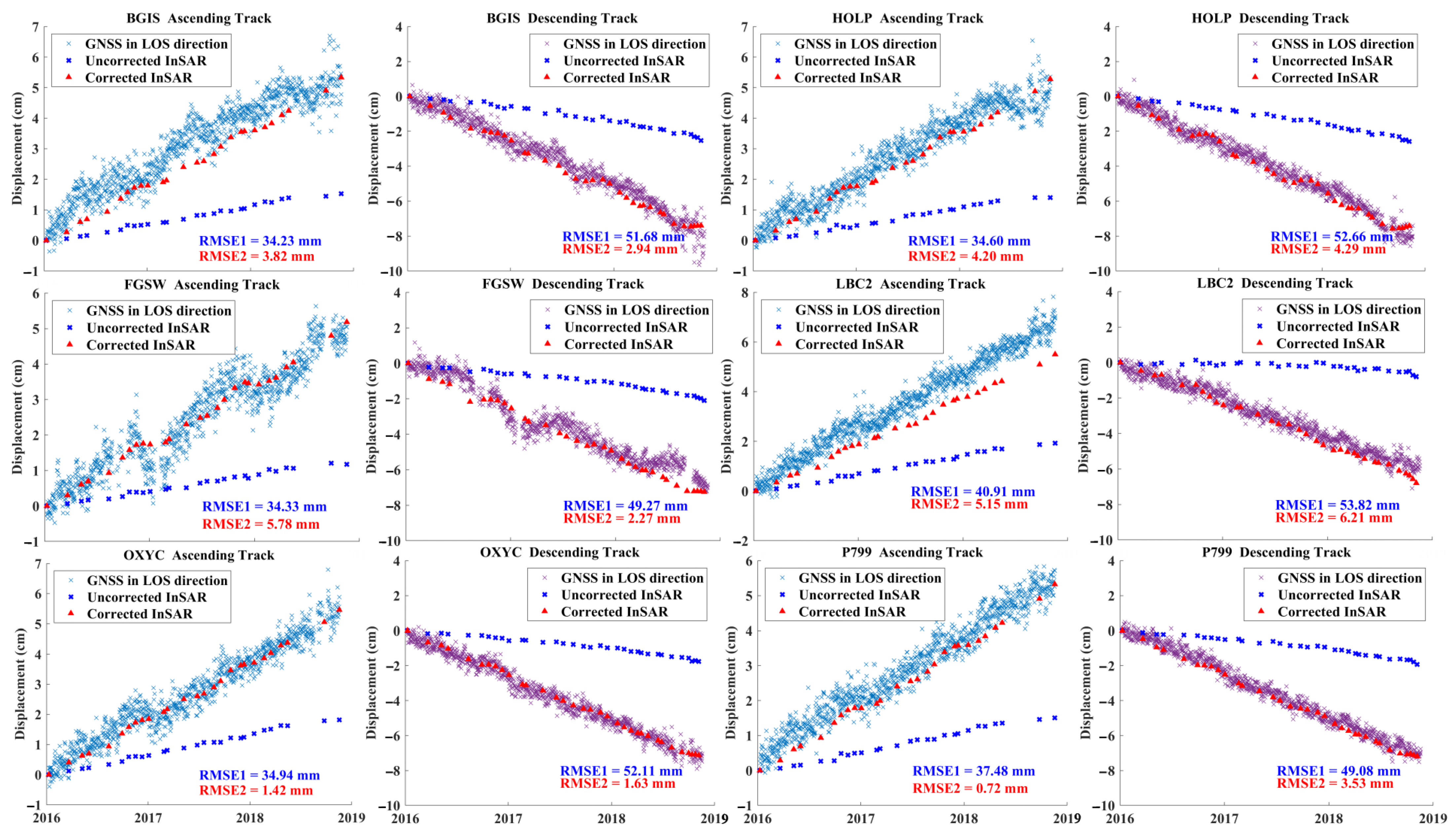
2.1. Correction of InSAR Observations
- Project the GNSS 3-D displacements corresponding to the InSAR acquisition moments to the LOS directionwhere , and are the GNSS displacements in the east–west, north–south and up–down directions, respectively. The unit project vector . denotes the incidence angle of the satellite site and represents the heading angle, that is, the clockwise angle between the north and the flight of the satellite. Through Equation (1), the 3-D GNSS displacements are projected to the LOS direction .
- The polynomial fitting can establish the relationship between GNSS projection values and InSAR observations at the same location and moment. Assuming a second-order polynomial fit, the relationship between the two observations can be expressed aswhere a, b and c are the fitting coefficients, and is the InSAR observation in the LOS direction. It can be seen that as long as the number of GNSS points in the study area is greater than three, the optimal polynomial coefficients can be obtained through the least squares method. Of course, the more GNSS points involved in the fitting, the more accurate the coefficients will be.
- Correct the InSAR observations for each pixel using the polynomial coefficients obtained. The above steps will be performed independently for each observation moment of the ascending and descending track InSAR datasets.
2.2. State Equation
2.3. Observation Equation
2.4. SM-Kalman
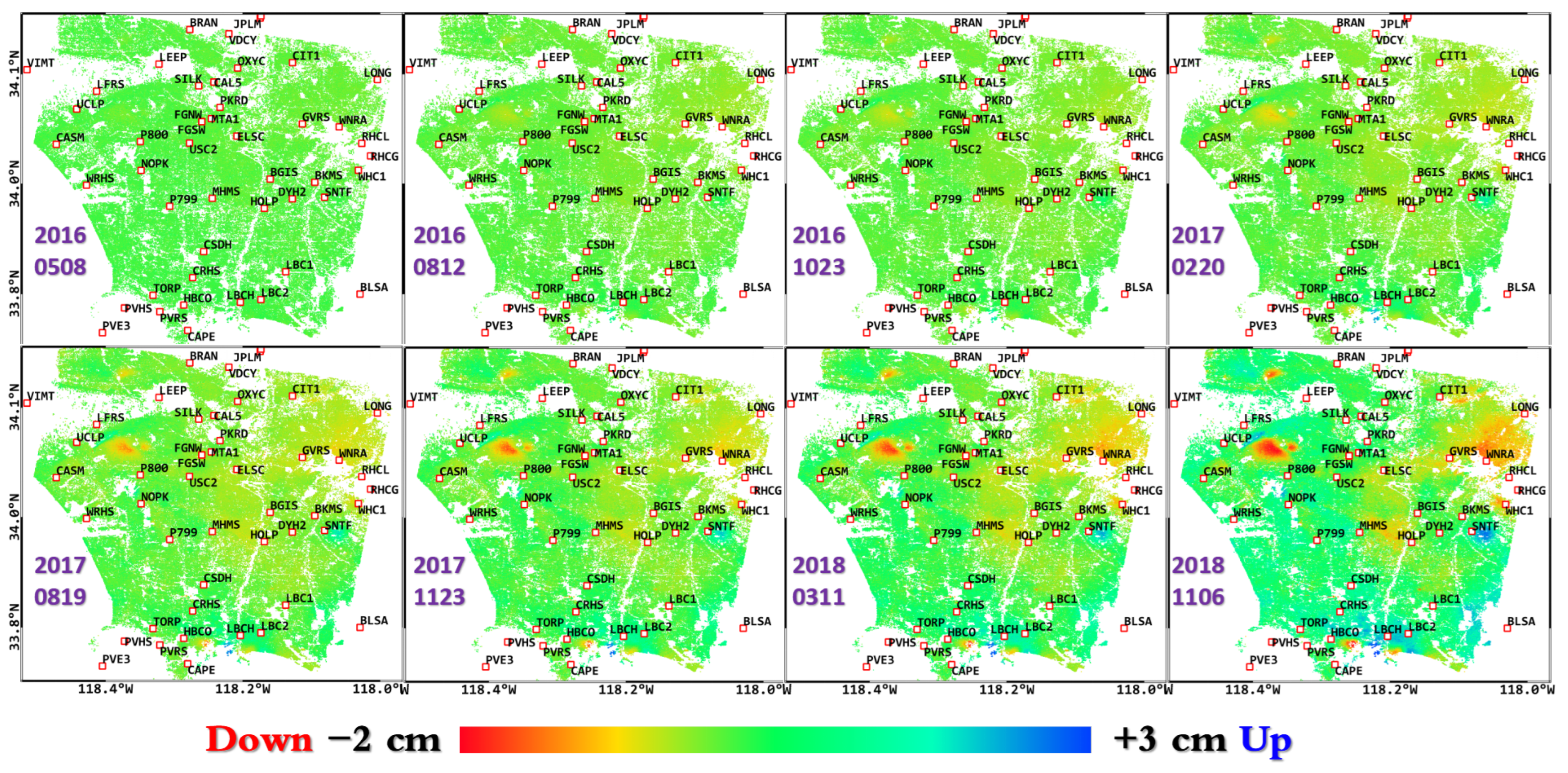
3. Results
3.1. InSAR and GNSS Results
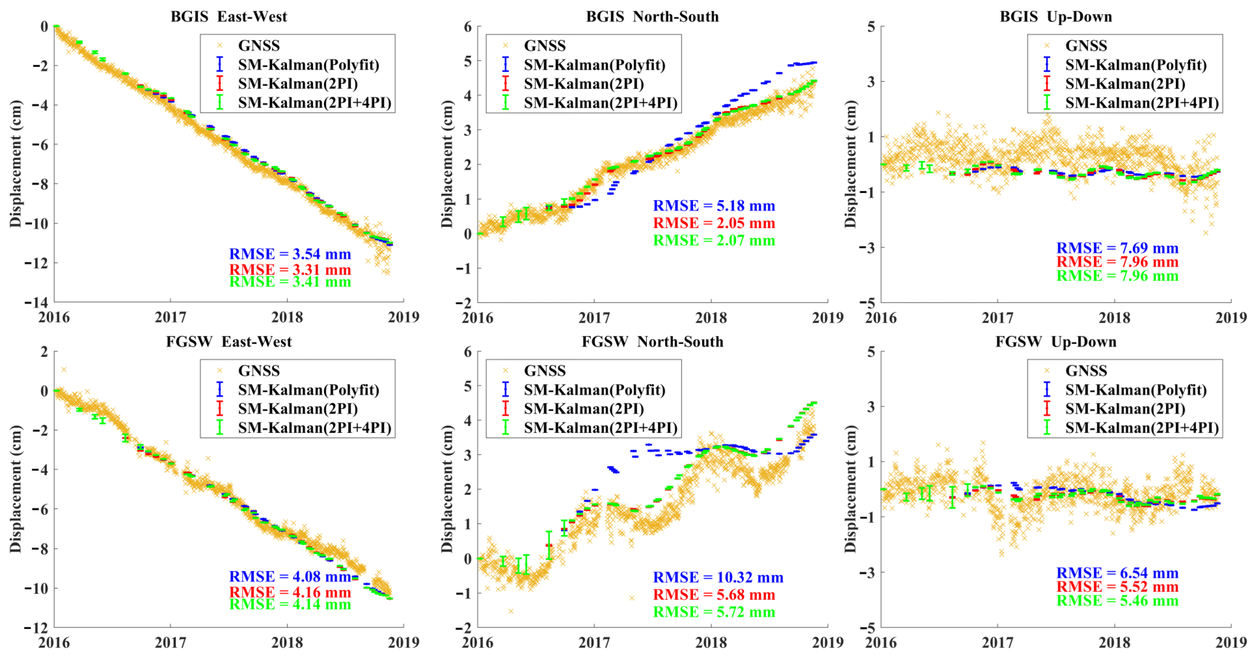
3.2. 3-D Deformation Time Series
4. Discussion
5. Conclusions
Author Contributions
Funding
Data Availability Statement
Acknowledgments
Conflicts of Interest
References
- Zha, X.; Fu, R.; Dai, Z.; Jing, P.; Ni, S.; Huang, J. Applying insar technique to accurately relocate the epicentre for the 1999 Ms = 5.6 kuqa earthquake in Xinjiang Province, China. Geophys. J. Int. 2009, 176, 107–112. [Google Scholar] [CrossRef]
- Li, S.; Chen, G.; Tao, T.; He, P.; Ding, K.; Zou, R.; Li, J.; Wang, Q. The 2019 MW 6.4 and MW 7.1 Ridgecrest earthquake sequence in eastern California: Rupture on a conjugate fault structure revealed by GPS and Insar Measurements. Geophys. J. Int. 2020, 221, 1651–1666. [Google Scholar] [CrossRef]
- Liang, H.; Li, X.; Chen, R. Mapping surface deformation over Tatun volcano group, northern Taiwan using multitemporal insar. IEEE J. Sel. Top. Appl. Earth Obs. Remote Sens. 2021, 14, 2087–2095. [Google Scholar] [CrossRef]
- Leick, A.; Rapoport, L.; Tatarnikov, D. GPS Satellite Surveying; Wiley: Hoboken, NJ, USA, 2015. [Google Scholar]
- Jin, S.; Feng, G.; Gleason, S. Remote sensing using GNSS signals: Current status and Future Directions. Adv. Space Res. 2011, 47, 1645–1653. [Google Scholar] [CrossRef]
- Hu, J.; Li, Z.; Ding, X.L.; Zhu, J.; Zhang, L.; Sun, Q. Resolving three-dimensional surface displacements from insar measurements: A Review. Earth-Sci. Rev. 2014, 133, 1–17. [Google Scholar] [CrossRef]
- Wang, Z.; Liu, G.; Hu, L.; Tao, Q.; Yu, S. Method for determining weight matrix for resolving three-dimensional surface deformation using multi-los D-Insar Technology. Int. J. Appl. Earth Obs. Geoinf. 2020, 88, 102062. [Google Scholar] [CrossRef]
- Gudmundsson, S.; Carstensen, J.M.; Sigmundsson, F. Unwrapping ground displacement signals in satellite radar interferograms with aid of GPS data and MRF regularization. IEEE Trans. Geosci. Remote Sens. 2002, 40, 1743–1754. [Google Scholar] [CrossRef]
- Samsonov, S.; Tiampo, K. Analytical optimization of a DINSAR and GPS dataset for derivation of three-dimensional surface motion. IEEE Geosci. Remote Sens. Lett. 2006, 3, 107–111. [Google Scholar] [CrossRef]
- Hu, J.; Li, Z.; Zhu, J.; Ding, X.; Wang, C.; Feng, G.; Sun, Q. Measuring three-dimensional surface displacements from combined InSAR and GPS data based on BFGS method. Chin. J. Geophys. 2013, 56, 117–126. [Google Scholar]
- Shi, G. qiang; He, X. feng; Xiao, R. ya Acquiring three-dimensional deformation of Kilauea’s south flank from GPS and Dinsar integration based on the ant colony optimization. IEEE Geosci. Remote Sens. Lett. 2015, 12, 2506–2510. [Google Scholar]
- Ji, P.; Lv, X.; Dou, F.; Yun, Y. Fusion of GPS and InSAR data to derive robust 3D deformation maps based on MRF L1-regularization. Remote Sens. Lett. 2019, 11, 204–213. [Google Scholar] [CrossRef]
- Hu, J.; Li, Z.; Sun, Q.; Zhu, J.; Ding, X. Three-Dimensional Surface Displacements From InSAR and GPS Measurements With Variance Component Estimation. IEEE Geosci. Remote Sens. Lett. 2012, 9, 754–758. [Google Scholar]
- Song, X.; Jiang, Y.; Shan, X.; Qu, C. Deriving 3D coseismic deformation field by combining GPS and InSAR data based on the elastic dislocation model. Int. J. Appl. Earth Obs. Geoinf. 2017, 57, 104–112. [Google Scholar] [CrossRef]
- Ji, P.; Lv, X.; Chen, Q.; Sun, G.; Yao, J. Applying InSAR AND GNSS data to Obtain 3-D Surface Deformations based on Iterated Almost Unbiased estimation and Laplacian Smoothness Constraint. IEEE J. Sel. Top. Appl. Earth Obs. Remote Sens. 2021, 14, 337–349. [Google Scholar] [CrossRef]
- Guglielmino, F.; Nunnari, G.; Puglisi, G.; Spata, A. Simultaneous and Integrated Strain Tensor Estimation From Geodetic and Satellite Deformation Measurements to Obtain Three-Dimensional Displacement Maps. IEEE Trans. Geosci. Remote Sens. 2011, 49, 1815–1826. [Google Scholar] [CrossRef]
- Allmendinger, R.W.; Cardozo, N.; Fisher, D.W. Structural Geology Algorithms: Vectors and Tensors; Cambridge University Press: Cambridge, UK, 2012. [Google Scholar]
- Ji, P.; Lv, X.; Yao, J.; Sun, G. A New Method to Obtain 3-D Surface Deformations From InSAR and GNSS Data With Genetic Algorithm and Support Vector Machine. IEEE Geosci. Remote Sens. Lett. 2021, 19, 1–5. [Google Scholar] [CrossRef]
- Pepe, A.; Solaro, G.; Calo, F.; Dema, C. A Minimum Acceleration Approach for the Retrieval of Multiplatform InSAR Deformation Time Series. IEEE J. Sel. Top. Appl. Earth Obs. Remote Sens. 2016, 9, 3883–3898. [Google Scholar] [CrossRef]
- Yang, Z.; Li, Z.; Zhu, J.; Preusse, A.; Hu, J.; Feng, G.; Papst, M. Time-Series 3-D Mining-Induced Large Displacement Modeling and Robust Estimation From a Single-Geometry SAR Amplitude Data Set. IEEE Trans. Geosci. Remote Sens. 2018, 56, 3600–3610. [Google Scholar] [CrossRef]
- Zhao, Q.; Ma, G.; Wang, Q.; Yang, T.; Liu, M.; Gao, W.; Falabella, F.; Mastro, P.; Pepe, A. Generation of long-term InSAR ground displacement time-series through a novel multi-sensor data merging technique: The case study of the Shanghai coastal area. ISPRS J. Photogramm. Remote Sens. 2019, 154, 10–27. [Google Scholar] [CrossRef]
- Hu, J.; Ding, X.; Li, Z.; Zhu, J.; Sun, Q.; Zhang, L. Kalman-Filter-Based Approach for Multisensor, Multitrack, and Multitemporal InSAR. IEEE Trans. Geosci. Remote Sens. 2013, 51, 4226–4239. [Google Scholar] [CrossRef]
- Samsonov, S.; d’Oreye, N. Multidimensional time-series analysis of ground deformation from multiple InSAR data sets applied to Virunga Volcanic Province. Geophys. J. Int. 2012, 191, 1095–1108. [Google Scholar]
- Liu, J.; Hu, J.; Li, Z.; Sun, Q.; Ma, Z.; Zhu, J.; Wen, Y. Dynamic estimation of multi-dimensional deformation time series from Insar based on Kalman filter and strain model. IEEE Trans. Geosci. Remote Sens. 2022, 60, 1–16. [Google Scholar] [CrossRef]
- Konak, H.; Küreç Nehbit, P.; Karaöz, A.; Cerit, F. Interpreting deformation results of geodetic network points using the strain models based on different estimation methods. Int. J. Eng. Geosci. 2020, 5, 49–59. [Google Scholar] [CrossRef]
- He, X.; Montillet, J.-P.; Fernandes, R.; Bos, M.; Yu, K.; Hua, X.; Jiang, W. Review of current GPS methodologies for producing accurate time series and their error sources. J. Geodyn. 2017, 106, 12–29. [Google Scholar] [CrossRef]
- Neely, W.R.; Borsa, A.A.; Silverii, F. Ginsar: A CGPS correction for enhanced Insar Time Series. IEEE Trans. Geosci. Remote Sens. 2020, 58, 136–146. [Google Scholar] [CrossRef]
- Ferretti, A.; Prati, C.; Rocca, F. Nonlinear subsidence rate estimation using permanent scatterers in differential SAR interferometry. IEEE Trans. Geosci. Remote Sens. 2000, 38, 2202–2212. [Google Scholar] [CrossRef]
- Jia, H.; Liu, L. A technical review on persistent scatterer interferometry. J. Mod. Transp. 2016, 24, 153–158. [Google Scholar] [CrossRef]
- Simon, D. Optimal State Estimation: Kalman, H Infinity, and Nonlinear Approaches; John Wiley & Sons: Hoboken, NJ, USA, 2006. [Google Scholar]
- Anderssohn, J.; Motagh, M.; Walter, T.R.; Rosenau, M.; Kaufmann, H.; Oncken, O. Surface deformation time series and source modeling for a volcanic complex system based on satellite wide swath and image mode interferometry: The Lazufre System, Central Andes. Remote Sens. Environ. 2009, 113, 2062–2075. [Google Scholar] [CrossRef]
- Cressie, N. Spatial prediction and ordinary kriging. Math. Geol. 1989, 21, 493–494. [Google Scholar] [CrossRef]
- Davis, J.L.; Wernicke, B.P.; Tamisiea, M.E. On Seasonal signals in geodetic time series. J. Geophys. Res. Solid Earth 2012, 117. [Google Scholar] [CrossRef]
- Hu, J.; Wang, Q.; Li, Z.; Zhao, R.; Sun, Q. Investigating the Ground Deformation and Source Model of the Yangbajing Geothermal Field in Tibet, China with the WLS InSAR Technique. Remote Sens. 2016, 8, 191. [Google Scholar] [CrossRef]
- Pietrantonio, G.; Riguzzi, F. Three-dimensional strain tensor estimation by GPS observations: Methodological Aspects and Geophysical Applications. J. Geodyn. 2004, 38, 1–18. [Google Scholar] [CrossRef]
- Liu, J.; Hu, J.; Li, Z.; Zhu, J.; Sun, Q.; Gan, J. A Method for Measuring 3-D Surface Deformations with InSAR Based on Strain Model and Variance Component Estimation. IEEE Trans. Geosci. Remote Sens. 2018, 56, 239–250. [Google Scholar] [CrossRef]
- Segall, P. Earthquake and Volcano Deformation; Princeton University Press: Princeton, NJ, USA, 2010. [Google Scholar]
- Goudarzi, M.A.; Cocard, M.; Santerre, R. GeoStrain: An open source software for calculating crustal strain rates. Comput. & Geosci. 2015, 82, 1–12. [Google Scholar]
- Shen, Z.; Jackson, D.; Ge, B. Crustal deformation across and beyond the Los Angeles Basin from Geodetic Measurements. J. Geophys. Res. Solid Earth 1996, 101, 27957–27980. [Google Scholar] [CrossRef]
- Li, Z.; Ding, X.; Huang, C.; Zhu, J.; Chen, Y. Improved filtering parameter determination for the Goldstein Radar Interferogram Filter. ISPRS J. Photogramm. Remote Sens. 2008, 63, 621–634. [Google Scholar] [CrossRef]
- Jiang, H.; Balz, T.; Cigna, F.; Tapete, D. Land subsidence in Wuhan revealed using a non-linear PSINSAR approach with long time series of Cosmo-SkyMed Sar Data. Remote Sens. 2021, 13, 1256. [Google Scholar] [CrossRef]
- Costantini, M. A novel phase unwrapping method based on network programming. IEEE Trans. Geosci. Remote Sens. 1998, 36, 813–821. [Google Scholar] [CrossRef]
- Bawden, G.W.; Thatcher, W.; Stein, R.S.; Hudnut, K.W.; Peltzer, G. Tectonic contraction across Los Angeles after removal of groundwater pumping effects. Nature 2001, 412, 812–815. [Google Scholar] [CrossRef]
- Watson, K.M.; Bock, Y.; Sandwell, D.T. Satellite interferometric observations of displacements associated with seasonal groundwater in the Los Angeles Basin. J. Geophys. Res. Solid Earth 2002, 107, ETG8-1–ETG8-15. [Google Scholar] [CrossRef]
- Argus, D.F.; Heflin, M.B.; Peltzer, G.; Crampé, F.; Webb, F.H. Interseismic strain accumulation and anthropogenic motion in metropolitan Los Angeles. J. Geophys. Res. Solid Earth 2005, 110, B04401. [Google Scholar] [CrossRef]
- Zoback, M.D.; Zoback, M.L.; Mount, V.S.; Suppe, J.; Eaton, J.P.; Healy, J.H.; Oppenheimer, D.; Reasenberg, P.; Jones, L.; Raleigh, C.B.; et al. New evidence on the state of stress of the San Andreas Fault System. Science 1987, 238, 1105–1111. [Google Scholar] [CrossRef] [PubMed]
- Hu, J.; Ding, X.L.; Li, Z.W.; Zhang, L.; Zhu, J.J.; Sun, Q.; Gao, G.J. Vertical and horizontal displacements of Los Angeles from Insar and GPS time series analysis: Resolving tectonic and anthropogenic motions. J. Geodyn. 2016, 99, 27–38. [Google Scholar] [CrossRef]
- Lu, Z.; Danskin, W.R. Insar analysis of natural recharge to define structure of a ground-water basin, San Bernardino, California. Geophys. Res. Lett. 2001, 28, 2661–2664. [Google Scholar] [CrossRef]
- Impact of Drought on Water Demand in Los Angeles, USA. Available online: https://uu.diva-portal.org/smash/get/diva2:1581142/FULLTEXT01.pdf (accessed on 29 May 2022).
- Strauss, E.G.; Kafatos, M.C.; Kim, S.H.; Nghiem, S.V.; Pal, J. Applying remote sensing to urban ecosystem dynamics: Opportunities for understanding and managing the Ballona Wetland System in Los Angeles. In Proceedings of the 2017 IEEE International Geoscience and Remote Sensing Symposium (IGARSS), Fort Worth, TX, USA, 23–28 July 2017. [Google Scholar]


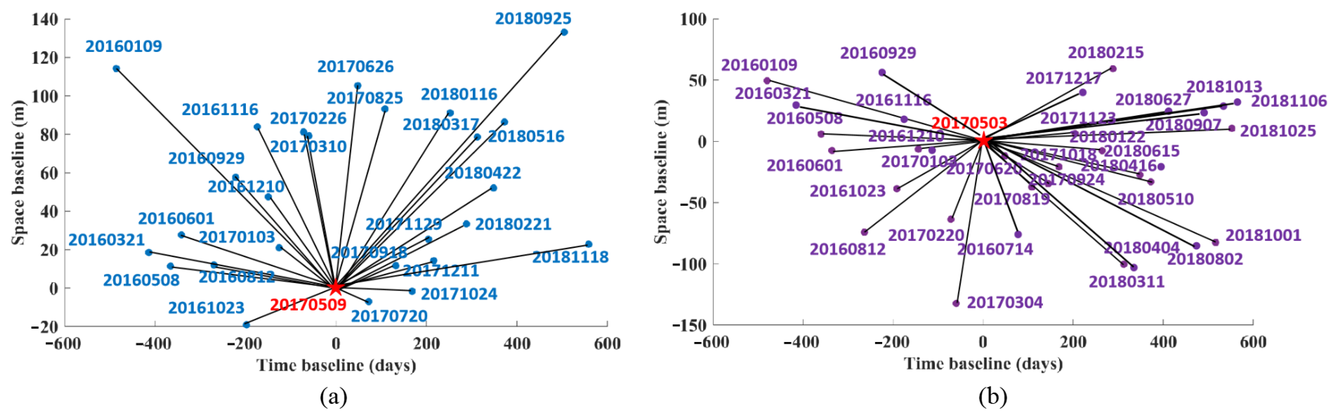
| Track | Time Span | Number | Incidence Angle | HEADING |
|---|---|---|---|---|
| Ascending Track | 20160109–20181118 | 27 | 33.985 | −12.948 |
| Descending Track | 20160109–20181106 | 34 | 39.271 | −170.105 |
Publisher’s Note: MDPI stays neutral with regard to jurisdictional claims in published maps and institutional affiliations. |
© 2022 by the authors. Licensee MDPI, Basel, Switzerland. This article is an open access article distributed under the terms and conditions of the Creative Commons Attribution (CC BY) license (https://creativecommons.org/licenses/by/4.0/).
Share and Cite
Ji, P.; Lv, X.; Wang, R. Deriving 3-D Surface Deformation Time Series with Strain Model and Kalman Filter from GNSS and InSAR Data. Remote Sens. 2022, 14, 2816. https://doi.org/10.3390/rs14122816
Ji P, Lv X, Wang R. Deriving 3-D Surface Deformation Time Series with Strain Model and Kalman Filter from GNSS and InSAR Data. Remote Sensing. 2022; 14(12):2816. https://doi.org/10.3390/rs14122816
Chicago/Turabian StyleJi, Panfeng, Xiaolei Lv, and Rui Wang. 2022. "Deriving 3-D Surface Deformation Time Series with Strain Model and Kalman Filter from GNSS and InSAR Data" Remote Sensing 14, no. 12: 2816. https://doi.org/10.3390/rs14122816
APA StyleJi, P., Lv, X., & Wang, R. (2022). Deriving 3-D Surface Deformation Time Series with Strain Model and Kalman Filter from GNSS and InSAR Data. Remote Sensing, 14(12), 2816. https://doi.org/10.3390/rs14122816