Earth Gravity In-Orbit Sensing: MPC Formation Control Based on a Novel Constellation Model

Abstract

Missions finalized at measuring the space-time variations of the Earth gravity field have become of high relevance in recent years. These missions are indeed of interest for scientific purposes and applications in several fields. Precise observations of the Earth gravity field can be accomplished by measuring the distance between two satellites flying in suitable orbits. Several mission concepts foresee an active formation control to maintain the distance variations between the two satellites within given bounds. In this paper, we first present an original constellation model, called the Triangle Dynamics (TD) model, which is particularly suitable to describe the orbital dynamics of satellite pairs. Open-loop simulations are performed, where the TD model is compared with a standard model, derived from the well-known Hill–Clohessy–Wiltshire (HCW) equations. The simulation results show that the TD model provides more accurate predictions than the HCW model. Then, we propose a formation control approach based on a new Model Predictive Control (MPC) algorithm. The core of this algorithm is the TD model, which is used in real-time to predict the behavior of the satellite pair, allowing the computation of an optimal formation control command. A case study concerned with the Next Generation Gravity Mission (NGGM) is presented to demonstrate the effectiveness of the proposed MPC-TD algorithm.

1. Introduction

In the last few years, in the framework of Earth observation missions, the study of the space-time variations of the Earth’s gravitational field has become an increasingly attractive research topic in industry and academia. Indeed, the gravity anomalies detected during the gravimetric missions allowed mapping with tighter accuracy in terms of the distribution of the terrestrial mass around the planet and its changes in time [1]. The importance of Earth gravity missions is mainly due to the huge relapses that such knowledge can have in several fields of the science, where its applications fall under a wide variety (see, e.g., [2,3]). Indeed, a detailed map of Earth gravity anomalies and its mass distribution offers an important tool for several field of Earth sciences (e.g., oceanography [4], glaciology [5], atmospheric science, meteorology, resources exploitation, and weather and climate studies) and for foreseeing how humans are influencing climate change. For these reasons, over the last decades, space agencies were pushed to design space missions for which their main purpose was to study—from the orbit—the features and behavior of the Earth’s gravitational environment. Examples are missions such as GRACE (Gravity Recovery and Climate Experiment [6]) and GRACE Follow-on [7], launched in 2002 and 2018, respectively, and GOCE (Gravity field and steady state Ocean Circulation Explorer [8]), launched in 2009. After the great scientific success of the aforementioned missions, the European Space Agency (ESA) has proposed several feasibility studies for a Next Generation Gravity Mission (NGGM)—based on the heritage of the previous gravity missions—for which its aim is to measure the temporal variations of the Earth’s gravity field over a full solar cycle [9]. However, in order to perform a more accurate map of the Earth’s gravity anomalies, NGGM will require a higher level of technological standards with respect to its predecessors. Specifically, for what concerns the automatic control side, major challenges will be the satellite-to-satellite tracking technology, based on laser ranging [7], as well as the expected Guidance, Navigation, and Control (GNC) performances and features. Indeed, many Earth observation (or, more specifically, Earth gravimetric) mission concepts usually leverage cooperating satellites to enhance scientific performance [10]. As matter of fact, an enhancement of the quality of data collected from the orbit will require higher performances in terms of constellation formation, attitude, and relative motion control [11,12,13].

Within the GNC framework, Model Predictive Control (MPC) has been accepted as a powerful tool for a wide range of technological applications (see, e.g., [14,15]), which is attractive also for satellite formation control. Indeed, MPC represents a flexible control tool for dealing with linear and nonlinear (in its nonlinear formulation) multivariable systems and is able to cope with both input and state constraints; it can merge into an unique loop with satellite guidance and control tasks. Moreover, the minimization of a performance index also provides the optimal selected system features. Then, it ensures the inherent robustness with respect to external disturbances. MPC is fundamentally based on two key operations: (i) the prediction of the system’s future behavior along a finite time span, which is the so-called prediction horizon; and (ii) the minimization of a suitable cost function in order to obtain an optimal control sequence over the prediction horizon time span. Furthermore, when the receding horizon strategy is adopted, only the first time sample of the optimal control sequence is applied to the plant, while the remainder of the solution is discarded. Then, the same process is iterated for all the successive sampling time steps. Examples of preliminary MPC applications to this class of missions are proposed in [16,17], while the formation flight control scenario is confronted in [18,19,20].

The first contribution of this paper is a new model describing a constellation of two different spacecraft (S/C) traveling in low-Earth orbits. The orbital motion is tailored to space gravimetric missions and is based on the so-called Formation Local Orbital Frame (FLOF) and the triangle virtual structure. Such a formulation, called Triangle Dynamics (TD), allows the derivation of ad hoc differential equations for the description of the spacecraft’s orbit and constellation dynamics. The choice is motivated by the advantage of describing a unique formulation for both the orbit and constellation dynamics [21]. The TD model is compared in simulation with a standard model and is based on the well-known Hill–Clohessy–Wiltshire (HCW) equations. Specifically, the NGGM mission orbits are used as a benchmark for analyzing the difference between the two models in predicting spacecraft behavior over a finite time horizon.

The second contribution of this paper is a novel formation control approach based on a Model Predictive Control (MPC) algorithm. The core of this algorithm is the TD model, which is used in real-time to predict the behavior of the satellite pair, allowing the computation of an optimal formation control command. The MPC choice is motivated by its capability of ensuring a high level of performance in reference tracking, which accounts for command constraints, efficiently limiting command activity and attenuating disturbance effects. Indeed, the purpose of the orbit and formation control is to guarantee formation stability during the long timescales characterizing the mission’s expected lifetime (approximately, an entire solar cycle), while rejecting the external disturbances potentially affecting the inter-satellite distance and driving it outside the prescribed range requirements.

A case study concerned with the NGGM mission is presented to demonstrate the effectiveness of the proposed MPC-TD algorithm. In this case study, simulations are carried out using a detailed nonlinear simulation environment, where the MPC-TD algorithm is compared with a standard MPC approach based on the well-known Hill–Clohessy–Wiltshire (HCW) equations. The simulation results show that the MPC-TD approach can guarantee an effective formation control, outperforming the MPC-HCW approach.

Note that the model proposed in this paper is currently part of the ESA-NASA cooperation in the frame of the MAGIC (Mass Change and Geosciences International Constellation) for future NGGM mission. Indeed the capability of describing, at the same time, the orbit and the constellation dynamics allows the obtainment of a compact and robust model that is suitable for all low-Earth-orbit scientific missions featuring a two-satellite constellation (such as NGGM). Furthermore, when the Global Navigation Satellite System (GNSS) and laser metrology are present, this model can be used for each space scientific mission composed of a formation, even with more stringent requirements in the relative motion between the satellite than only loose formations.

This paper is organized as follows. In Section 2, we present a mathematical model concerning the novel orbit and formation dynamics (Triangle Dynamics, TD). In Section 3, the mathematical formulation of the MPC controller is provided. The TD and HCW orbit and formation models are firstly compared in an open-loop environment in Section 4, while the closed-loop comparison is enclosed in Section 5. Finally, conclusions are drawn in Section 6.

2. Triangle Dynamics Model

This section presents the main aspects of the developed constellation model. Specifically, the orbital dynamics is a special form of the Hill–Clohessy–Wiltshire equations [22,23]. Such formulation, described in detail in [24], is based on the definition of a peculiar formation reference frame (the Formation Local Orbital Frame, FLOF) and the formation triangle virtual structure [21]. These, in turn, lead to the derivation of a novel set of equations describing the spacecraft’s orbit and constellation dynamics. The rationale behind our novel set of CW-type equations is the integration, into an unique model, of the orbit and constellation dynamics through the formation triangle concept [25], defining the so-called Triangle Dynamics (TD) model. In this context, the term “CW-type equations” means equations based on the perturbation of S/C position, in the LVLH frame, with respect to a chief reference frame in the case of a formation of two satellite. Moreover, with stochastic disturbance dynamics, similarly to [26,27], it is possible to account for the orbit’s eccentricity and $J2$ effects, thus making the state equations quasi-periodic.

2.1. Introduction and FLOF Definition

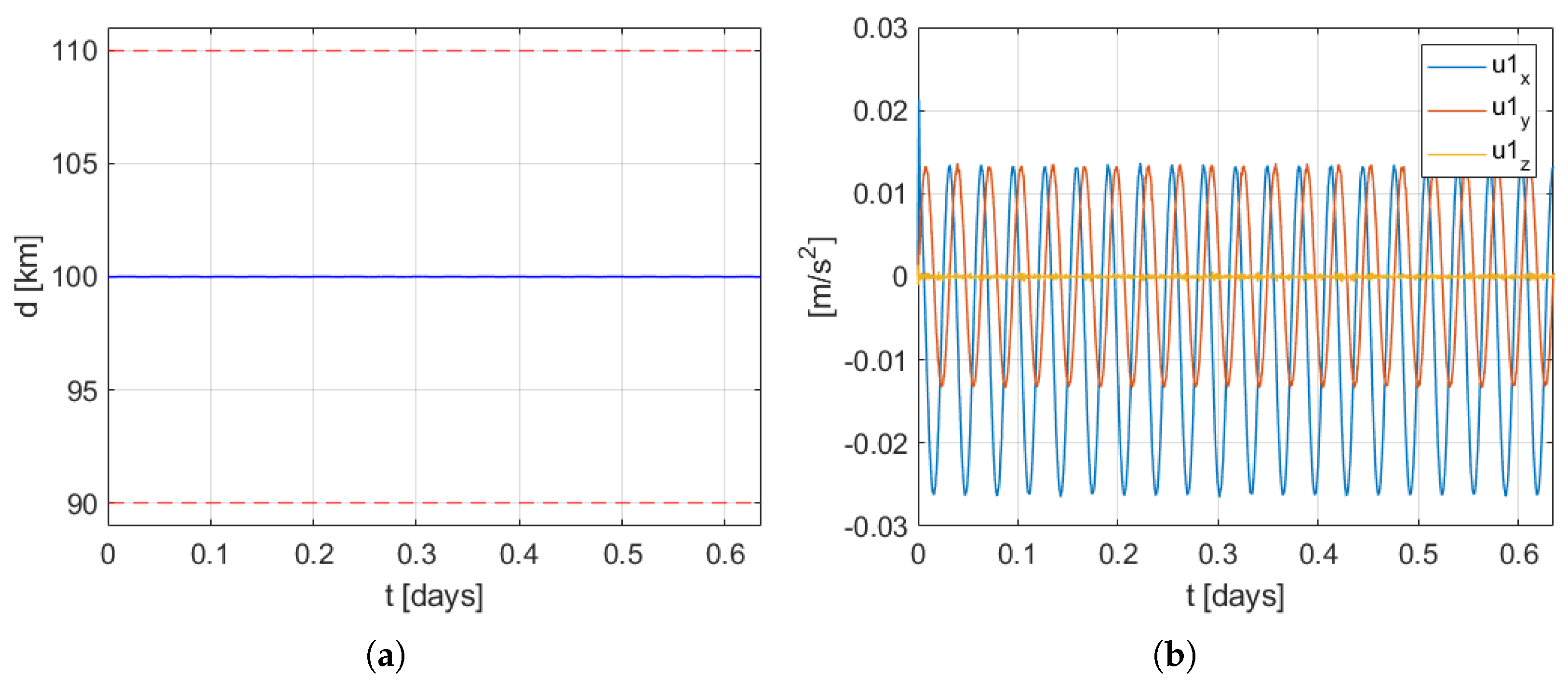
The TD is in charge of describing the orbital altitude of the two spacecraft, as well as their relative distance. From this, we obtain an accurate and robust model that allows the inter-spacecraft or inter-satellite distance d to be easily maintained within a prescribed interval centered at a given nominal value $d_{\mathrm{nom}}$. In this model, the constellation dynamics is derived by the definition of the FLOF reference frame, described in detail below, with the result of achieving the formulation of a special variation of the Hill–Clohessy–Wiltshire (HCW) equations [23], describing the S/C orbit and constellation behavior [25].

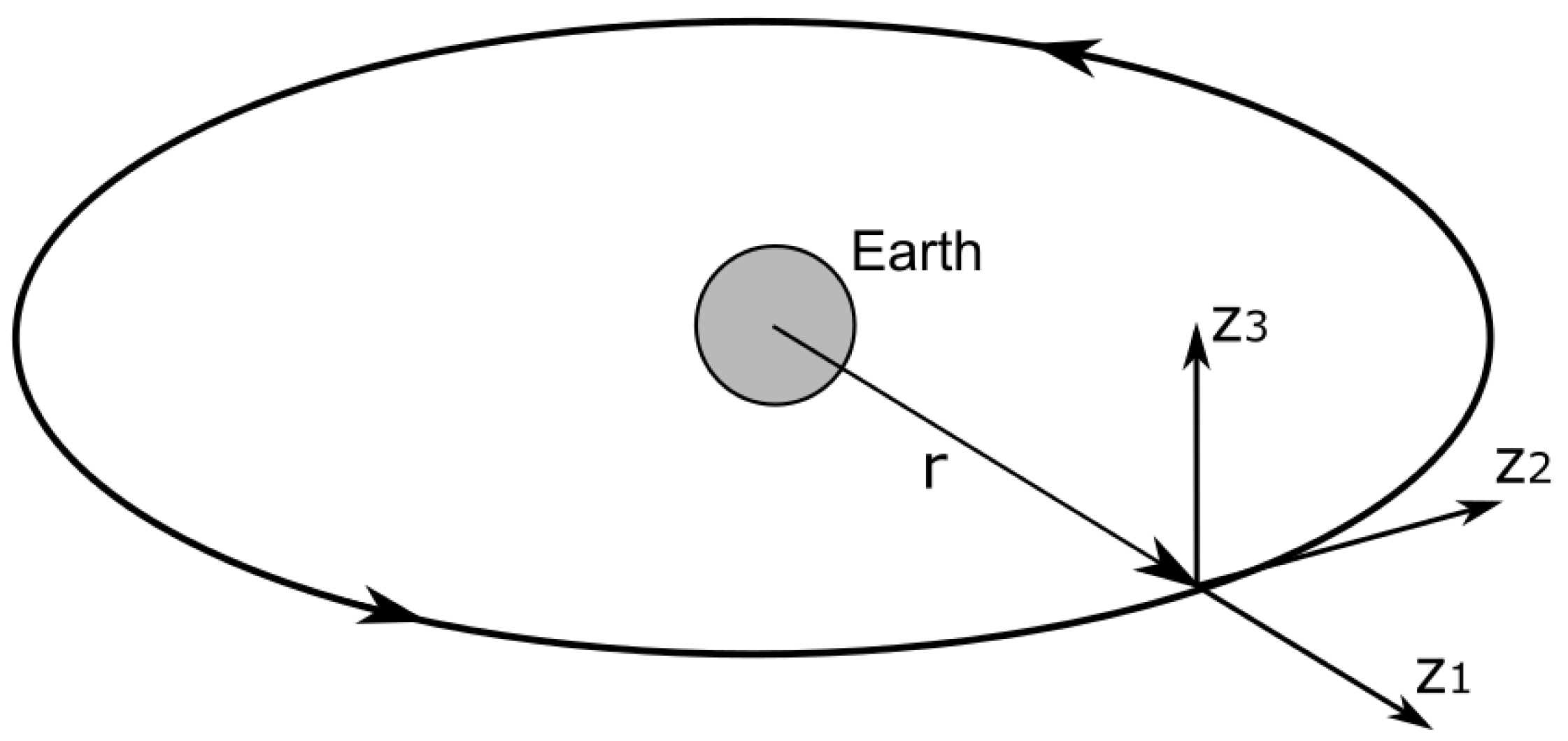
Let us now review the rationale behind the TD model design. As already mentioned, it is based on the definition of a specific orbital reference frame, i.e., the Formation Local Orbital Frame (FLOF) $\mathcal{O}=\{C_F,{\overrightarrow{o}}_1,{\overrightarrow{o}}_2,{\overrightarrow{o}}_3\}$ and the triangle virtual structure, allowing a common description of the constellation altitude and the inter-satellite distance. This triangle is a virtual structure for which its vertices are the two S/C centers of mass (CoMs), $C_1$ and $C_2$ in Figure 1a, in addition to Earth CoM, $C_E$. The FLOF frame is the constellation common reference frame. Hence, the FLOF axes in Equation (1) are defined by the relative satellites position $\Delta \overrightarrow{r}={\overrightarrow{r}}_1-{\overrightarrow{r}}_2$ and by the mean radius $\overrightarrow{r}=({\overrightarrow{r}}_1+{\overrightarrow{r}}_2)/2$, whereas $d=|\Delta \overrightarrow{r}|$ and $r=|\overrightarrow{r}|$. The FLOF frame axes are defined as follows:

$$\begin{array}{c}{\overrightarrow{o}}_1=\frac{\Delta \overrightarrow{r}}{d}\hfill \\ {\overrightarrow{o}}_2=\frac{\overrightarrow{r}/r\times \Delta \overrightarrow{r}/d}{|\overrightarrow{r}/r\times \Delta \overrightarrow{r}/d|}\hfill \\ {\overrightarrow{o}}_3={\overrightarrow{o}}_1\times {\overrightarrow{o}}_2.\hfill \end{array}$$

(1)

Figure 1 shows a sketched representation of the FLOF axes, together with the triangle virtual structure. The first axis ${\overrightarrow{o}}_1$ is referred to as tangential (or along-track), the second one ${\overrightarrow{o}}_2$ is reffered to as lateral (or cross-track), and the third one ${\overrightarrow{o}}_3$ is reffered to as radial. Other than the FLOF and the formation triangle concepts, for the derivation of the TD architecture, common assumptions for Earth gravity sensing missions (such as GOCE) are taken into account. The satellite nominal orbits are assumed to be polar, with an altitude between 300 and $400\mathrm{k}\mathrm{m}$, with the same right ascension of the ascending nodes (in-line constellation). In addition, the satellite-to-satellite distance variations are measured along the satellite-to-satellite line (SSL). SSL is defined as the line connecting the center of mass of the two satellites, and the first FLOF axis ${\overrightarrow{o}}_1$ sets its direction. In a low-Earth-orbit, SSL can be materialized by a differential Global Navigation Satellite System (GNSS).

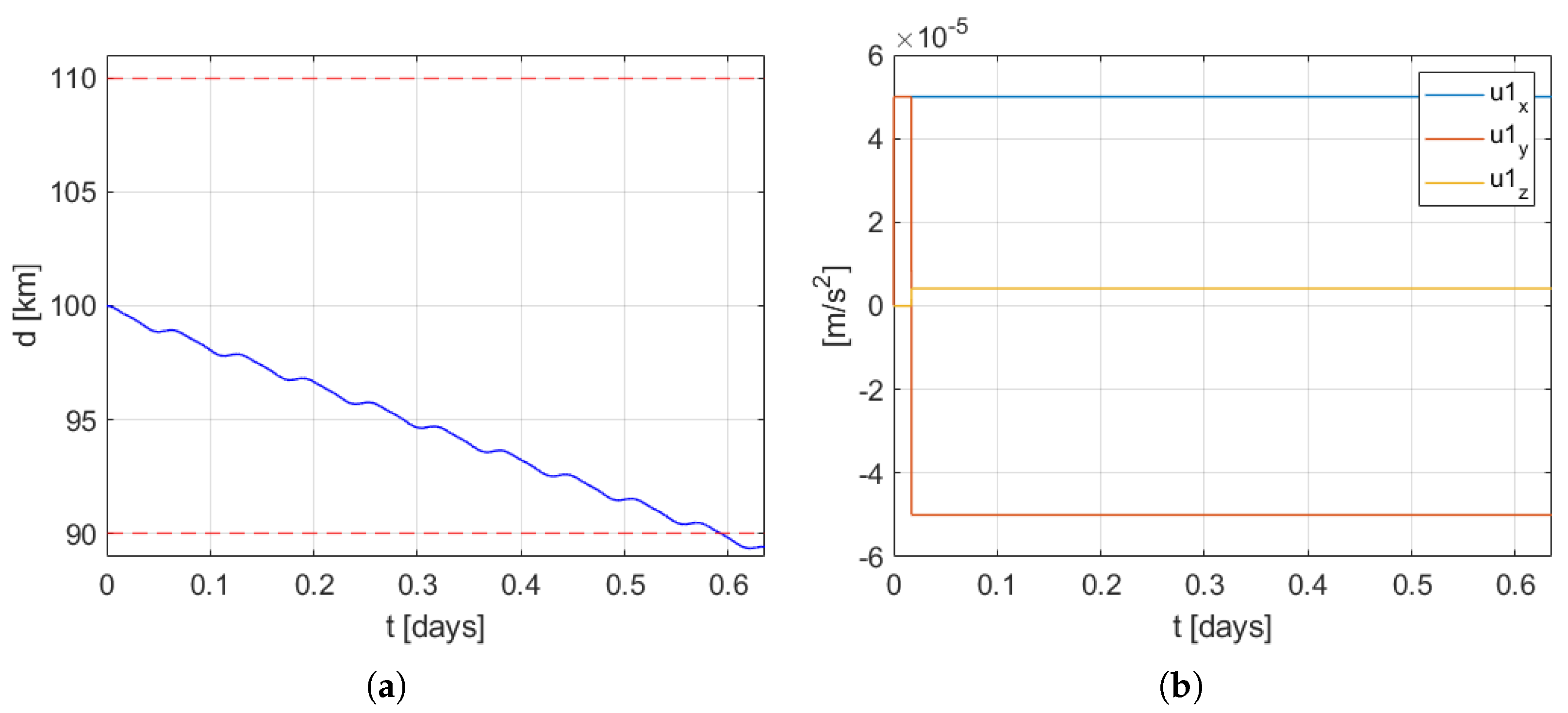
Further assumptions concern the additional control unit tasks. Indeed, both the drag-free control and the attitude and pointing controls are properly working. As a matter of fact, the TD model assumes that the high-frequency ($f>f_{nom}=1/P_{nom}$) forcing accelerations are only due to gravity periodic components that are related to the scientific objective of the gravimetric mission. This can be considered true if the short-term non-gravitational accelerations are canceled by an appropriate control action. In other words, if it is a drag-free control, both linear and angular settings are available. Note that, despite these assumptions (reasonable in this context), the model remains valid even under different conditions than those defined above (as proved in Section 4.2).

2.2. Constellation Dynamics

Before detailing the TD model derivation, a brief account of spacecraft and constellation dynamics is provided. The model should be built with respect to the chief frame of reference, namely the FLOF frame defined in Equation (1). Indeed, the orbit and constellation model requires the preliminary definitions of the orbit and constellation perturbations, which are needed for the definition of triangle dynamics. Let us start by considering the standard satellite CoM inertial dynamics with a GNSS range and rate measurements, ${\mathrm{y}}_{rk}$ and ${\mathrm{y}}_{vk}$, and accelerometer measurements ${\mathrm{y}}_{ak}$:

$$\begin{array}{cc}\hfill {\ddot{\mathrm{r}}}_k\left(t\right)& =-\mathrm{g}\left({\mathrm{r}}_k\left(t\right)\right)+{\mathrm{a}}_k\left(t\right),{\mathrm{r}}_k\left(0\right)={\mathrm{r}}_{k0},{\dot{\mathrm{r}}}_k\left(0\right)={\mathrm{v}}_{k0}\hfill \\ \hfill {\mathrm{y}}_{rk}\left(t\right)& ={\mathrm{r}}_k\left(t\right)+{\mathrm{e}}_{rk}\left(t\right)\hfill \\ \hfill {\mathrm{y}}_{vk}\left(t\right)& ={\dot{\mathrm{r}}}_k\left(t\right)+{\mathrm{e}}_{vk}\left(t\right)\hfill \\ \hfill {\mathrm{y}}_{ak}\left(t\right)& ={\mathrm{P}}_a({\mathrm{a}}_k\left(t\right)+{\mathrm{n}}_{ak}\left(t\right))+{\mathrm{w}}_{ak}\left(t\right),\hfill \end{array}$$

(2)

where $k=1,2$ is the satellite number, and ${\mathrm{e}}_{rk}$ and ${\mathrm{e}}_{vk}$ are the model errors, thus including measurement errors and the effect of neglected dynamics. On the other hand, ${\mathrm{n}}_{ak}$ and ${\mathrm{w}}_{ak}$ are, respectively, the low-frequency and high-frequency accelerometer errors, while ${\mathrm{P}}_a$ denotes accelerometer dynamics. In (2), we define ${\mathrm{a}}_k=({\mathrm{u}}_k+{\mathrm{d}}_k)/m$ that accounts for the non-gravitational accelerations acting upon the k-th S/C, where ${\mathrm{d}}_k$ and ${\mathrm{u}}_k$ are the disturbance and thruster command forces, respectively. Furthermore, m is the spacecraft mass, while $U\left(\mathrm{r}\right)$ is the gravity tensor to be measured in order to retrieve the scientific gravimetry signal, namely the object of an Earth-gravity monitoring mission. The dynamics in Equation (2) is equivalent to the constellation mean and differential dynamics (r and $\Delta \mathrm{r}$), which involves, starting from (2) for each S/C, dropping subscript k and holding the following.

$$\begin{array}{cc}\hfill \ddot{\mathrm{r}}\left(t\right)& =-\frac{\mathrm{g}\left({\mathrm{r}}_1\right)+\mathrm{g}\left({\mathrm{r}}_2\right)}{2}+\mathrm{a}\left(t\right)\hfill \\ \hfill & =-\mathrm{g}\left(\mathrm{r}\right)+\mathrm{a}\left(t\right),\mathrm{r}\left(0\right)={\mathrm{r}}_0,\dot{\mathrm{r}}\left(0\right)={\mathrm{v}}_0\hfill \\ \hfill \Delta \ddot{\mathrm{r}}\left(t\right)& =-(\mathrm{g}\left({\mathrm{r}}_1\right)-\mathrm{g}\left({\mathrm{r}}_2\right))+\Delta \mathrm{a}\left(t\right)\hfill \\ \hfill & =-U\left(\mathrm{r}\right)\Delta \mathrm{r}\left(t\right)+\Delta \mathrm{a}\left(t\right),\Delta \mathrm{r}\left(0\right)=\Delta {\mathrm{r}}_0,\Delta \dot{\mathrm{r}}\left(0\right)=\Delta {\mathrm{v}}_0.\hfill \end{array}$$

(3)

We also define the following.

$$\begin{array}{c}\hfill \mathrm{a}=\frac{{\mathrm{a}}_1+{\mathrm{a}}_2}{2},\Delta \mathrm{a}={\mathrm{a}}_1-{\mathrm{a}}_2.\end{array}$$

(4)

Let us recall that the drag-free setting aims at reaching, in (3), the following conditions.

$$\begin{array}{c}\hfill {\mathrm{a}}_k=0\Rightarrow \mathrm{a}=0,\Delta \mathrm{a}=0.\end{array}$$

(5)

From (5), it follows that the drag-free constellation time-evolution is the free response of the Equation (3). This allows the correlation of the interferometric measurements of $\Delta \mathrm{r}$ with gravity tensor $U\left(\mathrm{r}\right)$ to be measured to retrieve the scientific observable of interest. As a matter of fact, the condition in (5) is achieved by forcing the drag-free command ${\mathrm{u}}_k$ to cancel the real-time prediction of the environment term ${\widehat{\mathrm{d}}}_k$ obtained from accelerometer wide-band measurements. Notwithstanding, this cancellation occurs for less than some residuals mainly due to the limited bandwidth of the drag-free control law, causality, and high-frequency accelerometer errors.

$$\begin{array}{c}\hfill {\mathrm{u}}_k=-{\widehat{\mathrm{d}}}_k\Rightarrow {\mathrm{a}}_k=(-{\mathrm{d}}_k+{\widehat{\mathrm{d}}}_k)/m\cong {\mathrm{w}}_{ak}\ne 0.\end{array}$$

(6)

The effect of such residuals, as stated before, would impinge on the constellation’s (and attitude’s) stability, without the proper position/velocity feedback ensured by a formation control.

Generally speaking, the constellation and orbit perturbations, needed to build the constellation model, can be expressed in two ways: (i) the standard Hill–Clohessy–Wiltshire perturbations [23], defined as the 3D S/C CoM displacement $\delta {\mathrm{r}}_k={\mathrm{r}}_k-{\mathrm{r}}_{nom,k}$ from a Keplerian reference orbit ${\mathrm{r}}_{nom,k}\left(t\right)$ that is either circular or elliptical [27] or (ii) the S/C radial and angular perturbations approach, which is adopted in this study. Specifically, the radial and angular perturbations consist in the following: (i) the radial perturbation $\delta {\mathrm{r}}_k{\mathrm{l}}_{3,k}=({\mathrm{r}}_k-{\mathrm{r}}_{nom,k}){\mathrm{l}}_{3,k}$, ${\mathrm{l}}_{3,k}$ being the local-vertical-local-horizontal (LVLH) radial axis, and (ii) the angular rate ${\omega }_k$ of the actual orbit LVLH frame. It can be proven that ${\omega }_{xk}=0$, ${\omega }_k$ has only two degrees-of-freedom, adding up to the radial perturbation $\delta {\mathrm{r}}_k{\mathrm{l}}_{3,k}$ to a total of three degrees of freedom (DoFs) for the Cartesian perturbations. As a matter of fact, a specific combination of Cartesian and angular perturbations can be extended to a two-satellite constellation with the help of the FLOF frame, defined in Equation (1). As sketched in Figure 1b, a nominal reference sphere of radius $r_{nom}$ (i.e., the nominal constellation altitude) can be associated to the constellation CoM r, defining the nominal orbit, while a nominal constellation SSL, with a length of $d_{nom}$ (i.e., the mean reference inter-satellite distance) and tangent to the reference sphere, can be associated to the relative position $\Delta \mathrm{r}$. Indeed, the constellation radius r and the satellite radii (${\mathrm{r}}_1$ and ${\mathrm{r}}_2$) hold the following:

$$\begin{array}{cc}\hfill \mathrm{r}& =r_x{\overrightarrow{o}}_1+r_z{\overrightarrow{o}}_3,{\mathrm{r}}_1-{\mathrm{r}}_2=d_{nom}{\overrightarrow{o}}_1\hfill \\ \hfill {\mathrm{r}}_1& =\left(r_x+\frac{d}{2}\right){\overrightarrow{o}}_1+r_z{\overrightarrow{o}}_3,{\mathrm{r}}_2=\left(r_x-\frac{d}{2}\right){\overrightarrow{o}}_1+r_z{\overrightarrow{o}}_3,\hfill \end{array}$$

(7)

where the SSL distance is d, and the triangle’s height is $r_z$, which is the component of the constellation radius r along the third FLOF axis ${\overrightarrow{o}}_3$ (see Figure 1). Furthermore, $r_x$ is the mean radius component along the SSL direction ${\overrightarrow{o}}_1$, defining the radius’s orthogonality with respect to the triangle base vector $\Delta \mathrm{r}={\mathrm{r}}_1-{\mathrm{r}}_2$ (see Figure 1). As a matter of fact, $r_x$ is proportional to the satellite radii difference. Indeed, its nominal condition, namely $r_x=0$, is a target of the control action, which tries to align radius r to ${\overrightarrow{o}}_3$, thus making the triangle isosceles. Consequently, three Cartesian perturbations in FLOF coordinates, $\delta d$, $\delta r_x$, and $\delta r_z$, can be defined as follows.

$$\begin{array}{cc}\hfill \Delta \mathrm{r}& =(d_{nom}+\delta d){\overrightarrow{o}}_1\hfill \\ \hfill \mathrm{r}& =r_z{\overrightarrow{o}}_3+r_x{\overrightarrow{o}}_1=(r_{nom}+\delta r_z){\overrightarrow{o}}_3+(0+\delta r_x){\overrightarrow{o}}_1.\hfill \end{array}$$

(8)

The perturbations defined in Equation (8) will be directly leveraged to build the TD model based on the FLOF frame. Specifically, perturbation $\delta r_x$ is referred to as ‘differential altitude’ or ‘differential radius’. Indeed, from Figure 1b, it is possible to observe that $\delta r_x$ is proportional to the mean radius difference of the satellite orbits. In addition, three DoFs are provided by the 3D nonzero components of the FLOF angular rate vector $\omega$. Therefore, we have a total of six DoFs describing the constellation dynamics.

It is worth point out that the three perturbations in (8), being defined with respect to a reference sphere of radius $r_{nom}$, perfectly fit the in-line constellation type and is characterized by a circular reference orbit.

2.3. TD Model Derivation

In this section, the derivation of the continuous-time constellation dynamics model, namely the Triangle Dynamics model, is considered. Specifically, in the following, a brief development from the triangle differential dynamics to the continuous-time final models is provided. Of course, the model developed here is defined with respect to the FLOF frame (see Equation (1)).

The constellation dynamics expresses the triangle dynamics based on the differential equations of the six DoFs defined above in Section 2.1: (i) the three Cartesian perturbations, namely the distance, the differential and mean altitudes ($\delta d,\delta r_x,\delta r_z$) defined in Equation (8), and (ii) the three FLOF angular rate perturbations defined by $\omega ={\omega }_{nom}+\delta \omega$.

$$\begin{array}{c}\hfill \omega ={\omega }_x{\overrightarrow{o}}_1+{\omega }_y{\overrightarrow{o}}_2+{\omega }_z{\overrightarrow{o}}_3.\end{array}$$

(9)

Hence, by starting from the relative satellite position vector $\Delta \mathrm{r}=d{\overrightarrow{o}}_1$ in (8), which is aligned to the FLOF axis ${\overrightarrow{o}}_1$ by construction, as sketched in Figure 1, it is possible to derive the differential equation of the inter-satellite distance variable, d. Let us observe that, since $\Delta \mathrm{r}$ has three DoFs, we obtain three scalar second-order differential equations: (i) One expressing the second-derivative of the distance, namely the distance variation acceleration $\ddot{d}$, while two further differential equations detail the pitch and yaw angular accelerations of ${\overrightarrow{o}}_1$, namely (ii) ${\dot{\omega }}_y$ and (iii) ${\dot{\omega }}_z$. As a result, the differential radius $\Delta \mathrm{r}$ kinematic equation in FLOF coordinates reads as follows:

$$\begin{array}{c}\Delta \ddot{\mathrm{r}}=\left(\ddot{d}-d({\omega }_y^2+{\omega }_z^2)\right){\overrightarrow{o}}_1\hfill \\ +\left(2\dot{d}{\omega }_z+d({\dot{\omega }}_z+{\omega }_x{\omega }_y)\right){\overrightarrow{o}}_2\hfill \\ +\left(-2\dot{d}{\omega }_y+d(-{\dot{\omega }}_y+{\omega }_x{\omega }_z)\right){\overrightarrow{o}}_3,\hfill \end{array}$$

(10)

where $\omega$ is the FLOF angular rate, while $\dot{\omega }$ is the angular acceleration. Consequently, by wisely comparing components with respect to the differential radius kinematics in Equation (10) with the differential dynamic equation in (3) (second line), we have the following:

$$\begin{array}{cc}\hfill \ddot{d}& =-d({\omega }_y^2+{\omega }_z^2)-\Delta g_x+\Delta a_x\hfill \\ \hfill d{\dot{\omega }}_z& =-2\dot{d}{\omega }_z-d{\omega }_x{\omega }_y-\Delta g_y+\Delta a_y\hfill \\ \hfill d{\dot{\omega }}_y& =-2\dot{d}{\omega }_y+d{\omega }_x{\omega }_z-\Delta g_z+\Delta a_z,\hfill \end{array}$$

(11)

which describes the FLOF dynamics of the first three DoFs (d, ${\omega }_y$, and ${\omega }_z$) out of the six needed to build the complete triangle model (Figure 1b). In (11), the FLOF coordinates of the differential external acceleration $\Delta \mathrm{a}$ in (4) are highlighted. Moreover, the gravity gradient term $\Delta \mathrm{g}=\mathrm{g}\left({\mathrm{r}}_1\right)-\mathrm{g}\left({\mathrm{r}}_2\right)$ can be expressed in FLOF coordinates and through the identified triangle variables (r and $\Delta \mathrm{r}$) in terms of the spherical gravity terms only, while ideally arranging the higher-order terms in the external acceleration contribution $\Delta \mathrm{a}$:

$$\begin{array}{cc}\hfill \Delta \mathrm{g}(\mathrm{r},\Delta \mathrm{r})& =\Delta g_x{\overrightarrow{o}}_1+\Delta g_y{\overrightarrow{o}}_2+\Delta g_z{\overrightarrow{o}}_3\hfill \\ \hfill & =-\left(\Delta G{r}_x+G\frac{d}{2}\right){\overrightarrow{o}}_1-\Delta G{r}_z{\overrightarrow{o}}_3,\hfill \end{array}$$

(12)

where $\Delta G=\mu (r_2^3-r_1^3)/r_2^3{r}_1^3$ and $G=\mu (r_2^3+r_1^3)/r_2^3{r}_1^3$. For the sake of completeness, in this context, with spherical gravity, a gravity model defined by a central potential (spherical symmetry) is intended, defined as $U=-\mu /r$, where $\mu$ is Earth’s gravitational parameter and r is the distance from Earth’s CoM to the orbiting spacecraft’s CoM. Moreover, we can say that the model simplification in (12) could impinge on the model capability’s in describing the constellation dynamic behavior only in case that distance d is not a negligible fraction of the mean constellation radius $r=\left|\mathrm{r}\right|$. Indeed, in that case, where the dimensional coefficient $\alpha =d_{nom}/r_{nom}$, which will be introduced later (see (18)), is greater than, let us say, $0.01$, the $J2$ gravity term (i.e., the second order harmonics of the gravity gradient expansion) contribution to the gravity gradient should be accounted for to ensure a more reliable control action. Thus, from (11) and (12), the following holds:

$$\begin{array}{cc}\hfill \ddot{d}& =-{\omega }_s^2\left(r\right)d\left(1-3\frac{r_x^2}{r^2}\right)+d\left({\omega }_y^2+{\omega }_z^2\right)+\Delta a_x\hfill \\ \hfill {\dot{\omega }}_z& =-2\dot{d}\frac{{\omega }_z}{d}-{\omega }_y{\omega }_x+\frac{\Delta a_y}{d}\hfill \\ \hfill {\dot{\omega }}_y& =-3{\omega }_0^2\left(r\right)\frac{r_x{r}_z}{r^2}-\frac{2}{d}\dot{d}{\omega }_y+{\omega }_z{\omega }_x-\frac{\Delta a_z}{d},\hfill \end{array}$$

(13)

where $r=\left|\mathrm{r}\right|$, ${\omega }_s^2=\mu /r^3$ is the mean orbital rate, while $r_x$ and $r_z$ come from the definitions in (8).

As a further step, let us detail the second set of equations completing the six constellation degrees of freedom. For this purpose, let us focus on the mean and the differential altitude, $r_z$ and $r_x$, by computing the kinematic equation of the constellation mean radius r and then applying the same component-wise comparison procedure between the computed radial kinematics (14) and the mean dynamic equation in (3) (first line). Thus, if the following constellation radial kinematics holds:

$$\begin{array}{c}\ddot{\mathrm{r}}=\left({\ddot{r}}_x+{\dot{\omega }}_y{r}_z+2{\omega }_y{\dot{r}}_z-\left({\omega }_y^2+{\omega }_z^2\right)r_x+{\omega }_x{\omega }_z{r}_z\right){\overrightarrow{o}}_1\hfill \\ +\left(-{\dot{\omega }}_x{r}_z+{\dot{\omega }}_z{r}_x+{\omega }_x{\omega }_y{r}_x+{\omega }_y{\omega }_z{r}_z+2\left(-{\omega }_x{\dot{r}}_z+{\omega }_z{\dot{r}}_x\right)\right){\overrightarrow{o}}_2\hfill \\ +\left({\ddot{r}}_z-{\dot{\omega }}_y{r}_x-2{\omega }_y{\dot{r}}_x-\left({\omega }_x^2+{\omega }_y^2\right)r_z+{\omega }_x{\omega }_z{r}_x\right){\overrightarrow{o}}_3,\hfill \end{array}$$

(14)

from (14) and (3), the radial dynamics in FLOF coordinates read as follows.

$$\begin{array}{cc}\hfill {\ddot{r}}_x& =-{\dot{\omega }}_y{r}_z-2{\omega }_y{\dot{r}}_z+\left({\omega }_y^2+{\omega }_z^2\right)r_x-{\omega }_x{\omega }_z{r}_z-g_x+a_x\hfill \\ \hfill {\dot{\omega }}_x{r}_z& ={\dot{\omega }}_z{r}_x+{\omega }_x{\omega }_y{r}_x+{\omega }_y{\omega }_z{r}_z+2\left(-{\omega }_x{\dot{r}}_z+{\omega }_z{\dot{r}}_x\right)+g_y-a_y\hfill \\ \hfill {\ddot{r}}_z& ={\dot{\omega }}_y{r}_x+2{\omega }_y{\dot{r}}_x+\left({\omega }_x^2+{\omega }_y^2\right)r_z-{\omega }_x{\omega }_z{r}_x-g_z+a_z.\hfill \end{array}$$

(15)

Equation (15) describes the FLOF dynamics of the further three DoFs ($r_x$, ${\omega }_x$, and $r_z$) needed to build the complete triangle model (Figure 1b). In (15), the mean gravity term, $\mathrm{g}(\mathrm{r},\Delta \mathrm{r})=\left(\mathrm{g}\left({\mathrm{r}}_1\right)+\mathrm{g}\left({\mathrm{r}}_2\right)\right)/2=g_x{\overrightarrow{o}}_1+g_y{\overrightarrow{o}}_2+g_z{\overrightarrow{o}}_3$ in FLOF coordinates, is still described through the identified constellation triangle variables (r and $\Delta \mathrm{r}$) in terms of the spherical gravity terms only, as specified above. Indeed, the higher-order terms are again ideally accounted for in the three components of the external mean acceleration contribution a from (4). As a result, the second set of differential equations, concerning the triangle DoFs $r_x$, $r_z$ (Figure 1b), and ${\omega }_x$, reads as follows:

$$\begin{array}{cc}\hfill {\ddot{r}}_x& =-{\omega }_s^2\left(r\right)r_x\left(1-3\frac{r_z^2}{r^2}\right)-2{\omega }_y{\dot{r}}_z+\left({\omega }_y^2+{\omega }_z^2\right)r_x\hfill \\ & -2{\omega }_z{\omega }_x{r}_z+2\frac{r_z}{d}{\omega }_y\dot{d}+\frac{r_z}{d}\Delta a_z+a_x\hfill \\ \hfill {\ddot{r}}_z& =-{\omega }_s^2\left(r\right)r_z\left(1+3\frac{r_x^2}{r^2}\right)+2{\omega }_y{\dot{r}}_x+\left({\omega }_x^2+{\omega }_y^2\right)r_z\hfill \\ & -2\frac{r_x}{d}{\omega }_y\dot{d}-\frac{r_x}{d}\Delta a_z+a_z\hfill \\ \hfill {\dot{\omega }}_x& =\frac{2}{r_z}\left(-{\omega }_x{\dot{r}}_z+{\omega }_z{\dot{r}}_x\right)+{\omega }_z{\omega }_y-2\frac{r_x}{d{r}_z}{\omega }_z\dot{d}+\frac{r_x}{d{r}_z}\Delta a_y-\frac{a_y}{r_z},\hfill \end{array}$$

(16)

where ${\omega }_s$ is defined above.

Provided with the two equation sets from (13) and (16) that fully describe two-spacecraft constellation dynamics by means of triangle dynamics and the perturbation variables from (8), we proceed by adopting the perturbation equations modeling strategy. Indeed, since the control is expected to keep the selected constellation variables close to their nominal value, some equilibrium points and trajectories can be defined for the control design purpose. Hence, we seek the equilibrium by setting the constellation variable derivatives in (13) and (16) to zero under zero input signals, thus finding the following equilibrium components and making up the equilibrium state vector ${\mathrm{x}}_{eq}$.

$$\begin{array}{cc}\hfill d_{eq}& =d_{nom},r_{z,eq}=r_{nom},r_{x,eq}=0\hfill \\ \hfill {\omega }_{y,eq}& ={\omega }_s\left(r_{nom}\right)={\omega }_{nom},{\omega }_{x,eq}={\omega }_{z,eq}=0.\hfill \end{array}$$

(17)

Accordingly, by means of (17), we can define the triangle perturbed state variables, namely $\delta \mathrm{x}=\mathrm{x}-{\mathrm{x}}_{eq}$, as well as the external non-gravitational acceleration input vector ${\mathrm{a}}_f$:

$$\begin{array}{c}\hfill \begin{array}{c}\hfill \delta {\mathrm{x}}_f=\left[\begin{array}{c}\delta d=d-d_{nom}\\ {\rho }_x=-\alpha r_x\\ \delta {\rho }_z=\alpha (r_z-r_{nom})\end{array}\right],\delta {\mathrm{v}}_f=\left[\begin{array}{c}\delta \dot{d}/{\omega }_{nom}\\ {\dot{\rho }}_x/{\omega }_{nom}\\ \delta {\dot{\rho }}_z/{\omega }_{nom}\\ w_x=d_{nom}{\omega }_x/{\omega }_{nom}\\ w_y=d_{nom}({\omega }_y-{\omega }_{nom})/{\omega }_{nom}\\ w_z=d_{nom}{\omega }_z/{\omega }_{nom}\end{array}\right],{\mathrm{a}}_f=\left[\begin{array}{c}\Delta a_x\\ \Delta a_y\\ \Delta a_z\\ \alpha a_x\\ \alpha a_y\\ \alpha a_z\end{array}\right],\end{array}\end{array}$$

(18)

where the perturbed state vector $\delta \mathrm{x}$ is split into its sub-vectors $\delta {\mathrm{x}}_f$ and $\delta {\mathrm{v}}_f$, accounting for the length and the rate state variables all in length unit, whereas the adimensional scale factor $\alpha =d_{nom}/r_{nom}$ is defined as above. Hence, the orbit and constellation dynamics is based on the perturbation differential equations, for which its equations were built by combining the kinematics equations involving the six selected perturbations with the triangle dynamics, as explained above. The final perturbation equations were used for the control design after having been linearised around the equilibrium point defined in (17). As a result, by rewriting model Equations (13) and (16) in the equilibrium conditions through the perturbed state variables and inputs (18), the following linear time-invariant (LTI) continuous-time state equations hold follows:

$$\begin{array}{cc}\hfill \left[\begin{array}{c}\delta {\dot{\mathrm{x}}}_f\\ \delta {\dot{\mathrm{v}}}_f\end{array}\right]\left(t\right)& ={\omega }_{nom}\left[\begin{array}{cc}0& A_{12}\\ A_{21}& A_{22}\end{array}\right]\left[\begin{array}{c}\delta {\mathrm{x}}_f\\ \delta {\mathrm{v}}_f\end{array}\right]\left(t\right)+\frac{1}{{\omega }_{nom}}\left[\begin{array}{c}0\\ B_2\end{array}\right]{\mathrm{a}}_f\left(t\right)\hfill \\ \hfill {\mathrm{y}}_f\left(t\right)& =\left[\begin{array}{cc}{C}_1& C_2\end{array}\right]\left[\begin{array}{c}\delta {\mathrm{x}}_f\\ \delta {\mathrm{v}}_f\end{array}\right]\left(t\right),\hfill \end{array}$$

(19)

for which matrices $A_{12}$, $A_{21}$, $A_{22}$, and $B_2$ are parameter free. As a design choice, the angular rate components, ${\omega }_x$, ${\omega }_y$, and ${\omega }_z$, are normalized in (19), through the definition of the state variables $w_x$ (roll), $w_y$, (pitch), and $w_z$ (yaw) in (18). By doing so, all the state variables in $\delta \mathrm{x}$ are length increments, with the same unit of measurements, i.e., the meter, and the constellation model looks more homogeneous and is easier to interface with the model’s inputs and outputs. Furthermore, from (19), we can observe how the roll and yaw state variables, $w_x$ and $w_z$, are decoupled from the other state variables. Likewise, decoupling applies also to input signals $\Delta a_y$ and $\alpha a_y$, which are orthogonal to the formation plane. The state matrix of the model (19) is of ninth order, and the nine eigenvalues are as follows.

$$\begin{array}{c}\hfill {\lambda }_{1,2,3}=0,{\lambda }_{4,5,6}=j{\omega }_{nom},{\lambda }_{7,8,9}=-j{\omega }_{nom}.\end{array}$$

(20)

Hence, the three eigenvalues ${\lambda }_{1,2,3}=0$ need to be stabilized, while the other ones are imposed by the nature. As a matter of fact, by including also the angular kinematics of the triangle, further zero eigenvalues would arise. On the other hand, the out-of-plane constellation dynamics, encompassing the (normalized) roll and yaw angular rates, $w_x$ and $w_z$, are decoupled in (19) and likewise its input signals $\Delta a_y$ and $\alpha a_y$, and it will be neglected from here. Thus, from the completed model in (19), let us consider only the three Cartesian perturbations, namely the differential height ${\rho }_x$, the mean height ${\rho }_z$, and the distance $\delta d$ in $\delta {\mathrm{x}}_f$ and their normalized rates, in $\delta {\mathrm{v}}_f$, in addition to the normalized perturbation of orbital rate $w_y$. Moreover, the input vector is restricted to the four in-plane input variables in ${\mathrm{a}}_f$. It is worth noting that the restricted seventh-order model from (19) can be proven to be observable and controllable when assuming ${\mathrm{y}}_f\left(t\right)=\delta {\mathrm{x}}_f\left(t\right)$, which implies $C_1=I_3$ and $C_2=0$. Hence, after some treatment, we have the following:

$$\begin{array}{cc}\hfill & \left[\begin{array}{c}\dot{\mathrm{r}}\\ \dot{\mathrm{w}}\end{array}\right]\left(t\right)=\left[\begin{array}{cc}0& A_{12}\\ A_{21}& A_{22}\end{array}\right]\left[\begin{array}{c}\mathrm{r}\\ \mathrm{w}\end{array}\right]\left(t\right)+\left[\begin{array}{c}0\\ B_2\end{array}\right]\mathrm{u}\left(t\right)\hfill \\ \hfill & {\mathrm{y}}_f\left(t\right)=\left[\begin{array}{cc}I& 0\end{array}\right]\left[\begin{array}{c}\mathrm{r}\\ \mathrm{w}\end{array}\right]\left(t\right),\left[\begin{array}{c}\mathrm{r}\\ \mathrm{w}\end{array}\right]\left(0\right)=\left[\begin{array}{c}{\mathrm{r}}_0\\ {\mathrm{w}}_0\end{array}\right]\hfill \\ \hfill & \mathrm{r}=\left[\begin{array}{c}{\rho }_x=\alpha \delta r_x\\ {\rho }_z=\alpha \delta r_z\\ \delta d\end{array}\right],\mathrm{w}=\left[\begin{array}{c}{w}_x\\ w_z\\ w_d\\ w_y\end{array}\right],\mathrm{u}=\left[\begin{array}{c}{u}_{fx}\\ u_{fz}\\ \Delta u_{fx}\\ \Delta u_{fz}\end{array}\right],\hfill \end{array}$$

(21)

where the following is the case.

$$\begin{array}{cc}\hfill A_{12}& ={\omega }_{nom}\left[\begin{array}{cccc}1& 0& 0& 0\\ 0& 1& 0& 0\\ 0& 0& 1& 0\end{array}\right],A_{21}=3{\omega }_{nom}\left[\begin{array}{ccc}1& 0& 0\\ 0& 1& 0\\ 0& 1& 0\\ -1& 0& 0\end{array}\right]\hfill \\ \hfill A_{22}& =2{\omega }_{nom}\left[\begin{array}{cccc}0& -1& 1& 0\\ 1& 0& 0& 1\\ 0& 0& 0& 1\\ 0& 0& -1& 0\end{array}\right],B_2=\left[\begin{array}{cccc}\alpha & 0& 0& 1\\ 0& \alpha & 0& 0\\ 0& 0& 1& 0\\ 0& 0& 0& -1\end{array}\right]/{\omega }_{nom}.\hfill \end{array}$$

(22)

The eigenvalues of the system are as follows.

$${\lambda }_{1,2,3}=0,{\lambda }_{4,5,6,7}=\pm j{\omega }_{nom}.$$

(23)

From the derived LTI model, it follows that only seven states are required to control a formation of two S/C. This can be a benefit from a control design point of view with respect to the use of the HCW model. Indeed, with the HCW equations, six states are used to provide the approximate dynamics of a single spacecraft with respect to an orbiting frame. This results in the implementation of two different HCW models and then in the use of twelve states for controlling a formation of two satellites.

3. Model Predictive Control

Since, as described in Section 2.3, the triangle dynamics model is linear time-invariant, a model predictive control algorithm can be employed. Consider the general form of linear continuous-time dynamic systems described by the following state equations:

$$\begin{array}{cc}\hfill & \dot{x}\left(t\right)=Ax\left(t\right)+Bu\left(t\right)\hfill \\ \hfill & y\left(t\right)=Cx\left(t\right)+Du\left(t\right)\hfill \end{array}$$

(24)

where $x\in {\mathbb{R}}^{n_x}$, $u\in {\mathbb{R}}^{n_u}$, and $y\in {\mathbb{R}}^{n_y}$ are the state, the input, and the output, respectively, $A\in {\mathbb{R}}^{n_x\times n_x}$ is the state transition matrix, $B\in {\mathbb{R}}^{n_x\times n_u}$ is the input matrix, $C\in {\mathbb{R}}^{n_y\times n_x}$ is the output matrix, and $D\in {\mathbb{R}}^{n_y\times n_u}$ is the matrix that allows a direct coupling between u and y.

We assume that the state x is measured in real time, with a sampling time $T_S$, according to $x\left(t_k\right)$, $t_k=T_{S}k$, $k=0,1,\dots$. If this assumption does not hold, an observer can be employed. At each time $t=t_k$, a prediction of the system state and output evolution over the finite time interval $[t,t+T_P]$ is performed, where $T_P\ge T_S$ is the prediction horizon. The prediction is obtained by integrating Equation (24). At any time $\tau \in [t,t+T_P]$, the predicted output $\widehat{y}\left(\tau \right)\equiv \widehat{y}(\tau ,x\left(t\right),u(t:\tau ))$ is a function of the ‘initial’ state $x\left(t\right)$ and the input signal $u(t:\tau )$. Notation $u(t:\tau )$ is used to indicate the model’s input signal in interval $[t,\tau ]$.

The idea behind the MPC is to look, at each time $t=t_k$, for an input signal $u^{*}(t:t+T_P)$ such that $\widehat{y}(\tau ,x\left(t\right),u(t:\tau ))$ has the desired behavior in time interval $[t,t+T_p]$ by minimizing a suitable cost function $J\left(u(t:t+T_p)\right)$ subject to possible constraints that may occur during the system’s operations. Mathematically, at each time $t=t_k$, the following optimization problem is solved.

$$\begin{array}{cc}\hfill & u^{*}(t_k:t_k+T_p)=arg\underset{\widehat{u}\left(·\right)}{min}J\left(\widehat{u}(t_k:t_k+T_p)\right)\hfill \\ \hfill & \mathrm{subject}\mathrm{to}:\hfill \\ \hfill & \dot{\widehat{x}}\left(\tau \right)=A\widehat{x}\left(\tau \right)+B\widehat{u}\left(\tau \right),\widehat{x}\left(t_k\right)=x\left(t_k\right)\hfill \\ \hfill & \widehat{y}\left(\tau \right)=C\widehat{x}\left(\tau \right)+D\widehat{u}\left(\tau \right)\hfill \\ \hfill & \widehat{x}\left(\tau \right)\in X_C,\widehat{y}\left(\tau \right)\in Y_C,\widehat{u}\left(\tau \right)\in U_C.\hfill \end{array}$$

(25)

The first two constraints in the optimization problem (25) ensure that the predicted state and output are consistent with the system’s Equation (24), while $X_C$, $Y_C$, and $U_C$ are suitable sets describing possible constraints on the state, output, and input, respectively. The performance index J is a weighted quadratic function of the predicted output tracking error ${\tilde{y}}_p$ and system input $\tilde{u}$.

$$\begin{array}{cc}\hfill & J\left(u(t:t+T_p)\right)={\int }_t^{t+T_p}{\Vert {\tilde{y}}_p\left(\tau \right)\Vert }_Q^2+{\Vert \tilde{u}\left(\tau \right)\Vert }_R^{2}d\tau +{\Vert {\tilde{y}}_p(t+T_p)\Vert }_P^2.\hfill \end{array}$$

(26)

Notation ${\Vert v\Vert }_W^2$ represents the (square) weighted norm of a vector $v\in R^n$ such that ${\Vert v\Vert }_W^2=v^T\mathrm{W}v={\sum }_{i=1}^n{w}_i{v}_i^2$ and $\mathrm{W}=\mathrm{diag}(w_1,\dots ,w_n)\in R^n,\mathrm{with}{w}_i\ge 0$. The predicted tracking error is ${\tilde{y}}_p\left(\tau \right)=r\left(\tau \right)-\tilde{y}\left(\tau \right)$, whereas $r\left(\tau \right)$ is the desired reference to track and $\tilde{y}\left(\tau \right)$ is obtained by the integration of Equation (24). The weights $\mathrm{Q}\ge 0$, $\mathrm{P}\ge 0$, and $\mathrm{R}\ge 0$ are diagonal matrices. Note that $\mathrm{Q},\mathrm{P}\in R^{n_y\times n_y}$ and $\mathrm{R}\in {\mathbb{R}}^{n_u\times n_u}$.

For the optimal control problem, the Receding Horizon (RH) strategy is employed. At each time $t=t_k$, the optimization problem (25) is solved such that the optimal control sequence $u^{*}(t:t+T_p)={[u_{t_k}^{*},u_{t_k+T_S}^{*},\dots ,u_{t_k+T_p}^{*}]}^T$ is available over the prediction horizon. Then, only the first sample of the optimal solution $u_{t_k}^{*}$ is applied to the plant, while the remaining samples of the optimal input signal are discarded. At the next time steps $t=t_{k+1},t=t_{k+2},\dots$, a new optimization problem and the complete procedure is repeated. The RH strategy is important in order to have a feedback control action, which may be crucial in order to stabilize unstable systems, attenuate external disturbances, and properly react if sudden changes occur in the scenario where the system of interest is operating.

Note that the optimization problem in Equation (25) is in general numerically hard to tackle, since u is a continuous-time signal and, thus, the number of decision variables is infinite. To overcome this issue, a finite parametrization of the input signal u can be employed. In this paper, a piece-wise constant parametrization is assumed, with changes of value at the nodes ${\tau }_1,\dots ,{\tau }_{n_N}\in [t,t+T_p]$. Several simulations have been carried out, considering values of $n_N$ from 1 to 6. It has been observed that $n_N=1$ leads to a satisfactory behavior, without any significant performance degradation but with a reduced computational complexity with respect to case $n_N>1$. Hence, this value (corresponding to a constant input for every $\tau \in [t,t+T_P]$) has been assumed for all simulations of Section 5.

4. Open-Loop Model Comparison between TD and HCW

In order to prove the benefit of using the TD formation model, an Open-Loop Model Comparison with the classical Hill–Clohessy–Wiltshire equations and two-body dynamics is taken into account. First, a brief description of HCW was reported. Then, the results of the comparison are shown, taking into account as benchmark the Next Generation Gravity Mission (NGGM).

4.1. Hill–Clohessy–Wiltshire Equations

The Hill–Clohessy–Wiltshire (HCW) equations constitutes a model used to analyze the relative motion of two spacecraft in Earth-bound orbits, such as space rendezvous. This analysis is usually carried out on the basis of the assumption that the reference spacecraft, called Target, follows a circular orbit about a central body that is considered a point mass. Since the in-line configuration of NGGM formation envisages a circular nominal orbit, HCW can be used to describe the relative motion of each spacecraft with respect to its nominal position on the orbit.

The spacecraft dynamics in a neighborhood of the target is described by the following equations:

$$\begin{array}{cc}\hfill & {\ddot{z}}_1=3{\omega }_{nom}^2{z}_1+2{\omega }_{nom}{\dot{z}}_2\hfill \\ \hfill & {\ddot{z}}_2=-2{\omega }_{nom}{\dot{z}}_1\hfill \\ \hfill & {\ddot{z}}_3=-{\omega }_{nom}^2{z}_3\hfill \end{array}$$

(27)

where ${\omega }_{nom}$ is the nominal angular velocity of the target point on the nominal orbit. The Hill–Clohessy–Wiltshire frame, sketched in Figure 2, is centered in the target point and has a $z_1$-axis along the radius vector of the target point, a $z_3$-axis along its angular momentum vector, and a $z_2$-axis, which completes the right-handed system. The model equations previously defined can be rewritten in matrix form by means of the following LTI system:

$$\begin{array}{cc}\hfill & \dot{x}=Ax+Bu\hfill \\ \hfill & y=Cx+Du\hfill \end{array}$$

(28)

where the following is the case.

$$x=\left[\begin{array}{c}{z}_1\\ z_2\\ z_3\\ \dot{z_1}\\ \dot{z_2}\\ \dot{z_3}\end{array}\right],A=\left[\begin{array}{cccccc}0& 0& 0& 1& 0& 0\\ 0& 0& 0& 0& 1& 0\\ 0& 0& 0& 0& 0& 1\\ 3{\omega }_{nom}^2& 0& 0& 0& 2{\omega }_{nom}& 0\\ 0& 0& 0& -2{\omega }_{nom}& 0& 0\\ 0& 0& -{\omega }_{nom}^2& 0& 0& 0\end{array}\right],B=\left[\begin{array}{c}0\\ I\end{array}\right],C=I,D=0.$$

Note that, in the case of the HCW dynamics, the out-of-plane motion corresponds to an undamped oscillator, which has a non-negative eigenvalue. On the other hand, the in-plane motion is equivalent to the parallel of a double integrator and an oscillator, resulting in a combination of unstable and oscillatory components.

4.2. Open-Loop Comparison

The first comparison performed is an open-loop one, consisting in the analysis of the model free responses (i.e., with zero input) of the HCW and TD models and compared against the real two-body dynamics. Note that, with real two-body dynamics, we mean the numerical solution (obtained through simulation) of the unperturbed two-body equation described by $\ddot{r}=-(\mu /r^3)r$, where r is the position vector of the orbiting spacecraft, r is the length of that vector, and $\mu$ is Earth’s gravitational parameter. The analysis focuses on the relative inter-satellite distance d, specifically on the accuracy of the prediction of its value obtained from the two models, which are an approximation of the real dynamics.

In the following tests, a circular orbit, designed for the NGGM mission, has been used. The reference orbit is described by the following orbital elements: inclination $90°$ (polar orbit), right ascension of the ascending node (RAAN) of $0°$, semi-major axis of $6723.4\mathrm{km}$, an eccentricity of 0, and an argument of perigee of $0°$. At the beginning of each simulation, spacecraft 1 and 2 are placed at initial true-anomaly angles of ${\nu }_1$ and ${\nu }_2$, respectively, such that ${\nu }_2<{\nu }_1$ and the initial distance between the two spacecraft is $100\mathrm{km}$, which is also the nominal distance $d_{nom}$.

When the circular reference orbit is considered, the two models yield quite accurate results, as seen from Figure 3, although the TD model is more accurate. Specifically, the satellite inter-distance remains within (i) $0.7\mathrm{m}$ of the nominal value, when predicted by the TD model, and (ii) $5.5\mathrm{m}$, when predicted by the HCW model.

A series of tests has been performed, varying each of the orbital elements of the nominal orbit. In all the tests, the TD model was closer to two-body dynamics with respect to the HCW model. Most notably, among all orbital parameters, eccentricity proved to be the most critical parameter, resulting in a larger performance gap between the two models. Indeed, as the eccentricity of the orbit slightly increases, the HCW model starts to become less accurate and quickly diverges, as shown in Figure 4. For instance, given an eccentricity of ${10}^{-5}$, the inter-satellite distance predicted by HCW diverges with a linear trend of $-2.2\mathrm{m}$ per day. This rate of divergence increases up to $-235\mathrm{m}$ per day, with an eccentricity of ${10}^{-3}$.

These open-loop tests suggest that the HCW model is accurate only when a circular reference orbit is considered and is very susceptible to changes with respect to this ideal orbit. On the other hand, the TD model consistently maintains a good level of accuracy even when changing orbits; thus, it is more robust to variations from the reference orbit. Even if there are extensions of the HCW model where the chief satellite moves along an elliptical orbit, these are more suitable for the control of a single spacecraft and not for the control of a two satellite formation, where the number of states doubles. In conclusion, the TD model has the benefits both of a single model in terms of reduced number of states and of a single HCW model, which is the simplicity of linearized dynamics, and it is more accurate and robust than using two separate HCW models.

5. Closed-Loop Model Comparison between TD and HCW

The closed-loop model comparisons have the goal of assessing the performance and suitability of both TD and HCW models when used to control, via an MPC, a two satellite formation. The control task is to keep the two satellites at a relative distance d within a margin of 10% of the nominal value $d_{\mathrm{nom}}=100\mathrm{km}$ along a reference orbit: between 90 and 110 km. The chosen orbit is a circular orbit ($e=0$) at an altitude of $h=338.5\mathrm{km}$, inclination of $90°$, RAAN of $0°$, and argument of perigee of $0°$. These values were proposed for the NGGM mission. The two spacecrafts start at a true anomaly angle of ${\nu }_1=0.4261°$ and ${\nu }_2=-0.4261°$ such that their initial distance is $100\mathrm{km}$.

In the TD model case, during the test, a single MPC controller directly controls formation variable d, provided by the model itself, generating the four formation commands $u_{fx}$, $u_{fz}$, $\Delta u_{fx}$, and $\Delta u_{fz}$, that are then distributed to the two spacecrafts. On the other hand, the HCW model provides only the approximate dynamics of a single spacecraft with respect to an orbiting frame (the LVLH reference frame is used). Hence, during the test, two different MPC controllers were used, each one controlling a single spacecraft and trying to maintain its position on the desired point such that the inter-satellite distance and the resulting formation satisfy the requirement.

All tuning parameters have been obtained by a grid search of the parameter’s values, looking for the suitable trade-off between convergence time and command activity. The weight matrices were assumed to have a diagonal structure parametrized by a single scalar value for each matrix, i.e., $Q=q{I}_{n_y},P=p{I}_{n_y},R=r{I}_{n_u},q,p,r\in \mathbb{R}$. The final MPC parameters adopted in the closed-loop simulation campaign with TD, and HCW models are listed in

Table 1. MPC tuning and test parameters.

Parameter	TD Model	HCW Model
q	1	1
p	1	${10}^5$
r	$0.5$	1
$T_s$ [s]	10	10
$T_p$ [s]	4000	4000
u	[$-5\times {10}^{-5},5\times {10}^{-5}$ ]	[$-2\times {10}^{-2},2\times {10}^{-2}$]

, where $T_s$ and $T_p$ are the sampling time and prediction horizon, respectively.

The TD model yielded a satisfactory performance with very little command effort: The bounds on the command used in the MPC optimization problem were $\pm 5\times {10}^{-5}\mathrm{m}/{\mathrm{s}}^2$ component-wise. On the other hand, the HCW model required very large command bounds of $\pm 2\times {10}^{-2}\mathrm{m}/{\mathrm{s}}^2$ to converge, which can be considered unrealistic for the typical class of thrusters adopted for scientific missions, such as those currently envisaged by NGGM mission design.

Figure 5 and Figure 6 show the inter-satellite distance d and the commands requested by the MPC controller for the TD and HCW models, respectively. Note that, for the latter case, only the commands generated by the MPC controller of spacecraft 1 are shown. Figure 7 further shows the relatively poor performance obtained with the HCW model in the task of formation control with MPC, where the same component-wise bounds on the command vector u used for the TD model have been imposed.

To prove the effectiveness of the proposed method also in terms of fuel saving, a quantitative measurement of the gain obtained by adopting the TD model over the HCW model has been computed by using the same command bounds for both: $\pm 5\times {10}^{-5}\mathrm{m}/{\mathrm{s}}^2$. Note that these bounds can be considered realistic for the type of mission taken into account as the case study. For both models, the command effort was measured by integrating, along the simulation time window, the euclidean norm of the spacecraft CoM acceleration requested by the controller at each time step. The resulting effort measurements were $1.50\mathrm{m}/{\mathrm{s}}^2$ and $3.89\mathrm{m}/{\mathrm{s}}^2$ for TD and HCW models, respectively. This measurement highly correlates with the fuel saving that can be expected, i.e., a saving factor of $3.89/1.50\approx 2.59$.

Finally, an additional test was performed where a single MPC controller was employed using two distinct HCW models as a model of the constellation dynamics: one for each spacecraft, providing as output the inter-satellite distance d, which was then optimized by the MPC controller. As a matter of fact, in this test, the bounds on the command inputs required for convergence resulted in being even larger than the one reported above for HCW with two separate MPC controllers, thus making the performance of this configuration worse.

6. Conclusions

In summary, we have proposed an innovative spacecraft orbit and constellation model, called the Triangle Dynamics (TD) model, and it is suitable for describing the orbital dynamics of satellite pairs. As a case study, the Next Generation Gravity Mission (NGGM) has been considered. The activity has been carried out in collaboration with Thales Alenia Space Italy (TASI), under an ESA contract. Firstly, an open-loop comparison with the classical HCW equations has been presented. The obtained results highlight the increased effectiveness of the Triangle Dynamics model in terms of accuracy, both for circular and nearly circular orbits. Interestingly, the Triangle Dynamics model behaves substantially better than the HCW model as soon as the eccentricity of the orbit is even slightly increased. Furthermore, a formation control approach, based on a model predictive control architecture in which the TD model has been used as real-time prediction model, has been presented. In the NGGM case-study, simulations were performed using a detailed nonlinear simulation environment, where the MPC-TD algorithm was compared with a standard MPC-HCW approach. The simulation results demonstrated that the TD model is a more robust and effective method for controlling low-Earth-orbit spacecraft formations with a model predictive control algorithm.

References

1. Kozai, Y. The Earth gravitational potential derived from satellite motion. Space Sci. Rev. 1966, 5, 818–879. [Google Scholar] [CrossRef]
2. Brockmann, J.M.; Zehentner, N.; Höck, E.; Pall, R.; Loth, I.; Mayer-Gürr, T.; Schuh, W. EGM_TIM_RL05: An independent geoid with centimeter accuracy purely based on the GOCE mission. Geophys. Res. Lett. 2014, 41, 8089–8099. [Google Scholar] [CrossRef]
3. Tapley, B.D.; Bettadpur, S.; Watkins, M.; Reigber, C. The gravity recovery and climate experiment: Mission overview and early results. Geophys. Res. Lett. 2004, 31, L11501. [Google Scholar] [CrossRef]
4. Le Grand, P. Impact of Geoid Improvement on Ocean Mass and Heat Transport Estimates. Space Sci. Rev. 2003, 108, 225–238. [Google Scholar] [CrossRef]
5. Rummel, R.; Horwath, M.; Yi, W.; Albertella, A.; Bosch, W.; Haagmans, R. GOCE, Satellite Gravimetry and Antarctic Mass Transports. Surv. Geophys. 2011, 32, 643–657. [Google Scholar] [CrossRef]
6. Tapley, B.D.; Bettadput, S.; Ries, J.C.; Thompson, P.F.; Watking, M.M. GRACE measurements of mass variability in the earth system. Science 2004, 305, 503–506. [Google Scholar] [CrossRef]
7. Sheard, B.S.; Heinzel, G.; Danzmann, K.; Shaddock, D.A.; Klipstein, W.M.; Folkner, W.M. Inter-satellite laser ranging instrument for the GRACE follow-on mission. J. Geod. 2012, 86, 1083–1095. [Google Scholar] [CrossRef]
8. Drinkwater, M.R.; Floberghagen, R.; Haagmans, R.; Muzi, D.; Popescu, A. GOCE: ESA’s first Earth Explorer Core mission. In Earth Gravity Field from Space—From Sensors to Earth Sciences; Springer: Berlin/Heidelberg, Germany, 2003; pp. 419–432. [Google Scholar]
9. Bacchetta, A.; Colangelo, L.; Canuto, E.; Dionisio, S.; Massotti, L.; Novara, C.; Parisch, M.; Silvestrin, P. From GOCE to NGGM: Automatic Control Breakthroughts for European future Gravity Missions. IFAC-PapersOnLine 2017, 50, 6428–6433. [Google Scholar] [CrossRef]
10. Abdelkhalik, O.; Mortari, D.; Park, K.J. Satellite constellation design for earth observation. In Proceedings of the 15th AAS/AIAA Space Flight Mechanics Meeting, Copper Mountain, CO, USA, 23–27 January 2005. [Google Scholar]
11. Schaub, H.; Vadali, S.R.; Junkins, J.L.; Alfriend, K.T. Spacecraft Formation Flying Control using Mean Orbit Elements. J. Astronaut. Sci. 2000, 48, 69–87. [Google Scholar] [CrossRef]
12. Lovell, T.A.; Tragesser, S.G. Guidance for Relative Motion of Low Earth Orbit Spacecraft Based on Relative Orbit Elements. In Proceedings of the AIAA/AAS Astrodynamics Specialist Conference and Exhibit, Providence, RI, USA, 16–19 August 2004. [Google Scholar]
13. Han, C.; Bai, S.; Sun, X.; Rao, Y. Hovering Formation Control Based on Two-Stage Constant Thrust. J. Guid. Control Dyn. 2020, 43, 504–517. [Google Scholar] [CrossRef]
14. Richalet, J.; Rault, A.; Testud, J.D.; Papon, J. Model predictive control-application to industrial processes. Automatica 1978, 14, 413–428. [Google Scholar] [CrossRef]
15. Qin, S.J.; Badgwell, T.A. An Overview of Nonlinear Model Predictive Control Applications. Prog. Syst. Control Theory 2000, 26, 3–32. [Google Scholar]
16. Pagone, M.; Boggio, M.; Novara, C.; Massotti, L.; Vidano, S. A sparse nonlinear model predictive control for autonomous space missions. In Proceedings of the International Astronautical Congress, Virtual, 12–14 October 2020. [Google Scholar]
17. Boggio, M.; Cotugno, P.; Perez Montenegro, C.; Pagone, M.; Novara, C.; Massotti, L. NMPC-Based Orbit and Formation Control for an Earth-Gravity Monitoring Missions. In Proceedings of the International Astronautical Congress, Virtual, 12–14 October 2021. [Google Scholar]
18. Scharnagl, J.; Kremmydas, P.; Schilling, K. Model Predictive Control for Continuous Low Thrust Satellite Formation Flying. IFAC-PapersOnLine 2018, 51, 12–17. [Google Scholar] [CrossRef]
19. Asawa, S.; Nagashio, T.; Kida, T. Formation Flight of Spacecraft in Earth Orbit via MPC. In Proceedings of the SICE-ICASE International Joint Conference, Busan, Korea, 18–21 October 2006. [Google Scholar]
20. Breger, L.; How, J.P. J2-Modified GVE-Based MPC for Formation Flying Spacecraft. In Proceedings of the AIAA Guidance, Navigation, and Control Conference and Exhibit, San Francisco, CA, USA, 15–18 August 2005. [Google Scholar]
21. Colangelo, L.; Canuto, E.; Massotti, L.; Novara, C.; Lotufo, M.A. Orbit and formation control for the next generation gravity mission. IFAC-PapersOnLine 2016, 49, 284–289. [Google Scholar] [CrossRef]
22. Hill, G.W. Researches in the lunar theory. Am. J. Math. 1878, 1, 5–26. [Google Scholar] [CrossRef]
23. Clohessy, W.H.; Wiltshire, R.S. A terminal guidance system for satellite rendezvous. Aerosp. Sci. 1960, 29, 653–658. [Google Scholar] [CrossRef]
24. Colangelo, L. Spacecraft Formation Control for the Next Generation Gravity Mission. Ph.D. Thesis, Politecnico di Torino, Turin, Italy, 2017. [Google Scholar]
25. Canuto, E.; Colangelo, L.; Buonocore, M.; Massotti, L.; Girouart, B. Orbit and formation control for low-earth-orbit-gravimetry drag-free satellites. Proc. Inst. Mech. Eng. Part J. Aerosp. Eng. 2014, 229, 1194–1213. [Google Scholar] [CrossRef]
26. Schweighart, S.A.; Sedwick, R.J. High-fidelity linearized j model for satellite formation flight. J. Guid. Control Dyn. 2002, 25, 1073–1080. [Google Scholar] [CrossRef]
27. Inalhan, G.; Tillerson, M.; How, J.P. Relative Dynamics and Control of Spacecraft Formations in Eccentric Orbits. J. Guid. Control Dyn. 2002, 25, 48–59. [Google Scholar] [CrossRef]
Figure 1. The Formation Local Reference Frame (FLOF) and the triangle virtual structure. (a) FLOF coordinated axes. (b) Formation triangle virtual structure.
Remotesensing 14 02815 g001
Figure 2. Hill–Clohessy–Wiltshire frame of reference.
Remotesensing 14 02815 g002
Figure 3. Inter-satellite distance for reference orbit.
Remotesensing 14 02815 g003
Figure 4. Inter-satellite distance for different eccentricities. (a) Eccentricity e = 10 5 . (b) Eccentricity e = 10 3 .
Remotesensing 14 02815 g004
Figure 5. MPC formation control using TD model. (a) Inter-satellite distance. (b) Commands requested by MPC.
Remotesensing 14 02815 g005
Figure 6. MPC formation control using HCW model with large command bounds. (a) Inter-satellite distance. (b) Commands requested by MPC.
Remotesensing 14 02815 g006
Figure 7. MPC formation control using HCW model with small command bounds. (a) Inter-satellite distance. (b) Commands requested by MPC.
Remotesensing 14 02815 g007