Abstract
Periodic inundation of floodplains and wetlands is critical for the well being of ecosystems. This study proposes a simple but efficient model that integrates time series daily flow data and the Landsat-derived Water Observation from Space (WOfS) product to model the spatio-temporal flood inundation dynamics of the Murray-Darling Basin. A zone-gauge framework is adopted in order to reduce the hydrologic complexity of the large river basin. Under this framework, flood frequency analysis was conducted at each gauge station to identify historical peak flows and their annual exceedance probabilities. The results were then linked with the WOfS dataset through date to model the inundation probability in each zone. Inundation frequency was derived by simply overlaying the yearly inundation extent from 1988 to 2015 and counting the inundation times. Both the resultant inundation frequency map and inundation probability map are of ecological significance for the survival and prosperity of riparian ecosystems. The assumptions of the model were validated carefully to enhance its theoretical basis. The WOfS dataset was also compared with another independent water observation dataset to cross-validate its reliability. It is hoped that with the development of more and more global high-resolution surface water datasets, this study could inspire more studies that integrate surface water datasets with hydrological observations for flood inundation modeling.
1. Introduction
Although covering only about 4% to 6% of the Earth’s ice-free land surface [1,2], wetlands and floodplains play a key role in ecological and hydrological cycles. Their inundation usually exhibits obvious seasonal and inter-annual variations [3], which alters their connectivity to the main stem rivers and thus changes nutrient retention and processing [4]. This also affects the aquatic system productivity [5], as well as spawning and nursery habitat [6,7]. The structure and function of riverine ecosystems are also closely linked to the inundation dynamics [8]. Therefore, understanding inundation dynamics of wetlands and floodplains is essential for riparian ecological studies.
Remotely sensed imagery has been widely used for extracting floodplain inundation extent [9,10]. More and more satellite series, such as MODIS and Landsat, have accumulated a long time series of data. They have provided an enormous amount of data for mapping frequency of floodplain inundation [11,12], aiming to reveal the spatio-temporal characteristics of inundation. However, satellite observed inundation variations are not adequately represented in large-scale hydrological models, which are the only feasible instrument for simulating freshwater flows in large river basins applicable for large historical time series and predictions [13].
Hydrological gauge stations located on river channels have been observing river discharge for over a century in many parts of the world. Reliable and continuous flow observations are essential to comprehend flood generation and propagation mechanisms, and are widely used to quantify the temporal variation of water movement within river channels [14,15,16]. However, river channel observed data cannot reveal the spatial water dynamics in floodplains and wetlands [17], which therefore requires a conversion from point-based gauge observations to basin-wide measurements of water distributions [18,19]. Remotely sensed data provide an effective way of fulfilling this conversion. Frazier et al. [20] and Frazier and Page [21] investigated the relationship between Landsat based wetland inundation and river flow, and proved their significant correlation. For large river basins, similar studies usually used MODIS data due to their higher temporal resolution and moderate spatial resolution [22,23]. For example, Huang et al. [22] modeled the spatio-temporal dynamics of floodplain inundation in a large Murray-Darling Basin through integrating time-series flow and MODIS imagery. Considering that in a large river basin the correlations between observed flow and remotely sensed inundation were hard to determine, they divided the whole basin into a number of hydrological zones with corresponding observed flow series. Modeling was then conducted for each zone individually, and the results were combined together for the whole basin afterwards. Long time series of flow data were employed for flood frequency analysis, which gives cautious inference to the future water condition. Through linking with the MODIS-derived inundation maps, projections to the future flood inundation were achieved. However, due to the restrictions of the coarse resolution of MODIS, the inundation maps, which were a key input of the model, embraces huge uncertainty. Moreover, the time series of available MODIS were relatively short, which limits the observed inundation samples for the model and thus introduces additional uncertainty.
Comparing with MODIS, Landsat satellite mission has been functioning for a much longer period. It has therefore collected a much longer time series of earth observation data with much higher spatial resolution. With the improvement of computing power and the emergence of automatic extraction algorithms, some studies [24,25] have tried to use a long series of Landsat images to monitor large scale surface water dynamics. Particularly, Tulbure et al. [25] produced a surface water dataset of Australia using all available Landsat 5 and 7 scenes between 1986 and 2011 (~25,000) with less than 50% overall cloud cover using random forest classification models. In recent years, new technologies including Google Earth Engine (GEE) [26] and Data Cube [27], have further facilitated surface water mapping over large areas with long time series. Using Data Cube, Mueller et al. [28] mapped the surface water across Australia from long series of Landsat imagery and delivered a Water Observation from Space (WOfS) dataset. Using GEE, Donchyts et al. [29] and Pekel et al. [30] mapped global surface water dynamics through the analysis of three million Landsat images collected over the last three decades. However, it has to be noted that the results of these studies only present an understanding of the historical inundation in the past, no information about the future inundation can be projected.
Heimhuber et al. [31] proposed a surface water-modeling framework that uses Tulbure et al. [25]’s dataset, together with river flow, rainfall, evapotranspiration and soil moisture to simulate surface water dynamics under different conditions of these driving factors. Its potential in estimating future inundation can be expected since all these driving factors could be derived from remote sensing data or climate models. However, this framework currently only gives surface water area without spatial distribution information in each modeling unit (10 × 10 km grid). Further processing is required to convert the area value into surface water maps, which is still a challenging work by now.
This study, therefore, aims to present a method that links WOfS dataset with time series flow data to model the spatio-temporal inundation dynamics over the Murray-Darling Basin, Australia’s largest river basin. They objectives of this study include: (1) to map the flood inundation frequency over this large river basin from 1988 to 2015; (2) to model the flood inundation probability of the basin. Comparing with our previous work [22], longer time series and higher resolution WOfS dataset is employed to replace MODIS, which obviously would improve the model due to higher quality of input data. Moreover, the assumptions of the model are carefully validated to ensure its reliability, which has not been conducted in the previous work.
2. Study Area and Materials
2.1. Study Area
The Murray-Darling Basin (MDB), covering an area of over 1,000,000 km2 (Figure 1), supports over a third of Australia’s agricultural production [32]. It is also home to some 30,000 wetlands, 200 of which are deemed important Australian wetlands, and 16 of which are recognized internationally for their ecological importance (Ramsar sites) [33]. There is an obvious elevation gradient from southern and eastern margins toward the inland areas. Rivers in MDB generally arise from uplands in the south and east, and flow into its low-lying and flat inland areas [34,35]. Rainfall is spatially uneven, mostly occurring in the east margins [36].
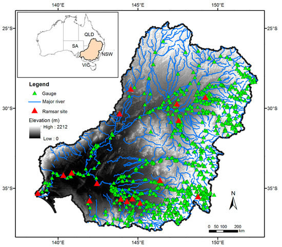
Figure 1.
Study area: the Murray-Darling Basin (MBD).
2.2. Materials
2.2.1. Flow Data
There are over 700 gauges distributed through the MDB (Figure 1). Some of them are maintained by the Murray-Darling Basin Authority (MDBA), and others are maintained by government services of each state, such as New South Wales Office of Water. Observed flow data at these gauges are collected from these agencies and recorded as daily discharge in mega liters per day (ML/day).
2.2.2. WOfS Dataset
The WOfS dataset was acquired from Geoscience Australia’s web service (http://www.ga.gov.au/scientific-topics/hazards/flood/wofs). Each grid cell of WOfS maintains the number of clear satellite observations, the number of water occasions, the percentage of clear observations, and the confidence of water observation. The clear observations are irregular from day to day, from place to place, due to the continuation of Landsat missions and unpredictable cloud cover. Therefore, we generate monthly maximum water maps by overlaying all the observations in a month and selecting all the clear observations of water. Yearly maximum water maps are derived similarly by overlaying all monthly maps of a year. Generation of monthly and yearly maximum water datasets achieves spatially continuous observations by sacrificing the temporal resolution. In this study, WOfS data from 1988 to 2015 were downloaded and used.
3. Methodology
3.1. Constructing a Zone-Gauge Framework
Flood inundation dynamics in the MDB are quite variable across the basin due to the basin’s rich river networks and complex topography. In order to reflect the spatial variation in flood pulses and decrease time lags between flow and inundation, a zone-gauge framework was proposed in the Murray-Darling Basin Floodplain Inundation Modeling (MDB-FIM) projects [37,38], which was later modified by Huang et al. [39] who divided the basin into 90 zones based on a continental scale drainage network product, the Australian Hydrological Geospatial Fabric (Geofabric) published by the Bureau of Meteorology of Australia (http://www.bom.gov.au/water/geofabric/). Each zone was assigned a representative downstream gauge that best records the flow through the zone. Some of the zones were assigned a virtual gauge that was a combination of two or three observed gauges to match as closely as possible to reality. The combination was achieved by addition or subtraction in arithmetic, depending on the location of the gauges. Some of the zones have no clear linkage to the major rivers in the basin and no corresponding gauges. These ungauged zones were excluded in this study because they are generally not inundated.
This study required gauges with observed flow series that are longer than 30 years. Therefore, the original 90-zone framework was modified by merging those zones that have shorter series with others, and a framework with 67 pairs of zones and gauges (Figure 2) was finally adopted in this study. Under this framework, it was assumed that the flood inundation extent in each zone was closely related with the observed flow at its downstream gauge. Higher flow would usually correspond to a larger inundation extent.
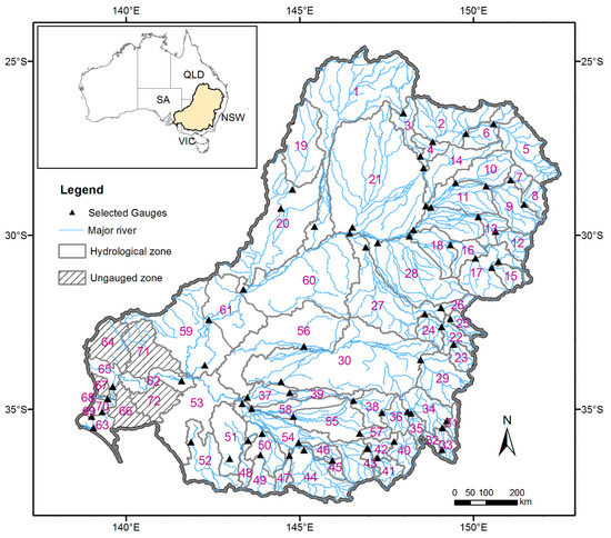
Figure 2.
Hydrological zones and their corresponding gauges.
3.2. Modeling Flood Inundation Dynamics
Spatio-temporal modeling of flood inundation in MDB is based on the zone-gauge framework, which consists of 67 pairs of zones and gauges. Under this framework, inundation extent in each zone was assumed to be closely related with the observed flow at its corresponding gauge. Under this assumption, flood frequency analysis was carried out to the time-series flow data of each gauge based on the annual flood series method, considering that the flow in the study area generally exhibits a pattern of inter-annual variation [22].
An annual flood is defined as the highest peak discharge in a water year. Flood frequency analysis is to estimate the exceedance probability of different flow peaks based on the historic flow peaks. To do that, we should first assume that flow peaks obey some kind of probability distribution. Gumbel distribution is a statistical method often used for predicting extreme events such as earthquake and floods [40]. Therefore, we assume the flow peaks observed at all the gauges fit the Gumbel distribution.
The probability plotting positions are a type of empirical probability distribution and provide appropriate non-exceedance probabilities for the extreme values [41]. While there are many plotting position formulas, such as the California, Hazen, Weibull, and Gringorten methods [42], the Gringorten method [43] was recommended for the Gumbel distribution [42,44,45,46]. Therefore, we have adopted this method. It calculates the Annual Exceedance Probability (AEP) as Equation (1).
where r is the rank of the annual flow peaks from largest to smallest; N is the number of years for the record length.
AEP = (r − 0.44)/(N + 0.12),
According to the date of annual flow peaks, maximum water observation in its corresponding month would be selected, and assigned a value equal to the AEP of this peak to make a probability map. All the probability maps corresponding to each flow peak were then overlaid by taking the maximum probability to generate a final flood inundation probability map. On the other hand, a flood inundation frequency map was derived by simply overlaying all the yearly maximum water observations from 1988 to 2015 and calculating the annual inundated times of each pixel. A flowchart of the modeling process is given in Figure 3.
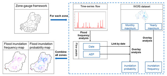
Figure 3.
Flowchart of the modeling process.
4. Results and Validation
4.1. Spatio-Temporal Dynamics of Flood Inundation
4.1.1. Flood Inundation Frequency
Figure 4 shows the inundation frequency in MDB over the period (1988–2015), with each pixel indicating the annual inundated times in these 28 years. Note that it was derived from annually aggregated maximum flood extent, thus intra-annual variability and hydroperiods were not captured. Enlarged areas are four of the Ramsar sites, Narran Lake Nature Reserve, Riverland, Kerang Wetlands, and Currawinya Lakes. This map shows how often an area has been submerged by water. It is clear that frequently inundated areas are generally around river channels. This is because floods in this basin are usually caused by the overbank flow of rivers. Floodplain and wetland ecosystems rely heavily on the overbank flow for water supply. River red gum for example, needs to receive adequate surface flooding periodically to stay healthy [47]. Some aquatic organisms, such as some fish species, also rely on flood pulse to broad their habitats and gain prosperity [48]. Therefore, this resultant map can be a useful indicator for the survival and prosperity of riparian biota communities, which therefore makes it a helpful tool for building knowledge of the relationship between ecosystem conditions and the flooding water.
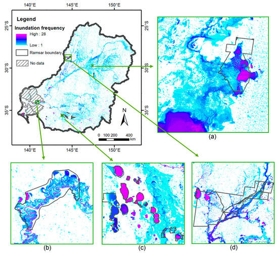
Figure 4.
Flood inundation frequency from 1988 to 2015 in MDB that was derived from annually aggregated maximum flood extent, note that intra-annual variability and hydroperiods are not captured, (a) Narran Lake Nature Reserve, (b) Riverland, (c) Kerang Wetlands (d) Currawinya Lakes.
4.1.2. Flood Inundation Probability
Figure 5 shows the inundation probability that was derived by integrating time series flow data and WOfS product. The probabilities in this map were derived from the AEP of flood frequency analysis, which indicates the probability of a given flow peak being exceeded in any given year. Through combining with corresponding inundation extent that was derived by remote sensing data, it therefore projects future possible inundation based on historic flow and inundation status. The AEP-derived probabilities in this map can be related with another commonly used measurement, the Average Recurrence Interval (ARI). For example, AEP of 0.632 generally equals to a 1-year recurrence interval, and 0.181 equals to a 5-year recurrence interval (Equation (2)). Therefore, the flood inundation probability map can be easily converted into flood inundation maps of different ARIs (Figure 6). From Figure 6, it is observed that most area of the Narran Lake Nature Reserve was inundated at least once every year or every two years, which suggests that its wetlands receives flooding water regularly and frequently. For the Riverland, its wetlands are generally inundated once every five or ten years. Most of the Kerang Wetlands are permanent water bodies that have water cover every year. Except for that, some areas could be inundated by two- or five-year floods. Currawinya Lakes have a relative diverse inundation situation. Wetland areas on the upstream are inundated once every five years, while the downstream wetlands can generally be inundated every two years. The ARI maps can be helpful for pre-formulating future flow regimes to ensure important riparian ecosystems receiving enough water supply. River red gum forests in MDB for example, require flooding water once every five years or more often [49]. As a result, their distribution should be contained within the five year inundation extent, which can be derived from Figure 5 by taking those pixels with probabilities greater than 0.181. Similarly, this resultant map can be useful for identifying other flora and fauna communities that may be in danger due to possible lack of water.
AEP = 1 − Exp(−1/ARI),
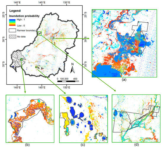
Figure 5.
Flood inundation probability in MDB, (a) Narran Lake Nature Reserve, (b) Riverland, (c) Kerang Wetlands (d) Currawinya Lakes.
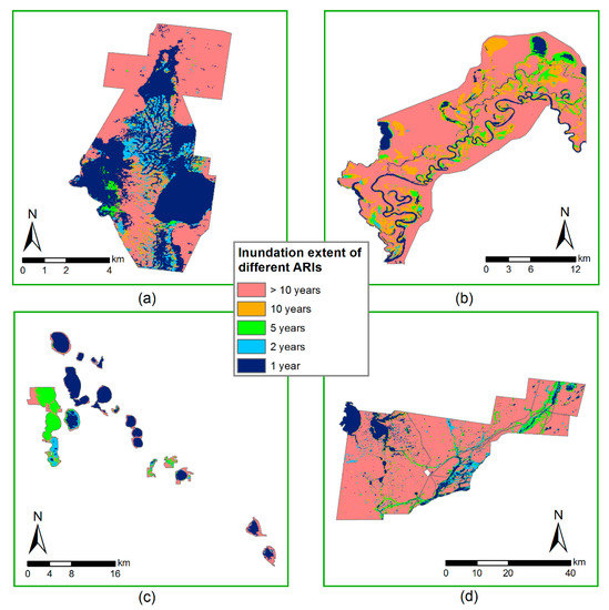
Figure 6.
ARI maps for (a) Narran Lake Nature Reserve, (b) Riverland, (c) Kerang Wetlands (d) Currawinya Lakes.
4.2. Validating the Assumptions
4.2.1. Consistency between Flow and Inundation in Each Zone
The core assumption of this study is that in each zone, the inundation extent is closely related with the observed flow at its complementary gauge. In order to validate this assumption, the inundation area for each month was first calculated and plotted together with daily flow. Figure 7 shows the variation of inundation area (blue line) and flow (red line) from 1987 to 2015 for five demonstration zones. It is clear that flow and inundation in all these zones have similar pattern, with large inundation extent usually accompanying high flow.
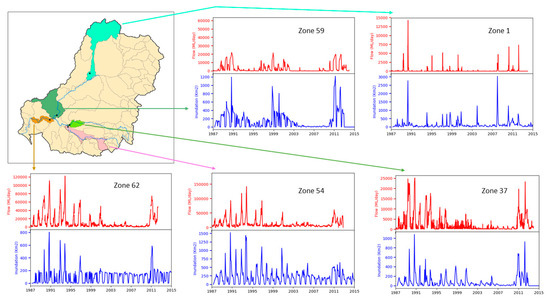
Figure 7.
Time series flow magnitude and remotely sensed inundation area for 5 demonstration zones.
Pearson’s correlation between the flow volume and the inundation area was performed for each zone to further validate the assumption for the whole basin. Pearson’s r and corresponding p-value were calculated and displayed in Figure 8a,b. It can be observed that most of the zones have high r-values with p-values less than 0.05, demonstrating strong consistence between flow and inundation. Zones in the southeast margin of MDB have relatively smaller r values, and some of the zones have high p-values, suggesting a weaker relationship between the inundation extent and flow. After checking their flow and inundation series, it was found that some of these small zones located completely in a stripe that has too many miss Landsat coverages, which leads to non-significant correlations. The other zones are likely to be affected by the more frequent precipitation there. Water that comes from rainfall weakens the agreement between the observed flow magnitude/volume and remotely sensed inundation.
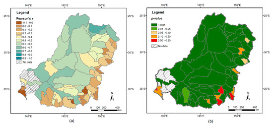
Figure 8.
Correlation between observed flow and remotely sensed inundation in each zone. (a) Pearson’s r; (b) p-value.
4.2.2. Testifying Gumbel Distribution
Another assumption of this study is that the flow peaks fit the Gumbel distribution. The cumulative distribution function of Gumbel distribution is as shown in Equation (3).
where x stands for the volume of flow peaks. Taking logarithm to both sides of this equation, a new equation (Equation (4)) is derived as below.
Here we introduce another variable y calculated as in Equation (5).
Then, y will linearly correlate with x, if flow peaks obey the Gumbel distribution. In Equation (5), independent F(x) values indicate the occurrence probability of a flow that is smaller or equal to x. Therefore, it can be calculated by subtracting AEPs of flow peaks from 1. Linear regression was then conducted to x (flow peaks) and y. Coefficient of determination (R2) was calculated for each zone and displayed on the map (Figure 9). It can be observed that, most of the zones have high R2, except for zone 27 and zone 52, whose coefficients of determination are 0.48 and 0.57 respectively. After checking the flow data of both zones, it was found that zone 27 had an incredibly high flow peak in 1990, corresponding to a major flood event in Macquarie Marshes that year, while most of the flow peaks in zone 52 are 0. This explains why both zones have relatively low R2. Therefore, for the majority of the zones, the Gumbel distribution represents flow peak patterns properly. It is legitimate to assume that the flow peaks in the MDB obey the Gumbel distribution.
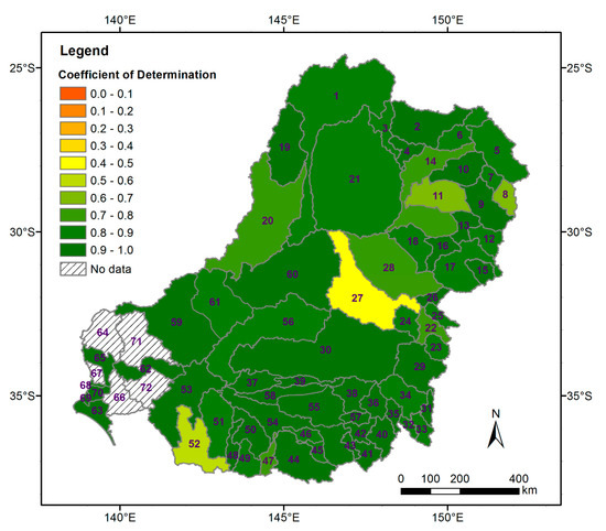
Figure 9.
Coefficient of determination (R2) for the relationship between flow peaks and y in Equation (5).
4.3. Validating Surface Water Observation Dataset
Pekel et al. [30] have mapped global surface water dynamics of the last three decades through the analysis of three million Landsat images using the GEE cloud computing platform, and distributed their results as a Global Surface Water Dataset (GSWD) on the GEE. It was reckoned to have provided the best understanding of the changes in our planet’s surface water [50]. WOfS is also a Landsat-derived surface water dataset that was developed specifically for Australia. Here we want to give a general impression regarding to how big the difference is between both datasets, so that even though we may not be able to find proper references to validate both datasets, cross-validating them would also reveal their reliability to some extent.
An inundation frequency map that records the number of times that a pixel was flagged as water in the annually aggregated water map in the 28 years (1988–2015) was also derived from GSWD using GEE. It was then compared with the inundation frequency map derived from WOfS (Figure 4). Figure 10 shows their difference in the four Ramsar sites. It is clear that both datasets are not exactly the same, with differences existing in all the four sites. However, absolute differences of most pixels are less than 6, suggesting that their differences are in a relatively small range. For the Narran Lake site (Figure 10a), there are some areas that have differences bigger than 7, or even 13. This means that in these areas, WOfS dataset identifies more surface water than GSWD does. Similar situations also exits in the Currawinya Lakes (Figure 10d). Differences in Riverland (Figure 10b) and Kerang Wetlands (Figure 10c) are mostly bigger than −6 and less than 6. Both overestimation and underestimation exit for the WOfS dataset, comparing with the GSWD. It has also to be noted that although both datasets were derived from Landsat imagery, their spatial references are different, which makes their spatial resolutions slightly different. The WOfS has a spatial resolution of approximately 25 m, while the GSWD has a spatial resolution of approximately 30 m. Their difference in spatial resolution would inevitably cause some inconsistences between their inundation frequency maps. This could be one important reason why there are so many differences existing in both frequency maps. Meanwhile, the current comparison was based on annual aggregates. Both datasets could have had entirely different individual surface water maps at any given time step, but these differences could have been masked out entirely in the annual aggregation step. For example, Figure 11 shows a comparison of monthly maximum water observation in WOfS and GWSD under both high flow and low flow scenarios. It is observed that they match well at some sites (e.g., Currawinya Lakes) no matter the flow is high or low. While at some other sites (e.g., Riverland), WOfS dataset tends to miss some tiny in-channel water when the flow is at low level. In this study, since we were only using high flow peaks and their corresponding water observation, this is thus unlikely to affect our modeling accuracy.
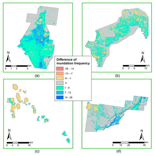
Figure 10.
Differences of inundation frequency in the 28 years detected by WOfS and GSWD at (a) Narran Lake Nature Reserve, (b) Riverland, (c) Kerang Wetlands (d) Currawinya Lakes.
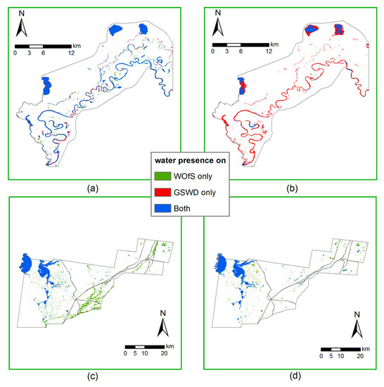
Figure 11.
Differences of monthly maximum water observation in WOfS and GSWD at (a) Riverland with high flow (November 2010), (b) Riverland with low flow (August 2010), (c) Currawinya Lakes with high flow (December 2010), (d) Currawinya Lakes with low flow (September 2010).
5. Discussion
Like many large river basins, the MDB embraces a broad variety of small river systems with unique climate and hydro-morphological characteristics, flow and flooding regimes as well as highly variable levels of river regulation and water abstraction for irrigated agriculture and other uses [51]. This makes the modeling of their flood inundation much more difficult. The zone-gauge framework proposed in MDB-FIM [37,38] and Huang et al. [39], and later adopted by Huang et al. [22] and Heimhuber et al. [31,52], turns out to be an effective way to deal with this difficulty. It is also applicable to other similar large river basins. However, it has to be noted that in the zone-gauge framework, it is important to have a close correlation between inundation extent in each zone and river flow observed at its corresponding gauge. To ensure this, zone delineation and gauge selection need to be carried out very carefully. Even when the correlations are ensured, some other factors may still introduce uncertainties to the proposed model. One is the time lag between gauge flow observation and inundation observation at different areas in the zone. Inundation extent derived from a single remote sensing image can only reflect an instantaneous inundation condition, which makes no single inundation map can be concisely linked to the observed flow. But it is possible to model the time lag based on the grid handling, as achieved by Heimhuber et al. [31]. Another source of uncertainties is the flood frequency analysis on the time series flow data, which is a statistical modeling process that tries to project future flooding regime from historical data. In this study, to deal with the time lag issue, we used monthly maximum water map, which is derived from a composite of images, instead of a single image, to serve the purpose of better matching with observed flow peak. In addition, the assumptions of flood frequency analysis have been carefully validated, in order to prove that uncertainties from this part are manageable.
Except for the modeling processes, the input data themselves also embrace uncertainties. The observed flow data, for example, were normally considered as the most reliable in situ hydrological observations. But there are many different sources of errors that would affect the accuracy of observed flow [53]. For the inundation observation using remote sensing technology, uncertainties are also inevitable. On the one hand, they come from remote sensing data themselves, on the other hand, they come from the interpretation methods. As was demonstrated in the last section, due to different interpretation methods, WOfS and GSWD exhibit differences from place to place, although both were derived from Landsat images.
Unlike the previous study [22] that used MODIS for inundation mapping, this study used a Landsat-derived WOfS dataset, which provides longer time series and higher spatial resolution inundation extents. On the one hand, higher spatial resolution ensures higher accuracy of inundation. Validation results have confirmed the close relation between the inundation and flow. On the other hand, longer time series guarantee more observed inundation samples available, which makes the model more robust. In the meantime, it has also to be noted that the temporal resolution of Landsat may be a limitation for the model. Due to Landsat’s 16-day revisit and cloud cover, peak flood extents would probably often be missed. In this study, we used WOfS monthly maximum water observations to be linked with flow peaks. They have even coarser temporal resolution, but through composition, cloud coverage can be minimized and image quality is significantly improved. Therefore, using monthly composited data is a compromise approach that sacrifices temporal resolution for high image quality. Besides, considering the propagation process of flood inundation, it is legitimate to use a monthly maximum composited water observation to be linked with the flow peak.
Traditional approach for simulating the extent of flooding is through hydrodynamic modeling. Increases in computation power and data availability have led to major advances in continental and even global scale flood modeling in recent years [13]. For example, Schumann et al. [54] applied a hydrodynamic model to generate a 40-year floodplain inundation dynamics across Australia and found good agreement with total inundated areas derived from a Landsat time series. Nevertheless, parameterization of these models remains difficult [55] and accurate representation of complex river and floodplain topographies and the corresponding storage effects is still limited by the quality of suitable datasets such as digital elevation models (DEMs) with global coverage [56]. Moreover, these large-scale hydrodynamic models are still limited for accurately quantifying the complex and fine-scaled dynamics of periodically inundated and potentially shifting inundated areas across large regulated river basins and over long periods of time [18]. Remote sensing technology provides an effective way for quantifying and monitoring surface water dynamics over large areas and long periods of time. With the development of big data and cloud computing technologies, more and more high-quality, long time series, and high-resolution surface water observation datasets can be easily generated. These datasets can be used as valuable input to the hydrodynamic models, or as important reference to calibrate or validate the models [57]. This study proposed a simple but effective model that integrates one of this kind of dataset with flood frequency analysis. It is anticipated that this kind of remote sensing derived dataset could also be integrated with hydrodynamic models to achieve more robust and more reliable flood inundation modeling results.
6. Conclusions
Time series flow observed at gauges provide rich information for studying flood return frequency, but information of spatial extent of flooding is still lacking [58]. Satellite observation is an efficient method for acquiring spatial inundation over large river basins. According to Huang et al. [59], there are three advantages to integrate remotely sensed data with in situ gauge flow data. First, flow data can help select appropriate remote sensing images for flood detection. Second, remote sensing helps flood observation transfer from point-based to region-based. Last, flow data usually have long enough time series for hydrological analysis, which endows remotely sensed inundation hydrological characteristics.
This study proposed a simple but efficient method that integrates time series flow data and a global water observation product to model the flood inundation dynamics. Since a close relationship between flow and inundation is required as the basis of the model, it is important that a large river basin be divided into small hydrological zones first. This is why we adopted the zone-gauge framework for modeling inundation in the MDB. Through validation analysis as described herein, it has been proven that under this framework, the assumptions and basis of the model are tenable for most of MDB. However, it has to be noted that there are still some other uncertainties that may affect the modeling results. For example, inundation variations caused by other drivers other than river dynamics, such as precipitation, groundwater seepage, irrigation, as well as various land and water management strategies, are usually not related to the gauge flow [8]. This would obviously affect the assumption basis of the model.
This study used a Landsat-derived water observation product that has a much longer time series than MODIS data, which obviously would benefit the proposed modeling method. However, the coarse temporal resolution of Landsat would also probably missed rapid inundation, which affects the modeling results. In the future, we are expecting some water observation data sources that have both high spatial resolution and high temporal resolution. This may be acquired from very advanced satellite missions (e.g., CubeSat), or generated through blending multiple data sources, such as MODIS, Landsat, Sentinel-1/2, etc.
As demonstrated in the MDB case study, the proposed modeling method can be applied to any river basin that has a long time series of observed flow data that can be linked to WOfS or any other remotely sensed inundation extent, such as GSWD. The inundation frequency and inundation probability maps show patterns of historic floodplain inundation and projects future possible inundation status. They are useful for revealing water status, estimating water stress and pre-formulating water regime for riverine ecosystems. This method is relatively easy to implement and would provide environmental researchers and managers with important information to assist them for water resource management and wetland ecosystem studies.
Author Contributions
Conceptualization, C.H. and Y.C.; Methodology, C.H.; Software, S.Z.; Validation, L.L., J.S. and Q.L.; Formal analysis, L.L.; Investigation, C.H.; Resources, J.S.; Data curation, Q.L.; Writing—original draft preparation, C.H.; Writing—review & editing, Y.C. and S.Z.; Visualization, C.H.; Supervision, Y.C.; Project administration, C.H.; Funding acquisition, C.H.
Funding
This research was funded by National Natural Science Foundation of China, grant number 41501460, and China Postdoctoral Science Foundation, grant number 2016M600808.
Acknowledgments
We acknowledge MDBA and related government agencies for providing gauge flow data. We are grateful to Geoscience Australia for providing the WOfS product. We also thank Susan Cuddy from CSIRO Land & Water, Australia for kindly reviewing the manuscript.
Conflicts of Interest
The authors declare no conflict of interest. The funders had no role in the design of the study; in the collection, analyses, or interpretation of data; in the writing of the manuscript, or in the decision to publish the results.
References
- Mitsch, W.J.; Gosselink, J.G. The value of wetlands: Importance of scale and landscape setting. Ecol. Econom. 2000, 35, 25–33. [Google Scholar] [CrossRef]
- Prigent, C.; Papa, F.; Aires, F.; Rossow, W.B.; Matthews, E. Global inundation dynamics inferred from multiple satellite observations, 1993–2000. J. Geophys. Res. Atmos. 2007, 112, 1103–1118. [Google Scholar] [CrossRef]
- Papa, F.; Prigent, C.; Rossow, W.B. Ob’ River flood inundations from satellite observations: A relationship with winter snow parameters and river runoff. J. Geophys. Res. Atmos. 2007, 112, D18103. [Google Scholar] [CrossRef]
- Bennett, M.G.; Fritz, K.; Haydenlesmeister, A.; Kozak, J.P.; Nickolotsky, A. An estimate of basin-wide denitrification based on floodplain inundation in the Atchafalaya River Basin, Louisiana. River Res. Appl. 2016, 32, 429–440. [Google Scholar] [CrossRef]
- Ward, D.; Petty, A.M.; Setterfield, S.A.; Douglas, M.M.; Ferdinands, K.B.; Hamilton, S.K.; Phinn, S.R. Floodplain inundation and vegetation dynamics in the Alligator Rivers region (Kakadu) of northern Australia assessed using optical and radar remote sensing. Remote Sens. Environ. 2014, 147, 43–55. [Google Scholar] [CrossRef]
- Balcombe, S.R.; Bunn, S.E.; Mckenziesmith, F.J.; Davies, P.M. Variability of fish diets between dry and flood periods in an arid zone floodplain river. J. Fish Biol. 2005, 67, 1552–1567. [Google Scholar] [CrossRef]
- Phelps, Q.E.; Tripp, S.J.; Herzog, D.P.; Garvey, J.E. Temporary connectivity: The relative benefits of large river floodplain inundation in the lower Mississippi River. Restor. Ecol. 2015, 23, 53–56. [Google Scholar] [CrossRef]
- Allen, Y. Landscape Scale Assessment of Floodplain Inundation Frequency Using Landsat Imagery. River Res. Appl. 2016, 32, 1609–1620. [Google Scholar] [CrossRef]
- Chen, Y.; Huang, C.; Ticehurst, C.; Merrin, L.; Thew, P. An Evaluation of MODIS Daily and 8-day Composite Products for Floodplain and Wetland Inundation Mapping. Wetlands 2013, 33, 823–835. [Google Scholar] [CrossRef]
- Wang, Y.; Colby, J.D.; Mulcahy, K.A. An efficient method for mapping flood extent in a coastal floodplain using Landsat TM and DEM data. Int. J. Remote Sens. 2002, 23, 3681–3696. [Google Scholar] [CrossRef]
- Islam, A.S.; Bala, S.K.; Haque, M.A. Flood inundation map of Bangladesh using MODIS time-series images. J. Flood Risk Manag. 2010, 3, 210–222. [Google Scholar] [CrossRef]
- Thomas, R.F.; Kingsford, R.T.; Lu, Y.; Hunter, S.J. Landsat mapping of annual inundation (1979-2006) of the Macquarie Marshes in semi-arid Australia. Int. J. Remote Sens. 2011, 32, 4545–4569. [Google Scholar] [CrossRef]
- Yamazaki, D.; Kanae, S.; Kim, H.; Oki, T. A physically based description of floodplain inundation dynamics in a global river routing model. Water Resour. Res. 2011, 47, W04501. [Google Scholar] [CrossRef]
- Saf, B. Regional Flood Frequency Analysis Using L Moments for the Buyuk and Kucuk Menderes River Basins of Turkey. J. Hydrol. Eng. 2009, 14, 783–794. [Google Scholar] [CrossRef]
- Seckin, N.; Haktanir, T.; Yurtal, R. Flood frequency analysis of Turkey using L-moments method. Hydrol. Process. 2011, 25, 3499–3505. [Google Scholar] [CrossRef]
- Shi, P.; Chen, X.; Qu, S.M.; Zhang, Z.C.; Ma, J.L. Regional Frequency Analysis of Low Flow Based on L Moments: Case Study in Karst Area, Southwest China. J. Hydrol. Eng. 2010, 15, 370–377. [Google Scholar] [CrossRef]
- Papa, F.; Prigent, C.; Rossow, W.B. Monitoring Flood and Discharge Variations in the Large Siberian Rivers from a Multi-Satellite Technique. Surv. Geophys. 2008, 29, 297–317. [Google Scholar] [CrossRef]
- Alsdorf, D.E.; Lettenmaier, D.P. Tracking fresh waterfrom space. Science 2003, 301, 1491–1494. [Google Scholar] [CrossRef]
- Alsdorf, D.E.; Rodriguez, E.; Lettenmaier, D.P. Measuring surface water from space. Rev. Geophys. 2007, 45, 1–24. [Google Scholar] [CrossRef]
- Frazier, P.; Page, K.; Louis, J.; Briggs, S.; Robertson, A.I. Relating wetland inundation to river flow using Landsat TM data. Int. J. Remote Sens. 2003, 24, 3755–3770. [Google Scholar] [CrossRef]
- Frazier, P.; Page, K. A Reach-scale Remote Sensing Technique to Relate Wetland Inundation to River Flow. River Res. Appl. 2009, 25, 836–849. [Google Scholar] [CrossRef]
- Huang, C.; Chen, Y.; Wu, J. Mapping spatio-temporal flood inundation dynamics at large river basin scale using time-series flow data and MODIS imagery. Int. J. Appl. Earth Obs. 2014, 26, 350–362. [Google Scholar] [CrossRef]
- Ogilvie, A.; Belaud, G.; Delenne, C.; Bailly, J.S.; Bader, J.C.; Oleksiak, A.; Ferry, L.; Martin, D. Decadal monitoring of the Niger Inner Delta flood dynamics using MODIS optical data. J. Hydrol. 2015, 523, 368–383. [Google Scholar] [CrossRef]
- Tulbure, M.G.; Broich, M. Spatiotemporal dynamic of surface water bodies using Landsat time-series data from 1999 to 2011. ISPRS J. Photogramm. 2013, 79, 44–52. [Google Scholar] [CrossRef]
- Tulbure, M.G.; Broich, M.; Stehman, S.V.; Kommareddy, A. Surface water extent dynamics from three decades of seasonally continuous Landsat time series at subcontinental scale in a semi-arid region. Remote Sens. Environ. 2016, 178, 142–157. [Google Scholar] [CrossRef]
- Gorelick, N.; Hancher, M.; Dixon, M.; Ilyushchenko, S.; Thau, D.; Moore, R. Google Earth Engine: Planetary-scale geospatial analysis for everyone. Remote Sens. Environ. 2017, 202, 18–27. [Google Scholar] [CrossRef]
- Lewis, A.; Oliver, S.; Lymburner, L.; Evans, B.; Wyborn, L.; Mueller, N.; Raevksi, G.; Hooke, J.; Woodcock, R.; Sixsmith, J.; et al. The Australian Geoscience Data Cube—Foundations and lessons learned. Remote Sens. Environ. 2017, 202, 276–292. [Google Scholar] [CrossRef]
- Mueller, N.; Lewis, A.; Roberts, D.; Ring, S.; Melrose, R.; Sixsmith, J.; Lymburner, L.; McIntyre, A.; Tan, P.; Curnow, S.; et al. Water observations from space: Mapping surface water from 25 years of Landsat imagery across Australia. Remote Sens. Environ. 2016, 174, 341–352. [Google Scholar] [CrossRef]
- Donchyts, G.; Baart, F.; Winsemius, H.; Gorelick, N.; Kwadijk, J.; Van De Giesen, N. Earth’s surface water change over the past 30 years. Nat. Clim. Chang. 2016, 6, 810–813. [Google Scholar] [CrossRef]
- Pekel, J.-F.; Cottam, A.; Gorelick, N.; Belward, A.S. High-resolution mapping of global surface water and its long-term changes. Nature 2016, 540, 418. [Google Scholar] [CrossRef]
- Heimhuber, V.; Tulbure, M.G.; Broich, M. Modeling Multidecadal Surface Water Inundation Dynamics and Key Drivers on Large River Basin Scale Using Multiple Time Series of Earth-Observation and River Flow Data. Water Resour. Res. 2017, 53, 1251–1269. [Google Scholar] [CrossRef]
- MDBA. Guide to the Proposed Basin Plan: Overview; Murray–Darling Basin Authority: Canberra, Australia, 2010.
- ANCA. A Directory of Important Wetlands in Australia, 2nd ed.; Australian Nature Conservation Agency: Canberra, Australia, 1996.
- Thoms, M.C.; Sheldon, F. Water resource development and hydrological change in a large dryland river: The Barwon-Darling River, Australia. J. Hydrol. 2000, 228, 10–21. [Google Scholar] [CrossRef]
- Ward, J.V.; Tockner, K.; Arscott, D.B.; Claret, C. Riverine landscape diversity. Freshw. Biol. 2002, 47, 517–539. [Google Scholar] [CrossRef]
- CSIRO. Water Availability in the Murray-Darling Basin, A Report to the Australian Government from the CSIRO Murray-Darling Basin Sustainable Yields Project; CSIRO Publishing: Canberra, Australia, 2008. [Google Scholar]
- Overton, I.; Doody, T.; Pollock, D.; Guerschman, J.P.; Warren, G.; Jin, W.; Chen, Y.; Wurcker, B. The Murray-Darling Basin Floodplain Inundation Model (MDB-FIM). Report for the Murray-Darling Basin Authority; CSIRO Water for a Healthy Country Flagship: Canberra, Australia, 2010. [Google Scholar]
- Chen, Y.; Cuddy, S.M.; Merrin, L.E.; Huang, C.; Pollock, D.; Sims, N.; Wang, B.; Bai, Q. Murray-Darling Basin Floodplain Inundation Model Version 2.0 (MDB-FIM2). Report for the Murray-Darling Basin Authority; CSIRO Water for a Healthy Country Flagship: Canberra, Australia, 2012. [Google Scholar]
- Huang, C.; Chen, Y.; Wu, J. GIS-based spatial zoning for flood inundation modelling in the Murray-Darling Basin. In Proceedings of the 20th International Congress on Modelling and Simulation (MODSIM2013), Adelaide, Australia, 1–6 December 2013. [Google Scholar]
- Waylen, P.; Woo, M.-K. Regionalization and prediction of annual floods in the Fraser River catchment, British Columbia. J. Am. Water Resour. Assoc. 1981, 17, 655–661. [Google Scholar] [CrossRef]
- Kang, D.; Ko, K.; Huh, J. Determination of extreme wind values using the Gumbel distribution. Energy 2015, 86, 51–58. [Google Scholar] [CrossRef]
- Cunnane, C. Unbiased plotting positions—A review. J. Hydrol. 1978, 37, 205–222. [Google Scholar] [CrossRef]
- Gringorten, I.I. A Plotting Rule for Extreme Probability Paper. J. Geophys. Res. 1963, 68, 813–814. [Google Scholar] [CrossRef]
- Guo, S.L. A discussion on unbiased plotting positions for the general extreme value distribution. J. Hydrol. 1990, 121, 33–44. [Google Scholar] [CrossRef]
- Kim, S.; Shin, H.; Joo, K.; Heo, J.-H. Development of plotting position for the general extreme value distribution. J. Hydrol. 2012, 475, 259–269. [Google Scholar] [CrossRef]
- Selaman, O.S.; Said, S.; Putuhena, F.J. Flood frequency analysis for Sarawak using Weibull, Gringorten and L-moments formula. J. Inst. Eng. 2007, 68, 43–52. [Google Scholar]
- Rogers, K.; Ralph, J.T. Floodplain Wetland Biota in the Murray-Darling Basin: Water Habitat Requirements; CSIRO Publishing: Victoria, Australia, 2010. [Google Scholar]
- Pringle, C. What is hydrologic connectivity and why is it ecologically important? Hydrol. Process. 2003, 17, 2685–2689. [Google Scholar] [CrossRef]
- Steenbeeke, G.; Kidson, R.; Witts, T.; Brereton, G. A Review of Recent Studies Investigating Biological & Physical Processes in the Macqarie Marshes; NSW Department of Land and Water Conservation: Sydney, Australia, 2000.
- Yamazaki, D.; Trigg, M.A. Hydrology: The dynamics of Earth’s surface water. Nature 2016, 540, 348–349. [Google Scholar] [CrossRef] [PubMed]
- Leblanc, M.; Tweed, S.; Van Dijk, A.; Timbal, B. A review of historic and future hydrological changes in the Murray-Darling Basin. Glob. Planet. Chang. 2012, 80–81, 226–246. [Google Scholar] [CrossRef]
- Heimhuber, V.; Tulbure, M.G.; Broich, M. Modeling 25 years of spatio-temporal surface water and inundation dynamics on large river basin scale using time series of Earth observation data. Hydrol. Earth Syst. Sci. 2016, 20, 2227–2250. [Google Scholar] [CrossRef]
- Di Baldassarre, G.; Montanari, A. Uncertainty in river discharge observations: A quantitative analysis. Hydrol. Earth Syst. Sci. 2009, 13, 913–921. [Google Scholar] [CrossRef]
- Schumann, G.J.; Stampoulis, D.; Smith, A.M.; Sampson, C.C. Rethinking flood hazard at the global scale. Geophys. Res. Lett. 2016, 43, 10249–10256. [Google Scholar] [CrossRef]
- Ticehurst, C.; Dutta, D.; Karim, F.; Vaze, J. Validation of surface water maps in selected Australian floodplains derived from Landsat imagery using hydrodynamic modelling. In Proceedings of the 22nd International Congress on Modelling and Simulation (MODSIM2017), Hobart, Australia, 3–8 December 2017. [Google Scholar]
- Bates, P.D.; Neal, J.C.; Alsdorf, D. Observing global surface water flood dynamics. Surv. Geophys. 2014, 35, 839–852. [Google Scholar] [CrossRef]
- Fleischmann, A.; Siqueira, V.; Paris, A.; Collischonn, W.; Paiva, R.; Pontes, P.; Crétaux, J.F.; Bergé-Nguyen, M.; Biancamaria, S.; Gosset, M.; et al. Modelling hydrologic and hydrodynamic processes in basins with large semi-arid wetlands. J. Hydrol. 2018, 561, 943–959. [Google Scholar] [CrossRef]
- Theiling, C.H.; Burant, J.T. Flood inundation mapping for integrated floodplain management: Upper Mississippi River system. River Res. Appl. 2013, 29, 961–978. [Google Scholar] [CrossRef]
- Huang, C.; Chen, Y.; Zhang, S.; Wu, J. Detecting, Extracting, and Monitoring Surface Water from Space Using Optical Sensors: A Review. Rev. Geophys. 2018, 56, 333–360. [Google Scholar] [CrossRef]
© 2019 by the authors. Licensee MDPI, Basel, Switzerland. This article is an open access article distributed under the terms and conditions of the Creative Commons Attribution (CC BY) license (http://creativecommons.org/licenses/by/4.0/).