Abstract
As the world population keeps increasing and cultivating more land, the extraction of vegetation conditions using remote sensing is important for monitoring land changes in areas with limited ground observations. Water supply in wetlands directly affects plant growth and biodiversity, which makes monitoring drought an important aspect in such areas. Vegetation Temperature Condition Index (VTCI) which depends on thermal stress and vegetation state, is widely used as an indicator for drought monitoring using satellite data. In this study, using clear-sky Landsat multispectral images, VTCI was derived from Land Surface Temperature (LST) and the Normalized Difference Vegetation Index (NDVI). Derived VTCI was used to observe the drought patterns of the wetlands in Lake Chad between 1999 and 2018. The proportion of vegetation from WorldView-3 images was later introduced to evaluate the methods used. With an overall accuracy exceeding 90% and a kappa coefficient greater than 0.8, these methods accurately acquired vegetation training samples and adaptive thresholds, allowing for accurate estimations of the spatially distributed VTCI. The results obtained present a coherent spatial distribution of VTCI values estimated using LST and NDVI. Most areas during the study period experienced mild drought conditions, though severe cases were often seen around the northern part of the lake. With limited in-situ data in this area, this study presents how VTCI estimations can be developed for drought monitoring using satellite observations. This further shows the usefulness of remote sensing to improve the information about areas that are difficult to access or with poor availability of conventional meteorological data.
1. Introduction
Marshes and vegetation close to inland water bodies are known to be sensitive to changes in hydrology within their natural habitat since they co-exist in transitional zones between aquatic and terrestrial systems. Shortage of water availability leads to soil moisture depletion, which further hinders the growth and health of plants in the area [1]. Increases in temperature also affect these vegetation systems by accelerating their rate of evaporation and transpiration [2]. Though information on rainfall, surface and groundwater patterns are required for understanding and management of a given environment, this information is insufficient on its own. Interaction with various environmental and social factors such as floods, droughts, bushfires, irrigation and many others also need to be taken into account.
Drought is one of the most damaging weather-induced disasters. Timely information of its duration, spatial coverage, intensity and impact is essential for drought management. Droughts often result in the loss of livelihoods coupled with numerous environmental impacts, particularly in the agricultural sector [3,4,5]. Given that marshes and vegetation close to inland water bodies are tied to the availability of water within their ecosystem, identification of drought patterns could be used as a tool for monitoring and sustainable management [6]. Drought monitoring becomes a hurdle in cases where the wetland and marshes are in hard-to-reach areas and with occasional unfavorable flooding conditions. This coupled with limited and low-quality ground observations hinders effective drought monitoring for a given area.
A drought index can help to define drought parameters such as severity, duration intensity and spatial extent. For a given environment, this index assimilates different meteorological and hydrological parameters, as well as water supply indicators into a single numerical value and gives a comprehensive representation for that environment. This comprehensive representation is readily useable rather than raw data. Its numerical values are usually used by decision and policy makers to evaluate and monitor drought situations. Therefore, creating a time series of a drought index can provide a “framework” for evaluating those parameters. Numerous indices have been developed for drought representation. They have been broadly divided into two categories; site-based and remote sensing-based indices [7,8].
The site-based indices use multiple hydro-meteorological variables in a single drought indicator to capture the interactions that lead to droughts. Common types of site-based drought indices include, the Palmer Drought Severity Index (PDSI), which is a popular meteorological drought index that uses precipitation and temperature to monitor soil moisture changes within a two-layer water balance model. PDSI values typically vary from −4.0 to +4.0, negative values indicating drought conditions, while positive values indicate wet conditions [9]. Another drought index that is popular because of its computational simplicity and forecasting ability at different time scales is the Standardized Precipitation Index (SPI). The SPI first fits a probability distribution to historic precipitation time-series data, and then normalizes the fitted distribution using the standard inverse Gaussian function to compute the drought index. SPI values are dimensionless with negative values indicating drought conditions, and the magnitudes of their departures from zero indicating the severity of the drought [10]. The accuracies of drought indices like the PDSI, and SPI depends on ground observations. Such dependencies become unreliable in areas where these observations are sparse and usually of poor temporal resolution [11]. At a regional scale, drought indices derived from in situ precipitation and temperature cannot provide insight on spatial variability in drought conditions [12].
Over the years, satellite remote sensing products have provided numerous affordable and efficient monitoring tools for mapping and describing environmental changes from a local to a global scale [13,14]. Remote sensing-based indices typically use observations in several spectral bands, each of which provides different information about surface conditions at varying times. Some remote sensing-based indices includes; Normalized Difference Vegetation Index (NDVI), Temperature Condition Index (TCI), Vegetation Condition Index (VCI), Vegetation Health Index (VHI). TCI, VCI, and VHI are known as vegetation indices which are often used as drought indicators. TCI identifies vegetation stress caused by extreme hot and wet conditions. VCI is used to classify vegetation changes from “bad” to “optimum” condition while the VHI describes vegetation health from the combination of TCI (temperature) and VCI (vegetation condition) [13]. Some of these drought indices and indicators have been used by international organizations to produce and maintain online drought monitoring platforms. An example of these platforms is the Global Vegetation Health system. It is managed by the Center for Satellite Application and Research (NOAA STAR) and estimates vegetation health, moisture and thermal conditions. Its VHIs are derived from the radiance observed by the Advanced Very High-Resolution Radiometer (AVHRR) and provides its products at 4 km spatial resolution. Some other efforts like the Global Information and Early Warning System on Food and Agriculture (FAO-GIEWS) provides monthly briefings on countries under drought that are facing food crisis (http://www.fao.org/giews/en/). For the African continent, the U.S. Agency for International Development (USAID) Famine Early Warning System Network (FEWS Net) (https://earlywarning.usgs.gov/fews) produces and maintains several drought monitoring indicators including SPI, evapotranspiration and NDVI products. Remote sensing data are used to generate these indicators. The product resolution for this area ranges from a scale of 250 m to 10 km. While these outputs are valuable, seasonal drought variations derived at a higher resolution for a specific area in need can substantially improve risk assessment.
Since droughts are naturally associated with vegetation state and cover, vegetation indices (VI) are commonly used as an indicator for drought monitoring [15,16]. For a given area, the absorption and reflection of photosynthetically active radiation over a period of time can be used to characterize the health of the vegetation that area. This can be achieved by using NDVI, which is the most commonly used VI indicator for drought monitoring. It has been extensively used in ecosystem monitoring and particularly as a drought indicator even in environments where vegetation cover was less than 30% [17,18,19]. Some researchers have used NDVI to monitor drought on a national scale. For example, Nanzad et al. [20] mapped out drought severity for Mongolia during the “growing” season using NDVI [21].
Land Surface Temperature (LST) can provide valuable information about the hydrological setting of an environment. High LST values usually depict extreme dry conditions due to a lack of soil moisture. When used together, NDVI and LST products can provide insight for drought monitoring. Such a combination may help to infer water stress in bare land, sparse and fully vegetated area [22,23]. For pixels with the same NDVI, a low LST value will represent stronger evaporative cooling. This is because there is sufficient water which enhances transpiration and cools plants. In contrast, a water deficient plant will experience an increase in leaf temperature due to closing of the plant stomata.
Following the Lake Chad’s drastic decrease in water levels, numerous studies have been carried out on the hydrology of the Lake Chad Basin (LCB). With the lack of in situ observations in this area, most of the studies relied on various satellite products to document hydrological changes [24,25]. Some researchers used satellite products to analyze precipitation trends and its effects on lake levels in Komadugu-Yobe which is a river that flows into Lake Chad through Nigeria and Niger [26,27]. The effects of regional precipitation variations and the impact of anthropogenic activities on Lake Chad was reported by Coe and Foley [28]. Other researchers focused on water availability and spatio-temporal variability of water storage over the LCB. For example, Coe and Birkett [29], used satellite radar altimetric lake height measurements to estimate river discharge.
Unlike the hydrological aspects of the lake, studies on drought conditions of the LCB are relatively few. Approximately three sources were found to provide significant studies on drought over the basin. Nkiaka et al. [30] used Standardized Precipitation Index (SPI) and Standardized Streamflow Index (SSI) to analyze dry/wet conditions in the Logone catchment over a 50-year period (1951–2000). Their results revealed both the Sudano and Sahelian zones are equally prone to droughts and floods. Ndehedehe et al. [31] used recently introduced standardized non-parametric univariate and multivariate drought indices for the characterization of different droughts. They used the Independent Component Analysis (ICA), a higher order statistical technique to decompose SPI and standardized soil moisture index values into spatial and temporal patterns. The authors further used the multivariate standardized index (MSDI) to evaluate the effectiveness of rainfall and soil moisture in capturing drought frequency, persistence, and termination. Though marked with variability, the authors recorded relatively wet conditions for the last two decades from the temporal evolutions of SPI at 12 months aggregate. Okonkwo et al. [32] analyzed monthly gridded rainfall using SPI to show that extreme wet conditions prevailed within the basin in 2010. Using autocorrelation analysis, the authors identified a high drought index in the northernmost part of the LCB and suggested a higher likelihood of low rainfall in that area. Though very insightful, these studies either generalized for the entire LCB which has an area of about 2.5 × 10⁶ km2 or used ground observations in computing the drought indices. Drought indices derived from such data for that large an area cannot provide information on the regional drought intensity or patterns for this area. Additionally, for an area like Lake Chad where recent ground observation stations are sparse, these data sets may not be available in time for drought monitoring and decision making. For instance, with regards to the water transfer project to replenish the lake, such indices may not be able to provide near to real time regional drought patterns within the LCB. Such information could help authorities determine where and when water is to be transferred from the Congo Basin into the LCB.
Last year, UNESCO launched the BIOsphere and Heritage of Lake Chad (BIOPALT) project. The project aims to strengthen the capacity of member states of the Lake Chad Basin Commission (LCBC) to monitor and sustainably manage the hydrological, biological and cultural resources of the LCB [33]. A major objective of this project is to establish an early warning system for droughts and floods in the Lake Chad area. Seasonal drought variation patterns have the potential to provide vital information to such a warning system. With farming and animal grazing being predominant activities among inhabitants in this area, such information also has the potential of helping locals to make adaptive choices on planting seasons, crop varieties and labor usage. Therefore, understanding the drought severity on the immediate environment of the lake will be a useful and robust tool for planning and development strategies.
The overall goal of this study is to characterize spatial drought patterns in the immediate environment of Lake Chad during the dry seasons of 1999, 2007, 2010, 2013, 2015, and 2018. This will be achieved by deriving Land Surface Temperature (LST) and vegetation information as indicators for drought monitoring from Landsat images with a spatial resolution of 30 m. First, both NDVI and LST datasets were obtained using Landsat satellite images. Later, the VTCI was produced, identifying drought zones for this area. For authorities to be able to address the underlying drivers of any future environmental crisis, the environmental changes occurring within and around the lake must be understood across multiple spatial and temporal scales. This has the potential of providing authorities with up-to-date data needed to execute the water transfer and the BIOPALT projects which all aim to restore the degraded ecosystems in this area.
2. Study Area
2.1. General Overview
The Lake Chad Basin (LCB) is one of the largest inland drainage basins covering about 2,500,000 km2 and supports over 30 million people for various purposes [34]. At its center, lies Lake Chad, a freshwater body that is shared between Cameroon (CMR), Chad (TCD), Nigeria (NGA), and Niger (NER) as seen in Figure 1. The lake receives most of its water supply from the Chari-Logone River with over 90% of inflows into the southern section of the lake. The Komadugu-Yobe River provides about 3% of water that flows into the lake from the northern section and is highly dependent on rainfall [26,30]. In a little over forty years, Lake Chad lost about 90% of its water (24,000 km2~1700 km2) with most of this decrease occurring between the years 1973 and 1975. [35,36]. Due to severe droughts during that period, the lake was separated into two parts with a great sand barrier lying between the southern part which has always had a pool of open water, and the northern part which is sometimes inundated [35]. The decrease in water levels led to the emergence of different land surface features within Lake Chad. Vegetation is the major land surface feature in this area occupying about 55% of what used to be open water in this area. Followed by patches of sand dunes which occupies about 35% of the area. Marshes which are mostly found around the transition areas between water and sand dunes, covers about 15% of this area. Open water makes up the remaining 10% [24].
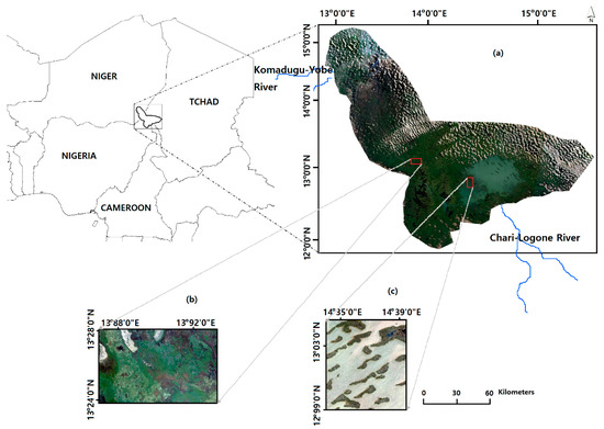
Figure 1.
Study area ((a) represents the focus area, (b,c) are high resolution images from WorldView-3 used for validation purposes).
The population within the LCB is estimated to reach 80 million by 2030 and with this increase, there is an anticipated increase in demand for water and various economic and livelihood activities linked to it [37]. Numerous studies have shown considerable fluctuations in lake levels over the past decades. Some authors attributed these fluctuations to climate variability and environmental degradation [19,27,28,29].
2.2. Climate and Hydrology
The LCB climate is characterized by high spatio-temporal variability in rainfall which is mostly controlled by oceanic and continental regimes from the south and north, respectively. The LCB experiences its highest temperatures between February and June where it sometimes reaches 40 °C, representing the hottest period in this area (Figure 2). The lowest temperatures in this area are recorded between October and January. The average annual temperature in this area ranges between 30 °C and 40 °C. Rainfall in this area lasts from June through September and the rest of the year is relatively dry [35]. The lake’s mean depth during extreme conditions varies between 0–1.8 m in the northern pool and about 0.5–2 m in the southern pool [29]. The lake has a very obvious seasonal variation in precipitation with ~90% of the annual precipitation accounted for during the rainy season.
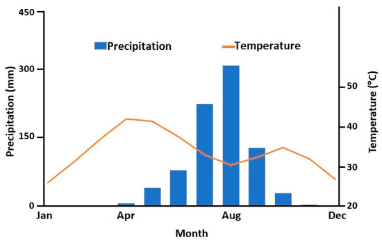
Figure 2.
Mean Monthly precipitation and mean monthly air temperature in Lake Chad.
Rainfall variability has also been attributed to a decline in the area of Lake Chad [31]. During the early 1960′s, rainfall over the basin decreased significantly while irrigation (bolstered by the demographic growth) flourished over the same period [27]. It is reported that the reason why the lake has been especially vulnerable to climate variability is because of its rather shallow depth of less than 7 m [26,32].
3. Materials and Methods
3.1. Materials
With a relatively high spatial resolution of 30 m, Landsat images have been widely used to study and monitor various aspects of inland water bodies [38,39]. It has provided unparalleled global coverage at medium resolution for over 40 years.
Using the bulk download, 392 images were initially downloaded for the dry season (November to March) periods of 1999, 2007, 2010, 2013, 2015, and 2018 from the USGS Glovis data archive (https://glovis.usgs.gov). The six dry season periods were selected based on image availability and to represent each Landsat sensor. After visually inspecting the downloaded images, a total of 126 images acquired from Landsat 5 Thematic Mapper (TM), 7 Enhanced Thematic Mapper Plus (EMT+), and Landsat 8 Operational Land Imager (OLI) were selected for processing (Figure 3). The scan line corrector (SLC) of the ETM+ sensor on board Landsat-7 failed permanently, causing a loss of about 17% of the SLC-off image data. A local histogram matching technique proposed by the USGS was used to fill the gaps [40]. Gap filling was carried out for each affected image using the landsat_gapfill.sav extension toolbox in ENVI. Radiometric calibration and atmospheric correction were carried out on the images to eliminate errors from sensors, atmospheric scattering, absorption and reflection. Four Landsat scenes (Path/Row: 184/51, 185/50, 185/51 and 186/50) needed to be mosaicked to generate a “complete” region of interest.
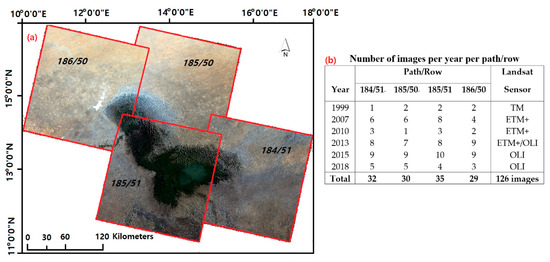
Figure 3.
(a) Shows the number of scenes needed to make a “complete” study area. (b) Shows the number of images per year per path/row used for processing.
For validation purposes, two very high-resolution multispectral images acquired from WorldView-3 (WV-3) were used to validate the reliability of the method used in this study. WV-3 is a high spatial and spectral resolution (0.31 m panchromatic, 1.24 m multispectral resolution) satellite which has an average revisit time of 1.1 days.
3.2. Methods
3.2.1. Landsat Preprocessing
Landsat data must be preprocessed prior to analysis of any kind. Using ENVI 5.3 software, various steps were taken to accomplish the preprocessing phase of this study. Landsat scenes were screened to remove cloud/cloud shadows and converted to Top-of-Atmosphere (TOA) reflectance with the help of information from each scene’s metadata file. A detailed explanation of Landsat preprocessing steps for this area is presented in [24].
3.2.2. Normalized Difference Vegetation Index (NDVI)
The NDVI is a numerical indicator that represents the health of a vegetation canopy and it is wildly used as a measure of vegetation changes [17,18,19]. Healthy vegetation absorbs most of the visible light while reflecting most of the near-infrared light. Unhealthy vegetation reflects most of the visible light and less near-infrared. Given this information, NDVI can be derived by using bands that are sensitive to vegetation information. It can be computed using Equation (1).
where ρNIR is the reflectance of the near-infrared wavelength band and ρred is the reflectance of the red wavelength band.
Theoretically, NDVI values are represented as a ratio ranging from -1 to 1. Higher NDVI values usually represent “greener” plants with greater photosynthetic capacity within a vegetation canopy. NDVI for each Landsat image is required to calculate their emissivity which is used to compute Land Surface Temperature (LST).
3.2.3. Deriving LST
Using top of the atmosphere radiance from the thermal infrared sensors, it is possible to calculate brightness temperatures by applying Plank’s law [41]. For this estimation, thermal bands from the multispectral images are needed. This is band 6 for Landsat 5 and 7, and band 10–11 for Landsat 8. Their respective wavelengths are presented in Table 1.
where T is brightness temperature in Kelvin (K), Lλ is spectral radiance at the sensor’s aperture, K1 and K2 are the calibration constants. For Landsat 5, K1= 607.76 Wm−2 sr−1 μm−1 and K2 = 1260.56 (Kelvin); for Landsat 7, K1 = 666.09 Wm−2 sr−1 μm−1 and K2 = 1282.71 (Kelvin); for Landsat 8, K1 = 774.89 Wm−2 sr−1 μm−1 and K2 = 1321.08.

Table 1.
Landsat bands and wavelength for Land Surface Temperature (LST) calculation.
Temperature values obtained from Equation (2) above are referenced to a black body and must be corrected before VTCI can be calculated. Emissivity corrected values were estimated using the NDVI threshold method [42]. To compute emissivity, the proportion of vegetation, (PV), of each pixel was determined from NDVI using the following equation.
where NDVImin is the minimum NDVI value (<0.2) where pixels are considered to be soil and NDVImax is the maximum NDVI value (>0.5) where pixels are considered to be healthy vegetation. In a case where a pixel is composed by a mixture of soil and vegetation (0.2 ≤ NDVI ≤ 0.5), emissivity is calculated according to the following equation [42].
is vegetation emissivity, is soil emissivity, is proportion of vegetation and is the effect of the geometrical distribution of the natural surfaces and internal reflections. For heterogeneous surfaces, could be 2%. An approximation of the term is given by;
where F is a shape factor whose mean, assuming different geometrical distribution, is 0.55 [43]. Taking into account Equations (4) and (5), emissivity can be calculated as:
Finally, the LST was derived using the following equation [41];
where , h is Planck’s constant (6.626 ∗ 10−34 J s), c is the velocity of light (2.998 ∗ 108 ms−1), and σ is the Boltzmann constant (1.38 ∗ 10−23 JK−1). ε is the emissivity derived from NDVI. The values for the wavelength of emitted radiance (λ) for different thermal bands are listed in Table 1.
3.2.4. Deriving Vegetation Temperature Condition Index (VTCI)
Canopy temperature and water content serve as indicators reflecting the health condition of vegetation. VTCI can be used to describe the water stress condition of a pixel. It is usually derived from the changes in both LST and NDVI, based on an LST-NDVI space relation. This space relation can be established by using a scatter plot of each composite image of LST and NDVI to analyze the wet and dry conditions within an area (Figure 4). The straight lines are drawn in the scatter plots based on the scatter plots of each LST and NDVI products. The upper and lower limits of the respective scatter plots represent the ‘warm edges’, and ‘cold edges’, respectively.
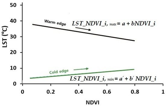
Figure 4.
Parametrization of LST_NDVI_i,max and LST_NDVI_i,min from LST-NDVI scatterplot.
In the LST-NDVI space from a given composite product, some pixels have similar NDVI values yet different LSTs. Therefore, a maximum LST and a minimum LST is available for each NDVI value in theory. The warm and cold edges were obtained from the scatter plots by sorting both maximum and minimum LST for each small interval of NDVI (0.01). For this study, scatter plots of the different composite NDVI and LST products were made using ENVI image processing software. The maximum LSTs vary along with NDVIs and can be linearly regressed using Equation (8). The regression line is called the “warm edge” (water stress restriction), while the regression line between the minimum LST and NDVI (Equation (9)) is called the “cold edge” (no water limitation) of the triangle (Figure 4).
LST_NDVI_i,max and LST_NDVI_i,min are the maximum and minimum LSTs, respectively, of pixels that have the same NDVI value. Coefficients a, b, a′, and b′ can be estimated from linear regression utilizing maximum and minimum values of NDVI and the associated LST values within the image domain.
To obtain accurate a, b, a′, and b′ which are crucial for measuring VTCI, the region used for building the LST-NDVI space must be large enough to represent a wide range of NDVI and LST. This range should be comprised of surface moisture contents from wet to dry and from bare soil to a fully vegetated surface. From such a wide range, it is possible to accurately estimate coefficients a, b, a′, and b′ from the scatter plot of the LST and NDVI in the study area. The shape of the scatter plot is normally triangular or trapezoidal if the study area is large enough to provide a wide range of NDVI and LST [44]. In Figure 4, a and a′ are the intercept and b and b′ are the slope of the warm edge and cold edge, respectively. VTCI was then calculated for each pixel using Equation (10).
where and are obtained using Equations (8) and (9), respectively.
In Equation (10), the denominator is computed as the difference between the maximum () and minimum LSTs () for the specified NDVI_i, while the numerator is computed as the difference between the maximum and current pixel LSTs (LST_NDVI_i) for a given composite product.
VTCI rescales the vegetation dynamics between 0 and 1 to reflect relative changes in vegetation condition from “bad” (indicating a condition with relatively less soil moisture, corresponding to a relatively limited evaporation, and plants are considered as suffering water-stress conditions), to “good” (indicating a condition with minimum water restriction or maximum transpiration for plant growth) [44]. Therefore, a high VTCI value corresponds to healthy vegetation while a low VTCI value corresponds to a stressed vegetation [45]. VTCI drought levels can be categorized into five levels, as seen in Table 2 [46,47]
Table 2.
Classification of Vegetation Temperature Condition Index (VTCI) values in terms of drought.
3.2.5. Performance Evaluation
Vegetation information from Landsat images is mainly interpreted by differences and changes of the green leaves from plants and canopy spectral characteristics. NDVI was used to characterize canopy growth or vigor which is indicative of vegetation health. However, NDVI is sensitive to the effects of soil brightness, soil color, atmosphere, cloud and cloud shadow, and leaf canopy shadow. NDVI for each Landsat image in this study is required to calculate their respective proportion of vegetation (Pv) which is needed for the computation of emissivity values. Hence, faulty NDVI values will result in faulty VTCI estimates. The most common validation process of a vegetation index is through direct correlations with vegetation characteristics of interest measured in situ, such as vegetation cover, biomass, growth, and vigor assessment. Considering the size and location of the study area, it is difficult to obtain accurate ground-truth observational data on soil moisture, vegetation cover or health. Therefore, to evaluate the reliability of the drought estimation method used in this study, Pv composite images prepared from high resolution WV-3 images were used to create reference maps for comparison with those from Landsat. Pv can be calculated using Equation (3).
Since most of the lake area is located within the tile path/row 185/51 (Figure 3), the WV-3 reference images were selected within this tile and their vegetation extent were outlined as being the “true” extent. Due to price constraints, two WV-3 images were used for this purpose (Table 3). However, using visual inspection, the two WV-3 images were selected to represent the heterogeneous landscape in this area. We made sure it was easy to identify vegetation, marshes, water and soil features within each image as well as transition zones between the features.
Table 3.
Description of Landsat 8 and corresponding reference WV-3 scenes.
Before quantitative analysis, remote sensing data should be converted to absolute surface reflectance. Using the metadata files associated with each image, WV-3 images were atmospherically corrected by transforming digital numbers (DN) to at-sensor radiance values in the unit of W m−2 sr−1 µm−1. This was carried out using ENVI image analysis software. About 100 homologous ground control points (GCPs) were selected on each WV-3 image. Image rectification was based on cubic convolution resampling and polynomial transformation and set to WGS 84/UTM zone 33 N projection. The geometrically-corrected Worldview-3 images were subsequently used as references to correct the Landsat images.
Vegetation proportion composite products prepared from WV-3 images were used to generate reference maps needed to evaluate how accurate our drought estimation method was. It should be noted that, even though WV-3 has a revisit time of 1.1 days, an area might not have data records at every 1.1 days interval. This explains the difference in acquisition dates of the images in Table 3. Nonetheless, there was no severe drought or flooding event reported in this area during those months.
Reference points were selected from the WV-3 images through visual inspection and stratified random sampling was applied to represent a range of different vegetation conditions. The Landsat-derived vegetation proportion records were extracted for the selected points and compared to that of WV-3. The sampling probabilities were applied as weights for unbiased estimations for the region of interest. Given the heterogeneity of the landform in this area, a uniform minimum and maximum NDVI values could not be used for the estimation of vegetation proportion. Using the same value across all the images may lead to the misclassification of some pixels. The minimum and maximum NDVI values for this purpose were therefore obtained from each NDVI composite product. As such, the resulting vegetation proportion composite images contained pixels from different land surface features. The boundaries of the vegetation feature were extracted from the composite image by manually training each image into “vegetation” and “other” polygons using a supervised classification. The vector polygons were then converted to raster data. Since WV-3 images have a much higher spatial resolution (1.24 m) than the resolution of the Landsat products (30 m), we up-sampled the Landsat products to match the resolution of the reference products. This approach reduced the loss of information and enabled us to carry out a per pixel comparison to assess the accuracy of the vegetation proportion products. The extracted products were classified into four categories and could either be; True Positive or True Negative which will represent image pixels that are correctly classified as vegetation or non-vegetation respectively, and, False Positive or False Negative which denotes image pixels that were mistakenly classified as vegetation and non-vegetation respectively. Using these classes, an error matrix table of class labels allocated by the pixel classification of the Landsat derived pixels against the referenced WV-3 derived pixels was created. More detailed information on spatial accuracy assessment and confusion matrix can be found in [46,47].
The accuracy parameters derived from populating the error matrix table for this study included the Overall Accuracy (OA), Commission Errors (CE), Omission Errors (OE) and the kappa coefficient (k) of agreement. The OA provides the probability that a randomly selected sample on the image is correctly classified. CE occurs when a feature is incorrectly included in the category being evaluated. OE represents features that are left out of the category being evaluated. The Kappa coefficient measures the percentage of agreement between the referenced WV-3 vegetation proportion pixels and segmented Landsat vegetation proportion pixels. OA, CE, OE and k can be calculated using Equations (11)–(14) respectively.
where, P = total number of pixels in the reference data, Pai = total number of correct pixels of the ith category, Pic = total number of pixels for the ith category derived from the classified data, Pri = total number of pixels for the ith category derived from the reference data, and n is the total number of categories.
4. Results
4.1. Performance Analysis
The estimation of the proportion of vegetation is important in deriving and monitoring surface emissivity, which is a significant aspect of the VTCI model. Vegetation pixels obtained from WV-3 and Landsat vegetation proportion composite images were compared to evaluate the reliability of the methods used in this study. The averaged Overall Accuracy (OA) of vegetation proportions detected during our two test periods was greater than 90% mostly due to the relative ease of identifying vegetation feature within the area (Figure 5 and Figure 6). An averaged kappa coefficient (k) greater than 8 was also detected during this test periods (Table 4). Such high level of OA and k indicates that vegetation proportions for this purpose were accurately extracted. Errors of commission and omission for the vegetation proportions were 2.8% and 3.9% for 2015, and, 8.5% and 11.8% for 2018. These errors were unevenly distributed across this region (Figure 6).
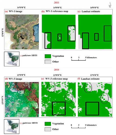
Figure 5.
Accuracy assessment vegetation proportion results from a randomly selected reference point. (a,d): WV-3 images in natural color composite. (b,e): The reference maps needed for validation. (c,f): Landsat vegetation proportion product. (i) and (ii): Are the locations of the selected reference points within our reference path/row. Circles and squares represent omission and commission errors for the vegetation proportion.
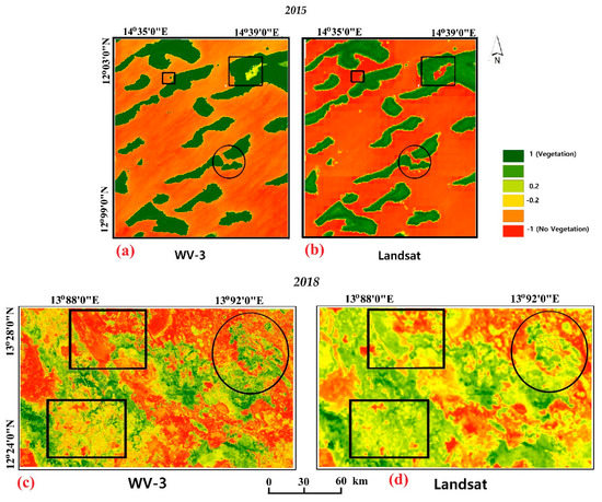
Figure 6.
Spatial comparison of vegetation proportion between the reference and Landsat products to visually demonstrate error rates. (a,c): Are WV-3 vegetation proportion composite images. (b,d): Are the vegetation proportion composite images derived from Landsat. The light green to dark green color represents vegetation pixels while the light red to dark red color represents non-vegetation pixels. Circles and squares represent some omission and commission errors respectively.
Table 4.
Results of accuracy validation for the vegetation proportion estimates.
Examples of the spatial differences between the reference maps and the vegetation proportion products from Landsat are shown in Figure 5. In each of the examples, we see that the disagreements are primarily located at the shaded areas in transitions between the vegetation and other land features. In such heterogeneous areas, vegetation proportions within the reference image were mapped out in a “patchy” manner (Figure 5e,f and Figure 6b).
The differences within the images indicates that the index slightly overestimated some areas that were or were not vegetation areas and could possibly explain the difference in the OA and kappa coefficient between the test periods. In areas where the distinction between vegetation and other land features area clear, this method can easily delineate vegetation proportions needed for VTCI model (Figure 5b,c and Figure 6a). Figure 5 and Figure 6 were provided to show visual examples of what Landsat error rates look like for individual vegetation proportion events.
4.2. VTCI Analysis
The warm and cold edges of each image were determined from their maximum and minimum LST products alongside their corresponding NDVI. These edges were crucial for the determination of VTCI for our study period. and obtained from a scatter plot of LST-NDVI for 2018/02/21 is shown in Figure 7. Similarly, the warm and cold edges for every composite image of LST and NDVI were obtained to calculate the VTCI during our study period. Table 5 shows the warm and cold edges for 2018, we see that the warm edge slopes were negative for that period. This indicates that decreases as NDVI increases for every NDVI interval. Contrary to the warm edge, the slopes of the cold edge were all positive indicating increases as NDVI increases. The shape of the scatter plot reveals our region of interest was large enough to provide numerous NDVI and LST estimates [48].
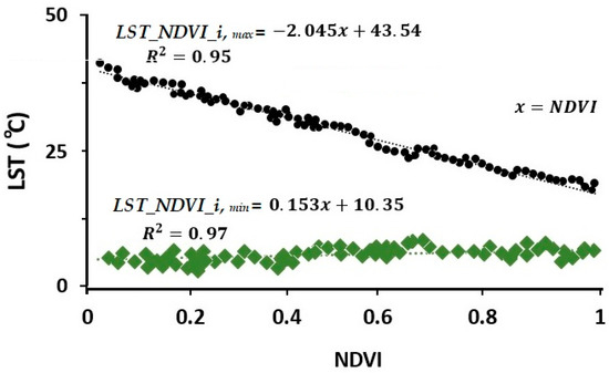
Figure 7.
Relationship between NDVI and LST for 2018/02/21.
Table 5.
NDVI-LST edges estimated by linear regression for 2018 during the peak dry season.
Figure 8 shows some results of the NDVI and LST obtained during the VTCI estimation process.
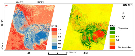
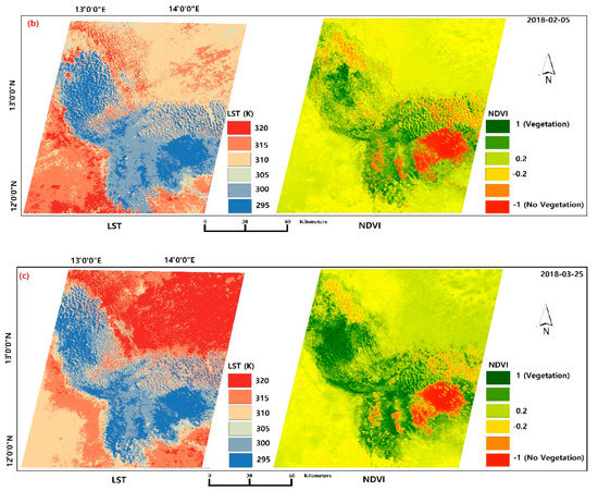
Figure 8.
Some LST and NDVI results for the path/row (185/51) for the year 2018.
The information obtained from the warm and cold edges for each composite image were used to calculate VTCI estimates during the study period. Figure 9 represents the averaged VTCI composites for the dry seasons of 1999, 2007, 2010, 2013, 2015, and 2018.
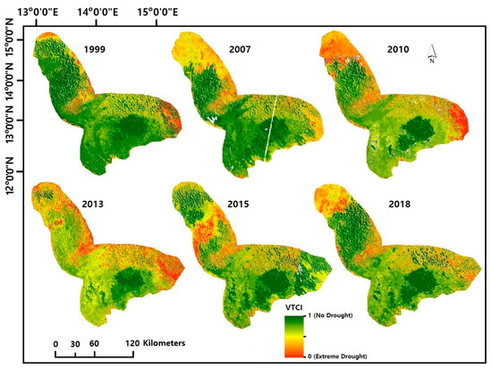
Figure 9.
Spatial distribution of averaged Vegetation Temperature Condition Index (VTCI) in Lake Chad between 1999 and 2018.
From these maps, we see that in 1999, there was very little drought that affected this region followed by a continuous decrease in moisture from 2007 to 2013 with most of the drought events occurring on the northern side of the lake. We also see that some drought (both extreme and severe conditions) creeping in from the south eastern section of that region. However, no prevailing extreme drought conditions are observed in the southern section of the lake. From 2015 to 2018, we see an improvement in the drought condition. However, an extreme drought situation prevailed in the northern section of the lake in 2018.
From Figure 9, we can see that sections or areas within the Lake Chad affected by different drought conditions varies over time. These variations can be examined with regard to temporal variations in the proportion of each drought category occurring over this area (Figure 10). We see from Figure 10 that most of the temporal variations occurred between three categories, moderate, severe and extreme drought. The No and Mild drought categories dominated our study area and together accounted for about 60% of the drought condition in this area. Meanwhile, the severe and extreme drought conditions fluctuated between 5% and 30%. Although No drought and Mild conditions dominated the entire area, we see a decrease in the Mild conditions by about 15% in 2013 and 2018. Though the No drought condition slightly increased during that period, we see that this decrease in Mild drought conditions was accounted for by an increase in moderate and severe drought conditions. The area under moderate drought decreases notably from 1999 to 2010 and peaks into the 18% range where it stayed slightly fluctuating. Generally, we see that areas under severe and extreme drought conditions marginally increases during this period with the most severe drought conditions experienced in 2010, 2013 and 2018.
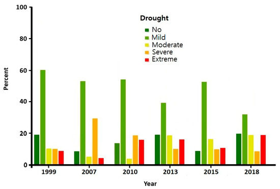
Figure 10.
Drought category changes for averaged VTCI in Lake Chad.
5. Discussion
VTCI, which is a combination of NDVI and LST both derived from Landsat images, was designed to characterize soil moisture conditions around Lake Chad. WV-3 images were used as reliable references for assessing the vegetation proportion derived from Landsat. Vegetation proportions extracted from Landsat were compared with those extracted from the reference data (WV-3) to verify the reliability of this method. An error matrix was used to obtain the overall accuracy, error of commission, error of omission and the kappa coefficient. The vegetation proportion products that were derived from the Landsat provided an accurate representation of the vegetation distribution and dynamics in this area. The corresponding validations relied on manual interpretation with calculated errors of commission and omission averaging 5.7% and 6.8%, respectively.
The spectral variability of vegetation depends on the canopy structure and biochemistry, like chlorophyll content. Visually inspecting Figure 5 and Figure 6, we see that different land feature types are assigned similar spectral signatures which may make extraction of specific features difficult. Generally, the accuracy of the vegetation proportion maps depends on the heterogeneous characteristic of the area mapped. When over an area where the land surface features can be easily distinguished, the overall accuracy of detecting vegetation proportion can exceed 95%. As it expands into environment of varying landforms, the accuracy decreases (Figure 6b,d).
Mixed pixel classifications are common in remote sensing practices. This is usually severe in areas where there is a mixture or transition between the different land surface features. In Figure 5f, the high amount of omission error (11.8%) indicates an under-classification of the vegetation proportion within that cell. These errors typically occurred along swamps or transition zones where the presence of both vegetation and non-vegetation features within the pixel led to a failure to identify vegetation (Figure 5e,f and Figure 6b). This can be further improved by applying sub-pixel and super-resolution mapping methods [48,49]. However, we minimized the use of selected reference products from such transition zones. Additionally, we assumed that the effect of the timing difference between the images used for accuracy assessment was negligible in regards to changes in vegetation proportion. The differences between vegetation proportion products seen in Figure 5 and Figure 6 could also be due to environmental factors, Landsat and WV-3 sensor, and processing differences which may result in differing spectral reflectance values for individual pixels.
The Lake Chad Basin has experienced a stable precipitation regime since the late 1990s, and despite these promising precipitation regimes, the discharge of the Chari River remained relatively low. It has also been reported that for equal precipitation, the Chari supplies approximately 30% as inflow into the southern pool of the lake [50]. The northern pool is known to be flooded during extreme wet conditions during which some of its inflow comes from the southern pool. In cases where discharge from the Chari River is low, overflow into the northern pool is not possible, which may explain why majority of the drought affects from that section of the lake (Figure 9). The drought pattern in the northern pool is to some extent consistent with those reported in a study from Lemoalle et al. [51], where the authors reported draw down surface areas in the northern pool of the lake varies from 0 to 2700 km2 depending on the Chari river discharge. However, water maps for this area show that the lake’s northern pool has been partially flooded every year since the early 2000s, without completely drying up [26]. This “positive” situation should allow for a better drought condition in the future given insecurity in this area has caused some inhabitants to move away, disrupting the relationship between the lake and the population [50]. Figure 9 also shows that some drought cases identified within the study period were not severe. This was further illustrated by the temporal variation of the drought categories in Figure 9. However, in an area like this where agricultural practices predominantly depend on the lake, such drought cases could be significant enough to negatively impact the food security conditions within the community. We also see in Figure 9 that over the years, major changes in the vegetation proportions in this area mostly occurred in the northern side of the lake. This is probably because the climate (Saharan desert climate) in this section is hot and dry, with rainfall ranging from 20–150 mm and temperatures greater than 35 °C. Contrarily, in the southern section of the lake, we see few changes in the vegetation proportion in that area. This is most likely because it is situated in the Sahel region with marked regional and seasonal variations in rainfall.
Lake Chad is known to have suffered a huge decline in freshwater availability mostly due to irrigation schemes, rainfall variability, extreme drought conditions and human activities [37,38,39]. LST and NDVI retrieved from Landsat data, may provide more valuable information about the temperature and vegetation health in this area (Figure 8). When combined, LST and NDVI can serve as a drought monitoring indicator. However, the different resolutions of NDVI and LST and usage of diverse sensors may affect the VTCI quality. For example, the 120 m resolution from the thermal band 6 of Landsat 5 may include mixtures of sand dunes, marshes and natural land forms peculiar for this area. These landforms may present abnormally high temperatures which could affect the magnitude and convergence of the cold and warm edges of the LST-NDVI space. In addition, the high dependence of image quality on the climatic environment is a possible drawback. Given the size of this area and its limited environmental data monitoring infrastructure, it is difficult obtaining ground observation data. This hinders the direct estimation of drought in this area. As such, the drought estimates from this study could not be evaluated against in situ drought estimates. A thorough validation exercise is needed by comparing VTCI values with in-situ measured soil moisture data if available. As the objective of this paper is to characterize drought patterns using VTCI from Landsat satellite, this has been designated as future work.
Ideally, all cloud free Landsat images would detect drought patterns within the Lake Chad Basin. Nevertheless, with a 16-day revisit period, Landsat satellites can only partially capture drought patterns for a given month. At such a temporal resolution, some flooding or drought events may be missed. However, it is still certain that the proposed approach analyzed by Landsat can be effectively used as a framework for long-term drought monitoring in this area. To enable a quick response to any drought situation, short time lags are required between data acquisition and information release. Therefore, given the 16-day revisit period of Landsat and cloud defects on some images, the seasonal drought patterns in this study have some limitations in real time processing of the Landsat data for drought monitoring.
Nonetheless, updates and development of new remote sensing technologies with higher temporal and spatial resolutions could serve as potential data sources for drought monitoring with higher precision. It is important to note that vegetation makes up over 50% of this area [24]. As seen in Figure 5 and Figure 6, this method has potential to accurately delineate vegetation patterns and health even in some transition area. This could serve as drought indicators for this area. During the calculation of vegetation proportion from the images used in this study, we did not use a uniform value to represent the maximum and minimum NDVI values. Instead, we carried out thorough visual inspection on each NDVI composite image to extract their respective minimum and maximum NDVI values which were later used to calculate their vegetation proportion. Though time consuming, it reduced the misclassification of some vegetation pixels. This process further reduced uncertainties associated with our method. It is advisable to exercise and observe such level of caution from data collection to result interpretation especially when dealing in areas with limited in-situ data. While policies for proper management of the lake are being put in place by the LCBC to ensure sustainable management of this water resource, we suggest that the influences of atmosphere and other additional channels on drought in this area should be investigated over a longer period. This can be achieved in future studies by cautiously incorporating recent datasets from ground observations, high resolution satellite data, and hydrological models.
6. Conclusions
The objective of this research was to characterize spatial drought patterns around the immediate environment of the Lake Chad. The VTCI derived from LST and NDVI in Landsat products is applied for the first time to monitor drought patterns in this area. We show examples for the identification of extreme events to demonstrate the ability of Landsat products to capture and represent spatial and temporal details. A Vegetation Index, (NDVI) and Land Surface Temperature (LST) from Landsat were used as indicators for drought monitoring. Using the outputs from LST and NDVI, Vegetation Temperature Condition Index (VTCI) composites were derived. Analyses of averaged VTCI estimates obtained during the study period revealed a high drought occurrence in the northern section of the Lake area.
Landsat data were used for these analyses and as shown, had some limitations in terms of resolutions where we had some pixels being reported as vegetation which were false. In addition to that limitation, Landsat images are also limited by cloudiness which reduces the amount of data available at a given time. However, for this study we were able to find suitable cloudless images from Landsat for our analyses. Issues related to misjudgment of features due to image resolution can be addressed through the use of very high-resolution images. With further result testing and the consistent availability of cloud free multispectral images, this approach has the potential to provide a general framework for future drought monitoring, thermal conditions and vegetation health in this area.
According to the VTCI series shown in Figure 7, despite the severe drought conditions experienced in the dry seasons of 2007 and 2010, we see a significant improvement in 2013. Compared to previous studies, this work provides a simple and efficient way of addressing the issue of drought in this area. The findings of this study can assist and support improved sustainable management policies especially in the UNESCO’s BIOsphere and Heritage of Lake Chad (BIOPALT) project which aims at producing early warning systems for drought.
Author Contributions
W.G.B. and S.-I.L. developed the methodology and the manuscript. W.G.B. conducted the work with technical assistance from S.-I.L.
Funding
This subject is supported by Korea Environment Industry & Technology Institute (KEITI) through Water Management Research Program, funded by Korea Ministry of Environment (MOE; 79623), and also supported by Basic Science Research Program through the National Research Foundation of Korea (NRF) funded by the ministry grant (NRF-2018R1D1A1A09083120).
Acknowledgments
The authors would like to thank the reviewers and editors for their valuable comments and suggestions.
Conflicts of Interest
The authors declare no conflict of interest.
References
- Bordi, I.; Sutera, A. Drought Monitoring and Forecasting at Large Scale. In Methods and Tools for Drought Analysis and Management; Rossi, G., Vega, T., Bonaccorso, B., Eds.; Springer: Dordrecht, The Netherlands, 2007; Volume 62. [Google Scholar] [CrossRef]
- Bond, N.R.; Lake, P.S.; Arthington, A.H. The impacts of drought on freshwater ecosystems: An Australian perspective. Hydrobiologia 2008, 600, 3–16. [Google Scholar] [CrossRef]
- Masih, I.; Maskey, S.; Mussá, F.E.F.; Trambauer, P. A review of droughts on the African continent: A geospatial and long-term perspective. Hydrol. Earth Syst. Sci. 2014, 18, 3635–3649. [Google Scholar] [CrossRef]
- Bijaber, N.; El Hadani, D.; Saidi, M.; Svoboda, M.; Wardlow, B.; Hain, C.; Poulsen, C.; Yessef, M.; Rochdi, A. Developing a remotely sensed drought monitoring indicator for morocco. Geosciences 2018, 8, 55. [Google Scholar] [CrossRef]
- Zeng, L.; Shan, J.; Xiang, D. Monitoring drought using multi-sensor remote sensing data in cropland of Gansu Province. In IOP Conference Series: Earth and Environmental Science; IOP Publishing: Bristol, UK, 2014; Volume 17. [Google Scholar] [CrossRef]
- Villarreal, M.L.; Norman, L.M.; Buckley, S.; Wallace, C.S.A.; Coe, M.A. Multi-index time series monitoring of drought and fire effects on desert grasslands. Remote Sens. Environ. 2016, 183, 186–197. [Google Scholar] [CrossRef]
- AghaKouchak, A.; Farahmand, A.; Melton, F.S.; Teixeira, J.; Anderson, M.C.; Wardlow, B.D.; Hain, C.R. Remote sensing of drought: Progress, challenges and opportunities. Rev. Geophys. 2015, 53, 452–480. [Google Scholar] [CrossRef]
- Liu, X.; Zhu, X.; Pan, Y.; Li, S.; Liu, Y.; Ma, Y. Agricultural drought monitoring: Progress, challenges, and prospects. J. Geogr. Sci. 2016, 26, 750–767. [Google Scholar] [CrossRef]
- Palmer, W.C. Meteorological Drought; Research Paper No. 45; U.S. Weather Bureau: Washington, DC, USA, 1965.
- Mckee, T.B.; Doesken, N.J.; Kleist, J. The relationship of drought frequency and duration to time scales. In Proceedings of the Eighth Conference on Applied Climatology, Anaheim, CA, USA, 17–22 January 1993; pp. 179–184. [Google Scholar]
- Zhao, M.; Velicogna, I.; Kimball, J.S. Satellite observations of regional drought severity in the continental United States using GRACE-based terrestrial water storage changes. J. Clim. 2017, 30, 6297–6308. [Google Scholar] [CrossRef]
- Qian, X.; Liang, L.; Shen, Q.; Sun, Q.; Zhang, L.; Liu, Z.; Zhao, S.; Qin, Z. Drought trends based on the VCI and its correlation with climate factors in the agricultural areas of China from 1982 to 2010. Environ. Monit. Assess. 2016, 188, 939. [Google Scholar] [CrossRef]
- Kogan, F.N. Application of vegetation index and brightness temperature for drought detection. Ad. Space Res. 1995, 15, 91–100. [Google Scholar] [CrossRef]
- Unganai, L.S.; Kogan, F.N. Drought monitoring and corn yield estimation in southern Africa from AVHRR data. Remote Sens. Environ. 1998, 63, 219–232. [Google Scholar] [CrossRef]
- Nazla, B.; Robert, V.R.; Nina, S.N.L.; Lei, Z.; Rubayet, B.M.; Volodymyr, M. The relationship between the Normalized Difference Vegetation Index and drought indices in the South Central United States. Nat. Hazards 2019, 96, 791–808. [Google Scholar] [CrossRef]
- Davenport, M.L.; Nicholson, S.E. On the relation between rainfall and the normalized difference vegetation index for diverse vegetation types in east Africa. Int. J. Remote Sens. 1993, 14, 2369–2389. [Google Scholar] [CrossRef]
- Rouse, J.W.; Haas, R.H.; Schell, J.A.; Deering, D.W. Monitoring Vegetation Systems in the Great Plains with ERTS (Earth Resources Technology Satellite). In Proceedings of the Third Earth Resources Technology Satellite Symposium, Greenbelt, ON, Canada, 10–14 December 1973; Volume SP-351, pp. 309–317. [Google Scholar]
- Tucker, C.J. Red and photographic infrared linear combinations for monitoring vegetation. Remote Sens. Environ. 1979, 8, 127–150. [Google Scholar] [CrossRef]
- Chen, D.; Brutsaert, W. Satellite-sensed distribution and spatial patterns of vegetation parameters over a tallgrass prairie. J. Atmos. Sci. 1998, 55, 1225–1238. [Google Scholar] [CrossRef]
- Nanzad, L.; Zhang, J.; Tuvdendorj, B.; Nabil, M.; Zhang, S.; Bai, Y. NDVI anomaly for drought monitoring and its correlation with climate factors over Mongolia from 2000 to 2016. J. Arid Environ. 2019, 164, 66–77. [Google Scholar] [CrossRef]
- Liu, L.; Yang, X.; Zhou, H.; Liu, C.; Zhou, L.; Li, X.; Yang, J.; Han, X.; Wu, J. Evaluating the utility of solar-induced chlorophyll fluorescence for drought monitoring by comparison with NDVI derived from wheat canopy. Sci. Total Environ. 2017, 625, 1208–1217. [Google Scholar] [CrossRef]
- Orhan, O.; Ekercin, S.; Dadaser-Celik, F. Use of Landsat land surface temperature and vegetation indices for monitoring drought in the salt lake basin area, Turkey. Sci. World J. 2014, 2014, 11. [Google Scholar] [CrossRef]
- Ghaleb, F.; Mario, M.; Sandra, N.A. Regional Landsat-Based Drought Monitoring from 1982 to 2014. Climate 2015, 3, 563–577. [Google Scholar] [CrossRef]
- Buma, W.G.; Lee, S.I.; Seo, J.Y. Recent surface water extent of Lake Chad from multispectral sensors and grace. Sensors 2018, 18, 2082. [Google Scholar] [CrossRef]
- Boronina, A.; Ramillien, G. Application of AVGRR imagery and GRACE measurements for calculation of actual evapotranspiration over the Quaternary aquifer (Lake Chad basin) and validation of groundwater models. Hydrol. J. 2008, 348, 98–109. [Google Scholar] [CrossRef]
- Adeyeri, O.E.; Lamptey, B.L.; Lawin, A.E.; Sanda, I.S. Spatio-temporal precipitation trend and homogeneity analysis in Komadugu-Yobe basin, Lake Chad region. J. Climatol. Weather Forecast. 2017, 5, 12. [Google Scholar] [CrossRef]
- Gao, H.; Bohn, T.J.; Podest, E.; McDonald, K.C.; Lettenmaier, D.P. On the causes of the shrinking of Lake Chad. Environ. Res. Lett. 2011, 6, 034021. [Google Scholar] [CrossRef]
- Coe, M.T.; Foley, J.A. Human and natural impacts on the water resources of the Lake. Geophys. Res. Atmos. 2001, 106, 3349–3356. [Google Scholar] [CrossRef]
- Coe, M.T.; Birkett, C.M. Calculation of river discharge and prediction of lake height from satellite radar altimetry: Example for the Lake Chad basin. Water Resour. Res. 2004, 40. [Google Scholar] [CrossRef]
- Nkiaka, E.; Nawaz, N.R.; Lovett, J.C. Using standardized indicators to analyse dry/wet conditions and their application for monitoring drought/floods: A study in the Logone catchment, Lake Chad basin. Hydrol. Sci. J. 2017, 62, 2720–2736. [Google Scholar] [CrossRef]
- Ndehedehe, C.E.; Agutu, N.O.; Okwuashi, O.; Ferreira, V.G. Spatio-temporal variability of droughts and terrestrial water storage over lake chad basin using independent component analysis. J. Hydrol. 2016, 540, 106–128. [Google Scholar] [CrossRef]
- Okonkwo, C.; Demoz, B.; Onyeukwu, K. Characteristics of drought indices and rainfall in Lake Chad Basin. Int. J. Remote Sens. 2013, 34, 7945–7961. [Google Scholar] [CrossRef]
- United Nations Educational, Scientific and Cultural Organization (UNESCO). BIOsphere and Heritage of Lake Chad (BIOPALT) Project. 2018. Available online: https://en.unesco.org/biopalt (accessed on 29 October 2019).
- Leblanc, M.; Lemoalle, J.; Bader, J.-C.; Tweed, S.; Mofor, L. Thermal remote sensing of water under flooded vegetation: New observations of inundation patterns for the ‘Small’ Lake Chad. J. Hydrol. 2011, 404, 87–98. [Google Scholar] [CrossRef]
- Buma, W.G.; Lee, S.I.; Seo, J.Y. Hydrological evaluation of Lake Chad Basin using space borne and hydrological model observations. Water 2016, 8, 205. [Google Scholar] [CrossRef]
- Lemoalle, J. Lake Chad: A Changing Environment. In Dying and Dead Seas Climatic Versus Anthropic Causes; NATO Science Series: IV: Earth and Environmental Sciences; Nihoul, J.C.J., Zavialov, P.O., Micklin, P.P., Eds.; Springer: Dordrecht, The Netherlands, 2004; Volume 36. [Google Scholar] [CrossRef]
- Lake Chad Basin Commission (LCBC). The Lake Chad Basin. 2014. Available online: http://www.cblt.org/en/lake-chad-basin (accessed on 29 October 2019).
- Feyisa, G.L.; Meilby, H.; Fensholt, R.; Proud, S.R. Automated Water Extraction Index: A New Technique for Surface Water Mapping Using Landsat Imagery. Remote Sens. Environ. 2014, 140, 23–35. [Google Scholar] [CrossRef]
- Yang, J.; Du, X. An enhanced water index in extracting water bodies from Landsat TM imagery. Ann. GIS 2017, 23, 141–148. [Google Scholar] [CrossRef]
- Chen, J.; Zhu, X.L.; Vogelmann, J.E.; Gao, F.; Jin, S.M. A simple and effective method for filling gaps in Landsat ETM plus SLC-off images. Remote Sens. Environ. 2011, 115, 1053–1064. [Google Scholar] [CrossRef]
- Dash, P.; Göttsche, F.M.; Olesen, F.S.; Fischer, H. Land surface temperature and emissivity estimation from passive sensor data: Theory and practice-current trends. Int. J. Remote Sens. 2002, 23, 2563–2594. [Google Scholar] [CrossRef]
- Sobrino, J.A.; Jiménez-Muñoza, J.C.; Paolinib, L. Land surface temperature retrieval from LANDSAT TM 5. Remote Sens. Environ. 2004, 90, 434–440. [Google Scholar] [CrossRef]
- Sobrino, J.A.; Caselles, V.; Becker, F. Significance of the remotely sensed thermal infrared measurements obtained over a citrus orchard. ISPR J. Photogramm. 1990, 44, 343–354. [Google Scholar] [CrossRef]
- Wang, P.X.; Li, X.W.; Gong, J.Y.; Song, C.H. Vegetation temperature condition index and its application for drought monitoring. In Proceedings of the International Geoscience and Remote Sensing Symposium, Sydney, Australia, 9–13 July 2001; pp. 141–143. [Google Scholar] [CrossRef]
- Mühlbauer, S.; Costa, A.C.; Caetano, M. A spatiotemporal analysis of droughts and the influence of North Atlantic oscillation in the Iberian Peninsula based on MODIS imagery. Theor. Appl. Climatol. 2016, 124, 703–721. [Google Scholar] [CrossRef]
- Marc, P.; Stephen, V.S.; Emilio, C. Validation of the 2008 MODIS-MCD45 global burned area product using stratified random sampling. Remote Sens. Environ. 2014, 144, 187–196. [Google Scholar] [CrossRef]
- Olofsson, P.; Foody, G.M.; Stehman, S.V.; Woodcock, C.E. Making better use of accuracy data in land change studies: Estimating accuracy and area and quantifying uncertainty using stratified estimation. Remote Sens. Environ. 2013, 129, 122–131. [Google Scholar] [CrossRef]
- Gillies, R.R.; Carlson, T.N.; Cui, J.; Kustas, W.P.; Humes, K.S. A verification of the ‘triangle’ method for obtaining surface soil water content and energy fluxes from remote measurement of the Normalized Difference Vegetation Index (NDVI) and surface radiant temperature. Int. J. Remote Sens. 1997, 18, 3145–3166. [Google Scholar] [CrossRef]
- Xu, H. Modification of normalised difference water index (NDWI) to enhance open water features in remotely sensed imagery. Int. J. Remote Sens. 2007, 27, 3025–3033. [Google Scholar] [CrossRef]
- Agence Française de Developpement. Available online: https://www.afd.fr/fr/lac-tchad-boko-haram?origin=/fr/ressources-a=1 (accessed on 29 October 2019).
- Lemoalle, J.; Bader, J.-C.; Leblanc, M.; Sedick, A. Recent changes in Lake Chad: Observations, simulations and management options (1973–2011). Glob. Planet. Chang. 2012, 8081, 247–254. [Google Scholar] [CrossRef]


© 2019 by the authors. Licensee MDPI, Basel, Switzerland. This article is an open access article distributed under the terms and conditions of the Creative Commons Attribution (CC BY) license (http://creativecommons.org/licenses/by/4.0/).