


Abstract
Accurate solar power forecasting is a key technology for efficient operation of photovoltaic (PV) power plants and safe grid dispatch. Under the “dual carbon” goals and the increasing share of renewable energy connected to the grid, ultra-short-term power forecasting is important for improving dispatch decisions and supporting system operation. To address the ultra-short-term forecasting task at two PV sites, this study develops an end-to-end framework that integrates machine learning, Bayesian optimisation, and SHAP-based interpretability. First, correlation analysis was performed on the datasets from the two sites to provide a foundation for subsequent model development. Next, seven forecasting models, including CatBoost, NGBoost, Random Forest (RF), AdaBoost, ARIMA, CNN-LSTM, and LSTM, were developed and uniformly optimised using Bayesian optimisation. Under a unified framework of data partitioning, optimisation budget, and evaluation metrics, the predictive performance of all models at the two sites was systematically assessed. The results show that the optimal model varies across sites: at Site 1, LSTM delivered the best performance, with test-set R2, MSE, RMSE, and MAE values of 0.972, 17.610, 4.196, and 2.267, respectively; at Site 2, CatBoost achieved the best results, with corresponding values of 0.994, 0.385, 0.621, and 0.249, respectively. These findings highlight pronounced site-specific differences in model performance, indicating that different modeling approaches exhibit distinct adaptability under varying data characteristics and operational conditions. Further error analysis and SHAP interpretation indicate that solar irradiation and key meteorological variables are the main drivers of power output, and their effects are nonlinear, confirming the model’s ability to capture complex nonlinear relationships in PV power forecasting. Finally, a graphical user interface (GUI) tool was developed to support site selection, real-time forecasting, and parameter input, providing a practical and convenient solution for PV plant operation and grid dispatch.
1. Introduction
Against the global move toward a low-carbon energy system and the increasing share of renewable energy connected to the grid, solar power has become an important source of new generation capacity because it is clean, widely available, and easy to scale up [1]. At the same time, power systems require better predictability and controllability of solar generation due to issues such as cross-regional power transfer and the need to improve system resilience [2]. However, solar power output is highly sensitive to changes in solar irradiance and cloud movement. Large short-term fluctuations can lead to higher reserve requirements, more frequent charging and discharging of energy storage, and a higher risk of curtailment, which reduces grid safety margins and worsens operating costs [3,4,5,6,7]. Therefore, to meet the needs of rolling dispatch and real-time control, high accuracy photovoltaic (PV) power forecasting at minute to hour time scales is necessary. In particular, 15-min-ahead ultra-short-term point forecasting fits the practical requirements of rolling dispatch and short-term control [8,9], and it has become a key technology for improving renewable energy integration and dispatch performance [10]. More accurate ultra-short-term photovoltaic power forecasting not only allows short-timescale power fluctuations to be characterised more precisely, thereby supporting rolling dispatch, real-time control, and reserve capacity allocation, but also provides more reliable information for renewable energy accommodation and grid integration. Therefore, this study is of considerable practical significance.
Solar power forecasting methods have developed over time, from physics-based models [11] and numerical weather prediction (NWP)-driven approaches, to statistical time series models [12], and then to data-driven machine learning methods. Many review studies report that machine learning and ensemble learning are effective in learning the nonlinear relationship between meteorological variables and solar power output, and they can better handle uncertainty from multiple sources [13,14]. In addition, probabilistic forecasting and uncertainty quantification have become important research topics in this field [15]. For short-term solar forecasting, studies have explored regional scale prediction, irradiance learning models, and distributed probabilistic forecasting [16]. Some works also proposed irradiance prediction based on random learning and multi-source observation fusion [17]. Other studies evaluated the feasibility and limits of forecasting that relies only on historical power data, without exogenous inputs [18]. Deep learning has further improved feature representation in complex situations [19,20,21]. Even so, model selection, hyperparameter settings, and cross-site reproducibility are still key factors that affect the reliability of conclusions and limit engineering deployment [22,23,24].
Recent dedicated reviews on solar power forecasting have shown that research in this field has gradually expanded from conventional single-model point forecasting to multi-timescale forecasting, probabilistic forecasting, hybrid modeling, real-time data fusion, and grid-oriented applications. Especially for ultra-short-term to short-term forecasting, input feature construction, temporal resolution, forecast horizon setting, model generalisation, and uncertainty characterization have been recognized as key factors affecting prediction accuracy and reliability. Therefore, systematic comparisons of different models under a unified experimental protocol, while jointly considering accuracy, robustness, and interpretability, remain of clear research value.
From the perspective of practical modeling, several machine learning methods have been widely used and provide a solid basis for architecture design, optimisation, and interpretability. Random Forest (RF), a typical bagging ensemble method, uses multiple trees and averaging to reduce variance, and it is often used in prediction tasks with noisy data and correlated features. Boosting methods improve weak learners step by step and focus more on hard samples, which makes them effective for building high- accuracy regressors. For tabular data, Categorical Boosting (CatBoost) reduces bias and improves generalisation through ordered boosting and related techniques, providing an efficient solution for mapping meteorological inputs to power output. In addition, probabilistic boosting frameworks extend point forecasts to predictive distributions, which supports uncertainty quantification [25].
Although machine learning-based solar forecasting has made clear progress, three main problems still limit engineering implementation and wider use. First, model comparison is often not systematic enough. Without unified benchmarking across models and consistent evaluation across sites, performance results can be strongly affected by data splitting and evaluation settings, making it difficult to identify the best model for different scenarios. Second, hyperparameter optimisation remains challenging [26]. Forecast accuracy is sensitive to the optimisation method, but efficient strategies are still not fully used in multi model systems. Traditional approaches are often slow and can get stuck in local optima, which reduces fairness in comparison and prevents models from reaching their best performance [27]. Third, interpretability is still insufficient. Many forecasting models behave like black boxes and do not provide clear and traceable explanations for their predictions, so dispatchers cannot easily understand key factor contributions or operational patterns [28,29]. In addition, many studies focus on offline experiments and do not offer interactive tools for dispatch and operation, which slows down the transfer of research results to practical use [30].
To address these issues, this study proposes a machine learning based framework for ultra-short-term solar power forecasting and interpretability analysis. The main contributions are as follows:
(1) An ultra-short-term forecasting framework is built using Random Forest (RF), Natural Gradient Boosting (NGBoost), CatBoost, Adaptive Boosting (AdaBoost), Autoregressive Integrated Moving Average (ARIMA), Convolutional Neural Network–Long Short-Term Memory (CNN-LSTM), and Long Short-Term Memory (LSTM) to handle the requirements of 15-min-ahead PV power prediction.
(2) Bayesian optimisation is tightly integrated with the machine learning models to achieve efficient hyperparameter search and to improve prediction performance.
(3) A SHapley Additive exPlanations (SHAP)-based interpretability framework is established to analyse the prediction mechanism and improve transparency and credibility, and a graphical user interface (GUI) is developed to support fast evaluation and engineering deployment.
The remainder of this paper is organised as follows. Section 2 presents the overall technical framework for solar power forecasting. Section 3 describes the dataset, variable definitions, and data preprocessing. Section 4 introduces the methods, including machine learning models, Bayesian hyperparameter optimisation, and SHAP interpretability. Section 5 reports comparative experiments to verify the value of Bayesian optimisation, compares different models, provides interpretability results, and introduces the GUI tool and its deployment approach. Finally, Section 6 summarises the conclusions and discusses future work.
2. Overall Framework
As shown in Figure 1, this study develops a systematic framework for ultra-short-term solar power forecasting. Based on a meteorological feature system, the framework integrates model training, Bayesian hyperparameter optimisation, and interpretable analysis using modern machine learning methods, thereby forming a complete workflow from data processing to deployment with improved transparency. First, the datasets from Sites 1 and 2 are organised and the variables are standardised. For each site, correlation matrices are plotted to examine the statistical relationships between meteorological variables and power output, thereby providing a clear basis for model development. Next, seven representative models, including CatBoost, NGBoost, Random Forest, AdaBoost, ARIMA, CNN-LSTM, and LSTM, are developed for each site. Bayesian optimisation is applied to tune the hyperparameters of all models, leading to improved accuracy and generalisation under complex nonlinear conditions. Error diagnostics are then used to evaluate prediction consistency and bias patterns, confirming that the model outputs are stable and suitable for practical applications.
Figure 1.
Overall Framework.
To ensure a fair comparison among models and enhance the reliability of the results, a rigorous time-series splitting strategy together with a unified evaluation framework is further adopted in this study. All samples are chronologically divided into sub-training, validation, and test sets, and Bayesian optimisation coupled with TimeSeriesSplit is performed on the sub-training set to effectively prevent future information leakage. Under a unified protocol in terms of data partitioning, optimisation budget, and evaluation metrics, the predictive performance of different models at the two sites is comprehensively assessed. Furthermore, the Diebold–Mariano (DM) test is employed to verify the statistical significance of performance differences among models, thereby providing a robust foundation for the subsequent SHAP-based interpretability analysis and GUI-oriented engineering deployment of the selected optimal models. Finally, SHAP analysis is performed on the site-specific optimal model to identify the key contributions of variables such as solar irradiation and other meteorological factors to power prediction. This improves the credibility of the results and provides quantitative evidence for dispatch and operation. The selected model is further packaged into an interactive GUI tool that supports site selection, input parameter settings, and real-time power forecasting, thereby completing a closed-loop process covering modeling, optimisation, error analysis, interpretation, and engineering delivery.
3. Dataset
This study uses the publicly released renewable energy generation dataset from the State Grid Corporation of China and focuses on modeling and comparative analysis for two solar power stations. The data cover the period from 2019 to 2020 with a 15-min sampling interval, which support ultra-short-term point forecasting for the next time step, that is, 15 min ahead. The two sites show clear differences in plant scale and output level, and the overall average actual power output mainly falls within the range of 0 to 50 MW.
The forecasting target in this paper is the site-level actual output power (Power, MW), and the task is formulated as single-step ultra-short-term forecasting. The input variables include solar irradiance and meteorological conditions. The irradiance variables are total solar irradiance (TSI), direct normal irradiance (DNI), and global horizontal irradiance (GHI). The meteorological variables include air temperature (Air_T) and air pressure (Air_P), and some sites also include relative humidity (Air_H). For Site 1 and Site 2, six input features are used: TSI, DNI, GHI, Air_T, Air_P, and Air_H. To keep the variable meaning, units, and engineering context clear and traceable, the definitions and units of all input and output variables are summarised in Table 1.
Table 1.
Solar Power Station Data Field Definitions.
3.1. Dataset Correlation Analysis
Correlation analysis was carried out for Site 1 to examine the relationships between the input variables and power output. The PV output power shows the highest correlation with TSI and also has strong positive correlations with DNI and GHI, indicating that irradiance changes are the main driver of short-term power fluctuations at this site. In comparison, Air_T shows a moderate positive correlation with power output, Air_P shows a weak and slightly negative correlation, and Air_H shows a clear negative correlation. This suggests that higher humidity may be linked to stronger cloud effects or increased scattering, which reduces effective irradiance and leads to lower power generation. In addition, TSI, DNI, and GHI are highly correlated with each other, and Air_T and Air_P show a strong negative correlation, which indicates possible multicollinearity among the inputs. The Pearson correlation coefficient matrix is presented in Figure 2.
Figure 2.
Correlation Matrix for Site 1 Dataset.
This study also examined the correlation between the input variables and power output at Site 2. The results show strong positive correlations between PV power and irradiance variables (TSI, DNI, and GHI). In particular, TSI has a correlation coefficient of 0.99, indicating that irradiance changes have the largest impact on short-term power fluctuations. Air temperature (Air_T) shows a moderate to strong positive correlation with power output, while air humidity (Air_H) shows a clear negative correlation, suggesting that higher humidity is associated with lower power generation. In contrast, the correlation between atmospheric pressure (Air_P) and power output is close to zero, which indicates a limited influence. In addition, the irradiance variables are highly correlated with each other, for example, the correlation coefficient between TSI and DNI is 0.95, and Air_T has a strong negative correlation with Air_P. These patterns suggest possible multicollinearity among the input variables. The Pearson correlation coefficient matrix is shown in Figure 3.
Figure 3.
Correlation Matrix for Site 2 Dataset.
To further evaluate multicollinearity among the input variables, the variance inflation factor (VIF) values of the major meteorological features at the two sites were calculated, as summarized in Table 2. Several features at both sites exhibited relatively high VIF values, particularly TSI and DNI, while GHI also showed a high VIF value at Site 1, indicating substantial linear dependence and redundancy among the irradiance-related variables. Therefore, the SHAP importance rankings of these variables should be interpreted cautiously, as they more likely reflect the dominant contribution of the irradiance feature group as a whole rather than strictly independent physical effects of individual variables.
Table 2.
Variance inflation factor (VIF) results for the main input variables at the two sites.
3.2. Data Preprocessing and Time-Series Splitting Strategy
Solar power forecasting is inherently a time-series problem characterised by significant temporal autocorrelation among samples. Therefore, data preprocessing and partitioning were executed strictly in chronological order prior to modeling. Initially, the column names of the raw data were standardised, and the temporal and target variables were identified, with time fields converted into a standard timestamp format. Unparseable temporal records were discarded, and duplicate timestamps were removed. Subsequently, all valid samples were sorted in ascending chronological order to ensure strict temporal sequence across the subsequent training, validation, and testing phases. Originally, both Site 1 and Site 2 contained 70,176 raw observations. After preprocessing, 52,119 and 70,174 valid samples were retained for Site 1 and Site 2, respectively. The exclusion of samples primarily resulted from the removal of negative power values and the truncation of initial invalid records generated during lag feature construction. A summary of the valid observations used for modeling and the corresponding sample exclusions after data cleaning and preprocessing is presented in Table 3.
Table 3.
Dataset filtering and valid sample retention across different sites.
Regarding feature engineering for supervised learning-based forecasting models, this study utilised raw meteorological variables as foundational inputs, further augmented by temporal and lag features. Specifically, basic temporal features—including month, day, hour, minute, and day of the week—were extracted to capture the cyclical patterns of solar power generation. Concurrently, lag features of both the target variable and meteorological variables were constructed to enhance the models’ capacity to represent ultra-short-term dynamic variations. Missing values inevitably generated at the beginning of the sequence due to the lag operation were handled by truncating the initial few invalid samples. For any remaining missing input values, a median imputation strategy fitted solely on the training data was employed during the modeling phase. To strictly prevent data leakage, this imputation process was embedded within the respective pipelines or internal architectures of the different models, in accordance with their specific algorithmic frameworks. Conversely, for classical statistical time-series models, the standard input format of modeling based purely on historical power sequences was retained.
To ensure the rigor of the experimental evaluation, a unified, three-stage chronological splitting strategy was applied to all models. Initially, the first 80% of the samples were allocated as the training-development set, while the remaining 20% were reserved as the testing set. Within the training-development set, the chronological last 10% of samples were further designated as the validation set, leaving the remainder as the sub-training set. Consequently, the sub-training, validation, and testing sets progress sequentially in time without any overlapping. Although all models were compared under this unified chronological splitting and evaluation framework, the specific preprocessing methods and input construction formats required by different algorithms were preserved. This ensures that the comparative analysis is not only fair and consistent but also conforms to the fundamental mechanisms of the various models.
Given the significant temporal autocorrelation among time-series samples, traditional randomized k-fold cross-validation could lead to future information leakage. Therefore, a time-series-aware TimeSeriesSplit strategy was uniformly adopted during the hyperparameter optimisation process. Specifically, Bayesian optimisation searches for all models were conducted exclusively on the sub-training set in conjunction with TimeSeriesSplit. The validation set was excluded from the parameter search and utilised solely to evaluate the generalisation capability of the optimal hyperparameter configurations. Upon determining the optimal hyperparameters, each model was retrained on the entire training-development set, and the final predictive performance was reported based on the independent testing set. This strategy effectively circumvents future data leakage, thereby enhancing the reliability and reproducibility of the model evaluation results.
4. Methodology
4.1. Solar Power Generation Forecasting
Solar power forecasting is a nonlinear system modeling problem driven by high dimensional meteorological features. The goal is to build an accurate map from the environmental state to the power output. In real PV plants, the output is affected by coupled factors such as atmospheric radiative transfer, PV module photoelectric conversion, and grid side control. As a result, the power series often shows stochastic fluctuations and time varying nonstationary behaviour. Therefore, model performance depends not only on the fitting ability of the algorithm, but also on whether the selected input variables can properly describe the physical drivers and the main operational constraints.
In general, the instantaneous output power of a PV array can be described as a function of solar irradiance input and the overall conversion efficiency. A general form is given by [31]:
where is the irradiance vector, including total solar irradiance, direct normal irradiance, and global horizontal irradiance, which determines the upper limit of energy input. is the thermal state, mainly ambient temperature, which affects the module junction temperature and then changes the open circuit voltage and conversion efficiency. represents other environmental conditions, such as relative humidity, atmospheric pressure, and aerosol related effects, which mainly influence atmospheric scattering and spectral attenuation. represents operational constraints, such as inverter maximum power point tracking efficiency, power limiting commands, and protection logic. Compared with simplified physics-based models that use irradiance and temperature only, this study adopts the above general mapping to better cover nonlinear responses, nonstationary behaviour, and control effects in practical sites.
In real operation, measurement noise and system uncertainties are unavoidable, and prediction accuracy is usually limited by three related factors. First, irradiance and meteorological drivers dominate short-term changes. Irradiance variables set the upper bound of output, while changes in cloud cover and water vapour directly affect transmittance and are a major source of short-term errors. Temperature, pressure, and humidity further influence the response through cell operating temperature and atmospheric attenuation. Second, site and environmental differences can cause large performance gaps across stations, including terrain and shading, module tilt and azimuth, dust and pollution, and seasonal changes in solar altitude. Third, equipment and operational constraints introduce deviations from the ideal irradiance to power relationship, such as module ageing, mismatch, inverter control strategy, grid connection limits, and maintenance events, which can create structural bias in some periods. From an application view, PV power forecasting can be classified by time scale into ultra-short-term, short-term, medium term, and long term, each serving different decisions. This paper focuses on ultra-short-term point forecasting for 15 min ahead, and uses machine learning to learn the mapping from irradiance and meteorological inputs to power output based on site data, providing more reliable support for dispatch and operation management.
4.2. Machine Learning Models
4.2.1. CatBoost Model
CatBoost is an improved algorithm built on the Gradient Boosting Decision Tree (GBDT) framework. By using symmetric tree structures and an ordered boosting strategy, it can reduce prediction bias and lower the risk of overfitting compared with traditional GBDT methods.
For regression, suppose the model is updated at iteration . The prediction function can be written as a weighted update from the previous model and the current base learner [32]:
where is the cumulative prediction from the first iterations, is the regression tree trained at the -th iteration, and is the learning rate.
CatBoost trains the model by minimising the empirical risk with a regularisation term:
where is the loss function (mean squared error, MSE, in this study), and controls model complexity. At each iteration, the new base learner is fitted to the negative gradient of the loss, also called the pseudo residual. For sample , the pseudo residual at iteration is defined as
As a strong ensemble method, CatBoost can model the nonlinear relationship between meteorological inputs and PV power output. It is also robust when the input data are heterogeneous, which makes it suitable for practical solar power forecasting tasks.
4.2.2. NGBoost Model
NGBoost (Natural Gradient Boosting) is a probabilistic forecasting algorithm. Unlike traditional point-prediction models, it aims to estimate the conditional probability distribution of the target variable given an input . This simultaneously achieves point forecasting of power and uncertainty quantification .
Assuming the target variable follows a specific parameter distribution family (e.g., the normal distribution ), the model learns the distribution’s parameter vector through a boosting approach. During the th iteration, the parameter update formula is [33]
where is the base learner fitting the natural gradient.
The core of NGBoost lies in utilising natural gradients instead of conventional gradients for parameter updates, thereby adapting to the geometric structure of the probability distribution manifold. The objective function is to minimise the negative log-likelihood (NLL), specifically the proper scoring rule:
For a sample , its natural gradient with respect to parameters is defined as
where denotes the Fisher information matrix, which measures the statistical distance within the parameter space.
In the solar power forecasting task addressed herein, given the strong randomness of irradiance and meteorological data, NGBoost can provide confidence interval support for scheduling decisions by outputting distribution parameters such as the mean and variance .
4.2.3. Random Forest (RF)
Random Forest (RF) is an ensemble learning method based on the bagging (bootstrap aggregating) strategy. It builds multiple decision trees independently and averages their outputs, which helps reduce model variance and improve stability.
For regression problems, the final prediction output of RF is the arithmetic mean of the outputs from decision trees [34]:
where denotes the prediction result of the th regression tree.
The randomness in RF manifests in two aspects: firstly, bootstrap sampling of the training set; secondly, the selection of random feature subspaces during node splitting. For any splitting node in the tree, the algorithm seeks the optimal splitting variable and splitting point within the random feature subset , such that the weighted sum of mean squared errors after splitting is minimised:
where denotes the regions of the left and right subtrees after partitioning, and represents the sample mean for the corresponding region. This mechanism endows RF with robust noise resilience when processing high-dimensional meteorological data.
4.2.4. AdaBoost
AdaBoost is an iterative boosting algorithm. Its key idea is to adjust sample weights so that samples with larger errors in the previous iteration receive more attention in the next iteration. For regression tasks, the final strong predictor is constructed as a weighted sum of weak learners [35]:
where denotes the weight of the th weak learner, determined by its prediction error rate .
The weight update mechanism proceeds as follows: Initialise sample weights . After the th training round concludes, compute the maximum error and calculate each sample’s relative error (e.g., linear error ). At this point, the weak learner weight is computed as
where . Subsequently, update the sample weights to prioritise high-error samples in the next round:
where is the normalisation factor. This mechanism enables AdaBoost to progressively approximate the local complex fluctuations within the photovoltaic power curve.
4.2.5. Long Short-Term Memory (LSTM)
Long Short-Term Memory (LSTM) is an advanced variant of Recurrent Neural Networks (RNN) specifically designed to address the vanishing and exploding gradient problems encountered when learning long-term dependencies. In the context of ultra-short-term solar power forecasting, the photovoltaic output is highly dependent on both the current meteorological conditions and the temporal dynamics of previous time steps. LSTM is well-suited for this task because it can selectively remember or forget historical irradiance and weather information through its unique gating mechanism.
The core architecture of an LSTM cell consists of a forget gate, an input gate, and an output gate. For a given time step , with input vector (incorporating irradiance and meteorological features) and the previous hidden state , the calculation processes are expressed as follows:
The standard formulation of the LSTM cell is calculated as follows [36]. The forget gate determines what information should be discarded from the cell state:
The input gate and the candidate cell state determine what new information is stored in the cell state:
The cell state is then updated by combining the forget and input components:
Finally, the output gate decides what parts of the cell state are output to the next hidden state :
where is the sigmoid activation function, denotes element-wise multiplication, represents the weight matrices, and represents the bias vectors. By dynamically updating the cell state , the LSTM model effectively extracts sequential correlations from the highly variable solar time-series data.
4.2.6. CNN-LSTM Hybrid Model
The CNN-LSTM hybrid model combines the spatial feature extraction capabilities of Convolutional Neural Networks (CNN) with the sequential learning strengths of LSTM. For solar power forecasting, the multi-dimensional input variables (such as TSI, DNI, GHI, temperature, humidity, and pressure) can be represented as a multivariate time-series matrix. While LSTM handles the temporal sequence well, CNN can be utilised first to perform cross-variable feature extraction, effectively capturing the hidden local patterns and nonlinear correlations among the coupled meteorological inputs.
In this architecture, a 1D-CNN layer first processes the raw multivariate input sequence to extract spatial features [37]. The convolution operation is defined as
where denotes the convolution operation, is the convolutional kernel weight, is the kernel size, is the bias, and represents the extracted deep spatial features at time step .
Subsequently, the sequence of pooled feature maps is fed into the LSTM layer. The LSTM then processes these high-level representative features to map out the temporal dynamics, eventually passing the final hidden state to a fully connected layer to output the predicted PV power :
This hybrid approach capitalizes on the complementary advantages of both deep learning structures, offering robust performance in tracking rapid, short-term generation fluctuations caused by moving clouds or sudden weather shifts.
4.2.7. Autoregressive Integrated Moving Average (ARIMA)
The Autoregressive Integrated Moving Average (ARIMA) model is a classic statistical method widely used for time-series forecasting. It serves as an essential conventional baseline in this study to benchmark against the proposed machine learning and deep learning models. ARIMA captures the linear dependencies within stationary time-series data by combining autoregressive (AR) and moving average (MA) terms, alongside differencing (I) to stabilize non-stationary data.
An ARIMA model is generally denoted as ARIMA (), where is the order of the autoregressive part, is the degree of differencing required for stationarity, and is the order of the moving average part. Let be the solar power generation sequence. After applying -th order differencing to achieve stationarity, the transformed series can be modeled as [38]
where is a constant, are the parameters of the autoregressive terms, are the parameters of the moving average terms, and represents white noise error at time .
While ARIMA is computationally efficient and has strong mathematical interpretability, it relies heavily on linear assumptions and temporal autocorrelations. Consequently, it often struggles to fully capture the complex, nonlinear impacts of multidimensional meteorological inputs (such as sudden irradiance drops) compared to modern data-driven machine learning algorithms.
4.3. Bayesian Optimisation for Hyperparameter Search
Hyperparameter optimisation plays a crucial role in improving the generalisation performance of machine learning models. Compared with grid search and random search, which can become inefficient in high-dimensional search spaces involving mixed continuous and discrete variables, Bayesian optimisation (BO) formulates hyperparameter tuning as the global optimisation of an expensive black-box function. BO uses a probabilistic surrogate to model the objective function and an acquisition strategy to balance exploration and exploitation, thereby guiding the search towards promising regions under a limited computational budget.
Mathematically, the hyperparameter optimisation task can be formulated as finding the hyperparameter vector that maximises the objective function :
where denotes the hyperparameter vector and is the predefined search space. In this study, is defined as the mean cross-validated coefficient of determination obtained on the sub-training set using time-series cross-validation, i.e.,
where is the number of folds and is the validation of the -th fold.
Because each evaluation of requires model training and validation and is therefore computationally expensive, BO constructs a surrogate model based on the historical observation set , where . At iteration , the next candidate is selected by maximising an acquisition function :
In the general BO framework, Expected Improvement (EI) is a widely used acquisition criterion. Let denote the best objective value observed so far. For a maximisation problem, EI is defined as
If the surrogate predictive distribution of is Gaussian with mean and standard deviation , EI can be written as
where and are the cumulative distribution function and probability density function of the standard normal distribution, respectively, and is a small parameter controlling the exploration strength.
To handle the mixed and conditionally structured hyperparameter spaces involved in the seven forecasting models considered in this study, the BO procedure was implemented using the Tree-structured Parzen Estimator (TPE) algorithm. Unlike Gaussian-process-based BO, TPE does not directly model . Instead, it models and , and performs optimisation through density estimation. Let denote a threshold determined by the upper -quantile of the observed objective values, so that larger objective values correspond to better configurations. Based on the TPE algorithm [39], historical observations are partitioned into a “good” group and a “bad” group as follows:
where is the density estimated from the better-performing hyperparameter configurations and is the density estimated from the remaining configurations. Under this formulation, maximising EI can be approximated by favouring samples with a large density ratio , i.e.,
This mechanism encourages the search to sample hyperparameter settings that occur more frequently among better-performing trials and less frequently among poorer ones.
In the experiments, this BO framework was used to optimise the key hyperparameters of seven models, namely CatBoost, NGBoost, Random Forest (RF), AdaBoost, LSTM, CNN-LSTM, and ARIMA. For all models, Bayesian optimisation was conducted only on the sub-training set using a 5-fold TimeSeriesSplit strategy, with the mean cross-validated as the optimisation objective. The external validation set was not involved in the BO stage and was reserved outside the search process. To ensure fairness and reproducibility, the optimisation budget was fixed at 40 trials and the random seed was set to 42. After the optimal hyperparameters had been identified, each model was retrained on the training-development set composed of the sub-training and validation sets, and the final predictive performance was reported on the independent test set.
4.4. Evaluation Metrics
To systematically evaluate the accuracy and generalisation performance of the Bayesian optimised models (NGBoost, CatBoost, Random Forest, AdaBoost, LSTM, CNN-LSTM, and ARIMA) in solar power forecasting, this study adopts four widely used metrics, including the coefficient of determination (), mean squared error (MSE), root mean squared error (RMSE), and mean absolute error (MAE).
These metrics describe prediction quality from two aspects. measures how well the model explains the variance of the target variable, and values closer to 1 indicate a stronger ability to capture PV power fluctuations. In contrast, MSE, RMSE, and MAE measure the deviation between predicted and observed values, where smaller values indicate higher prediction accuracy. MSE is more sensitive to large errors and is useful for detecting extreme deviations. RMSE has the same unit as the target variable (MW), which makes it easier to interpret in engineering applications. MAE reflects the average absolute deviation and is relatively stable and robust. Together, these four metrics provide a balanced evaluation and reduce the bias that may occur when relying on a single indicator.
Following standard forecast evaluation practices [40], the definitions of the evaluation metrics are given as follows:
where and are the measured and predicted power values of the -th sample, is the mean of the measured power values, and is the number of samples in the test set.
4.5. Log-likelihood
In addition, considering that NGBoost is capable of outputting the parameters of the conditional predictive distribution of the target variable, log-likelihood was adopted as a supplementary metric to further evaluate its probabilistic forecasting performance. Let and denote the input and the corresponding ground-truth output of the -th test sample, respectively. The conditional predictive density generated by the model can be expressed as
Accordingly, the log-likelihood over the test set is defined as
A larger log-likelihood value indicates better agreement between the predicted probability distribution and the observed target values, and therefore reflects superior probabilistic forecasting performance.
If the predictive distribution is assumed to follow a Gaussian distribution, the conditional density can be written as
where and denote the predicted mean and standard deviation of the -th sample, respectively. Substituting this density into the above definition yields
This metric provides a complementary perspective for evaluating the ability of NGBoost to characterise predictive uncertainty in solar power forecasting from the viewpoint of probabilistic distribution fitting.
4.6. Diebold–Mariano (DM) Test Method
To provide a more rigorous statistical assessment of the performance differences among forecasting models, the Diebold–Mariano (DM) test was employed to compare the prediction error sequences on the test set. The null hypothesis of the DM test is that two competing models have equal predictive accuracy, whereas the alternative hypothesis is that their predictive accuracies differ significantly. In this study, the DM test was mainly used to examine whether the best-performing model at each site exhibits a statistically significant predictive advantage over the remaining candidate models.
Let denote the observed value at time , and let and denote the predictions produced by model 1 and model 2, respectively. Their corresponding forecast errors are defined as
Given a loss function , the loss differential series is defined as
In this study, the squared-error loss was used, so that
Let be the sample mean of the loss differential series, i.e.,
where is the number of test samples. The conventional DM statistic is then given by [41]:
where denotes the long-run variance estimate of the loss differential series .
To improve reliability under finite-sample conditions, the Harvey–Leybourne–Newbold (HLN) small-sample correction was further applied [42]. The corrected DM statistic is defined as
where is the forecast horizon. In this study, the forecasting task was one-step-ahead prediction, and thus .
Under the above definition of , a significantly positive corrected DM statistic indicates that model 2 yields a smaller prediction error than model 1 and therefore has statistically superior predictive accuracy. In contrast, a statistically insignificant corrected DM statistic suggests that the difference in predictive performance between the two models is limited.
5. Results
5.1. Bayesian Optimisation Setup and Computational Cost Analysis
To ensure the fairness of the multi-model comparison and the reproducibility of the experimental results, a unified Bayesian optimisation configuration was applied to all seven forecasting models. Hyperparameter tuning was exclusively conducted on the sub-training set utilizing the TimeSeriesSplit cross-validation strategy. For all models, the number of cross-validation folds was uniformly set to 5, the number of Bayesian optimisation iterations was constrained to 40, and the random seed was fixed at 42. Under this standardised optimisation budget and evaluation framework, the search space for each model was tailored around its critical hyperparameters. This approach guarantees consistency in the experimental design while accommodating the distinct structural characteristics of the various algorithms. The primary hyperparameter search spaces for each model are detailed in Table 4.
Table 4.
Primary hyperparameters and their search ranges for Bayesian optimisation.
Furthermore, the computational cost associated with the Bayesian optimisation process was systematically quantified to evaluate the practical feasibility of deploying these models. Given that the Bayesian search phase constitutes the predominant computational overhead during modeling, the Bayesian search time was adopted as the primary metric for assessing computational expenditure. To facilitate a comprehensive cross-sectional comparison, the average search times across the two stations were also calculated. The corresponding statistical results are presented in Table 5.
Table 5.
Comparison of Bayesian search time among the forecasting models (Unit: s).
Overall, the models exhibited markedly different computational costs under the uniform budget of 40 Bayesian optimisation iterations. Notably, ARIMA required the least search time, while CatBoost and CNN-LSTM demonstrated moderate computational expenses. In contrast, both LSTM and Random Forest incurred relatively high computational costs during the optimisation phase.
5.2. Comparative Performance Analysis of Multiple Models
To systematically evaluate the overall predictive performance of different models for solar power forecasting at the two sites, two deep learning models, LSTM and CNN-LSTM, and one classical statistical model, ARIMA, were further introduced in addition to the original ensemble learning models. As a result, seven models, namely NGBoost, CatBoost, RF, AdaBoost, LSTM, CNN-LSTM, and ARIMA, were compared under the same data partitioning strategy, Bayesian optimisation budget, and evaluation criteria. Their predictive performance before and after optimisation was assessed using four metrics: R2, RMSE, MSE, and MAE.
As shown in Table 6, the benefits of Bayesian optimisation varied substantially across models at Site 1. Overall, NGBoost, RF, AdaBoost, and CNN-LSTM showed performance gains after optimisation. In particular, the values of RF and AdaBoost both increased to 0.972, accompanied by reductions in all error metrics, while CNN-LSTM exhibited the most pronounced improvement, with increasing from 0.931 to 0.946 and RMSE decreasing from 6.673 to 5.928. By contrast, CatBoost and LSTM showed slight degradation in test-set generalisation after optimisation: the of CatBoost decreased from 0.972 to 0.971 and its RMSE increased from 4.264 to 4.328, whereas the of LSTM decreased from 0.975 to 0.972 and its RMSE increased from 3.990 to 4.196. These results indicate that, under a unified search space and a fixed optimisation budget, the gains from Bayesian optimisation are strongly model-dependent and do not necessarily translate into sustained improvements on the test set.
Table 6.
Comparison of test-set performance before and after hyperparameter optimisation across models at Site 1.
Among the optimized models at Site 1, LSTM achieved the best overall error control, with a test-set R2 of 0.972, an MSE of 17.610, and an RMSE of 4.196. Although RF yielded the lowest MAE value of 2.211, its remaining metrics were slightly inferior to those of LSTM. In contrast, ARIMA performed markedly worse than all machine learning and deep learning models, indicating that conventional linear time-series methods are insufficient to capture the complex nonlinear relationships in the solar power sequence at this site.
For Site 2, the same seven models and optimisation strategy were used, and the results are presented in Table 7. Overall, all models performed better at Site 2 than at Site 1, suggesting that the data at Site 2 were more predictable. After Bayesian optimisation, NGBoost maintained high predictive accuracy, with remaining at 0.993 and RMSE further reduced to 0.667. CNN-LSTM again showed substantial improvement, with R2 increasing from 0.949 to 0.980 and RMSE decreasing from 1.927 to 1.184. In contrast, the gains of CatBoost, RF, and AdaBoost were relatively limited, while AdaBoost and LSTM exhibited some decline in test-set performance. Specifically, the R2 of LSTM decreased from 0.991 to 0.986 and its RMSE increased from 0.799 to 0.977, whereas the of AdaBoost decreased from 0.994 to 0.993 and its RMSE increased from 0.648 to 0.713. These findings further confirm that the effect of Bayesian optimisation is highly model-dependent and does not necessarily yield stable performance gains, even at sites with relatively high predictability.
Table 7.
Comparison of test-set performance before and after hyperparameter optimisation across models at Site 2.
Among the optimized models at Site 2, CatBoost and RF both achieved high predictive accuracy, with identical R2 values of 0.994. Compared with RF, NGBoost, and AdaBoost, CatBoost achieved lower MSE and RMSE values, indicating a slight advantage in overall error control. Although RF performed slightly better in terms of MAE, CatBoost showed better performance on MSE and RMSE, which are more sensitive to larger prediction deviations, suggesting stronger suppression of extreme errors. Overall, CatBoost exhibited the best comprehensive performance at Site 2 and can therefore be regarded as the preferred candidate model. Similar to Site 1, ARIMA again ranked last, further highlighting its limitations in ultra-short-term photovoltaic power forecasting.
In addition to point-forecast metrics, the probabilistic forecasting performance of NGBoost before and after Bayesian optimisation was further evaluated using log-likelihood, as shown in Table 8. At Site 1, the log-likelihood decreased from −2.868 to −18.010, whereas at Site 2 it increased from 0.393 to 0.590. Since higher log-likelihood values indicate better distributional fit, these results suggest that Bayesian optimisation improved the probabilistic forecasting performance of NGBoost at Site 2 but not at Site 1. This further indicates that the probabilistic forecasting ability of NGBoost is also site-dependent and that the effect of Bayesian optimisation on probabilistic performance is not consistent across sites. Nevertheless, while maintaining relatively strong point-forecast accuracy, NGBoost also provides additional uncertainty information, which may support subsequent scheduling and decision-making tasks.
Table 8.
Comparison of NGBoost log-likelihood values before and after Bayesian optimisation at the two sites.
Overall, the seven models exhibited clear site dependence, indicating that no single model consistently dominates across all sites. At Site 1, LSTM achieved the best MSE and RMSE values, reflecting its strong capability in temporal feature modeling. At Site 2, CatBoost provided the best overall error control, demonstrating its effectiveness in capturing nonlinear relationships and feature interactions. Meanwhile, the gains from Bayesian optimisation varied substantially across models and were closely related to model architecture, search-space design, and data distribution. Therefore, model superiority should not be judged solely by whether optimisation leads to performance improvement; rather, final model selection should be established through multi-metric comparison together with subsequent statistical significance analysis.
5.3. Statistical Significance Analysis of Predictive Model Performance Differences
Beyond the comparison of conventional evaluation metrics, pairwise Diebold–Mariano (DM) tests were further conducted on the test-set forecasting error sequences of all models to assess whether the observed differences in predictive accuracy were statistically significant. The lower triangular heatmaps of the pairwise DM tests for the two sites are presented in Figure 4 and Figure 5, where each cell reports the DM statistic of the row model relative to the column model, and asterisks indicate the corresponding significance levels (*** , ** ). Because the optimal models differed between Site 1 and Site 2, the model order in the heatmaps was adjusted accordingly to more clearly highlight the statistical differences between the best-performing model and the remaining baselines. Specifically, LSTM was placed in the first column for Site 1, whereas CatBoost was placed in the first column for Site 2.
Figure 4.
DM test heatmap of the forecasting models at Site 1. Each cell shows the DM statistic. ** and *** indicate statistical significance at the 0.01 and 0.001 levels, respectively.
Figure 5.
DM test heatmap of the forecasting models at Site 2. Each cell shows the DM statistic. *** indicate statistical significance at the 0.001 levels.
The DM test results further demonstrate that model performance exhibits clear site dependence. As shown in Figure 4, when LSTM was used as the reference model for Site 1, the DM statistics relative to CatBoost (2.404 **), NGBoost (4.564 ***), CNN-LSTM (26.179 ***), and ARIMA (70.631 ***) were all significantly positive, indicating that the forecasting error of LSTM was significantly lower than those of these models under the data distribution of this site. In contrast, the DM statistics between LSTM and AdaBoost (0.529) as well as RF (0.728) were not statistically significant, suggesting that the predictive performances of these three models were relatively close at Site 1. Taken together, LSTM showed a statistically significant advantage over most competing models at this site, supporting its suitability as the preferred model for Site 1.
As shown in Figure 5, when CatBoost was used as the reference model for Site 2, the DM statistics relative to LSTM (31.089 ***), NGBoost (8.050 ***), AdaBoost (11.818 ***), CNN-LSTM (37.082 ***), and ARIMA (90.674 ***) were all significantly positive, indicating that CatBoost achieved statistically superior predictive performance compared with these models. By contrast, the DM statistic between CatBoost and RF was only 0.413 and did not reach statistical significance, suggesting that their forecasting performances at this site were comparable. Overall, CatBoost exhibited a clear relative advantage over most competing models at Site 2, and its selection as the preferred model for this site was therefore well supported.
Overall, the DM test results confirm that the relative performance of different models in ultra-short-term solar power forecasting is strongly site-dependent, and no single model can consistently dominate across all sites. When considered together with the conventional evaluation metrics, the statistical significance analysis further supports the final model selection for both sites. Therefore, adaptive model selection according to site-specific characteristics, together with statistical verification of performance differences using DM tests, is essential for improving the robustness of model selection and the reliability of the resulting conclusions.
5.4. Analysis of Model Prediction Errors
Predictive performance of four machine learning models (CatBoost, NGBoost, Random Forest, and AdaBoost) for Site 1 is evaluated in Figure 6. All models show a strong agreement between predicted and measured power. The scatter points are closely distributed around the reference line, and the fitted regression lines largely overlap with this baseline, indicating that the models can learn the relationship between PV power output and meteorological inputs. In terms of quantitative metrics, MSE ranges from 17.952 to 19.417, RMSE from 4.237 to 4.406, and MAE from 2.211 to 2.527. All values are no lower than 0.970, further demonstrating the strong overall predictive accuracy of the four models. Across the full power range, the scatter points remain relatively evenly distributed, and the ±10% error band is generally stable. Only small deviations are observed at high power levels, suggesting that the models maintain consistent generalisation performance under different output conditions.
Figure 6.
Model prediction performance analysis after Bayesian optimisation at Site 1: (a) CatBoost; (b) AdaBoost; (c) NGBoost; (d) Random Forest; (e) LSTM; (f) CNN-LSTM; (g) ARIMA. The solid line represents the 1:1 reference line, and the dashed lines indicate the ±10% error bands.
Furthermore, the newly introduced LSTM, CNN-LSTM, and ARIMA models revealed pronounced differences in error distribution at Site 1. The LSTM predictions were more tightly clustered around the reference line and within the ±10% error band, indicating stronger temporal feature learning and better overall error control. In contrast, the CNN-LSTM results exhibited substantially greater dispersion, with larger deviations particularly in the medium- and high-power ranges, suggesting relatively weaker generalisation capability. By comparison, the ARIMA predictions deviated markedly from the reference line and displayed pronounced horizontal clustering, implying that conventional linear time-series models are insufficient to capture the complex nonlinear dynamics of the solar power series at this site.
The predictive performance of four machine learning models (CatBoost, NGBoost, Random Forest, and AdaBoost) for Site 2 is shown in Figure 7. For all models, the predicted values match the measured values well, and the scatter points are generally concentrated near the (y = x) reference line. The regression trends are also close to the reference line, which indicates that the models can learn the relationship between PV power output and the combined irradiation and meteorological inputs. In terms of quantitative results, MSE ranges from 0.385 to 0.509, RMSE from 0.621 to 0.713, and MAE from 0.230 to 0.295. All models achieve values no lower than 0.993, indicating consistently high predictive accuracy and low overall error. The ±10% error bands show that most points fall within this range, and the band remains relatively stable across different power levels, with only slightly larger scatter at very high outputs. At low power levels, some vertical clustering is observed, which suggests larger relative variation when the output is small. Overall, the results indicate that the models provide stable predictions across the full power range and maintain good generalisation under different output conditions.
Figure 7.
Model prediction performance analysis after Bayesian optimisation at Site 2: (a) CatBoost; (b) AdaBoost; (c) NGBoost; (d) Random Forest; (e) LSTM; (f) CNN-LSTM; (g) ARIMA. The solid line represents the 1:1 reference line, and the dashed lines indicate the ±10% error bands.
Meanwhile, the newly introduced LSTM, CNN-LSTM, and ARIMA models further highlight pronounced differences in error distribution at Site 2. Both LSTM and CNN-LSTM maintained a relatively good linear agreement between predicted and observed values, although LSTM achieved better overall error control than CNN-LSTM. In contrast, the predictions of ARIMA deviated substantially from the reference line, indicating that conventional linear statistical models are of limited suitability for this forecasting task.
5.5. SHAP Interpretability Analysis
To further evaluate the effect of highly correlated irradiance variables on the interpretability conclusions, robustness tests were conducted using the optimal model for Site 1 (LSTM) and the optimal model for Site 2 (CatBoost) under a reduced irradiance feature set. Specifically, while keeping all other meteorological variables, temporal features, and lag features unchanged, only global horizontal irradiance (GHI) was retained as the representative irradiance variable, whereas total solar irradiance (TSI) and direct normal irradiance (DNI), which are strongly correlated with GHI, were excluded. The results are presented in Table 9. As can be seen, the predictive performance of both models declined to varying degrees under the reduced irradiance feature set. For Site 1, the test-set of LSTM decreased from 0.974 to 0.956, while the RMSE and MAE increased from 4.110 to 5.295 and from 2.195 to 3.039, respectively. For Site 2, the test-set R2 of CatBoost decreased from 0.994 to 0.980, while the RMSE and MAE increased from 0.621 to 1.195 and from 0.249 to 0.456, respectively. These findings indicate that, although substantial multicollinearity exists among TSI, DNI, and GHI, these irradiance variables are not fully redundant, and the complete irradiance feature set still contributes to improved predictive accuracy. At the same time, both models retained relatively strong predictive capability when only GHI was used, suggesting that the conclusion that the irradiance feature group as a whole dominates solar power prediction remains reasonably robust.
Table 9.
Robustness test results of optimal models under full and reduced irradiance feature sets.
Given that different optimal models were selected for the two sites, the contribution mechanisms of the input features were further examined from the perspective of model interpretability. SHAP was employed to quantify the contributions of individual features to the prediction results, and both global feature-importance rankings and sample-level contribution distributions were analysed through bar plots and beeswarm plots. Combined with the previously reported VIF analysis, the SHAP results are more appropriately interpreted as evidence for the overall dominance of the irradiance feature group, rather than as a strict independent physical hierarchy among TSI, DNI, and GHI.
5.5.1. Feature Importance and SHAP Analysis for Site 1
Since LSTM was identified as the optimal model for Site 1, SHAP analysis was further performed to examine the contribution strength and directional effects of the input features. As shown in Figure 8a, TSI was the most influential feature for power prediction at Site 1, with a mean absolute SHAP value of 8.563, substantially exceeding those of all other variables. This result highlights the dominant role of irradiance in the prediction process. GHI and DNI ranked second and third, with mean absolute SHAP values of 1.072 and 0.888, respectively, further confirming the critical importance of irradiance-related variables.
Figure 8.
Feature importance plot and SHAP summary scatter plot for Site 1: (a) Feature importance; (b) SHAP summary scatter plot.
Figure 8b further illustrates the sample-level contribution distributions of the features. At Site 1, the SHAP values of TSI and GHI shift progressively toward the positive direction as the feature values increase, indicating an overall positive association with power output. High irradiance values correspond to larger positive SHAP values, suggesting a pronounced promoting effect on the predicted power, whereas low irradiance values are mainly concentrated around zero or in the negative SHAP region, indicating weaker contributions or even suppressive effects. These results demonstrate that the LSTM model effectively captures the driving effect of irradiance intensity on solar power prediction, with high irradiance levels serving as a key factor in increasing the predicted output. In contrast, the SHAP values of Air_P, air temperature (Air_T), and relative humidity (Air_H) are largely concentrated near zero and span a much narrower range, indicating that their effects are comparatively limited and mainly manifested as local auxiliary adjustments rather than dominant controlling factors.
Taken together, the results in Figure 8a,b are consistent with the robustness test under the reduced irradiance feature set, confirming that the irradiance feature group remains the primary source of predictive information at Site 1. However, given the strong correlations among TSI, GHI, and DNI, the SHAP ranking should be interpreted as supporting the overall dominance of irradiance information, rather than as implying a strictly independent physical ordering among these three variables.
5.5.2. Feature Importance and SHAP Analysis for Site 2
Since CatBoost was identified as the optimal model for Site 2, SHAP analysis was further conducted based on this model. As shown in Figure 9a, TSI was the most important feature for power prediction at Site 2, with a mean absolute SHAP value of 3.273, markedly higher than those of GHI (1.098) and DNI (0.958). By contrast, the mean absolute SHAP values of Air_T, Air_H, and Air_P were only 0.011, 0.008, and 0.005, respectively. These results indicate that the CatBoost model at Site 2 relies predominantly on irradiance-related variables, with TSI making the largest contribution.
Figure 9.
Feature importance plot and SHAP summary scatter plot for Site 2: (a) Feature importance; (b) SHAP summary scatter plot.
The beeswarm plot in Figure 9b further reveals the direction and distribution of feature contributions at the sample level. The SHAP values of TSI, GHI, and DNI all shift toward the positive direction as feature values increase, indicating that enhanced irradiance consistently promotes the predicted power output. In contrast, low-irradiance samples are mainly distributed around zero or in the negative SHAP region, suggesting weaker contributions or even inhibitory effects on model output. By comparison, the SHAP values of Air_T, Air_H, and Air_P are highly concentrated near zero and show only a narrow spread, indicating that their effects on the prediction results are relatively minor and mainly act as local corrective factors rather than decisive drivers.
Overall, the SHAP results for Site 2 further support the conclusion that the irradiance feature group plays a dominant role in model prediction. Nevertheless, because TSI, GHI, and DNI are strongly correlated, the subtle ranking differences among them should not be directly interpreted as a strictly independent physical dominance order.
5.6. Graphical User Interface
This study developed a graphical user interface (GUI) for site-level solar power prediction. The GUI supports switching between sites, automatically loads the corresponding trained model, and allows users to manually enter sample data for prediction. Users can input feature values, obtain the predicted solar power output for the selected site, and view the results in real time, which improves usability for practical operation. The GUI is shown in Figure 10.
Figure 10.
GUI for solar power generation forecasting.
This GUI provides an engineered implementation of the 15 min ahead point forecasting method proposed in this study. It uses the same input features, data constraints, and training settings as the offline modeling process, which ensures consistency in model loading, data format, and prediction results. Within the interface, users can select a site, enter sample parameters, and obtain the predicted power output immediately, enabling fast assessment of short-term generation potential for different sites. This offers practical support for dispatch tasks such as load balancing, reserve planning, energy storage scheduling, and resource allocation. In addition, the GUI allows quick comparison and simple sensitivity checks under different meteorological conditions and operating states, helping operators make faster decisions during sudden fluctuations or emergency situations. Overall, the interface improves the usability of the forecasting results and supports rapid deployment and long term application in real operating environments.
From the practical perspective of power system operation and renewable energy integration, improvements in forecasting accuracy are reflected not merely in better error metrics, but, more importantly, in enhanced reliability of rolling dispatch, reserve allocation, and system power balancing. More accurate ultra-short-term solar power forecasting enables timely updates of photovoltaic output expectations, alleviates dispatch pressure arising from forecast deviations, and strengthens the capability of the power grid to accommodate the variability and uncertainty associated with high penetrations of renewable energy. In addition, from the viewpoint of PV plant operation, higher forecasting accuracy facilitates more precise identification of irradiance-driven power fluctuations, thereby improving the effectiveness of operational monitoring and maintenance response.
The experimental results further demonstrate a clear site dependence in the optimal performance of different models, indicating that solar power forecasting models should be selected and optimised in a site-specific manner according to local meteorological conditions, data distribution characteristics, and operational requirements. On this basis, the proposed forecasting model was further encapsulated into a visualised graphical user interface (GUI) tool that supports site switching, sample input, and real-time prediction, thereby enhancing the usability and engineering applicability of the forecasting results. Therefore, the framework developed in this study not only provides value in terms of methodological comparison and mechanism interpretation, but also offers practical technical support for the application of ultra-short-term solar power forecasting in PV plant operation optimisation and rolling power grid dispatch.
6. Conclusions
This study focuses on the engineering needs of ultra-short-term solar power forecasting for two sites. Using the publicly released renewable energy dataset from the State Grid Corporation of China, we propose a machine learning-based method for 15-min-ahead solar power prediction. The study analyses the main drivers of PV power output at Site 1 and Site 2 and summarises their site-specific characteristics, which can support PV plant operation improvement and grid rolling dispatch. The main conclusions are as follows:
(1) This study established a unified framework for ultra-short-term solar power forecasting and evaluation at two generation sites. Under a consistent task definition, chronological data-splitting strategy, Bayesian optimisation setting, and evaluation system based on , MSE, RMSE, and MAE, standardised experiments were conducted for both sites. The framework accommodates the characteristics of different models while preventing information leakage in time-series forecasting, thereby providing a consistent and fair basis for multi-model comparison.
(2) Within this unified framework, seven models, namely CatBoost, NGBoost, RF, AdaBoost, LSTM, CNN-LSTM, and ARIMA, were comparatively evaluated with Bayesian hyperparameter optimisation. The results revealed clear site dependence in model performance, indicating that no single model consistently outperformed all others across both sites. LSTM was identified as the optimal model for Site 1, whereas CatBoost achieved the best performance for Site 2, and the DM test further confirmed the statistical significance of these selections. In addition, the benefits of Bayesian optimisation were found to be model-dependent and did not necessarily translate into stable performance gains on the independent test set.
(3) SHAP analysis shows that irradiance variables (TSI, GHI, and DNI) are the dominant factors in power prediction, while meteorological variables (Air_T, Air_P, and Air_H) mainly act as adjustment terms and show nonlinear coupling effects with irradiance. Based on these findings, the best model is packaged into a visual GUI tool that supports site switching and sample based prediction, which links model validation to practical application and improves the usability of the proposed approach.
More accurate ultra-short-term forecasting can better capture short-timescale power fluctuations, thereby supporting rolling dispatch, real-time control, reserve allocation, and renewable energy integration. Given that the present study is well aligned with the operational requirements of short-term grid dispatch, the proposed forecasting framework has practical relevance.
It should also be noted that this study focused on ultra-short-term point forecasting for only two sites, with inputs mainly limited to station-level historical power, meteorological variables, temporal features, and lag features. Future work may extend the proposed framework to day-ahead or medium-term forecasting tasks, and further incorporate data from more sites, numerical weather prediction information, and probabilistic forecasting metrics, so as to evaluate model generalisation and uncertainty characterisation in a more systematic manner.
Author Contributions
Q.Z.: Conceptualization, Investigation, Methodology, Validation, Writing—original draft. Y.Z.: Conceptualization, Methodology, Writing—review & editing. Z.W.: Methodology, Supervision. X.L.: Conceptualization, Investigation, Writing—review & editing. J.G.: Conceptualization, Methodology. F.W.: Methodology. R.Z.: Methodology. All authors have read and agreed to the published version of the manuscript.
Funding
This work was supported by the Foundation of the Shaanxi Province Key Research and Development under Grant 2021GY-341 and the Shaanxi Key Laboratory of Integrated and Intelligent Navigation under Grant SKLIIN-20190102.
Institutional Review Board Statement
Not applicable.
Informed Consent Statement
Not applicable.
Data Availability Statement
The data that support the findings of this study are available from the corresponding author upon reasonable request.
Conflicts of Interest
The authors declare no conflicts of interest.
Abbreviations
The following abbreviations are used in this manuscript:
| CatBoost | Categorical Boosting |
| NGBoost | Natural Gradient Boosting |
| RF | Random Forest |
| AdaBoost | Adaptive Boosting |
| ARIMA | Autoregressive Integrated Moving Average |
| LSTM | Long Short-Term Memory |
| CNN-LSTM | Convolutional Neural Network–Long Short-Term Memory |
| TSI | Total Solar Irradiance |
| DNI | Direct Normal Irradiance |
| GHI | Global Horizontal Irradiance |
| Air_T | Air Temperature |
| Air_P | Atmospheric Pressure |
| Air_H | Relative Humidity |
| Power | Photovoltaic Output Power |
| PV | Photovoltaic |
| R2 | Coefficient of Determination |
| MSE | Mean Squared Error |
| RMSE | Root Mean Squared Error |
| MAE | Mean Absolute Error |
| VIF | Variance Inflation Factor |
| NLL | Negative Log-Likelihood |
| BO | Bayesian Optimisation |
| DM | Diebold–Mariano |
| SHAP | SHapley Additive exPlanations |
| TPE | Tree-structured Parzen Estimator |
References
- Wang, H.; Qin, B.; Su, Y.; Li, F.; Hong, S.; Ding, T. Coordinated Planning of Mobile Electric-hydrogen Energy Storage for Remote Power System Resilience Enhancement. J. Energy Storage 2026, 147, 120160. [Google Scholar] [CrossRef] [Scilit]
- Qin, B.; Hong, S.; Wang, H.; Zhao, J.; Li, H.; Chen, P.; Ding, T. Non-Isothermal Dynamic Model and Collaborative Optimization for Multi-Energy System Considering Pipeline Energy Storage. J. Energy Storage 2026, 141, 119083. [Google Scholar] [CrossRef] [Scilit]
- Wang, H.; Qin, B.; Hong, S.; Cai, Q.; Li, F.; Ding, T.; Li, H. Optimal Planning of Hybrid Hydrogen and Battery Energy Storage for Resilience Enhancement Using Bi-Layer Decomposition Algorithm. J. Energy Storage 2025, 110, 115367. [Google Scholar] [CrossRef] [Scilit]
- Qin, B.; Wang, H.; Liao, Y.; Li, H.; Ding, T.; Wang, Z.; Li, F.; Liu, D. Challenges and Opportunities for Long-Distance Renewable Energy Transmission in China. Sustain. Energy Technol. Assess. 2024, 69, 103925. [Google Scholar] [CrossRef] [Scilit]
- Qin, B.; Liu, J.; Wang, H.; Wang, Z.; Xiong, Z.; Wang, M.; Qian, Q. Energy-Efficient and Reliable Urban Rail Transit: A New Framework Incorporating Underground Energy Storage Systems. iEnergy 2025, 4, 86–97. [Google Scholar] [CrossRef] [Scilit]
- Wang, H.; Qin, B.; Hong, S.; Xu, X.; Su, Y.; Lu, T.; Ding, T. Enhanced GAN-Based Joint Wind-Solar-Load Scenario Generation With Extreme Weather Labelling. IEEE Trans. Smart Grid 2025, 16, 4213–4224. [Google Scholar] [CrossRef] [Scilit]
- Zhang, Z.; Qin, B.; Ding, T.; Gao, X.; Zhang, Y. CBAM-CNN Based Transient Overvoltage Preventive Control Considering Piecewise Linear Control Sensitivity. IEEE Trans. Power Syst. 2025, 40, 3645–3656. [Google Scholar] [CrossRef] [Scilit]
- Li, H.; Qin, B.; Wang, S.; Ding, T.; Liu, J.; Wang, H. Aggregate Power Flexibility of Multi-Energy Systems Supported by Dynamic Networks. Appl. Energy 2025, 377, 124565. [Google Scholar] [CrossRef] [Scilit]
- Qin, B.; Chen, P.; Zhang, Z.; Wang, H.; Ding, T. Coordinated Preventive Control Strategy for Transient Overvoltage Suppression in Hybrid AC/DC Sending-Side Systems. Int. J. Electr. Power Energy Syst. 2025, 171, 111017. [Google Scholar] [CrossRef] [Scilit]
- Qin, B.; Wang, H.; Li, F.; Liu, D.; Liao, Y.; Li, H. Towards Zero Carbon Hydrogen: Co-Production of Photovoltaic Electrolysis and Natural Gas Reforming with CCS. Int. J. Hydrogen Energy 2024, 78, 604–609. [Google Scholar] [CrossRef] [Scilit]
- Qin, B.; Li, H.; Wang, Z.; Jiang, Y.; Lu, D.; Du, X.; Qian, Q. New Framework of Low-Carbon City Development of China: Underground Space Based Integrated Energy Systems. Undergr. Space 2024, 14, 300–318. [Google Scholar] [CrossRef] [Scilit]
- Inman, R.H.; Pedro, H.T.C.; Coimbra, C.F.M. Solar Forecasting Methods for Renewable Energy Integration. Prog. Energy Combust. Sci. 2013, 39, 535–576. [Google Scholar] [CrossRef] [Scilit]
- Sobri, S.; Koohi-Kamali, S.; Rahim, N.A. Solar Photovoltaic Generation Forecasting Methods: A Review. Energy Convers. Manag. 2018, 156, 459–497. [Google Scholar] [CrossRef] [Scilit]
- Ahmed, R.; Sreeram, V.; Mishra, Y.; Arif, M.D. A Review and Evaluation of the State-of-the-Art in PV Solar Power Forecasting: Techniques and Optimization. Renew. Sustain. Energy Rev. 2020, 124, 109792. [Google Scholar] [CrossRef] [Scilit]
- Li, B.; Zhang, J. A Review on the Integration of Probabilistic Solar Forecasting in Power Systems. Sol. Energy 2020, 210, 68–86. [Google Scholar] [CrossRef] [Scilit]
- Lorenz, E.; Hurka, J.; Heinemann, D.; Beyer, H.G. Irradiance Forecasting for the Power Prediction of Grid-Connected Photovoltaic Systems. IEEE J. Sel. Top. Appl. Earth Obs. Remote Sens. 2009, 2, 2–10. [Google Scholar] [CrossRef] [Scilit]
- Marquez, R.; Coimbra, C.F.M. Forecasting of Global and Direct Solar Irradiance Using Stochastic Learning Methods, Ground Experiments and the NWS Database. Sol. Energy 2011, 85, 746–756. [Google Scholar] [CrossRef] [Scilit]
- Pedro, H.T.C.; Coimbra, C.F.M. Assessment of Forecasting Techniques for Solar Power Production with No Exogenous Inputs. Sol. Energy 2012, 86, 2017–2028. [Google Scholar] [CrossRef] [Scilit]
- Bessa, R.J.; Trindade, A.; Silva, C.S.P.; Miranda, V. Probabilistic Solar Power Forecasting in Smart Grids Using Distributed Information. Int. J. Electr. Power Energy Syst. 2015, 72, 16–23. [Google Scholar] [CrossRef] [Scilit]
- Massaoudi, M.; Chihi, I.; Sidhom, L.; Trabelsi, M.; Refaat, S.S.; Oueslati, F.S. Enhanced Random Forest Model for Robust Short-Term Photovoltaic Power Forecasting Using Weather Measurements. Energies 2021, 14, 3992. [Google Scholar] [CrossRef] [Scilit]
- Mitrentsis, G.; Lens, H. An Interpretable Probabilistic Model for Short-Term Solar Power Forecasting Using Natural Gradient Boosting. Appl. Energy 2022, 309, 118473. [Google Scholar] [CrossRef] [Scilit]
- Agga, A.; Abbou, A.; Labbadi, M.; Houm, Y.E.; Ou Ali, I.H. CNN-LSTM: An Efficient Hybrid Deep Learning Architecture for Predicting Short-Term Photovoltaic Power Production. Electr. Power Syst. Res. 2022, 208, 107908. [Google Scholar] [CrossRef] [Scilit]
- Tang, Y.; Yang, K.; Zhang, S.; Zhang, Z. Photovoltaic Power Forecasting: A Hybrid Deep Learning Model Incorporating Transfer Learning Strategy. Renew. Sustain. Energy Rev. 2022, 162, 112473. [Google Scholar] [CrossRef] [Scilit]
- Sarmas, E.; Spiliotis, E.; Stamatopoulos, E.; Marinakis, V.; Doukas, H. Short-Term Photovoltaic Power Forecasting Using Meta-Learning and Numerical Weather Prediction Independent Long Short-Term Memory Models. Renew. Energy 2023, 216, 118997. [Google Scholar] [CrossRef] [Scilit]
- Sprangers, O.; Schelter, S.; De Rijke, M. Probabilistic Gradient Boosting Machines for Large-Scale Probabilistic Regression. In Proceedings of the 27th ACM SIGKDD Conference on Knowledge Discovery & Data Mining, Virtual, 14 August 2021; ACM: New York, NY, USA, 2021; pp. 1510–1520. [Google Scholar]
- Jones, D.R.; Schonlau, M.; Welch, W.J. Efficient Global Optimization of Expensive Black-Box Functions. J. Glob. Optim. 1998, 13, 455–492. [Google Scholar] [CrossRef] [Scilit]
- Wang, X.; Jin, Y.; Schmitt, S.; Olhofer, M. Recent Advances in Bayesian Optimization. ACM Comput. Surv. 2023, 55, 1–36. [Google Scholar] [CrossRef] [Scilit]
- Barredo Arrieta, A.; Díaz-Rodríguez, N.; Del Ser, J.; Bennetot, A.; Tabik, S.; Barbado, A.; Garcia, S.; Gil-Lopez, S.; Molina, D.; Benjamins, R.; et al. Explainable Artificial Intelligence (XAI): Concepts, Taxonomies, Opportunities and Challenges toward Responsible AI. Inf. Fusion 2020, 58, 82–115. [Google Scholar] [CrossRef] [Scilit]
- Campbell, T.W.; Roder, H.; Georgantas Iii, R.W.; Roder, J. Exact Shapley Values for Local and Model-True Explanations of Decision Tree Ensembles. Mach. Learn. Appl. 2022, 9, 100345. [Google Scholar] [CrossRef] [Scilit]
- Bergstra, J.; Yamins, D.; Cox, D. Hyperopt: A Python Library for Optimizing the Hyperparameters of Machine Learning Algorithms. In Proceedings of the 12th Python in Science Conference, Austin, TX, USA, 24–29 June 2013; pp. 13–19. [Google Scholar]
- Antonanzas, J.; Osorio, N.; Escobar, R.; Urraca, R.; Martinez-de-Pison, F.J.; Antonanzas-Torres, F. Review of Photovoltaic Power Forecasting. Sol. Energy 2016, 136, 78–111. [Google Scholar] [CrossRef] [Scilit]
- Prokhorenkova, L.; Gusev, G.; Vorobev, A.; Dorogush, A.V.; Gulin, A. CatBoost: Unbiased Boosting with Categorical Features. In Proceedings of the Advances in Neural Information Processing Systems; Curran Associates, Inc.: Red Hook, NY, USA, 2018; Volume 31. [Google Scholar]
- Duan, T.; Anand, A.; Ding, D.Y.; Thai, K.K.; Basu, S.; Ng, A.; Schuler, A. NGBoost: Natural Gradient Boosting for Probabilistic Prediction. In Proceedings of the 37th International Conference on Machine Learning, PMLR, Virtual, 21 November 2020; pp. 2690–2700. [Google Scholar]
- Breiman, L. Random Forests. Mach. Learn. 2001, 45, 5–32. [Google Scholar] [CrossRef] [Scilit]
- Drucker, H. Improving Regressors Using Boosting Techniques. In Proceedings of the Fourteenth International Conference on Machine Learning; Morgan Kaufmann Publishers Inc.: San Francisco, CA, USA, 1997; pp. 107–115. [Google Scholar]
- Hochreiter, S.; Schmidhuber, J. Long Short-Term Memory. Neural Comput. 1997, 9, 1735–1780. [Google Scholar] [CrossRef] [Scilit]
- Shi, X.; Chen, Z.; Wang, H.; Yeung, D.-Y.; Wong, W.; Woo, W. Convolutional LSTM Network: A Machine Learning Approach for Precipitation Nowcasting. In Proceedings of the Advances in Neural Information Processing Systems; Curran Associates, Inc.: New York, NY, USA, 2015; Volume 28. [Google Scholar]
- Box, G.E.P.; Jenkins, G.M.; Reinsel, G.C.; Ljung, G.M. Time Series Analysis: Forecasting and Control, 5th ed.; Wiley Series in Probability and Statistics; John Wiley & Sons, Inc.: Hoboken, NJ, USA, 2016; ISBN 978-1-118-67502-1. [Google Scholar]
- Bergstra, J.; Bardenet, R.; Bengio, Y.; Kégl, B. Algorithms for Hyper-Parameter Optimization. In Proceedings of the Advances in Neural Information Processing Systems; Curran Associates, Inc.: New York, NY, USA, 2011; Volume 24. [Google Scholar]
- Hyndman, R.J.; Koehler, A.B. Another Look at Measures of Forecast Accuracy. Int. J. Forecast. 2006, 22, 679–688. [Google Scholar] [CrossRef] [Scilit]
- Diebold, F.X.; Mariano, R.S. Comparing Predictive Accuracy. J. Bus. Econ. Stat. 1995, 13, 253–263. [Google Scholar] [CrossRef] [Scilit]
- Harvey, D.; Leybourne, S.; Newbold, P. Testing the Equality of Prediction Mean Squared Errors. Int. J. Forecast. 1997, 13, 281–291. [Google Scholar] [CrossRef] [Scilit]
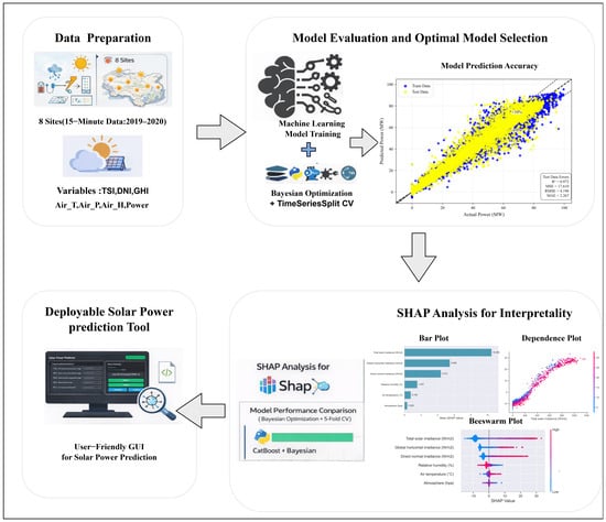
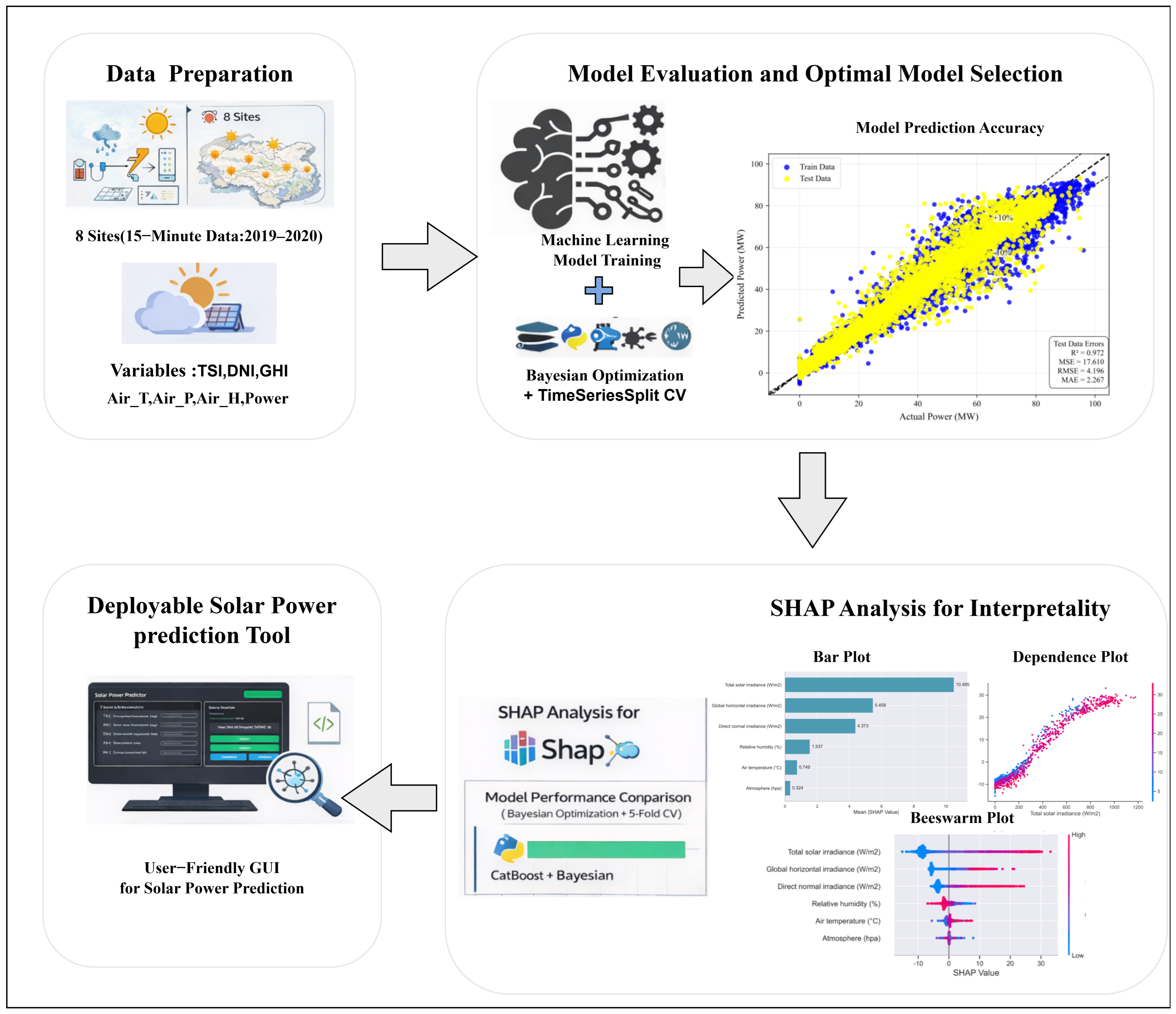
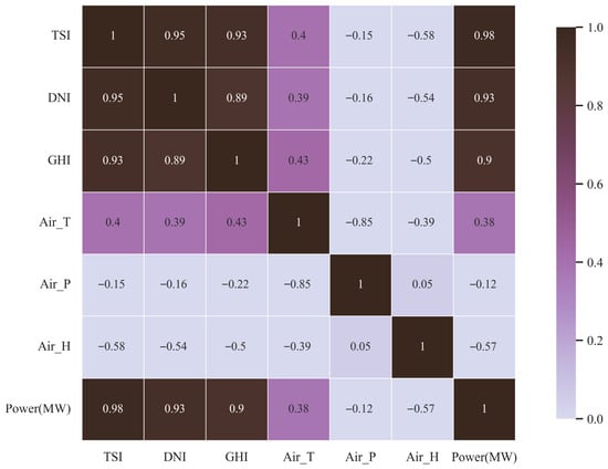
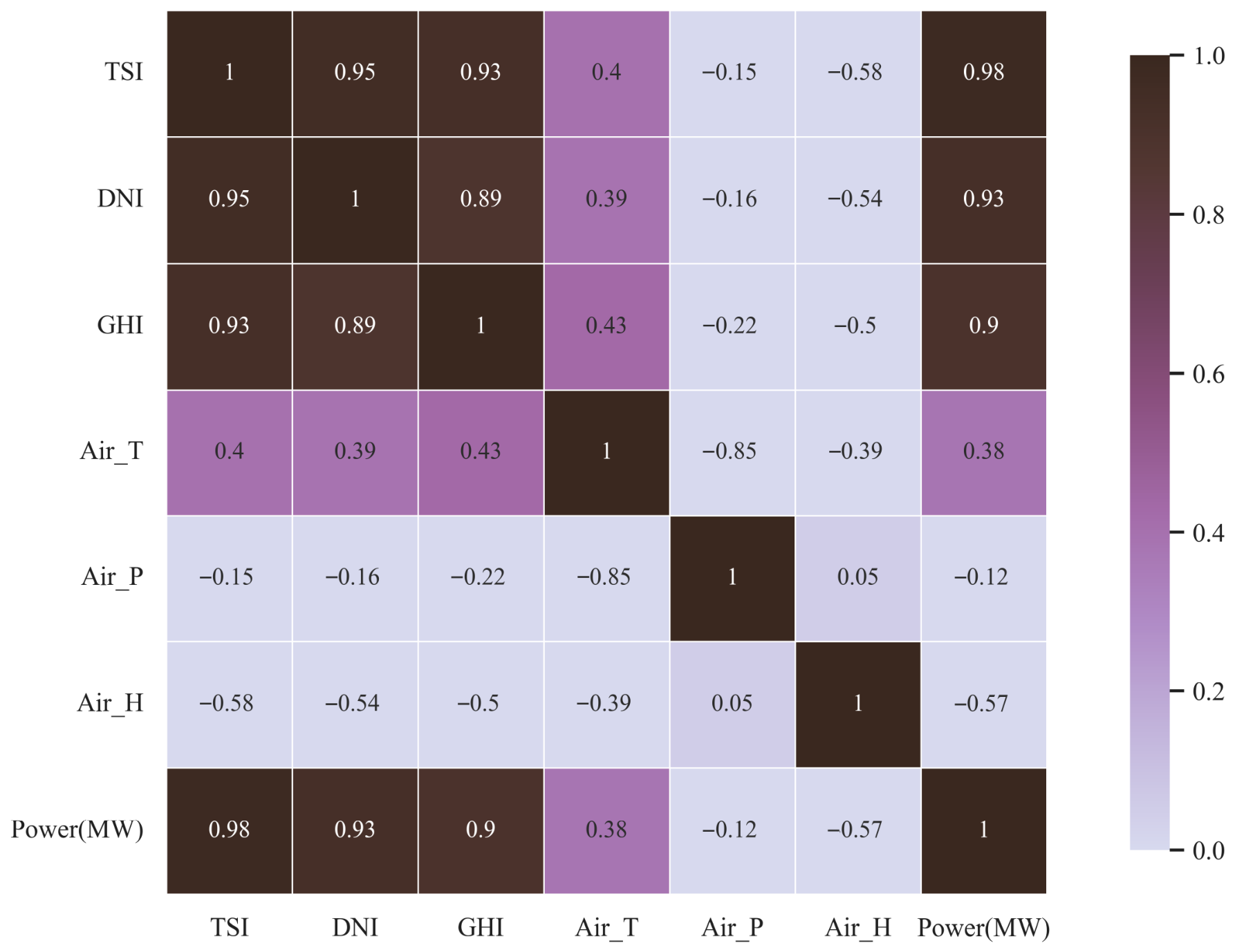
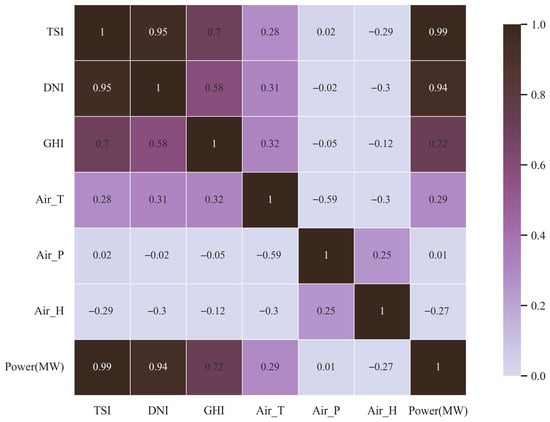
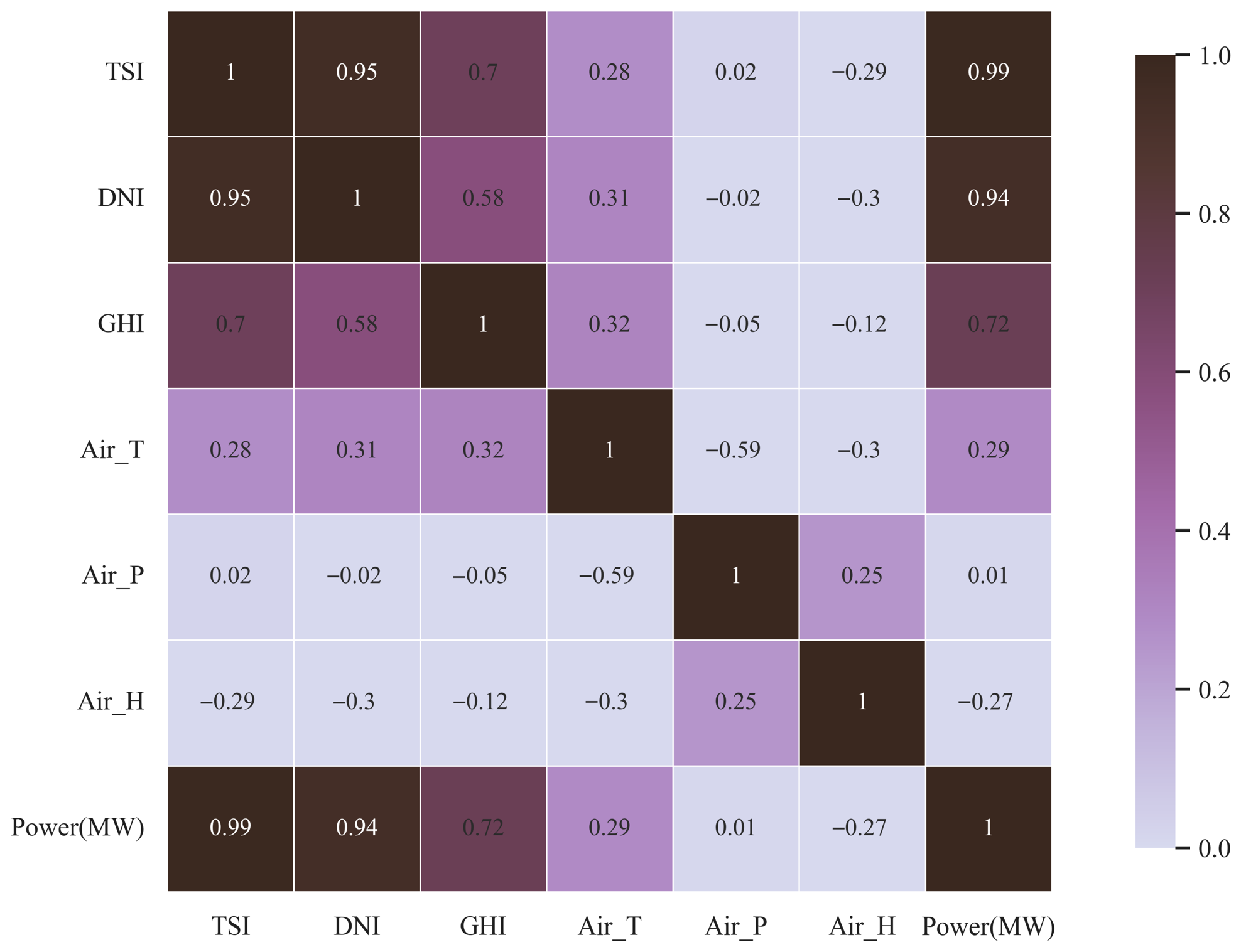
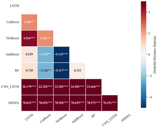
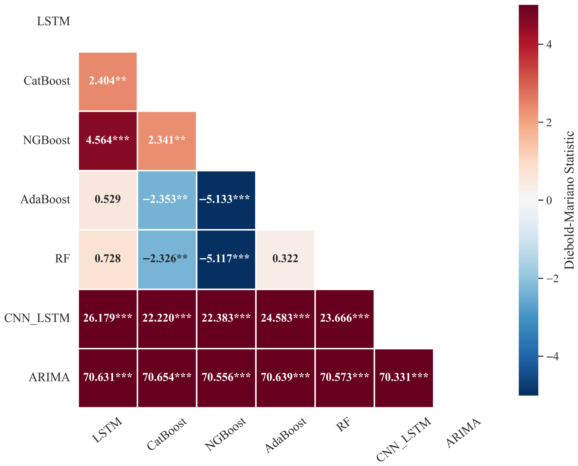
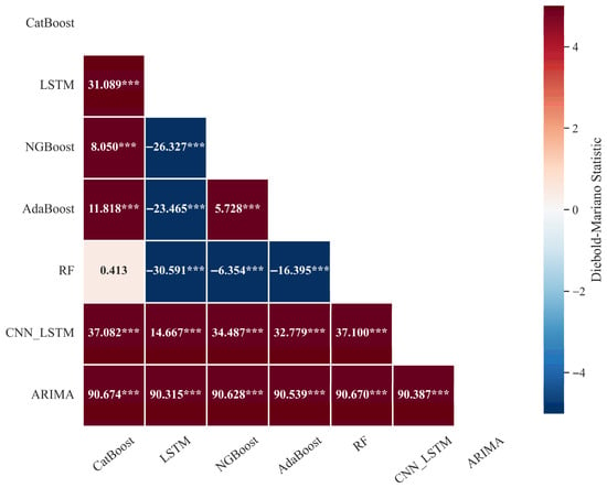
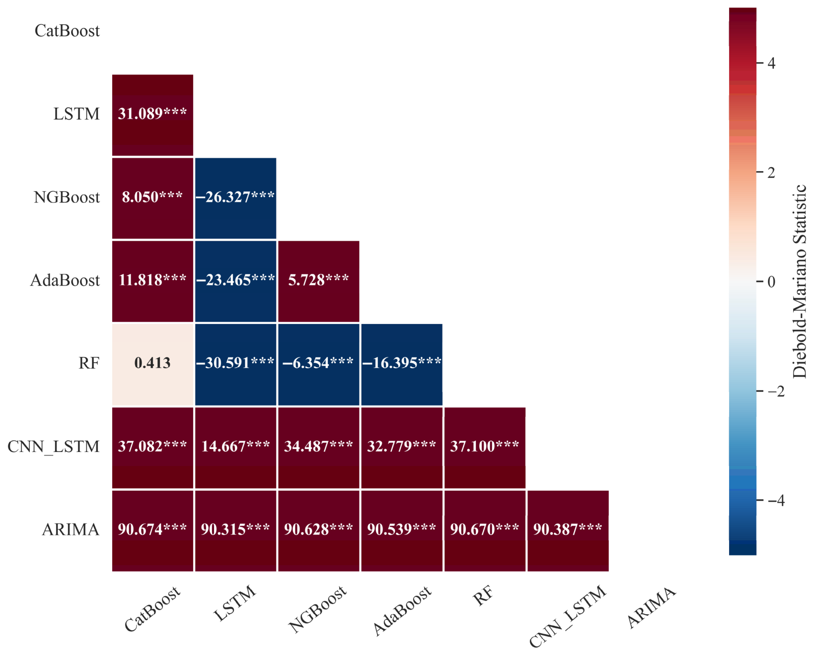
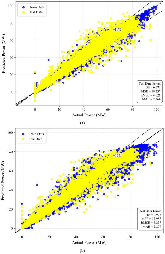
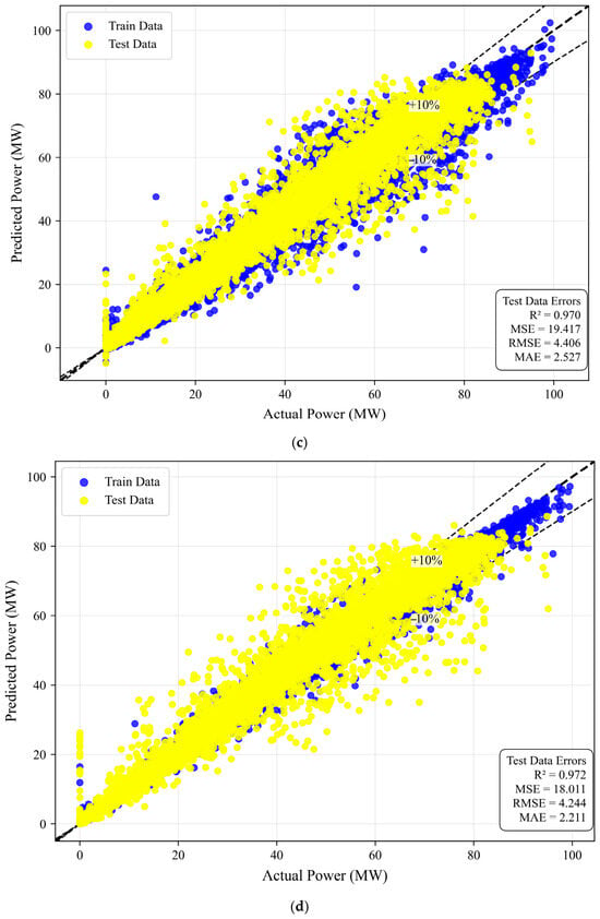
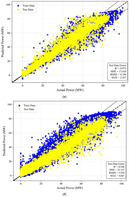
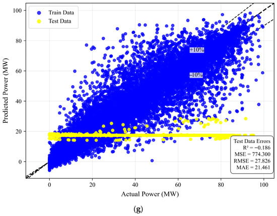
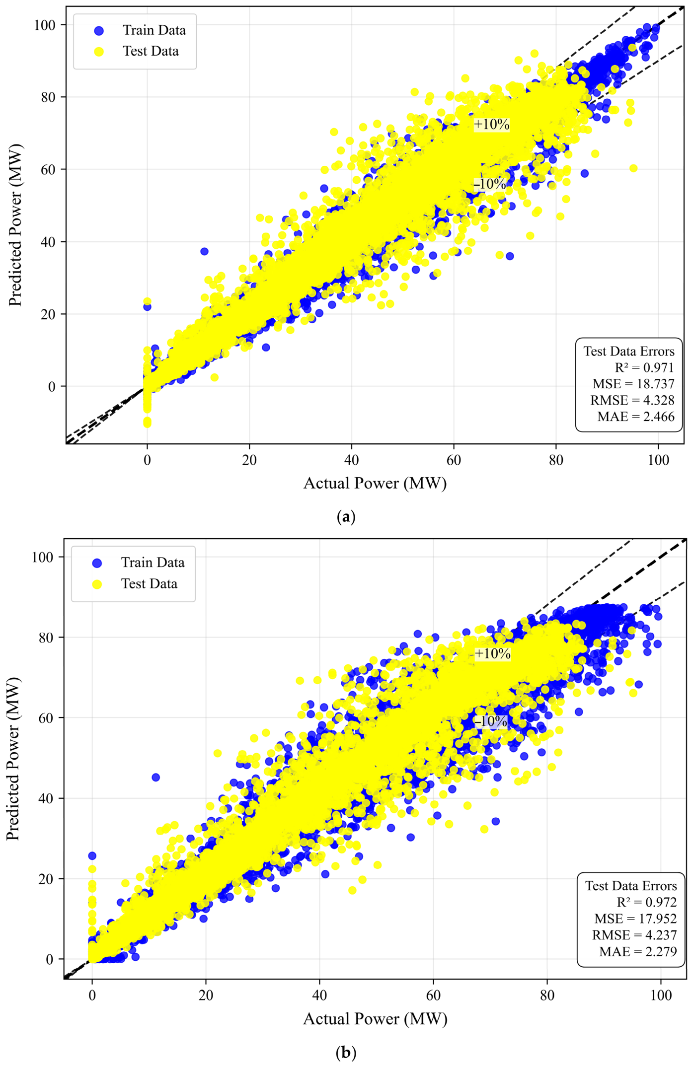
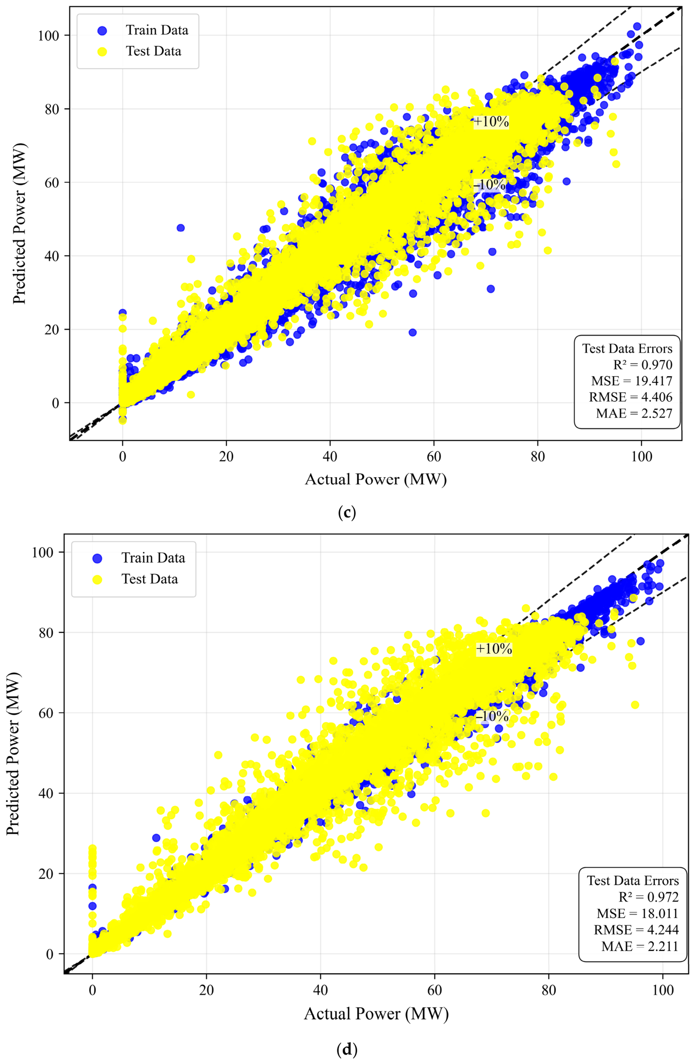
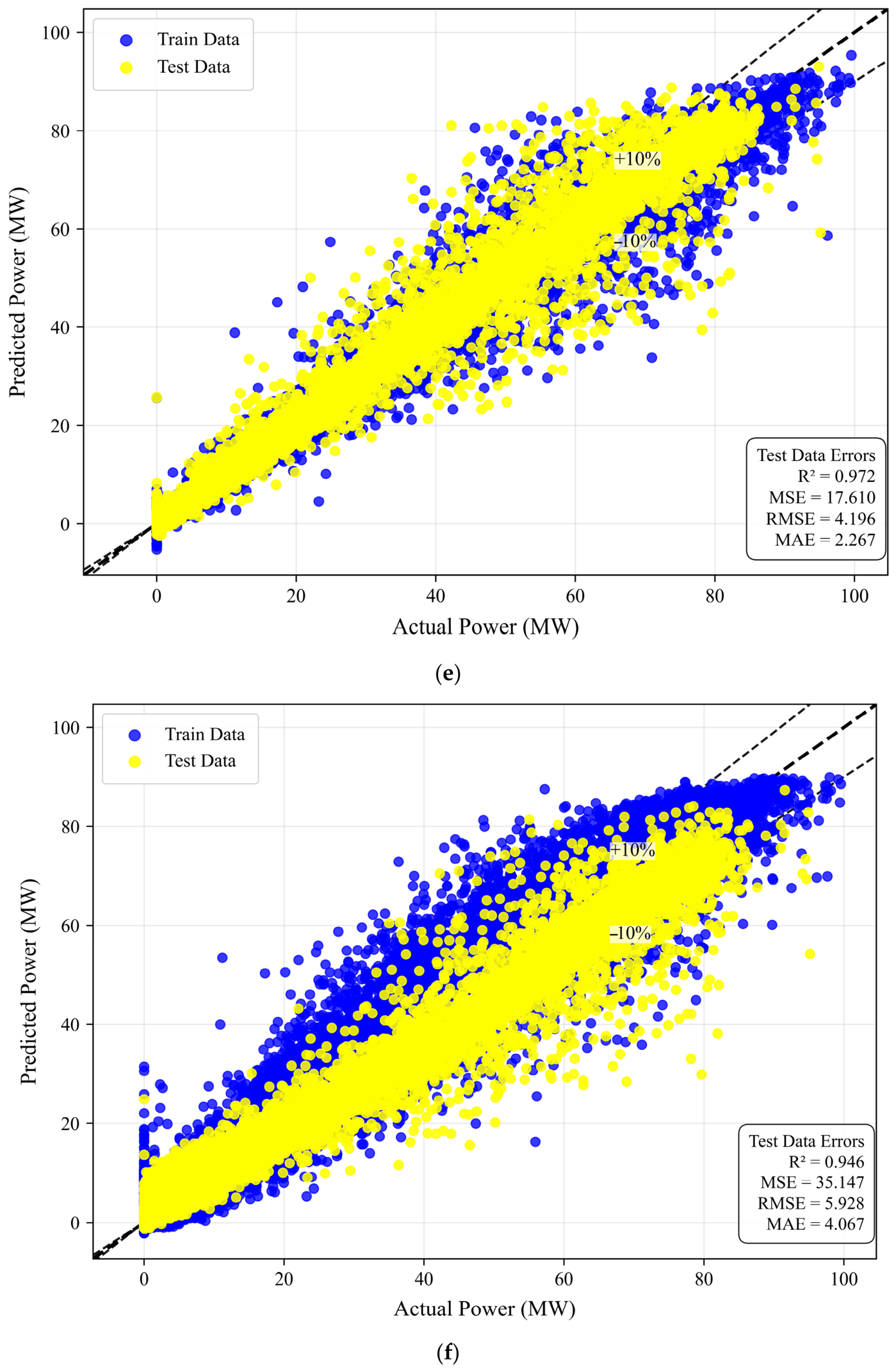
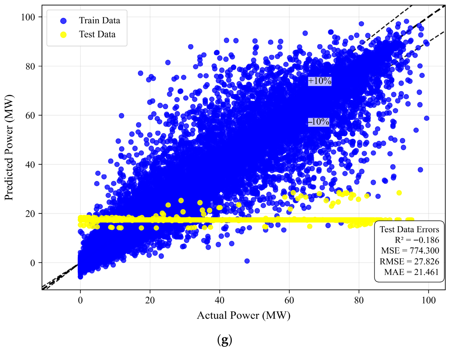
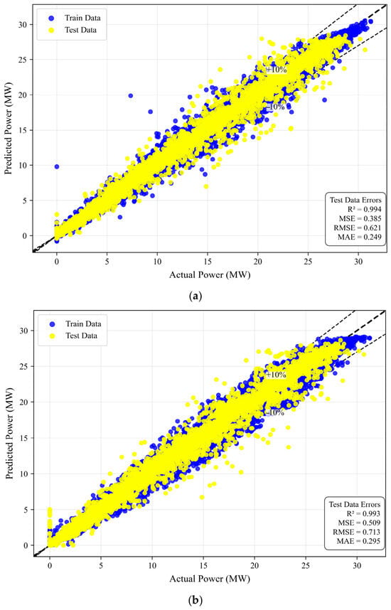
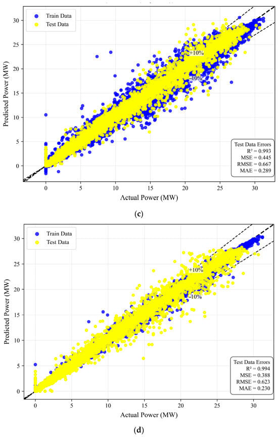
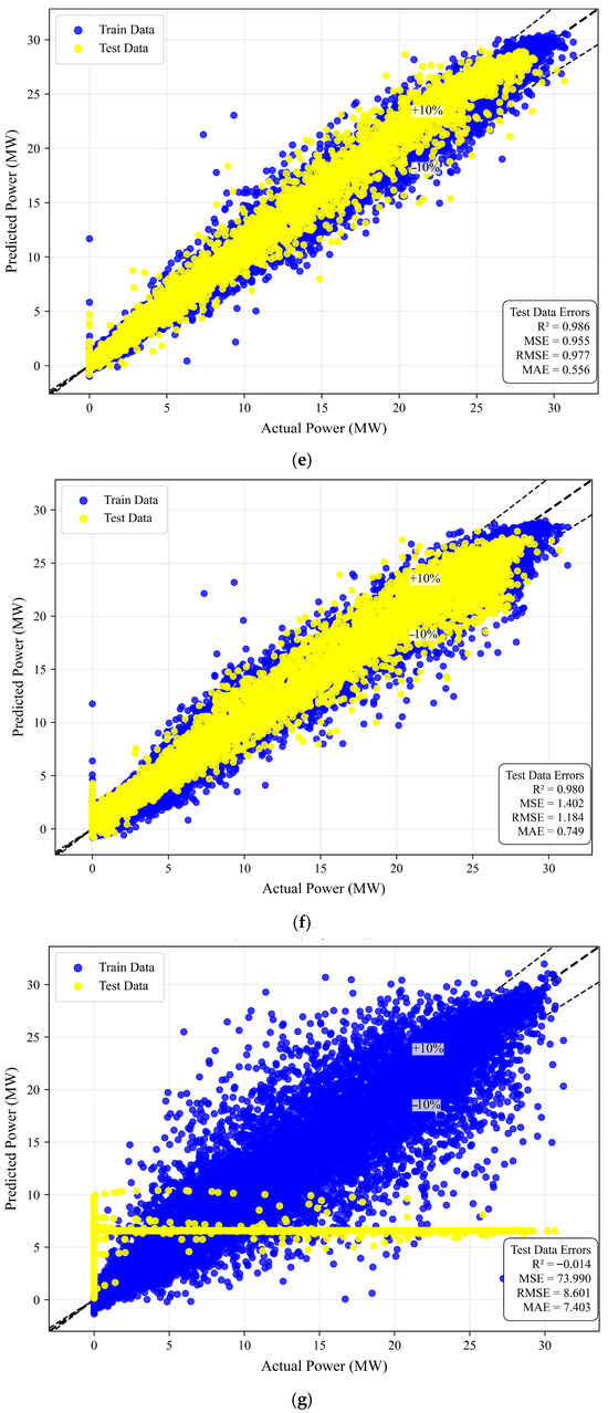
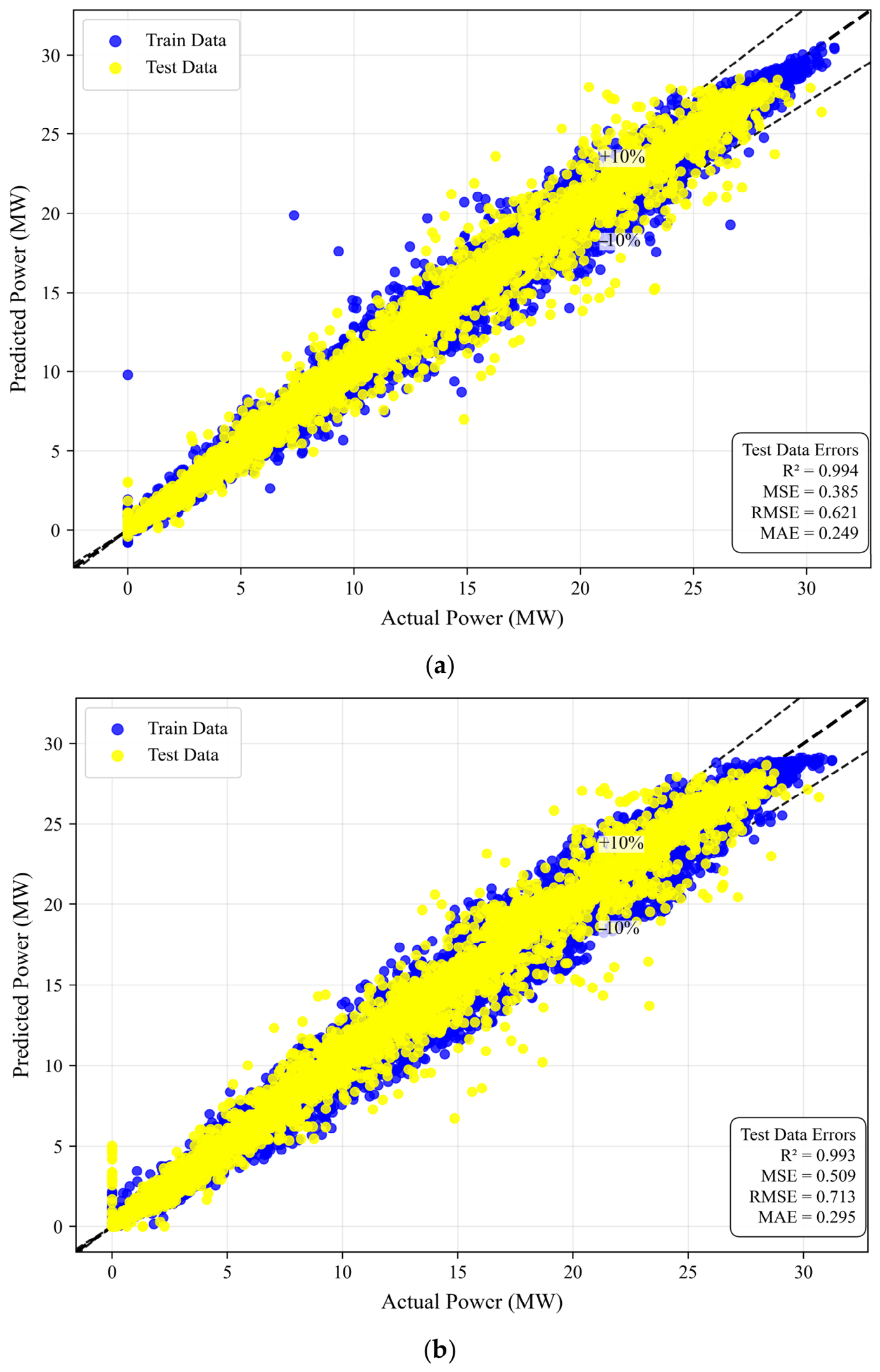
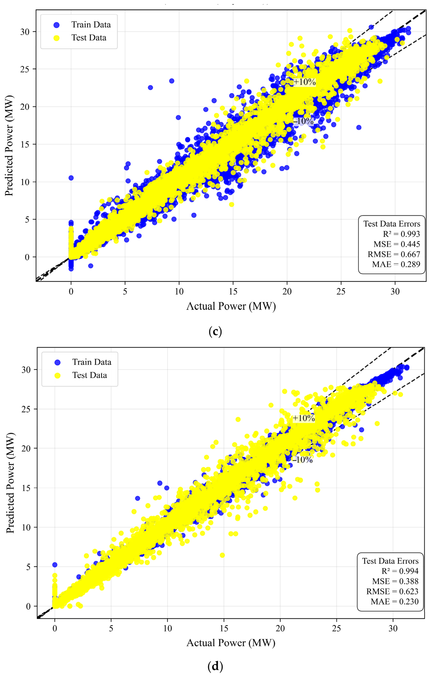
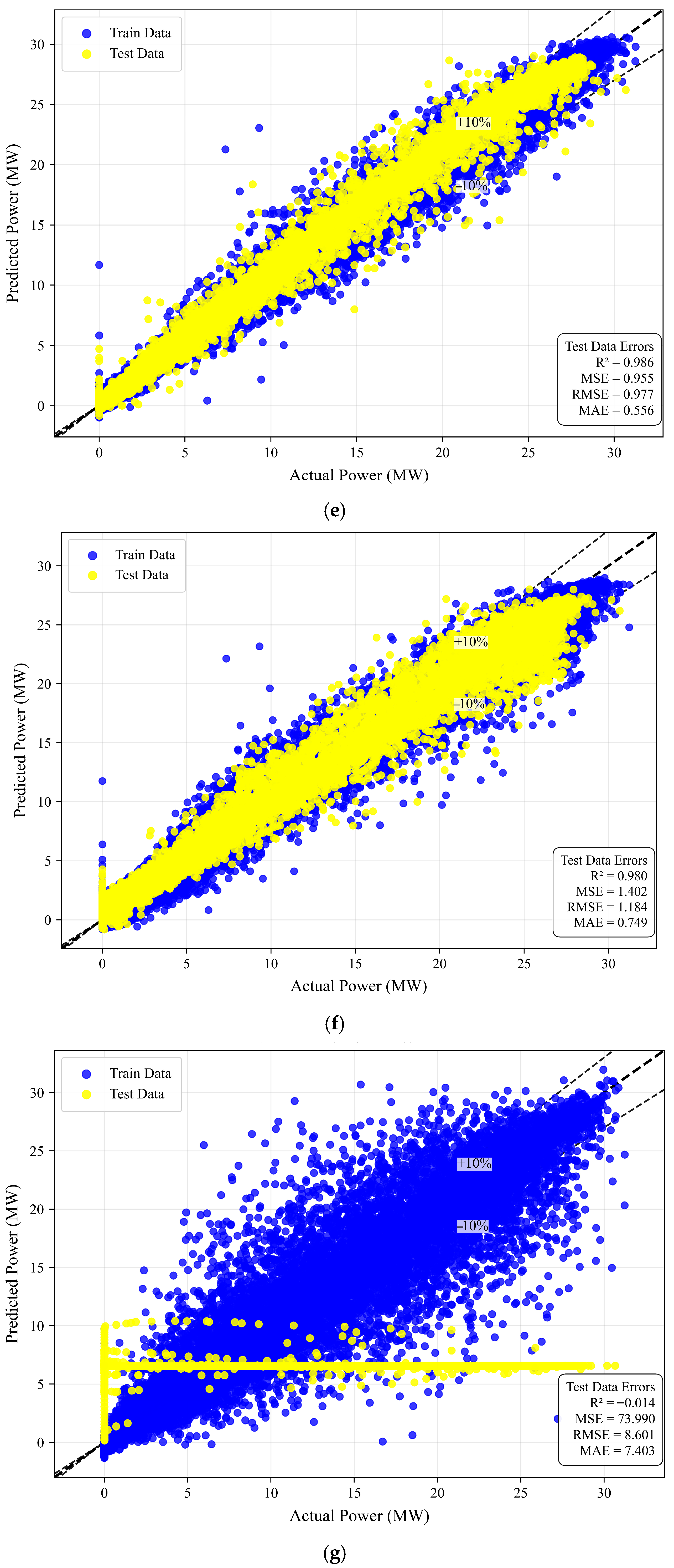
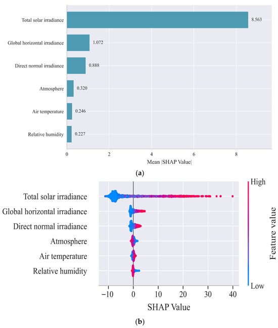
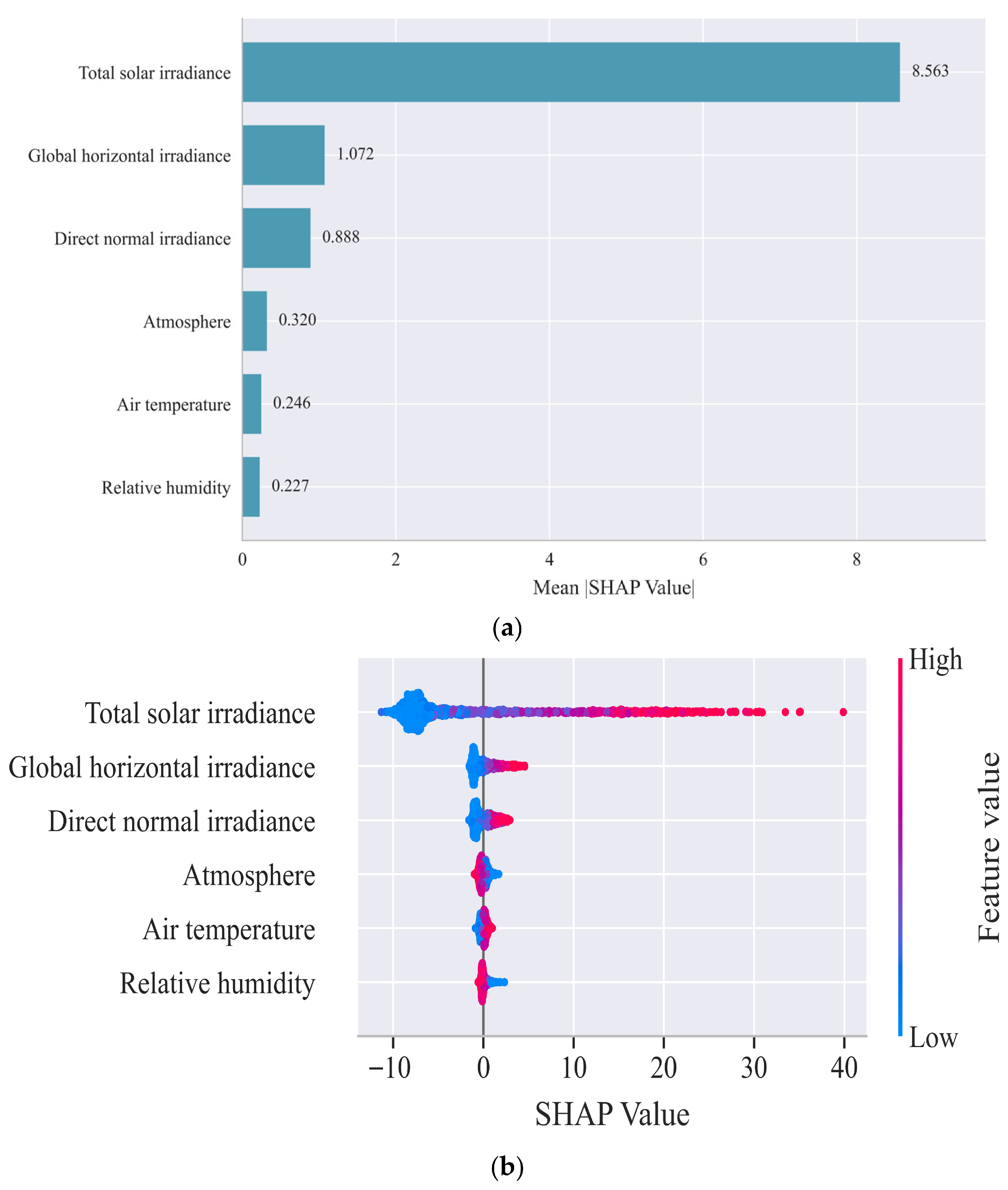
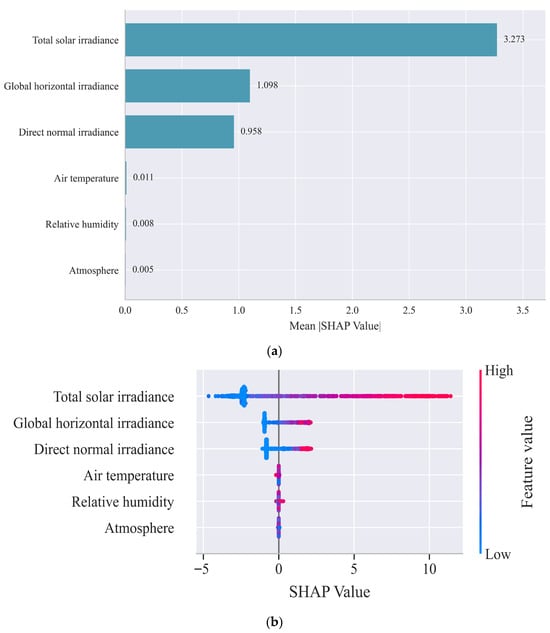
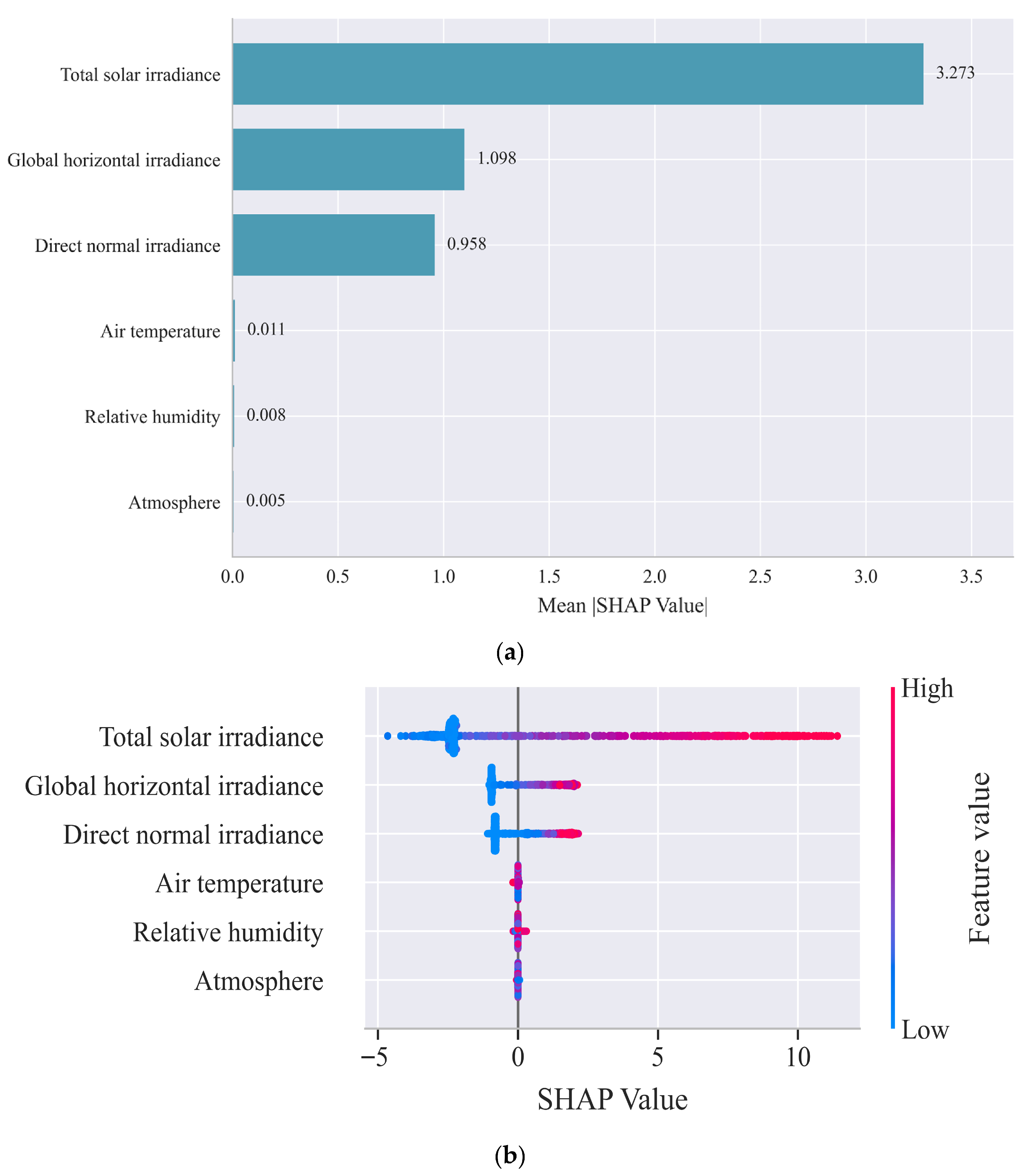
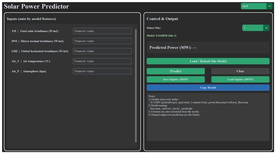
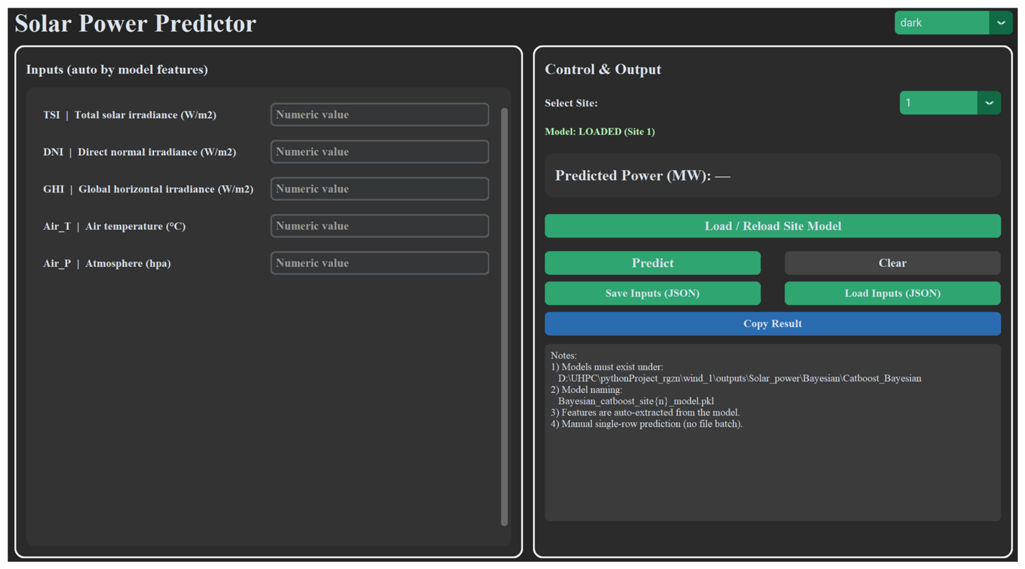

Disclaimer/Publisher’s Note: The statements, opinions and data contained in all publications are solely those of the individual author(s) and contributor(s) and not of MDPI and/or the editor(s). MDPI and/or the editor(s) disclaim responsibility for any injury to people or property resulting from any ideas, methods, instructions or products referred to in the content. |
© 2026 by the authors. Licensee MDPI, Basel, Switzerland. This article is an open access article distributed under the terms and conditions of the Creative Commons Attribution (CC BY) license.