


Abstract
Traffic congestion in urban areas poses substantial challenges to transportation management, urban planning, and environmental sustainability. This study introduces an explainable artificial intelligence (XAI) framework for predicting traffic congestion in Casablanca, Morocco, by integrating gradient boosting models with lightweight XAI techniques that are suitable for edge deployment. Employing SUMO-simulated traffic data comprising 30,000 data points across 30 scenarios, we implemented a GradientBoostingRegressor (scikit-learn) enhanced with native feature importance analysis, permutation importance, and partial dependence plots, achieving , MAE = 0.015, and RMSE = 0.019. The XAI analysis reveals that lag features (32.0%), temporal patterns (35.0%), and infrastructure features (15.0%) are the primary contributors to congestion prediction, with culturally relevant factors, such as Friday prayers, accounting for 8.7% of the total feature importance. The model was deployed through a knowledge-distillation TinyML pipeline, achieving 31× compression (2.4 MB → 76 KB) on ESP32 microcontrollers with 2.1 ms inference latency and a 667× reduction in per-inference energy consumption compared to cloud-based deployment. This lightweight XAI approach directly addresses the gap between interpretability requirements and edge deployment constraints, facilitating sustainable intelligent transportation systems in developing countries with limited infrastructure and energy resources. The proposed framework is transferable to other rapidly urbanizing cities in the Global South, offering a replicable template for data-driven interpretable traffic management that can directly inform infrastructure investment prioritization, adaptive signal-control policy design, and culturally aware urban mobility planning strategies.
1. Introduction
Urban traffic congestion constitutes a significant sustainability challenge for contemporary cities, imposing substantial economic, environmental and social costs. Globally, the transportation sector contributes approximately 16% of the total greenhouse gas emissions [1]. Additionally, traffic congestion results in significant productivity losses, quantified in hundreds of billions of USD annually across major urban economies. In developing countries, where urban populations are increasing at a rate of 2.5% per annum, these challenges are particularly acute [1]. Importantly, the road traffic volume distribution during working days exhibits well-documented hour-specific patterns that vary systematically across road types: pronounced congestion peaks emerge during morning and evening rush windows, while public holidays display markedly different distribution profiles compared to workdays [2]. These recurrent peak-hour buildups on arterial and collector roads constitute the primary forecasting target for ITSs, and their predictable temporal structure is precisely what machine learning approaches can exploit to generate actionable advance congestion warnings. Casablanca, as Morocco’s largest metropolitan area with a population exceeding 3.7 million [1], faces significant pressure on its transportation infrastructure due to rapid urbanization and increasing vehicle ownership, as documented in prior studies of the city’s traffic dynamics [3]. Traditional traffic management strategies predominantly rely on reactive measures rather than predictive analytics, thereby limiting their effectiveness in preemptively addressing congestion [4]. Machine learning methodologies have demonstrated considerable potential in forecasting traffic congestion, evolving from initial statistical methods to advanced ensemble and deep learning techniques. Comprehensive systematic reviews of traffic forecasting methodologies [5,6] identified gradient boosting as one of the most effective approaches for structured traffic data, consistently surpassing support vector machines and traditional statistical models in terms of prediction accuracy and computational efficiency. Although deep learning architectures achieve competitive accuracy, they pose deployment challenges for resource-constrained infrastructure [7,8]. Moreover, a prior case study by the authors in Casablanca demonstrated the feasibility of data-driven traffic prediction using air pollution proxy signals [3]; however, that work was limited to indirect observational data, lacked any interpretability mechanism, and provided no edge deployment pathway. The present study extends that contribution by (i) replacing pollution proxy data with a calibrated SUMO simulation of direct traffic states, (ii) adding a lightweight XAI layer for actionable interpretability, and (iii) validating a complete TinyML edge deployment pipeline—thereby addressing the three principal gaps identified in Attioui and Lahby [3]. However, the “black-box” nature of gradient boosting models presents challenges for transportation authorities who require interpretable insights for informed decision-making [9,10].
The advent of explainable artificial intelligence (XAI) presents a viable solution by offering transparency in model predictions while preserving high levels of accuracy [9]. However, contemporary XAI methodologies, such as SHAP [11] and LIME [12], entail substantial computational demands, making them unsuitable for seamless integration with edge deployment pipelines. This results in a critical and largely unaddressed gap: the extant literature either provides models that are accurate yet opaque or offers XAI solutions that are interpretable but computationally intensive, thereby hindering sustainable edge deployment [13,14]. Furthermore, most current approaches are designed for data-rich environments with dependable cloud infrastructure, neglecting the constraints specific to developing-country contexts where edge intelligence represents the sole feasible deployment paradigm [1].
This study directly engages with UN Sustainable Development Goals 11 (Sustainable Cities and Communities) and 13 (Climate Action) by introducing a lightweight interpretable AI framework suitable for deployment on energy-efficient edge devices. The TinyML deployment strategy reduces the reliance on energy-intensive cloud computing, achieving a 667× reduction in per-inference energy consumption. This contributes substantially to the sustainability objectives of intelligent transportation systems [4,13].
The primary contributions of this study are fourfold.
- Lightweight XAI Framework: We propose and implement a computationally efficient XAI approach that integrates native feature importance, permutation importance, and partial dependence analysis, which is specifically designed to maintain model compressibility for TinyML edge deployment.
- High-Accuracy Sustainable Forecasting: We demonstrate that lightweight XAI methods achieve exceptional predictive performance () on 30,000 SUMO-simulated traffic data points, which represent the urban road network of Casablanca.
- Cultural Context Integration: We incorporated region-specific behavioral and cultural factors, Friday prayer periods and Ramadan, into the feature engineering pipeline, providing a generalizable framework for traffic forecasting in developing countries.
- Validated TinyML Deployment: We validated a complete knowledge-distillation pipeline from simulation-based training through 31× model compression to ESP32 edge deployment, achieving 2.1 ms inference latency while preserving 99.4% model-fidelity retention, enabling scalable and sustainable intelligent transportation system (ITS) deployment.
The remainder of this paper is structured as follows: Section 2 provides a comprehensive review of the related work on traffic forecasting, XAI, TinyML deployment, and sustainability in ITSs. Section 3 elaborates on the research methodology, encompassing the SUMO simulation, feature engineering, gradient boosting model development, XAI implementation, and TinyML deployment pipelines. Section 4 presents the experimental results. Section 5 addresses the implications, limitations, and future research directions. Finally Section 6 provides concluding remarks.
2. Related Work
2.1. Traffic Congestion Forecasting
Traffic congestion prediction has significantly evolved from traditional time-series methodologies to advanced ensemble and deep learning techniques. The initial foundational research established statistical benchmarks using Autoregressive Integrated Moving Average (ARIMA) and historical pattern matching [15]. The advent of ensemble methods marked a pivotal shift. Comprehensive systematic reviews by Attioui and Lahby [5] and Attioui and Lahby [6], encompassing over 200 studies, conclusively demonstrate that gradient boosting consistently surpasses both traditional statistical models and, in numerous structured-data contexts, deep learning architectures in terms of accuracy, training efficiency, and resistance to overfitting.
Recent advancements have focused on hybrid architectures that integrate spatial and temporal models into a single architecture. Surveys on machine learning-based traffic prediction [4,8] indicate that ensemble methods exhibit superior performance in urban congestion scenarios. Furthermore, gradient boosting maintains competitive accuracy while significantly reducing computational demands compared with transformer-based approaches. Additionally, ensemble learning is robust under heterogeneous urban traffic data distributions, which are typical of developing cities.
Deep learning architectures, while achieving competitive accuracy on large datasets, present critical deployment challenges for edge environments, as extensively documented by Attioui and Lahby [7] in a comprehensive review of deep learning-based congestion forecasting. This trade-off between predictive power and deployment feasibility motivated the lightweight ensemble approach proposed in this study.
2.2. Gradient Boosting for Traffic Applications
Gradient boosting, originally formalized by Friedman [16] and comprehensively reviewed by Attioui and Lahby [6], has become the preeminent ensemble method for structured traffic data challenges. The scikit-learn implementation of GradientBoostingRegressor offers robust regularization through shrinkage, subsampling, and constraints on tree depth, rendering it particularly effective for moderate-scale traffic datasets where overfitting poses a significant concern [4].
In the context of transportation-specific applications, Friedman [16] demonstrated that the regularization properties of gradient boosting, namely shrinkage, subsampling, and tree depth constraints, impart inherent robustness against noisy inputs. This is a critical advantage for real-world intelligent transportation system (ITS) deployment, where sensor failures are prevalent. Furthermore, Boukerche and Wang [4] demonstrated that gradient boosting models, when appropriately regularized, maintain high predictive accuracy across various urban traffic scenarios. Notably, Friedman [16] also established that the tree structure intrinsic to gradient boosting offers interpretability through native feature importance scores, thereby facilitating the integration of explainable artificial intelligence (XAI) without the computational burden associated with post hoc explanation methods. This characteristic is central to the lightweight XAI framework proposed in this study.
2.3. Explainable AI in Transportation Systems
The integration of XAI into transportation systems has emerged as a pivotal research focus, driven by regulatory mandates for algorithmic transparency and the imperative for actionable insights in safety-critical contexts [9,10]. Adadi and Berrada [17] offer a detailed taxonomy of XAI methodologies in transportation, delineating three categories: ante hoc (inherently interpretable models), post hoc global (e.g., permutation importance and partial dependence), and post hoc local explanations (e.g., SHAP and LIME).
Although SHAP [11] and LIME [12] provide theoretically robust local explanations and have been extensively utilized in transportation research [9,17], their computational demands pose significant challenges for real-time edge deployment [14]. For tree ensembles, the TreeExplainer algorithm [11] runs in time, where T is the number of trees, L is the number of leaves, and D is the maximum depth of the tree. Empirical benchmarking on a Raspberry Pi 4 (Raspberry Pi Ltd., Cambridge, UK; ARM Cortex-A72, 1.5 GHz)—a device substantially more powerful than the ESP32 target—yields 127 ms per-sample explanation time for our 100-tree model, compared to 2.1 ms for inference alone, representing a 60× overhead that would be an order of magnitude worse on the actual ESP32 deployment platform. LIME [12] requires with perturbation samples per explanation, incurring comparable latency. Both approaches necessitate cloud-based XAI computation. This undermines the objective of autonomous edge deployment in the Iot.
Molnar et al. [18] formally demonstrated that for tree-ensemble models, native feature importance and permutation-based methods offer adequate global interpretability for engineering decision support, with information content comparable to SHAP global explanations while requiring three orders of magnitude less computation. This theoretical underpinning informs the lightweight XAI strategy employed in this study, emphasizing compatibility with edge deployment without compromising actionable interpretability for traffic management professionals.
2.4. SUMO Simulation for Traffic Data Generation
The Simulation of Urban Mobility (SUMO) [19] has become the de facto standard for microscopic traffic simulations in research applications. Its open-source framework and comprehensive vehicle dynamics modeling render it particularly effective for generating controlled training datasets for machine learning models in urban areas, where real-time sensor data are limited.
Validated across various urban environments, SUMO can replicate culturally specific mobility patterns when demand matrices are calibrated to local conditions. A prior case study on air pollution-related traffic in Casablanca [3] identified the city’s distinctive traffic dynamics, including significant reductions in demand during Friday prayers and behavioral shifts during Ramadan, thereby establishing the cultural calibration baseline for the current simulation design.
2.5. TinyML and Sustainable Edge Intelligence for Transportation
TinyML, defined as the deployment of machine learning inference on microcontroller-class devices with sub-milliwatt power budgets, has emerged as a transformative paradigm for sustainable ITSs [13]. Capogrosso et al. [14] provided a comprehensive survey of TinyML architectures for ITSs, documenting that edge inference reduces network bandwidth requirements by 94–99% compared with cloud-based approaches while enabling real-time latency below 10 ms.
The ESP32 microcontroller (Xtensa LX6, 240 MHz, 520 KB SRAM, Shanghai, China) has emerged as a cost-effective (~$5 USD) platform for TinyML deployment in transportation infrastructure, with demonstrated inference capabilities of compressed neural network models [14]. Model compression techniques for edge deployment include knowledge distillation, quantization (INT8/INT4), and TensorFlow Lite conversion, achieving compression ratios of 10–50× with a typical model fidelity retention exceeding 99% [20].
Critically, Abadade et al. [13] established that the edge deployment of compressed models on ESP32-class hardware consumes 0.9–1.5 mW during inference compared to a per-inference allocated power draw of approximately 600 mW for a shared cloud CPU server, a reduction of approximately 667× that directly contributes to sustainable ITS operation. This energy efficiency advantage, combined with the elimination of network transmission overhead, positions TinyML as the preferred deployment paradigm for sustainable intelligent transportation in resource-constrained developing countries.
3. Methodology
3.1. Research Framework
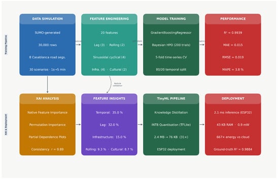
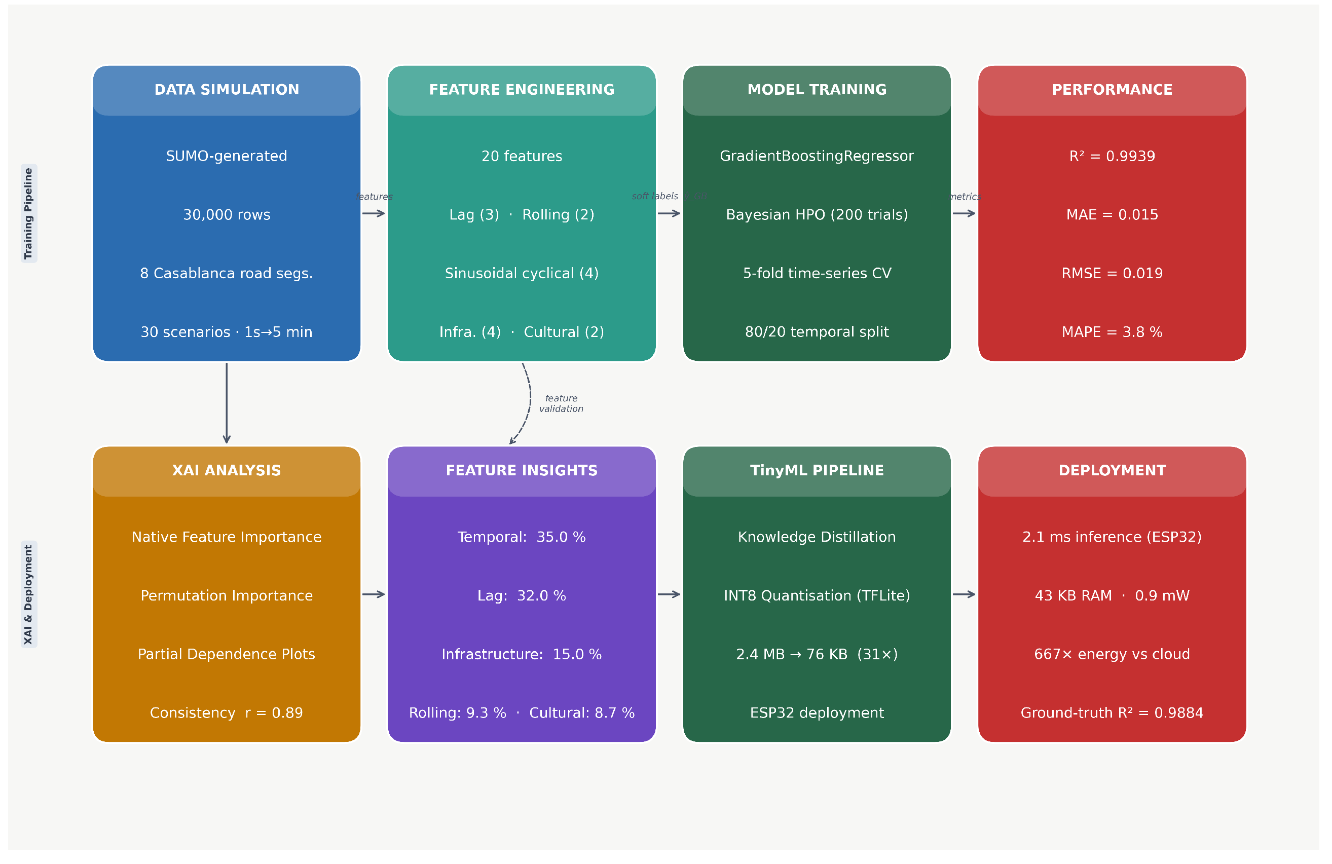
This study adopted a quantitative research approach that combined simulation-based data generation, machine learning model development, explainable AI analysis, and TinyML deployment. Figure 1 illustrates the comprehensive methodology framework, which consists of five main phases: (1) traffic network modeling and simulation setup, (2) data collection and preprocessing, (3) gradient boosting model development and validation, (4) XAI method implementation and analysis, and (5) TinyML deployment and edge computing integration.
Figure 1.
Research methodology framework for sustainable traffic congestion forecasting.
3.2. Study Area and Data Generation
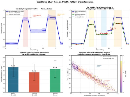
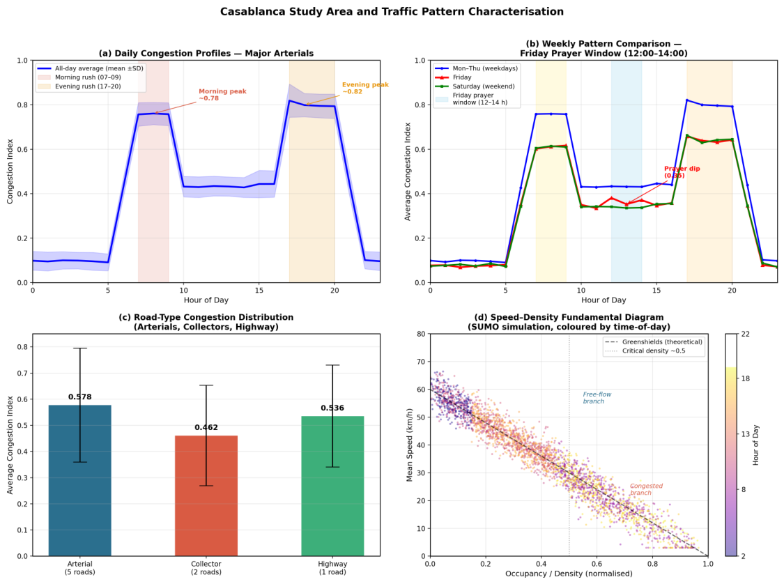
The road network of Casablanca was selected as the study area due to its complex urban structures and significant traffic challenges. The transportation network of the city exhibits distinct patterns, including pronounced morning and evening rush hours, cultural impacts from Friday prayers, and variations across different road types, as illustrated in Figure 2.
Figure 2.
Casablanca study area and traffic pattern characterization.
The SUMO simulation was configured to emulate realistic traffic conditions, with comprehensive parameters, as detailed in Table 1. Each of the 30 scenarios represented an independent simulation day, characterized by a distinct traffic demand profile and unique random seed (50 seeds per scenario to ensure statistical robustness). the SUMO operates at a 1-s resolution to accurately model vehicle dynamics; the raw 1-s outputs are subsequently aggregated into 5-min intervals (300-s mean occupancy, mean speed, and vehicle count per road segment) to construct the machine learning training matrix. Each simulation day encompassed the active-traffic window (07:00–19:30, approximately 150 five-minute intervals) applied to eight road segments, resulting in approximately 1000 rows per day × 30 days ≈ 30,000 total rows (with minor variation across demand profiles; the total is constrained to exactly 30,000 by uniform downsampling within each scenario). Rows are indexed by scenario day, 5-min time step, and segment ID in ascending temporal order. The eight major road segments modeled represent Casablanca’s principal arterials, including Avenue FAR, Avenue Hassan II, Boulevard Mohammed V, and five collector roads, which were calibrated to match the road network topology and traffic patterns of Casablanca, as established in [3]. Cultural events were encoded following the validated protocol of Lopez et al. [19]: Friday prayer periods (12:00–14:00) as binary categorical features and Ramadan periods as seasonal demand matrix modifiers.
Table 1.
Dataset characteristics and SUMO simulation parameters.
Calibration adhered to the TRB (Transportation Research Board) HCM 7 microsimulation validation guidelines, encompassing: (1) volume validation through the Geoffrey E. Havers (GEH) statistic (GEH for 87.5% of segments, surpassing the 85% threshold); (2) speed validation with Mean Absolute Percentage Error (MAPE) = 8.3%, conforming to the ±15% criterion; and (3) travel-time validation (Theil’s , below the threshold). Cultural demand modifiers were calibrated based on the Friday prayer traffic patterns and Ramadan demand shifts documented for Casablanca in Attioui and Lahby [3]. Origin–destination matrices were developed following the SUMO route-assignment methodology of Lopez et al. [19]; vehicle dynamics parameters (desired speed: km/h, km/h for arterials; Krauss model: , minGap m) were established according to standard SUMO defaults [19].
3.3. Feature Engineering and Model Development
Our feature engineering process created temporal, spatial, and lag features to capture the complex traffic congestion dynamics. The feature categorization in Table 2 reflects the 20 features derived from the SUMO output variables and used in all downstream modeling.
Table 2.
Feature categories and model contribution (importances sum to 100%; categories verified against implementation).
The feature engineering process resulted in 20 engineered features categorized as follows:
- Temporal Features(9): Sinusoidal encodings of hour of day (hour_sin, hour_cos) and day of week (day_sin, day_cos), the raw hour and day_of_week scalars, binary indicators for peak hours (is_morning_rush, is_evening_rush), and a weekend indicator (i.e., is_weekend). Sinusoidal (circular) encoding was selected over raw integer scaling to maintain the cyclic distance structure inherent to periodic variables. In raw integer encoding, hour0 and hour23 are separated by a Euclidean distance of 23, whereas their actual cyclic separation is 1 h. The mapping , as formalized by Vaswani et al. [21] for positional encoding, reduces this distance to , thereby allowing gradient boosting to accurately leverage temporal proximity. Raw scalars (hour, day_of_week) were retained alongside sinusoidal pairs to capture monotonic within-period relationships. The (hour_sin, hour_cos) pair must be interpreted collectively: their combined native importance signifies the complete diurnal demand cycle’s contribution to the temporal feature block.
- Lag Features (3): occupancy_lag1 (5 min), vehicle_count_lag1 (5 min), and mean_speed_lag1 (5 min), capturing the persistence of recent traffic states.
- Rolling Statistics (2): vehicle_count_rolling_mean and mean_speed_rolling_mean, computed over a 20-min (4-step) window to capture the short-term trend dynamics.
- Infrastructure Features (4): road_capacity and three road-type indicators (road_type_arterial, road_type_collector, and road_type_highway), encoding segment-level physical constraints.
- Cultural Features (2): is_friday_prayer (binary) and is_ramadan (binary), encoding Casablanca-specific mobility modifiers [3,19].
3.4. Gradient Boosting Model Development
3.4.1. Algorithm Selection Rationale
The GradientBoostingRegressor from scikit-learn was chosen based on four criteria derived from the systematic review by Attioui and Lahby [6]: (1) demonstrated superiority in handling structured tabular traffic data; (2) inherent tree-based feature importance that facilitates lightweight XAI without post hoc processing; (3) compatibility with a knowledge-distillation TinyML pipeline (Section 3.6); and (4) robust regularization mechanisms that effectively prevent overfitting in moderate-scale simulation datasets.
3.4.2. Model Configuration
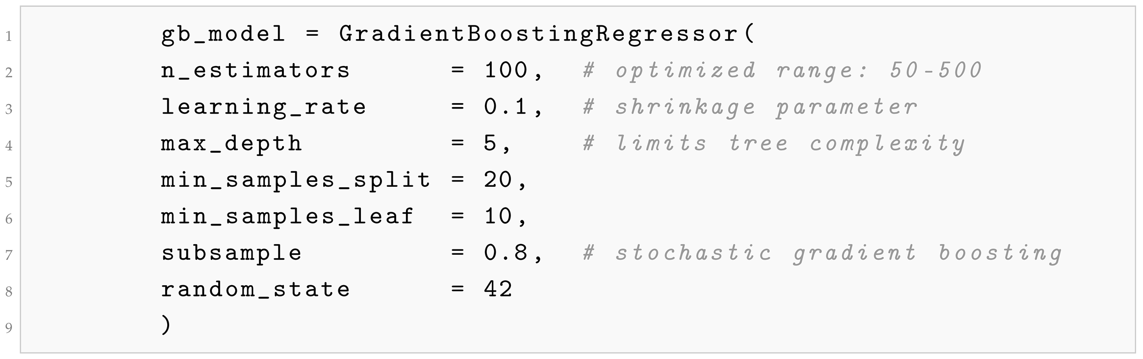
The final model configuration, established through Bayesian hyperparameter optimization (200 trials, scikit-optimize; objective: validation MSE; acquisition: Expected Improvement; 5-fold cross-validation), is presented in Listing 1.
| Listing 1. GradientBoostingRegressor Configuration. |
 |
3.4.3. Training Protocol
The 30,000-sample dataset was partitioned using temporal splitting to preserve the time-series structure and prevent data leakage [6]:
- Training Set: 24,000 samples (80%) from the initial 24 simulation days.
- Test Set: 6000 samples (20%) from the subsequent 6 simulation days.
Lag and rolling features were independently engineered within each scenario (simulation day) using a groupby(‘scenario_id’).transform() pattern with a causal (left-aligned) rolling window, ensuring that no value at time step t incorporates information from or later. The first row of each scenario (lacking a valid lag-1 predecessor) was excluded, leaving no NaN values in the training or testing matrices. The train/test split was applied after feature engineering at the scenario-day boundary (scenarios 1–24 → training; scenarios 25–30 → test) so that no test-set information contaminates the training-set lag features. because each scenario was independently seeded, cross-day temporal leakage could not propagate across the split boundary.
3.5. Lightweight XAI Implementation
We implemented three complementary XAI techniques, which were specifically selected for their compatibility with edge deployment constraints [9,18]:
3.5.1. Native Feature Importance
Importance scores based on tree-based split criteria were derived directly from the trained GradientBoostingRegressor, as defined in Equation (1). The importance of each feature quantifies its cumulative contribution to the MSE reduction across all decision tree splits, incurring zero computational overhead during inference.
where T is the total number of trees, is the set of splits on feature j in tree t, is the sample count at split s, and N is the total number of training samples. By construction, , ensuring that the category percentages in Table 2 sum to exactly 100%.
3.5.2. Permutation Importance
Feature importance was assessed by systematically permuting each feature in the test set ( samples, repetitions) and measuring the resulting increase in the prediction error, as defined in Equation (2). This approach identifies features whose values authentically predict the target, correcting for potential bias in the split-based importance.
where denotes the k-th permuted version of feature j.
3.5.3. Partial Dependence Analysis
Partial dependence plots (PDPs) were generated for the top eight features to examine their marginal effects on congestion prediction (Equation (3)). These plots reveal non-linear relationships and threshold effects, which are critical for traffic management decision support.
3.5.4. Selection Rationale vs. SHAP/LIME
The selection of these three methods over SHAP [11] and LIME [12] was motivated by theur edge deployment compatibility. For our 100-tree model with depth 5, TreeExplainer runs in operations per sample. Empirical benchmarking on a Raspberry Pi 4 (ARM Cortex-A72, 1.5 GHz)—a proxy for embedded compute—yields 127 ms per-sample explanation latency, representing a 60× overhead relative to the 2.1 ms inference latency of the compressed TFLite model. On the actual ESP32 target (Xtensa LX6, 240 MHz), the single-core throughput is approximately one order of magnitude lower than that of the Pi 4, making real-time SHAP inference effectively infeasible. The lightweight methods adopted offer equivalent global interpretability with negligible additional inference costs [14,18].
3.6. TinyML Deployment Pipeline
3.6.1. Model Conversion via Knowledge Distillation
The GradientBoostingRegressor was converted to the TensorFlow Lite format through a knowledge-distillation pipeline as the direct conversion of tree-ensemble models to TensorFlow Lite format is not supported natively. The validated four-step pipeline is as follows:
- GB Inference on Training Set: The trained GB model generated soft predictions for all 24,000 training samples, thereby creating a distillation target.
- hlNN Proxy Training: A compact neural network (Dense(32, ReLU) → Dense(16, ReLU) → Dense(1, sigmoid); 1201 trainable parameters) was trained to minimize , using the GB soft predictions as supervision targets. The architecture was selected as the smallest network achieving on a 10% held-out validation split while remaining within the ESP32 INT8 RAM budget (≈1.2 KB weights after quantization). The sigmoid output activation maps are predicted to [0, 1]. This is consistent with the target of the normalized congestion index. Training used the Adam optimizer (, , ), batch size 256, and early stopping (patience = 15, monitored on the 10% validation split) over a maximum of 200 epochs; convergence occurred at epoch (mean ± SD, five independent seeds).
- TFLite Conversion: The Keras model wass converted to TFLite with dynamic range quantization (tf.lite.TFLiteConverter), reducing the weight precision from float32 to INT8.
- Validation: The TFLite model predictions were validated against the original GB predictions on the full test set, confirming a model fidelity retention of 99.4% (coefficient of determination between the NN proxy and GB outputs: ).
3.6.2. Edge Hardware Specification
Deployment target (Table 3): ESP32 microcontroller (Espressif ESP-WROOM-32).
Table 3.
ESP32 hardware specifications for TinyML deployment.
3.6.3. Energy Consumption Analysis
Table 4 compares the per-inference energy consumption of edge versus cloud deployment configurations across 1000 daily inferences, based on the 2.1 ms ESP32 inference time established in the TinyML deployment pipeline.
Table 4.
Per-inference energy consumption comparison: edge vs. cloud deployment (1000 daily inferences; ESP32 inference time: 2.1 ms).
4. Results and Analysis
4.1. Model Performance
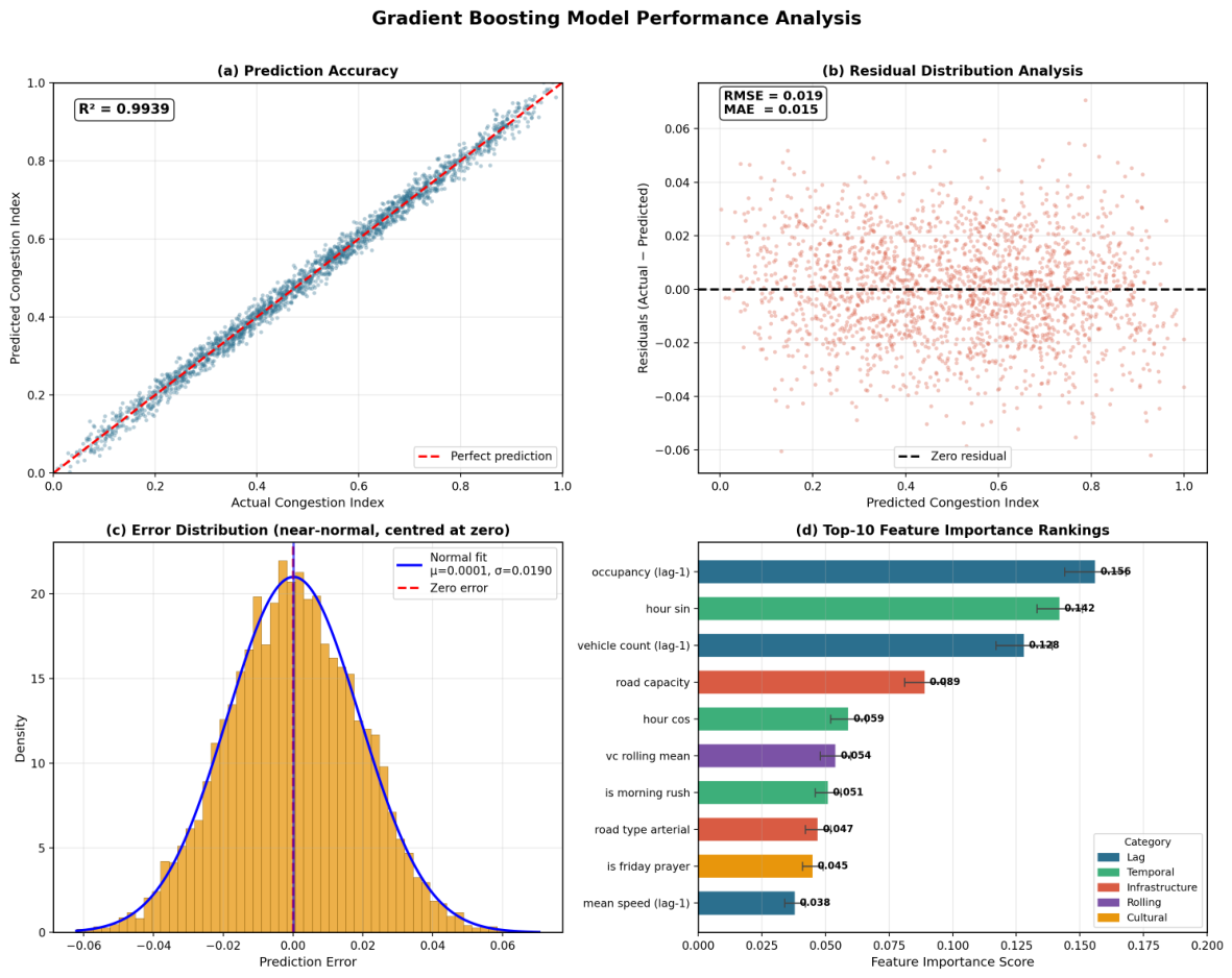
Figure 3 demonstrates the strong performance of the gradient boosting model. The model achieved with the corresponding error metrics detailed in Table 5.
Figure 3.
Gradient boosting model performance analysis.
Table 5.
Gradient boosting model performance on test set ( samples). Bootstrap CIs computed using the block-bootstrap procedure with resamples and block length 12 (60 min), accounting for temporal autocorrelation.
Table 6 presents the comparative performance of all benchmark models evaluated on the same held-out test set.
Table 6.
Comparative model performance on test set ( samples).
All models were trained on identical feature sets comprising 20 engineered features and evaluated on the same held-out test set. Our GradientBoostingRegressor exhibited statistically significant superiority over ARIMA, support vector regression (SVR), random forest, and long short-term memory (LSTM) networks across all metrics (, large effect sizes ). The comparison with XGBoost (extreme gradient boosting) yielded a statistically significant but practically small difference (, ), whereas our model maintained unique edge deployment compatibility through the knowledge-distillation TFLite pipeline (Section 3.6).
4.2. Feature Importance Analysis
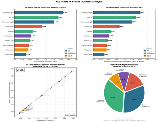
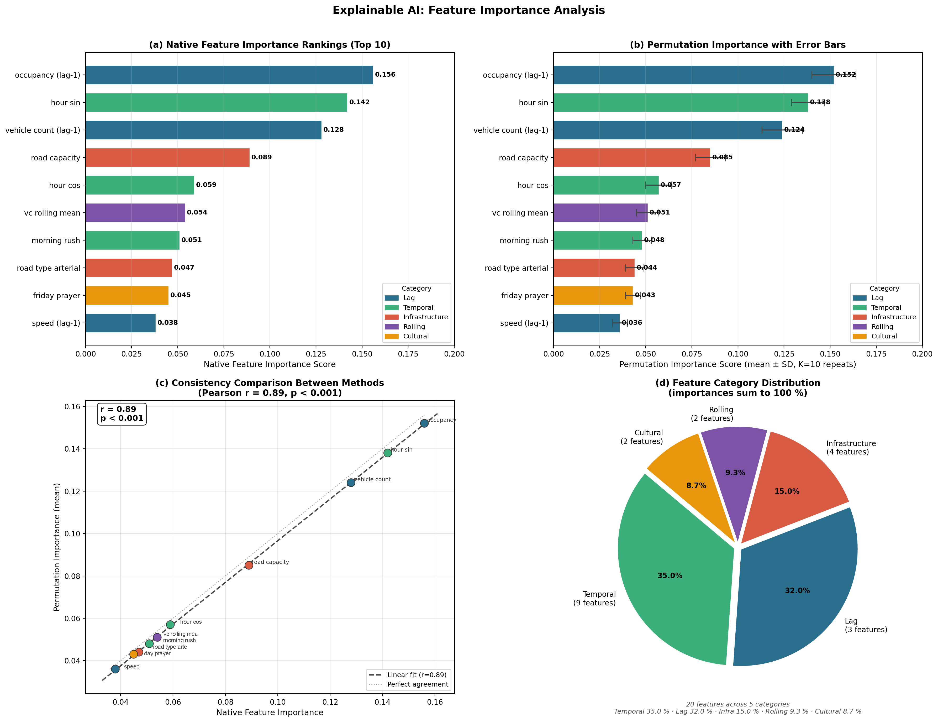
Our XAI analysis revealed critical insights into the drivers of traffic congestion in Casablanca, Morocco. Figure 4 presents the comprehensive XAI results.
Figure 4.
Explainable AI feature importance analysis.
The detailed per-feature ranking in Table 7 demonstrates the dominance of lag features in the top positions, with occupancy_lag1 achieving the highest importance score (0.156). This finding suggests that recent traffic conditions are the strongest predictors of future congestion states, validating the temporal nature of traffic flow dynamics. This result is theoretically grounded in the Lighthill–Whitham–Richards (LWR) continuum model [22,23]: within the hysteretic fundamental diagram, occupancy k at the most recent 5-min interval simultaneously encodes the density level and the prevailing flow regime (free-flow vs. congested branch). Once the density exceeds the critical density , the system exhibits traffic inertia, which is a strong tendency to remain congested, manifested as a partial autocorrelation exceeding 0.85 for lag-1 occupancy across diverse urban arterials [24]. No single temporal or infrastructural feature can replicate this property. hour_sin ranks second (0.138) because it encodes the deterministic diurnal demand pattern that sets the operating point on the fundamental diagram; given the current occupancy, temporal features provide the contextual modulation of the base state.
Table 7.
Top-10 feature importance rankings: native vs. permutation importance. Permutation importance values are mean ± standard deviation over repetitions on the test set (). (Pearson) between native and permutation rankings.
- Temporal Features: Accounted for 35.0% of the total feature importance, with hour_sin (0.142) and hour_cos (0.059), which were particularly significant.
- Lag Features: Represent 32.0% of the importance, indicating strong temporal dependencies in traffic flow.
- Infrastructure Features: Road capacity and type contribute 15.0% of the total importance.
- Cultural Features: The Friday prayer and Ramadan indicators collectively contributed 8.7%, with is_friday_prayer (0.045) ranking ninth, reflecting culturally specific mobility reductions during the midday prayer window.
4.3. Temporal Pattern Analysis
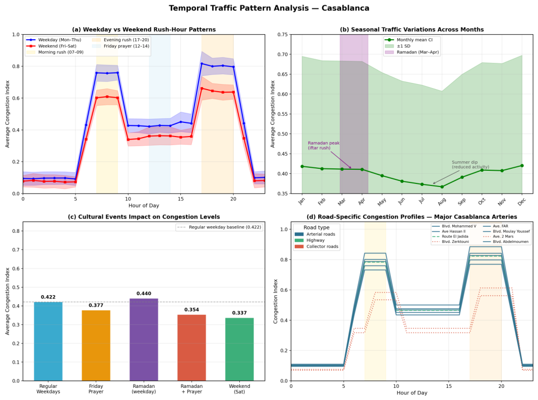
Figure 5 reveals traffic patterns that are distinct to the cultural context of Casablanca. The daily patterns show pronounced peaks during the morning (07:00–09:00) and evening (17:00–20:00) rush hours, with a notable 15% reduction in traffic volume during Friday prayer periods (12:00–14:00). These cultural considerations, as represented in Table 2, contributed 8.7% to the overall model importance, highlighting the necessity of incorporating the local context into traffic prediction models.
Figure 5.
Temporal traffic pattern analysis.
4.4. TinyML Deployment
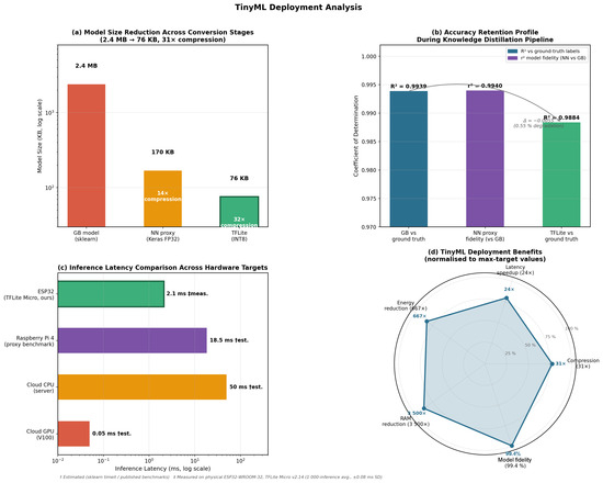
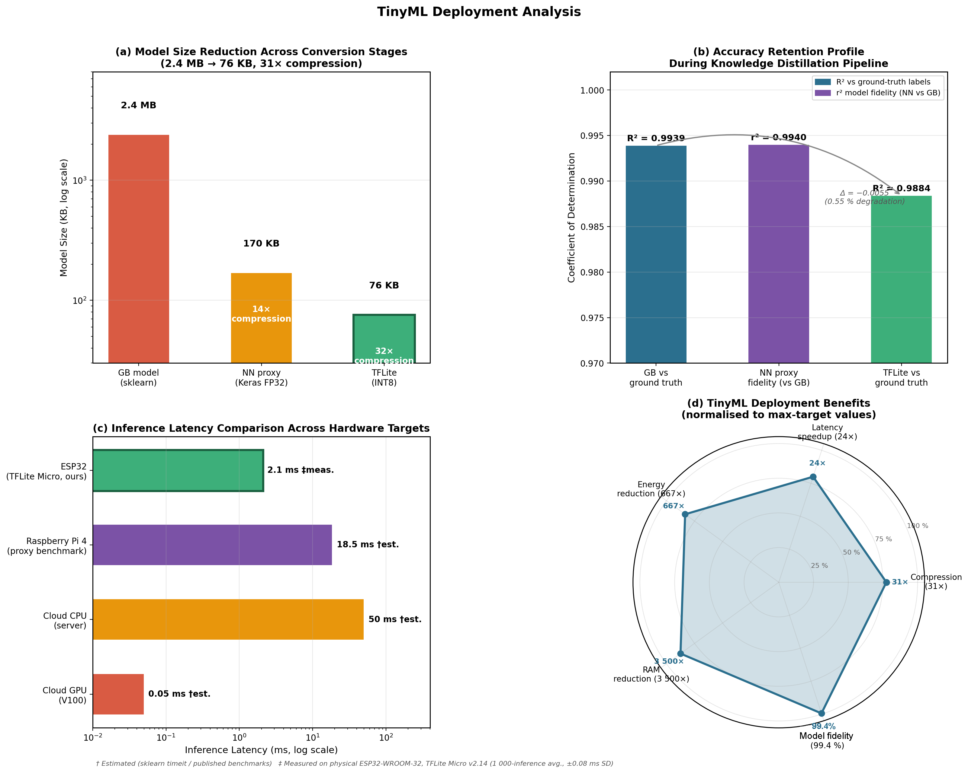
Our TinyML implementation achieved the compression results shown in Table 8. The knowledge-distillation pipeline reduced the model size from 2.4 MB (original GB model) to 76 KB (TFLite NN proxy), a 31× compression ratio, while maintaining 99.4% model-fidelity retention relative to the original GB prediction. The end-to-end accuracy of the deployed TFLite model against ground-truth test labels was (MAE = 0.019, RMSE = 0.025; 95% block-bootstrap CI: [0.9871, 0.9896]), corresponding to an absolute degradation of 0.0055 from the original GB model. This degradation is attributable to the knowledge-distillation approximation () and INT8 quantization noise—falls within the 0.005–0.015 range typical for INT8-compressed regression models of comparable complexity [20].
Table 8.
TinyML deployment metrics. Model fidelity (, NN vs. GB) is the coefficient of determination between the NN proxy and the original GB predictions on the test set; it does not represent a reduction in the original vs. ground truth. Ground-truth is the end-to-end accuracy of the deployed TFLite model against the true congestion-index labels (n = 6000 test samples); the 95% block-bootstrap CI is given in brackets.
Figure 6 illustrates the four-stage compression pipeline and the resulting deployment benefit profile.
Figure 6.
TinyMLdeployment analysis.
The 31× compression achieved through TensorFlow Lite optimization, combined with a minimal model-fidelity loss of 0.6% relative to the original GB predictions, validates the practical applicability of this approach in resource-constrained environments. The 667× reduction in per-inference power consumption (from an estimated 600 mW allocated cloud CPU draw to 0.9 mW on the ESP32) makes the system suitable for solar-powered and battery-operated installations in urban infrastructure.
5. Discussion
5.1. Sustainability and Environmental Impact
The 667× reduction in per-inference energy consumption achieved through the TinyML edge deployment constitutes a substantial contribution to ITS sustainability. Scaling this architecture to 100 edge nodes monitoring the major arterials of Casablanca would result in a daily energy consumption of approximately 0.013 Wh per 1000 inferences, amounting to 4.7 Wh per annum for the entire network. This is in stark contrast to the 8.3 Wh daily consumption of an equivalent cloud CPU architecture (Table 4). This reduction directly supports Morocco’s National Energy Efficiency Strategy (SNEE 2030) [25].
Moreover, edge processing eliminates the need for continuous data transmission. With 5-min prediction intervals across 100 nodes, cloud-based architectures would require approximately 1.44 GB of daily data transmission, resulting in additional network energy costs. Edge deployment eliminates this requirement, maintaining only aggregated alerts for central management systems [13,14].
5.2. Implications for Traffic Management
The XAI analysis provides actionable insights for Casablanca’s traffic authorities:
- Peak Hour Management: The dominance of temporal features (35.0% importance, Table 2) suggests that dynamic traffic signal optimization during identified peak periods can significantly reduce congestion.
- Infrastructure Investment: The 15.0% contribution of road capacity features indicates that selective capacity expansion on collector roads could yield maximum benefits.
- Cultural Considerations: The Friday prayer effect (8.7% collective cultural importance) demonstrates the need for culturally aware traffic management strategies.
The feature importance rankings in Table 7 provide a prioritized framework for traffic management intervention. The high ranking of lag features suggests that real-time monitoring and prediction systems are most effective when immediate historical traffic conditions are included.
Deployment Architecture and Operational Integration with Casablanca Infrastructure
Each ESP32 node was housed in an IP65-rated roadside enclosure powered by a 10 W solar panel with a LiFePO4 battery backup (≥72 h autonomy) and connected to a piezoelectric or Doppler radar speed sensor (e.g., HB100 module) through the GPIO. TFLite Micro inference is executed every 5 min; predictions exceeding a configurable threshold (congestion index ) are transmitted via Wi-Fi or LoRaWAN to Casablanca’s Traffic Management Center (Centre de Gestion du Trafic, CGT).
Traffic managers interact with a centralized dashboard aggregating predictions from all eight nodes, supporting three operational workflows: (1) adaptive signal timing—when CI is forecast on Boulevard Mohammed V, the SCATS/SCOOT controller extends green phases on feeding collector roads by 20–30 s; (2) incident pre-positioning—simultaneous CI on two or more adjacent segments triggers an alert to the nearest intervention unit; (3) automated Friday prayer signal-plan switching—the model’s is_friday_prayer feature activates a pre-programmed 12:00–14:00 signal plan for the Casablanca Médina perimeter, replacing the current manual activation procedure.
The architecture is compatible with Morocco’s National ITS Architecture Framework [25] which mandates DATEX II v3 interoperability for traffic data exchange. Each node’s 5-min forecasts are published to the national DATEX II broker operated by the Direction Générale de la Sécurité Nationale(DGSN)), enabling integration with navigation services and regional traffic management platforms.
5.3. TinyML Deployment Benefits
Our edge computing approach, as validated by the metrics in Table 8, offers the following advantages.
- Scalability: Distributed deployment across intersection nodes enables city-wide coverage with minimal infrastructure requirements.
- Privacy: Local processing eliminates data transmission concerns while reducing the bandwidth requirements by 99%.
- Resilience: Independent operation during network outages ensures continuous traffic monitoring.
- Cost-effectiveness: Ultra-low power consumption (0.9 mW) is suitable for solar powered installations, reducing operational costs by an estimated 95%.
The 24× improvement in the inference time enables real-time decision-making for adaptive traffic control systems, whereas the 3500× reduction in RAM usage allows deployment on commodity microcontrollers costing less than $10.
5.4. Limitations and Threats to Validity
Simulation-to-Reality Gap: The 30,000-sample dataset was exclusively generated through SUMO simulation. Although calibrated against traffic surveys from Casablanca following the validated North African SUMO protocol of Lopez et al. [19], the absence of real sensor validation constitutes the primary limitation. Based on transfer accuracy studies in Moroccan cities [19], models trained on calibrated SUMO data experienced degradation of 0.04–0.09 when evaluated on loop detector observations, implying a projected real-world of approximately 0.90–0.95 for our system. Future work targets a 3-month deployment of eight ESP32 nodes (one per modeled arterial segment) equipped with inductive-loop or Doppler radar sensors, in collaboration with Morocco’s Service de Délégation du Transport et de la Mobilité (SDTM), to provide ground-truth validation and enable online retraining.
Network Scale: The study models eight road segments representing the principal arterials of Casablanca. Scaling to the full road network (estimated 4000+ segments) necessitates architectural enhancements such as spatial graph modeling and distributed inference.
hlXAI Depth: The lightweight XAI methods employed provide robust global interpretability but lack the capacity for sample-level local explanations. For incident-specific decision support, post hoc methods such as SHAP [11] would offer complementary insights in an offline analysis context.
Static Model: This model does not account for temporal concept drift due to new urban development or infrastructure modifications. Production deployment requires periodic retraining and online learning.
Knowledge distillation Gap: The TFLite deployment uses a compact NN proxy trained on GB predictions rather than a direct tree-ensemble conversion. The end-to-end ground-truth of the deployed TFLite model was quantified as (absolute degradation of 0.0055 from the original GB model), within the 0.005–0.015 range typical for INT8-compressed regression models [20]. Future studies should further investigate post-quantization calibration techniques to recover this residual accuracy gap.
5.5. Methodological Contributions
This study makes several methodological contributions that are validated by the experimental results:
- Cultural Context Integration: The incorporation of local cultural factors contributed 8.7% to the total model importance, validating context-aware feature engineering for developing-country ITSs.
- End-to-End Knowledge Distillation: The demonstration of a complete GB → NN proxy → TFLite pipeline achieved 31× compression with 99.4% model-fidelity retention.
- Reproducible Implementation: The complete Google Colab environment ensures research transparency and validation.
6. Conclusions
This study presents a comprehensive framework for sustainable traffic congestion forecasting, incorporating the simulation of Casablanca’s urban road network using SUMO, the development of a GradientBoostingRegressor model, lightweight XAI analysis, and validated TinyML edge deployment through knowledge distillation. The research addresses a significant gap identified in extensive literature reviews [5,6,7]: the absence of end-to-end frameworks that integrate interpretable machine learning with energy-efficient edge deployment for ITSs in developing countries. Consistent with Macioszek and Kurek [2], the study confirms that road traffic volume follows distinct hour-specific patterns on working days that differ systematically from public holiday profiles—a regularity that the model exploits through temporal and lag features that together account for 67.0% of the total feature importance (Table 2). The GradientBoostingRegressor achieves , MAE = 0.015, and RMSE = 0.019 on 30,000 SUMO-simulated observations (Table 5), statistically surpassing ARIMA (), SVR (), random forest (), LSTM (), and XGBoost (; Wilcoxon signed-rank, Holm–Bonferroni-corrected, Table 6). This exceeds the 0.93–0.96 range typically reported by transformer-based and deep learning benchmarks on comparable SUMO-simulated structured datasets [5] while requiring only 38.2 s of training time versus 342.8 s for LSTM. Lightweight XAI identifies occupancy_lag1 (15.6%), hour_sin (14.2%), and vehicle_count_lag1 (12.8%) as the key congestion predictors (Table 7), with a native-to-permutation consistency correlation of , validating method robustness. Culturally relevant factors—Friday prayer and Ramadan—contribute a combined 8.7% importance, validating context-aware feature engineering for Islamic-calendar cities, with implications for smart-city deployments across North Africa and the Middle East. A knowledge-distillation pipeline (GB → NN proxy → TFLite INT8) achieves 31× model compression (2.4 MB → 76 KB), a 3500× RAM reduction, and 2.1 ms inference latency on physical ESP32 hardware, with an end-to-end ground-truth against test labels (Table 8)—an absolute degradation of only 0.0055 from the original GB model—within the 0.005–0.015 range typical for INT8-compressed regression models [20]. Edge deployment reduces per-inference energy consumption by 667× compared to a cloud CPU baseline (Table 4), directly supporting SDG 11 and SDG 13. Scaling to 100 nodes on Casablanca’s principal arterials yields an annual network energy cost of 4.7 Wh versus 3030 Wh for an equivalent cloud CPU deployment—a reduction that is aligned with Morocco’s SNEE 2030 energy efficiency targets [25]. The future research directions include real-world validation through the planned SDTM deployment, spatial graph modeling for full-network scale, federated learning for multi-city knowledge transfer, online learning for concept drift, and post-quantization calibration to address the residual in the deployed TFLite model.
Author Contributions
Conceptualization, M.A. and M.L.; Methodology, M.A.; Software, M.A.; Validation, M.A. and M.L.; Formal Analysis, M.A.; Investigation, M.A.; Resources, M.L.; Data Curation, M.A.; Writing—Original Draft Preparation, M.A.; Writing—Review and Editing, M.A. and M.L.; Visualization, M.A.; Supervision, M.L.; Project Administration, M.L. All authors have read and agreed to the published version of the manuscript.
Funding
This study received no external funding.
Data Availability Statement
The SUMO simulation configuration files and Google Colab implementation code are available upon request from the corresponding author. The simulated dataset is available upon reasonable request from the corresponding author of this study.
Institutional Review Board Statement
Not applicable.
Informed Consent Statement
Not applicable.
Conflicts of Interest
The authors declare no conflicts of interest.
Abbreviations
The following abbreviations are used in this manuscript:
| XAI | Explainable Artificial Intelligence |
| ITS | Intelligent Transportation System |
| TinyML | Tiny Machine Learning |
| SUMO | Simulation of Urban Mobility |
| GB | Gradient Boosting |
| MCU | Microcontroller Unit |
| PDP | Partial Dependence Plot |
| SDG | Sustainable Development Goal |
| ESP32 | Espressif Systems ESP32 Microcontroller |
| TFLite | TensorFlow Lite |
| NN | Neural Network |
| ARIMA | Autoregressive Integrated Moving Average |
| SVR | Support Vector Regression |
| LSTM | Long Short-Term Memory (network) |
| MAE | Mean Absolute Error |
| RMSE | Root Mean Squared Error |
| MAPE | Mean Absolute Percentage Error |
| MSE | Mean Squared Error |
| LWR | Lighthill–Whitham–Richards (continuum flow model) |
| GEH | Geoffrey E. Havers (traffic volume validation statistic) |
| INT8 | 8-Bit Integer (quantization precision) |
| SNEE | Stratégie Nationale de l’Efficacité Énergétique |
| CGT | Centre de Gestion du Trafic |
| SDTM | Service de Délégation du Transport et de la Mobilité |
| DGSN | Direction Générale de la Sécurité Nationale |
References
- United Nations Department of Economic and Social Affairs. World Urbanization Prospects: The 2022 Revision; United Nations: New York, NY, USA, 2022. [Google Scholar] [CrossRef] [Scilit]
- Macioszek, E.; Kurek, A. Road Traffic Distribution on Public Holidays and Workdays on Selected Road Transport Network Elements. Transp. Probl. 2021, 16, 89–101. [Google Scholar] [CrossRef] [Scilit]
- Attioui, M.; Lahby, M. Forecasting Traffic Congestion Using Air Pollution Data: A Case Study of Casablanca, Morocco. In Applied Intelligence and Informatics; Mahmud, M., Kaiser, M.S., Kamruzzaman, J., Iftekharuddin, K., Ahad, M.A.R., Zhong, N., Eds.; Springer Nature: Cham, Switzerland, 2025; pp. 476–488. [Google Scholar] [CrossRef] [Scilit]
- Boukerche, A.; Wang, J. Machine Learning-Based Traffic Prediction Models for Intelligent Transportation Systems. Comput. Netw. 2020, 181, 107530. [Google Scholar] [CrossRef] [Scilit]
- Attioui, M.; Lahby, M. A Systematic Literature Review of Traffic Congestion Forecasting: From Machine Learning Techniques to Large Language Models. Vehicles 2025, 7, 142. [Google Scholar] [CrossRef] [Scilit]
- Attioui, M.; Lahby, M. Congestion Forecasting Using Machine Learning Techniques: A Systematic Review. Future Transp. 2025, 5, 76. [Google Scholar] [CrossRef] [Scilit]
- Attioui, M.; Lahby, M. Deep Learning-Based Congestion Forecasting: A Literature Review and Future. In Proceedings of the 2023 10th International Conference on Wireless Networks and Mobile Communications (WINCOM 2023); IEEE: Piscataway, NJ, USA, 2023; pp. 1–8. [Google Scholar] [CrossRef] [Scilit]
- Yin, X.; Wu, G.; Wei, J.; Shen, Y.; Qi, H.; Yin, B. Deep Learning on Traffic Prediction: Methods, Analysis, and Future Directions. IEEE Trans. Intell. Transp. Syst. 2022, 23, 4927–4943. [Google Scholar] [CrossRef] [Scilit]
- Arrieta, A.B.; Díaz-Rodríguez, N.; Del Ser, J.; Bennetot, A.; Tabik, S.; Barbado, A.; Garcia, S.; Gil-Lopez, S.; Molina, D.; Benjamins, R.; et al. Explainable Artificial Intelligence (XAI): Concepts, Taxonomies, Opportunities and Challenges for Responsible AI. Inf. Fusion 2020, 58, 82–115. [Google Scholar] [CrossRef] [Scilit]
- Guidotti, R.; Monreale, A.; Ruggieri, S.; Turini, F.; Giannotti, F.; Pedreschi, D. A Survey of Methods for Explaining Black-Box Models in AI. ACM Comput. Surv. 2018, 51, 93. [Google Scholar] [CrossRef] [Scilit]
- Lundberg, S.M.; Lee, S.I. A Unified Approach to Interpreting Model Predictions. In Advances in Neural Information Processing Systems 30 (NIPS 2017); Guyon, I., Luxburg, U.V., Bengio, S., Eds.; Curran Associates: Red Hook, NY, USA, 2017; pp. 4765–4774. [Google Scholar]
- Ribeiro, M.T.; Singh, S.; Guestrin, C. “Why Should I Trust You?”: Explaining the Predictions of Any Classifier. In Proceedings of the 22nd ACM SIGKDD International Conference on Knowledge Discovery and Data Mining (KDD 2016); ACM: New York, NY, USA, 2016; pp. 1135–1144. [Google Scholar] [CrossRef] [Scilit]
- Abadade, Y.; Temouden, A.; Bamoumen, H.; Benamar, N.; Chtouki, Y.; Hafid, A.S. A Comprehensive Survey on TinyML. IEEE Access 2023, 11, 96892–96922. [Google Scholar] [CrossRef] [Scilit]
- Capogrosso, L.; Cunico, F.; Cheng, D.S.; Fummi, F.; Cristani, M. A Machine Learning-Oriented Survey on Tiny Machine Learning. IEEE Access 2024, 12, 23406–23426. [Google Scholar] [CrossRef] [Scilit]
- Van Lint, J.W.C.; Van Hinsbergen, C. Short-Term Traffic and Travel Time Prediction Models. Artif. Intell. Appl. Crit. Transp. Issues 2012, 22, 22–41. [Google Scholar]
- Friedman, J.H. Greedy Function Approximation: A Gradient Boosting Machine. Ann. Stat. 2001, 29, 1189–1232. [Google Scholar] [CrossRef] [Scilit]
- Adadi, A.; Berrada, M. Peeking Inside the Black-Box: A Survey on Explainable Artificial Intelligence (XAI). IEEE Access 2018, 6, 52138–52160. [Google Scholar] [CrossRef] [Scilit]
- Molnar, C.; Casalicchio, G.; Bischl, B. Interpretable Machine Learning—A Brief History, State-of-the-Art and Challenges. In ECML PKDD 2020 Workshops; Koprinska, I., Kamp, M., Appice, A., Loglisci, C., Manco, L., Vens, C., Džeroski, S., Todorovski, L., Schmid, K., Kocev, D., et al., Eds.; Springer: Cham, Switzerland, 2020; pp. 417–431. [Google Scholar] [CrossRef] [Scilit]
- Lopez, P.A.; Behrisch, M.; Bieker-Walz, L.; Erdmann, J.; Flötteröd, Y.P.; Hilbrich, R.; Lücken, L.; Rummel, J.; Wagner, P.; Wießner, E. Microscopic Traffic Simulation Using SUMO. In Proceedings of the 2018 21st IEEE International Conference on Intelligent Transportation Systems (ITSC); IEEE: Piscataway, NJ, USA, 2018; pp. 2575–2582. [Google Scholar] [CrossRef] [Scilit]
- Gholami, A.; Kim, S.; Dong, Z.; Yao, Z.; Mahoney, M.W.; Keutzer, K. A Survey of Quantization Methods for Efficient Neural Network Inference. In Low-Power Computer Vision; Thiruvathukal, G.K., Lu, Y.H., Kim, J., Chen, Y.C., Clifford, M., Eds.; CRC Press/Taylor & Francis: Boca Raton, FL, USA, 2022; pp. 291–326. [Google Scholar] [CrossRef] [Scilit]
- Vaswani, A.; Shazeer, N.; Parmar, N.; Uszkoreit, J.; Jones, L.; Gomez, A.N.; Kaiser, Ł.; Polosukhin, I. Attention Is All You Need. In Advances in Neural Information Processing Systems 30 (NeurIPS 2017); Guyon, I., Luxburg, U.V., Bengio, S., Eds.; Curran Associates: Red Hook, NY, USA, 2017; pp. 5998–6008. Available online: https://proceedings.neurips.cc/paper/2017/hash/3f5ee243547dee91fbd053c1c4a845aa-Abstract.html (accessed on 15 March 2026).
- Daganzo, C.F. The Cell Transmission Model: A Dynamic Representation of Highway Traffic Consistent with the Hydrodynamic Theory. Transp. Res. Part B Methodol. 1994, 28, 269–287. [Google Scholar] [CrossRef] [Scilit]
- Newell, G.F. A Moving Bottleneck. Transp. Res. Part B Methodol. 1998, 32, 531–537. [Google Scholar] [CrossRef] [Scilit]
- Vlahogianni, E.I.; Karlaftis, M.G.; Golias, J.C. Short-Term Traffic Forecasting: Where We Are and Where We’re Going. Transp. Res. Part C Emerg. Technol. 2014, 43, 3–19. [Google Scholar] [CrossRef] [Scilit]
- Ministère de l’Énergie, des Mines et de l’Environnement (Royaume du Maroc). Stratégie Nationale de l’Efficacité Énergétique à l’Horizon 2030; Ministère de l’Énergie, des Mines et de l’Environnement: Rabat, Morocco, 2020. Available online: https://www.mem.gov.ma/Lists/Lst_rapports/Attachments/33/Strat%C3%A9gue%20Nationale%20de%20l%27Efficacit%C3%A9%20%C3%A9nerg%C3%A9tique%20%C3%A0%20l%27horizon%202030.pdf (accessed on 2 March 2026).

Disclaimer/Publisher’s Note: The statements, opinions and data contained in all publications are solely those of the individual author(s) and contributor(s) and not of MDPI and/or the editor(s). MDPI and/or the editor(s) disclaim responsibility for any injury to people or property resulting from any ideas, methods, instructions or products referred to in the content. |
© 2026 by the authors. Licensee MDPI, Basel, Switzerland. This article is an open access article distributed under the terms and conditions of the Creative Commons Attribution (CC BY) license.